Inverse Potentials for $\alpha-\alpha$ Scattering using Gaussian Interaction

Abstract

Alpha-alpha scattering phase shifts (SPS) have been determined using phase function method (PFM) with local nuclear interaction between two alpha clusters modeled as double Gaussian potential and Coulomb repulsion in the form of $erf()$ function. The obtained SPS for various $\ell$-channels have been compared with experimental ones with mean absolute percentage error (MAPE) as a measure. The model parameters have been optimised by suitable optimisation technique by looking for minimum value of MAPE. The results for $\ell$=0⁺, 2⁺ and 4⁺ partial waves have been obtained, to match with experimental SPS, with MAPE values of $7.6$, $2.7$ and $6.5$ respectively for data up to $120$ MeV, while for higher states 6⁺, 8⁺ and 10⁺ has MAPE of $1.7,7.4$ and $10.4$ respectively for data from $53-120$ MeV. On extrapolation for data in range E_ℓab. = $23-120$ MeV, using the optimised parameters, the SPS are found to be in close agreement with experimental ones for first three channels.

keywords: alpha-alpha scattering, phase function method (PFM), scattering phase shifts, Double Gaussian potential

1 Introduction

To understand the structure of nucleus one of the essential methods involved is scattering phenomena. The core purpose of this paper is to investigate scattering of alpha particles which are in relative motion for all partial waves. Rutherford and Chadwick were the first who experimentally studied $\alpha-\alpha$ scattering in the year 1927 and since then a large amount of experimental data is available given by (i) Afzal et al. [1] (ii) S. Chien and Ronald E brown [2] (iii) Igo [3] (iv) Darriulat, Igo,Pug, Holm [4](v) Nilson [5] and others. Alpha-alpha problem has been extensively studied both experimentally and theoretically with alpha particle having some sole properties like (i) zero spin and isospin (ii) tight binding energy of $28.3$ MeV having property to form cluster like states for lighter nuclei (^6,7Li, ⁹Be, ¹²C and ¹⁶O are $\alpha$-structured) with alpha particle being the core nuclei in the cluster (iii) small root mean square radius of $1.44$ fm.
In 1940’s for $\alpha-\alpha$ scattering experiments only naturally occurring $\alpha$-sources like polonium, thorium and radium were used, which did not result in very accurate results from experiments. Later on, with the advancement of technology, accelerators were used in scattering processes and highly accurate phase shifts were observed. The importance of $\alpha-\alpha$ scattering is that the study provides information regarding force field in nearest surrounding of He-nuclei and also provide information regarding energy levels of ⁸Be nucleus.
Haéfner was one of the first who studied ⁸Be properties in 1951 by using phenomenological potential [6]. Later on Nilson, Briggs, Jentschke and others used Haéfner potential for $\ell=$2 state from the ground state of $96$ KeV. Later on, Nilson et al. [5] extended Hafner model [6] to include $\ell$= 0, 2 and 4 and found that best agreement of phase shift with experiments require small value of $R=3.49$ fm. Also, Nilson found that testing the efficiency of the potential required data above $22.9$ MeV, which was unfortunately not available at that time. Later in the year 1958 Spuy and Pienaar [7] made phenomenological analysis up to $6$ MeV where they concluded that for $E<6$ MeV one needed velocity dependent interaction for fitting S and D waves. Later on, Wittern [8] in the year 1959 derived same semi-phenomenological potential and reached to same conclusion as given by Spuy and Pienaar. Later from 1960-1965 more phenomenological study was done by Igo who made optical model analysis for $\alpha-\alpha$ in range $E=23.1-47.1$ MeV and Darriulat, Igo and Pugh [3] who used energy independent but strongly $\ell$ dependent complex Wood Saxon potential for range $E=53-120$ MeV where they failed to fit the phase shifts using one single common potential for all the partial waves. Thus, it has been concluded, that single potential common to all $\ell$ do not exist phenomenologically. In short, $\alpha-\alpha$ potentials are found to be strongly $\ell$ dependent.
Buck et al. [9] used Gaussian potential of the form

$$V(r)=-V_{a}exp{(-\alpha r^{2})}+z_{1}z_{2}\frac{e^{2}}{r}erf(\beta r)$$ (1)

having single term with only two free parameters V_a ($-122.6225$ MeV) and $\alpha$ ($0.22$ $fm^{-2}$). The erf() function was included to take into account for the Coulomb interaction and model parameters were obtained to fit all even $\ell$ channels upto $E_{\ell ab.}<$ $80$ MeV. Ali and Bodmer [10] proposed two term phenomenological potential with 4 parameters and was able to fit the phase shift for $\ell$ = 0, 2 and 4 partial waves with good accuracy to the experimental data. Later Darriulat et al., [4] used the following Woods-Saxon potential, which has more than 6 parameters:

$$V_{\alpha\alpha}(r)=\frac{U_{1}}{[1+exp(r-r_{1})/a_{1}]}-\frac{U_{2}}{[1+exp(r-r_{2})/a_{2}]}+i\frac{W}{[1+exp(r-r_{3})/a_{3}]}+V_{C}(r)$$ (2)

with inelastic effects duly included in it for laboratory energy $53-120$ MeV and $\ell$= 0, 2, 4, 6, 8 and 10 partial waves phase shift was fitted for $E>53$ MeV.
Phase function method (PFM) was used by Jana et al. [11] for $\alpha-\alpha$ scattering by using angular momentum-dependent complex Saxon-Woods potential as was suggested by Darriulat et al for $\ell$=0,2 and 4 partial wave only. Odsuren et al. [12] calculated partial scattering cross section using Gaussian potential for $\alpha-\alpha$, $n-\alpha$ and $p-\alpha$ using complex scaling method (CSM). Scattering phase-shifts are commonly obtained analytically using S-matrix [13] and Jost function methods [14]. Recently, there has been a renewed interest in the use of Phase function method (PFM) or Variable phase approach (VPA) by Laha and group and they have applied the method for studying various light nuclei scattering problems which include study of nucleon-nucleon (N-N), nucleon-nucleus (N-n) and nucleus-nucleus (n-n) [15, 16, 17, 18] scattering using a variety of two term potentials such as modified Hulthen and Manning-Rosen. While traditional S-matrix approaches depend on wave-functions obtained by solving time independent Schr$\ddot{o}$dinger equation (TISE), PFM requires only potential function to obtain the scattering phase shifts.
In this paper, our main objective is to obtain the scattering phase-shifts for alpha-alpha system using two term Gaussian potential and Coulomb term included as an $erf()$ function in elastic region only i.e ($E_{\ell}$=$0-23$ MeV) by employing PFM for all even partial waves including $\ell$ = 6, 8 and 10. We have included above partial waves because although their contribution to total cross section is small, but it can not be neglected. Above elastic region we have extrapolated the results upto $120$ MeV energies. Instead of following Ali procedure [10] we have given free run to the parameters for all partial waves. We have extended the calculations for higher $\ell$ channels like $\ell$=6,8 and 10 which is missing in Ali et al. work. PFM has been employed in tandem with model parameter optimising technique to obtain the results.

2 Methodology:

2.1 Model of Interaction:

The interaction between the two alpha particles is written as a combination of nuclear and Coulomb part as

$$V_{\alpha\alpha}=V_{\alpha\alpha}^{(N)}+V_{C}$$ (3)

where the nuclear part is

$$V_{\alpha\alpha}^{(N)}(r)=V_{r}exp(-\mu_{r}^{2}r^{2})-V_{a}exp(-\mu_{a}^{2}r^{2})$$ (4)

Here, V_r is attraction strength and V_a is repulsion in MeV. $\mu_{r}$ and $\mu_{a}$ are the inverse ranges in $fm^{-2}$. The Coulomb potential $V_{c}$ is having form

$$V_{c}=\frac{4e^{2}}{r}erf(\beta r)~{}~{}\text{and}~{}~{}\beta=\frac{\sqrt{3}}{2R_{\alpha}}$$ (5)

Interaction from this expression is called as improved Coulomb interaction. It is due to finite size of the $\alpha$-particles, which is given by RMS value of its radius. That is, R_α = 1.44 fm.

2.2 Phase Function Method:

The Schr$\ddot{o}$dinger wave equation for a spinless particle with energy E and orbital angular momentum $\ell$ undergoing scattering with interaction potential V(r) is given by

$$\frac{\hbar^{2}}{2\mu}\bigg{[}\frac{d^{2}}{dr^{2}}+\bigg{(}k^{2}-\frac{\ell(\ell+1)}{r^{2}}\bigg{)}\bigg{]}u_{\ell}(k,r)=V(r)u_{\ell}(k,r)$$ (6)

Where

$$k_{c.m}=\sqrt{\frac{2\mu E_{c.m}}{{\hbar^{2}}}}~{}fm^{-1}$$ (7)

with $\frac{\hbar^{2}}{2\mu}=10.44217$ MeV $fm^{2}$. For $\alpha-\alpha$ system, centre of mass energy $E_{c.m.}$ is related to laboratory energy by following relation for non-relativistic kinematics

$$E_{c.m}=\frac{M_{\alpha}}{M_{\alpha}+M_{\alpha}}E_{\ell ab}=0.5E_{\ell ab}$$ (8)

PFM or VPA is one of the important tools in scattering studies for both local [19] and non-local interactions [11]. The mathematical foundation of PFM method is well known in theory of differential equations, that a linear homogeneous equation of second order, such as Schr$\ddot{o}$dinger equation , can be reduced to a nonlinear differential equation (NDE) of first order-the Riccati equation [20]. The phase equation which was independently worked out by Calogero [21] and Babikov [22] is written in the following form.

$$\delta_{\ell}^{\prime}(k,r)=-\frac{V(r)}{k(\hbar^{2}/2\mu)}\big{[}\cos(\delta_{\ell}(r))\hat{j}_{\ell}(kr)-\sin(\delta_{\ell}(r))\hat{\eta}_{\ell}(kr)\big{]}^{2}$$ (9)

This NDE is numerically integrated from origin to the asymptotic region using suitable numerical techniques, thereby obtaining directly the values of scattering phase shift for different values of projectile energy in laboratory frame. The central idea of VPA is to obtain the phase shift $\delta$ directly from physical quantities such as interaction potential V(r), instead of solving TISE for wave functions u(r), which in turn are used to determine $\delta_{\ell}(k,r)$. With initial condition $\delta(0)=0$. The phase shift $\delta_{\ell}$ can be seen as real function of $k$ and characterizes the strength of scattering of any partial wave i.e. say $\ell^{th}$ partial wave of the potential V(r). In the above equation and are the Bessel functions. Since we are only focusing on obtaining scattering phase shifts for $\ell$= 0 partial wave, the Riccati-Bessel function [21] is given by $\hat{j_{0}}=\sin(kr)$ and similarly the Riccati-Neumann function is given by $\hat{\eta_{0}}=-\cos(kr)$, thus reducing eq. 9 to

$$\delta_{0}^{\prime}(k,r) =\begin{aligned} &-\frac{V(r)}{k(\hbar^{2}/2\mu)}\bigg{[}\sin(kr+\delta_{0})\bigg{]}^{2}\\ \end{aligned}$$ (10)

PFM equation for D-wave takes following form

$$\delta_{2}^{\prime}(k,r) =\begin{aligned} &-\frac{V(r)}{k(\hbar^{2}/2\mu)}\bigg{[}-\sin{\left(kr+\delta_{2}\right)}-\frac{3\cos{\left(\delta_{2}+kr\right)}}{kr}+\frac{3\sin{\left(\delta_{2}+kr\right)}}{k^{2}r^{2}}\bigg{]}^{2}\\ &\end{aligned}$$ (11)

PFM equation for G-wave takes following form

$$\delta_{4}^{\prime}(k,r) =\begin{aligned} \begin{cases}&-\frac{V(r)}{k(\hbar^{2}/2\mu)}\bigg{[}\sin{\left(\delta_{4}+kr\right)}+\frac{10\cos{\left(\delta_{4}+kr\right)}}{kr}-\frac{45\sin{\left(\delta_{4}+kr\right)}}{k^{2}r^{2}}-\frac{105\cos{\left(\delta_{4}+kr\right)}}{k^{3}r^{3}}\\ &+\frac{105\sin{\left(\delta_{4}+kr\right)}}{k^{4}r^{4}}\bigg{]}^{2}\end{cases}\end{aligned}$$ (12)

PFM equation for $$\ell$$=6 is

$$\delta_{6}^{\prime}(k,r) =\begin{aligned} &-\frac{V(r)}{k(\hbar^{2}/2\mu)}\bigg{[}\cos(\delta_{6}(k,r))\hat{\tau}(kr)-\sin(\delta_{6}(r))\hat{\xi}(kr)\bigg{]}^{2}\end{aligned}$$ (13)

where $$\hat{\tau}(kr)$$ is calculated as

$$\hat{\tau}(kr) =\begin{aligned} \begin{cases}&(kr)^{6}\bigg{\{}\bigg{(}-21(kr)\bigg{[}495-60(kr)^{2}+(kr)^{4}\bigg{]}\cos(kr)\\ &+\bigg{[}-10395+4725(kr)^{2}-210(kr)^{4}+(kr)^{6}\bigg{]}\sin(kr)\bigg{)}\bigg{\}}\end{cases}\end{aligned}$$ (14)

and $$\hat{\xi}(kr)$$ is calculated as

$$\hat{\xi}(kr) =\begin{aligned} \begin{cases}&(kr)^{6}\bigg{\{}\bigg{(}-21(kr)\bigg{[}495-60(kr)^{2}+(kr)^{4}\bigg{]}\sin(kr)\\ &+\bigg{[}-10395+4725(kr)^{2}-210(kr)^{4}+(kr)^{6}\bigg{]}\cos(kr)\bigg{)}\bigg{\}}\end{cases}\end{aligned}$$ (15)

PFM equation for $$\ell$$=8 is

$$\delta_{8}^{\prime}(k,r) =\begin{aligned} &-\frac{V(r)}{k(\hbar^{2}/2\mu)}\bigg{[}\cos(\delta_{8}(k,r))\hat{\zeta}(kr)-\sin(\delta_{8}(k,r))\hat{\chi}(kr)\bigg{]}^{2}\end{aligned}$$ (16)

where we have

$$\hat{\zeta}(kr) =\begin{aligned} \begin{cases}&\frac{1}{(kr)^{8}}\bigg{\{}9(kr)\bigg{[}-225225+30030(kr)^{2}-770(kr)^{4}+4(kr)^{6}\bigg{]}\cos(kr)\\ &+\bigg{[}2027025-945945(kr)^{2}+51975(kr)^{4}-630(kr)^{6}+(kr)^{8}\bigg{]}\sin(kr)\bigg{\}}\end{cases}\end{aligned}$$ (17)

and $$\hat{\chi}(kr)$$ is calculated to be

$$\hat{\chi}(kr) =\begin{aligned} \begin{cases}&\frac{1}{(kr)^{8}}\bigg{\{}9(kr)\bigg{[}-225225+30030(kr)^{2}-770(kr)^{4}+4(kr)^{6}\bigg{]}\sin(kr)\\ &-\bigg{[}2027025-945945(kr)^{2}+51975(kr)^{4}-630(kr)^{6}+(kr)^{8}\bigg{]}\cos(kr)\bigg{\}}\end{cases}\end{aligned}$$ (18)

PFM equation for $$\ell$$=10 takes form

$$\delta_{10}^{\prime}(k,r) =\begin{aligned} &-\frac{V(r)}{k(\hbar^{2}/2\mu)}\bigg{[}\cos(\delta_{10}(k,r))\hat{\kappa}(kr)-\sin(\delta_{10}(k,r))\hat{\gamma}(kr)\bigg{]}^{2}\end{aligned}$$ (19)

where $$\hat{\kappa}(kr)$$ is calculated to be

$$\hat{\kappa}(kr) =\begin{aligned} \begin{cases}&-(55(kr)\bigg{[}11904165-1670760(kr)^{2}+51597(kr)^{4}-4684(kr)^{6}\\ &+(kr)^{8}\bigg{]}\cos(kr)+\bigg{[}-654729075+310134825(kr)^{2}-18918900(kr)^{4}\\ &+315315(kr)^{6}-1485(kr)^{8}+(kr)^{10}\bigg{]}\sin(kr))(kr)^{-10}\end{cases}\end{aligned}$$ (20)

and $$\hat{\gamma}(kr)$$ comes out to be

$$\hat{\gamma}(kr) =\begin{aligned} \begin{cases}&-(55(kr)\bigg{[}11904165-1670760(kr)^{2}+51597(kr)^{4}-4684(kr)^{6}\\ &+(kr)^{8}\bigg{]}\sin(kr)+\bigg{[}-654729075+310134825(kr)^{2}-18918900(kr)^{4}\\ &+315315(kr)^{6}-1485(kr)^{8}+(kr)^{10}\bigg{]}\cos(kr))(kr)^{-10}\end{cases}\end{aligned}$$ (21)

These NDE’s equations (10-19) are numerically integrated from origin to the asymptotic region using RK-4/5 method, thereby obtaining directly the values of scattering phase shift for different values of projectile energy in lab frame. The central idea of VPA is to obtain the phase shift $\delta$ directly from physical quantities such as interaction potential V(r), instead of solving TISE for wave functions $u(r)$, which in turn are used to determine $\delta$.

3 Simulation of Results and Discussion

Here, we have used double Gaussian potential and calculated the SPS using phase function method (PFM). Our obtained potentials are real and are obtained at elastic energies, $E_{\ell ab.}$= 0-23 MeV. The extrapolated curves are just an indication of how phase shift varies at higher energies (E $>$ 23 MeV) and are observed to be in good match with the experimental data upto 120 MeV on extrapolation. Some distortion from the experimental data above 23 MeV may be due to the absence of inelastic potential in our calculations. We have extended our work by taking additional $\ell$ = 6, 8 and 10 partial wave data which have not been investigated using PFM in any recent literature.
Potentials associated with partial waves are shown in figures 3. Standard procedures were used to numerically calculate the phase shifts using equations (10-19). Our approach has been to vary all the 4 parameters for $\ell$ = 0-10, but we observed that for $\ell$ = 0, 2 and 4 all parameters are required to get their respective phase shifts but for $\ell$ = 6, 8 and 10, it was observed that keeping or removing the repulsive core did not effect the phase shifts i.e. MAPE almost remained same, this must be due to the centrifugal barrier concealing the inner repulsive core. So, only two parameters were adjusted by to get phase shifts for $\ell$ = 6, 8 and 10 partial waves. Similar observation was found in work done recently by Darriulat [4] and Laha et al. [15] where it was observed that a single static potential can not give phase shift for all the partial waves. Double term Gaussian potential is giving similar nature potential as was given by Darriulat et al. with repulsive core and an attractive outer region. At $E_{\ell ab.}$ = 0.6 MeV the value of our phase shift for $\ell$ = 0 is 182.2 degree while experimental value is 178 $\pm$ 1 degree. Phase shift for $\ell$ = 0 changes its sign at $E_{\ell ab.}$ = 20 MeV, which is in close agreement to the work done by Ali and Bodmer [10], Tombrello and Senhouse [23] and Afzal [1] and continues to be in negative phase up to highest beam energy used ($120$ MeV). Our S-wave phase shift are consistent with experimental data (with MAPE=0.86$\%$) above $23$ MeV even on extrapolation and can be clearly observed in figure 2. D-wave phase shift become appreciable at $E_{\alpha}$ $>2.5$ MeV and at $E_{\ell ab}$=11.8 MeV maximum value of our phase shift for $\ell$ = 2 is 115.56 degree while experimental value is 114.9$\pm$2 degree, while the G-wave shift rises from $E_{\alpha}$ $>11$ MeV and at $E_{\ell ab}$=77.5 MeV maximum value of our phase shift for G-wave is $140.52$ degree while experimental value is 137 $\pm$ 1.8 degree. The $\ell$=6 and $\ell$=8 phase shifts can be seen to become active above $E_{\alpha}$ $\approx$ $30$ and $50$ MeV respectively.
The repulsive core for $\ell$=0 is more strong than D, G, I, K and M partial waves which can be observed form figure 3 and thus our potential is consistent with the results of Darriulat and Laha et al. Here it should be noted that the attractive interaction between two alpha particles is an important element which is responsible for keeping the nuclei against Coulombic repulsion. Also here it should be noted that the potential for $\ell$=6,8 and 10 in figure 3 should not be taken too seriously since experimental data above $54$ MeV was only considered to get the nature of interaction so it must be dealt cautiously. By utilising PFM method we have been able to construct appropriate phenomenological potential for entire range of energy for $\ell$=0-10 partial waves without incorporating the effects of inelastic processes. Including inelastic process may further bring down the MAPE and may even give approximate realistic potentials for the entire energy range.

States	$V_{a}$ (MeV)	$\mu_{a}$ $(fm^{-2})$	$V_{r}$ (MeV)	$\mu_{r}$ $(fm^{-2})$	MAPE (%)
$S^{+}$	15.2767	0.1851	693.912	0.942	7.6
$D^{+}$	73.9102	0.4741	334.852	1.0441	2.7
$G^{+}$	246.917	0.47458	235.731	3.9989	6.5
$I^{+}$	184.747	0.63178	–	–	1.7
$K^{+}$	6.28974	0.2271	–	–	7.4
$M^{+}$	12.2422	0.25907	–	–	10.4

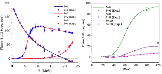
Figure 1: Phase shift for S,D,G (Left) and I,K, M (Right) states. Experimental data is taken from Heydenberg and Temmer, Russel, Phillips and Reich and Jones, Phillips and Miller E=0.15-9 MeV (1956-60), Nilson, Jentschke, Briggs, Kerman, Snyder E=12.3-22.9 MeV (1958).

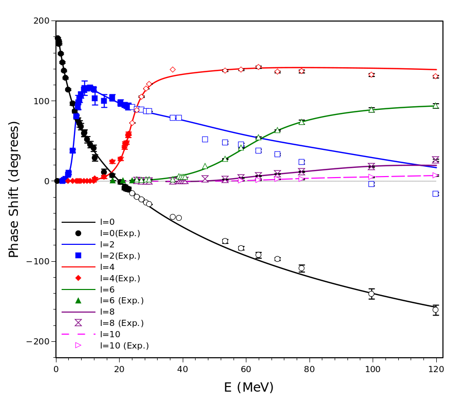
Figure 2: Phase shift for S,D,G,I,K and M-states. From 23 MeV on wards we have extrapolated data all the way up to 120 MeV only for first three channels. Experimental data is taken from Heydenberg and Temmer, Russel, Phillips and Reich and Jones, Phillips and Miller E=0.15-9 MeV (1956-60), Nilson, Jentschke, Briggs, Kerman, Snyder E=12.3-22.9 MeV (1958), Igo E=23.1-47.1 MeV (1960), Tombrello and Senhouse E=3.84-11.88 MeV (1963), Darriulat, Igo and Pugh E=53-120 MeV (1965) and Chen and Ronald E=18-29.5 MeV (1974).

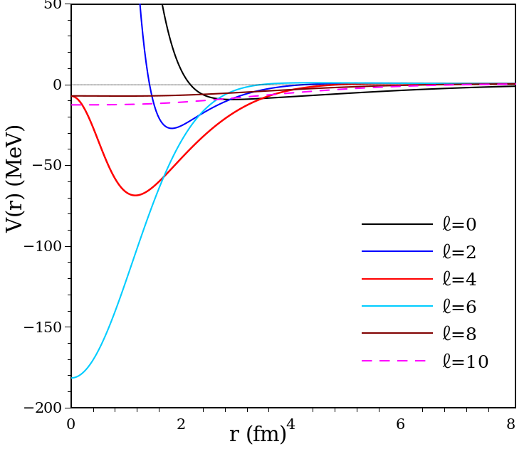
Figure 3: Potential plots for all channels without centrifugal potential a function of distance $r$(fm).

3.1 Phase shift, amplitude and wavefunction vs. distance $r$(fm)

One can use equations provided by Zhaba [25] to obtain scattering amplitudes and wavefunctions for various partial waves .The phase shift, amplitude and wavefunction plots for $\ell$=0, 2 and 4 states are shown in figure 4.

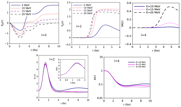
Figure 4: Phase shift vs. $r$ and amplitude vs. $r$ plots for $\ell$=0, 2 and 4 states.

Amplitude function equation for $$\ell=0$$ is given as

$$A_{0}^{\prime}= \begin{aligned} &-\frac{A_{0}V(r)}{k\left(\frac{\hbar^{2}}{2\mu}\right)}\left[\cos\delta_{0}\sin(kr)-\sin\delta_{0}(-\cos(kr))\right]\\ &\times\left[\sin\delta_{0}\sin(kr)+\cos\delta_{0}(-\cos(kr))\right]\end{aligned}$$ (23)

Amplitude function equation for $$\ell=2$$ is given as

$$A_{2}^{\prime}= \begin{aligned} &-\frac{A_{2}V(r)}{k\left(\frac{\hbar^{2}}{2\mu}\right)}\left[\cos\delta_{2}\left(\left(\frac{3}{(kr)^{2}}-1\right)\sin(kr)-\frac{3}{(kr)}\cos(kr)\right)\right.\\ &\times\left(\sin\delta_{2}\left(\left(\frac{3}{(kr)^{2}}-1\right)\sin(kr)-\frac{3}{(kr)}\cos(kr)\right)+\cos\delta_{2}\left(\left(-\frac{3}{(kr)^{2}}+1\right)\cos(kr)\right.\right.\\ &\left.\left.-\frac{3}{(kr)}\sin(kr)\right)\right]\end{aligned}$$ (24)

Similarly one can obtain amplitude equation for $$\ell=4$$ wave.

3.1.1 Wavefunction vs. distance $r$(fm)

The equation and figures for wavefunction vs. $r$(fm) for $\ell$=0, 2 and 4 states are given in figures 5.

Wavefunction equation for $$\ell=0$$ is given as

$$u_{0}(r)= \begin{aligned} A_{0}(r)\left[\cos\delta_{0}(r)\cdot\sin(kr)-\sin\delta_{0}(r)\cdot\cos(kr)\right]\\ \end{aligned}$$ (27)

Wavefunction equation for $$\ell=2$$ is given as

$$u_{2}(r)= \begin{aligned} &A_{2}(r)\left[\cos\delta_{2}(r)\left(\left(\frac{3}{(kr)^{2}}-1\right)\sin(kr)-\frac{3}{(kr)}\cos(kr)\right)\right.\\ &\left.-\sin\delta_{2}(r)\left(-\left(-\frac{3}{(kr)^{2}}+1\right)\cos(kr)-\frac{3}{(kr)}\sin(kr)\right)\right]\end{aligned}$$ (28)

Similarly one can obtain $$\ell=4$$ wavefuncton

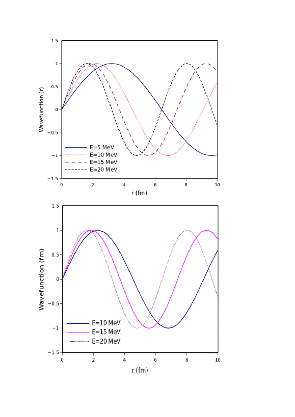
Figure 5: Wavefunction vs $r$(fm) plots for $\ell$=0, 2 and 4 states.

3.2 Cross-section:

Partial cross-section plot is shown in Fig. 2 for different states calculated using the obatained SPS values. Partial cross-section has been calculated by expression [24]

$$\sigma_{\ell}=\frac{4\pi}{k^{2}}(2\ell+1)\sin^{2}{\delta_{\ell}(k)}$$ (30)

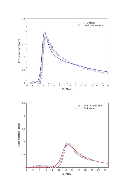
Figure 6: Cross section for D and G channels as function of center of mass energy $E_{C.M}$.

4 Conclusion

The scattering phase shifts for $\ell$ = 0 (S-channel), $\ell$ = 2 (D-channel) and $\ell$ = 4 (G-channel) have been computed upto 23 MeV and the best fitted parameters are found to give good match with the experimental data when extrapolated to the inelastic region of E $>$ 40 MeV up to $120$ MeV. For $\ell$ = 6 (I-channel), $\ell$ = 8 (K-channel) and $\ell$ = 10 (M-channel) also, a good match has be seen with the experimental data. Including inelastic process may further bring down the MAPE and may even give approximate realistic potentials for the entire energy range and shall be taken up in future. At last, the computed cross section results are compared with that of Odsuren et al., and are found to be in good agreement. In addition to earlier works done by Laha et al., using PFM for $\ell$ = 0, 2 and 4, we have explored the applicability of PFM to even higher states upto $\ell$ = 6, 8 and 10. Thus, PFM stands as an efficient tool for phase shift calculations in quantum mechanical scattering problems for local as well as non-local potentials. We may summarise our entire work in 3 main points:
(i) Double Gaussian potential results in effective inverse interaction potentials for alpha-alpha scattering for all $\ell$-channels.
(ii) Phase Function Method has been shown to be an effective tool for phase shift calculations.
(iii) Phases shifts calculated for elastic region have been found to give good results for inelastic energy data upto $120$ MeV for all partial waves.

References

- [1] Afzal S. A., Ahmad A. A. Z. and Ali S. (1969). Systematic Survey of the Interaction, Rev. Mod. Phys. 41, 247. https://doi.org/10.1103/RevModPhys.41.247
- [2] Chien W. S. and Brown R. E. (1974). Study of the system below 15 MeV (c.m.), Phys. Rev. C 10, 1767. https://doi.org/10.1103/PhysRevC.10.1767
- [3] Igo, G. (1960). Optical model analysis of the scattering of alpha particles from helium, Phys. Rev. 117, 1079. https://doi.org/10.1103/PhysRev.117.1079
- [4] Darriulat P., Igo G., Pugh H. G. and Holmgren H. D. (1965). Elastic Scattering of Alpha Particles by Helium Between 53 and 120 MeV, Phys. Rev. 137, B315 . https://doi.org/10.1103/PhysRev.137.B315
- [5] Nilson R., Jentschke W. K., Briggs G. R., Kerman R. O., and Snyder J. N. (1958). Investigation of Excited States in Be8 by Alpha-Particle Scattering from He, Phys. Rev. 109, 850. https://doi.org/10.1103/PhysRev.109.850
- [6] Haéfner, R. R. (1951). Rotational Energy Levels of an Alpha-Particle Model for the Beryllium and Carbon Isotopes, Rev. Mod. Phys. 23, 228. https://doi.org/10.1103/RevModPhys.23.228
- [7] Van-der Spuy, E. and Pienaar H.J. (1958). The interaction of two alpha-particles. Nucl. Phys. 7, 397-410. https://doi.org/10.1016/0029-5582(58)90278-5
- [8] Wittern, H., (1959). On the Interpretation of Scattering, Natural Sciences, 46, 443-444. https://doi.org/10.1007/BF00684320
- [9] Buck B., Friedrich H. and Wheatley C. (1977). Local potential models for the scattering of complex nuclei, Nucl. Phys. A 275, 246 . https://doi.org/10.1016/0375-9474(77)90287-1 Tombrello
- [10] Ali S. and Bodmer A. R. (1966). Phenomenological potentials, Nucl. Phys. 80, 99-112. https://doi.org/10.1016/0029-5582(66)90829-7
- [11] Jana A. K., Pal J., Nandi T. and Talukdar B. (1992). Phase-function method for complex potentials, Pramana-J. Phys. 39, 501-508. https://doi.org/10.1007/BF02847338
- [12] Odsuren M., Kato K., Aikawa M. and Myo T. (2014). Decomposition of scattering phase shifts and reaction cross sections using the complex scaling method, Phys. Rev. C 89, 034322. https://doi.org/10.1103/PhysRevC.89.034322
- [13] Mackintosh R. S. (2012). Inverse scattering: applications to nuclear physics, arXiv preprint arXiv:1205.0468
- [14] Jost R. and Pais A. (1951). On the scattering of a particle by a static potential, Phys. Rev. 82, 840. https://doi.org/10.1103/PhysRev.82.840
- [15] Laha U. and Bhoi J. (2013). On the nucleon–nucleon scattering phase shifts through supersymmetry and factorization, Pramana - J. Phys. 81, 959–973. https://doi.org/10.1007/s12043-013-0627-z
- [16] Khirali B., Behera A. K., Bhoi J. and Laha U. (2020). Scattering with Manning–Rosen potential in all partial waves, Ann. Phys. 412, 168044 . https://doi.org/10.1016/j.aop.2019.168044
- [17] Sahoo, P. and Laha, U. (2022). Nucleon–nucleus inelastic scattering by Manning–Rosen distorted nonlocal potential, Can. J. Phys. 100, 68-74. https://doi.org/10.1139/cjp-2021-0184
- [18] J. Bhoi, R. Upadhyay and U. Laha (2018). Parameterization of Nuclear Hulthén Potential for Nucleus-Nucleus Elastic Scattering, Commun. Theor. Phys. 69, 203. https://doi.org/10.1088/0253-6102/69/2/203
- [19] Sastri, O.S.K.S., Khachi, A. and Kumar, L. (2022). An Innovative Approach to Construct Inverse Potentials Using Variational Monte-Carlo and Phase Function Method: Application to np and pp Scattering, Braz. J. Phys. 52, 1-6.https://doi.org/10.1007/s13538-022-01063-1
- [20] Morse, P.M. and Allis, W.P. (1933). The effect of exchange on the scattering of slow electrons from atoms. Phys. Rev., 44 , 269. https://doi.org/10.1103/PhysRev.44.269
- [21] Calogero F. (1968). Variable Phase Approach to Potential Scattering, Am. J. Phys. 36, 566. https://doi.org/10.1119/1.1975005
- [22] Babikov V. V. (1967). THE PHASE-FUNCTION METHOD IN QUANTUM MECHANICS, Sov. Phys. Uspekhi 10, 271. https://doi.org/10.1070/PU1967v010n03ABEH003246
- [23] Tombrello, T.A. and Senhouse, L.S. (1963). Elastic scattering of alpha particles from Helium, Phys. Rev. 129, 2252. https://doi.org/10.1103/PhysRev.129.2252
- [24] Khachi, A., Sastri and O.S.K.S., Kumar, L. (2021). Alpha–Alpha Scattering Potentials for Various -Channels Using Phase Function Method, Phys. At. Nucl. 85, 382-391. https://doi.org/10.1134/S106377882204007X
- [25] Zhaba V.I. (2016). The phase-functions method and scalar amplitude of nucleon-nucleon scattering, Int. J. Mod. Phys. E 25, 1650088. https://doi.org/10.1142/S0218301316500889