X-ray measurement of a high-mass white dwarf and its spin for the intermediate polar IGR J18434-0508

Abstract

IGR J18434$-$0508 is a Galactic Intermediate Polar (IP) type Cataclysmic Variable (CV) previously classified through optical spectroscopy. The source is already known to have a hard Chandra spectrum. In this paper, we have used follow-up XMM-Newton and NuSTAR observations to measure the white dwarf (WD) mass and spin period. We measure a spin period of $P=304.4\pm 0.3$ s based on the combined MOS1, MOS2, and pn light curve. Although this is twice the optical period found previously, we interpret this value to be the true spin period of the WD. The source has an $8\pm 2\%$ pulsed fraction in the 0.5–10 keV XMM-Newton data and shows strong dips in the soft energy band (0.5–2 keV). The XMM-Newton and NuSTAR joint spectrum is consistent with a thermal bremsstrahlung continuum model with an additional partial covering factor, reflection, and Fe-line Gaussian components. Furthermore, we fit the joint spectrum with the post-shock region “ipolar" model which indicates a high WD mass $\stackrel{{\scriptstyle>}}{{\sim}}$1.36 $M_{\odot}$, approaching the Chandrasekhar limit.

1 Introduction

Since its launch in 2002, the International Gamma-Ray Astrophysics Laboratory (INTEGRAL) has resulted in a number of hard X-ray catalogs surveying the full sky (Bird et al., 2010, 2016) and the Galactic Plane (Krivonos et al., 2017) from $17-60$ keV; see Krivonos et al. (2021) for a review on INTEGRAL’s survey. The most recent such survey, Krivonos et al. (2022), is a catalogue of 929 “IGR" sources detected across 17 years of INTEGRAL observations. While most of these sources have been identified as either Active Galactic Nuclei (AGN), X-Ray Binaries, or Cataclysmic Variables (CVs), there are over 100 sources yet to be classified. The strategy to classify these sources involves first finding a soft X-ray counterpart to the IGR source, which helps to localize the source better than the few arcminutes accuracy of INTEGRAL. With better positional accuracy, follow-up observations may be taken to classify the source. For example, this strategy was employed to identify IGR J18007$-$4146, IGR J14091$-$6108, IGR J15038$-$6021, and IGR J17528$-$2022 as Intermediate Polars by Coughenour et al. (2022), Tomsick et al. (2016), Tomsick et al. (2023), and Hare et al. (2021) respectively.

CVs are binary systems containing a white dwarf (WD) accreting from a main sequence companion star. Intermediate Polars (IPs) are a class of CVs (magnetic CVs, or mCVs, in particular) in which the magnetic field of the WD truncates the accretion disc surrounding it. This causes the material to funnel along the magnetic field lines of the WD towards its magnetic poles. Polars are mCVs which have even stronger magnetic fields, such that no accretion disc forms around the WD at all. CVs, which accrete via Roche-lobe overflow, are copious emitters of X-rays which make them good targets to study with hard X-ray observatories such as INTEGRAL (Mukai, 2017; Lutovinov et al., 2020).

IGR J18434$-$0508 (hereafter, IGR J18434) was detected in the 14-year INTEGRAL hard X-ray survey of the Galaxy at R.A. = $280.855^{\circ}$, DEC = $-5.138^{\circ}$ (Krivonos et al., 2017). A counterpart search was conducted by Krivonos et al. (2017) within the source’s 90% confidence error circle. Both hard and soft X-ray counterparts were found using Swift/BAT and Swift/XRT. These counterparts are 4PBC J1842.8$-$0506 and Swift J184311.0$-$050539, respectively.

In a follow-up to the 14-year INTEGRAL survey (Krivonos et al., 2017), Tomsick et al. (2021) identified unique Chandra counterparts to several of the new IGR sources with a high degree of confidence, and one of which was IGR J18434. The probability of a match between the INTEGRAL and Chandra sources was calculated as a function of number of counts between 2 and 10 keV and angular distance between the sources. The Chandra counterpart to IGR J18434 was determined to be CXOU J184311.4$-$050545 with a more accurate position of R.A. = $18^{\rm h}43^{\rm m}11.43^{\rm s}$, DEC = $-05^{\circ}05^{\prime}45.2^{\prime\prime}$. The sub-arcsecond Chandra positional accuracy allowed Tomsick et al. (2021) to also find a Gaia and UKIDSS counterpart to IGR J18434 using the Gaia EDR3 Catalog and the UKIRT Infrared Deep Sky Survey in the VizieR database (Gaia Collaboration et al., 2021; Lucas et al., 2008). The Gaia counterpart to IGR J18434 has a distance of $3.0_{-0.9}^{+1.2}$ kpc (Bailer-Jones et al., 2021) which corresponds to a 2–10 keV luminosity of $4.2_{-2.6}^{+3.4}\times 10^{33}$ erg s^-1(Tomsick et al., 2021). The hardness of the Chandra spectrum that was extracted (with a power-law photon index of $\Gamma=0.7\pm 0.3$) indicated that IGR J18434 was either a mCV or a high mass X-ray binary (HMXB). Using the $J$, $H$, and $K$ magnitudes of the UKIDSS counterpart (UKIDSS J184311.43-050545.6) as well as the stellar color tables in Pecaut & Mamajek (2013), it was found that IGR J18434 contained a late type donor star, eliminating the possibility of an HMXB. It was therefore concluded by Tomsick et al. (2021) that IGR J18434 was a strong mCV candidate. In the most recent study discussing IGR J18434, Halpern & Thorstensen (2022) conducted optical spectroscopy and confirmed that IGR J18434 is a CV based on its broad H$\alpha$ emission line. In that same work, time-series photometry found a period of $152.49\pm 0.02$ s.

The primary new information we report in this paper is timing and spectral analysis of IGR J18434 using XMM-Newton and NuSTAR, which we use to determine the mass of the white dwarf in the CV and its true spin period. In Section 2, we describe the XMM-Newton and NuSTAR observations taken of IGR J18434 as well as the data reduction. In Section 3, we discuss the X-ray timing analysis of IGR J18434 which found a period consistent with twice the optical period. In Section 4, we discuss the spectral analysis results which established the high mass nature of IGR J18434. Finally, in Section 5, we discuss the source identification process for IGR J18434 and conclude that it is a high mass Intermediate Polar.

2 Observations and Data Reduction

Observations of IGR J18434 were conducted using NuSTAR and XMM-Newton. The observations were taken simultaneously, beginning on 2022 March 12. Details on these observations are listed in Table 1.

2.1 XMM-Newton

We reduced the EPIC/pn and EPIC/MOS data using the XMM-Newton Science Analysis Software (SAS v20.0). We first ran the SAS emchain and epchain scripts to generate the processed event lists for MOS and pn. For pn, we then filtered the event list using evselect based on the expression “(PATTERN $<$= 4)&&(PI in [200:15000])&&(FLAG == 0).” We also filtered MOS1/2 with the expression “(PATTERN $<$= 12)&&(PI in [200:12000])&&#XMMEA_EM.” We further filtered the MOS event files for soft proton (SP) flares using the mos-filter script. The pn observation was conducted in Small Window mode and was thus not supported by pn-filter. We therefore extracted a pn light curve using evselect in order to manually filter for SP contamination. After finding no such flares in the pn light curve, we simply filtered the pn event list by the original good time interval (GTI) file produced by epchain. Additionally, the event arrival times for the pn, MOS1, and MOS2 detectors were corrected to the solar system barycenter for timing analysis.

We then extracted three source spectra from a circular region of radius $30^{\prime\prime}$ centered at the source position for each instrument. We did the same for annular background regions with outer radii of $50^{\prime\prime}$ and inner radii of $32.5^{\prime\prime}$. We then used backscale to account for the size of our extraction regions. Furthermore, we used rmfgen and arfgen to create the response matrices required for spectral fitting. Finally, we grouped the source spectra to contain a minimum signal-to-noise ratio of $5\sigma$ using ftgrouppha.

2.2 NuSTAR

The Level 1 science event files for ObsID 30760002002 were reduced using NUSTARDAS v2.1.1 and CALDB 20220215. The analysis was done using HEASoft version 6.30.1. Source and background regions were defined using the FPMA/B Level 2 event files. The source regions were both circular with radii of $49.2^{\prime\prime}$ (equal to 20 pixels). The backgrounds were rectangular regions offset from the source but on the same detector chip. Using these regions, we ran nuproducts for FPMA/B to create source and background spectra as well as response matrices. Like the XMM-Newton spectra, the NuSTAR source spectra were binned using ftgrouppha to have at least a $5\sigma$ signal-to-noise ratio. We also corrected the NuSTAR event arrival times to the solar system barycenter.

3 X-ray Timing

We used the barycenter corrected times to create light curves of the source with XMM-Newton  and NuSTAR (extracted from $r=30^{\prime\prime}$ and $r=50^{\prime\prime}$ circular regions, respectively). Notably, two strong dips separated by about 10 ks are observed. The source also appears to be rising out of a dip at the start of the observation. To further explore these dips, we extracted the pn light curves in soft (0.5-2 keV) and hard (2-10 keV) energy ranges (see Figure 1). The energy resolved light curves show that the dips are much more prominent at soft energies compared to the hard energies. To search for a potential orbital period in the X-ray light curve, we calculated the Lomb-Scargle periodogram using the full, soft, and hard 500 s binned X-ray light curves. A strong peak is observed around a period of about 3.1 hours (however, see Section 5 for further discussion). Assuming this is the correct peak in the power spectrum, we estimate an uncertainty of 0.8 hr on the period from the full width at half-max of the peak in the periodogram.

We also constructed NuSTAR light curves with a 1 ks binning in the full 3-79 keV energy band and the 3-10 keV energy band, since the latter overlaps with the XMM-Newton energy range. However, no variability is observed in either light curve. We do see evidence of variability in the 3–10 keV XMM-Newton light curve, suggesting that the lack of variability in the 3–10 keV NuSTAR light curve is due to the source having a lower signal to noise ratio in NuSTAR. It is also possible that the variability observed in the XMM-Newton light curve is primarily due to lower energy photons. In this case, the lack of variability in the NuSTAR light curve would be due to the decreased effective area of NuSTAR at lower energies (Harrison et al., 2013).

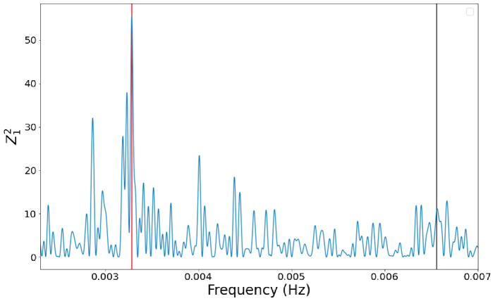
Figure 2: $Z_{1}^{2}$ versus frequency for the XMM-Newton combined MOS1, MOS2, and pn, 0.5-10 keV event list. The red line shows the largest peak at $\sim$304 s, while the black peak shows the location of the 152.49 s period observed in the optical power spectrum by Halpern & Thorstensen (2022).

A periodicity of 152.49$\pm 0.02$ s was observed in the optical light curve of IGR J18434 (Halpern & Thorstensen, 2022). We use the $Z_{1}^{2}$ test (Buccheri et al., 1983) to search for pulsations at this period using the XMM-Newton and NuSTAR event lists. First, we searched for the 152.49 s period using the combined (MOS1+MOS2+pn) event list. The largest peak found in the immediate vicinity (i.e., between $\nu=6.47\times 10^{-3}$ Hz to $\nu=6.64\times 10^{-3}$ Hz or within $\pm 100\sigma$) of the optical period is located at 0.00657 Hz (152.3 s) but has a low $Z_{1}^{2}=11.1$, which is statistically insignificant after accounting for the number of trials. Expanding the search to a larger frequency range ($\nu=0.0005-0.01$ Hz) uncovers a much stronger period ($Z_{1}^{2}=55.6$) at a frequency of $\nu=0.003285\pm 0.000003$ Hz or $P=304.4\pm 0.3$ s, having a False Alarm Probability (FAP) of $\sim$10^-8. The results of the XMM-Newton $Z_{1}^{2}$ test are shown in Figure 2. The uncertainties are estimated by calculating at which frequency $Z^{2}_{\rm 1,max}$ falls to $Z^{2}_{\rm 1,max}-1$. This period is about twice the observed optical period.

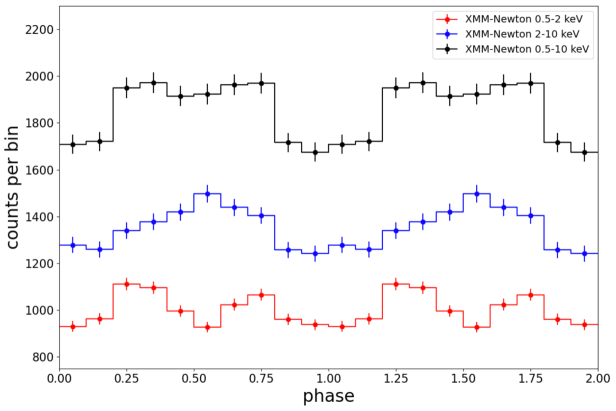
Figure 3: XMM-Newton combined MOS1, MOS2, and pn, 0.5-10 keV pulse profile folded on the pulse period of 304.4 s. Two phases are shown for clarity. The soft and hard band pulse profiles have an arbitrary shift applied for easier comparison between the pulse profiles.

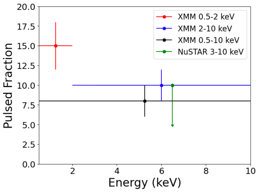
Figure 4: The measured pulsed fraction in several different energy bands. A 3$\sigma$ upper-limit is provided for the NuSTAR non-detection.

The 0.5-10 keV pulse profile shows only one peak per period with a relatively flat top (see Figure 3). We calculate the pulsed fraction, defined as $(C_{\rm max}-C_{\rm min})/(C_{\rm max}+C_{\rm min})$ where $C_{\rm max}$ and $C_{\rm min}$ are the maximum and minimum number of counts in the folded pulse profile, and find a value of $8\pm 2\%$ in the 0.5-10 keV band. We also divided the XMM-Newton pulse profile into soft (0.5-2 keV) and hard (2-10 keV) energy bands (see Figure 3). Interestingly, the pulse profiles are markedly different in these energy ranges, with the soft profile showing two peaks per pulse period, while the hard profile shows only one peak per period. Additionally, the peak of the hard band pulse profile falls in the minimum between the the two peaks seen in the soft band pulse profile. The soft and hard bands have pulsed fractions of $15\pm 3\%$ and $10\pm 2\%$, respectively. The observed pulsed fractions as a function of energy are plotted in Figure 4.

We also searched for the 304.4 s period in the 3-10 keV NuSTAR data. However, we note that at low frequencies, the gaps in the data caused by Earth occultations due to NuSTAR’s low-earth orbit lead to many spurious peaks in the $Z_{1}^{2}$ periodogram related to the harmonics of NuSTAR’s orbital period. Unfortunately one of these harmonics falls very close to the pulse period, making it difficult to determine the significance of the spin period. As a secondary check, we also used the 10 s binned NuSTAR light curve and Stingray (Huppenkothen et al., 2019a, b) to calculate the average power spectra over continuous good time intervals longer than 3 ks, thus removing the power in the harmonics caused by NuSTAR’s orbit. No statistically significant peak is detected at or near the expected pulse frequency. We place a 3$\sigma$ upper-limit on the observed pulsed fraction of $10\%$ in the 3-10 keV energy band.

4 X-ray Spectrum

For spectral analysis we jointly fit the XMM-Newton and NuSTAR data in the 0.5–79 keV range (0.5–12 keV for XMM-Newton and 3–79 keV for NuSTAR) using the XSPEC spectral modeling package (Arnaud, 1996). In order to account for differences in normalization across instruments, we fit each spectral model using a multiplicative constant. The constant for MOS1 was frozen to 1 while the others were allowed to fit freely. Furthermore, tbabs was included in all fits in order to account for ISM absorption. The abundances for the tbabs component may be found in Wilms et al. (2000). For all parameters listed, the errors shown are the $1\sigma$ confidence intervals.

We initially fit both a power-law and a thermal bremsstrahlung model to the IGR J18434 data. However, in both cases, the resulting $\chi_{\rm red}^{2}$ is unacceptably high at 2.4 and 2.5, respectively, for 820 degrees of freedom (dof). In order to improve the bremsstrahlung fit, we included the reflect model described in Magdziarz & Zdziarski (1995). This component modifies the model to account for reflection off of the surface of the WD. While the bremsstrahlung fit was improved by the inclusion of the reflect component, the resulting fit statistic ($\chi_{\rm red}^{2}=1.63$ with 818 dof) was still relatively poor.

Large positive residuals below about 1 keV prompted us to include a partial covering absorption component (pcfabs in XSPEC). Pcfabs is typically included in spectral fitting of IPs (Mukai, 2017). Additionally, positive residuals around 6–7 keV indicate the presence of an Fe line. A Gaussian was added to the model and freely fit to $E_{line}=6.45\pm 0.04$ keV and $\sigma_{line}=0.38\pm 0.06$ keV. This resulted in a $\chi_{\rm red}^{2}$ of 0.95 with 813 dof. Our best-fit model in XSPEC was therefore constant*pcfabs*tbabs*(gaussian+reflect*bremss), the best-fit parameters of which are listed in Table 2. However, the best-fit $\sigma_{line}$ is extraneously large and thus likely includes more than one iron line. Since the $E_{line}$ parameter is fitting to a value larger than 6.4 keV (the energy for a neutral iron fluorescence line), it is likely including the 6.7 keV (He-like) and 6.97 keV (H-like) lines as well. Therefore, we fit the spectrum to the same overall model, but with three separate Gaussian components. The line energy of each Gaussian was frozen to either 6.4, 6.7, or 6.97 keV, and the $\sigma_{line}$ for each component was frozen to 50 eV, as was done in Coughenour et al. (2022). The best-fit parameters for this model are listed in Table 2. The abundance parameter in the reflect model is the abundance of elements heavier than He relative to abundances defined in Wilms et al. (2000). The iron abundance parameter is defined in the same way and was set equal to the general abundance parameter. We froze $rel_{refl}$ to 1.0 in all cases since leaving it as a free parameter resulted in values too high to be physical. The bremsstrahlung temperatures for the single and triple Gaussian fits were not significantly different at $100_{-34}^{+97}$ and $94.4_{-39}^{+29}$ keV, respectively. While the triple Gaussian fit better constrained the bremsstrahlung temperature, it is still high for an IP.

In both bremsstrahlung fits, the best-fit abundance is lower than expected for IPs. To investigate this, we refit the data with a single Gaussian and the abundance frozen to $A=0.5$, more in line with other IPs detected by INTEGRAL (Coughenour et al., 2022). The resulting fit was of similar quality to the previous fits with $\chi_{\rm red}^{2}=0.96$ and 814 dof. The only parameters whose $1\sigma$ confidence intervals did not overlap with those of the original fit were the partial covering fraction ($f=0.68\pm 0.01$) and the bremsstrahlung normalization ($N_{\rm bremss}=1.1\pm 0.1\times 10^{-3}$). Since our results are not affected by these low (and possibly unphysical) abundances, we continue to report our best-fit results hereafter.

Next, we replace the bremsstrahlung model with the “post-shock region" (PSR) model or “ipolar" model from Suleimanov et al. (2016) in order to calculate the WD mass. In addition to the WD mass, this model depends on the magnetospheric radius divided by the radius of the WD, $R_{m}/R_{\rm WD}$. The magnetospheric radius is the point at which the accretion disc is truncated by the WD’s magnetic field. By assuming that $R_{m}$ is equal to the co-rotation radius of the WD, we can set $R_{m}=(\frac{GMP^{2}}{4\pi^{2}})^{1/3}$ where $P$ is the spin period of the WD, which we set to 304.4 s (Suleimanov et al., 2016). $R_{\rm WD}$ can then be calculated using the well-known WD equation of state from Nauenberg (1972) relating WD mass and radius. The $R_{m}$ parameter in the ipolar model can therefore be linked to the mass parameter in XSPEC according to these two equations, as was done in Tomsick et al. (2023) and Coughenour et al. (2022).

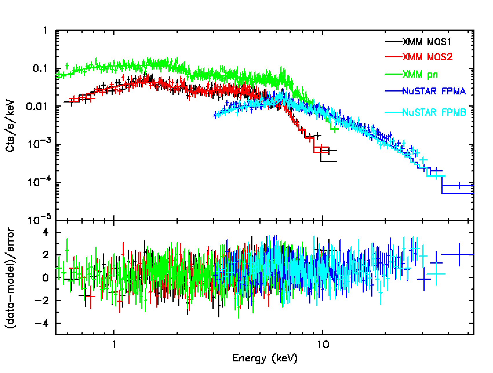
Figure 5: XMM-Newton and NuSTAR joint spectrum (with residuals) fit to the PSR model and three narrow Gaussians. The best-fit parameters for this model are listed in Table 3

The best-fit parameters of the ipolar fit with three Gaussians are displayed in Table 3. The spectrum and corresponding residuals are shown in Figure 5. The best-fit mass was 1.4 $M_{\odot}$, the Chandrasekhar limit and the maximum value allowed in XSPEC. This gives $R_{m}=50.2$ $R_{\rm WD}$. The $1\sigma$ lower limit on the mass was 1.36 $M_{\odot}$. The unabsorbed flux was calculated by applying the cflux convolution model to the additive model components. The full model was therefore constant * pcfabs * tbabs * cflux * (gaussian + gaussian + gaussian + reflect * atable{ipolar.fits}). The energy range for the cflux component was set to 0.5 – 12 keV for the XMM-Newton spectra and 3 – 79 keV for the NuSTAR spectra. Since the cross-normalization constant factors all fit to $\sim$1, the best-fit flux is applicable across instruments. The 0.5 – 12 keV flux is $6.36_{-0.07}^{+0.06}\times 10^{-12}$ erg s^-1 cm^-2. The 3 – 79 keV flux is $1.43_{-0.02}^{+0.01}\times 10^{-11}$ erg s^-1 cm^-2. Assuming a source distance of 3 kpc (Bailer-Jones et al., 2021), these fluxes give luminosities of $6.85\pm 0.07\times 10^{33}$ erg s^-1 and $1.54_{-0.02}^{+0.01}\times 10^{34}$ erg s^-1 in the 0.5 – 12 keV and 3 – 79 keV bands, respectively. The flux in the 17 – 60 keV band is $7.0\pm 0.1\times 10^{-12}$ erg s^-1 cm^-2 as compared to $5.2\pm 0.8\times 10^{-12}$ erg s^-1 cm^-2 reported in Tomsick et al. (2021) as measured by INTEGRAL.

Again, the best-fit abundance for the ipolar fit with three Gaussians is smaller than expected. We try the same procedure as before, refitting the data with abundance frozen to $A=0.5$. This fit gave a $\chi_{\rm red}^{2}=0.98$ and 814 dof. The parameters whose $1\sigma$ confidence intervals did not overlap with those displayed in Table 3 were $N_{\rm H,pc}=6.2\pm 0.5\times 10^{22}$ cm^-2, the partial covering fraction $=0.70\pm 0.01$, and $\cos i=0.3\pm 0.1$. Although the 1$\sigma$ upper limit on the mass reached 1.4 $M_{\odot}$, the mass was best fit to 1.36 $M_{\odot}$with a lower bound of 1.33 $M_{\odot}$.

5 Discussion

The classification of IGR J18434 determined by Tomsick et al. (2021) is supported by the above spectral analysis due to its spectra being well fit to the PSR model. Furthermore, the detection of a strong iron complex in the 6–7 keV range is consistent with the X-ray properties of IPs, as is the detection of a spin period in the optical and X-ray bands.

Based on time-series photometry conducted by Halpern & Thorstensen (2022), a signal in the optical power spectrum of IGR J18434 was found at $152.49\pm 0.02$ s. Through the X-ray timing analysis described in Section 3, we find a period of $P=304.4\pm 0.3$ s, nearly twice the previously reported signal. We therefore conclude that $P=304.4\pm 0.3$ s is the true WD spin period, and that the $152.49\pm 0.02$ s signal is a harmonic of the fundamental period. It is fairly common for the initially discovered period to turn out to be a harmonic rather than the fundamental frequency. For example, in the case of the IP V2306 Cygni (WGA J1958.2+3232), observations from both ASCA and the Astrophysical Observatory of Catania (OACT) observed a period of about 733 s (Israel et al., 1998; Uslenghi et al., 2000). However, OACT also observed a peak in the periodograms at 1466 s, twice the previously noted period.

Norton et al. (1999) describes how two-pole accretion does not exclusively lead to a double-peaked pulse profile. Instead, two-pole accretion may lead to either a single or double-peaked pulse profile, depending on the strength of the white dwarf’s magnetic field. If the magnetic field is weak, material travels along the field lines beginning closer to the surface of the WD. This produces a larger accretion region, and thus the optical depth across the accretion column can be greater than the optical depth up the accretion column. Therefore, a double peaked profile will be produced since there will be a maximum in received flux at the two observing points that align with the magnetic field lines. This double peaked effect, according to Norton et al. (1999), is predominantly seen in IPs with a WD spin period less than $\sim$700 s, as is the case for IGR J18434. The idea that the accretion disc is truncated close to the WD surface seems to contradict our finding that $R_{m}=50.2$ $R_{\rm WD}$. However, given how massive IGR J18434 is, the WD is extremely compact leading to a higher $R_{m}/R_{\rm WD}$. It may therefore be the case that the absolute value of $R_{m}$ is more significant to the pulse profile shape than the ratio of $R_{m}$ to $R_{\rm WD}$. While a double peak is observed in the 0.5 – 2 keV XMM-Newton pulse profile, only a single peak is observed in the 2 – 10 keV band. This difference in pulse profiles may be due to the fact that, although the geometric effects are similar at both energies, the photoelectric absorption varies.

We can use the best-fit $R_{m}$ to estimate $\dot{M}$, the mass accretion rate and $B$, the surface magnetic field at the accretion region. We use the formula, $L=GM\dot{M}(\frac{1}{R}-\frac{1}{R_{m}})$ and $L=1.45\times 10^{34}$ erg s^-1to find $\dot{M}=1.3\times 10^{16}$ g/s. We then use this value to calculate $B$ using equation 8 in Suleimanov et al. (2019) which assumes $R_{m}$ is proportional to the Alfvén radius ($R_{m}=\Lambda R_{A}$). Assuming $\Lambda=0.5$ (as is done in Suleimanov et al. (2019)), we find $B=94$ MG. If we use the lower bound value on the best-fit mass ($M=1.36M_{\odot}$), we find $R_{m}=34.9$ $R_{\rm WD}$ and $B=39$ MG. We also use equation 3 in Norton & Watson (1989) to calculate the magnetic moment, $\mu=1.6\times 10^{32}$ G cm³. Here, we have assumed $\phi=1$, or that the magnetosphere is spherically symmetric.

The estimated magnetic moment of IGR J18434, $\mu=1.6\times 10^{32}$ G cm³, given $M=1.36$ $M_{\odot}$, is consistent with the range of expected values ($10^{32-33}$ G cm³) found by Norton et al. (2004) for most IPs. Polars, in contrast, generally have higher WD magnetic moments ($\mu\stackrel{{\scriptstyle>}}{{\sim}}10^{33}$ G cm³). However, Norton et al. (2004) suggests that low magnetic moment systems (such as IGR J18434) may still evolve to polars given a long orbital period ($P_{\rm orb}>3$ hr). Follow-up observations confirming the orbital period of IGR J18434 could therefore be useful in determining its evolution.

It is possible that the 3 hour peak observed in the NuSTAR and XMM-Newton light curves is the orbital period. The large modulation due to this potential orbital period is evident in the XMM-Newton light curves shown in Figure 1. However, the length of the observation only spans $\sim$2.1 times this period, so this candidate period should be verified through additional observations. If this is the true orbital period though, it would be comparable to that of the IP BG CMi which has an orbital period of $\sim$3.25 hr (de Martino et al., 1995). Parker et al. (2005) suggests that orbital modulation in IPs is due to photoelectric absorption at the accretion disc. Parker et al. (2005) predicts that the inclination angle required for orbital modulation to be seen is greater than $60^{\circ}$. According to our spectral modeling, the angle between our line of sight and the accretion column is $\cos i>0.60$ or $i\lower 2.15277pt\hbox{$\;\buildrel<\over{\sim}\;$}50^{\circ}$. There may therefore be a misalignment between the accretion column and the normal to the orbital plane. However, Mukai et al. (2015) discusses the degeneracy between the angle of the accretion column and the reflection amplitude, which makes it difficult to determine either parameter through spectral analysis alone.

The continued detection of high mass WDs by INTEGRAL such as IGR J14091-6108, IGR J18007-4146, and IGR J15038-6021 (Tomsick et al. (2016); Coughenour et al. (2022); Tomsick et al. (2023)) may indicate that WDs in CVs gain mass throughout accretion-nova cycles. Simulations of high mass WDs ($M>0.6$ $M_{\odot}$) by Starrfield et al. (2020) found that these WDs can accrete more mass than they lose via classical novae events. Once a WD gains enough mass to reach the Chandrasekhar limit ($\sim$1.4 $M_{\odot}$), they may lead to Type Ia supernovae, significant for their role in cosmology as standard candles. Another possible solution to the WD mass problem is that low mass WDs in CVs lose angular momentum and merge with their donor stars, leaving a greater number of CVs with higher mass WDs to be observed (Schreiber et al., 2016).

Due to its high energy band, INTEGRAL is exceptionally well equipped to search for high mass IPs. Figure 6 shows the WD masses and spin periods of various IPs as measured by Shaw et al. (2020), Suleimanov et al. (2019), Ritter & Kolb (2011), de Martino et al. (2020), and our studies of IGR sources. INTEGRAL’s ability to detect high mass IPs is illustrated in Figure 6 where the three IPs with masses closest to the Chandrasekhar limit are those detected by INTEGRAL.

Data Availability

Data used in this paper are available through NASA’s HEASARC.

Table 1: Details of Observations of IGR J18434

Observatory	ObsID	Instrument	Start Time (UT)	End Time (UT)	Exposure (ks)
XMM-Newton	0890620201	MOS1	2022 March 12, 16:57:00	2022 March 13, 00:20:00	25.7
"	"	MOS2	"	"	26.0
"	"	pn	"	"	18.3
NuSTAR	30760002002	FPMA	2022 March 12, 15:16:09	2022 March 13, 15:16:09	40.2
"	"	FPMB	"	"	39.8

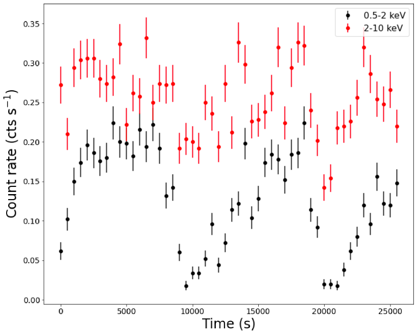
Figure 1: XMM-Newton EPIC pn 0.5-2 (black) and 2-10 (red) keV light curves with a 500 s binning. Variability is seen in both light curves, but is much more visible in the soft light curve.

Table 2: Spectral results for Bremsstrahlung model fits

Parameter	Units	1 Gaussian	3 Gaussians
$N_{\rm H}$	$10^{22}$ cm-2	$0.17_{-0.02}^{+0.05}$	$0.17_{-0.02}^{+0.06}$
$N_{\rm H,pc}$	$10^{22}$ cm-2	$4.7_{-0.4}^{+1.0}$	$5.46_{-1.2}^{+0.95}$
pc fraction	—	$0.52_{-0.01}^{+0.03}$	$0.53\pm 0.04$
$E_{\rm line1}$	keV	$6.45\pm 0.04$	$6.4$
$\sigma_{\rm line1}$	keV	$0.38\pm 0.06$	$0.05^{d}$
$N_{\rm line1}$	ph cm-2 s-1	$(2.66_{-0.29}^{+0.23})\times 10^{-5}$	$(1.24\pm 0.1)\times 10^{-5}$
$EW_{\rm line1}$	eV	$505_{-55}^{+43}$	$212\pm 17$
$E_{\rm line2}$	keV	—	$6.7^{d}$
$\sigma_{\rm line2}$	keV	—	$0.05^{d}$
$N_{\rm line2}$	ph cm-2 s-1	—	$(0.4\pm 0.1)\times 10^{-5}$
$EW_{\rm line2}$	eV	—	$53_{-13}^{+14}$
$E_{\rm line3}$	keV	—	$6.97^{d}$
$\sigma_{\rm line3}$	keV	—	$0.05^{d}$
$N_{\rm line3}$	ph cm-2 s-1	—	$(0.4\pm 0.1)\times 10^{-5}$
$EW_{\rm line3}$	eV	—	$72\pm 18$
$rel_{\rm refl}$	—	1.0d	1.0d
$A$	—	$0.007_{-0.003}^{+0.09}$	$0.006_{-0.003}^{+0.15}$
$A_{\rm Fe}$	—	$0.007$	$0.006$
$\cos{i}$	—	$0.75_{-0.5}^{+0.1}$	$>0.28$
$kT$	keV	$100.0_{-34}^{+97}$	$94.4_{-39}^{+29}$
$N_{\rm bremss}$	—	$(6.4^{+0.5}_{-0.2})\times 10^{-4}$	$(6.3_{-0.6}^{+0.4})\times 10^{-4}$
CMOS1	—	1.0d	1.0d
CMOS2	—	$0.97\pm 0.02$	$0.97\pm 0.02$
Cpn	—	$0.99\pm 0.02$	$0.99\pm 0.02$
CFPMA	—	$1.19_{-0.02}^{+0.03}$	$1.18\pm 0.03$
CFPMB	—	$1.20\pm 0.03$	$1.19\pm 0.03$
$\chi_{\rm\nu}^{2}/$(dof)	—	0.95(813)	0.96(813)

Table 3: Spectral results for PSR model fit

Parameter	Units	PSR Model
$N_{\rm H}$	$10^{22}$ cm-2	$0.20_{-0.02}^{+0.03}$
$N_{\rm H,pc}$	$10^{22}$ cm-2	$4.46_{-0.7}^{+0.9}$
pc fraction	—	$0.56_{-0.03}^{+0.04}$
$E_{\rm line1}$	keV	$6.4$
$\sigma_{\rm line1}$	keV	$0.05^{c}$
$N_{\rm line1}$	ph cm-2 s-1	$(1.2\pm 0.1)\times 10^{-5}$
$EW_{\rm line1}$	eV	$204\pm 17$
$E_{\rm line2}$	keV	$6.7^{c}$
$\sigma_{\rm line2}$	keV	$0.05^{c}$
$N_{\rm line2}$	ph cm-2 s-1	$(0.38\pm 0.1)\times 10^{-5}$
$EW_{\rm line2}$	eV	$51_{-13}^{+14}$
$E_{\rm line3}$	keV	$6.97^{c}$
$\sigma_{\rm line3}$	keV	$0.05^{c}$
$N_{\rm line3}$	ph cm-2 s-1	$(0.36\pm 0.1)\times 10^{-5}$
$EW_{\rm line3}$	eV	$65_{-18}^{+19}$
$rel_{\rm refl}$	—	1.0c
$A$	—	$0.02\pm 0.01$
$A_{\rm Fe}$	—	$0.02$
$\cos{i}$	—	$>0.60$
$M_{\rm WD}$	$M_{\odot}$	$>1.36$
$R_{\rm m}$	$R_{\rm WD}$	50.2
$N_{\rm PSR}$	—	$(2.88^{+5}_{-0.2})\times 10^{-30}$
CMOS1	—	1.0c
CMOS2	—	$0.97\pm 0.02$
Cpn	—	$0.99\pm 0.02$
CFPMA	—	$1.18\pm 0.03$
CFPMB	—	$1.19\pm 0.03$
$\chi_{\rm\nu}^{2}/$(dof)	—	0.96(813)

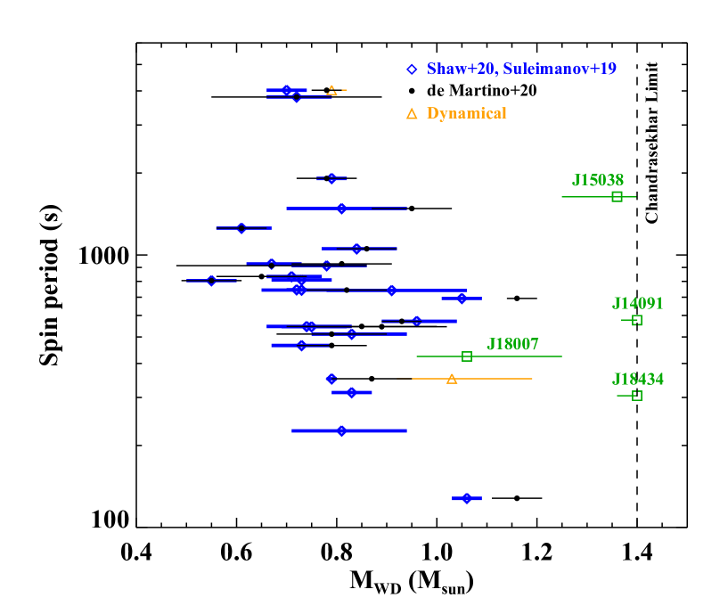
Figure 6: Plot of WD masses and spin periods of IPs. This graph is Figure 10 from Tomsick et al. (2023) with data from IGR J18434 included. The IPs marked in green are from our studies of IGR sources: J14091 (Tomsick et al., 2016), J18007 (Coughenour et al., 2022), J15038 (Tomsick et al., 2023), and J18434 (this work).

References

- Arnaud (1996) Arnaud, K. A. 1996, in Astronomical Society of the Pacific Conference Series, Vol. 101, Astronomical Data Analysis Software and Systems V, ed. G. H. Jacoby & J. Barnes, 17
- Bailer-Jones et al. (2021) Bailer-Jones, C. A. L., Rybizki, J., Fouesneau, M., Demleitner, M., & Andrae, R. 2021, VizieR Online Data Catalog, I/352
- Bird et al. (2010) Bird, A. J., Bazzano, A., Bassani, L., et al. 2010, ApJS, 186, 1, doi: 10.1088/0067-0049/186/1/1
- Bird et al. (2016) Bird, A. J., Bazzano, A., Malizia, A., et al. 2016, ApJS, 223, 15, doi: 10.3847/0067-0049/223/1/15
- Buccheri et al. (1983) Buccheri, R., Bennett, K., Bignami, G. F., et al. 1983, A&A, 128, 245
- Coughenour et al. (2022) Coughenour, B. M., Tomsick, J. A., Shaw, A. W., et al. 2022, MNRAS, 511, 4582, doi: 10.1093/mnras/stac263
- de Martino et al. (2020) de Martino, D., Bernardini, F., Mukai, K., Falanga, M., & Masetti, N. 2020, Advances in Space Research, 66, 1209, doi: 10.1016/j.asr.2019.09.006
- de Martino et al. (1995) de Martino, D., Mouchet, M., Bonnet-Bidaud, J. M., et al. 1995, A&A, 298, 849
- Gaia Collaboration et al. (2021) Gaia Collaboration, Brown, A. G. A., Vallenari, A., et al. 2021, A&A, 649, A1, doi: 10.1051/0004-6361/202039657
- Halpern & Thorstensen (2022) Halpern, J. P., & Thorstensen, J. R. 2022, ApJ, 924, 67, doi: 10.3847/1538-4357/ac2f9f
- Hare et al. (2021) Hare, J., Halpern, J. P., Tomsick, J. A., et al. 2021, ApJ, 914, 85, doi: 10.3847/1538-4357/abfa96
- Harrison et al. (2013) Harrison, F. A., Craig, W. W., Christensen, F. E., et al. 2013, ApJ, 770, 103, doi: 10.1088/0004-637X/770/2/103
- Huppenkothen et al. (2019a) Huppenkothen, D., Bachetti, M., Stevens, A. L., et al. 2019a, ApJ, 881, 39, doi: 10.3847/1538-4357/ab258d
- Huppenkothen et al. (2019b) Huppenkothen, D., Bachetti, M., Stevens, A., et al. 2019b, Journal of Open Source Software, 4, 1393, doi: 10.21105/joss.01393
- Israel et al. (1998) Israel, G. L., Angelini, L., Campana, S., et al. 1998, MNRAS, 298, 502, doi: 10.1046/j.1365-8711.1998.01653.x
- Krivonos et al. (2022) Krivonos, R. A., Sazonov, S. Y., Kuznetsova, E. A., et al. 2022, MNRAS, 510, 4796, doi: 10.1093/mnras/stab3751
- Krivonos et al. (2017) Krivonos, R. A., Tsygankov, S. S., Mereminskiy, I. A., et al. 2017, MNRAS, 470, 512, doi: 10.1093/mnras/stx1276
- Krivonos et al. (2017) Krivonos, R. A., Tsygankov, S. S., Mereminskiy, I. A., et al. 2017, Monthly Notices of the Royal Astronomical Society, 470, 512, doi: 10.1093/mnras/stx1276
- Krivonos et al. (2021) Krivonos, R. A., Bird, A. J., Churazov, E. M., et al. 2021, New Astron. Rev., 92, 101612, doi: 10.1016/j.newar.2021.101612
- Lucas et al. (2008) Lucas, P. W., Hoare, M. G., Longmore, A., et al. 2008, MNRAS, 391, 136, doi: 10.1111/j.1365-2966.2008.13924.x
- Lutovinov et al. (2020) Lutovinov, A., Suleimanov, V., Manuel Luna, G. J., et al. 2020, New Astronomy Reviews, 91, 101547, doi: https://doi.org/10.1016/j.newar.2020.101547
- Magdziarz & Zdziarski (1995) Magdziarz, P., & Zdziarski, A. A. 1995, MNRAS, 273, 837, doi: 10.1093/mnras/273.3.837
- Mukai (2017) Mukai, K. 2017, PASP, 129, 062001, doi: 10.1088/1538-3873/aa6736
- Mukai et al. (2015) Mukai, K., Rana, V., Bernardini, F., & de Martino, D. 2015, ApJ, 807, L30, doi: 10.1088/2041-8205/807/2/L30
- Nauenberg (1972) Nauenberg, M. 1972, ApJ, 175, 417, doi: 10.1086/151568
- Norton et al. (1999) Norton, A. J., Beardmore, A. P., Allan, A., & Hellier, C. 1999, A&A, 347, 203, doi: 10.48550/arXiv.astro-ph/9811310
- Norton & Watson (1989) Norton, A. J., & Watson, M. G. 1989, MNRAS, 237, 715, doi: 10.1093/mnras/237.3.715
- Norton et al. (2004) Norton, A. J., Wynn, G. A., & Somerscales, R. V. 2004, The Astrophysical Journal, 614, 349, doi: 10.1086/423333
- Parker et al. (2005) Parker, T. L., Norton, A. J., & Mukai, K. 2005, A&A, 439, 213, doi: 10.1051/0004-6361:20052887
- Pecaut & Mamajek (2013) Pecaut, M. J., & Mamajek, E. E. 2013, ApJS, 208, 9, doi: 10.1088/0067-0049/208/1/9
- Ritter & Kolb (2011) Ritter, H., & Kolb, U. 2011, VizieR Online Data Catalog, B/cb
- Schreiber et al. (2016) Schreiber, M. R., Zorotovic, M., & Wijnen, T. P. G. 2016, MNRAS, 455, L16, doi: 10.1093/mnrasl/slv144
- Shaw et al. (2020) Shaw, A. W., Heinke, C. O., Mukai, K., et al. 2020, MNRAS, 498, 3457, doi: 10.1093/mnras/staa2592
- Starrfield et al. (2020) Starrfield, S., Bose, M., Iliadis, C., et al. 2020, ApJ, 895, 70, doi: 10.3847/1538-4357/ab8d23
- Suleimanov et al. (2016) Suleimanov, V., Doroshenko, V., Ducci, L., Zhukov, G. V., & Werner, K. 2016, A&A, 591, A35, doi: 10.1051/0004-6361/201628301
- Suleimanov et al. (2019) Suleimanov, V. F., Doroshenko, V., & Werner, K. 2019, MNRAS, 482, 3622, doi: 10.1093/mnras/sty2952
- Tomsick et al. (2016) Tomsick, J. A., Rahoui, F., Krivonos, R., et al. 2016, MNRAS, 460, 513, doi: 10.1093/mnras/stw871
- Tomsick et al. (2021) Tomsick, J. A., Coughenour, B. M., Hare, J., et al. 2021, The Astrophysical Journal, 914, 48, doi: 10.3847/1538-4357/abfa1a
- Tomsick et al. (2023) Tomsick, J. A., Kumar, S. G., Coughenour, B. M., et al. 2023, Monthly Notices of the Royal Astronomical Society, 523, 4520, doi: 10.1093/mnras/stad1729
- Uslenghi et al. (2000) Uslenghi, M., Bergamini, P., Catalano, S., Tommasi, L., & Treves, A. 2000, A&A, 359, 639, doi: 10.48550/arXiv.astro-ph/0005460
- Wilms et al. (2000) Wilms, J., Allen, A., & McCray, R. 2000, ApJ, 542, 914, doi: 10.1086/317016