D’OH: Decoder-Only random Hypernetworks
for Implicit Neural Representations

Abstract

Deep implicit functions have been found to be an effective tool for efficiently encoding all manner of natural signals. Their attractiveness stems from their ability to compactly represent signals with little to no off-line training data. Instead, they leverage the implicit bias of deep networks to decouple hidden redundancies within the signal. In this paper, we explore the hypothesis that additional compression can be achieved by leveraging the redundancies that exist between layers. We propose to use a novel run-time decoder-only hypernetwork – that uses no offline training data – to better model this cross-layer parameter redundancy. Previous applications of hyper-networks with deep implicit functions have applied feed-forward encoder/decoder frameworks that rely on large offline datasets that do not generalize beyond the signals they were trained on. We instead present a strategy for the initialization of run-time deep implicit functions for single-instance signals through a Decoder-Only randomly projected Hypernetwork (D’OH). By directly changing the dimension of a latent code to approximate a target implicit neural architecture, we provide a natural way to vary the memory footprint of neural representations without the costly need for neural architecture search on a space of alternative low-rate structures.

1 Introduction

Implicit neural representations, also known as coordinate networks, have received attention for their ability to represent signals from different domains – including sound, images, video, sign distance fields, and neural radiance fields – all within a single generalized framework [74, 87, 56, 22, 57, 16]. When combined with quantization strategies, they act as a neural signal compressor which can be applied generally across different modalities; most notably in Compressed Implicit Neural Representations (COIN) of Dupont et al [22]. Combining this with lossless entropy compressors can lead to further memory reductions [76, 22, 68, 33, 19]

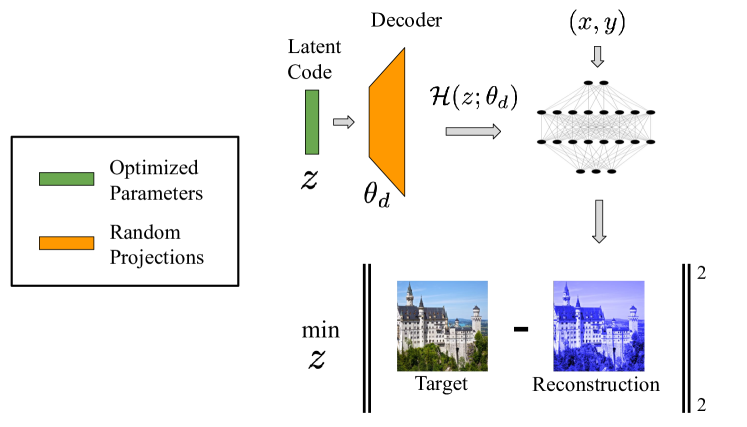
Figure 1: We propose a decoder-only hypernetwork that optimises a low-dimensional latent code to directly generate the weights of a target implicit neural representation. This framework is data modality agnostic and requires no offline training data. Instead only the target network architecture and target data instance are needed. We use random projections as a network decoder enabling a highly compact code representation.

Neural networks are believed to contain significant redundancy in parameterization, motivating interest in the use of more compact architectures [21, 34, 36, 38, bubeck_universal_2022, 32]. A prominent example is hypernetworks - a metanetwork that generates the weights of a target network [34, 14]. As generating functions can contain fewer parameters than a target network, hypernetwork can be a compact way of approximating the performance of a more expressive architecture [26, 34]. Frequently, hypernetworks are task-conditioned on a target signal class or application offline - for example, in compression, super-resolution, inpainting, or style transfer [5, 58, 43, 14]. These generating functions are regularly more complex than the target architecture - and may include mixtures of convolutional layers, transformers, graph neural networks, and so on [14]. By conditioning on training data, these hypernetworks are able to generate new networks for a target class of signals. However, this is at the cost of compactness and generalisation to out-of-distribution data instances – two of the primary motivations for the use of implicit neural representations.

To now the use of hypernetworks in implicit neural representations has exclusively focused on the task-conditioned encoder-decoder type (in which data instances are inputs to a hypernetwork outputting an implicit neural representation). In contrast, we suggest that a decode-only form of hypernetwork is possible in which the data instance appears only as a target output. Rather than requiring offline training on the target signal class this decode-only architecture is optimised directly to predict a given data instance by projecting to a target implicit neural network structure. Similar to the training of standard implicit neural representations this requires no offline datasets and can be optimised at runtime [48, 62, 22]. By design, we set the latent parameters of this hypernetwork to be fewer than the target network architecture, enabling a highly compact representation. We explore a special decode-only structure, which involves a low-dimensional parameter vector projected by a fixed linear random mapping to construct the target network. In contrast to existing implicit neural representation methods such as COIN [22, 76], which require neural architecture search on low-rate architectures to achieve superior performance, we show that we can control bit-rate by directly changing the latent code dimension.

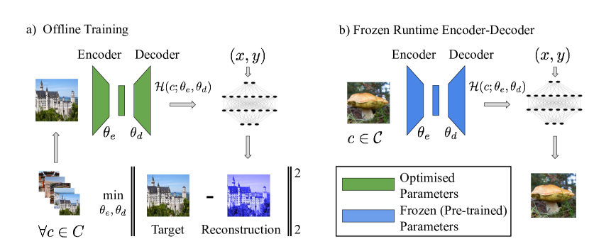
Figure 2: A conventional Encoder-Decoder Hypernetwork is pre-trained on a class of signals to predict the weights of an implicit neural representation when fed a target signal at runtime. This is advantageous to condition on a target signal class or task, but comes at the cost of generality to out-of-distribution signals. In contrast, in this paper we propose the use Decoder-Only Hypernetworks (see: Figure 1) which can be trained at runtime using only the target signal and are free of external data.

We make the following contributions in this paper:

• We introduce a novel hypernetwork framework (D’OH - Decoder-Only random Hypernetworks) for runtime optimization of implicit neural representations which requires only the target signal instance, with no need for offline preconditioning on a training set of the target signal class.

• We provide an example decoder-only hypernetwork architecture based on a trainable latent code vector and fixed random projection decoder weights. As only the latent code, biases, and an integer seed need to be communicated we show this is applicable to data compression.

• We derive a novel initialization for this hypernetwork to match the layer weight variances of SIREN networks, that modifies the distribution of the non-trainable random weights rather than the learned parameters.

2 Background and Motivation

2.1 Implicit Neural Representation Compression

An implicit neural representation (INR) is a parameterised function $f_{\psi}(\textbf{x})\to\textbf{y}$ mapping coordinates x to features y, trained to closely approximate a target signal $g$ such that $\|f_{\psi}(\textbf{x})-g(\textbf{x})\|\leq\epsilon$. INRs have been widely applied to represent signal types including images, sound, neural radiance fields, and sign distance fields [74, 57, 87, 52, 56, 76, 23]. Implicit representations have garnered significant interest for their potential in compressing signals. This involves a neural network trained to implicitly predict a single signal instance, such as an image, video, or sound wave. Applying a forward pass of the training network produces a lossy reconstruction of the original signal [22, 23, 76, 19]. Further compression can be achieved by exploiting the high-degree of redundancy known to exist in neural network weights [36, 21, 54, 34]. For example, quantizing network weights [22, 23, 76, 52, 73, 18, 19], pruning [18, 47], inducing sparse network structures [89, 67], neural architecture search, variational methods [68], hash-tables [78, 79], latent transformations [91, 46, 42] and entropy compression [76, 23, 33, 46, 42].

2.2 Hypernetworks

Hypernetworks are a type of meta-network that generates the parameters for another network, typically referred to as the target network [14]. As proposed by Ha et al. [34] is often achieved by approximating the target network’s architecture with a low-dimensional latent code. Hypernetworks take the form of a generating function:

$$\mathcal{H}_{\theta}(z)=\psi$$ (1)

where $z$ is a latent code and $\psi$ refers to the generated parameters of a target network function $f_{\psi}$. For notational simplicity, we use $W_{l}$ to refer to weights of the $l^{th}$ layer of a $L$-layer multi-layer perceptron, and $\psi$ to refer to the parameters involved in a more generic mapping. Hypernetworks have been applied to various use-cases [14], including compression [27, 41, 58], neural architecture search [90], image super-resolution [43, 82] and sound generation [77]. There is no single dominant architecture used to generate hypernetworks and a wide number of architectures have been used in practice, including transformers; convolutional, recurrent, residual, and convolutional networks; generative adversarial networks, graph networks, and kernel networks [17, 34, 27, 70, 71, 90, 14]. Hypernetworks have recently been explored for use within implicit neural representations, with many works using the network to precondition on a task or domain for use on new data instances or for downstream tasks [14]. This includes volume rendering [85], super-resolution of images [43, 85] and hyperspectral images [92], sound [77], novel view synthesis [85, 15, 69], and partial-differential equations [10, 53].

2.3 Encoder-Decoder Hypernetworks

Hypernetworks as currently applied to implicit neural representations have been of an encoder-decoder type, where a training set drawn from the target signal class is used to train a hypernetwork before being evaluated on the target signal instance. Given a class $\mathcal{C}$ of a signal type, a training set $C\in\mathcal{C}$ with samples $c\in C$ is used to train a hypernetwork $\mathcal{H}(c;\theta_{e},\theta_{d})$ to generate the weights $\psi$ of the implicit neural function $f_{\psi}(x)$ where $x$ is the input coordinate. The network is optimized offline to minimise the loss $\sum_{x}\|f_{\psi}(x)-c(x)\|^{2}_{2}$ across the training set, thereby learning implicit regularities of the signal class. At runtime the hypernetwork is used to generate the weights for an unseen data instance in the target class $c\in\mathcal{C},c\notin C$ which may be used for a downstream task. Note that we are being general with hypernetwork architecture, and have used $\theta_{e},\theta_{d}$ to collectively define the parameters of the encoding (learning from data instance) and decoding (generating parameters to the target architecture) functions of the hypernetwork. In practice, these are often intermingled, as in a MLP where the output layer directly generates network weights and is itself involved in learning the encoding; however, in complicated architectures or multi-step processes the two parameter sets may be more distinctly separated [14]. For example, a hypernetwork applied to image super-resolution may be trained on an image dataset such as the DIV2K before being evaluated on other datasets, as in [43]. In [74], the authors use a hypernetwork to produce a SIREN MLP for image inpainting, in which the hypernetwork is conditioned on a subset of the CelebA database [28, 50]. [92] condition on a set of hyperspectral images to generate a target MLP. HyperSound conditions on the VCTK dataset for generating audio INRs [77]. While not directly using a hypernetwork, several related works have sought to condition a base network on target class data through metalearning techniques such as MAML [25], before using this as an initialization for fine-tuning, autoencoding, or learning a set of modulations for a novel data instance [68, 23, 76, 80, 61].

2.4 Decoder-Only Hypernetworks

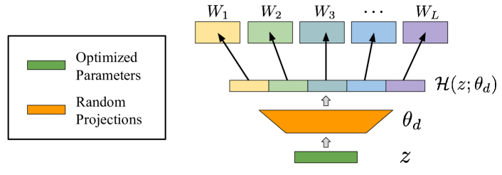
Figure 3: Weight generation in a decoder-only hypernetwork. Latent code $z$ and decoding parameters $\theta_{d}$ are used to construct a vectorized version of the hypernetwork output $\mathcal{H}(z;\theta_{d})$. For our purposes we investigate on the special case where $\mathcal{H}(z;\theta_{d})=B_{l}z$ where $B_{l}$ is a fixed and untrained per-layer random weight matrix.

While in Encoder-Decoder Hypernetworks the goal is to learn a domain-conditioned hypernetwork mapping to the target network, we instead propose to learn a latent code at runtime directly from the target data itself. As this process does not involve a separate encoding step of domain information to the latent space, we describe this as a ‘decoder-only hypernetwork’ in which the latent code is optimized runtime by projecting to the target network. The decoder-only hypernetwork is denoted as $\mathcal{H}(z;\theta_{d})\to\psi$. For our purposes we restrict ourselves to the situation in which the decoder parameters $\theta_{d}$ are fixed and only the latent code $z$ is learned. As a specific example, we focus on a $L$-layer multi-layer perceptron target network and set the decoding weights to simply be linear maps $\theta_{d}:=\{B_{l}\}_{l=1}^{L}$ defined by a family of fixed random matrices $B_{l}$: one for each layer. The target network weights $W_{l}$ for the $l^{th}$ layer are then defined to be the image of the latent vector $z\in\mathbb{R}^{n}$ under the linear map $B_{l}$. We maintain a separate trainable bias term $h_{l}$ for each layer in the target network. Denoting $\bar{W}_{l}$ as the generated vectorized form of $W_{l}$ Equation (1) reduces to:

$$\mathcal{H}_{\theta}(z)=\{\bar{W}_{l}\}_{l=1}^{L}=\{B_{l}z\}_{l=1}^{L}.$$ (2)

This minimal architecture ensures maximal compression through the use of depth-wise redundancy in a target use-case of signal compression, however more general decoder-only architectures could include more expressive latent variables (for example per-layer latent variables $z_{l}$) or different decoding functions. The auto-decoder approach of [60] can be considered one such example using a fully-parameterised decoder. The linear random projection approach we have described induces parameter sharing [59, 81, 66, 14], in which learned parameters are tied by arbitrary sampled random matrices. The choice of random embeddings is motivated by the effective use of random matrices in the low-rank matrix decompositions described by Denil et al. [21], classical results in the use of random projections for dimension reduction [12, 20, 35, 40, 86], and recent works exploring the compressibility of neural architectures using random projections [44, 6, 3, 63, 55].

2.5 Hypernetwork Training and Initialization

Initializing hypernetworks is non-trivial, as standard schemes such as those by Glorot [31] and He [37] do not directly apply due to the unique challenges posed by potential exploding or vanishing gradients when target network weights are generated by a hypernetwork [13]. Even with infinite-width hypernetworks, one cannot guarantee convergence when approximating a modestly-sized target network [49]. Chang et al. explore initialization strategies for hypernetworks to maintain layer variances in tanh and ReLU target networks by modifying the variance of parameters in the generating network [13]. However, implicit neural representations, which more frequently involve the use of alternative non-linearities such as the sine activation function [74], require a different approach While [74] explore a one-layer ReLU MLP for as an encoder-decoder hypernetwork to generate weights for SIREN, this does not translate to the architecture described in Equation (2), necessitating a modified initialization scheme.

2.5.1 D’OH Equivalent Initialization

We control the initialization of the projected weight matrices by changing the variance of the random matrices $\{B_{l}\}_{l=1}^{L}$ used to map the generating latent vector to the target network weights. It can be shown that where entries of $z$ are drawn from a distribution $\text{Var}(z)$ that the variance of each $B_{l}$:

$$\text{Var}(B_{l})=\frac{\text{Var}(\bar{W}_{l})}{n\text{Var}(z)}.$$ (3)

We initialize the matrices $\{B_{l}\}_{l=1}^{L}$ such that the projected weight matrices will have have identically distributed entries of the same variance as in the original SIREN implementation [74]. We initialise the latent code uniformly between $[-1/n,1/n]$. Biases are not tied to the generating vector and are separately initialized to zero, with the exception of the output bias which is set to 0.5 as the middle of the tested signals output range $[0,1]$.

2.5.2 Neural Architecture Search

One of the difficulties of using implicit neural representations for compression is the need to search across different architectures to achieve changes in bit-rates. In the COIN this is handled by performing Neural Architecture Search [24, 84, 22]. MLP architectures (width, hidden) that satisfy a bits-per-pixel (BPP) target (e.g. 0.3) on the Kodak dataset [2] are searched over with the best performing models at each bit-rate selected for further experiments. Figure 4 shows that this is useful, as architectures show variability in performance. However this search is potentially costly, due to the time needed to train each model and the large number of satisfying architectures. This extends considerably if considering different quantization levels (e.g. for quantization aware training) as in [76, 33, 19]. In contrast, by working with a fixed target architecture generated by a decoder-only hypernetwork we can control the desired bit-rate by directly varying a latent code dimension. This avoids the need to search across alternative networks to achieve lower bit-rates.

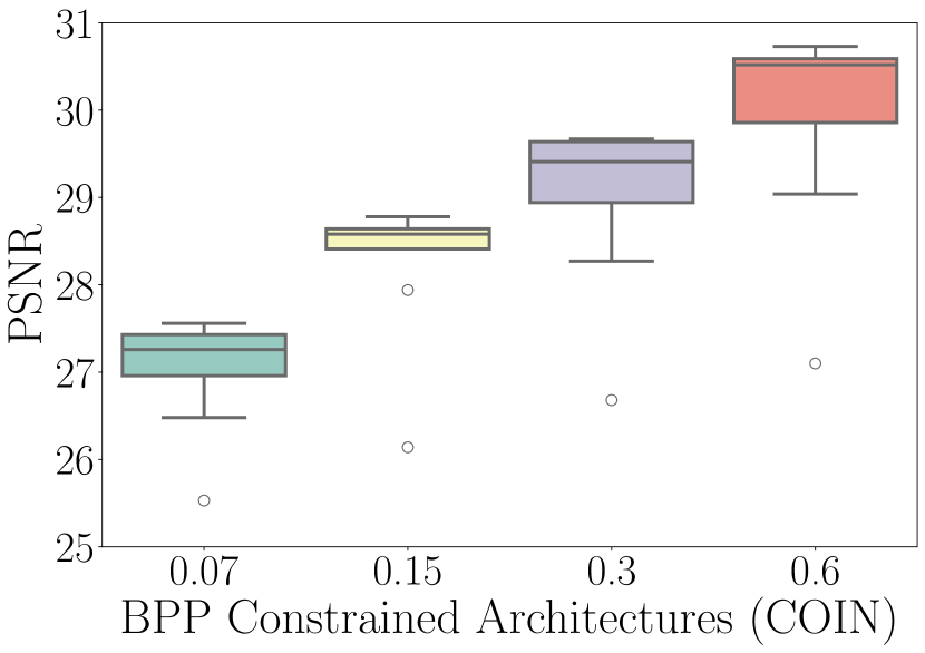
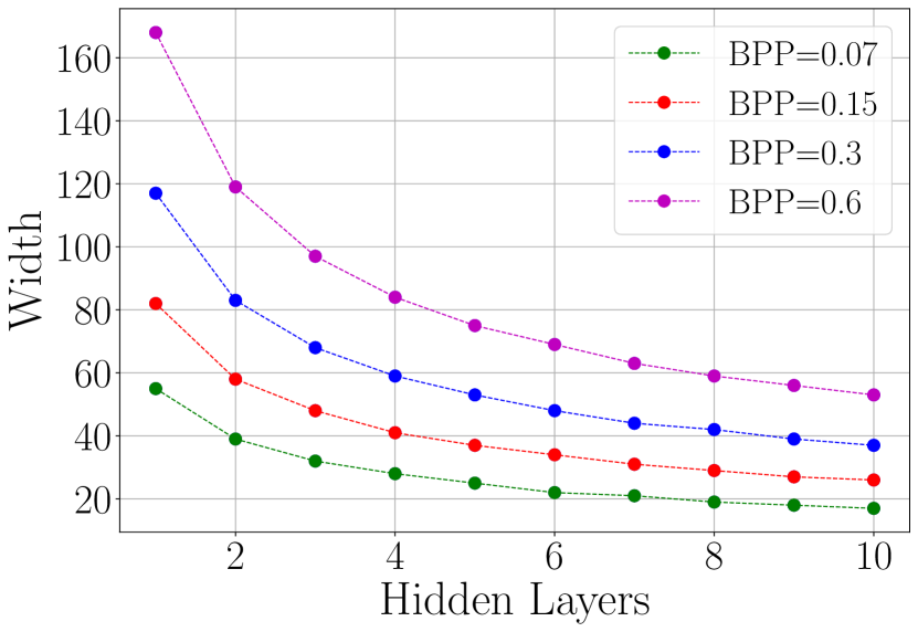
Figure 4: Left: COIN architectures show variability in outcome necessitating a costly Neural Architecture Search to achieve maximal performance as in [22]. Right: Architectures that satisfy a bits-per-pixel constraint for COIN (Kodak index 2) using 16-bit quantization. Extending the quantization range (to apply quantization-aware training, for example) multiplicatively increases the feasible architecture set.

3 Method

3.1 Training Configurations and Metrics

We test the performance of D’OH on two implicit neural compression tasks: image regression and occupancy field representation. We choose as a target network of 9 hidden layers and width 40, corresponding to the 0.6 BPP model for KODAK in [22]. We test latent code dimensions calculated to represent approximately 100%, 60%, and 30% of the parameters of the target MLP model as calculated without positional encoding. Note that the number of parameters increases for MLP models with positional encoding, but not with D’OH (see: Section 5.0.1 for discussion). For baselines we train MLP models using the MLP configurations in COIN corresponding to 0.07, 0.15, 0.3 BPP [22]. Table 1 outlines the full set of configurations used for training. We experiment both with and without positional encoding (10 Fourier frequencies [57]). Following training we apply post-training quantization to model weights at the best performing epoch and calculate the perceptual metrics at each quantization level. Compression metrics are reported using the estimated memory footprint (parameters $\times$ bits-per-parameter) and the bits-per-pixel (memory/pixels). We find this to be a close proxy to the performance of an entropy compressor (BZIP2 [72]), with some variation due to file overhead. See Supplementary Materials 2.0.1 for technical details of the applied post-training quantization strategy and compression.

Table 1: Training configurations for image and occupancy field experiments.

Dataset	KODAK	Thai Statue
Dimensions	$768\times 512$	$512\times 512\times 512$
Hardware	NVIDIA A100	NVIDIA A100
Optimizer	Adam $\beta=(0.99,0.999)$	Adam $\beta=(0.99,0.999)$
Scheduler (Exponential)	$\gamma=0.999$	$\gamma=0.999$
Epochs	2000	250
Batch Size	1024	20000
Loss	Mean Square Error	Mean Square Error
Perceptual Metrics	PSNR, SSIM[83], LPIPS[93]	IOU
Compression Metrics	Bits-Per-Pixel (BPP)	Memory (kB)
Target MLPs: width/hidden	20/4, 30/4, 28/9, 40/9	20/4, 30/4, 28/9, 40/9
Positional Encoding	10 frequencies	10 frequencies
Activation	Sine ($\omega=30$)	Sine ($\omega=30$)
Learning Rates (MLP/DOH)	$2{e-4}$,$1e{-6}$	$1{e-4}$, $1{e-6}$
Quantization levels	[4, 5, 6, 8, 16]	[4, 5, 6, 8, 16]

4 Results

4.0.1 Image Compression - KODAK

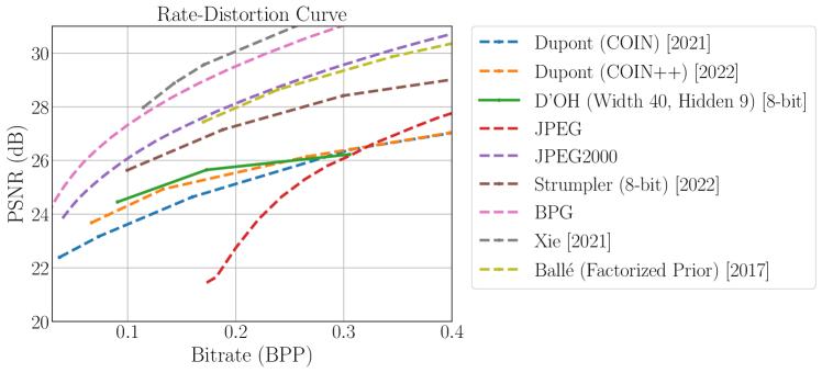
Figure 5: Rate-Distortion on Kodak showing additional benchmarks. Our method outperforms signal agnostic codecs trained without external datasets (COIN), our method lags both advanced signal specific codecs (JPEG2000 and BPG [11]), and those that employ auto-encoding [8], invertible encoding networks [88], and meta-learned initializations [76]. We suspect that the gap with [76] is due to the use of quantization aware training (QAT). As mentioned in Section 2.5.2, we avoid QAT as a primary motivation for our method is to reduce the need for architecture search, including different quantization levels (the post-training quantization strategy we employ avoids this).

Image regression is a $\mathbb{R}^{2}:\mathbb{R}^{3}$ coordinate function used to implicitly represent 2D images by predicting RGB values at sampled coordinates. We conduct image compression experiments on the Kodak dataset [2]. The Kodak dataset consists of natural images with dimensions $(768,512)$ and is a common test for implicit neural image compression (e.g. [22, 23, 76, 19]. We test across the 24 image Kodak dataset and report rate-distortion performance for the 100%, 60%, and 30% latent code dimensions, using 8-bit post-training quantization. Figure 5 shows the performance of D’OH relative to other algorithms, with comparison algorithms as reported by CompressAI [9]. D’OH shows improved performance relative to JPEG, COIN, and COIN++. We select these three benchmarks to highlight as a signal specific code (JPEG), data-agnostic and data-less codec (COIN) [22], and a meta-learned data-agnostic codec (COIN++) [23]; however, our most direct point of comparison is the original COIN as it relies on no external data or signal specific information. In the Supplementary Materials 3.1 we provide additional benchmarks showing performance relative to general leading compression methods, including those incorporating meta-learned quantization aware training [76], auto-encoders [7], and advanced image codecs [11].

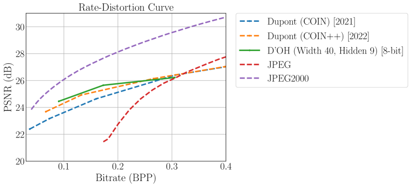
Figure 5: Rate-Distortion curve on the KODAK dataset. D’OH approximates a single target architecture (Width 40, Hidden 9) with fixed [post-training quantization (8-bits). The rate distortion curve is generated by varying the latent code dimension. The D’OH model exceeds the performance of JPEG, COIN, and COIN++.

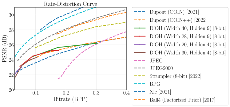
Figure 6: Ablation running D’OH with alternative COIN target networks. We note that D’OH is able to achieve a rate-distortion improvement on each of these architectures. The resulting model overlay shows an indicative Pareto frontier of the method.

Figure 6 shows an ablation showing the impacts of quantization and varying latent dimension. For completeness we include a D’OH model with 100% of the higher parameter count of including positional encoding. We can contrast here two methods for reducing the rate of a fixed MLP: weight quantization and varying the generating latent dimension. Quantization of the target MLP has a sharp drop off in performance below 16-bit precision. Varying the latent code provides a smoother way to interpolate performance between different bit-rates.

Qualitative results are shown in Figure 7. As COIN is fixed at 16-bits [22], we use an additional MLP benchmark to show direct comparison to D’OH at 8-bit quantization. We can note that D’OH greatly outperforms the 8-bit MLP models, potentially due to reduced quantization error when using a single latent code. This is consistent with the ablation in Figure 6. When compared to COIN (16-bit), which uses different architectures to vary bit-rate, D’OH out-performs at all comparable bit-rates while using the same target architecture. Note that in this experiment we use positional encoding for the D’OH model (which uses no additional parameters), and no positional encoding for the MLP models. In the Supplementary Experiments 3.1 we show reduced rate-distortion performance for very low-rate MLP models with positional encoding, due to increased parameters. We discuss this further in Section 5.0.1.

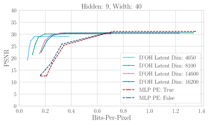
Figure 6: Comparison of base model (9, 40) and D’OH with varied latent dimension (evaluated on Kodak index 12). Rate-distortion curves generated by varying quantization levels. The D’OH model is more robust to quantization, with little loss of performance until around 8-bit. Varying the D’OH latent dimension is able to achieve smoother rate-distortion performance for a target MLP architecture than through quantization.

4.0.2 Occupancy Field Experiments

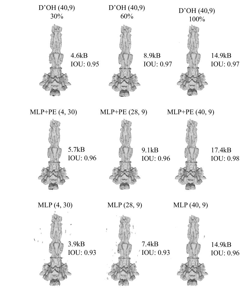
Figure 8: Expanded Qualitative Results from Figure 7, showing the effect of positional encoding on 8-bit MLPs. Positional encoding is critical for the reconstruction quality of MLPs, but at the cost of increased memory. By using a latent code independent of the input dimension, D’OH receives positional encoding without an increase in parameters. Memory sizes shown following BZIP2.

A binary occupancy Field is a $\mathbb{R}^{3}:\mathbb{R}^{1}$ coordinate function used to implicitly represent 3D shapes through point occupancy, with the output representing a prediction of voxel occupancy [56]. We test the ability of DOH to represent occupancy fields by exploring the implementation provided by [65] using the Thai Statue instance [1]. As noted by this paper, the occupancy training set is constructed by sampling voxels within a $512\times 512\times 512$ grid. As in the image experiments, we use a target network of (40, 9), and approximate this with smaller latent codes. We report performance using intersection over union (IOU). Qualitative results and are generated by applying marching cubes across a thresholded set of sampled coordinates [51], and are shown in Figure 7. In contrast to the image regression experiments, where a direct rate-distortion improvement is observed for the D’OH model when compared to low-rate MLPs, we find that the performance is more similar - this is due to positional encoding improving the rate distortion performance of the MLP models (see: Figure 8. In the Supplementary Materials 3.1 we provide additional qualitative results on occupancy field showing the effect of positional encoding for MLPs and D’OH. While a rate-distortion improvement is not observed for occupancy, we note that D’OH is able to smoothly vary the bit-rate of the target model without the use of alternative network structures.

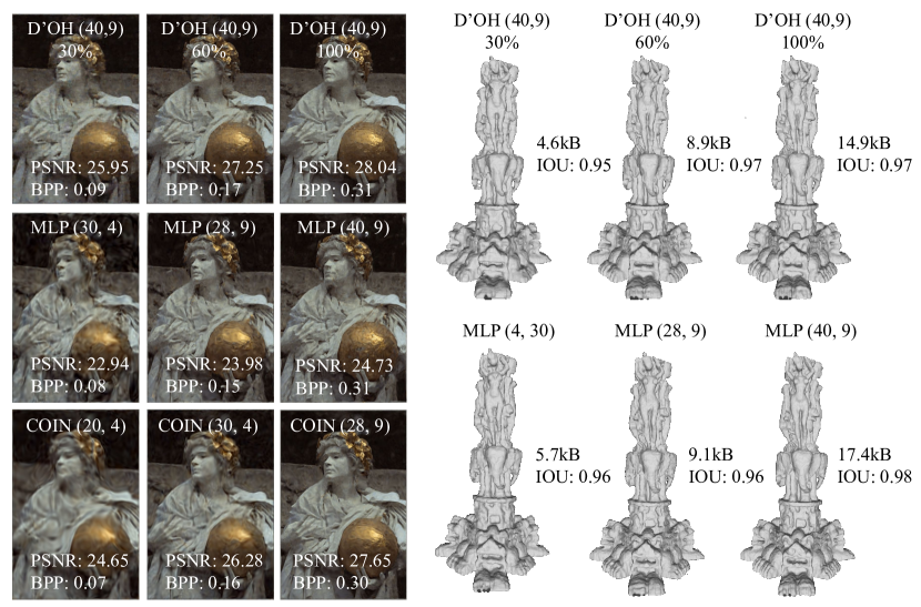
Figure 7: Qualitative image and occupancy field results. Left: Kodak. The top row corresponds to D’OH (8-bit quantization) with a target model (40 width, 9 hidden layers) with varied latent dimension. The second and third rows are MLPs (8-bit and 16-bit [COIN]) to match approximate bit-rates. Right: Occupancy field. The target model matches the bit-rate of a MLP (40 width, 9 hidden) without positional encoding. Note that D’OH models can receive positional encoding without an increase in parameters.

5 Discussion

In the previous section we demonstrated that a decoder-only hypernetwork is able to compactly represent a signal using a small latent code and demonstrate its potential for signal agnostic compression by quantizing in a manner similar to COIN [22]. Here we outline two interesting aspects of the model that occur from using a latent code and random projections to approximate a target network.

5.0.1 Positional Encoding

The number of parameters used in the decoder-only hypernetwork model is independent of the dimensions of the target network. An interesting consequence of this is that while including a positional encoding component to a multi-layer perceptron increases the number of parameters (due to the increased input dimension), this is not true for D’OH. As a result the D’OH model is able to use positional encoding "for free". As Figure 8 shows, for very low small networks the change in parameters induced by positional encoding can be significant. We find in Figure 6 that the increase is sufficient to lead to reduced rate-distortion performance for small MLPs on image regression with positional encoding. This contrasts [76], who find benefits of positional encoding within image experiments when combined with quantization aware training. In contrast, for the occupancy experiments we find that both the MLP and D’OH models noticeably improve in rate-distortion when applying positional encoding.

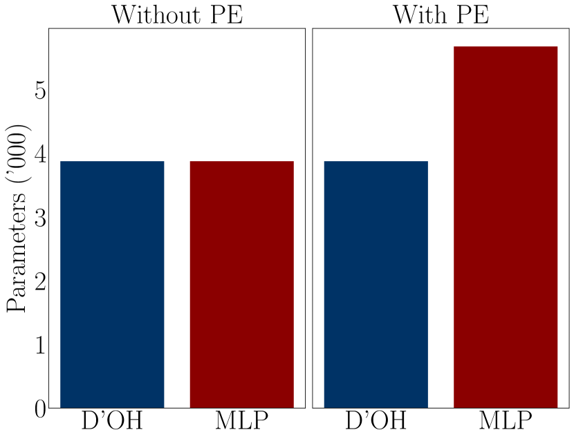
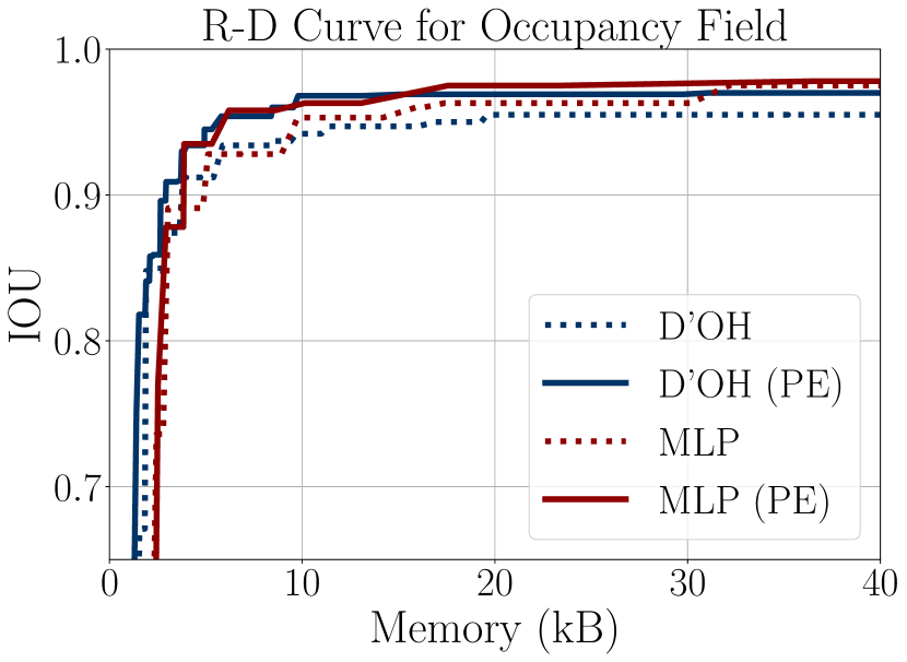
Figure 8: (a) Positional Encoding increases the parameter count of MLPs but not DOH. Comparison on target architecture of (4,28): using a 10 frequency positional encoding increases the number of MLP parameters by 46%. (b) Rate-Distortion on occupancy fields shows that both MLPs and DOH benefit from the use of positional encoding. Rate distortion shown for all tested quantization levels, latent codes, and architectures.

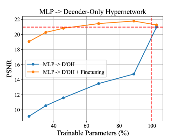
Figure 9: The blue line represents the evaluated performance immediately following inverting for the latent code. The orange line after fine-tuning for 100 epochs. The dotted red-line shows the target MLP parameters and performance. Performance exceeds or matches the pre-trained MLP on DIV2K with around half of the trainable parameters.

5.0.2 Direct MLP to Latent Code Projection

Algorithm 1 Pre-Trained MLP-to-DOH Projection

1:Input: Pretrained MLP weights $\{W_{l}\}_{l=1}^{L}$

2:Output: Decoder-only hypernetwork parameters

3:Extract $W$ as the stack of vectorized MLP weights $\text{vec}(W_{l})$ for all layers $l$

4:Initialize $B$ as a stack of arbitrary random $B_{l}$ for all layers $l$ as per Eq. (3)

5:Compute $z\approx B^{\dagger}W$

6:for each bias term in the MLP do

7:     Copy the per-layer MLP bias to DOH

8:end for

9:Fine-tune DOH for $N$ epochs

10:

11:Optional:

12:Quantize the parameters of the DOH

13:Compress the DOH state dictionary ($z$, biases, and integer seed) using BZIP2 or a similar entropy encoder.

By varying the latent code dimension of D’OH it is possible to achieve improved rate-distortion performance relative to a target architecture. While we have shown that this can achieve improved rate-distortion performance, we note that it suffers from a limitation common to COIN - needing to be trained from scratch for each tested latent code dimension [22]. However, the linear structure we have investigated raises the question of whether we can direct distill the parameters of a trained neural representation into a least-squares optimal latent code. Algorithm 1 outlines this approach. We take a pre-trained MLP and attempt to directly invert the system for the latent code $z$. The least-squares optimal projection is obtained by $z\approx B^{\dagger}W$ where $W$ is the stack of vectorized MLP weights $\text{vec}(W_{l})$, $\dagger$ denotes the Moore-Penrose pseudoinverse [75], and $B$ is a stack of arbitrary $(B_{l})$ initialised from Equation (3). For small coordinate networks and latent code dimensions this is computationally feasible and can be solved in less than a minute. The biases are copied to the hypernetwork directly. Figure 9 shows the results of this procedure applied to a 3 hidden layer, 32 width MLP pre-trained on a $512\times 512$ image from the DIV2K dataset [4]; before projecting to hypernetworks at lower dimension. We find that while direct inversion is not able to achieve satisfactory results immediately following projection, that fine-tuning the hypernetwork for 100 epochs achieves equivalent or improved performance to the target MLP with less than 50% of the original parameters. In effect, this suggests an efficient two-stage training method for decoder-only hypernetworks in which the first stage trains a target MLP and the second stage projects the MLP into a lower-dimension decoder-only hypernetwork which is a topic for future work.

6 Conclusions and Future Work

6.0.1 Conclusion

In conclusion we have provided a framework for direct optimization of a decoder-only hypernetwork for implicit neural representations. Contrasting prior work applying hypernetworks to implicit neural representations, our method does not require offline preconditioning on a target signal class and is instead able to be trained at runtime only the target data instance. As an example of this approach we have outlined a decode-only strategy to approximate a target architecture through a generating latent code and fixed random projection matrices. We have shown a number of surprising advantages to this approach, including: improved rate-distortion performance on image compression; smooth interpolation of bit-rate for target network architectures without the need for neural architecture search on low-rate structures or aggressive quantization. We note the improvement over quantization for reducing the rate of a fixed target architecture is especially pronounced. Hence, our method is potentially most applicable as a method to compress target implicit neural representations.

6.0.2 Future Work

While our model has been experimentally demonstrated on images and occupancy fields we believe that it may be applicable to other implicit neural signal types, such as point clouds, neural radiance fields, sign-distance functions, and sound files [87]. Our strategy highlights the potential to exploit neural network redundancy for compression through the precommunication of arbitrary non-trained values to further compress a transmitted learned signal code. We consider that our approach may be complementary to recent techniques used in the compression of implicit neural representations, such as quantization aware training [76], non-uniform adaptive quantization [33], and sparsification [89].

Supplementary Materials
D’OH: Decoder-Only random Hypernetworks for Implicit Neural Representations

1 Initialization

In Section 2.5.1 we noted that we need to apply a modified initialization scheme under the random matrix hypernetwork structure we examine. Under most intiialization schemes (e.g. He [37], Xavier [31], and SIREN [74]), initialization is conducted separately for each layer - a property we want to preserve in the target network. However as we will use the same latent parameter vector to generate each layer we will instead need to account for this by changing the per-layer random matrices to match the desired initialization of the target network.

1.1 Derivation

Assume the entries of $z$ are drawn independently and identically distributed from a distribution of variance $\text{Var}(z)$, and that the weights of the $l^{th}$ layer of the target network are to have variance $\text{Var}(W_{l})$. We seek a formula for the variance $\text{Var}(B_{l})$ of the distribution from which to independently and identically draw the entries of the random matrix $B_{l}$ such that the entries of $B_{l}z$ have variance $\text{Var}(W_{l})$. We assume that all entries for both $z$ and $B_{l}$ are drawn independently of one another, and with zero mean. From Equation 2, we have:

$$\bar{W}_{l}=B_{l}z.$$ (1)

Recall that $n$ denotes the dimension of $z$, and use superscripts to denote vector and matrix indices. Then the above equation can be written entry-wise as:

$$\text{Var}(\bar{W}_{l}^{i})=\text{Var}(\sum\limits_{j=1}^{n}B_{l}^{ij}z^{j})$$ (2)

Since the entries of $B_{l}$ and $z$ are all independent, we therefore have:

$$\text{Var}(\bar{W}_{l}^{i})=\sum\limits_{j=1}^{n}\text{Var}(B_{l}^{ij}z^{j}).$$ (3)

Again using independence of the entries of $B_{l}$ and $z$, we have:

$$\begin{split}\text{Var}(\bar{W}_{l}^{i})&=\sum\limits_{j=1}^{n}\text{Var}(B_{l}^{ij})\text{Var}(z^{j})\\ &+\text{Var}(B_{l}^{ij})\mathbb{E}(z^{j})^{2}+\mathbb{E}(B_{l}^{ij})^{2}\text{Var}(z^{j}),\end{split}$$ (4)

which simplifies to:

$$\text{Var}(\bar{W}_{l}^{i})=\sum\limits_{j=1}^{n}\text{Var}(B_{l}^{ij})\text{Var}(z^{j})$$ (5)

by our zero-mean assumption on the entries of $B_{l}$ and $z$. Invoking our identically distributed assumption finally yields:

$$\text{Var}(\bar{W}_{l})=n\text{Var}(B_{l})\text{Var}(z),$$ (6)

so that:

$$\text{Var}(B_{l})=\frac{\text{Var}(\bar{W}_{l})}{n\text{Var}(z)}.$$ (7)

We will use this formula to find bounds on a uniform distribution for $B_{l}$ in order to achieve the variance $\text{Var}(W_{l})$ of the weights considered in [74]. To initialize $B_{l}$ using a uniform distribution centred at 0, we must determine its bounds $\pm a$. Taking the variance of a uniform distribution, we have $\text{Var}(B_{l})=\frac{1}{12}(2a)^{2}=\frac{a^{2}}{3}$. Substituting into Equation (7), we have:

$$\frac{a^{2}}{3}=\frac{\text{Var}(\bar{W_{l}})}{n\text{Var}(z)},$$ (8)

so that

$$a=\pm\sqrt{\frac{3\text{Var}(\bar{W_{l}})}{n\text{Var}(z)}}.$$ (9)

1.2 SIREN Equivalent Initialization

We can apply Equation (9) to derive an example SIREN initialization [74].

Input Layer: Assume $z$ is initialized using $U\sim(\pm\frac{1}{n})$ and $\bar{W}_{0}$ by $U\sim(\pm\frac{1}{fan_{in}})$ where $fan_{in}$ represents the input dimension of the target network:

$$\text{Var}(\bar{W_{0}})=\frac{1}{12}(\frac{2}{fan_{in}})^{2}=\frac{1}{3fan_{in}^{2}}$$ (10)

$$\text{Var}(z)=\frac{(2/n)^{2}}{12}=\frac{1}{3n^{2}}$$ (11)

$$\text{Var}(B_{0})=\frac{\text{Var}(\bar{W_{i}})}{n\text{Var}(z)}=\frac{1/(3fan_{in}^{2})}{n/(3n^{2})}=\frac{n}{fan_{in}^{2}}$$ (12)

$$a_{0}=\pm\sqrt{\frac{3n}{fan_{in}^{2}}}$$ (13)

Other Layers: $\bar{W_{i}}$ initialized using $U\sim(\pm\frac{1}{\omega\sqrt{h}})$, where $h$ refers to the number of hidden units, and $\omega$ the SIREN frequency.

$$\text{Var}(\bar{W_{i}})=\frac{1}{12}(\frac{2}{\omega\sqrt{h}})^{2}=\frac{1}{3\omega^{2}h}$$ (14)

$$\text{Var}(B_{i})=\frac{\text{Var}(\bar{W_{i}})}{n\text{Var}(z)}=\frac{1/(3\omega^{2}h)}{n/(3n^{2})}=\frac{n}{\omega^{2}h}$$ (15)

$$a_{i}=\pm\sqrt{\frac{3n}{\omega^{2}h}}$$ (16)

1.2.1 Numerical Comparison

We initialize target networks with using Equations (13) and (16) for a range of input and hidden layer dimensions. The D’OH initialization correctly matches the target SIREN weight variances (Figure 1 ).

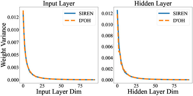
Figure 1: Numerical comparison of layer variances between SIREN and the weights generated by D’OH (latent dim: 2000 and $\omega=30$). Our initialization closely matches the initialization of SIREN [74].

2 Quantization, Compression, and Transmission

2.0.1 Quantization

We outline here the design decisions for our quantization approach. We employ post-training quantization in our pipeline. While quantization-aware training (QAT) [64] has been demonstrated to reduce quantization error in the context of implicit neural representations [76, 23, 19, 33], we note this has two key disadvantages: each quantization level needs to be trained separately, while post-training quantization can evaluate multiple quantization levels at the same time; and when quantization level is considered as part of the neural architecture search (see: Figure 4) this expands the search space of satisfying models considerably. In addition, we employ a layer-wise range-based integer quantization scheme between the min and maximum values for each weight and distribution [30]. We select an integer scheme to reduce the quantization symbol set [30, 29, 39]. We decided on a uniform quantization scheme rather than a non-linear quantizer such as k-means [36] due to the overhead of code-book storage, which for small networks can be substantial proportion of compressed memory [33]. In contrast, we represent each tensor with just three per-tensor components (integer tensor, minimum value, maximum value). Similar range-based integer quantization schemes are commonly described [30, 39, 45], and the method we use is only a subtle variation avoiding the explicit use of a zero point.

2.0.2 Compression and Transmission

In a typical compressed implicit neural network the entire trained and compressed network weights need to be transferred between parties. This is done by first quantizing the weights followed by a lossless entropy compressor, such as BZIP2 [72] or arithmetic coding [76]. Our method generates a target network by a low-dimensional linear code and fixed per-layer random matrices. As random matrices can be reconstructed by the transfer of an integer seed, we only quantize and compress the linear code. The recently proposed VeRA incorporates a similar integer seed transmission protocol for random matrices to improve the parameter efficiency of Low-Rank Adaptive Models [44].

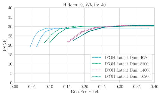
Figure 2: Comparison of bits-per-pixel (BPP) for estimated memory footprint (parameters $\times$ bits-per-weight) [dotted] and memory after applying BZIP2 [solid] to a Python pickle of the quantized model. Rate-distortions generated by varying quantization level. The estimated is a close proxy to an actual entropy coder, but shows some discrepancy at low-rate and low-quantization levels where file overhead represent a larger proportion of code size. In this paper we typically report for the estimated memory footprint for both D’OH and MLPs, which can be seen as a theoretical limit for performance.

3 Additional Results

3.1 Ablations

Figure 3: Comparison for four target D’OH architectures (4,20), (4,30), (9,28), (9,40) with rate-distortion generated by varying quantization levels at [4, 5, 6, 8, 16, 32] bits per parameter. Top: Kodak (index 12), bottom: Occupancy Field. The D’OH model is able to achieve improved rate distortion to each of the target architectures by varying latent dimension. For images D’OH shows less severe quantization error relative to the MLPs. We note that the MLP models show worse rate-distortion performance with positional encoding for images, but occupancy fields show an improvement. For images the impact is most apparent for low-rate MLPs. This is likely due to a higher proportional increase in parameters for low-rate architectures relative to larger models.

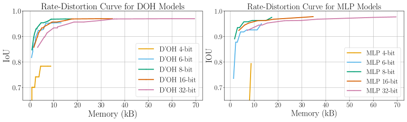
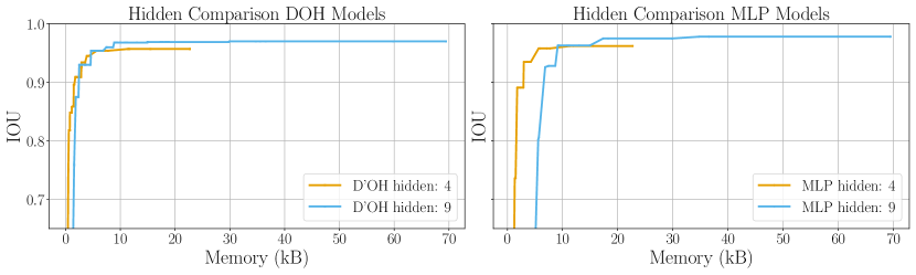
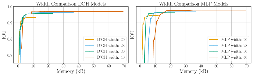
Figure 4: Occupancy field ablation showing the relative changes in performance with different architecture components (quantization level, hidden, and width) for D’OH and MLP models). Rate-distortions generated by varying the uncompared components. We observe that changing the target architecture (width, hidden) does not greatly affect the D’OH memory profile as the latent dimension remains fixed, with only the bias increasing total parameter count. The D’OH model is relatively more robust to higher levels of quantization (e.g. 6-bit) compared to the MLP. Higher performance is observed for the deeper D’OH models, indicating that despite projecting a linear code the model is able to derive a performance benefit from the deeper target architecture.

3.2 Further Benchmarks

3.3 Additional Qualitative Results - Kodak

Figure 7: Additional qualitative results on Kodak showing the comparison between 8-bit D’OH, 8-bit MLP, and COIN (a MLP quantized to 16-bits). Note that smaller COIN architectures are required to match the comparison bit-rates. D’OH is more robust to quantization than the MLP models. D’OH uses positional encoding, while the MLP models do not (see: Figure 3 - PE is detrimental to low-rate MLP performance).

3.4 Additional Qualitative Results - Occupancy Field

References

- [1] The Stanford 3D Scanning Repository. http://graphics.stanford.edu/data/3Dscanrep/
- [2] True Color Kodak Images (1991)
- [3] Aghajanyan, A., Gupta, S., Zettlemoyer, L.: Intrinsic Dimensionality Explains the Effectiveness of Language Model Fine-Tuning. In: Proceedings of the 59th Annual Meeting of the Association for Computational Linguistics and the 11th International Joint Conference on Natural Language Processing (Volume 1: Long Papers). pp. 7319–7328. Association for Computational Linguistics, Online (Aug 2021). https://doi.org/10/gmf9pk
- [4] Agustsson, E., Timofte, R.: NTIRE 2017 Challenge on Single Image Super-Resolution: Dataset and Study. In: 2017 IEEE Conference on Computer Vision and Pattern Recognition Workshops (CVPRW). pp. 1122–1131. IEEE, Honolulu, HI, USA (Jul 2017). https://doi.org/10/ggk6gn
- [5] Alaluf, Y., Tov, O., Mokady, R., Gal, R., Bermano, A.: HyperStyle: StyleGAN Inversion with HyperNetworks for Real Image Editing. In: 2022 IEEE/CVF Conference on Computer Vision and Pattern Recognition (CVPR). pp. 18490–18500. IEEE, New Orleans, LA, USA (Jun 2022). https://doi.org/10/gtnwn5
- [6] Arora, S., Ge, R., Neyshabur, B., Zhang, Y.: Stronger Generalization Bounds for Deep Nets via a Compression Approach. In: Proceedings of the 35th International Conference on Machine Learning. pp. 254–263. PMLR (Jul 2018)
- [7] Ballé, J., Chou, P.A., Minnen, D., Singh, S., Johnston, N., Agustsson, E., Hwang, S.J., Toderici, G.: Nonlinear Transform Coding (Oct 2020). https://doi.org/10.48550/arXiv.2007.03034
- [8] Ballé, J., Laparra, V., Simoncelli, E.P.: End-to-end Optimized Image Compression (Mar 2017). https://doi.org/10.48550/arXiv.1611.01704
- [9] Bégaint, J., Racapé, F., Feltman, S., Pushparaja, A.: CompressAI: A PyTorch library and evaluation platform for end-to-end compression research. arXiv:2011.03029 (Nov 2020)
- [10] Belbute-Peres, F.d.A., Chen, Y.f., Sha, F.: HyperPINN: Learning parameterized differential equations with physics-informed hypernetworks. arXiv.org (Oct 2021)
- [11] Bellard, F.: BPG Image format. https://bellard.org/bpg/
- [12] Bingham, E., Mannila, H.: Random projection in dimensionality reduction: Applications to image and text data. In: Proceedings of the Seventh ACM SIGKDD International Conference on Knowledge Discovery and Data Mining. pp. 245–250. KDD ’01, Association for Computing Machinery, New York, NY, USA (2001). https://doi.org/10/dj7jn6
- [13] Chang, O., Flokas, L., Lipson, H.: Principled Weight Initialization for Hypernetworks (2020)
- [14] Chauhan, V.K., Zhou, J., Lu, P., Molaei, S., Clifton, D.A.: A Brief Review of Hypernetworks in Deep Learning. arXiv.org (Jun 2023)
- [15] Chen, H.: An Efficient Neural Representation for Videos. Ph.D. thesis (2023)
- [16] Chen, H., He, B., Wang, H., Ren, Y., Lim, S.N., Shrivastava, A.: NeRV: Neural Representations for Videos. In: Advances in Neural Information Processing Systems. vol. 34, pp. 21557–21568. Curran Associates, Inc. (2021)
- [17] Chen, Y., Wang, X.: Transformers as Meta-Learners for Implicit Neural Representations. arXiv.org (Aug 2022)
- [18] Chiarlo, F.M.: Implicit Neural Representations for Image Compression (Jul 2021)
- [19] Damodaran, B.B., Balcilar, M., Galpin, F., Hellier, P.: RQAT-INR: Improved Implicit Neural Image Compression (Mar 2023)
- [20] Dasgupta, S., Gupta, A.: An elementary proof of a theorem of Johnson and Lindenstrauss. Random Structures & Algorithms 22(1), 60–65 (2003). https://doi.org/10/cb9srh
- [21] Denil, M., Shakibi, B., Dinh, L., Ranzato, M.A., de Freitas, N.: Predicting Parameters in Deep Learning. In: Advances in Neural Information Processing Systems. vol. 26. Curran Associates, Inc. (2013)
- [22] Dupont, E., Goliński, A., Alizadeh, M., Teh, Y.W., Doucet, A.: COIN: COmpression with Implicit Neural representations. arXiv:2103.03123 (2021)
- [23] Dupont, E., Loya, H., Alizadeh, M., Goliński, A., Teh, Y.W., Doucet, A.: COIN++: Neural Compression Across Modalities (2022). https://doi.org/10.48550/ARXIV.2201.12904
- [24] Elsken, T., Metzen, J.H., Hutter, F.: Neural Architecture Search: A Survey. Journal of Machine Learning Research 20(55), 1–21 (2019)
- [25] Finn, C., Abbeel, P., Levine, S.: Model-Agnostic Meta-Learning for Fast Adaptation of Deep Networks. In: Proceedings of the 34th International Conference on Machine Learning. pp. 1126–1135. PMLR (Jul 2017)
- [26] Galanti, T., Wolf, L.: On the Modularity of Hypernetworks. In: Advances in Neural Information Processing Systems. vol. 33, pp. 10409–10419. Curran Associates, Inc. (2020)
- [27] Gao, S., Huang, F., Huang, H.: Model Compression via Hyper-Structure Network (Mar 2021)
- [28] Garnelo, M., Rosenbaum, D., Maddison, C.J., Ramalho, T., Saxton, D., Shanahan, M., Teh, Y.W., Rezende, D.J., Eslami, S.M.A.: Conditional Neural Processes (Jul 2018)
- [29] Gersho, A., Gray, R.: Vector Quantization and Signal Compression. The Kluwer International Series In Engineering And Computer Science, Kluwer International Publishers (1992)
- [30] Gholami, A., Kim, S., Dong, Z., Yao, Z., Mahoney, M.W., Keutzer, K.: A Survey of Quantization Methods for Efficient Neural Network Inference. In: Low-Power Computer Vision. Chapman and Hall/CRC (2022)
- [31] Glorot, X., Bengio, Y.: Understanding the difficulty of training deep feedforward neural networks. In: Proceedings of the Thirteenth International Conference on Artificial Intelligence and Statistics. pp. 249–256. JMLR Workshop and Conference Proceedings (Mar 2010)
- [32] Goodfellow, I., Bengio, Y., Courville, A.: Deep Learning. MIT Press (2016)
- [33] Gordon, C., Chng, S.F., MacDonald, L., Lucey, S.: On Quantizing Implicit Neural Representations. In: Proceedings of the IEEE/CVF Winter Conference on Applications of Computer Vision (WACV). pp. 341–350 (Jan 2023)
- [34] Ha, D., Dai, A., Le, Q.V.: HyperNetworks (Dec 2016). https://doi.org/10.48550/arXiv.1609.09106
- [35] Halko, N., Martinsson, P.G., Tropp, J.A.: Finding Structure with Randomness: Probabilistic Algorithms for Constructing Approximate Matrix Decompositions. SIAM Review 53(2), 217–288 (Jan 2011). https://doi.org/10/cdgnkv
- [36] Han, S., Mao, H., Dally, W.J.: Deep Compression: Compressing Deep Neural Networks with Pruning, Trained Quantization and Huffman Coding. International Conference on Learning. Representations (ICLR) (Feb 2016). https://doi.org/10.48550/arXiv.1510.00149
- [37] He, K., Zhang, X., Ren, S., Sun, J.: Deep Residual Learning for Image Recognition. In: 2016 IEEE Conference on Computer Vision and Pattern Recognition (CVPR). pp. 770–778 (Jun 2016). https://doi.org/10/gdcfkn
- [38] Hinton, G., Vinyals, O., Dean, J.: Distilling the Knowledge in a Neural Network (Mar 2015). https://doi.org/10.48550/arXiv.1503.02531
- [39] Jacob, B., Kligys, S., Chen, B., Zhu, M., Tang, M., Howard, A., Adam, H., Kalenichenko, D.: Quantization and Training of Neural Networks for Efficient Integer-Arithmetic-Only Inference. arXiv:1712.05877 [cs, stat] (Dec 2017)
- [40] Johnson, W.B., Lindenstrauss, J.: Extensions of Lipschitz mappings into Hilbert space. Contemporary mathematics 26, 189–206 (1984). https://doi.org/10/fzff89
- [41] Karimi Mahabadi, R., Ruder, S., Dehghani, M., Henderson, J.: Parameter-efficient Multi-task Fine-tuning for Transformers via Shared Hypernetworks. In: Proceedings of the 59th Annual Meeting of the Association for Computational Linguistics and the 11th International Joint Conference on Natural Language Processing (Volume 1: Long Papers). pp. 565–576. Association for Computational Linguistics, Online (Aug 2021). https://doi.org/10/gm6jbj
- [42] Kim, H., Bauer, M., Theis, L., Schwarz, J.R., Dupont, E.: C3: High-performance and low-complexity neural compression from a single image or video. In: Proceedings of the IEEE/CVF Conference on Computer Vision and Pattern Recognition (CVPR) (2024)
- [43] Klocek, S., Maziarka, Ł., Wołczyk, M., Tabor, J., Nowak, J., Śmieja, M.: Hypernetwork Functional Image Representation. In: Artificial Neural Networks and Machine Learning – ICANN 2019: Workshop and Special Sessions. pp. 496–510. Lecture Notes in Computer Science, Springer International Publishing, Cham (2019). https://doi.org/10/gkqs5b
- [44] Kopiczko, D.J., Blankevoort, T., Asano, Y.M.: VeRA: Vector-based Random Matrix Adaptation. In: International Conference on Learning Representations (2024)
- [45] Krishnamoorthi, R.: Quantizing deep convolutional networks for efficient inference: A whitepaper (Jun 2018). https://doi.org/10.48550/arXiv.1806.08342
- [46] Ladune, T., Philippe, P., Henry, F., Clare, G., Leguay, T.: COOL-CHIC: Coordinate-based Low Complexity Hierarchical Image Codec. In: 2023 IEEE/CVF International Conference on Computer Vision (ICCV). pp. 13469–13476. Los Alamitos, CA, USA (Oct 2023). https://doi.org/10/gtnwnj
- [47] Lee, J., Tack, J., Lee, N., Shin, J.: Meta-Learning Sparse Implicit Neural Representations. In: Advances in Neural Information Processing Systems. vol. 34, pp. 11769–11780. Curran Associates, Inc. (2021)
- [48] Li, X., Kaesemodel Pontes, J., Lucey, S.: Neural Scene Flow Prior. In: Advances in Neural Information Processing Systems. vol. 34, pp. 7838–7851. Curran Associates, Inc. (2021)
- [49] Littwin, E., Galanti, T., Wolf, L., Yang, G.: On Infinite-Width Hypernetworks. In: Advances in Neural Information Processing Systems. vol. 33, pp. 13226–13237. Curran Associates, Inc. (2020)
- [50] Liu, Z., Luo, P., Wang, X., Tang, X.: Deep Learning Face Attributes in the Wild (Sep 2015). https://doi.org/10.48550/arXiv.1411.7766
- [51] Lorensen, W.E., Cline, H.E.: Marching cubes: A high resolution 3D surface construction algorithm. In: Proceedings of the 14th Annual Conference on Computer Graphics and Interactive Techniques. pp. 163–169. SIGGRAPH ’87, Association for Computing Machinery, New York, NY, USA (1987). https://doi.org/10.1145/37401.37422
- [52] Lu, Y., Jiang, K., Levine, J.A., Berger, M.: Compressive Neural Representations of Volumetric Scalar Fields (Apr 2021). https://doi.org/10.48550/arXiv.2104.04523
- [53] Majumdar, R., Jadhav, V., Deodhar, A., Karande, S., Vig, L., Runkana, V.: HyperLoRA for PDEs. https://arxiv.org/abs/2308.09290v1 (Aug 2023)
- [54] Martinez, J., Shewakramani, J., Wei Liu, T., Andrei Barsan, I., Zeng, W., Urtasun, R.: Permute, Quantize, and Fine-tune: Efficient Compression of Neural Networks. In: 2021 IEEE/CVF Conference on Computer Vision and Pattern Recognition (CVPR). pp. 15694–15703. IEEE, Nashville, TN, USA (Jun 2021). https://doi.org/10/grkghq
- [55] McDonnell, M.D., Gong, D., Parvaneh, A., Abbasnejad, E., van den Hengel, A.: RanPAC: Random Projections and Pre-trained Models for Continual Learning. In: Advances in Neural Information Processing Systems. vol. 36, pp. 12022–12053. Curran Associates, Inc. (2023)
- [56] Mescheder, L., Oechsle, M., Niemeyer, M., Nowozin, S., Geiger, A.: Occupancy Networks: Learning 3D Reconstruction in Function Space. In: Proceedings of the IEEE/CVF Conference on Computer Vision and Pattern Recognition (CVPR) (Jun 2019)
- [57] Mildenhall, B., Srinivasan, P.P., Tancik, M., Barron, J.T., Ramamoorthi, R., Ng, R.: NeRF: Representing scenes as neural radiance fields for view synthesis. In: Computer Vision – ECCV 2020. pp. 405–421. Springer International Publishing, Cham (2020)
- [58] Nguyen, P., Tran, T., Le, K., Gupta, S., Rana, S., Nguyen, D., Nguyen, T., Ryan, S., Venkatesh, S.: Fast Conditional Network Compression Using Bayesian HyperNetworks. arXiv.org (May 2022)
- [59] Nowlan, S.J., Hinton, G.E.: Simplifying Neural Networks by Soft Weight-Sharing. Neural Computation 4, 473–493 (1992). https://doi.org/10/dcv5q3
- [60] Park, J.J., Florence, P., Straub, J., Newcombe, R., Lovegrove, S.: DeepSDF: Learning Continuous Signed Distance Functions for Shape Representation. In: The IEEE Conference on Computer Vision and Pattern Recognition (CVPR) (Jun 2019)
- [61] Pham, T., Yang, Y., Mandt, S.: Autoencoding Implicit Neural Representations for Image Compression. In: ICML 2023 Workshop Neural Compression: From Information Theory to Applications (Jul 2023)
- [62] Pistilli, F., Valsesia, D., Fracastoro, G., Magli, E.: Signal Compression via Neural Implicit Representations. In: ICASSP 2022 - 2022 IEEE International Conference on Acoustics, Speech and Signal Processing (ICASSP). pp. 3733–3737 (May 2022). https://doi.org/10.1109/icassp43922.2022.9747208
- [63] Ramanujan, V., Wortsman, M., Kembhavi, A., Farhadi, A., Rastegari, M.: What’s Hidden in a Randomly Weighted Neural Network? (Mar 2020). https://doi.org/10.48550/arXiv.1911.13299
- [64] Rastegari, M., Ordonez, V., Redmon, J., Farhadi, A.: XNOR-Net: ImageNet Classification Using Binary Convolutional Neural Networks (2016). https://doi.org/10.48550/ARXIV.1603.05279
- [65] Saragadam, V., LeJeune, D., Tan, J., Balakrishnan, G., Veeraraghavan, A., Baraniuk, R.G.: WIRE: Wavelet Implicit Neural Representations (Jan 2023). https://doi.org/10.48550/arXiv.2301.05187
- [66] Savarese, P., Maire, M.: Learning Implicitly Recurrent CNNs Through Parameter Sharing (2019). https://doi.org/10.48550/ARXIV.1902.09701
- [67] Schwarz, J., Teh, Y.W.: Meta-Learning Sparse Compression Networks. Transactions on Machine Learning Research (2022)
- [68] Schwarz, J.R., Tack, J., Teh, Y.W., Lee, J., Shin, J.: Modality-Agnostic Variational Compression of Implicit Neural Representations. In: Proceedings of the 40th International Conference on Machine Learning. pp. 30342–30364. PMLR (Jul 2023)
- [69] Sen, B., Singh, G., Agarwal, A., Agaram, R., Krishna, K.M., Sridhar, S.: HyP-NeRF: Learning Improved NeRF Priors using a HyperNetwork. arXiv.org (Jun 2023)
- [70] Sendera, M., Przewięźlikowski, M., Karanowski, K., Zięba, M., Tabor, J., Spurek, P.: HyperShot: Few-Shot Learning by Kernel HyperNetworks. https://arxiv.org/abs/2203.11378v1 (Mar 2022)
- [71] Sendera, M., Przewiȩźlikowski, M., Miksa, J., Rajski, M., Karanowski, K., Ziȩba, M., Tabor, J., Spurek, P.: The general framework for few-shot learning by kernel HyperNetworks. Machine Vision and Applications 34(4), 53 (May 2023). https://doi.org/10/gtnwpx
- [72] Seward, J.: Bzip2 and Libbzip2 (1996)
- [73] Shi, J., Guillemot, C.: Distilled Low Rank Neural Radiance Field with Quantization for Light Field Compression (Jul 2022)
- [74] Sitzmann, V., Martel, J., Bergman, A., Lindell, D., Wetzstein, G.: Implicit Neural Representations with Periodic Activation Functions. In: Advances in Neural Information Processing Systems. vol. 33, pp. 7462–7473. Curran Associates, Inc. (2020)
- [75] Strang, G.: Linear Algebra and Learning from Data. Wellesley-Cambridge Press (2019)
- [76] Strümpler, Y., Postels, J., Yang, R., Gool, L.V., Tombari, F.: Implicit Neural Representations for Image Compression. In: Computer Vision – ECCV 2022. vol. 13686, pp. 74–91. Springer Nature Switzerland, Cham (2022). https://doi.org/10.1007/978-3-031-19809-0_5
- [77] Szatkowski, F., Piczak, K.J., Spurek, P., Tabor, J., Trzcinski, T.: HyperSound: Generating Implicit Neural Representations of Audio Signals with Hypernetworks. In: Sixth Workshop on Meta-Learning at the Conference on Neural Information Processing Systems (Nov 2022)
- [78] Takikawa, T., Evans, A., Tremblay, J., Müller, T., McGuire, M., Jacobson, A., Fidler, S.: Variable Bitrate Neural Fields (Jun 2022). https://doi.org/10.48550/arXiv.2206.07707
- [79] Takikawa, T., Müller, T., Nimier-David, M., Evans, A., Fidler, S., Jacobson, A., Keller, A.: Compact Neural Graphics Primitives with Learned Hash Probing. In: SIGGRAPH Asia 2023 Conference Papers. pp. 1–10. ACM, Sydney NSW Australia (Dec 2023). https://doi.org/10.1145/3610548.3618167
- [80] Tancik, M., Mildenhall, B., Wang, T., Schmidt, D., Srinivasan, P.P., Barron, J.T., Ng, R.: Learned Initializations for Optimizing Coordinate-Based Neural Representations. CVPR (Mar 2021). https://doi.org/10.1109/CVPR46437.2021.00287
- [81] Ullrich, K., Meeds, E., Welling, M.: Soft Weight-Sharing for Neural Network Compression. In: International Conference on Learning Representations (Nov 2016)
- [82] Wang, A.Q., Dalca, A.V., Sabuncu, M.R.: Computing Multiple Image Reconstructions with a Single Hypernetwork . https://doi.org/10/gtnwnm
- [83] Wang, Z., Bovik, A., Sheikh, H., Simoncelli, E.: Image quality assessment: From error visibility to structural similarity. IEEE Transactions on Image Processing 13(4), 600–612 (2004). https://doi.org/10/c7sr27
- [84] White, C., Safari, M., Sukthanker, R., Ru, B., Elsken, T., Zela, A., Dey, D., Hutter, F.: Neural Architecture Search: Insights from 1000 Papers (Jan 2023). https://doi.org/10.48550/arXiv.2301.08727
- [85] Wu, Q., Bauer, D., Chen, Y., Ma, K.L.: HyperINR: A Fast and Predictive Hypernetwork for Implicit Neural Representations via Knowledge Distillation (Apr 2023). https://doi.org/10.48550/arXiv.2304.04188
- [86] Xie, H., Li, J., Xue, H.: A survey of dimensionality reduction techniques based on random projection (May 2018)
- [87] Xie, Y., Takikawa, T., Saito, S., Litany, O., Yan, S., Khan, N., Tombari, F., Tompkin, J., Sitzmann, V., Sridhar, S.: Neural Fields in Visual Computing and Beyond (Apr 2022). https://doi.org/10.48550/arXiv.2111.11426
- [88] Xie, Y., Cheng, K.L., Chen, Q.: Enhanced Invertible Encoding for Learned Image Compression (Aug 2021)
- [89] Yüce, G., Ortiz-Jiménez, G., Besbinar, B., Frossard, P.: A Structured Dictionary Perspective on Implicit Neural Representations (Mar 2022). https://doi.org/10.48550/arXiv.2112.01917
- [90] Zhang, C., Ren, M., Urtasun, R.: Graph HyperNetworks for Neural Architecture Search. In: International Conference on Learning Representations (2019). arXiv (Dec 2020)
- [91] Zhang, G., Zhang, X., Tang, L.: Enhanced Quantified Local Implicit Neural Representation for Image Compression. IEEE Signal Processing Letters 30, 1742–1746 (2023). https://doi.org/10/gtnwnx
- [92] Zhang, K., Zhu, D., Min, X., Zhai, G.: Implicit Neural Representation Learning for Hyperspectral Image Super-Resolution. In: 2022 IEEE International Conference on Multimedia and Expo (ICME). pp. 1–6 (2022). https://doi.org/10/gtnwn7
- [93] Zhang, R., Isola, P., Efros, A.A., Shechtman, E., Wang, O.: The Unreasonable Effectiveness of Deep Features as a Perceptual Metric. In: CVPR (2018). https://doi.org/10/gfz33w