Correlation functions between singular values and eigenvalues

Abstract

Exploiting the explicit bijection between the density of singular values and the density of eigenvalues for bi-unitarily invariant complex random matrix ensembles of finite matrix size we aim at finding the induced probability measure on $j$ eigenvalues and $k$ singular values that we coin $j,k$-point correlation measure. We fully derive all $j,k$-point correlation measures in the simplest cases for one- and two-dimensional matrices. For $n>2$, we find a general formula for the $1,1$-point correlation measure. This formula reduces drastically when assuming the singular values are drawn from a polynomial ensemble, yielding an explicit formula in terms of the kernel corresponding to the singular value statistics. These expressions simplify even further when the singular values are drawn from a Pólya ensemble and extend known results between their eigenvalue and singular value statistics.

MSC Classification]60B20, 15B52, 43A90,42B10,42C05

1 Introduction

1.1 State of the art

For general complex square matrices, there exist various different decompositions. We are interested in two in particular, namely the Singular Value Decomposition (SVD) and the Schur Decomposition with which we can obtain the eigenvalues of a matrix. Those explicitly read

1. Singular Value Decomposition (SVD):

   $$\forall X\in\mathbb{C}^{n\times n},\ \exists\,\Sigma\in\mathbb{R}_{+,0}^{n},\ U,V\in\mathrm{U}(n),\quad\textit{s.t.}\quad X=U\Sigma V$$ (1.1)

   with $\mathrm{U}(n)$ the group of unitary matrices and $\mathbb{R}_{+,0}$ the positive real line including $0$. With the notation $\mathbb{R}_{+}$ we denote the case when we exclude $0$. The matrix $\Sigma$ is non-negative and diagonal, and its entries are the singular values of the matrix $X$.

2. Schur Decomposition:

   $$\forall X\in\mathbb{C}^{n\times n},\ \exists\,z\in\mathbb{C}^{n},\ t\in\mathrm{T}(n),\,U\in\mathrm{U}(n),\quad\textit{s.t.}\quad X=UztU^{\dagger},$$ (1.2)

   where $\dagger$ denotes the Hermitian conjugation and $\mathrm{T}(n)$ the group of upper unitriangular matrices. The matrix $z$ is complex and diagonal, and its entries are the eigenvalues of the matrix $X$.

Note that the eigenvalue decomposition in the form $X=UDU^{-1}$, with $D$ a diagonal matrix and $U\in\mathrm{U}(n)$ is not possible for every complex matrix, hence the Schur decomposition. Every linear transformation, represented by a complex matrix $X\in G=\mathrm{GL}(n,\mathbb{C})$ can be almost entirely characterised by its non isometric part i.e. by the matrices $\Sigma$ and $zt$, and more particularly, by $\Sigma=\mathrm{diag}(\sigma_{1},\ldots,\sigma_{n})$ and $z=\mathrm{diag}(z_{1},\ldots,z_{n})$.

Both decompositions enjoy a multitude of applications, usually either only the eigenvalues or only the singular values. However, in some situations such as in Time Series Analysis of time-lagged matrices [48, 40, 50, 42, 15, 44], in Quantum Chromodynamics [36, 37] as well as topological statistics of Hamiltonians [14, 26, 27] both spectral quantities are useful. Born out of these motivations, we would like to address the question about the relation between the statistics of the eigenvalues and those of the singular values of a random matrix. A few results are known, such as the Haagerup-Larson theorem [28] relating the limiting probability density of the eigenvalues with those of the singular values with the help of Free Probability techniques. A requirement of this relation has been the bi-unitary invariance of the random matrix under consideration, more details in the next subsection. A related famous result is the single ring theorem [23, 25, 45]. Our aim is to explore more such relations already for finite matrix dimensions and higher $k$-point correlation functions.

Many standard results about the statistics of singular values and eigenvalues can be found in [5, 2, 16, 21, 10, 11]. Recent works have looked at the resulting probability density of eigenvalues of products of random matrices e.g. [1, 8, 7, 3, 19, 33, 34, 38, 30, 6], sum of random matrices e.g. [35, 43] and also investigated what happens to the distribution of eigenvalues when one would delete columns and rows of the matrix [33, 4].

Despite this broad variety of literature on the subject, singular values and eigenvalues are seldom studied together. From a random matrix perspective and at finite matrix dimension $n$, the result in [32] provide a bijection between the joint probability density function of the eigenvalues and the one of the singular values under some assumptions. The related works [33, 39, 31] bring some tools to exploit this bijection for some kind of ensembles, such as polynomial ensembles [34, 38] and more particularly for Pólya ensemble, which were formerly coined polynomial ensemble of derivative type [20].

Let us recall that the Schur and SVD decompositions are in general not unique. The singular values $\{\sigma_{1},\ldots,\sigma_{n}\}$ and the moduli of the eigenvalues $\{z_{1},\ldots,z_{n}\}$, which will be called eigenradii $\{|z_{1}|,\ldots,|z_{n}|\}$, must be ordered, respectively, as well as the matrices $U$ and $V$ in (1.1) and (1.2) need to be drawn from cosets to render the two decompositions unique.

In general, there exists only one equality between singular values and eigenvalues of a matrix $X\in\mathbb{C}^{n\times n}$ which is given by the modulus of the determinant

$$|\det X|=|\det(Z)|=\prod_{k=1}^{n}|z_{k}|=\sqrt{\det XX^{\dagger}}=\det(\Sigma)=\prod_{k=1}^{n}\sigma_{k}.$$ (1.3)

However, there exist various inequalities such as Weyl’s inequalities [49]. After ordering the eigenvalues and singular values like $|z_{1}|\geq|z_{2}|\geq\ldots\geq|z_{n}|$ and $\sigma_{1}\geq\sigma_{2}\geq\ldots\geq\sigma_{n}$, the first Weyl inequality reads

$$\prod_{k=1}^{m}|z_{k}|\leq\prod_{k=1}^{m}\sigma_{k}\quad{\rm for\ any}\ m\leq n,$$ (1.4)

which already implies a second one

$$\sum_{k=1}^{m}|z_{k}|\leq\sum_{k=1}^{m}\sigma_{k}\quad{\rm for\ any}\ m\leq n.$$ (1.5)

Two immediate consequences follow from those two inequalities. Firstly, the largest singular value bounds the largest eigenradius from above, which is just the case $m=1$ of (1.4). Secondly, the smallest eigenradius is bound from below by the smallest singular value as we can apply (1.4) for $m=1$ for the inverse matrix $X^{-1}$ if existent, otherwise there is no non-zero bound. Summarising it is always

$$\sigma_{1}\geq|z_{1}|\qquad{\rm and}\qquad\sigma_{n}\leq|z_{n}|.$$ (1.6)

As these relations already hold true for deterministic matrices, they must be also true for random matrices. Therefore, these bounds might be the source of non-trivial correlations between eigenvalues and singular values which may even survive in the limit of large matrix dimensions.

1.2 Main results

Assuming the probability distribution of a complex square random matrix has a density with respect to the Haar measure on $\mathbb{C}^{n\times n}$, denoted by $f_{G}$, which does not depend on its singular vectors (right as well as left ones), then it was shown in [32] that the distributions of eigenvalues and singular values also have densities and there exists a linear bijection between the two densities. The property that the distribution of the random matrix does not depend on its singular vectors is encoded by a bi-unitary invariance of $f_{G}$, i.e.,

$$f_{G}(U_{1}XU_{2})=f_{G}(X)\quad{\rm for\ all}\ U_{1},U_{2}\in\mathrm{U}(n)\ {\rm and}\ X\in\mathrm{GL}(n,\mathbb{C}).$$ (1.7)

Two random matrices $X,Y\in\mathrm{GL}(n,\mathbb{C})$ are therefore equal in distribution, if they are related by $Y=U_{1}XU_{2}$ with a $U_{1},U_{2}\in\mathrm{U}(n)$ independent of $X,Y$. We resort to the general linear group $\mathrm{GL}(n,\mathbb{C})$ instead of $\mathbb{C}^{n\times n}$ as it is sometimes useful to guarantee the existence of an inverse $X^{-1}$. It is not problematic as $\mathrm{GL}(n,\mathbb{C})$ is dense in $\mathbb{C}^{n\times n}$ and we consider only densities so that the set of non-invertible matrices is only of measure zero.

This impact of the bi-unitarily invariance of random matrices should be seen in contrast to when there is no such invariance. Then, there is not much information about the relation between the two kinds of spectral statistics as the bijection between the joint probability distribution is lost.

Returning to the question about the joint statistics of eigenvalues and singular values, we can restate this question to: Keeping the bi-unitary invariance on $f_{G}$, can we find an explicit formula for the joint probability density function of the singular values and the eigenvalues together? This turns out to be a difficult question. Especially, that this joint probability measure will not be a density function despite that $f_{G}$ is a density, due to (1.3). Nonetheless, we will prove that the marginal probability measure between one singular value and one eigenvalue is still a density function for a matrix dimension $n>1$. We will call this density $1,1$-point correlation function whose name is reminiscent to the $k$-point correlation functions of either only eigenvalues or only singular values, see Sec. 2.3 for a general definition. The derivation of explicit formulas for the $1,1$-point correlation function is one of the main goals of the present work. Due to the invertibility of $X\in\mathrm{GL}(n,\mathbb{C})$, the eigenradii and singular values are strictly positive. Actually, we will work with squared singular values and squared eigenradii to simplify the notation.

Starting from the bijective map between the joint probability densities of the eigenvalues and singular values for bi-unitarily invariant random matrix ensembles on $\mathrm{GL}(n,\mathbb{C})$, see [32], we can derive a general expression for the $1,1$-point correlation function for $n>2$ which is summarised in the following theorem.

Theorem 1.1.

Choosing an integer $n\in\mathbb{N}$ with $n>2$, contours $\mathcal{C}_{j}=j+i\mathbb{R}$ and $n-1$ dimensional vectors $\tau(j)=(1,\dots,j-1,j+1,\dots,n)$ with $j=1,\ldots,n$. Let $f_{\rm SV}$ be the joint probability density of the squared singular values of a bi-unitarily invariant random matrix $X\in\mathrm{GL}(n,\mathbb{C})$ drawn from a probability density $f_{G}\in L^{1}(\mathrm{GL}(n,\mathbb{C}))$ with $f_{\rm SV}\in L^{1}(\mathbb{R}_{+}^{n})$. Then, the $1,1$-point correlation function $f_{1,1}:\mathbb{R}_{+}^{2}\to[0,\infty)$ for a squared eigenradius $r$ and one squared singular value $a_{1}$ is

$$f_{1,1}(r;a_{1})= \,\frac{1}{n}\left(\prod_{k=0}^{n-1}k!\right)\sum_{j=1}^{n}\int_{\mathcal{C}_{j}}\frac{ds}{2\pi i}r^{j-1-s}\int_{\mathbb{R}_{+}^{n-1}}\prod_{b=2}^{n}da_{b}\ f_{\rm SV}(a)\frac{\det\begin{bmatrix}a_{b}^{s-1}\\ a_{b}^{\tau_{c}(j)-1}\\ \end{bmatrix}}{\Delta_{n}(s,\tau(j))\Delta_{n}(a)},$$ (1.8)

where $b=1,\dots,n$ is the column index and $c=1,\dots,n-1$ is the row index. The n-dimensional Vandermonde determinant of an $n$-dimensional vector $x\in\mathbb{C}^{n}$ is denoted by

$$\Delta_{n}(x)=\det[x_{j}^{k-1}]_{j,k=1}^{n}=\prod_{1\leq j<k\leq n}(x_{k}-x_{j}).$$ (1.9)

The strategy to get to the $1,1$-point function is to fix one of the squared singular values in $f_{\rm SV}$, and then use the bijection of [32] to get to the eigenvalues. After integrating over all eigenangles, i.e., the angles of the complex phase of the eigenvalues, and all but one eigenradii we arrive at Theorem 1.1. This theorem is proven in Sec. 4.1.

For the case $n=1$, the induced $1,1$-point measure does not have a density, cf. Prop. 2.6. The case $n=2$ is given explicitly in Prop. 2.7, in particular (2.26). The proving techniques of these two results are very different than those for Theorem 1.1 and are based on direct integration while for Theorem 1.1 one needs to take special care of the various integrations involved.

One result we have derived from Theorem 1.1 is the probability density of the squared eigenradii $\rho_{\rm EV}$ and of the squared singular values $\rho_{\rm SV}$. They are, by definition, the marginal densities when integrating over $a_{1}$ or $r$ in (1.8), respectively. For this purpose, we introduce the Mellin transform $\mathcal{M}$ on $\mathbb{R}_{+}$,

$$\mathcal{M}f(s)=\int_{0}^{\infty}dx\ x^{s-1}f(x)$$ (1.10)

for an $L^{1}(\mathbb{R}_{+})$-function $f$ and $s\in\mathbb{C}$ such that the integral converges absolutely, and the spherical transform $\mathcal{S}$ on $\mathbb{R}_{+}^{n}$,

$$\mathcal{S}f(s)=\int_{A}\prod_{j=1}^{n}da_{j}\ g(a)\frac{\det[a_{b}^{s_{c}-1}]_{b,c=1}^{n}}{\Delta_{n}(s)\Delta_{n}(a)}$$ (1.11)

for an $L^{1}(\mathbb{R}_{+}^{n})$-function $g$ and $s\in\mathbb{C}^{n}$ for which the integrand is Lebesgue integrable. Then, the probability density of the squared eigenradii $\rho_{\rm EV}$ is given by the following theorem, which is proven in Sec. 3.

Theorem 1.2.

Consider the setting of Theorem 1.1 apart from $n\in\mathbb{N}$ which is not necessarily larger than $2$. The probability density of the squared eigenradii is given by

$$\rho_{\rm EV}(r)=\frac{1}{n}\left(\prod_{k=0}^{n-1}k!\right)\sum_{j=1}^{n}r^{j-1}\mathcal{M}^{-1}\left[\mathcal{S}f_{\rm SV}(.,\tau(j))\right](r).$$ (1.12)

The transformation $\mathcal{M}^{-1}$ is the inverse Mellin transform (2.1) on $\mathbb{R}_{+}$.

For $n=1$, (1.12) simplifies to $\rho_{\rm EV}=\rho_{\rm SV}=f_{\rm SV}$, because the one-dimensional spherical transform reduces to the Mellin transform, i.e., $\mathcal{S}=\mathcal{M}$ for $n=1$. This is consistent with the fact the eigenradius is equal to the singular value, in this case, by (1.3).

The results (1.12) and (1.8) are not very explicit and enlightening at the moment. Therefore, we have derived insightful compact formulas for bi-unitarily invariant polynomial ensembles, see [34, 38, 35, 20]. The joint probability density of the squared singular values of such an ensemble has the form

$$f_{\rm SV}(x)=\frac{\Delta_{n}(x)\det\left[w_{k-1}(x_{j})\right]_{j,k=1}^{n}}{n!\,\det\left[\mathcal{M}w_{k-1}(j)\right]_{j,k=1}^{n}},$$ (1.13)

where $w_{1},\ldots,w_{k}$ are weight functions on $\mathbb{R}_{+}$ such that $f_{\rm SV}$ is a probability density on $\mathbb{R}_{+}^{n}$.

Note that an explicit expression of $\rho_{\rm EV}$ existed before [32, Eq.(4.7)] but only for a certain type of polynomial ensemble, namely the Pólya ensembles [33, 32, 31, 20] (cf.(2.48)). A polynomial ensemble is a Pólya ensemble if there exists $w$ such that

$$w_{k}(x)=(-x\partial_{x})^{k}w(x)\in\mathrm{L}^{1}(\mathbb{R}_{+})\qquad\forall k\in\llbracket 0,n-1\rrbracket,$$ (1.14)

where $\llbracket,\rrbracket$ denotes integer intervals. To guarantee that we deal with probability measures it has been shown in [20] that $w$ is then related to Pólya frequency functions.

The advantage of a polynomial ensemble is that the singular values follow a determinantal point process, see [5, 2, 16, 21]. This means that the joint probability distribution $f_{\rm SV}$ is

$$f_{\rm SV}(x)=\frac{1}{n!}\det\left[K(x_{j},x_{k})\right]_{j,k=1}^{n},$$ (1.15)

where $K$ is the kernel function, and also any $k$-point correlation function has a similar form where only the size of the determinant changes. In general, $K$ is not uniquely given, as it can be gauged by $K(x_{1},x_{2})\to[g(x_{1})/g(x_{2})]K(x_{1},x_{2})$ with a non-vanishing function $g$ without changing the spectral statistics. However we will require $K$ to be polynomial of degree $n-1$ in the second entry, which thus makes its choice unique for polynomial ensembles. Interestingly, the kernel $K$ plays also a crucial role in the correlations between the singular value and the eigenradii for polynomial ensembles as it can be seen in our main result, proven in Sec. 4.2.

Theorem 1.3.

Let $n\in\mathbb{N}$, $n>2$ and consider a random matrix that is drawn from a bi-unitarily invariant ensemble on $\mathrm{GL}(n,\mathbb{C})$ having a polynomial ensemble with joint probability density (1.15) for the squared singular values. The $1,1$-point correlation function between one squared eigenradius and one squared singular value is given by

$$f_{1,1}(r;a)=\rho_{\rm SV}(a)\rho_{\rm EV}(r)+\mathrm{cov}(r;a),$$ (1.16)

with the cross-covariance density given by

$$\mathrm{cov}(r;a)=T(r,a,a)-\int_{0}^{\infty}dv\ T(r,v,a)K(v,a),$$ (1.17)

where

$$h(x,t)=\Theta(1-x)\frac{n}{x}(\frac{1}{x}-1)^{n-2}\big{[}\frac{n}{x}-1-(n+1)t(\frac{1}{x}-1)\big{]}(t-1)^{n-1}$$ (1.18)

with $\Theta$ the Heaviside step function and

$$T(r,v,a) :=\frac{1}{n^{2}}\int_{0}^{1}dt\frac{1}{v}h\left(\frac{r}{v},t\right)K\left(a,\frac{rt}{t-1}\right),$$ (1.19)

with $K$ the correlation kernel of the polynomial ensemble which is a polynomial of degree $n-1$ in its second argument. The $1$-point functions, respectively on one squared eigenradius and one squared singular value, are given by

$$\rho_{\rm EV}(r)=\frac{1}{n}\int_{0}^{1}dt\int_{0}^{\infty}\frac{dv}{v}h\left(\frac{r}{v},t\right)K\left(v,\frac{rt}{t-1}\right)\qquad{\rm and}\qquad\rho_{\rm SV}(a)=\frac{1}{n}K(a,a).$$ (1.20)

The formula for the $1$-point function $\rho_{\rm EV}$ (1.20) is new for a general polynomial ensemble. The expression of $\rho_{\rm EV}$ involves $h$, a function which is independent of the chosen polynomial ensemble. However, an interpretation of its particular structure is yet to be found. Equations (1.20) simplify drastically for Pólya ensembles, cf. Ref. [32, Eq.(4.7)]. Actually, also the expression (1.16) for the $1,1$-point correlation function $f_{1,1}$ simplifies a lot, as shown in the following proposition, proven in Sec. 5.1.

Proposition 1.4.

Let $n\in\mathbb{N}$, $n>2$. With the same assumptions and notations as in Theorem 1.3, we assume that $f_{\rm SV}$ is the joint probability density of the squared singular values of a Pólya ensemble associated to an $n$-times differentiable weight function $w\in C^{n}(\mathbb{R})$. Then, the cross-covariance density can be recast into the form

$$\mathrm{cov}(r;a)=\sum_{\gamma=0,1}H_{\gamma}(r,a)\left[\Theta(r-a)\frac{1}{a}\Psi_{\gamma}\left(\frac{a}{r}\right)-V_{\gamma}(r,a)\right]$$ (1.21)

with $\Theta$ the Heaviside step function and for $\gamma=0,1$,

$$\Psi_{\gamma}(x) := \left(\frac{1-x}{nx-1}\right)^{\gamma}x(1-x)^{n-2}\left(nx-1\right),$$ (1.22)

$$H_{\gamma}(x,y) := \int_{0}^{1}du\ q_{n}(yu)\partial_{u}^{\gamma}\left[u^{\gamma}\frac{\rho_{\rm EV}(xu)}{w(xu)}\right],$$ (1.23)

$$V_{\gamma}(x,y) = \int_{0}^{1}du\ p_{n-1}\left(yu\right)\left(u\partial_{u}\right)^{1-\gamma}w(xu),$$ (1.24)

where $p_{n-1}$ and $q_{n}$ are the bi-orthonormal pair of functions composing the kernel of $f_{\rm SV}$ (2.48) which can be expressed as follows [32]

$$p_{n-1}(x) =\sum_{c=0}^{n-1}\binom{n-1}{c}\frac{(-x)^{c}}{\mathcal{M}w(c+1)}\quad{\rm and}\quad q_{n}(x)=\frac{1}{n!}\partial_{x}^{n}[x^{n}w(x)].$$ (1.25)

One can go even further and carry out the remaining integral to get a computationally efficient formula in order to create plots. Especially, for the classical Pólya ensembles like Jacobi, Laguerre or Cauchy-Lorentz ensembles this is manageable. Notice that, for Pólya ensemble, when $p_{n-1}$ and $q_{n}$ are Meijer G-functions, this results bridges with the result in [33, 35]. The formulation of Proposition 1.4 might be useful for the asymptotic study $n\to\infty$, which we, however, do not address in the current work.

When $f_{\rm SV}$ corresponds to a Pólya ensemble, the additional structure we have from a general polynomial ensemble imposes differentiability conditions on the kernel $K$ and, as a consequence, imposes continuity and differentiability conditions on the $1,1$-point correlation function $f_{1,1}$. We have analysed the analytical behaviour and proved the following conclusion in Sec. 5.2.

Corollary 1.5.

Let $n\in\mathbb{N}$, $n>1$. With the same assumptions and notations as in Theorem 1.3, if $f_{\rm SV}$ is a Pólya ensemble with a weight function $w\in C^{\infty}(\sigma)$ which is smooth on the support $\sigma\subset\mathbb{R}_{+}$ of the probability density $\rho_{\rm SV}$, then, for $n=2$, $f_{1,1}$ is discontinuous. For $n\geq 3$, it is $f_{1,1}\in C^{n-3}(\sigma^{2})$ while it is not $(n-2)$-times continuous differentiable along the line $a=r$.

The present work is organized as follows. In Sec. 2, we present the different notations that will be used and introduce various integral transformations. Additionally, we define the $j,k$-point correlation measures and prove general expressions for the matrix dimensions $n=1$ and $n=2$. We also introduce and briefly discus polynomial as well as Pólya ensembles. The proofs of the main theorems are given in Secs. 3 and 4. As an application and to make our results more transparent, we study the case of Pólya ensembles, in Sec. 5. We especially give very explicit results for the Laguerre and the Jacobi ensemble. We discuss on outlook of the implications of our results in Sec. 6.

2 Preliminaries

2.1 Notations

For the present work, we will borrow most of the notations from Ref. [32]. The different matrix spaces and the corresponding measures used on them are presented in Table 1. First, let us recall that given a measure on $G=\mathrm{GL}(n,\mathbb{C})$ with a density, each of the two induced measures of the singular values and of the eigenvalues have densities, too, by Tonneli’s Theorem. We will denote $f_{\rm EV}:Z\to\mathbb{R}$ the density function of the eigenvalues and $f_{\rm SV}:A\to\mathbb{R}$ the density function of the squared singular values.

Matrix Space	Description	Reference Measure
$G=\mathrm{GL}(n,\mathbb{C})$	General linear group	$\prod_{j,k}dx_{jk}$
$A=[\mathrm{GL}(1,\mathbb{C})/\mathrm{U}(1)]^{n}\cong\mathbb{R}_{+}^{n}$	Group of positive definite diagonal matrices	$da=\prod_{k=1}^{n}da_{k}$
$Z=\mathrm{GL}(1,\mathbb{C})^{n}\cong\mathbb{C}^{n}\backslash\{0\}$	Group of invertible complex diagonal matrices	$dz=\prod_{k=1}^{n}dz_{k}$
$\mathrm{U}(n)$	Group of unitary matrices	$d\mu_{H}(u)=$ normalized Haar measure
$\mathrm{T}(n)$	Group of upper unitriangular matrices	$dt=\prod_{j>k}dt_{jk}$

Table 1: Matrix Spaces and Reference Measures (notation adapted from [32]). Here, $dx$ denotes the Lebesgue measure on $\mathbb{R}$ if $x$ is a real variable and the Lebesgue measure $dx=d\Re{x}d\Im{x}$ on $\mathbb{C}$ if $x$ is a complex variable.

By abuse of notation, we will identify vectors of eigenvalues, squared eigenradii and squared singular values with diagonal matrices out of convenience. The squared singular values $a=\mathop{}\!\mathrm{diag}(a_{1},\ldots,a_{n})$ and the eigenvalues $z=\mathop{}\!\mathrm{diag}(z_{1},\ldots,z_{n})$ will be unordered.

2.2 Harmonic Analysis

Our methods are based on Harmonic Analysis tools and the bijection proven in [32], see also Theorem 2.1. Thus, we will briefly recall the corresponding transforms and introduce our notation for those.

We start with the Mellin transform for a measurable function $f$ on $\mathbb{R}_{+}$, which is defined in (1.10). When $f$ is a probability density, the normalisation is given by $\mathcal{M}f(1)=1$. The Mellin transform is only defined for those $s\in\mathbb{C}$ such that the integral exists (in the Lebesgue sense). In particular, if $f\in\mathrm{L}^{1}(\mathbb{R}_{+})$, the Mellin transform is defined at least on the line $\mathcal{C}_{1}:=1+i\mathbb{R}$. Let $\mathrm{L}^{1}(\mathbb{R}_{+})$ be the Lebesgue integrable functions on $\mathbb{R}_{+}$. By the Mellin inversion theorem, e.g., see [32, Lemma 2.6], $\mathcal{M}:\mathrm{L}^{1}(\mathbb{R}_{+})\to\mathrm{L}^{1}(\mathcal{C}_{1})$ is bijective and the Mellin inversion formula can be given by the limit

$$\mathcal{M}^{-1}[\mathcal{M}f](x):=\lim_{\varepsilon\to 0}\int_{\mathcal{C}_{1}}\frac{ds}{2\pi i}\zeta(\varepsilon\Im{s})x^{-s}\mathcal{M}f(s)=f(x),$$ (2.1)

with the regularisation $\zeta$ defined as in [32, Eq.(2.40)], where it is denoted $\zeta_{1}$; in particular it is

$$\zeta(s):=\frac{\cos(s)}{1-4s^{2}/\pi^{2}}.$$ (2.2)

The function $\zeta$ guarantees the absolute integrability and makes the Mellin transformation bijective.

We also need the multivariate version of the Mellin transform, which can be defined using the tensor product $\otimes$,

$$\mathcal{M}^{\otimes n}f(s)=\int_{A}da\ \prod_{k=1}^{n}a_{k}^{s_{k}-1}f(a).$$ (2.3)

As we are working with densities symmetric under permutation of their arguments, we need transformations that preserve the symmetry. Particularly, we assume $f\in\mathrm{L}^{1,\rm SV}(A)$ where $\mathrm{L}^{1,\rm SV}(A)$ is the space of symmetric Lebesgue integrable functions on $A$ in which also the joint probability densities for the squared singular values can be found, thus, the chosen notation. Therefore, we can go over to the symmetrized version of the multivariate Mellin transform, given by

$$\mathcal{M}_{\mathrm{S}}f(s)=\frac{1}{n!}\sum_{\sigma\in S_{n}}\mathcal{M}^{\otimes n}f(\sigma(s))=\frac{1}{n!}\int_{A}da\ \mathrm{Perm}[a_{j}^{s_{k}-1}]_{j,k=1}^{n}f(a),$$ (2.4)

with $S_{n}$ the finite symmetric group of permutations of $n$ elements, $\sigma(s)=(\sigma(s_{1}),\ldots,\sigma(s_{n}))$ and the permanent

$$\mathrm{Perm}[x_{jk}]_{j,k=1}^{n} =\sum_{\sigma\in S_{n}}\prod_{j=1}^{n}x_{j\sigma(j)}.$$ (2.5)

The symmetrized inverse Mellin transform [32, Eq.(2.39)] is, then, given by

$$\mathcal{M}_{\mathrm{S}}^{-1}[\mathcal{M}_{\mathrm{S}}f](x)=\frac{1}{n!}\lim_{\varepsilon\to 0}\int_{\mathcal{C}(n)}\left[\prod_{k=1}^{n}\frac{ds_{k}}{2\pi i}\zeta(\varepsilon\Im{s_{k}})\right]\mathrm{Perm}[x_{j}^{-s_{k}}]_{j,k=1}^{n}\mathcal{M}_{\mathrm{S}}f(s),$$ (2.6)

with $\mathcal{C}(n)=\bigtimes_{k=1}^{n}\mathcal{C}_{k}$, the Cartesian product of elementary contours $\mathcal{C}_{k}=k+i\mathbb{R}$ which are straight lines parallel to the imaginary axis going from $k-i\infty$ to $k+i\infty$.

Another important multivariate integral transformation is the spherical transform $\mathcal{S}:\mathrm{L}^{1,\rm SV}(A)\to\mathcal{S}\mathrm{L}^{1,\rm SV}(A)$ defined in (1.11). We use the notation $\mathcal{S}\mathrm{L}^{1,\rm SV}(A)$ to emphasize that it is the image space of $\mathcal{S}$ with respect to the domain $\mathrm{L}^{1,\rm SV}(A)$. Note that $\mathcal{S}$ preserves the permutation symmetry of $f$ in its arguments.

These Mellin transform and the spherical transform are the building blocks for the SEV transform $\mathcal{R}$, singular value–eigenvalue transformation defined in [32]. It is a bijective map between the set of symmetric densities on the squared singular values, $\mathrm{L}^{1,\rm SV}(A)$, and the set of induced densities of eigenvalues of bi-unitarily invariant matrix ensembles denoted by $\mathrm{L}^{1,\rm EV}(Z)$. We recall the theorem here for convenience.

Theorem 2.1.

(See [32, Theo.3.1]). Let $\mathcal{C}(n)$ be the $n$-dim contour in (2.6). The map $\mathcal{R}:\mathrm{L}^{1,\rm SV}(A)\to\mathrm{L}^{1,\rm EV}(Z)$ from the joint densities of the squared singular values to the joint densities of the eigenvalues induced by the bi-unitarily invariant signed densities is bijective and has the explicit integral representation

$$f_{\rm EV}(z) =\mathcal{R}f_{\rm SV}(z)=\frac{\prod_{j=0}^{n-1}j!}{(n!)^{2}\pi^{n}}|\Delta_{n}(z)|^{2}\mathcal{M}_{\mathrm{S}}^{-1}\mathcal{S}f_{\rm SV}(|z|^{2})$$ (2.7)

$$=\frac{\prod_{j=0}^{n-1}j!}{(n!)^{2}\pi^{n}}|\Delta_{n}(z)|^{2}\lim_{\varepsilon\to 0}\int_{\mathcal{C}(n)}\left[\prod_{k=1}^{n}\frac{ds_{k}}{2\pi i}\zeta(\varepsilon\Im{s_{k}})\right]\mathrm{Perm}[|z_{b}|^{-2s_{c}}]_{b,c=1}^{n}$$

$$\times\int_{A}\prod_{j=1}^{n}\frac{da_{j}}{a_{j}}\ f_{\rm SV}(a)\frac{\det[a_{b}^{s_{c}}]_{b,c=1}^{n}}{\Delta_{n}(s)\Delta_{n}(a)},$$

where $|z|^{2}=\mathop{}\!\mathrm{diag}(|z_{1}|^{2},\ldots,|z_{n}|^{2})$. Especially, $\mathrm{L}^{1,\rm EV}(Z)=\mathcal{R}\mathrm{L}^{1,\rm SV}(A)$.

The explicit integral representation of the inverse map $\mathcal{R}^{-1}$ can be found in [32]. Let us underline that the eigenangles only appear in the factor $|\Delta_{n}(z)|^{2}$. The bi-unitary invariance of the random matrix $X\in G$ implies that its spectrum is isotropic which, in turn, implies that the arithmetic mean of the eigenangles should be uniformly distributed on the interval $[0,2\pi]$. The differences of the eigenangles are, however, not uniformly distributed.

The linear integral transformations linking the different function spaces involved in Theorem 2.1 can be represented in the following commutative diagram which is a reduced version of [32],

(2.8)

where

$$\mathrm{L}^{1,\rm BU}(G):=\{\,f_{G}\in\mathrm{L}^{1}(G)\,|\,f_{G}\,\,\text{is bi-unitarily invariant on}\,\,G\,\}.$$ (2.9)

The transformation $\mathcal{Z}:\mathcal{S}\mathrm{L}^{1,\rm SV}(A)\to\mathrm{L}^{1,\rm EV}(Z)$ is defined as

$$\mathcal{Z}\widehat{f}(z)=\frac{\prod_{j=0}^{n-1}j!}{(n!)^{2}\pi^{n}}|\Delta_{n}(z)|^{2}\mathcal{M}_{\mathrm{S}}^{-1}\widehat{f}(z)=f_{\rm EV}(z),$$ (2.10)

while $\mathcal{I}_{\rm SV}:\mathrm{L}^{1,\rm BU}(G)\to\mathrm{L}^{1,\rm SV}(A)$ consists of a Singular Value Decomposition (1.1) and integrating out the unitary matrices $U$ and $V$ with respect to the corresponding Haar measure. Explicitly it is

$$\mathcal{I}_{\rm SV}f_{G}(a)=\left(\frac{\pi^{n^{2}}}{n!\,\left(\prod_{k=0}^{n-1}k!\right)^{2}}\right)\Delta_{n}(a)^{2}f_{G}(\sqrt{a})=f_{\rm SV}(a).$$ (2.11)

The transformation $\mathcal{I}_{\rm EV}:\mathrm{L}^{1,\rm BU}(G)\to\mathrm{L}^{1,\rm EV}(Z)$ consists of the Schur Decomposition (1.2) and integrating out the Haar distributed unitary matrix $U$ as well as the upper triangular matrix, i.e.,

$$\mathcal{I}_{\rm EV}f_{G}(z) =\left(\frac{1}{n!}\prod_{k=0}^{n-1}\frac{\pi^{k}}{k!}\right)|\Delta_{n}(z)|^{2}\left(\prod_{k=1}^{n}|z_{k}|^{2(n-k)}\right)\int_{\mathrm{T}(n)}dt\ f_{G}(zt)=f_{\rm EV}(z).$$ (2.12)

This latter transformation is surprisingly invertible, despite the integral over $t$, as shown in [32].

It is worthwhile to stress that any symmetric probability density function on $A$ can be always traced back uniquely to a probability density of a given bi-unitarily invariant ensemble on $G$. The simplest way is to build a corresponding bi-unitarily invariant matrix multiplying the matrix $a=\mathop{}\!\mathrm{diag}(a_{1},\ldots,a_{n})$ on the right and on the left by two independent Haar distributed unitary matrices. Unfortunately, not every symmetric probability density function on $Z$, can be seen as the marginal distribution of bi-unitarily invariant random matrix ensemble after employing Schur decomposition. This is why $\mathrm{L}^{1,\rm EV}(Z)$ is strictly a subset of all symmetric densities on $Z$ when $n>1$. Applying $\mathcal{R}^{-1}$ on an arbitrary symmetric probability density on $Z$ can give a signed density on $A$.

Our goal is to exploit Theorem 2.1 to explore the relationship between squared singular values and squared eigenradii. We would like to find the joint probability measure on both the squared eigenradii and squared singular values along with the induced marginal measures. Those are not necessarily densities as, in the case of the joint measure, as Eq. (1.3) imposes a strong constraint which might give the induced measure a component of a Dirac delta measure.

2.3 Correlation functions

We denote the expected value of a measurable function $\phi:G\to\mathbb{C}$ on $G$ by

$$\mathbb{E}[\phi]:=\int_{G}dX\ \phi(X)f_{G}(X).$$ (2.13)

With the help of this notation we define $j,k$-point correlation measure in a weak topological sense.

Definition 2.2 ($j,k$-point correlation measure/function).

Let $n\in\mathbb{N}$, $j,k\in\llbracket 0,n\rrbracket$. Let $f_{G}$ be the probability density function of the random matrix $X\in G=\mathrm{GL}(n,\mathbb{C})$. Denoting the squared eigenradii of $X$ by $\{r_{l}(X)\}_{l=1}^{n}$ and its squared singular values by $\{a_{l}(X)\}_{l=1}^{n}$, then the $j,k$-point correlation measure $\mu_{j,k}$ is defined weakly by the relation

$$\mathbb{E}\bigg{[}\frac{(n-j)!(n-k)!}{(n!)^{2}}\sum_{\begin{subarray}{c}1\leq l_{1},\ldots,l_{j},p_{1},\ldots,p_{k}\leq n\\ l_{\alpha}\overset{\alpha\neq\beta}{\neq}l_{\beta},\ p_{\alpha}\overset{\alpha\neq\beta}{\neq}p_{\beta}\end{subarray}}\phi(r_{l_{1}}(X),\ldots,r_{l_{j}}(X);a_{p_{1}}(X),\ldots,a_{p_{k}}(X))\bigg{]}$$ (2.14)

$$= \,\int_{\mathbb{R}_{+}^{j+k}}d\mu_{j,k}(r_{1},\ldots,r_{j};a_{1},\ldots,a_{k})\phi(r_{1},\ldots,r_{j};a_{1},\ldots,a_{k})$$

for any continuous bounded function $\phi\in C_{b}\left(\mathbb{R}_{+}^{j+k}\right)$. The induced probability measures $\mu_{j,k}$, on $j$ squared eigenradii and $k$ squared singular values of the random matrix $X$ are called $j,k$-point correlation measures. If the $j,k$-point correlation measure $\mu_{j,k}$ has a density with respect to the Lebesgue measure, the density will be denoted $f_{j,k}$ and will be called the $j,k$-point correlation function.

Remark 2.3.

If $j=0$ or $k=0$, we get the marginal probability measure of only $k$ squared singular values or $j$ squared eigenradii, respectively. By definition we set $\mu_{0,0}=1$ so that it is consistent with $\int_{\mathbb{R}_{+}}d\mu_{0,1}(a)=\int_{\mathbb{R}_{+}}d\mu_{1,0}(r)=\mu_{0,0}=1$.

The following Lemma is rather helpful in relating the definition above with the SEV transform (2.7).

Lemma 2.4.

Let $z(X)$ be the diagonal matrix of eigenvalues and $a(X)$ comprises of the squared singular values of $X\in G$. Additionally, let $f:Z\times A\to\mathbb{C}$ such that $g\in\mathrm{L}^{1}(G)$ with $g(X)=f(z(X),a(X))$. Then, it is

$$\begin{split}\int_{G}dX\ f(z(X),a(X))=&\frac{\pi^{n(n-1)}}{(n!)^{3}\prod_{j=0}^{n-1}j!}\int_{Z}dz|\Delta_{n}(z)|^{2}\lim_{\varepsilon\to 0}\int_{\mathcal{C}(n)}\left[\prod_{k=1}^{n}\frac{ds_{k}}{2\pi i}\zeta(\varepsilon\Im{s_{k}})\right]\\ &\times\mathrm{Perm}[|z_{b}|^{-2s_{c}}]_{b,c=1}^{n}\int_{A}\prod_{j=1}^{n}\frac{da_{j}}{a_{j}}\ f(z,a)\frac{\Delta_{n}(a)\det[a_{b}^{s_{c}}]_{b,c=1}^{n}}{\Delta_{n}(s)}.\end{split}$$ (2.15)

We underline that $f$ is not the joint probability density of the eigenvalues and the squared singular values but some general integrable function. It actually depends on $f_{\rm SV}$ and some test-function, see Remark 2.5.

Proof.

The main idea is to first decouple the integral over the first $n$ arguments of $f$ from the integral over the triangular matrix. Then, we can make use of the commutative diagram (2.8), essentially only of the triangle with the corners $L^{1,\rm BU(G)}$, $L^{1,\rm SV}(A)$ and $L^{1,\rm EV}(Z)$. The advantage is that the complex eigenvalues $z$ are fixed in this part of the diagram.

In the first step, we perform the Schur decomposition (1.2), i.e., $X=UztU^{\dagger}$. As the squared singular values are bi-unitarily invariant functions the matrix $U$ drops out, especially it is

$$\begin{split}\int_{G}dX\ f(z(X),a(X))=&\int_{Z}dz\ \left(\frac{1}{n!}\prod_{k=0}^{n-1}\frac{\pi^{k}}{k!}\right)|\Delta_{n}(z)|^{2}\left(\prod_{k=1}^{n}|z_{k}|^{2(n-k)}\right)\\ &\times\int_{\mathrm{T}(n)}dtf(z,a(zt)),\end{split}$$ (2.16)

cf. Eq. (2.12). When considering the integral over $t$ with fixed $z$, we notice that this is the operator $\mathcal{I}_{\rm EV}$ which is, on the other hand, equal to $\mathcal{R}\circ\mathcal{I}_{\rm SV}$, see the commutative diagram 2.8. We underline that the SEV transform $\mathcal{R}$ also applies for general Lebesgue integrable functions and not only probability densities due to its linear nature as an operator. As required we assumed that $g\in\mathrm{L}^{1}(G)$ with $g(X)=f(z(X),a(X))$ implying that $f$ is Lebesgue integrable in the last $n$ entries for almost all $z\in Z$ with respect to the reference measure $|\Delta_{n}(z)|^{2}dz$. Plugging in (2.10) and (2.7) we arrive at the assertion. ∎

Remark 2.5.

Considering Definition 2.2 and the joint probability density of the squared singular values $f_{\rm SV}\in\mathrm{L}^{1,\rm SV}(A)$, especially Eq. (2.10), we can identify

$$\begin{split}f(z,a)=&\frac{(n-j)!(n-k)!\left(\prod_{l=0}^{n-1}l!\right)^{2}}{\pi^{n^{2}}n!}\frac{f_{\rm SV}(a)}{\Delta_{n}(a)^{2}}\\ &\times\sum_{\begin{subarray}{c}1\leq l_{1},\ldots,l_{j},p_{1},\ldots,p_{k}\leq n\\ l_{\alpha}\overset{\alpha\neq\beta}{\neq}l_{\beta},\ p_{\alpha}\overset{\alpha\neq\beta}{\neq}p_{\beta}\end{subarray}}\phi(|z_{l_{1}}|^{2},\ldots,|z_{l_{j}}|^{2};a_{p_{1}},\ldots,a_{p_{k}}).\end{split}$$ (2.17)

In the case $j=k=1$ with $n>1$, it will be shown that $\mu_{1,1}$ admits a density $f_{1,1}\in\mathrm{L}^{1}(\mathbb{R}^{2}_{+})$, that will therefore be called the $1,1$-point correlation function between one squared eigenradius and one squared singular value.

To illustrate the definition of $j,k$-point correlation measures we consider the simplest cases of $n=1,2$ where we concentrate only on mixed correlation measures, meaning $j,k>0$. For this purpose let us introduce the Dirac distribution $\delta$, see [46], which acts on any function $\phi\in\mathrm{L}^{1}(\mathbb{R})$ as

$$\int_{\mathbb{R}}\phi(x)\delta(x-x_{0})dx=\phi(x_{0})\quad\textrm{for almost all}\,\,x_{0}\in\mathbb{R}.$$ (2.18)

Then, we have the following trivial result for $n=1$.

Proposition 2.6 (The case $n=1$).

Let $f_{G}\in\mathrm{L}^{1,\rm BU}(G)$ be a probability density for $n=1$. Then, the induced probability measure $\mu_{1,1}$ on the squared singular value and the squared eigenradius is given by

$$d\mu_{1,1}(r_{1};a_{1})=\pi f_{G}(\sqrt{r_{1}})\delta(r_{1}-a_{1})dr_{1}da_{1}.$$ (2.19)

Proof.

Taking $\phi\in C_{b}\left(\mathbb{R}_{+}^{2}\right)$,

$$\mathbb{E}\bigg{[}\phi(r_{1}(X);a_{1}(X))\bigg{]}=\int_{G}dX\ \phi(r_{1}(X);a_{1}(X))f_{G}(X).$$ (2.20)

We proceed with a Schur decomposition (1.2), which is the change to polar coordinates $X=\sqrt{r_{1}}e^{i\theta_{1}}$ for $n=1$. The measure becomes $dX=\sqrt{r_{1}}d\sqrt{r_{1}}d\theta_{1}=\frac{1}{2}dr_{1}d\theta_{1}$. We use the fact that $r_{1}=a_{1}$ by (1.3), and integrate out $\theta_{1}$ which is uniformly distributed by the bi-unitary invariance of $X$. One then gets,

$$\mathbb{E}\bigg{[}\phi(r_{1}(X);a_{1}(X))\bigg{]}=\pi\int_{\mathbb{R}_{+}}dr_{1}\ \phi(r_{1};r_{1})f_{G}(\sqrt{r_{1}}).$$ (2.21)

On the other hand, (2.14) for $\mu_{1,1}$ reads

$$\mathbb{E}\bigg{[}\phi(r_{1}(X);a_{1}(X))\bigg{]}=\int_{\mathbb{R}_{+}^{2}}d\mu_{1,1}(r_{1};a_{1})\ \phi(r_{1};a_{1}).$$ (2.22)

Identification yields the claim. ∎

The case $n=2$ is richer with $j,k$-point correlation measures as we have now four measures with mixed statistics in the squared eigenradii and square singular values compared to a single one for $n=1$.

Proposition 2.7 (The case $n=2$).

Let $f_{\rm SV}\in\mathrm{L}^{1,\rm SV}(A)$ be the joint probability density of the squared singular values for $n=2$. Then, the $2,2$-point correlation measure is, for almost all $r_{1},r_{2},a_{1},a_{2}>0$,

$$d\mu_{2,2}(r_{1},r_{2};a_{1},a_{2})= \Theta\left(\max\{a_{1},a_{2}\}-\max\{r_{1},r_{2}\}\right)\Theta\left(\min\{r_{1},r_{2}\}-\min\{a_{1},a_{2}\}\right)$$ (2.23)

$$\times\frac{f_{\rm SV}(a_{1},a_{2})}{2|a_{1}-a_{2}|}\left(r_{1}+r_{2}\right)\,\delta(r_{1}r_{2}-a_{1}a_{2})dr_{1}dr_{2}da_{1}da_{2},$$

where $\Theta$ is the Heaviside step function. The $2,1$-point correlation function is given by

$$f_{2,1}(r_{1},r_{2};a_{1})=\left[\Theta\left(a_{1}-\max\{r_{1},r_{2}\}\right)+\Theta\left(\min\{r_{1},r_{2}\}-a_{1}\right)\right]\frac{f_{\rm SV}\left(a_{1},\frac{r_{1}r_{2}}{a_{1}}\right)}{2|a_{1}^{2}-r_{1}r_{2}|}(r_{1}+r_{2}),$$ (2.24)

for almost all $r_{1},r_{2},a_{1}>0$ and the $1,2$-point correlation function by

$$f_{1,2}(r_{1};a_{1},a_{2})=\Theta\left(\max\{a_{1},a_{2}\}-r_{1}\right)\Theta\left(r_{1}-\min\{a_{1},a_{2}\}\right)\frac{f_{\rm SV}(a_{1},a_{2})}{2|a_{1}-a_{2}|}\left(1+\frac{a_{1}a_{2}}{r_{1}^{2}}\right)$$ (2.25)

for almost all $r_{1},a_{1},a_{2}>0$. The $1,1$-point correlation function is then

$$f_{1,1}(r_{1};a_{1})=\int_{0}^{\infty}da_{2}f_{1,2}(r_{1};a_{1},a_{2})=\int_{0}^{\infty}dr_{2}f_{2,1}(r_{1},r_{2};a_{1}).$$ (2.26)

Unfortunately, the marginal density $f_{1,1}$ cannot be simplified much further unless one resorts to subclasses of ensembles. For instance, a polynomial have the joint probability density of the squared singular values

$$f_{\rm SV}(a_{1},a_{2})=\frac{(a_{2}-a_{1})[w_{0}(a_{1})w_{1}(a_{2})-w_{1}(a_{1})w_{0}(a_{2})]}{2[\mathcal{M}w_{0}(1)\mathcal{M}w_{1}(2)-\mathcal{M}w_{0}(2)\mathcal{M}w_{1}(1)]}$$ (2.27)

implies the $1,1$-point correlation function

$$\begin{split}&f_{1,1}(r_{1};a_{1})\\ =&\frac{\Theta\left(r_{1}-a_{1}\right)}{4}\int_{r_{1}}^{\infty}da_{2}\frac{w_{0}(a_{1})w_{1}(a_{2})-w_{1}(a_{1})w_{0}(a_{2})}{\mathcal{M}w_{0}(1)\mathcal{M}w_{1}(2)-\mathcal{M}w_{0}(2)\mathcal{M}w_{1}(1)}\left(1+\frac{a_{1}a_{2}}{r_{1}^{2}}\right)\\ &-\frac{\Theta\left(a_{1}-r_{1}\right)}{4}\int_{0}^{r_{1}}\frac{w_{0}(a_{1})w_{1}(a_{2})-w_{1}(a_{1})w_{0}(a_{2})}{\mathcal{M}w_{0}(1)\mathcal{M}w_{1}(2)-\mathcal{M}w_{0}(2)\mathcal{M}w_{1}(1)}\left(1+\frac{a_{1}a_{2}}{r_{1}^{2}}\right)\\ =&\frac{\Theta\left(r_{1}-a_{1}\right)}{4}\frac{w_{0}(a_{1})[\mathcal{M}w_{1}(1)+a_{1}\mathcal{M}w_{1}(2)/r_{1}^{2}]-w_{1}(a_{1})[\mathcal{M}w_{0}(1)+a_{1}\mathcal{M}w_{0}(2)/r_{1}^{2}]}{\mathcal{M}w_{0}(1)\mathcal{M}w_{1}(2)-\mathcal{M}w_{0}(2)\mathcal{M}w_{1}(1)}\\ &-\frac{1}{4}\frac{w_{0}(a_{1})[\tilde{w}_{1,r_{1}}(1)+a_{1}\tilde{w}_{1,r_{1}}(2)/r_{1}^{2}]-w_{1}(a_{1})[\tilde{w}_{0,r_{1}}(1)+a_{1}\tilde{w}_{0,r_{1}}(2)/r_{1}^{2}]}{\mathcal{M}w_{0}(1)\mathcal{M}w_{1}(2)-\mathcal{M}w_{0}(2)\mathcal{M}w_{1}(1)},\end{split}$$ (2.28)

where $\tilde{w}_{j,r_{1}}$ is the incomplete Mellin transform of $w_{j}$, see (5.2).

Proof.

We start from (2.16) with the identification (2.17). Without loss of generality we can assume that the test function $\phi$ is symmetric in its first two arguments as well as its last two ones so that the sum becomes trivial and yields a factor of $4$ cancelling with the combinatorial factor in front of the sum. For $n=2$, we use the following relation

$$a_{1}+a_{2}=\tr(zt(zt)^{\dagger})=r_{1}(1+|\tilde{t}|^{2})+r_{2},$$ (2.29)

where $\tilde{t}$ is the complex number in the off-diagonal of $t$. Plugging in $a_{2}=r_{1}r_{2}/a_{1}$ originating from the identity (1.3), we have

$$|\tilde{t}|^{2}=\frac{a_{1}}{r_{1}}+\frac{r_{2}}{a_{1}}-1-\frac{r_{2}}{r_{1}}$$ (2.30)

which has either two or no solutions in $a_{1}$. The situation of no solution corresponds to $a_{1}\in(\min\{r_{1},r_{2}\},\max\{r_{1},r_{2}\})$ as then the right hand side is negative while must be non-negative. When$a_{1}\leq\min\{r_{1},r_{2}\}$ this corresponds to the solution with the ordering $a_{1}<a_{2}$ while $a_{1}\geq\max\{r_{1},r_{2}\}$ relates to $a_{1}>a_{2}$. Both branches map to the very same $|\tilde{t}|^{2}\geq 0$ so that the substitution is not bijective. Since the situation must be invariant under swapping $a_{1}$ and $a_{2}$ the two contributions yield the very same weight meaning it yields a factor of $1/2$.

Returning to (2.16) we perform a polar decomposition of $\tilde{t}$ and substitute $|\tilde{t}|$ by $a_{1}$. Afterwards, we integrate over the complex phases of $\tilde{t}$, $z_{1}$ and $z_{2}$. Then, we arrive at

$$\begin{split}&\mathbb{E}\bigg{[}\phi(r_{1}(X),r_{2}(X);a_{1}(X),a_{2}(X))\bigg{]}\\ =&\frac{\pi^{4}}{4}\int_{\mathbb{R}_{+}^{2}}dr_{1}dr_{2}(r_{1}+r_{2})r_{1}\left[\int_{0}^{\min\{r_{1},r_{2}\}}+\int_{\max\{r_{1},r_{2}\}}^{\infty}\right]da_{1}\left|\frac{1}{r_{1}}-\frac{r_{2}}{a_{1}^{2}}\right|\\ &\times\frac{2}{\pi^{4}}\frac{f_{\rm SV}\left(a_{1},r_{1}r_{2}/a_{1}\right)}{(a_{1}-r_{1}r_{2}/a_{1})^{2}}\phi\left(r_{1},r_{2};a_{1},\frac{r_{1}r_{2}}{a_{1}}\right).\end{split}$$ (2.31)

The third line is Eq. (2.17) when plugging in the considered setting. From this equation and Definition (2.2) we can read off

$$d\mu_{2,2}(r_{1},r_{2};a_{1},a_{2})$$ (2.32)

$$= \biggl{(}\frac{r_{1}+r_{2}}{a_{1}}\,\delta\left(\frac{r_{1}r_{2}}{a_{1}}-a_{2}\right)\left[\Theta\left(a_{1}-\max\{r_{1},r_{2}\}\right)+\Theta\left(\min\{r_{1},r_{2}\}-a_{1}\right)\right]$$

$$+\frac{r_{1}+r_{2}}{a_{2}}\,\delta\left(\frac{r_{1}r_{2}}{a_{2}}-a_{1}\right)\left[\Theta\left(a_{2}-\max\{r_{1},r_{2}\}\right)+\Theta\left(\min\{r_{1},r_{2}\}-a_{2}\right)\right]\biggl{)}$$

$$\times\frac{f_{\rm SV}(a_{1},a_{2})}{4|a_{1}-a_{2}|}dr_{1}dr_{2}da_{1}da_{2},$$

where we have symmetrised in $a_{1}$ and $a_{2}$ as we consider unordered squared singular values. After applying the standard rules of the Dirac delta distribution and the Heaviside step function we find (2.23).

Claims (2.24), (2.25), and (2.26) can be readily obtained by setting $\phi(r_{1},r_{2};a_{1},a_{2})=[\tilde{\phi}(r_{1},r_{2};a_{1})+\tilde{\phi}(r_{1},r_{2};a_{2})]/2$, $\phi(r_{1},r_{2};a_{1},a_{2})=[\tilde{\phi}(r_{1};a_{1},a_{2})+\tilde{\phi}(r_{2};a_{1},a_{2})]/2$ or $\phi(r_{1},r_{2};a_{1},a_{2})=[\tilde{\phi}(r_{1};a_{1})+\tilde{\phi}(r_{2};a_{1})+\tilde{\phi}(r_{1};a_{2})+\tilde{\phi}(r_{2};a_{2})]/4$, respectively. ∎

We would like to turn to the $k$-point correlation function. When one is interested in marginal densities, it is suitable to consider

$$f_{k}(x_{1},\ldots,x_{k}):=f_{0,k}(x_{1},\ldots,x_{k})=\int_{\mathbb{R}_{+}^{n-k}}f(x_{1},\ldots,x_{n})dx_{k+1}\ldots dx_{n}$$ (2.33)

with $k\in\llbracket 1,n\rrbracket$ and $f\in\mathrm{L}^{1}(A)$. This differs from the $k$-point correlation function $R_{k}$ used for studying determinantal point processes by a combinatorial factor [2, 21] reminiscent of the argument symmetry of the density,

$$R_{k}(x_{1},\ldots,x_{k}):=\frac{n!}{(n-k)!}f_{k}(x_{1},\ldots,x_{k}).$$ (2.34)

We underline that the $0,k$-point and the $k,0$-point correlation functions exist, as we are considering densities on the squared eigenradii and densities on the singular values, and those functions are $k$-point correlation functions (2.33). To avoid confusion we will refer to $k$-point correlation functions by $0,k$-point or $k,0$-point correlation functions or state clearly whether it refers to $k$ squared singular values or $k$ squared eigenradii.

Notation 2.8 (probability Densities).

We will denote

$$\rho_{\rm EV}: \,\mathbb{R}_{+}\longrightarrow\mathbb{R}_{+},\quad r\mapsto\rho_{\rm EV}(r)=f_{1,0}(r)$$ (2.35)

the $1$-point correlation function for one squared eigenradius, and

$$\rho_{\rm SV}: \,\mathbb{R}_{+}\longrightarrow\mathbb{R}_{+},\quad a\mapsto\rho_{\rm SV}(a)=f_{0,1}(a)$$ (2.36)

the $1$-point correlation function for one squared singular value. Those density functions are also called the probability densities of the squared eigenradii and squared singular values, respectively.

When studying the interaction between singular values and eigenradii, and more generally between two sets of random variables, one also wishes to know and measure how much correlated those random variables are. When the random variables are independent, the $1,1$-point correlation function is simply the product of the respective $1$-point correlation functions. Therefore, the difference between the $1,1$-point correlation function and the respective $1$-point correlation functions quantifies their dependence in the general case. We coin this measure cross-covariance density.

Definition 2.9 (Cross-covariance density function).

The cross-covariance density function between one squared eigenradius and one squared singular value is defined as the function $cov:\mathbb{R}_{+}^{2}\to\mathbb{R}$ given by

$$\mathrm{cov}(x;y):=f_{1,1}(x,y)-f_{1,0}(x)f_{0,1}(y),$$ (2.37)

where the $f_{1,1}$, $f_{1,0}$ and $f_{0,1}$ are respectively the $1,1$-point, $1,0$-point and $0,1$-point functions as defined in (2.14).

Remark 2.10.

The definition of the cross-covariance is natural. Indeed, when taking two continuous bounded functions $\psi,\varphi\in C_{b}\left(\mathbb{R}_{+}\right)$, we have

$$\int_{\mathbb{R}_{+}^{2}}(f_{1,1}(r,a)-f_{1,0}(r)f_{0,1}(a))\psi(r)\varphi(a)drda=\frac{1}{n^{2}}\sum_{j,k=1}^{n}\mathrm{Cov}(\psi(r_{j}),\varphi(a_{k})),$$ (2.38)

with

$$\mathrm{Cov}(\psi(r_{j}),\varphi(a_{k})):=\mathbb{E}[\psi(r_{j})\varphi(a_{k})]-\mathbb{E}[\psi(r_{j})]\mathbb{E}[\varphi(a_{k})].$$ (2.39)

In particular, when all first and second moments of $r_{j}$ and $a_{k}$ exist, it is

$$\int_{\mathbb{R}_{+}^{2}}(f_{1,1}(r,a)-f_{1,0}(r)f_{0,1}(a))ra\,drda=\frac{1}{n^{2}}\sum_{j,k=1}^{n}\mathrm{Cov}(r_{j},a_{k}).$$ (2.40)

Hence, $f_{1,1}-f_{1,0}f_{0,1}$ is the average cross-covariance density between one squared singular value and one squared eigenradius. For convenience we will simply refer to it as the cross-covariance density.

Moreover, when the variables are of the same kind we get the simple covariance density function

$$\mathrm{cov}(x_{1},x_{2})=f_{2}(x_{1},x_{2})-f_{1}(x_{1})f_{1}(x_{2})$$ (2.41)

involving the $2$-point and $1$-point correlation functions. In this case, the covariance density is the negative of the $2$-level cluster function [18], which is used in the physics literature a lot.

2.4 Polynomial and Pólya Ensembles

In order to find an explicit formula for the $1,1$-point correlation function $f_{1,1}$, one has to use an explicit expression for the density function on the squared singular values $f_{\rm SV}$. A suitable and rather broad class of ensembles are polynomial ensembles [34, 38, 35, 20] on $\mathbb{R}_{+}^{n}$ which is a probability density function of the form

$$f_{\rm SV}(x_{1},\ldots,x_{n})=C_{\rm SV}(w)\Delta_{n}(x)\det\left[w_{k-1}(x_{j})\right]_{j,k=1}^{n}\geq 0$$ (2.42)

with

$$\frac{1}{C_{\rm SV}(w)}=n!\,\det\left[\int_{0}^{\infty}x^{j-1}w_{k-1}(x)dx\right]_{j,k=1}^{n}\quad\in\mathbb{R}\setminus\{0\}$$ (2.43)

and $\left\{w_{b}\right\}_{b=0}^{n-1}$ , $w_{b}\in\mathrm{L}^{1}(\mathbb{R}_{+})$ whose first $n-1$ moments exist, cf. Eq. (1.13).

A polynomial ensemble is a determinantal point process and its correlation kernel $K$ can be written

$$K(x,y)=\sum_{b=0}^{n-1}W_{b}(x)p_{b}(y),$$ (2.44)

with, for all $c,b\in\llbracket 0,n-1\rrbracket$, $p_{c}\in\mathbb{R}_{n-1}[X]$, $W_{b}\in\mathrm{Span}\{w_{0},\dots,w_{n-1}\}$. $\mathbb{R}_{n-1}[X]$ being the set of polynomial of degree at most $n-1$ with real coefficients and $\mathrm{Span}$ being the linear span. $W_{b}$ and $p_{b}$ can be found such that

$$\int_{0}^{\infty}W_{b}(x)p_{c}(x)dx=\delta_{c,b},$$ (2.45)

where $\delta_{c,b}$ is the Kronecker delta function. The 1-point function for a polynomial ensemble, and more generally for any determinantal point process, reduces then to

$$f_{1}(x)=\frac{1}{n}K(x,x).$$ (2.46)

There exists polynomial ensemble with extra structure, for which, when dealing with the Mellin transform (1.10), one can use the following property of the Mellin transform, when this has a sense,

$$\mathcal{M}[(-x\partial_{x})^{n}f(x)](s)=s^{n}\mathcal{M}f(s),\quad n\in\mathbb{N}.$$ (2.47)

This is very appealing computationally as the Mellin transform arises naturally when integrating out one of the variable of the ensemble.

A Pólya ensemble [33, 32, 31, 20] is a polynomial ensemble for which there exists $w$ such that for all $k\in\llbracket 1,n\rrbracket$, $x\mapsto(-x\partial_{x})^{k-1}w(x)\in\mathrm{L}^{1}(\mathbb{R}_{+})$ and that $\mathrm{Span}\{w_{k-1}\}_{k=1}^{n}=\mathrm{Span}\{x\mapsto(-x\partial_{x})^{k-1}w(x)\}_{k=1}^{n}$ for which we need an $(n-1)$-times continuous differentiable weight function $w$. The probability density function can therefore be written

$$f(x_{1},\ldots,x_{n})=C_{\rm SV}(w)\Delta_{n}(x)\det\left[(-x_{j}\partial_{x_{j}})^{k-1}w(x_{j})\right]_{j,k=1}^{n}.$$ (2.48)

The kernel then admits an integral representation[31]

$$K(x,y)=\sum_{j=0}^{n-1}q_{j}(x)p_{j}(y)=n\int_{0}^{1}dtq_{n}(xt)p_{n-1}(yt),$$ (2.49)

with the bi-orthonormal sets of functions $\left\{q_{j}\right\}_{j=0}^{n-1}$, $\left\{p_{j}\right\}_{j=0}^{n-1}$ given by

$$p_{j}(x) =\sum_{c=0}^{j}\binom{j}{c}\frac{(-x)^{c}}{\mathcal{M}w(c+1)},\quad q_{j}(x)=\frac{1}{j!}\partial_{x}^{j}[x^{j}w(x)].$$ (2.50)

For this result we actually need the $n$-times differentiability of $w$, i.e., $w\in C^{n}(\mathbb{R})$, to get the extra $q_{n}$ involved in the integral representation.

An orthogonal ensemble [5, 2, 16, 21] is a polynomial ensemble for which there exists $\omega$ such that for all $k\in\llbracket 0,n-1\rrbracket$, $x\mapsto x^{k}\omega(x)\in\mathrm{L}^{1}(\mathbb{R}_{+})$ and that $\mathrm{Span}\{w_{k-1}\}_{k=1}^{n}=\mathrm{Span}\{x\mapsto x^{k-1}\omega(x)\}_{k=1}^{n}$. The probability density function can therefore be written

$$f(x_{1},\ldots,x_{n}) =C_{\rm SV}(w)\Delta_{n}(x)\det\left[x_{j}^{k-1}\omega(x_{j})\right]_{j,k=1}^{n}=C_{\rm SV}(w)\Delta_{n}(x)^{2}\prod_{j=1}^{n}\omega(x_{j}).$$ (2.51)

The orthogonal ensemble is then usually named after the kind of polynomial on which its kernel is built.

3 Proof of Theorem 1.2

Let us start with $f_{\rm SV}$ the joint probability density of the squared singular values of a random matrix $X$ from a bi-unitarily invariant ensemble with density $f_{G}$ on $G$. Then, Theorem 2.1 gives us the corresponding induced joint probability density $f_{\rm EV}$ of the complex eigenvalues of $X$. Going over to polar coordinates $z_{j}=\sqrt{r_{j}}e^{i\theta_{j}}$ with $\theta_{j}$ the eigenangles and $r_{j}$ the squared eigenradii, we need to change the measure like $d^{2}z_{j}=dr_{j}d\theta_{j}/2$ for each eigenvalue $z_{j}$. Integrating over all the eigenangles and all but one eigenradius we obtain the $1$-point correlation function of the squared eigenradii denoted by $\rho_{\rm EV}=f_{1,0}$. Since $f_{\rm EV}$ is invariant under permutation of $z_{j}$, we can choose $z_{1}$ to be the fixed variable. To be consistent with our choice of notation we will not drop the index. Using (2.7) we get

$$\rho_{\rm EV}(r_{1}):= \frac{1}{2}\int_{\mathbb{R}_{+}^{n-1}\times[0,2\pi]^{n}}d\theta_{1}\prod_{j=2}^{n}\frac{dr_{j}d\theta_{j}}{2}f_{\rm EV}(\sqrt{r}e^{i\theta})$$ (3.1)

$$= \frac{C_{n}^{(1)}}{2}\left.\int_{\mathbb{R}_{+}^{n-1}}\prod_{j=2}^{n}\frac{dr_{j}}{2}\left(\int_{[0,2\pi]^{n}}|\Delta_{n}(\sqrt{r}e^{i\theta})|^{2}d\theta\right)\mathcal{M}_{\mathrm{S}}^{-1}\mathcal{S}f_{\rm SV}(r)\right|_{|z_{1}|=\sqrt{r_{1}}}$$

with, $C_{n}^{(1)}=(\prod_{j=0}^{n-1}j!)/(n!\pi^{n})$. In the next step, we use the following lemma to compute the $n$-fold integral on the eigenangles. This result can be found in [32], where only the idea of the proof is given.

Lemma 3.1.

Let $n\in\mathbb{N}$, $n\geq 1$. $r=(r_{1},\ldots,r_{n})\in\mathbb{R}_{+}^{n}$, $\theta=(\theta_{1},\ldots,\theta_{n})\in[0,2\pi]^{n}$.

$$\int_{[0,2\pi]^{n}}d\theta\ |\Delta_{n}(\sqrt{r}e^{i\theta})|^{2}=(2\pi)^{n}\mathrm{Perm}[r_{j}^{k-1}]_{j,k=1}^{n}$$ (3.2)

Proof of Lemma 3.1.

At the heart of the proof lies the integral $\int_{[0,2\pi]}d\vartheta\ e^{i\vartheta(j-k)}=2\pi\delta_{j,k}$ for all $j,k\in\mathbb{Z}$, with $\delta_{j,k}$ the Kronecker symbol. Expanding both Vandermonde determinants via the Leibniz formula, we find

$$\int_{[0,2\pi]^{n}}|\Delta_{n}(\sqrt{r}e^{i\theta})|^{2}d\theta =\int_{[0,2\pi]^{n}}d\theta\sum_{\begin{subarray}{c}\sigma_{1},\sigma_{2}\in S_{n}\end{subarray}}\operatorname{sign}(\sigma_{1}\sigma_{2})\prod_{j=1}^{n}r_{j}^{(\sigma_{1}(j)+\sigma_{2}(j)-2)/2}e^{i\theta_{j}(\sigma_{1}(j)-\sigma_{2}(j))}$$ (3.3)

$$=(2\pi)^{n}\sum_{\sigma_{1}\in S_{n}}\prod_{j=1}^{n}r_{j}^{\sigma_{1}(j)-1}=(2\pi)^{n}\mathrm{Perm}[r_{j}^{k-1}]_{j,k=1}^{n},$$

where $S_{n}$ is the symmetric group permuting $n$ elements and ${\rm sign}$ is the signum function which is $+1$ for an even permutation and $-1$ for an odd one. This is the claim. ∎

With the help of this lemma we arrive at

$$\rho_{\rm EV}(r_{1})= \,2^{-n}\int_{\mathbb{R}_{+}^{n-1}}\int_{[0,2\pi]^{n}}\prod_{j=2}^{n}dr_{j}d\theta_{j}\ f_{\rm EV}(\sqrt{r}e^{i\theta})$$ (3.4)

$$= \,C_{n}^{(1)}\pi^{n}\int_{\mathbb{R}_{+}^{n-1}}\prod_{j=2}^{n}dr_{j}\ \mathrm{Perm}[r_{k}^{j-1}]_{j,k=1}^{n}\mathcal{M}_{\mathrm{S}}^{-1}\mathcal{S}f_{\rm SV}(r).$$

The goal is now to simplify the permanent by exploiting symmetries. Indeed, the integrand is invariant under permutations of the $r_{k}$ so that, after integrating over $n-1$ of these variables, the permanent will yield $(n-1)!$ times the same integral. Defining

$$\tau(j):=(1,\dots,j-1,j+1,\dots,n),$$ (3.5)

one can replace the permanent $\mathrm{Perm}[r_{k}^{j-1}]_{j,k=1}^{n}$ by $(n-1)!\sum_{j=1}^{n}r_{1}^{j-1}\prod_{k=2}^{n}r_{k}^{\tau_{k-1}(j)-1}$. Thus, it is

$$\rho_{\rm EV}(r_{1})= \,C_{n}^{(2)}\sum_{j=1}^{n}r_{1}^{j-1}\int_{\mathbb{R}_{+}^{n-1}}\left(\prod_{k=2}^{n}dr_{k}\ r_{k}^{\tau_{k-1}(j)-1}\right)\mathcal{M}_{\mathrm{S}}^{-1}\mathcal{S}f_{\rm SV}(r),$$ (3.6)

with $C_{n}^{(2)}=(n-1)!C_{n}^{(1)}\pi^{n}$. Now, the integral is an $(n-1)$-dimensional Mellin transform acting on the $n$-dimensional inverse Mellin transform of $\mathcal{S}f_{\rm SV}$. After having replaced the permanent, this inverse Mellin transform is not symmetric in its arguments anymore. Yet, one can write it as a tensor product of one-dimensional transforms; the tensor product being non-symmetric

$$\rho_{\rm EV}(r_{1})= \,C_{n}^{(2)}\sum_{j=1}^{n}r_{1}^{j-1}\left(\textrm{id}\otimes\mathcal{M}^{\otimes n-1}\right)\left[\mathcal{M}_{\mathrm{S}}^{-1}\mathcal{S}f_{\rm SV}\right](r_{1},\tau(j))$$ (3.7)

$$= \,C_{n}^{(2)}\sum_{j=1}^{n}r_{1}^{j-1}\left(\mathcal{M}^{-1}\otimes\textrm{id}^{\otimes n-1}\right)\left[\mathcal{S}f_{\rm SV}\right](r_{1},\tau(j)),$$

where we employed the inverse of (2.4) which has also a permanental form. This is the claim (1.12).

4 The 1,1-point Correlation Function

4.1 Proof of Theorem 1.1

We will assume $n>2$ in the present section as some steps require this condition to be eligible. Moreover we assume $f_{\rm SV}\in L^{1,\rm SV}(A)$ is a probability density function.

The most important statement of Theorem 1.1 is that $f_{1,1}$ is indeed a function and not only a measure. For this purpose we choose a continuous and bounded test-function $\phi\in C_{b}(\mathbb{R}_{+}^{1+1})$ and make use of (2.15) in combination with the identification (2.17) for $j=k=1$, meaning we have

$$\mathbb{E}[\phi(r(X);a(X))]= \frac{\prod_{l=0}^{n-1}l!}{\pi^{n}n^{2}(n!)^{2}}\int_{Z}dz|\Delta_{n}(z)|^{2}\lim_{\varepsilon\to 0}\int_{\mathcal{C}(n)}\left[\prod_{k=1}^{n}\frac{ds_{k}}{2\pi i}\zeta(\varepsilon\Im{s_{k}})\right]$$ (4.1)

$$\times\mathrm{Perm}[|z_{b}|^{-2s_{c}}]_{b,c=1}^{n}\int_{A}\prod_{j=1}^{n}\frac{da_{j}}{a_{j}}\ f_{\rm SV}(a)\sum_{l,p=1}^{n}\phi(|z_{l}|^{2},a_{p})\frac{\det[a_{b}^{s_{c}}]_{b,c=1}^{n}}{\Delta_{n}(a)\Delta_{n}(s)}.$$

After applying Lemma 3.1, we can integrate over the eigenangles. Additionally, we can use the permutation symmetry in $r_{j}$ so that the sum over $\phi(r_{l},a_{p})$ can be replace by $n\phi(r_{1},a_{p})$, meaning we are left with

$$\begin{split}\mathbb{E}[\phi(r(X);a(X))]=&\frac{\prod_{l=0}^{n-1}l!}{n\,(n!)^{2}}\int_{A}dr\mathrm{Perm}[r_{b}^{c-1}]_{b,c=1}^{n}\lim_{\varepsilon\to 0}\int_{\mathcal{C}(n)}\left[\prod_{k=1}^{n}\frac{ds_{k}}{2\pi i}\zeta(\varepsilon\Im{s_{k}})\right]\\ &\times\mathrm{Perm}[r_{b}^{-s_{c}}]_{b,c=1}^{n}\int_{A}\prod_{j=1}^{n}\frac{da_{j}}{a_{j}}\ f_{\rm SV}(a)\sum_{p=1}^{n}\phi(r_{1},a_{p})\frac{\det[a_{b}^{s_{c}}]_{b,c=1}^{n}}{\Delta_{n}(a)\Delta_{n}(s)}.\end{split}$$ (4.2)

We expand the first permanent in the first column and integrate first of $r_{2},\ldots,r_{n}$ and then over $r_{1}$. Particularly the permutation invariance of the remaining integrand in $r_{2},\ldots,r_{n}$ tells us that each integral has $(n-1)!$ identical contributions so that

$$\begin{split}\mathbb{E}[\phi(r(X);a(X))]=&\frac{\prod_{l=0}^{n-1}l!}{n^{2}\,n!}\sum_{l=1}^{n-1}\int_{0}^{\infty}dr_{1}\,r_{1}^{l-1}\left[\prod_{j=2}^{n}dr_{j}r_{j}^{\tau_{j}(l)-1}\right]\\ &\times\lim_{\varepsilon\to 0}\int_{\mathcal{C}(n)}\left[\prod_{k=1}^{n}\frac{ds_{k}}{2\pi i}\zeta(\varepsilon\Im{s_{k}})\right]\mathrm{Perm}[r_{b}^{-s_{c}}]_{b,c=1}^{n}\\ &\times\int_{A}\prod_{j=1}^{n}\frac{da_{j}}{a_{j}}\ f_{\rm SV}(a)\sum_{p=1}^{n}\phi(r_{1},a_{p})\frac{\det[a_{b}^{s_{c}}]_{b,c=1}^{n}}{\Delta_{n}(a)\Delta_{n}(s)}\end{split}$$ (4.3)

with the $(n-1)$-dim vector $\tau(l)=(1,\ldots,l-1,l+1,\ldots,n)$.

We define the function

$$g(a;x)=\frac{1}{n}f_{\rm SV}(a)\sum_{p=1}^{n}\phi(x,a_{p})$$ (4.4)

which is in $L^{1,\rm SV}(A)$ in $a$ for any fixed $x>0$ while it is a bounded continuous function in $x$. Therefore, we are in the same position as for Theorem 1.2, where the integral over $a$ can be identified with the spherical transform (1.11) of $g(.;x)$, the integral over $s$ and the limit $\varepsilon\to 0$ with the multivariate inverse Mellin transform (2.6) and the integral over $r_{2},\ldots,r_{n}$ as the Mellin transform ${\rm id}\otimes\mathcal{M}^{n-1}$ in the last $n-1$ entries, i.e.,

$$\mathbb{E}[\phi(r(X);a(X))]= \frac{\prod_{l=0}^{n-1}l!}{n}\sum_{l=1}^{n-1}\int_{0}^{\infty}dr_{1}\,r_{1}^{l-1}({\rm id}\otimes\mathcal{M}^{n-1})\mathcal{M}_{S}^{-1}\mathcal{S}[g(.;x)](r_{1},\tau(l))|_{x=r_{1}}$$

$$= \frac{\prod_{l=0}^{n-1}l!}{n}\sum_{l=1}^{n-1}\int_{0}^{\infty}dr_{1}\,r_{1}^{l-1}(\mathcal{M}^{-1}\otimes{\rm id}^{\otimes n-1})\mathcal{S}[g(.;x)](r_{1},\tau(l))|_{x=r_{1}}.$$ (4.5)

When writing this integral explicitly we arrive at

$$\begin{split}\mathbb{E}[\phi(r(X);a(X))]=&\frac{\prod_{l=0}^{n-1}l!}{n^{2}}\sum_{l=1}^{n-1}\int_{0}^{\infty}dr_{1}\,r_{1}^{l-1}\lim_{\varepsilon\to 0}\int_{l-i\infty}^{l+i\infty}\frac{ds}{2\pi i}\zeta(\varepsilon\Im{s_{1}})r_{1}^{-s_{1}}\\ &\times\int_{A}\prod_{j=1}^{n}\frac{da_{j}}{a_{j}}\ f_{\rm SV}(a)\sum_{p=1}^{n}\phi(r_{1},a_{p})\frac{\det[a_{b}^{s_{1}},\ a_{b}^{\tau_{c}(l)}]_{\begin{subarray}{c}b=1,\ldots,n\\ c=1,\ldots,n-1\end{subarray}}}{\Delta_{n}(a)\Delta_{n-1}(\tau(l))\prod_{j=1}^{n-1}(\tau_{j}(l)-s_{1})}.\end{split}$$ (4.6)

The determinant in the denominator should be read as follows: the first column is given by $a_{b}^{s_{1}}$ with $b$ as the row index and the last $n-1$ are $a_{b}^{\tau_{c}(l)}$ with $c$ as the column index.

Next, we will argue that limit $\varepsilon\to 0$ can be performed with the help Lebesgue’s dominated convergence theorem. Obviously, the modulus of the regularisation $\zeta(\varepsilon\Im{s_{1}})$ is bounded from above by $1$ due to (2.2) and the asymptotic behaviour of the term

$$\left|\frac{\det[a_{b}^{s_{1}-1},\ a_{b}^{\tau_{c}(l)-1}]_{\begin{subarray}{c}b=1,\ldots,n\\ c=1,\ldots,n-1\end{subarray}}}{\Delta_{n}(a)\Delta_{n-1}(\tau(l))\prod_{j=1}^{n-1}(\tau_{j}(l)-s_{1})}\right|=O\left(\frac{1}{|s_{1}|^{n-1}}\right)$$ (4.7)

for ${\rm Im}(s_{1})\to\infty$ with ${\rm Re}(s_{1})=l$ fixed guarantees the integrability in $s_{1}$ at infinity. There is also no singularity as $|{\rm Re}(\tau_{j}(l)-s_{1})|\geq 1$. Actually, even the apparent poles of order $1$ at $s_{1}=\tau_{j}(l)$ are removable as the numerator has a zero there. Similar things can be said about the dependence of this term on $a$. It is bounded on $A$ like the test function $\sum_{p=1}^{n}\phi(r_{1},a_{p})$ with fixed $r_{1}>0$. Collecting everything, we find the uniform bound of the integrand

$$\begin{split}&\left|\zeta(\varepsilon\Im{s_{1}})r_{1}^{-s_{1}}f_{\rm SV}(a)\sum_{p=1}^{n}\phi(r_{1},a_{p})\frac{\det[a_{b}^{s_{1}-1},\ a_{b}^{\tau_{c}(l)-1}]_{\begin{subarray}{c}b=1,\ldots,n\\ c=1,\ldots,n-1\end{subarray}}}{\Delta_{n}(a)\Delta_{n-1}(\tau(l))\prod_{j=1}^{n-1}(\tau_{j}(l)-s_{1})}\right|\\ \leq&C\frac{f_{\rm SV}(a)}{(1+|s_{1}|)^{n-1}}\end{split}$$ (4.8)

for some constant $C>0$ which holds for every $(a,s_{1})\in A\times(l+i\mathbb{R})$ and for arbitrary $\varepsilon>0$. For $n>2$ this is absolutely integrable. As the pointwise limit of the integrand $\varepsilon\to 0$ exists for almost all $(a,s_{1})\in A\times(l+i\mathbb{R})$ we can apply Lebesgue’s dominated convergence theorem and have

$$\begin{split}\mathbb{E}[\phi(r(X);a(X))]=&\frac{\prod_{l=0}^{n-1}l!}{n^{2}}\sum_{l=1}^{n-1}\int_{0}^{\infty}dr_{1}\,r_{1}^{l-1}\int_{l-i\infty}^{l+i\infty}\frac{ds}{2\pi i}r_{1}^{-s_{1}}\int_{A}\prod_{j=1}^{n}\frac{da_{j}}{a_{j}}\\ &\times f_{\rm SV}(a)\sum_{p=1}^{n}\phi(r_{1},a_{p})\frac{\det[a_{b}^{s_{1}},\ a_{b}^{\tau_{c}(l)}]_{\begin{subarray}{c}b=1,\ldots,n\\ c=1,\ldots,n-1\end{subarray}}}{\Delta_{n}(a)\Delta_{n-1}(\tau(l))\prod_{j=1}^{n-1}(\tau_{j}(l)-s_{1})}.\end{split}$$ (4.9)

The absolute integrability over $a$ and $s_{1}$ allows us to apply Fubini’s theorem. Actually, we make use of the permutation invariance of the integrand in $a_{1},\ldots,a_{n}$ to simplify the sum $\sum_{p=1}^{n}\phi(r_{1},a_{p})$ to $n\phi(r_{1},a_{1})$ as all $n$ terms yield the same contribution. The absolute integrability also allows us to split the integral over $a$ into one over $a_{1}$ and an $(n-1)$-fold integral over $a_{2},\ldots,a_{n}$ as well as to interchange the $a_{1}$ and $s_{1}$ integral. This means the expectation value is

$$\begin{split}\mathbb{E}[\phi(r(X);a(X))]=&\frac{\prod_{l=0}^{n-1}l!}{n}\sum_{l=1}^{n-1}\int_{0}^{\infty}dr_{1}\,r_{1}^{l-1}\int_{0}^{\infty}da_{1}\phi(r_{1},a_{1})\\ &\times\int_{l-i\infty}^{l+i\infty}\frac{ds}{2\pi i}r_{1}^{-s_{1}}\left[\prod_{j=2}^{n}\int_{0}^{\infty}\frac{da_{j}}{a_{j}}\right]f_{\rm SV}(a)\frac{\det[a_{b}^{s_{1}},\ a_{b}^{\tau_{c}(l)}]_{\begin{subarray}{c}b=1,\ldots,n\\ c=1,\ldots,n-1\end{subarray}}}{\Delta_{n}(a)\Delta_{n-1}(\tau(l))\prod_{j=1}^{n-1}(\tau_{j}(l)-s_{1})}.\end{split}$$ (4.10)

Taking the finite sum over $l$ inside the $r_{1}$ and $a_{1}$ integral as well as the combinatorial factors we can identify the expression with the definition (2.14) to get the $1,1$-point measure.

What remains to be shown is that this measure has indeed a density, especially that

$$\tilde{f}(r,a)=\sum_{j=1}^{n}\int_{\mathcal{C}_{j}}\frac{ds}{2\pi i}r^{j-1-s}\int_{\mathbb{R}_{+}^{n-1}}\prod_{b=2}^{n}da_{b}\ f_{\rm SV}(a)\frac{\det[a_{b}^{s_{1}},\ a_{b}^{\tau_{c}(l)}]_{\begin{subarray}{c}b=1,\ldots,n\\ c=1,\ldots,n-1\end{subarray}}}{\Delta_{n}(s,\tau(j))\Delta_{n}(a)}$$ (4.11)

is a function for $a,r>0$. This is, however, guaranteed by the absolute integrability of the integrand, especially $|\tilde{f}(r,a)|<\infty$ for all fixed $a,r>0$, which finishes the proof.

4.2 Proof of Theorem 1.3

To prove Theorem 1.3, we first show the following assertion.

Proposition 4.1.

With the same assumptions and notations as in Theorem 1.3 the 1,1-point correlation function admits the two representations

$$f_{1,1}(r;a)= \frac{1}{n^{2}}\ointctrclockwise_{|u|=1}\frac{du}{2\pi iu}\det\left(\begin{array}[]{c c}K(a,a)&\displaystyle\int_{0}^{\infty}\frac{dv}{v}g\left(\frac{r}{v},\frac{r}{u}\right)K(v,a)-\frac{1}{a}g\left(\frac{r}{a},\frac{r}{u}\right)\\ K(a,u)&\displaystyle\int_{0}^{\infty}\frac{dv}{v}g\left(\frac{r}{v},\frac{r}{u}\right)K(v,u)\\ \end{array}\right)$$ (4.13)

$$= \frac{1}{n^{2}}\int_{0}^{1}d\tau\det\left(\begin{array}[]{c c}K(a,a)&\displaystyle\int_{0}^{\infty}\frac{dv}{v}h\left(\frac{r}{v},\tau\right)K(v,a)-\frac{1}{a}h\left(\frac{r}{a},\tau\right)\\ \displaystyle K\left(a,\frac{r\tau}{\tau-1}\right)&\displaystyle\int_{0}^{\infty}\frac{dv}{v}h\left(\frac{r}{v},\tau\right)K\left(v,\frac{r\tau}{\tau-1}\right)\end{array}\right)$$ (4.16)

with

$$\begin{split}g(x,y)=&\Theta(1-x)\sum_{j=1}^{n}\frac{(-1)^{n-j}(j-1)!(n-j)!}{(n-1)!}y^{j-1}\left(\frac{j-1}{x}+\frac{n-j}{x^{2}}\right)(x^{-1}-1)^{n-2}\end{split}$$ (4.17)

and $h$ as defined in (1.18). The contour integral is integrated counter-clockwise.

This second expression has the advantage that it comprises only real integrals, instead of a contour integral, albeit the first one is more efficient to use numerically as computing residues is easier than computing a real integral, in general.

To prove this proposition we need the following lemma.

Lemma 4.2.

Let $K$ be the kernel (2.44) of a polynomial ensemble. Then,

$$\int_{0}^{\infty}K(x,y)x^{k}dx=y^{k}\qquad{\rm for\ all}\ k=0,\ldots,n-1.$$ (4.18)

Proof of Lemma 4.2.

Let, $\left\{p_{b}\right\}_{b=0}^{n-1}$, with $p_{b}$ a polynomial of degree $b$, and $\left\{W_{b}\right\}_{b=0}^{n-1}$ be the bi-orthonormal system given by the polynomial ensemble where , i.e.,

$$\int_{0}^{\infty}dx\ W_{b}(x)p_{c}(x)=\delta_{c,b}.$$ (4.19)

Any polynomial $q$ of degree less than $n$ has a unique decomposition in the basis $\left\{p_{b}\right\}_{b=0}^{n-1}$, namely by

$$q(x)=\sum_{b=0}^{n-1}\left(\int_{0}^{\infty}dt\,W_{b}(t)q(t)\right)p_{b}(x).$$ (4.20)

Taking $q(y)=y^{k}$, $k\in\llbracket 0,n-1\rrbracket$ the result follows. ∎

Let us underline that this lemma is reminiscent of the self-reproducing property of the kernel

$$\int_{0}^{\infty}K(x,y)K(y,z)dy=K(x,z)$$ (4.21)

which is well-known [41, Theorem 5.1.4] for determinantal processes with particle number preservation.

Proof of Proposition 4.1.

Let us consider the case where the induced density on the squared singular values originates from a polynomial ensemble, i.e., the joint probability density is (2.42). Here, we are requiring that the Mellin transform of $w_{b}$ exists at all the integers from $1$ to $n$, or equivalently, the weights $w_{b}$ are Lebesgue integrable against polynomials up to degree $n-1$.

The goal is to get a closed form for the $1,1$-point correlation function in the case of polynomial ensembles. We start from Theorem 1.1 for which we have to plug in (2.42). The first integrals to be computed will be those over $a$’s in (1.8). For this purpose we define

$$T(j):=(1,\ldots,j-1,s,j+1,\ldots,n)$$ (4.22)

and employ the generalised Andréief identity [9, 16] to get the integral

$$Z:= \int_{\mathbb{R}_{+}^{n-1}}da\ f_{\rm SV}(\lambda,a_{2},\ldots,a_{n})\frac{\det\left[\begin{array}[]{c|c}\lambda^{s-1}&a_{b}^{s-1}\\ \hline\cr\lambda^{\tau_{c}(j)-1}&a_{b}^{\tau_{c}(j)-1}\\ \end{array}\right]_{\begin{subarray}{c}b=2,\dots,n\\ c=1,\dots,n-1\end{subarray}}}{\Delta_{n}(s,\tau(j))\Delta_{n}(\lambda,a_{2},\ldots,a_{n})}$$ (4.23)

$$= \,C_{\rm SV}(w)\int_{A}\frac{da}{\Delta_{n}(T(j))}\det\begin{bmatrix}w_{c}(\lambda)\\ w_{c}(a_{b})\\ \end{bmatrix}_{\begin{subarray}{c}b=2,\dots,n\\ c=0,\dots,n-1\end{subarray}}\det\begin{bmatrix}\lambda^{T_{c}(j)-1}\\ a_{b}^{T_{c}(j)-1}\\ \end{bmatrix}_{\begin{subarray}{c}b=2,\dots,n\\ c=1,\dots,n\end{subarray}}$$

$$= \,\frac{-(n-1)!C_{\rm SV}(w)}{\Delta_{n}(T(j))}\det\left[\begin{array}[]{c|c}0&w_{b}(\lambda)\\ \hline\cr\lambda^{T_{c}(j)-1}&\int_{0}^{\infty}dx\ x^{T_{c}(j)-1}w_{b}(x)\end{array}\right]_{\begin{subarray}{c}b=0,\ldots,n-1\\ c=1,\ldots,n\end{subarray}}.$$

To highlight the squared singular value which is not integrated over we have set $\lambda=a_{1}$.

To construct the bi-orthonormal functions $\left\{P_{c}\right\}_{c=0}^{n-1}$, and $\left\{W_{b}\right\}_{b=0}^{n-1}$ for this polynomial ensemble we lack the monomial $x^{j-1}$. Thus, we introduce a dummy variable $u$ with which we can delete the corresponding row with the help of the Laplace expansion and the residue theorem, i.e.,

$$\begin{split}Z=&\frac{(-1)^{j-1}(n-1)!C_{\rm SV}(w)}{\Delta_{n}(s,\tau(j))}\ointctrclockwise_{|u|=1}\frac{du}{2\pi iu^{j}}\det\left[\begin{array}[]{c|c|c}0&0&w_{b}(\lambda)\\ \hline\cr\lambda^{s-1}&0&\int_{0}^{\infty}dx\ x^{s_{j}-1}w_{b}(x)\\ \hline\cr\lambda^{c}&u^{c}&\int_{0}^{\infty}dx\ x^{c}w_{b}(x)\end{array}\right]_{b,c=0}^{n-1}\\ =&\frac{(-1)^{j-1}}{n\,\Delta_{n}(s,\tau(j))}\ointctrclockwise_{|u|=1}\frac{du}{2\pi iu^{j}}\det\left[\begin{array}[]{c|c|c}0&0&W_{b}(\lambda)\\ \hline\cr\lambda^{s-1}&0&\int_{0}^{\infty}dx\ x^{s-1}W_{b}(x)\\ \hline\cr P_{c}(\lambda)&P_{c}(u)&\int_{0}^{\infty}dx\ P_{c}(x)W_{b}(x)\end{array}\right]_{b,c=0}^{n-1}.\end{split}$$ (4.24)

In the second line, we went over to the bi-orthonormal functions for which we have used that their proper normalisation is encoded in $C_{\rm SV}(w)$. Exploiting the bi-orthonormality $\int_{0}^{\infty}dx\ P_{c}(x)W_{b}(x)=\delta_{bc}$, the standard identity

$$\det\left(\begin{array}[]{c c}A&B\\ C&D\\ \end{array}\right)=\det(D)\det\left(A-BD^{-1}C\right),$$ (4.25)

as well as the definition of the kernel (2.44), we arrive at

$$\begin{split}Z=&\frac{(-1)^{j-1}}{n\,\Delta_{n}(s,\tau(j))}\ointctrclockwise_{|u|=1}\frac{du}{2\pi iu^{j}}\\ &\times\det\left[\begin{array}[]{cc}K(\lambda,\lambda)&K(\lambda,u)\\ \int_{0}^{\infty}dx\ x^{s-1}K(x,\lambda)-\lambda^{s-1}&\int_{0}^{\infty}dx\ x^{s-1}K(x,u)\end{array}\right]_{b,c=0}^{n-1}.\end{split}$$ (4.26)

Let us denote

$$\tilde{K}(s,\lambda):=\int_{0}^{\infty}dx\ x^{s-1}K(x,\lambda)=(\mathcal{M}\otimes\textrm{id})K(s,\lambda),$$ (4.27)

the Mellin transform in the first argument of the kernel. The Vandermonde determinant can be split as follows

$$\Delta_{n}(s,\tau(j))=(-1)^{n-1}\Delta_{n-1}(\tau(j))\prod_{c=1}^{n-1}(s-\tau_{c}(j)).$$ (4.28)

while the remaining Vandermonde is simply

$$\Delta_{n-1}(\tau(j))=\frac{\prod_{l=1}^{n-1}l!}{(j-1)!\,(n-j)!}.$$ (4.29)

Collecting everything for the $1,1$-point correlation function (1.8) we have

$$f_{1,1}(r;\lambda)= \frac{1}{n^{2}}\sum_{j=1}^{n}(-1)^{n-j}(j-1)!(n-j)!\,r^{j-1}\int_{j-i\infty}^{j+i\infty}\frac{ds}{2\pi i}\frac{r^{-s}}{\prod_{c=1}^{n-1}(s-\tau_{c}(j))}$$ (4.30)

$$\times\ointctrclockwise_{|u|=1}\frac{du}{2\pi iu^{j}}\det\left(\begin{array}[]{c c}K(\lambda,\lambda)&\tilde{K}(s,\lambda)-\lambda^{s-1}\\ K(\lambda,u)&\tilde{K}(s,u)\end{array}\right).$$

Considering this integral over $s$ one would think that one needs to take particular care of the poles when $s=l$ for $l=1,\ldots,j-1,j+1,\ldots,n$. This is, however, not the case as they are all removable singularities. For instance Lemma 4.2 implies for any $c\in\llbracket 1,n\rrbracket$,

$$\tilde{K}(c,\lambda) =\sum_{b=0}^{n-1}\left(\int_{0}^{\infty}x^{c-1}W_{b}(x)dx\right)p_{b}(\lambda)=\lambda^{c-1},$$ (4.31)

so that $\tilde{K}(s,\lambda)-\lambda^{s-1}$ vanishes at $s=1,\ldots,n$. Furthermore,

$$\ointctrclockwise_{|u|=1}\frac{du}{2\pi iu^{j}}\tilde{K}(c,u)=\ointctrclockwise_{|u|=1}\frac{du}{2\pi iu^{j}}u^{c-1}=0$$ (4.32)

for any $c=1,\ldots,j-1,j+1,\ldots,n$. This means, in conclusion, that the integration contour of $s$ can still be shifted wherever we want on the interval $[1,n]$, as we were allowed to do so before introducing the $u$ integral. We will then chose to replace $j+i\mathbb{R}$ by $n-1/2+i\mathbb{R}$, and hence independent of $j$. This allows us to interchange the sum with this integral. To guarantee the absolute integrability of the $u$ and $s$ integral, we have shifted by $-1/2$ so that we do not run through $s=n$. This is, however, only a technical detail without any impact on the final result. If the $n$-th moments of the weight functions existed we could have put the integration of $s$ through $n+1$ which would have simplified the discussion below.

We interchange the $u$ and $s$ integral and get

$$f_{1,1}(r;\lambda)=\frac{1}{n^{2}}\ointctrclockwise_{|u|=1}\frac{du}{2\pi iu}\det\left(\begin{array}[]{c c}K(\lambda,\lambda)&M(\lambda)-\tilde{M}(\lambda)\\ K(\lambda,u)&M(u)\\ \end{array}\right),$$ (4.33)

with

$$\begin{split}M(\lambda):=&\int_{n-1/2-i\infty}^{n-1/2+i\infty}\frac{ds}{2\pi i}\sum_{j=1}^{n}\frac{(-1)^{n-j}(j-1)!(n-j)!(r/u)^{j-1}r^{-s}}{\prod_{c=1}^{n-1}(s-\tau_{c}(j))}\tilde{K}(s,\lambda)\\ =&\int_{n-1/2-i\infty}^{n-1/2+i\infty}\frac{ds}{2\pi i}\sum_{j=1}^{n}\frac{(-1)^{n-j}(j-1)!(n-j)!(r/u)^{j-1}}{r\prod_{c=1}^{n-1}(s-\tau_{c}(j))}\int_{0}^{\infty}dx\ \left(\frac{x}{r}\right)^{s-1}K(x,\lambda)\end{split}$$ (4.34)

and

$$\tilde{M}(\lambda):=\int_{n-1/2-i\infty}^{n-1/2+i\infty}\frac{ds}{2\pi i}\sum_{j=1}^{n}\frac{(-1)^{n-j}(j-1)!(n-j)!(r/u)^{j-1}}{r\prod_{c=1}^{n-1}(s-\tau_{c}(j))}\left(\frac{\lambda}{r}\right)^{s-1}.$$ (4.35)

Due to the upper bound

$$\left|\frac{(-1)^{n-j}(j-1)!(n-j)!(r/u)^{j-1}}{r\prod_{c=1}^{n-1}(s-\tau_{c}(j))}\left(\frac{x}{r}\right)^{s-1}K(x,\lambda)\right|\leq C\frac{x^{n-1/2}|K(x,\lambda)|}{(1+|s|)^{n-1}}$$ (4.36)

for some constant $C>0$ and for all $x>0$ and $s\in n+i\mathbb{R}$, we know that the two integrals in $M(\lambda)$ are absolutely integrable and can be interchanged, too. Thence, $M(\lambda)$ can be cast into the simpler form

$$\begin{split}M(\lambda)=&\int_{0}^{\infty}dx\ \tilde{M}(x)K(x,\lambda).\end{split}$$ (4.37)

Therefore, we concentrate ourselves, first on computing $\tilde{M}(x)$ for $x>0$.

The integral $\tilde{M}(x)$ can be computed via residue theorem. We recall that $|u|=1$. Hence, when $x\leq r$ we can close the contour around a semi-circle in the positive half-plane which encloses only a simple pole at $s=n$, yielding

$$\tilde{M}(x)= -\sum_{j=1}^{n-1}\frac{(-1)^{n-j}(j-1)!(n-j)!(r/u)^{j-1}}{r\prod_{c=1}^{n-2}(n-\tau_{c}(j))}\left(\frac{x}{r}\right)^{n-1}$$ (4.38)

$$= -\sum_{j=1}^{n-1}\frac{(-1)^{n-j}(n-j)\,(j-1)!(n-j)!(r/u)^{j-1}}{r(n-1)!}\left(\frac{x}{r}\right)^{n-1}.$$

The term for $j=n$ vanishes as there is no pole then.

When $x>r$, we need to close the contour in the negative half plane enclosing the poles at $s=1,\ldots,n-1$ and leading to

$$\begin{split}\tilde{M}(x)=&\sum_{l=1}^{n-1}\sum_{j=1}^{n}\frac{(-1)^{n-j}(j-1)!(n-j)!(r/u)^{j-1}}{r\prod_{\begin{subarray}{c}1\leq c\leq n-1\\ \tau_{c}(j)\neq l\end{subarray}}(l-\tau_{c}(j))}\left(\frac{x}{r}\right)^{l-1}\\ =&\sum_{l=1}^{n-1}\sum_{j=1}^{n}\frac{(-1)^{l-j}(l-j)\,(j-1)!(n-j)!(r/u)^{j-1}}{r(l-1)!(n-l)!}\left(\frac{x}{r}\right)^{l-1}.\end{split}$$ (4.39)

For this case we can sum over $l$, employing the binomial sum,

$$\begin{split}&\sum_{l=1}^{n-1}\frac{(l-j)(n-1)!}{(l-1)!(n-l)!}\left(-\frac{x}{r}\right)^{l-1}=\left[1-j-(n-j)\frac{x}{r}\right]\left(1-\frac{x}{r}\right)^{n-2}-(n-j)\left(-\frac{x}{r}\right)^{n-1}.\end{split}$$ (4.40)

This means

$$\begin{split}\tilde{M}(x)=&\sum_{j=1}^{n}\frac{(-1)^{1-j}(j-1)!(n-j)!(r/u)^{j-1}}{r(n-1)!}\left[1-j-(n-j)\frac{x}{r}\right]\left(1-\frac{x}{r}\right)^{n-2}\\ &-\sum_{j=1}^{n-1}\frac{(-1)^{n-j}(n-j)\,(j-1)!(n-j)!(r/u)^{j-1}}{r(n-1)!}\left(\frac{x}{r}\right)^{n-1}.\end{split}$$ (4.41)

We notice that the second term is the very same one as for the case $x\leq r$. Employing the Heaviside step function $\Theta$ we can write the results for both case in a combined way

$$\tilde{M}(x)= \Theta(x-r)\sum_{j=1}^{n}\frac{(-1)^{1-j}(j-1)!(n-j)!(r/u)^{j-1}}{r(n-1)!}\left[1-j-(n-j)\frac{x}{r}\right]\left(1-\frac{x}{r}\right)^{n-2}$$

$$-\sum_{j=1}^{n-1}\frac{(-1)^{n-j}(n-j)\,(j-1)!(n-j)!(r/u)^{j-1}}{r(n-1)!}\left(\frac{x}{r}\right)^{n-1}$$

$$= \frac{1}{x}g\left(\frac{r}{x},\frac{r}{u}\right)-\sum_{j=1}^{n-1}\frac{(-1)^{n-j}(n-j)\,(j-1)!(n-j)!(r/u)^{j-1}}{r(n-1)!}\left(\frac{x}{r}\right)^{n-1}.$$ (4.42)

We have employed the function $g$ defined in (4.17).

The second term in $\tilde{M}$ vanishes in the $1,1$-point correlation function because of

$$\begin{split}&\int_{0}^{\infty}dx\ \sum_{j=1}^{n-1}\frac{(-1)^{n-j}(n-j)\,(j-1)!(n-j)!(r/u)^{j-1}}{r(n-1)!}\left(\frac{x}{r}\right)^{n-1}K(x,\lambda)\\ =&\sum_{j=1}^{n-1}\frac{(-1)^{n-j}(n-j)\,(j-1)!(n-j)!(r/u)^{j-1}}{r(n-1)!}\left(\frac{\lambda}{r}\right)^{n-1}\end{split}$$ (4.43)

which follows from Lemma 4.2. Therefore, we get

$$M(\lambda)-\tilde{M}(\lambda)=\int_{0}^{\infty}\frac{dx}{x}g\left(\frac{r}{x},\frac{r}{x}\right)K(x,\lambda)-\frac{1}{\lambda}g\left(\frac{r}{\lambda},\frac{r}{u}\right)$$ (4.44)

as well as

$$\ointctrclockwise_{|u|=1}\frac{du}{2\pi iu}M(u)=\ointctrclockwise_{|u|=1}\frac{du}{2\pi iu}\int_{0}^{\infty}\frac{dx}{x}g\left(\frac{r}{x},\frac{r}{x}\right)K(x,u).$$ (4.45)

For latter we have noticed that the second term in $M(u)$ is a polynomial in $u$ having no constant term. Therefore, we have shown the first expression in Proposition 4.1.

To show the second expression, we consider the following integration against $g$,

$$\ointctrclockwise_{|u|=1}\frac{du}{2\pi iu}g(x,\frac{y}{u})u^{b}=c_{n,b}(x)y^{b}\qquad{\rm for\ all}\ b=0,\ldots,n-1$$ (4.46)

with

$$c_{n,b}(x)=\Theta(1-x)\frac{(-1)^{n-b-1}b!(n-b-1)!}{(n-1)!}\left(\frac{b}{x}+\frac{n-b-1}{x^{2}}\right)(x^{-1}-1)^{n-2}$$ (4.47)

The aim is to express this coefficient in terms of a real integral. The beta function

$$\mathrm{B}(z_{1},z_{2})=\int_{0}^{1}\tau^{z_{1}-1}(1-\tau)^{z_{2}-1}\,d\tau=\frac{\Gamma(z_{1})\Gamma(z_{2})}{\Gamma(z_{1}+z_{2})}$$ (4.48)

is a helpful starting point. With a slight modification we notice that

$$c_{n,b}(x)=\int_{0}^{1}d\tau\Theta(1-x)\frac{n}{x}(x^{-1}-1)^{n-2}\left[\frac{n-(n+1)\tau}{x}+(n+1)\tau-1\right](\tau-1)^{n-1}\left(\frac{\tau}{\tau-1}\right)^{b}.$$ (4.49)

Identifying the function $h$ in this integral and noticing that it holds true for any $b=0,\ldots,n-1$, we have for an arbitrary polynomial $p$ up to order $n-1$,

$$\ointctrclockwise_{|u|=1}\frac{du}{2\pi iu}g\left(x,\frac{y}{u}\right)p(u)=\int_{0}^{1}d\tau\ h(x,\tau)p\left(\frac{y\tau}{\tau-1}\right).$$ (4.50)

This proves the second expression in Proposition 4.1.

∎

Starting from Proposition 4.1 we are in a good position to prove our third main result Theorem 1.3. What we have to show however is that the probability density of the squared eigenradii is the one we claim in (1.20).

Proof of Theorem 1.3.

For a determinantal point process, as it is for the singular values of a polynomial ensemble, the probability density is given by

$$\rho_{\rm SV}(\lambda)=\frac{1}{n}K(\lambda,\lambda).$$ (4.51)

We note that it is properly normalised, i.e., $\int_{0}^{\infty}d\lambda\ \rho_{\rm SV}(\lambda)=1$, due to the bi-orthonormality of the polynomials and functions in the kernel.

The probability density $\rho_{\rm EV}$ of the squared eigenradii is obtained when integrating over $a$ in the second expression of (4.16). The integrals over $a$, $v$ and $\tau$ can be interchanged as

$$\begin{split}\left|\frac{1}{v}h\left(\frac{r}{v},\tau\right)K(v,a)K\left(a,\frac{r\tau}{\tau-1}\right)\right|\leq&C_{1}\Theta(v-r)(v+1)^{n-1}\max_{j=0,\ldots,n-1}\{|W_{j}(v)|\}\\ &\times(a+1)^{n-1}\max_{j=0,\ldots,n-1}\{|W_{j}(a)|\},\\ \left|\frac{1}{a}h\left(\frac{r}{a},\tau\right)K\left(a,\frac{r\tau}{\tau-1}\right)\right|\leq&C_{2}\Theta(a-r)(a+1)^{n-1}\max_{j=0,\ldots,n-1}\{|W_{j}(a)|\}\end{split}$$ (4.52)

for all $a,v>0$ and $\tau\in[0,1]$ with some constants $C_{1},C_{2}>0$. Thus, we compute

$$\begin{split}&\int_{0}^{\infty}da\left[\int_{0}^{\infty}\frac{dv}{v}h\left(\frac{r}{v},\tau\right)K(v,a)-\frac{1}{a}h\left(\frac{r}{a},\tau\right)\right]K\left(a,\frac{r\tau}{\tau-1}\right)\\ =&\int_{0}^{\infty}\frac{dv}{v}h\left(\frac{r}{v},\tau\right)K\left(v,\frac{r\tau}{\tau-1}\right)-\int_{0}^{\infty}da\frac{1}{a}h\left(\frac{r}{a},\tau\right)K\left(a,\frac{r\tau}{\tau-1}\right)=0,\end{split}$$ (4.53)

where we have used the reproducing property (4.21). Combining this with the normalisation of $\rho_{\rm SV}(\lambda)$ we have

$$\rho_{\rm EV}(r)=\int_{0}^{\infty}d\lambda f_{1,1}(r;\lambda)=\frac{1}{n}\int_{0}^{1}d\tau\int_{0}^{\infty}\frac{dv}{v}h\left(\frac{r}{v},\tau\right)K\left(v,\frac{r\tau}{\tau-1}\right).$$ (4.54)

The expansion of the $2\times 2$ determinant yields the remaining claims in the theorem.

∎

5 Application to Pólya Ensembles

To make notation lighter and to give more insight we will adopt the following notation for the Mellin transform throughout this section,

$$\tilde{f}(s):=\mathcal{M}f(s)=\int_{0}^{\infty}u^{s-1}f(u)du$$ (5.1)

and its incomplete Mellin transform

$$\tilde{f}_{x}(s):=\int_{0}^{x}u^{s-1}f(u)du,\quad x\geq 0.$$ (5.2)

For instance, for the Laguerre and Jacobi ensemble the incomplete $\tilde{w}_{x}$ take the form

$$\tilde{w}_{{\rm Lag},x}(c+1)=\int_{0}^{x}w_{\rm Lag}(u)u^{c}du=\int_{0}^{x}u^{c+\alpha}e^{-u}du=\gamma(c+\alpha+1,x)$$ (5.3)

and

$$\begin{split}\tilde{w}_{{\rm Jac},x}(c+1)=&\int_{0}^{x}w_{\rm Jac}(u)u^{c}du=\int_{0}^{x}u^{c+\alpha}(1-u)^{\beta+n-1}du\\ =&\mathrm{B}(x,c+\alpha+1,\beta+n),\end{split}$$ (5.4)

respectively. We have employed the lower incomplete Gamma function $\gamma$ and the incomplete Beta function $\mathrm{B}$. The weight function for the Laguerre ensemble is given by

$$w_{\rm Lag}(x):=x^{\alpha}e^{-x},\qquad\alpha>-1$$ (5.5)

while it is for the Jacobi ensemble

$$w_{\rm Jac}(x):=x^{\alpha}(1-x)^{\beta+n-1}\Theta(1-x),\qquad\alpha,\beta>-1.$$ (5.6)

If one wants to have an existing $q_{n}$, cf. Prop. 1.4, for this ensemble, one has to assume $\beta>0$ otherwise the $n$-th derivative of the weight function is not integrable at $x=1$.

5.1 Proof of Proposition 1.4

Proof of Proposition 1.4.

We first define the functions (1.22). This allows us to express $h$ in two terms

$$h(x,\tau)=-n\left[\Psi_{0}(x^{-1})(1-\tau)^{n-1}+(n+1)\Psi_{1}(x^{-1})\tau(1-\tau)^{n-1}\right]\Theta(1-x),$$ (5.7)

which have the advantage that they factorise in functions of $x$ and $\tau$, only.

Using the integral representation of the kernel (2.49) in (1.19), we obtain

$$T(r,v,a)=\frac{1}{n}\int_{0}^{1}\frac{d\tau}{v}h\left(\frac{r}{v},\tau\right)\int_{0}^{1}dtq_{n}(at)p_{n-1}\left(\frac{rt\tau}{\tau-1}\right).$$ (5.8)

The absolute integrability in $t$ is given by $q_{n}(at)$ while the one in $\tau$ follows from $(1-\tau)^{n-1}|p_{n-1}[rt\tau/(\tau-1)]|<\infty$ for all $\tau\in[0,1]$. Thus, we can interchange the two integrals and find

$$T(r,v,a)= -\frac{1}{v}\Theta(v-r)\bigg{[}\Psi_{0}\left(\frac{v}{r}\right)\int_{0}^{1}dtq_{n}(at)\int_{0}^{1}d\tau p_{n-1}\left(\frac{rt\tau}{\tau-1}\right)(1-\tau)^{n-1}$$ (5.9)

$$+(n+1)\Psi_{1}\left(\frac{v}{r}\right)\int_{0}^{1}dtq_{n}(at)\int_{0}^{1}d\tau p_{n-1}\left(\frac{rt\tau}{\tau-1}\right)\tau(1-\tau)^{n-1}\bigg{]}.$$

To shorten the notation we define

$$P_{\gamma}(x):=(n+1)^{\gamma}\int_{0}^{1}d\tau p_{n-1}\left(\frac{x\tau}{\tau-1}\right)\tau^{\gamma}(1-\tau)^{n-1},\ H_{\gamma}(x,y):=\int_{0}^{1}dtP_{\gamma}(xt)q_{n}(yt)$$ (5.10)

for $\gamma=0,1$. In terms of these functions it is

$$T(r,v,a)=-\frac{1}{v}\Theta(v-r)\sum_{\gamma=0,1}\Psi_{\gamma}\left(\frac{v}{r}\right)H_{\gamma}(r,a)$$ (5.11)

and

$$\int_{0}^{\infty}T(r,v,a)K(v,a)dv=-n\int_{1}^{\infty}\frac{du}{u}\int_{0}^{1}dt\sum_{\gamma=0,1}\Psi_{\gamma}(u)H_{\gamma}(r,a)q_{n}(rut)p_{n-1}(at),$$ (5.12)

where we substituted $v=ru$.

To interchange the integrals in (5.12), we need to be more careful as the integration is not absolutely convergent when combined in $u$ and $t$ as the weight function $q_{n}$, which usually guarantees the convergence, depends on the product $ut$ which is troublesome when $t$ becomes small while $u$ is large. The idea is to go back to the sum expression (2.44) of the kernel and use the bi-orthonormality relations between $p_{k}$ and $W_{j}$. We note that the function $u\mapsto u^{-1}\Psi_{\gamma}(u)$ is a polynomial in $u$ of degree $n-1$ for both $\gamma=0,1$. Thence, it can be decomposed in terms of the polynomials $u\mapsto p_{j}(xu)$ with an arbitrary $x>0$, i.e.,

$$u^{-1}\Psi_{\gamma}(u)=\sum_{k=0}^{n-1}a_{k}(x)p_{k}(xu).$$ (5.13)

The auxiliary variable $x$ is important since the kernel comes with $x=r$. We can combine this with

$$\int_{1}^{\infty}\frac{du}{u}\Psi_{\gamma}(u)K(xu,y)=\int_{0}^{\infty}\frac{du}{u}\Psi_{\gamma}(u)K(xu,y)-\int_{0}^{1}\frac{du}{u}\Psi_{\gamma}(u)K(xu,y).$$ (5.14)

Due to Lemma 4.2 we have then

$$\int_{0}^{\infty}\frac{du}{u}\Psi_{\gamma}(u)K(xu,y)= \sum_{k=0}^{n-1}a_{k}(x)\int_{0}^{\infty}du\ p_{k}(xu)K(xu,y)$$ (5.15)

$$= \sum_{k=0}^{n-1}a_{k}(x)\frac{p_{k}(y)}{x}=\frac{1}{y}\Psi_{\gamma}\left(\frac{y}{x}\right).$$

The integrals in the remaining integration over $u,t\in[0,1]$ can be interchanged now, leading to

$$\int_{0}^{1}\frac{du}{u}\Psi_{\gamma}(u)K(xu,y)=n\int_{0}^{1}dtp_{n-1}(yt)\int_{0}^{1}\frac{du}{u}\Psi_{\gamma}(u)q_{n}(xut).$$ (5.16)

We combine these considerations with

$$\int_{0}^{\infty}\frac{du}{u}\Psi_{\gamma}(u)q_{n}(xut)=0$$ (5.17)

and plug them into (5.12) to arrive at

$$\begin{split}\int_{0}^{\infty}T(r,v,a)K(v,a)dv=&-\sum_{\gamma=0,1}\frac{1}{a}\Psi_{\gamma}\left(\frac{a}{r}\right)H_{\gamma}(r,a)\\ &-n\int_{0}^{1}dt\sum_{\gamma=0,1}H_{\gamma}(r,a)p_{n-1}(at)\int_{1}^{\infty}\frac{du}{u}\Psi_{\gamma}(u)q_{n}(rut).\end{split}$$ (5.18)

We define for $\gamma=0,1$ the functions

$$Q_{\gamma}(x):=-n\int_{1}^{\infty}\frac{du}{u}\Psi_{\gamma}(u)q_{n}(xu),\qquad V_{\gamma}(x,y):=\int_{0}^{1}dtQ_{\gamma}(xt)p_{n-1}(yt),$$ (5.19)

so that the covariance density (1.17) takes the desired form (1.21).

What is left is to compute $Q_{\gamma}$ and $P_{\gamma}$ using the explicit expressions (2.50) for $p_{n-1}$ and $q_{n}$. For the function $P_{\gamma}$ we start from its definition (5.10) and compute

$$\begin{split}P_{\gamma}(x)=&(n+1)^{\gamma}\sum_{c=0}^{n-1}\binom{n-1}{c}\frac{x^{c}}{\tilde{w}(c+1)}\int_{0}^{1}d\tau\tau^{\gamma+c}(1-\tau)^{n-1-c}.\end{split}$$ (5.20)

Using the formula for the Beta function, we get

$$P_{\gamma}(x)=\frac{1}{n}\sum_{c=0}^{n-1}\frac{x^{c}}{\tilde{w}(c+1)}\left(c+1\right)^{\gamma}$$ (5.21)

which is, however, only valid for $\gamma=0,1$. The resulting sum can be identified with the probability density of the squared eigenradii for Pólya ensembles, see [32, Lemma 4.1]. Thence, it is

$$P_{0}(x)=\frac{\rho_{\rm EV}(x)}{w(x)}\qquad{\rm and}\qquad P_{1}(x)=\partial_{x}\left[x\frac{\rho_{\rm EV}(x)}{w(x)}\right].$$ (5.22)

For the function $Q_{\gamma}$, we use the derivative formula (2.50) for $q_{n}$ and plug it into the definition (5.19). For this aim, we consider the integral

$$\widehat{Q}_{\gamma}(x) :=\int_{1}^{\infty}duq_{n}(xu)(u-1)^{n-2+\gamma}.$$ (5.23)

Changing the integration variable $v=xu$, we need to compute

$$\widehat{Q}_{\gamma}(x)=\frac{x^{-(n-1+\gamma)}}{n!}\int_{x}^{\infty}dv\,\partial_{v}^{n}[v^{n}w(v)](v-x)^{n-2+\gamma}.$$ (5.24)

We can now integrate by parts $n-2+\gamma$ times since the boundary terms are vanishing yielding

$$\widehat{Q}_{0}(x) =\frac{(-1)^{n-1}}{n(n-1)}[nw(x)+x\partial_{x}w(x)],\qquad\widehat{Q}_{1}(x)=\frac{(-1)^{n}}{n}w(x).$$ (5.25)

The functions $Q_{\gamma}$ expressed in terms of $\widehat{Q}_{\gamma}$ are

$$\begin{split}Q_{0}(x)=&(-1)^{n-1}n[n\widehat{Q}_{1}(x)+(n-1)\widehat{Q}_{0}(x)]=x\partial_{x}w(x),\\ Q_{1}(x)=&(-1)^{n-2}n\widehat{Q}_{1}(x)=w(x).\end{split}$$ (5.26)

Plugging this into (5.19) concludes the proof. ∎

There is an expression of the cross-covariance density which is very efficient for numerical evaluations as almost all the integrals involved in the formulation of Theorem 1.3 can be carried out. The only remaining integration is hidden in the incomplete Mellin transform of $w$. We will use Proposition 1.4 to prove the following corollary.

Corollary 5.1.

Let $n\in\mathbb{N}$, $n>2$. With the same assumptions and notations as in Theorem 1.3 and choosing a Pólya ensemble associated to the weight function $w$, the cross-covariance density can be cast into the form

$$\begin{split}\mathrm{cov}(r;a)=&\frac{\Theta(r-a)}{nar}\sum_{c=0}^{n-1}\frac{(r/a)^{c}}{\tilde{w}(c+1)}\tilde{q}_{n,a}(c+1)\left(1-\frac{a}{r}\right)^{n-2}\left[(n-c-1)\frac{a}{r}+c\right]\\ &-\frac{1}{na}\sum_{c=0}^{n-1}\frac{(r/a)^{c}}{\tilde{w}(c+1)}\tilde{q}_{n,a}(c+1)\left[w(r)p_{n-1}(a)+\sum_{j=0}^{n-1}\binom{n-1}{j}(c-j)\frac{\tilde{w}_{r}(j+1)}{\tilde{w}(j+1)}\frac{(-a)^{j}}{r^{j+1}}\right].\end{split}$$ (5.27)

We recall the definitions and notations of the Mellin transform (5.1) and the incomplete Mellin transform (5.2).

Proof of Corollary 5.1.

Considering the proof of Proposition 1.4, we still need to compute $V_{\gamma}$ and $H_{\gamma}$. Using the sum expression (1.25) of $p_{n-1}$ and the explicit expression (5.26) of $Q_{\gamma}$ with the change of variables $u=xt$, one gets

$$V_{1}(x,y) =\sum_{j=0}^{n-1}\binom{n-1}{j}\frac{\left(-y/x\right)^{j}}{\tilde{w}(j+1)}\frac{\tilde{w}_{x}(j+1)}{x},$$ (5.28)

while for $W_{0}$ it is

$$V_{0}(x,y) =\sum_{j=0}^{n-1}\binom{n-1}{j}\frac{\left(-y/x\right)^{j}}{\tilde{w}(j+1)}\frac{1}{x}\int_{0}^{x}du\ u^{j+1}\partial_{u}w(u).$$ (5.29)

One can proceed with integration by parts to arrive at

$$V_{0}(x,y) =w(x)p_{n-1}(y)-\partial_{y}\left[yV_{1}(x,y)\right].$$ (5.30)

Similarly to $V_{\gamma}$, one can also compute $H_{\gamma}$ by exploiting (5.22) for $P_{\gamma}$ and the derivative expression (1.25) of $q_{n}$. Then, we obtain for $\gamma=0,1$

$$H_{\gamma}(x,y) =\frac{1}{n!}\int_{0}^{1}dt\sum_{c=0}^{n-1}\frac{(xt)^{c}}{\tilde{w}(c+1)}\left(c+1\right)^{\gamma}\partial_{(yt)}^{n}[(yt)^{n}w(yt)].$$ (5.31)

Changing to $u=yt$, it is

$$H_{\gamma}(x,y) =\frac{1}{n!}\sum_{c=0}^{n-1}\frac{(x/y)^{c}}{\tilde{w}(c+1)}\left(c+1\right)^{\gamma}\frac{1}{y}\overbrace{\int_{0}^{y}du\ u^{c}\partial_{u}^{n}[u^{n}w(u)]}^{=n!\,\tilde{q}_{n,y}(c+1)}.$$ (5.32)

When plugging these explicit expressions for $H_{\gamma}$ and $V_{\gamma}$ into (1.21) one gets the claim of Corollary 5.1. ∎

We would like to point out that the remaining integral is nothing else than the incomplete Mellin transform of $q_{n}$ which we can express in terms of a sum after integrating by parts and collecting all boundary terms,

$$n!\,\tilde{q}_{n,y}(c+1)=\int_{0}^{y}u^{c}\partial_{u}^{n}[u^{n}w(u)]du=\sum_{p=0}^{c}\binom{c}{p}p!(-1)^{p}y^{c-p}\partial_{y}^{n-1-p}[y^{n}w(y)].$$ (5.33)

Remark 5.2.

The Eq. (5.27) can also be put in the more insightful factorized form

$$\mathrm{cov}(x;y)= \frac{1}{nxy}\sum_{c,j=0}^{n-1}\binom{n-1}{j}(-1)^{j}\left(\frac{y}{x}\right)^{j-c}\frac{\tilde{q}_{n,y}(c+1)}{\tilde{w}(c+1)}\Bigg{[}(c+1)\left(\Theta(x-y)-\frac{\tilde{w}_{x}(j+1)}{\tilde{w}(j+1)}\right)$$ (5.34)

$$-\Theta(x-y)\left(\frac{x-ny}{x-y}\right)+\frac{(j+1)\tilde{w}_{x}(j+1)-x^{j+1}w(x)}{\tilde{w}(j+1)}\Bigg{]},$$

using the Newton binomial formula for the term $(1-y/x)^{n-2}$ and plugging the identity

$$\int_{0}^{x}u^{j+1}\partial_{u}w(u)du=x^{j+1}w(x)-(j+1)\tilde{w}_{x}(j+1)$$ (5.35)

in (5.29).

5.2 Proof of Corollary 1.5

For $n=2$, the explicit formula given by Proposition 2.7, clearly shows the 1,1-point function $(r,a)\mapsto f_{1,1}(r;a)$ is discontinuous along the line $r=a$ which is reflected in the Heaviside step functions.

For $n>2$, we consider the expression of the $1,1$-point function given in Theorem 1.3. It is clear that $\rho_{\rm SV}$ and $\rho_{\rm EV}$ are continuous and smooth on the support $\sigma$ for a Pólya ensemble because of their dependence on the smooth weight function $w\in C^{\infty}(\sigma)$, see (2.49) and (5.22). The smoothness of the kernel $K$ in its first argument is due to the compactness of the second integral expression in (2.49) and integrability of $q_{n}$ on the support $\sigma$ so that Leibniz integral rule applies.

Therefore, the restricted differentiability of $f_{1,1}$ must be inherited from the function

$$\begin{split}T(r,v,a)=&\frac{\Theta(v-r)}{nr}\left(\frac{v}{r}-1\right)^{n-2}\int_{0}^{1}dt\biggl{[}\frac{nv}{r}-1-(n+1)t\left(\frac{v}{r}-1\right)\biggl{]}(t-1)^{n-1}\\ &\times K\left(a,\frac{rt}{t-1}\right),\end{split}$$ (5.36)

see (1.19). Since $K$ is a polynomial of degree $n-1$ in its second entry the integral over $t$ gives a smooth function on the support $\sigma$ in all three variables $r$, $v$ and $t$. Furthermore, this integral does not vanish at almost all $v=r=a$ because of

$$\begin{split}&\lim_{v,r\to a}\frac{1}{n}\int_{0}^{1}dt\biggl{[}\frac{nv}{r}-1-(n+1)t\left(\frac{v}{r}-1\right)\biggl{]}(t-1)^{n-1}K\left(a,\frac{rt}{t-1}\right)\\ =&\int_{0}^{1}dt(n-1)(t-1)^{n-1}\int_{0}^{1}ds\ q_{n}(as)p_{n-1}\left(\frac{ast}{t-1}\right)\\ =&(n-1)\int_{0}^{1}ds\ q_{n}(as)P_{0}(as)\\ =&\frac{n-1}{an}\int_{0}^{a}ds\ q_{n}(s)\frac{\rho_{\rm EV}(s)}{w(s)}.\end{split}$$ (5.37)

In the first equality we have exploited the integral representation (2.49) of the kernel, and in the second equality we could interchange the two integrals as they are absolutely integrable due to the polynomial nature of $p_{n-1}$. Additionally, we have employed Eqs. (5.10) and (5.22). As can be readily check the derivative in $a$ of $a$ times this integral is equal to $(n-1)q_{n}(a)\rho_{\rm EV}(a)/w(a)$ which is evidently non-linear implying a non-constant behaviour of this integral when $a\in\sigma$.

In conclusion of this discussion, the function $T(r,a,a)$ is $(n-3)$-times continuous differentiable at $r=a$ and its $(n-2)$-th derivative is discontinuous along this line because of the factor $\Theta(a-r)\left(a/r-1\right)^{n-2}$.

The question is whether the integral

$$\begin{split}\int_{0}^{\infty}dv\ T(r,v,a)K(v,a)=&\int_{0}^{\infty}dv\int_{0}^{1}\frac{d\tau}{n^{2}v}h\left(\frac{r}{v},\tau\right)K\left(a,\frac{r\tau}{\tau-1}\right)K(v,a)\\ =&\int_{r}^{\infty}dv\left(\frac{v}{r}-1\right)^{n-2}\int_{0}^{1}\frac{d\tau}{nr}\biggl{[}\frac{nv}{r}-1-(n+1)\tau\left(\frac{v}{r}-1\right)\biggl{]}\\ &\times(\tau-1)^{n-1}K\left(a,\frac{r\tau}{\tau-1}\right)K(v,a).\end{split}$$ (5.38)

may change this differentiability. The point is that the integrand is smooth in $(r,a)\in\sigma^{2}$ and $(v,\tau)\in(0,r)\times(0,1)$ and absolutely integrable in $v$ and $\tau$. Thus, the Leibniz integral rule tells us that after integrating $v$ and $\tau$ it remains smooth in $r$ and $a$. In summary, this tells us that the covariance density (1.17) is a sum of a smooth function and an $(n-3)$-times continuous differentiable function on $\sigma^{2}$ which has been the statement of the corollary.

5.3 Examples: Laguerre and Jacobi Ensembles

There are prominent classical random matrix ensembles which are Pólya ensembles. For instance, the Laguerre ensemble is one, see [32, Examples 3.4]. The weight function $w=w_{\rm Lag}$ is given by (5.5) which corresponds to the joint probability function of the squared singular values

$$f_{\rm SV}(a)=\frac{1}{n!}\left(\prod_{j=0}^{n-1}\frac{1}{j!\,\Gamma(\alpha+j+1)}\right)\Delta_{n}^{2}(a)\prod_{j=1}^{n}a_{j}^{\alpha}e^{-a_{j}}.$$ (5.39)

Employing the Laguerre polynomials

$$L_{j}^{(\alpha)}(x):=\sum_{k=0}^{j}\binom{j+\alpha}{j-k}\frac{(-x)^{k}}{k!},$$ (5.40)

we have explicit expressions for the bi-orthonormal set of functions composing the kernel of the determinantal point process,

$$\begin{split}p_{j}(x)=\frac{j!}{\Gamma(j+\alpha+1)}L_{j}^{(\alpha)}(x)\qquad{\rm and}\qquad q_{j}(x)=L_{j}^{(\alpha)}(x)x^{\alpha}e^{-x}.\end{split}$$ (5.41)

It is well-known [38, Corollary 5.2] that the kernel can be expressed in terms of the one-fold integral

$$K(x,y)=\frac{n!}{\Gamma(n+\alpha)}\int_{0}^{1}dt\ L_{n-1}^{(\alpha)}(yt)L_{n}^{(\alpha)}(xt)(xt)^{\alpha}e^{-xt}.$$ (5.42)

What is new is the covariance density of one squared singular value $a$ and one squared eigenradius $r$. We make use of Corollary 5.1 and need to plug in the Mellin transform and incomplete Mellin transform of $w=w_{\rm Lag}$

$$\begin{split}\tilde{w}_{\rm Lag}(c+1)=\Gamma(c+\alpha+1)\qquad{\rm and}\qquad\tilde{w}_{{\rm Lag},x}(c+1)=\gamma(c+\alpha+1,x),\end{split}$$ (5.43)

see (5.3), as well as the incomplete Mellin transform of the weight $q_{n}$ which is essentially a hypergeometric function

$$\begin{split}\tilde{q}_{n,x}(c+1)=&\frac{1}{n!}\int_{0}^{x}du\,u^{c}\partial_{u}^{n}[u^{n+\alpha}e^{-u}]\\ =&\frac{x^{\alpha+c+1}}{n!}\sum_{j=0}^{\infty}\frac{\Gamma(n+\alpha+j+1)}{\Gamma(\alpha+j+1)(\alpha+c+j+1)}\frac{(-x)^{j}}{j!}\\ =&\frac{\Gamma(n+\alpha+1)}{n!\,\Gamma(\alpha+1)(\alpha+c+1)}x^{\alpha+c+1}\\ &\times{{}_{2}F_{2}}(\alpha+c+1,n+\alpha+1;\alpha+1,\alpha+c+2;-x).\end{split}$$ (5.44)

Unfortunately we were unable to simplify the expression further for this case.

Another classical ensemble which is a Pólya ensemble is Jacobi ensemble. Using the weight function $w=w_{\rm Jac}$ in (5.6), one can find the joint probability function of the squared singular values [32, Examples 3.4]

$$f_{\rm SV}(a)=\frac{1}{n!}\left(\prod_{j=0}^{n-1}\frac{\Gamma(n+\alpha+\beta+j+1)}{j!\,\Gamma(\alpha+j+1)\Gamma(n+\beta)}\right)\Delta_{n}^{2}(a)\prod_{j=1}^{n}a_{j}^{\alpha}(1-a_{j})^{\beta}\Theta(1-a_{j}).$$ (5.45)

The Jacobi polynomials are involved this time,

$$\begin{split}P_{j}^{(\alpha,\beta)}(x):=&\frac{1}{2^{j}j!\,(1-x)^{\alpha}(1+x)^{\beta}}(-\partial_{x})^{j}[(1-x)^{j+\alpha}(1+x)^{j+\beta}]\\ =&\frac{\Gamma(j+\alpha+1)}{j!\,\Gamma(j+\alpha+\beta+1)}\sum_{k=0}^{j}\binom{j}{k}\frac{\Gamma(j+\alpha+\beta+k+1)}{\Gamma(\alpha+k+1)}\left({\frac{x-1}{2}}\right)^{k}.\end{split}$$ (5.46)

It can be shown that

$$\begin{split}p_{j}(x)=&\frac{j!\,\Gamma(n+\alpha+\beta+1)}{\Gamma(j+\alpha+1)\Gamma(n+\beta-j)}P_{j}^{(\alpha,\beta+n-j)}(1-2x),\\ q_{j}(x)=&P_{j}^{(\alpha,\beta+n-j-1)}(1-2x)\,x^{\alpha}(1-x)^{\beta+n-j-1},\end{split}$$ (5.47)

because of the Mellin transform of $w=w_{\rm Jac}$

$$\begin{split}\tilde{w}_{\rm Jac}(c+1)=\frac{\Gamma(c+\alpha+1)\Gamma(n+\beta)}{\Gamma(n+\alpha+\beta+c+1)}.\end{split}$$ (5.48)

We note that the resulting Jacobi polynomials are not the standard ones when approaching this ensemble with orthogonal polynomials. The reason is that we constructed those via bi-orthonormality which is certainly also allowed. The kernel, thus, takes the form

$$K(x,y)=\frac{n!\,\Gamma(n+\alpha+\beta+1)}{\Gamma(n+\alpha)\Gamma(\beta-1)}\int_{0}^{1}dt\ P_{n-1}^{(\alpha,\beta+1)}(1-2yt)P_{n}^{(\alpha,\beta-1)}(1-2xt)\,(xt)^{\alpha}(1-xt)^{\beta-1}.$$ (5.49)

see also [33, Proposition 2.7] for $r=1$.

The incomplete Mellin transforms needed for Corollary 5.1 are the incomplete Beta function (5.4) and anew a hypergeometric function

$$\begin{split}\tilde{q}_{n,x}(c+1)=&\frac{1}{n!}\int_{0}^{x}du\,u^{c}\partial_{u}^{n}[u^{n+\alpha}(1-u)^{\beta+n-1}]\\ =&\frac{x^{\alpha+c+1}}{n!}\sum_{j=0}^{\infty}\binom{n+\beta-1}{j}\frac{\Gamma(n+\alpha+j+1)}{\Gamma(\alpha+j+1)(\alpha+c+j+1)}(-x)^{j}\\ =&\frac{\Gamma(n+\alpha+1)}{n!\,\Gamma(\alpha+1)(\alpha+c+1)}x^{\alpha+c+1}\\ &\times{{}_{3}F_{2}}(\alpha+c+1,n+\alpha+1,1-n-\beta;\alpha+1,\alpha+c+2;x).\end{split}$$ (5.50)

In this calculation we have used $x\in[0,1]$ as this is the support of the squared eigenradii and squared singular values.

6 Discussion

We studied cross correlation functions between the singular values and eigenvalues and found for arbitrary bi-invariant complex square matrices results for the $1,1$-point correlation function $f_{1,1}$, see Theorem 1.1, and for the probability density $\rho_{\rm EV}$ of the eigenradii, see Theorem 1.2. Due to their generality these formulas look rather involved. Yet, they drastically simplify in the case of polynomial ensembles, see Theorem 1.3, and even further for subclass of Pólya ensemble [32], see Proposition 1.4. Although the proof for $n=2$ is very different one can check that Theorem 1.3 agrees with Proposition 2.7 for polynomial ensembles, especially Eq. (2.28).

Let us underline that the only known formula for $\rho_{\rm EV}$ for bi-unitarily ensembles in terms of quantities of the squared singular values $f_{\rm SV}$ was, so far, only for Pólya ensembles, see [32]. We found the generalisation (1.20) to polynomial ensembles which is a much larger class than Pólya ensembles.

The formulas (1.16) and (1.21) for the $1,1$-point correlation function were not known even for Pólya ensembles. They involve the cross-covariance density (1.17), for which another interpretation can be given. For this purpose, we define the empirical densities for the squared singular values and squared eigenradii,

$$\wp_{\rm EV}=\frac{1}{n}\sum_{k=1}^{n}\delta_{r_{k}},\qquad\wp_{\rm SV}=\frac{1}{n}\sum_{k=1}^{n}\delta_{a_{k}},$$ (6.1)

with $\delta_{x}$ the Dirac delta measure [46, 17, 5] and $\{a_{k}\}_{k=1}^{n}$ and $\{r_{k}\}_{k=1}^{n}$ as implicit functions of the random matrix $X\in G$. The probability densities $\rho_{\rm EV}$ and $\rho_{\rm SV}$ are the corresponding averaged densities, see [5]. In particular, for any continuous bounded function $\varphi\in C_{b}\left(\mathbb{R}_{+}\right)$ it is

$$\langle\rho_{\rm EV}|\varphi\rangle=\mathbb{E}[\langle\wp_{\rm EV}|\varphi\rangle],\qquad\langle\rho_{\rm SV}|\varphi\rangle=\mathbb{E}[\langle\wp_{\rm SV}|\varphi\rangle],$$ (6.2)

where $\langle.|.\rangle$ is the standard bilinear form on the $\mathbb{R}$-module $C_{b}\left(\mathbb{R}_{+}^{2}\right)$ and its dual and $\mathbb{E}$ is the expected value on $G$ defined as in (2.13). According to the definition of the $1,1$-point correlation density function (2.14) we have that, for any continuous bounded function $\phi\in C_{b}\left(\mathbb{R}_{+}^{2}\right)$

$$\langle f_{1,1}|\phi\rangle =\mathbb{E}[\langle\wp_{\rm EV}\wp_{\rm SV}|\phi\rangle].$$ (6.3)

On the other hand, one can define the cross-covariance function between the two empirical distribution by the relation

$$\langle\mathrm{Cov}(\wp_{\rm EV},\wp_{\rm SV})|\phi\rangle :=\mathbb{E}[\langle(\wp_{\rm EV}-\rho_{\rm EV})(\wp_{\rm SV}-\rho_{\rm SV})|\phi\rangle],$$ (6.4)

for all $\phi\in C_{b}\left(\mathbb{R}_{+}^{2}\right)$. Using the linearity in the first entry of this bilinear form one gets

$$\mathbb{E}[\langle(\wp_{\rm EV}-\rho_{\rm EV})(\wp_{\rm SV}-\rho_{\rm SV})|\phi\rangle]= \,\mathbb{E}[\langle\wp_{\rm EV}\wp_{\rm SV}|\phi\rangle]-\mathbb{E}[\langle\rho_{\rm EV}\wp_{\rm SV}|\phi\rangle]$$ (6.5)

$$\,-\mathbb{E}[\langle\wp_{\rm EV}\rho_{\rm SV}|\phi\rangle]+\mathbb{E}[\langle\rho_{\rm EV}\rho_{\rm SV}|\phi\rangle].$$

Then, by Stone–Weierstrass Theorem, one has $\mathbb{E}[\langle\wp_{\rm EV}\rho_{\rm SV}|\phi\rangle]=\langle\rho_{\rm EV}\rho_{\rm SV}|\phi\rangle$, so we get a generalization of the König-Huygens formula

$$\langle\mathrm{Cov}(\wp_{\rm EV},\wp_{\rm SV})|\phi\rangle =\mathbb{E}[\langle\wp_{\rm EV}\wp_{\rm SV}|\phi\rangle]-\langle\rho_{\rm EV}\rho_{\rm SV}|\phi\rangle.$$ (6.6)

As a consequence,

$$\langle\mathrm{Cov}(\wp_{\rm EV},\wp_{\rm SV})|\phi\rangle=\langle f_{1,1}|\phi\rangle-\langle\rho_{\rm EV}\rho_{\rm SV}|\phi\rangle=\langle cov|\phi\rangle.$$ (6.7)

This means $\mathrm{Cov}(\wp_{\rm EV},\wp_{\rm SV})=\mathrm{cov}$ almost everywhere. Thus, the cross-covariance density can also be thought as the cross-covariance function between the empirical distribution of squared singular values and the empirical distribution of squared eigenradii. This perspective enables to generalize naturally the notion of cross-covariance density to the notion of cross-covariance measure, when the $1,1$-point measure does not have a density.

Remark 6.1.

If one takes a separable test function $\phi(x,y)=\psi(x)\varphi(y)$ with $\psi,\varphi\in C_{b}\left(\mathbb{R}_{+}\right)$ we recover Remark 2.10

One can also notice that, when taking two functions $\psi,\varphi\in C_{b}\left(\mathbb{R}_{+}\right)$, it is

$$\begin{split}\mathrm{Cov}(\langle\wp_{\rm SV}|\psi\rangle,\langle\wp_{\rm SV}|\varphi\rangle)=&\frac{1}{n^{2}}\int_{\mathbb{R}_{+}^{2}}da_{1}da_{2}\ \psi(a_{1})\varphi(a_{2})\\ &\times K(a_{2},a_{1})\left[\delta(a_{2}-a_{1})-K(a_{1},a_{2})\right]\end{split}$$ (6.8)

for a polynomial ensemble with kernel $K$. This quantity can be also found in the fluctuations of linear spectral statistics as they have been employed in [47, Eq. (5)], [24, Proposition 4.1], [13, Eq. (22)], [12, Proposition 1]. Indeed for a function $s$ (suitably integrable) it is

$$\mathrm{Var}(\langle\wp_{\rm SV}|s\rangle)=\frac{1}{n^{2}}\int_{\mathbb{R}_{+}^{2}}da_{1}da_{2}\ s(a_{1})s(a_{2})K(a_{1},a_{2})\left[\delta(a_{2}-a_{1})-K(a_{1},a_{2})\right].$$ (6.9)

One can readily see that the cross-covariance density for polynomial ensembles,

$$\mathrm{cov}(r;a)=\frac{1}{n^{2}}\int_{0}^{\infty}\int_{0}^{1}\frac{1}{v}h\left(\frac{r}{v},t\right)K\left(a,\frac{rt}{t-1}\right)\left[\delta(v-a)-K(v,a)\right]dt\,dv,$$ (6.10)

has a similar flavour. Whether there is something deeper, probabilistic as well as algebraic, behind it is unknown, yet.

A generalisation of our results for $f_{1,1}$ to an arbitrary $j,k$-point correlation function $f_{j,k}$ for $j$ squared eigenradii and $k$ squared singular values is certainly desirable but will be challenging to obtain explicit results due to the Vandermonde determinant $\Delta_{n}(s)$ in the SEV transform (2.7). Actually one goal of our study has been to find the conditional marginal measures of the eigenvalues when fixing the singular values. Indeed, the result for $n=2$, Proposition 2.7 implies the following corollary.

Corollary 6.2.

For $n=2$, the conditional probability measure of the squared eigenradii $r$ under the condition of the squared singular values $a$ is given by

$$d\mu_{2,2}(r_{1},r_{2}|a_{1},a_{2})= \Theta\left(\max\{a_{1},a_{2}\}-\max\{r_{1},r_{2}\}\right)\Theta\left(\min\{r_{1},r_{2}\}-\min\{a_{1},a_{2}\}\right)$$ (6.11)

$$\times\frac{r_{1}+r_{2}}{2|a_{1}-a_{2}|}\,\delta(r_{1}r_{2}-a_{1}a_{2})dr_{1}dr_{2}.$$

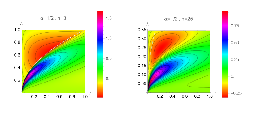
(a) Plots of $(r,\lambda)\mapsto(n)^{3/2}\,2\lambda\mathrm{cov}(r;\lambda^{2})$ for the Laguerre ensemble: $\alpha=1/2$. (Left): $n=3$, (Right): $n=25$.

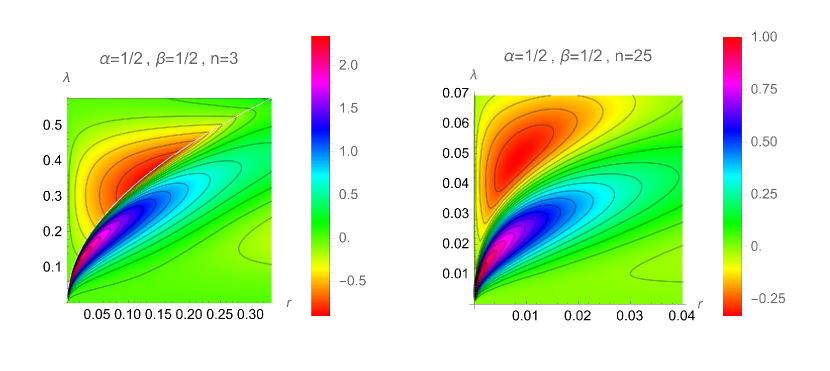
(b) Plots of $(r,\lambda)\mapsto 2\lambda\mathrm{cov}(r;\lambda^{2})$ for the Jacobi ensemble: $\alpha=1/2$, $\beta=1/2$. (Left): $n=3$, (Right): $n=25$.

Figure 1: Contour plots of the covariance density for a Laguerre (fig.1(a)) and a Jacobi (fig.1(b)) ensemble for the two matrix dimensions $n=3$ and $n=25$. See Eqs. (5.5) and (5.6) for the corresponding weight functions and their parameters $\alpha$ and $\beta$, respectively. We zoomed into the scale of the local mean level spacing for the singular values $\lambda$ and squared eigenradii $r$. The impact of line $\lambda=\sqrt{r}$, where the the covariance density is not smooth, is still visible for $n=3$ but becomes hard to detect for larger matrix dimensions.

We recall that the Dirac delta function $\delta(r_{1}r_{2}-a_{1}a_{2})$ reflects the identity (1.3). considering the SEV transform (2.7) one can conjecture that the conditional joint probability density of the eigenvalues is given in a distributional way by

$$\begin{split}d\mu_{n,n}(z|a)=&\frac{\prod_{j=0}^{n-1}j!}{(n!)^{2}\pi^{n}}|\Delta_{n}(z)|^{2}dz\lim_{\varepsilon\to 0}\int_{\mathcal{C}(n)}\left[\prod_{k=1}^{n}\frac{ds_{k}}{2\pi i}\zeta(\varepsilon\Im{s_{k}})\right]\\ &\times\mathrm{Perm}[|z_{b}|^{-2s_{c}}]_{b,c=1}^{n}\frac{\det[a_{b}^{s_{c}-1}]_{b,c=1}^{n}}{\Delta_{n}(s)\Delta_{n}(a)}\end{split}$$ (6.12)

The condition (1.3) is then still encoded in the integral over $s$ and the limit $\varepsilon\to 0$. At the moment a rigorous mathematical proof is missing for this conjecture because the $\varepsilon\to 0$ cannot exist point-wise but has to be understood in a distributional way.

Reversing the conditional probability measure, meaning finding the measure for the squared singular by conditioning the eigenvalues, is expected to be more challenging when considering the inverse SEV transform, see [32, Eq. (3.4)].

Our results for polynomial ensembles and especially for Pólya ensembles allow to study the large $n$ limit for cross-correlations of eigenvalues and singular values. For instance, it allows to analyse finite $n$ corrections of Feinberg-Zee’s Single Ring Theorem [22], rigorously proven in [25], for which some hard-to-check condition has then been lifted by [45]. The same holds for the Haagerup-Larsen Theorem [28] which relates the probability density of the eigenradii with those of the singular values. The finite $n$ analogue is encoded in Theorem 1.2. Especially the explicit formula (1.20) will enable us to understand how the asymptotics described by these theorems are approached.

Recently, a deformed Single Ring Theorem has been proven in [29]. It arises when the bi-unitary invariance is perturbed. Some kind of such perturbations might be also possible to study with our methods, as already pointed out in [32, Sec. 3.3].

There will be also interesting local spectral statistics of the cross-correlations between the complex eigenvalues and singular value. For instance the condition (1.6), implies non-trivial correlations when an edge of the eigenradii and the singular values agree. Such situation seems to be realised at the hard edge limit. In Fig. 1, we show contour plots of the covariance density $2\lambda{\rm cov}(r;\lambda^{2})$ for a Laguerre and a Jacobi ensemble with the same parameter $\alpha$, see Eqs. (5.5) and (5.6), for which we know they share the same hard edge statistics of the singular values. We have chosen the singular values $\lambda$ instead of the squared singular values $a=\lambda^{2}$ as then the scaling in $n$ of the mean level spacing agrees with the one of the squared eigenradii.

The contour plots for the matrix dimension $n=25$ show two things. Firstly, non-trivial (non-factorising) spectral statistics seem to emerge in the hard edge limit. Secondly these statistics seem to be universal as they appear to match for the two ensembles apart from a scaling. We will investigate this in a follow-up work.

References

• \bibcommenthead
• Akemann and Burda [2012] Akemann, G., Burda, Z.: Universal microscopic correlation functions for products of independent Ginibre matrices. Journal of Physics A: Mathematical and Theoretical 45(46), 465201 (2012) https://doi.org/10.1088/1751-8113/45/46/465201 arXiv:1208.0187
• Akemann et al. [2015] Akemann, G., Baik, J., Di Francesco, P.: The Oxford Handbook of Random Matrix Theory. Oxford University Press, Oxford (2015). https://doi.org/10.1093/oxfordhb/9780198744191.001.0001
• Akemann et al. [2014] Akemann, G., Burda, Z., Kieburg, M., Nagao, T.: Universal microscopic correlation functions for products of truncated unitary matrices. Journal of Physics A: Mathematical and Theoretical 47(25), 255202 (2014) https://doi.org/10.1088/1751-8113/47/25/255202 arXiv:1310.6395
• Ameur et al. [2023] Ameur, Y., Charlier, C., Moreillon, P.: Eigenvalues of truncated unitary matrices: disk counting statistics (2023) arXiv:2305.08976 [math-ph]
• Anderson et al. [2010] Anderson, G., Guionnet, A., Zeitouni, O.: An Introduction to Random Matrices. Cambridge studies in advanced mathematics 118. Cambridge university press, Cambridge (2010)
• Akemann and Ipsen [2015] Akemann, G., Ipsen, J.R.: Recent exact and asymptotic results for products of independent random matrices. Acta Physica Polonica B 46(9), 1747 (2015) https://doi.org/10.5506/aphyspolb.46.1747 arXiv:1502.01667
• Akemann et al. [2013] Akemann, G., Ipsen, J.R., Kieburg, M.: Products of rectangular random matrices: Singular values and progressive scattering. Physical Review E 88(5) (2013) https://doi.org/10.1103/physreve.88.052118 arXiv:1307.7560
• Akemann et al. [2013] Akemann, G., Kieburg, M., Wei, L.: Singular value correlation functions for products of Wishart random matrices. Journal of Physics A: Mathematical and Theoretical 46(27), 275205 (2013) https://doi.org/10.1088/1751-8113/46/27/275205 arXiv:1303.5694
• Andreev [1886] Andreev, K.A.: Note sur une relation entre les intégrales définies des produits des fonctions. Mémoires de la Societé des Sciences physiques et naturelles de Bordeaux (1886)
• Byun and Forrester [2023a] Byun, S.-S., Forrester, P.J.: Progress on the study of the Ginibre ensembles I: GinUE (2023) arXiv:2211.16223 [math-ph]
• Byun and Forrester [2023b] Byun, S.-S., Forrester, P.J.: Progress on the study of the Ginibre ensembles II: GinOE and GinSE (2023) arXiv:2301.05022 [math-ph]
• Bardenet et al. [2021] Bardenet, R., Ghosh, S., Lin, M.: Determinantal point processes based on orthogonal polynomials for sampling minibatches in SGD. Advances in Neural Information Processing Systems, 16226–16237 (2021) https://doi.org/10.48550/arXiv.2112.06007 arXiv:2112.06007 [stat.ML]
• Bianchi et al. [2021] Bianchi, E., Hackl, L., Kieburg, M.: Page curve for fermionic Gaussian states. Physical Review B 103(24) (2021) https://doi.org/%****␣main.bbl␣Line␣225␣****10.1103/physrevb.103.l241118 arXiv:2103.05416
• Braun et al. [2022] Braun, P., Hahn, N., Waltner, D., Gat, O., Guhr, T.: Winding number statistics of a parametric chiral unitary random matrix ensemble. Journal of Physics A Mathematical General 55(22), 224011 (2022) https://doi.org/10.1088/1751-8121/ac66a9 arXiv:2112.14575 [math-ph]
• Bhosale et al. [2018] Bhosale, U.T., Tekur, S.H., Santhanam, M.S.: Scaling in the eigenvalue fluctuations of correlation matrices. Phys. Rev. E 98, 052133 (2018) https://doi.org/10.1103/PhysRevE.98.052133 arXiv:1807.07968
• Deift and Gioev [2009] Deift, P., Gioev, D.: Random Matrix Theory: Invariant Ensembles and Universality. Courant Lecture Notes. American Mathematical Soc., New York (2009)
• Duistermaat and Kolk [2010] Duistermaat, J.J., Kolk, J.A.C.: Distributions: Theory and Applications, 1st edn. Cornerstones. Birkhäuser Boston, Boston, MA (2010)
• Dyson [1962] Dyson, F.J.: Statistical theory of the energy levels of complex systems. III. Journal of Mathematical Physics 3(1), 166–175 (1962) https://doi.org/10.1063/1.1703775
• Forrester et al. [2018] Forrester, P.J., Ipsen, J.R., Liu, D.-Z.: Matrix product ensembles of Hermite type and the hyperbolic Harish-Chandra-Itzykson-Zuber integral. Annales Henri Poincaré 19, 1307–1348 (2018) https://doi.org/10.1007/s00023-018-0654-x arXiv:1702.07100
• Förster et al. [2020] Förster, Y.-P., Kieburg, M., Kösters, H.: Polynomial ensembles and Pólya frequency functions. Journal of Theoretical Probability 34(4), 1917–1950 (2020) https://doi.org/10.1007/s10959-020-01030-z arXiv:1710.08794
• Forrester [2010] Forrester, P.J.: Log-Gases and Random Matrices (LMS-34). Princeton University Press, Princeton (2010). https://doi.org/10.1515/9781400835416
• Feinberg and Zee [1997a] Feinberg, J., Zee, A.: Non-Gaussian non-hermitian random matrix theory: Phase transition and addition formalism. Nuclear Physics B 501(3), 643–669 (1997) https://doi.org/10.1016/s0550-3213(97)00419-7 arXiv:cond-mat/9704191
• Feinberg and Zee [1997b] Feinberg, J., Zee, A.: Non-Hermitian random matrix theory: Method of Hermitian reduction. Nuclear Physics B 504(3), 579–608 (1997) https://doi.org/10.1016/s0550-3213(97)00502-6 arXiv:cond-mat/9703087
• Ghosh [2015] Ghosh, S.: Determinantal processes and completeness of random exponentials: the critical case. Probab. Theory Relat. Fields 163, 643–665 (2015) https://doi.org/10.48550/arXiv.1211.2435 arXiv:1211.2435 [math.PR]
• Guionnet et al. [2009] Guionnet, A., Krishnapur, M., Zeitouni, O.: The single ring theorem. Annals of Mathematics 174, 1189–1217 (2009) https://doi.org/10.4007/annals.2011.174.2.10 arXiv:0909.2214v2
• Hahn et al. [2023a] Hahn, N., Kieburg, M., Gat, O., Guhr, T.: Winding number statistics for chiral random matrices: Averaging ratios of determinants with parametric dependence. Journal of Mathematical Physics 64(2), 021901 (2023) https://doi.org/10.1063/5.0112423 arXiv:2207.08612 [math-ph]
• Hahn et al. [2023b] Hahn, N., Kieburg, M., Gat, O., Guhr, T.: Winding number statistics for chiral random matrices: Averaging ratios of parametric determinants in the orthogonal case. Journal of Mathematical Physics 64(11), 111902 (2023) https://doi.org/10.1063/5.0164352 arXiv:2306.12051 [math-ph]
• Haagerup and Larsen [2000] Haagerup, U., Larsen, F.: Brown’s spectral distribution measure for R-diagonal elements in finite von Neumann algebras. Journal of Functional Analysis 176(2), 331–367 (2000) https://doi.org/10.1006/jfan.2000.3610
• Ho and Zhong [2023] Ho, C.-W., Zhong, P.: Deformed single ring theorems (2023) arXiv:2210.11147 [math.PR]
• Ipsen [2015] Ipsen, J.R.: Products of independent Gaussian random matrices (2015) arXiv:1510.06128 [math-ph]
• Kieburg [2022] Kieburg, M.: Hard edge statistics of products of Pólya ensembles and shifted GUE’s. Journal of Approximation Theory 276, 105704 (2022) https://doi.org/10.1016/j.jat.2022.105704 arXiv:1909.04593v4
• Kieburg and Kösters [2016] Kieburg, M., Kösters, H.: Exact relation between singular value and eigenvalue statistics. Random Matrices: Theory and Applications 05(04), 1650015 (2016) https://doi.org/10.1142/s2010326316500155 arXiv:1601.02586
• Kieburg et al. [2015] Kieburg, M., Kuijlaars, A.B.J., Stivigny, D.: Singular value statistics of matrix products with truncated unitary matrices. International Mathematics Research Notices 2016(11), 3392–3424 (2015) https://doi.org/10.1093/imrn/rnv242 arXiv:1501.03910
• Kuijlaars and Stivigny [2014] Kuijlaars, A.B.J., Stivigny, D.: Singular values of products of random matrices and polynomial ensembles. Random Matrices: Theory and Applications 03(03), 1450011 (2014) https://doi.org/10.1142/S2010326314500117 arXiv:0909.2214
• Kuijlaars [2016] Kuijlaars, A.B.J.: Transformations of Polynomial Ensembles. In: Modern Trends in Constructive Function Theory, vol. 661, pp. 253–268 (2016). https://doi.org/10.1090/conm/661 . https://arxiv.org/abs/1501.05506
• Kanazawa et al. [2011] Kanazawa, T., Wettig, T., Yamamoto, N.: Singular values of the Dirac operator in dense QCD-like theories. JHEP 12, 007 (2011) https://doi.org/10.1007/JHEP12(2011)007 arXiv:1110.5858 [hep-ph]
• Kanazawa et al. [2012] Kanazawa, T., Wettig, T., Yamamoto, N.: Singular values of the Dirac operator at nonzero density. PoS LATTICE2012, 087 (2012) https://doi.org/10.22323/1.164.0087 arXiv:1212.2141 [hep-lat]
• Kuijlaars and Zhang [2014] Kuijlaars, A.B.J., Zhang, L.: Singular values of products of Ginibre random matrices, multiple orthogonal polynomials and hard edge scaling limits. Communications in Mathematical Physics 332(2), 759–781 (2014) https://doi.org/10.1007/s00220-014-2064-3 arXiv:1308.1003
• Kieburg and Zhang [2023] Kieburg, M., Zhang, J.: Derivative principles for invariant ensembles. Advances in Mathematics 413, 108833 (2023) https://doi.org/10.1016/j.aim.2022.108833 arXiv:2007.15259v2
• Long et al. [2023] Long, Z., Li, Z., Lin, R., Qiu, J.: On singular values of large dimensional lag-$\tau$ sample auto-correlation matrices. Journal of Multivariate Analysis 197, 105205 (2023) https://doi.org/10.1016/j.jmva.2023.105205 arXiv:2202.12526
• Lal Mehta [2004] Lal Mehta, M.: Random Matrices, 3rd edn. Pure and applied mathematics series, vol. 142. Elsevier Science and Technology, San Diego (2004)
• Loubaton and Mestre [2021] Loubaton, P., Mestre, X.: Testing uncorrelation of multi-antenna signals using linear spectral statistics of the spatio-temporal sample autocorrelation matrix. In: 2021 IEEE Statistical Signal Processing Workshop (SSP), pp. 201–205 (2021). https://doi.org/10.1109/SSP49050.2021.9513815
• Narayanan et al. [2023] Narayanan, H., Sheffield, S., Tao, T.: Sums of GUE matrices and concentration of hives from correlation decay of eigengaps (2023) arXiv:2306.11514 [math.PR]
• Nowak and Tarnowski [2017] Nowak, M.A., Tarnowski, W.: Spectra of large time-lagged correlation matrices from random matrix theory. Journal of Statistical Mechanics: Theory and Experiment 2017(6), 063405 (2017) https://doi.org/10.1088/1742-5468/aa6504 arXiv:1612.06552
• Rudelson and Vershynin [2014] Rudelson, M., Vershynin, R.: Invertibility of random matrices: Unitary and orthogonal perturbations. Journal of the American Mathematical Society 27(2), 293–338 (2014) https://doi.org/10.1090/S0894-0347-2013-00771-7 arXiv:1206.5180
• Schwartz [1966] Schwartz, L.: Théorie des Distributions., 2nd edn. Publications de l’Institut de mathématique de l’Université de Strasbourg 9-10. Hermann, Paris (1966)
• Soshnikov [2002] Soshnikov, A.: Gaussian limit for determinantal random point fields. Ann. Probab. 30, 171–187 (2002) https://doi.org/10.48550/arXiv.math/0006037 arXiv:math/0006037 [math.PR]
• Thurner and Biely [2007] Thurner, S., Biely, C.: The eigenvalue spectrum of lagged correlation matrices. Acta Physica Polonica B 38, 4111–4122 (2007)
• Weyl [1949] Weyl, H.: Inequalities between the two kinds of eigenvalues of a linear transformation. Proceedings of the National Academy of Sciences of the United States of America 35(7), 408–411 (1949)
• Yao and Yuan [2022] Yao, J., Yuan, W.: On eigenvalue distributions of large autocovariance matrices. The Annals of Applied Probability 32(5), 3450–3491 (2022) https://doi.org/10.1214/21-AAP1764 arXiv:2011.09165