Quantum focusing conjecture in two-dimensional evaporating black holes

Akihiro Ishibashi^1,2, Yoshinori Matsuo¹, and Akane Tanaka¹

¹Department of Physics and ²Research Institute for Science and Technology,
Kindai University, Higashi-Osaka, Osaka 577-8502, Japan

We consider the quantum focusing conjecture (QFC) for two-dimensional evaporating black holes. The QFC is closely related to the behavior of the generalized entropy—the sum of the area entropy for a given co-dimension two surface and the entanglement entropy for quantum fields outside the area. In the context of the black hole evaporation, the entanglement entropy of the Hawking radiation is decreasing after the Page time, and therefore it is not obvious whether the QFC holds in the black hole evaporation process especially after the Page time. One of the present authors previously addressed this problem in a four-dimensional spherically symmetric dynamical black hole model and showed that the QFC is satisfied. However the background spacetime considered was approximated by the Vaidya metric, and quantum effects of matters in the semiclassical regime is not fully taken into consideration. It remains to be seen if the QFC in fact holds for exact solutions of the semiclassical Einstein equations. In this paper, we address this problem in a two-dimensional dynamical black hole of the Russo-Susskind-Thorlacius (RST) model, which allows us to solve the semiclassical equations of motion exactly. We first give a suitable definition of the quantum expansion in two-dimensions and then prove that the QFC is satisfied for evaporating black holes in the RST model with the island formation taken into account.

1 Introduction

In general relativity, the focusing theorem is key to understanding the basic properties of gravitation. By combining the Raychaudhuri equation and certain energy conditions, the focusing theorem plays a central role in establishing various important results in general relativity, such as the singularity theorems [1]. For example, the black hole second law or the area theorem is based on the null focusing theorem, which asserts that under the null energy condition (NEC), the expansion $\theta$ of a null geodesic congruence is non-increasing:

$$\frac{d\theta}{d\lambda}\leq 0\,,$$ (1.1)

where $\lambda$ is an affine parameter of a null geodesic, say $\gamma$, and

$$\theta:=\dfrac{1}{{\cal A}}\dfrac{d{\cal A}}{d\lambda}\,,$$ (1.2)

with $\cal{A}$ being the sectional area of the null congruence including $\gamma$. Then, applying this theorem to a black hole with $\cal A$ regarded as the horizon area and using global techniques in general relativity, one can show that

$$d{\cal A}\geq 0\,.$$ (1.3)

However, when quantum effects are considered, the null focusing theorem does not in general hold due to the violation of the NEC.

As an alternative notion which is applicable even to the semiclassical regime, the quantum focusing conjecture (QFC) has been proposed [20]. The basic idea of the QFC is motivated from Bekenstein’s generalized entropy $S_{\rm gen}$, defined as [18, 19],

$$S_{\text{gen}}=\frac{{\cal A}}{4G_{N}}+S_{\text{out}}\,,$$ (1.4)

where $S_{\text{out}}$ is the von Neumann entropy of matter fields or radiation outside the black hole. As a semiclassical generalization of the classical area law (1.3), the generalized second law (GSL) asserts that $S_{\text{gen}}$ is non-decreasing:

$$dS_{\text{gen}}\geq 0\,.$$ (1.5)

Then, by using the generalized entropy, the null focusing theorem (1.1) is refined to the QFC [20], which states:

$$\frac{d\Theta}{d\lambda}\leq 0\,,$$ (1.6)

with $\Theta$—called the quantum expansion—being defined as a quantum generalization of the expansion (1.2). For the present context, $\Theta$ is given by

$$\Theta=\frac{4G_{N}}{{\cal A}}\frac{dS_{\text{gen}}}{d\lambda}\,.$$ (1.7)

The formula (1.6) with (1.7) applies not only for a black hole horizon as discussed above but also for any co-dimension two surface with the area ${\cal A}$ on a Cauchy hypersurface, for which $S_{\rm out}$ in (1.4) is given as the entanglement entropy for quantum fields on one side of the Cauchy hypersurface divided by the surface.

The QFC has been shown to hold in various situations in which quantum field effects violate the classical null focusing theorem. It is expected that the QFC can be used to establish many important results in semiclassical quantum gravity, just like the classical focusing theorem is in general relativity. For instance, the QFC is used to derive the quantum null energy condition (QNEC) [63, 64, 65], which is a quantum generalization of the NEC.

One of the most important problems in quantum gravity is the black hole information paradox. The black hole evaporation due to Hawking radiation implies that an initial pure quantum state forming a black hole appears to evolve into a mixed state. This picture, however, contradicts the unitary evolution in quantum theory, provided that the Hawking radiation is perfectly thermal and the black hole evaporates completely. A key for resolving this paradox is the Page curve [27, 28], which describes the behavior of the entanglement entropy of the Hawking radiation under quantum unitary evolution: the entanglement entropy initially monotonically increasing should turn to decrease at some point—called the Page time—and eventually vanishes at the end of the evaporation. One of the recent advances along this line is the proposal of the so called “island” [21, 22, 23, 24, 25, 26] which is a certain region supposed to host part of the degrees of freedom of the Hawking radiation in late time, despite being typically located inside the evaporating black hole. By using the idea of islands, a number of studies have been done [29, 30, 31, 32, 33, 34, 35, 36, 37, 38, 39, 40, 41, 42, 43, 44, 45, 46, 47, 48, 49, 50, 51, 52, 53].

It is of considerable interest in studying possible roles of the QFC in the context of the black hole information paradox, as the QFC closely connects classical geometry and quantum field effects. However, according to the above observation on a Page curve and an island formation, both the entanglement entropy of the Hawking radiation and the area of the evaporating black hole horizon decrease after the Page time. This begs the question of whether or not the QFC holds in the course of black hole evaporation, in particular, after the Page time.

One of the present authors previously considered this issue in a four-dimensional spherically symmetric model [54]. It is in general very hard to setup the background geometry describing a black hole evaporation by solving the semiclassical Einstein equations. First of all, the vacuum expectation value $\langle T_{\mu\nu}\rangle$ of stress-energy tensor for an arbitrary background spacetime is necessary to construct the semiclassical Einstein equations. It is practically difficult to calculate $\langle T_{\mu\nu}\rangle$ for quantum fields in four-dimension. Second, even when an expression of $\langle T_{\mu\nu}\rangle$ is obtained, solving the semiclassical Einstein equations is still a difficult task due to the fact that $\langle T_{\mu\nu}\rangle$ involves, in general, higher order derivatives. For these reasons, the analysis of [54] has been done by making several assumptions to sufficiently simplify the problem. In particular, the background geometry is not a solution of the semiclassical Einstein equations but quantum effects of matter are only partially taken into account: the Vaidya metric was exploited to include the negative incoming energy of quantum vacuum state, on which the QFC was shown to be satisfied. However, it is not clear whether such a background model can be justified in the semiclassical context.

In order to critically examine the QFC, it is most desirable to consistently solve the semiclassical Einstein equations. This is a formidable task as explained above, but can be undertaken—in fact, analytically—in two dimensions. It is well known that two dimensional gravity with dilaton fields [59, 60, 33] admits non-trivial dynamical black hole solutions, which enjoy many of the features of black holes in four-dimensions, such as the uniqueness and thermodynamic analogy [62]. In this paper, we consider the two-dimensional Russo-Susskind-Thorlacius (RST) dilaton gravity [60], whose semiclassical Einstein equation is solvable analytically, and show that the QFC indeed holds for dynamical black holes in the entire course of the Hawking evaporation with the island formation taken into consideration.

This paper is organized as follows. In the next section, we briefly review the black hole solutions in the two-dimensional gravity and generalized entropy with and without an island based on [33]. Then, in section 3, we prove that the quantum focusing conjecture holds in two dimensional evaporating black hole. In section 4, we present conclusion and outlook.

2 2D black holes and Islands

In this section, we briefly review two-dimensional black holes in the Callan-Giddings-Harvey-Strominger (CGHS) model and the RST model [59, 60, 33].

2.1 CGHS black holes

We first consider the CGHS model[59], in which black holes are studied in the two-dimensional dilaton gravity with the classical action given by [55, 56, 57, 58, 59]

$$I_{\text{CGHS}}=\frac{1}{2\pi}\int d^{2}x\sqrt{-g}e^{-2\phi}\{R+4(\nabla\phi)^{2}+4\lambda^{2}\}\,,$$ (2.1)

where $\phi$ is a dilaton field and $\lambda$ is a parameter characterizing the length scale. We can set $\lambda=1$ by an appropriate rescaling of two-dimensional coordinates. We further introduce matter fields without the dilaton coupling, and then, the equations of motion are

$$4e^{-2\phi}\left(\nabla_{\mu}\nabla_{\nu}\phi-g_{\mu\nu}\nabla^{2}\phi+g_{\mu\nu}(\nabla\phi)^{2}-g_{\mu\nu}\right)=T_{\mu\nu}\,,$$ (2.2)

$$R-4(\nabla\phi)^{2}+4\nabla^{2}\phi+4=0\,,$$ (2.3)

where $T_{\mu\nu}$ is the energy-momentum tensor of the matter fields. In the conformal gauge, the metric takes the following form:

$$ds^{2}=-e^{2\rho}dx^{+}dx^{-}\,,$$ (2.4)

where $\rho$ is a function of $x^{+}$ and $x^{-}$. The coordinates $x^{\pm}$ are called the Kruskal coordinates. We restrict matter fields to conformal matters, or equivalently, impose $T_{+-}=0$, and then, we can set $\rho(x^{+},x^{-})=\phi$ without loss of generality. The equations of motion (2.2) and (2.3) can be expressed as

$$-2\partial^{2}_{\pm}e^{-2\phi} =T_{\pm\pm}\,,$$ (2.5)

$$-\partial_{+}\partial_{-}e^{-2\phi} =1\,,$$ (2.6)

respectively.

2.1.1 Static black holes

We first consider static solutions of the two-dimensional dilaton gravity theory. The simplest solution of eq. (2.6) is given by

$$e^{-2\phi}=-x^{+}x^{-}\,.$$ (2.7)

Then, the metric is given by

$$ds^{2}=\frac{dx^{+}dx^{-}}{x^{+}x^{-}}\ ,$$ (2.8)

which is nothing but flat spacetime. In order to see this more explicitly, we introduce the coordinates $(\sigma^{+},\sigma^{-})$ which are defined by $x^{+}=e^{\sigma^{+}}$ and $x^{-}=e^{\sigma^{-}}$. Then, the metric takes the standard form of flat spacetime in double null coordinates:

$$ds^{2}=-d\sigma^{+}d\sigma^{-}\,.$$ (2.9)

The other equation of motion (2.5) determines the energy-momentum tensor in this solution and gives $T_{++}=T_{--}=0$. Thus, this solution is a vacuum solution. Since the dilaton is proportional to the spatial coordinate $\sigma=\frac{1}{2}(\sigma^{+}-\sigma^{-})$:

$$\phi=-\sigma\,,$$ (2.10)

this solution is called a linear dilaton vacuum solution.

A non-dynamical black hole solution is given by

$$e^{-2\phi}=M-x^{+}x^{-}\,,$$ (2.11)

where $M$ is an integration constant and proportional to the black hole mass. When $M>0$, the event horizon is located at $x^{+}x^{-}=0$. For $M>0$, we introduce the rescaled coordinates, $v=x_{+}/\sqrt{M}$ and $u=x_{-}/\sqrt{M}$ so that the black hole solution becomes

$$ds^{2}=-\frac{dvdu}{1-vu}\,,$$ (2.12)

with a curvature singularity at $uv=1$ and the event horizon at $uv=0$. It is straightforward to see that this black hole solution is asymptotically flat by using the coordinates $(\sigma^{+},\sigma^{-})$. The global structure of this solution is essentially the same as that of the two-dimensional part of the Schwarzschild black hole.

2.1.2 Dynamical black holes

Next, we consider dynamical solutions. The most general solution of the equation of motion (2.6) is given by

$$e^{-2\phi}=-x^{+}x^{-}+A(x^{+})+B(x^{-})\,,$$ (2.13)

where $A(x^{+})$ and $B(x^{-})$ are integration constants. We introduce an ingoing shock wave at $x^{+}=x^{+}_{0}$ and assume that there is no other excitation of matter fields. Then, the energy momentum tensor is given by

$$T_{++}=a\delta(x^{+}-x^{+}_{0})\,,\quad T_{--}=0\,,$$ (2.14)

where $a$ is the magnitude of the shock wave. By imposing the initial condition that the solution is given by the linear dilaton vacuum solution before the shock wave and integrating (2.5), $A(x^{+})$ and $B(x^{-})$ can be calculated as

$$A(x^{+})=-\frac{a}{2}(x^{+}-x^{+}_{0})\theta(x^{+}-x^{+}_{0})\,,\quad B(x^{-}) =0\,.$$ (2.15)

Then, we have obtained the following solution,

$$e^{-2\phi(x^{+},x^{-})}=e^{-2\rho(x^{+},x^{-})}=\left\{\begin{array}[]{ll}-x^{+}x^{-}&\text{if}\,\,x^{+}<x^{+}_{0}\,,\\ M-x^{+}\Big{(}x^{-}+\frac{M}{x^{+}_{0}}\Big{)}&\text{if}\,\,x^{+}>x^{+}_{0}\,,\end{array}\right.$$ (2.18)

where we have chosen $M=ax^{+}_{0}/2$.

Let us look at the properties of the two solutions. In the case $x^{+}<x^{+}_{0}$, i.e. before the incoming shock wave, the solution is the linear dilaton vacuum solution discussed above. In the case $x^{+}>x^{+}_{0}$, i.e. after incoming shock wave, the metric is expressed as

$$ds^{2} =\dfrac{1}{M-x^{+}\left(x^{-}+\dfrac{M}{x^{+}_{0}}\right)}dx^{+}dx^{-}=\frac{1}{1-v(u+1)}dudv\,.$$ (2.19)

Here, we have made the coordinate transformation

$$x^{+}=x^{+}_{0}v\,,\qquad x^{-}=\frac{M}{x^{+}_{0}}u\,.$$ (2.20)

This is the black hole solution whose event horizon is now located at $v(u+1)=0$ and whose curvature singularity is at $v(u+1)=1$. Thus, we have obtained a classical solution that describes an evolution from the linear dilaton vacuum (2.8) to the black hole spacetime (2.19).

2.1.3 Quantum energy-momentum tensor

Next, we take into account quantum corrections of matter fields on the spacetime dynamics. As it is too complicated to calculate directly the expectation value of the energy-momentum tensor, we determine the value by using the conservation law and anomaly condition. The energy-momentum tensor of conformal matters is traceless at classical level, but has the conformal anomaly for curved background when quantum effects are taken into consideration:

$$\langle T^{\mu}{}_{\mu}\rangle=\frac{c}{12}R\,,$$ (2.21)

where $R$ is the Ricci scalar of background spacetime and $c$ is central charge, which is assumed to obey $M\ll c$ in this paper. In the double null coordinates $(x^{+},x^{-})$ or $(u,v)$, eq. (2.21) is expressed as

$$\langle T_{+-}\rangle=-\frac{c}{6}\partial_{+}\partial_{-}\rho\,.$$ (2.22)

The other components can be calculated by integrating the conservation law $\nabla^{\mu}T_{\mu\nu}=0$ as

$$\langle T_{\pm\pm}\rangle=\frac{c}{12}\left[2\partial^{2}_{\pm}\rho-2(\partial_{\pm}\rho)^{2}+t_{\pm}\right]\,,$$ (2.23)

where $t_{\pm}(x_{\pm})$ are integration constants determined by physical boundary conditions.

Now, we compute the energy-momentum tensor to see Hawking radiation in the situation where a matter field undergoes a gravitational collapse to form a black hole. The metric is the same as in (2.18) with the coordinates (2.20). In the case $v<1$, the energy momentum tensor is zero because it is linear dilaton vacuum. By using the expression of the metric (2.8), we obtain

$$t_{-}(u)=-\frac{1}{2u^{2}}\,.$$ (2.24)

Since $t_{-}(u)$ is independent of $v$, the energy-momentum tensor for $v>1$ is calculated by using (2.24) as

$$T_{uu}=\frac{v^{2}}{2\left[1-v(u+1)\right]^{2}}-\frac{1}{2u^{2}}\,.$$ (2.25)

In the coordinates $v=e^{\sigma^{+}},u=-1-e^{-\sigma^{-}}$, the metric can be expressed as

$$ds^{2}=-\frac{1}{1+e^{\sigma^{-}-\sigma^{+}}}d\sigma^{+}d\sigma^{-}\,.$$ (2.26)

This is asymptotically flat. If outgoing energy flux is calculated at $\sigma^{+}\rightarrow\infty$, it is expressed by

$$T_{\sigma^{-}\sigma^{-}}(\sigma)\simeq\frac{c}{24}\left\{1-\frac{1}{(1+e^{\sigma^{-}})^{2}}\right\}\,.$$ (2.27)

This corresponds to Hawking radiation and implies that the black hole loses its mass.

It should be noted that $t_{\pm}$ transforms under the coordinate transformation as

$$\left(\frac{\sigma^{\pm}}{w^{\pm}}\right)^{2}t_{\pm}(\sigma^{\pm})=t_{\pm}(w^{\pm})+\{\sigma^{\pm},w^{\pm}\}\ ,$$ (2.28)

where

$$\{f(x),x\}=\frac{f^{\prime\prime\prime}}{f^{\prime}}-\frac{3}{2}\frac{\left(f^{\prime\prime}\right)^{2}}{\left(f^{\prime}\right)^{2}}$$ (2.29)

is the Schwarzian derivative. If we take the coordinates $v=e^{\omega^{+}},u=-e^{-\omega^{-}}$ for $v<1$, the metric reduces to the flat metric $ds^{2}=-d\omega^{+}d\omega^{-}$. From $\rho(\omega^{+},\omega^{-})=0$, we find $t_{-}(\omega^{-})=0$. For $v>1$, we still have $\rho\simeq 0$ in $\sigma^{+}\to\infty$, and the outgoing energy flux is $T_{\sigma^{-}\sigma^{-}}(\sigma)\simeq({c}/{12})t_{-}(\sigma^{-})$. Then, eq. (2.27) can also be reproduced by using the transformation (2.28).

2.2 RST black holes

We consider the semiclassical black hole geometry—how the black hole geometry is modified by the back reaction of quantum effects. The semiclassical geometry can be calculated by solving semiclassical equations of motion: (2.5)–(2.6) with (2.22)–(2.23), but no analytic expression of exact black hole solutions have been found. This problem would be related to the fact that the quantum energy-momentum tensor (2.22)–(2.23) breaks a symmetry of the model (2.1):

$$\delta\phi=\delta\rho=\varepsilon e^{2\phi}\,.$$ (2.30)

In order to avoid this problem, we resort to the RST model [60]. The quantum energy-momentum tensor (2.22)–(2.23) can be reproduced by adding the following non-local Polyakov term to the action $I_{\text{CGHS}}$, (2.1):

$$I_{Q}=-\frac{c}{12\pi}\int dx^{+}dx^{-}\partial_{+}\rho\partial_{-}\rho\,.$$ (2.31)

In order to preserve the symmmetry (2.30), we further modify the action by adding the following term [60],

$$I_{\text{RST}}=\frac{c}{48\pi}\int d^{2}x\sqrt{-g}\phi R\,.$$ (2.32)

Following [60, 61], we introduce a new field variable:

$$\Omega=e^{-2\phi}+\frac{c}{24}\phi\,,$$ (2.33)

which significantly simplifies the field equations. The field variable $\Omega$ takes a lower bound at $\Omega=\Omega_{\text{crit}}=({c}/{48})[1-\log({c}/{48})]$, which corresponds to the boundaries of spacetime. The field equations for the action $I_{\text{CGHS}}+I_{\text{Q}}+I_{\text{RST}}$ can be expressed as

$$\partial_{+}\partial_{-}\Omega+1=0\,,\qquad-\partial_{\pm}^{2}\Omega=\frac{c}{24}t_{\pm}\,,$$ (2.34)

where $t_{\pm}$ is the same integration constants as before.

Noted that $t_{+}$ is not the energy-momentum tensor. Taking the additional term (2.32) into account, the off-diagonal component of the equation of motion (2.2) is modified as

$$\left(e^{-2\phi}-\frac{c}{48}\right)\left[\partial_{\pm}^{2}\phi-2\partial_{\pm}\rho\partial_{\pm}\phi\right]=-\frac{1}{2}T_{\pm\pm}\ ,$$ (2.35)

where $T_{\pm\pm}$ is the expectation value of the energy-momentum tensor, which contains contributions from the conformal anomaly.

2.2.1 Linear dilaton vacuum

The linear dilaton vacuum solution takes the form

$$\Omega=-x^{+}x^{-}-\frac{c}{48}\log(-x^{+}x^{-})\,,$$ (2.36)

where we have assumed $T_{\pm\pm}=0$. Substituting the solution $\Omega$ into the second equation of (2.34), we find that

$$t_{\pm}=-\frac{1}{2}\frac{1}{(x^{\pm})^{2}}\,.$$ (2.37)

The metric can be read off from (2.33) and is expressed as

$$ds^{2}=\frac{1}{x^{+}x^{-}}dx^{+}dx^{-}\,.$$ (2.38)

This is a vacuum solution written in the Kruskal coordinates.

2.2.2 Two-sided eternal black hole

The eternal black hole solution is given by

$$\Omega=M(1-uv)+\Omega_{\text{crit}}\,,$$ (2.39)

where the coordinate system was set to $x^{+}=\sqrt{M}v,\;x^{-}=\sqrt{M}u$. We find $t_{\pm}(x^{\pm})=0$ from (2.34). If the coordinate system is transformed to $v=e^{\sigma^{+}},\;u=-e^{-\sigma^{-}}$, we obtain $t_{\pm}(\sigma^{\pm})=1/2$, which can be expressed as $T_{\sigma^{\pm}\sigma^{\pm}}(\sigma^{\pm})={c}/{24}$ near the spatial infinity since $\rho\simeq 0$ and $T_{\sigma^{\pm}\sigma^{\pm}}\simeq ct_{\pm}(\sigma^{\pm})/12$ there. This implies that the black hole has the temperature $T={1}/{2\pi}$, which is independent of the mass.

2.2.3 Dynamical black hole

We consider a situation where a shock wave of matter fields is injected into a linear dilaton vacuum. Here, we assume that the classical part of the energy-momentum tensor is given by

$$T_{++} =\frac{2M}{x_{0}^{+}}\delta(x^{+}-x^{+}_{0})\,, T_{--} =0\,,$$ (2.40)

as in the evaporating black holes in the CGHS model. If we assume that the spacetime is flat in the infinite past, then

$$t_{\pm}(x^{\pm})=-\dfrac{1}{2}\dfrac{1}{(x^{\pm})^{2}}\,,$$ (2.41)

before the injection of the shock wave. Then, the solution $\Omega$ is expressed as

$$\Omega =-x^{+}x^{-}-\frac{c}{48}\log(-x^{+}x^{-})-\frac{M}{x_{0}^{+}}(x^{+}-x^{+}_{0})\theta(x^{+}-x^{+}_{0})$$

$$=M\left[1-v(u+1)-\epsilon\log(-Muv)\right]\,,$$ (2.42)

where we have introduced the expansion parameter $\epsilon:=c/48M\ll 1$.

2.3 Generalized entropy

The generalized entropy for an anchor point $A$ in a two-dimensional dynamical black hole, which divide a Cauchy surface to two regions, is expressed as [33]

$$S_{\text{gen}}=\frac{\text{Area(A)}}{4G_{N}}+\frac{\text{Area(I)}}{4G_{N}}+S_{\text{bulk}}[\mathcal{S}_{\text{AI}}]\,.$$ (2.43)

The first term on the right hand side corresponds to the area term in the higher dimensional cases, which is identified as

$$\frac{\text{Area}}{4G_{N}}=2(\Omega-\Omega_{\text{crit}})$$ (2.44)

for the RST model. In fact, $\Omega$ is the Noether charge or Wald entropy [66] derived from the action $I_{\text{CGHS}}+I_{Q}+I_{\text{RST}}$ as shown in [67]. This term was ignored in the study on the Page curve [33], but plays important role in the QFC. We will omit this term in this section, but take it into account explicitly in the next section. The second term is the area term at the boundary of the island, which is $2(\Omega(I)-\Omega_{\text{crit}})$, arises from effects of islands and vanishes if there is no island. The third term, $S_{\text{bulk}}$, is the von Neumann entropy of the CFT matter fields on (the complement of) a spacelike surface $\mathcal{S}_{AI}$, connecting the boundary of island $I$ and the anchor point $A$. The bulk entropy $S_{\text{bulk}}$ is expressed as

$$S_{\text{bulk}}[\mathcal{S}_{\text{AI}}]=\frac{c}{6}\log\left|d(A,I)^{2}e^{\rho\text{(A)}}e^{\rho\text{(I)}}\right|_{t_{\pm}=0}\,,$$ (2.45)

where $d(A,I)$ is the distance between the anchor curve and the island,

$$d(A,I)^{2}=\left|(x^{+}(A)-x^{+}(I))(x^{-}(A)-x^{-}(I))\right|^{2}\,.$$ (2.46)

The expressions above depend on the coordinate system, which should be chosen so that $t_{\pm}=0$. Here, the anchor curve is located far outside the black hole. The position of the island is determined so that the generalized entropy is extremized, and then, the island is placed inside the event horizon as we will see below. In the absence of islands, the surface $\mathcal{S}_{AI}$ extends from the anchor curve to the inner boundary of the spacetime defined by $\Omega=\Omega_{\text{crit}}$, and then, the position of the boundary of the island in the expressions above should be replaced accordingly. The situation we are considering is illustrated by Figure 1.

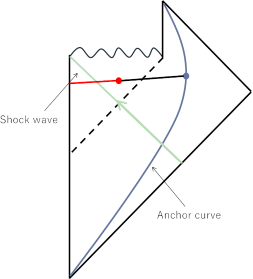
Figure 1: This is the Penrose diagram of the RST black hole. The red line represents the island and the blue line the anchor curve.

2.3.1 Island

The generalized entropy in the presence of an island is expressed as

$$S^{\text{island}}_{\text{gen}}= 2M\left\{1-v_{\text{I}}(1+u_{\text{I}})-\epsilon\log(-Mv_{\text{I}}u_{\text{I}})\right\}$$

$$+\frac{c}{12}\log\left[\Big{(}\log\frac{v_{\text{A}}}{v_{\text{I}}}\log\frac{u_{\text{A}}}{u_{\text{I}}}\Big{)}^{2}\frac{v_{\text{A}}u_{\text{A}}}{1-v_{\text{A}}(1+u_{\text{A}})}\frac{v_{\text{I}}u_{\text{I}}}{1-v_{\text{I}}(1+u_{\text{I}})}\right]\,.$$ (2.47)

To find the position of the island $(v_{I},u_{I})$, we extremize (2.47) over $(v_{I},u_{I})$ and obtain the following two conditions,

$$0 =-2M(1+u_{I})+\dfrac{c}{12v_{I}}\frac{1}{1-v_{I}(1+u_{I})}-\dfrac{c}{24v_{I}}-\dfrac{c}{6v_{I}{\log\left(\dfrac{v_{A}}{v_{I}}\right)}}\,,$$ (2.48)

$$0 =-2Mv_{I}+\dfrac{c}{12v_{I}}\dfrac{1-v_{I}}{1-v_{I}(1+u_{I})}-\dfrac{c}{24u_{I}}-\dfrac{c}{6v_{I}\log\left(\frac{u_{A}}{u_{I}}\right)}\,.$$ (2.49)

Here, we can drop the last term on the right side of (2.48), when $\log({v_{A}}/{v_{I}})\gg 1$. Let us see that this is indeed the case. Using (2.48) and (2.49), we obtain the following equations:

$$(v_{I}(1+u_{I}))^{2}-(1-\epsilon)v_{I}(1+u_{I})+\epsilon=0\,,\quad\log\frac{u_{A}}{u_{I}}=4(1+u_{I})\,.$$ (2.50)

Solving (2.50) for $v_{I}(1+u_{I})$, we obtain

$$u_{I}=-1+\frac{\epsilon}{v_{I}}+O(\epsilon^{2}).$$ (2.51)

The other solution is unphysical near the singularity. Substituting the island solution (2.51) into (2.50), we have

$$v_{I}=-\frac{3\epsilon}{(u_{A}+1)}+O(\epsilon^{2})\,.$$ (2.52)

Next, introducing

$$u_{A}=-1-e^{\sigma_{A}-t_{A}}\,,\qquad v_{A}=e^{\sigma_{A}+t_{A}}\,,$$ (2.53)

and using (2.52) and (2.53), we obtain

$$\log\frac{v_{A}}{v_{I}}\sim 2\sigma_{A}+\log\frac{1}{\epsilon}\gg 1\,.$$ (2.54)

Thus, $\log({v_{A}}/{v_{I}})\gg 1$ holds and the last term of (2.48) can be dropped. Finally, substituting (2.51) into (2.47), we obtain

$$S^{\text{island}}_{\text{gen}}=2M-\frac{c}{24}(t_{A}-\sigma_{A})+\frac{c}{6}\sigma_{A}+\cdots\,.$$ (2.55)

2.3.2 No-island

We consider the generalized entropy $S^{\text{no-island}}_{\text{gen}}$ in the absence of an island. Let the surface $\mathcal{S}_{AI}$ extend to a fixed reference point $(v_{0},u_{0})$ on the boundary $\Omega=\Omega_{\text{crit}}$ in the region $v<1$: i.e., $v_{0}<1$ and $u_{0}=-\epsilon/v_{0}$. Then, we can express the generalized entropy $S^{\text{no-island}}_{\text{gen}}$ as

$$S^{\text{no-island}}_{\text{gen}} =\frac{c}{12}\log\left[\left(\log\dfrac{v_{\text{A}}}{v_{\text{0}}}\log\dfrac{u_{\text{A}}}{u_{\text{0}}}\right)^{2}\dfrac{v_{\text{A}}u_{\text{A}}}{1-v_{\text{A}}(1+u_{\text{A}})}\right]$$

$$=\frac{c}{12}(t_{A}-\sigma_{A})+\frac{c}{6}\sigma_{A}+\cdots\,.$$ (2.56)

3 The quantum focusing conjecture in RST model

In this section, we show that the QFC holds for two-dimensional evaporating black holes in the RST model. We should first note that in two dimensions, there is a subtle issue in the definition of the quantum expansion, as a given co-dimension two surface—whose area $\cal A$ appears in the denominator of the original definition (1.7)—now corresponds to a single point in the two dimensional setting. This ambiguity is related to the facts that null geodesics can form no co-dimension two surface in two dimensions and that the notion of focusing in two dimension is unclear. A candidate of the quantum expansion might be simply

$$\Theta=\frac{dS_{\text{gen}}}{d\lambda}\,.$$ (3.1)

This definition however does not give desired properties of quantum focusing even in the classical limit. The counterpart of the classical expansion for (3.1) is simply given by

$$\theta=\frac{d}{d\lambda}e^{-2\phi}\,.$$ (3.2)

As the derivative with respect to the affine parameter can be rewritten as ${d}/{d\lambda}=e^{-2\rho}\partial_{+}$, the focusing condition is expressed in the gauge $\rho=\phi$ as

$$\frac{d\theta}{d\lambda}=e^{-2\phi}\left(\partial_{+}e^{-2\phi}\right)^{2}-\frac{1}{2}e^{-4\phi}T_{++}\,,$$ (3.3)

where we used (2.5). Thus, the definition (3.1) gives an increasing expansion even for $T_{++}=0$, and hence, is not a desirable definition of the quantum expansion.

By inspection, we find it appropriate to replace the geometric area ${\cal A}$ in (1.7) with the variable $\Omega=e^{-2\phi}+c\phi/24$ introduced in (2.33). In fact, we have already taken the perspective that $\Omega$ can be viewed as the “area” or geometric entropy with quantum correction to define the generalized entropy (2.43)–(2.44). Another piece of evidence for the correspondence between $\Omega$ in two-dimensions and the area entropy in higher-dimensions can be found in the derivation of two-dimensional black holes in the “large-$D$ expansion” in gravity [68, 69], where the area of the $(D-2)$-sphere in spherically symmetric spacetimes is identified with $e^{-2\phi}$ up to a constant factor. In view of this, we define the two-dimensional counterpart of the classical expansion (1.2) as

$$\theta:=e^{2\phi}\dfrac{d}{d\lambda}e^{-2\phi}\,,$$ (3.4)

which gives an analogue of the Raychaudhuri equation:

$$\frac{d\theta}{d\lambda}=-\frac{1}{2}e^{-2\phi}T_{++}\,.$$ (3.5)

Thus, the classical focusing theorem holds if the NEC is satisfied. The classical expansion (3.4) would naturally generalized for the RST model as

$$\theta:=\dfrac{1}{\Omega}\dfrac{d\Omega}{d\lambda}\,.$$ (3.6)

The derivative of the expansion is expressed in terms of the energy-momentum tensor (2.35) as

$$\frac{d\theta}{d\lambda}=-\left[1-\left(\frac{\Omega}{e^{-2\phi}-{c}/{48}}\right)^{2}\right]\theta^{2}-\frac{e^{-4\phi}}{2\Omega}T_{++}\ .$$ (3.7)

This corresponds to the Raychaudhuri equation for the classical expansion (3.6) with quantum correction. In the limit $c\to 0$, eq. (3.7) for the RST model reduces to eq. (3.5) for the CGHS model.

However, the classical focusing would be violated in the RST model. By using (2.34), we obtain

$$\dfrac{d\theta}{d\lambda}=-\frac{c}{24}\frac{\left(-\phi-{1}/{2}\right)}{\left(e^{-2\phi}-{c}/{48}\right)}\theta^{2}-\frac{1}{2}\frac{e^{-4\phi}}{\Omega}\left(T_{++}^{\text{(cl)}}+\frac{c}{12}t_{+}\right)\,,$$ (3.8)

where $T_{++}^{\text{(cl)}}$ is the classical part of the energy-momentum tensor. We can see from (3.8) that for two-sided eternal black hole, $t_{+}=0$, and the classical focusing ${d\theta}/{d\lambda}\leq 0$ holds as long as the quantum correction in $\Omega$ is sufficiently small, namely, for $e^{-2\phi}\gg{c}\phi/{24}$, since the first term in (3.8) is non-positive for $\phi<-{1}/{2}$, and non-positive for $\phi>-{1}/{2}$. If $c<48e$, $\phi>-{1}/{2}$ sufficiently near the boundary $\Omega=\Omega_{\text{crit}}$. Thus, the classical focusing ${d\theta}/{d\lambda}\leq 0$ holds for asymptotic region (large values of $\Omega$), while it could be violated for sufficiently small $\Omega$. For the linear dilation vacuum and dynamical black holes, $t_{+}<0$, we need more careful analysis. In any case, the violation of the classical focusing comes from quantum effects.

Now, we propose to define the quantum expansion in two-dimensions as follows:

$$\Theta:=\frac{1}{2\Omega}\frac{dS_{\text{gen}}}{d\lambda}\,.$$ (3.9)

Note that one can easily check that if $\Theta$ is defined without $\Omega$ in the denominator, the QFC for such defined $\Theta$ fails to hold, except for some circumstances [see, e.g., Case (ii) below].

As the generalized entropy $S_{\text{gen}}$ in the above definition (3.9), we consider two expressions: one $S^{\text{island}}_{\text{gen}}$ for island configuration and the other $S^{\text{no-island}}_{\text{gen}}$ for no island configuration, which we reviewed in the previous section. Restoring the area term at the anchor point, they are expressed as follows:

$$S^{\text{island}}_{\text{gen}}= 2M\left\{1-v_{\text{I}}(1+u_{\text{I}})-\epsilon\log(-Mv_{\text{I}}u_{\text{I}})\right\}$$

$$+2M\left\{1-v_{\text{A}}(1+u_{\text{A}})-\epsilon\log(-Mv_{\text{A}}u_{\text{A}})\right\}$$

$$+\frac{c}{12}\log\left[\left(\log\frac{v_{\text{A}}}{v_{\text{I}}}\log\frac{u_{\text{A}}}{u_{\text{I}}}\right)^{2}\frac{v_{\text{A}}u_{\text{A}}}{1-v_{\text{A}}(1+u_{\text{A}})}\frac{v_{\text{I}}u_{\text{I}}}{1-v_{\text{I}}(1+u_{\text{I}})}\right]\,,$$ (3.10)

$$S^{\text{no-island}}_{\text{gen}}= 2M\left\{1-v_{\text{A}}(1+u_{\text{A}})-\epsilon\log(-Mv_{\text{A}}u_{\text{A}})\right\}$$

$$+\frac{c}{12}\log\left[\left(\log\frac{v_{\text{A}}}{v_{\text{0}}}\log\frac{u_{\text{A}}}{u_{\text{0}}}\right)^{2}\frac{v_{\text{A}}u_{\text{A}}}{1-v_{\text{A}}(1+u_{\text{A}})}\right]\,,$$ (3.11)

where the position of (the boundary of) the island $(u_{I},v_{I})$ are given by (2.51)–(2.52), as we have seen in the previous section. Note that the area of the anchor curve is ignored in [33] as it is irrelevant constant for the Page curve, while it plays an important role in the quantum focusing conjecture.

We examine the behavior of these two entropies, $S^{\text{island}}_{\text{gen}}$ and $S^{\text{no-island}}_{\text{gen}}$, in the following three cases (i) $\epsilon\ll-v_{\text{A}}(1+u_{\text{A}})\ll 1$, (ii) $-v_{A}(1+u_{A})=O(1)$ and (iii) $-v_{A}(1+u_{A})\sim\epsilon$, separately. Our goal is to show, for each case of (i)–(iii),

$$\dfrac{\partial}{\partial v}\left[\left(\dfrac{e^{-2\rho}}{\Omega}\dfrac{\partial}{\partial v}S_{\rm gen}^{\text{island/no-island}}\right)\right]\leq 0\,.$$ (3.12)

3.1 Case (i): $\epsilon\ll-v_{\text{A}}(1+u_{\text{A}})\ll 1$

In this case, $\Omega$ can be approximated as

$$\Omega(A) \simeq M-\frac{c}{48}\log v_{A}\,,$$ (3.13)

$$\Omega(I) \simeq M+\frac{c}{48}\log(-1-u_{A})\,,$$ (3.14)

and the bulk entropy $S_{\text{bulk}}$ is

$$S_{\text{bulk}}^{\text{island}}\simeq\frac{c}{12}\log v_{A}+\frac{c}{12}\log(-1-u_{A})\,,$$ (3.15)

for the island configuration and

$$S_{\text{bulk}}^{\text{no-island}}\simeq\frac{c}{12}\log v_{A}\,,$$ (3.16)

for the no-island configuration. Using these relations, we can express $S^{\text{island}}_{\text{gen}},\,S^{\text{no-island}}_{\text{gen}}$ approximately as

$$S^{\text{island}}_{\text{gen}} \simeq 4M+\frac{c}{8}\log(-u_{A}-1)+\frac{c}{24}\log v_{A}\,,$$ (3.17)

$$S^{\text{no-island}}_{\text{gen}} \simeq 2M+\frac{c}{24}\log v_{A}\,.$$ (3.18)

3.1.1 GSL

Taking the derivative with respect to $v_{A}$, we find

$$\partial_{v_{\text{A}}}S^{\text{island}}_{\text{gen}}=\frac{c}{24}\frac{1}{v_{A}}\,,$$ (3.19)

$$\partial_{v_{\text{A}}}S^{\text{no-island}}_{\text{gen}}=\frac{c}{24}\frac{1}{v_{A}}\,,$$ (3.20)

both of which are non-negative. Therefore both $S_{\text{gen}}^{\text{island}}$ and $S_{\text{gen}}^{\text{no-island}}$ are non-decreasing.

3.1.2 QFC

Next, to see if the QFC holds, we check $\partial^{2}_{\lambda}S_{\text{gen}}\leq 0$. We have

$$\partial^{2}_{\lambda}S_{\text{gen}}=e^{-4\rho}(\partial^{2}_{+}S-2\partial_{+}\rho\partial_{+}S)\,.$$ (3.21)

Since $\Omega=e^{-2\rho}+{c}\rho/{24}=M+O(\epsilon)$ as we have seen in (3.13), it follows that $\partial_{+}\rho=O(\epsilon)$. As we have also found in (3.17)–(3.18) that $\partial_{+}S_{\text{gen}}=O(\epsilon)$, the second term is zero up to $O(\epsilon^{2})$ terms. The first term is calculated as

$$\partial^{2}_{+}S^{\text{island}}_{\text{gen}}=-\Big{(}\frac{\partial v_{\text{A}}}{\partial x^{+}}\Big{)}^{2}\frac{c}{24}\frac{1}{v^{2}_{\text{A}}}<0\,,$$ (3.22)

$$\partial^{2}_{+}S^{\text{no-island}}_{\text{gen}}=-\Big{(}\frac{\partial v_{\text{A}}}{\partial x^{+}}\Big{)}^{2}\frac{c}{24}\frac{1}{v^{2}_{\text{A}}}<0\,.$$ (3.23)

Thus, the QFC is satisfied,

$$\frac{d\Theta}{d\lambda}<0\,.$$ (3.24)

3.2 Case (ii): $-v_{A}(1+u_{A})=O(1)$

This case implies that $v_{\text{A}}$ and $v_{\text{I}}$ are far away from each other. By using (2.51)–(2.52), the generalized entropy can be approximately expressed as

$$S^{\text{island}}_{\text{gen}}\simeq\,\, 4M+\frac{c}{24}+\frac{c}{24}\log(u_{\text{A}}+1)-\frac{c}{24}\log\left[-1-\dfrac{1}{3}(u_{\text{A}}+1)\right]$$

$$+\frac{c}{6}\log\left[\log\frac{-v_{\text{A}}(u_{\text{A}}+1)}{3\epsilon}\right]+\frac{c}{6}\log\left(\log\frac{-3u_{\text{A}}}{4+u_{\text{A}}}\right)+\frac{c}{24}\log u_{\text{A}}$$

$$-\frac{c}{12}\log\left[1-v_{\text{A}}(1+u_{\text{A}})\right]-\frac{c}{12}\log(-u_{\text{A}}-1)+\frac{c}{12}\log(-4-u_{\text{A}})$$

$$-2Mv_{\text{A}}(1+u_{\text{A}})+\frac{c}{24}\log v_{\text{A}}\,,$$ (3.25)

$$S^{\text{no-island}}_{\text{gen}}\simeq \,\,2M-2Mv_{\text{A}}(1+u_{\text{A}})+\frac{c}{24}\log v_{\text{A}}+\frac{c}{24}\log u_{\text{A}}$$

$$+\frac{c}{6}\log\left(\log\frac{v_{\text{A}}}{v_{\text{0}}}\right)+\frac{c}{6}\log\left(\log\frac{u_{\text{A}}}{u_{\text{0}}}\right)-\frac{c}{12}\log\left[1-v_{\text{A}}(1+u_{\text{A}})\right]\,.$$ (3.26)

3.2.1 GSL

Taking the derivative of (3.25) and (3.26) with respect to $v_{A}$, we find,

$$\partial_{v_{\text{A}}}S^{\text{island}}_{\text{gen}}=\dfrac{c}{6}\dfrac{1}{\log\left[\dfrac{-v_{\text{A}}(u_{\text{A}}+1)}{3\epsilon}\right]}\dfrac{1}{v_{\text{A}}}+\dfrac{c}{12}\dfrac{1+u_{\text{A}}}{1-v_{\text{A}}(1+u_{\text{A}})}-2M(1+u_{\text{A}})+\dfrac{c}{24}\dfrac{1}{v_{\text{A}}}\,,$$ (3.27)

$$\partial_{v_{\text{A}}}S^{\text{no-island}}_{\text{gen}}=\dfrac{c}{6}\dfrac{1}{\log\left(\dfrac{v_{\text{A}}}{v_{\text{0}}}\right)}\dfrac{1}{v_{\text{A}}}+\dfrac{c}{12}\dfrac{1+u_{\text{A}}}{1-v_{\text{A}}(1+u_{\text{A}})}-2M(1+u_{\text{A}})+\dfrac{c}{24}\dfrac{1}{v_{\text{A}}}\,.$$ (3.28)

Let us consider (3.27), first. The first term in the right-hand side is positive since $-v_{A}(1+u_{A})$ is assumed to be $O(1)$. The fourth term is obviously positive as $v_{A}>0$. Now, we compare the second and third terms. Because $1-v_{A}(1+u_{A})$ is greater than 1, we immediately find

$$-(1+u_{\text{A}})>-\frac{1+u_{\text{A}}}{1-v_{\text{A}}(1+u_{\text{A}})}\,.$$ (3.29)

As we have assumed $\epsilon={c}/({48M})\ll 1$, we obtain the following relations:

$$-2M(1+u_{\text{A}})>-\frac{c}{12}(1+u_{\text{A}})>-\frac{c}{12}\frac{1+u_{\text{A}}}{1-v_{\text{A}}(1+u_{\text{A}})}\,.$$ (3.30)

This implies that the right-hand side of (3.27) is positive definite. For eq. (3.28), the first term is positive because $v_{A}>v_{0}$. Then, the same argument to (3.27) can be applied to the other terms in eq. (3.28). Therefore both $S^{\text{island}}_{\text{gen}}$ and $S^{\text{no-island}}_{\text{gen}}$ are non-decreasing.

3.2.2 QFC

Let us check the QFC:

$$\partial_{v}\Big{(}\frac{e^{-2\rho}}{\Omega}\partial_{v}S\Big{)}\leq 0\,.$$ (3.31)

For simplicity, in the following we consider in the first order of $\epsilon$ and ignore the higher order terms. First, we note that the factor inside the parentheses of (3.31) can be estimated as follows:

$$\frac{e^{-2\rho}}{\Omega} \simeq 1+\frac{c}{48\Omega}\log\Omega$$

$$=1+\epsilon\frac{\log M(1-v(u+1)-\epsilon\log(-Muv))}{1-v(u+1)-\epsilon\log(-Muv)}$$

$$\simeq 1+\frac{\epsilon\log M\left\{1-v(u+1)\right\}}{1-v(u+1)}\,.$$ (3.32)

Then, for the generalized entropy for island, we find

$$\left(\partial_{v}\dfrac{e^{-2\rho}}{\Omega}\right)\partial_{v}S^{\text{island}}_{\text{gen}}=-\dfrac{c}{24}\dfrac{(u+1)^{2}}{\left[1-v(u+1)\right]^{2}}\log\left\{M(1-v(u+1))-1\right\}\,,$$ (3.33)

and also

$$\partial_{v}^{2}S^{\text{island}}_{\text{gen}}= -\dfrac{c}{6}\dfrac{1}{v^{2}}\dfrac{1}{\log\left[-\dfrac{v(u+1)}{3\epsilon}\right]}-\dfrac{c}{6}\dfrac{1}{v^{2}}\dfrac{1}{\left\{\log\left[-\dfrac{v(u+1)}{3\epsilon}\right]\right\}^{2}}$$

$$+\dfrac{c}{12}\left[\dfrac{u+1}{(1-v(u+1))}\right]^{2}-\dfrac{c}{24}\dfrac{1}{v^{2}}\,.$$ (3.34)

Therefore we have,

$$\partial_{v}\left(\dfrac{e^{-2\rho}}{\Omega}\partial_{v}S\right)=\left(\partial_{v}\dfrac{e^{-2\rho}}{\Omega}\right)\partial_{v}S^{\text{island}}_{\text{gen}}+\partial_{v}^{2}S^{\text{island}}_{\text{gen}}$$

$$=-\dfrac{c}{24}\dfrac{1}{v^{2}[1-v(u+1)]^{2}\left\{\log\left[-\dfrac{v(u+1)}{3\epsilon}\right]\right\}^{2}}\cdot$$

$$\quad\times\Bigg{[}\left\{1-v(u+1)\right\}^{2}\left\{2+\log\left(-\dfrac{v(u+1)}{3\epsilon}\right)\right\}^{2}$$

$$\qquad\quad+\left\{\log\left[-\dfrac{v(u+1)}{3\epsilon}\right]\right\}^{2}(1+u)^{2}v^{2}\left\{\log M\left[1-v(u+1)\right]-3\right\}\Bigg{]}\,.$$ (3.35)

If the above equation is negative, then the QFC is satisfied. This is valid if $M$ is sufficiently large. We can immediately find that the right-hand side of (3.35) is non-negative, as can be seen in Figure2, which shows the positivity of the numerator of the right-hand side of (3.35). Thus, the QFC holds.

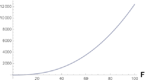
Figure 2: The diagram depicts the numerator (inside the brackets) of (3.35). It is positive, and hence the right-hand side of (3.35) as a whole is negative. Here, the horizontal axis is F$=-v(u+1)/3\epsilon$.

Similarly, we check that the QFC is satisfied in the case of no-island. We find

$$\partial_{v}\left(\dfrac{e^{-2\rho}}{\Omega}\right)\partial_{v}S^{\text{no-island}}_{\text{gen}}=-\dfrac{c}{24}\frac{(u+1)^{2}}{[1-v(u+1)]^{2}}\log\{M[1-v(u+1)]-1\}\,.$$ (3.36)

We can also calculate $\partial_{v}^{2}S^{\text{no-island}}_{\text{gen}}$ as

$$\partial_{v}^{2}S^{\text{no-island}}_{\text{gen}}= -\dfrac{c}{6}\dfrac{1}{v^{2}}\dfrac{1}{\log\left(\dfrac{v}{v_{0}}\right)}-\dfrac{c}{6}\dfrac{1}{v^{2}}\dfrac{1}{\left\{\log\left(\dfrac{v}{v_{0}}\right)\right\}^{2}}$$

$$+\dfrac{c}{12}\left\{\dfrac{u+1}{[1-v(u+1)]}\right\}^{2}-\dfrac{c}{24}\dfrac{1}{v^{2}}\,.$$ (3.37)

Therefore,

$$\partial_{v}\left(\dfrac{e^{-2\rho}}{\Omega}\right)\partial_{v}S^{\text{no-island}}_{\text{gen}}+\partial_{v}^{2}S^{\text{no-island}}_{\text{gen}}$$

$$=-\frac{c}{24}\dfrac{1}{v^{2}[1-v(u+1)]^{2}[\log(-\dfrac{v}{v_{0}})]^{2}}\cdot$$

$$\quad\times\Bigg{[}[1-v(u+1)]^{2}\left\{2+\log\left(\dfrac{v}{v_{0}}\right)\right\}^{2}$$

$$\qquad\quad+\left[\log\left(\dfrac{v}{v_{0}}\right)\right]^{2}(1+u)^{2}v^{2}\left\{\log[M(1-v(u+1)]-3\right\}\Bigg{]}\,.$$ (3.38)

This has much the same form as in the case of island. By the same argument before, we find that the right-hand side of (3.38) is negative. Thus, the QFC is satisfied.

3.3 Case (iii): $-v_{A}(1+u_{A})\sim\epsilon$

Finally, we discuss the case $-v_{A}(1+u_{A})\sim\epsilon$, in which $v_{A}$ and $v_{I}$ are very close. In this case, the assumption $\log(v_{A}/{v_{I}})\gg 1$ no longer holds, and the approximation used in (2.51) cannot be applied. Although the position of (the boundary of) the island is determined so that the generalized entropy is extremized, we do not substitute the position explicitly but treat $u_{I}$ and $v_{I}$ as functions of $u_{A}$ and $v_{A}$.

3.3.1 GSL

We calculate $\partial_{{v}_{A}}S_{\text{gen}}^{\text{island}}$ using generalized entropy (3.10).

$$\partial_{{v}_{A}}S_{\text{gen}}^{\text{island}}=\dfrac{c}{6v_{A}}\dfrac{1}{\log\left(\dfrac{v_{A}}{v_{I}}\right)}+\dfrac{c}{12}\dfrac{1+u_{A}}{\left[1-v_{A}(1+u_{A})\right]}-2M(1+u_{A})+\dfrac{c}{24}\dfrac{1}{v_{A}}\,.$$ (3.39)

By the same argument before, we find that the right-hand side of (3.39) is positive-definite, and therefore that $S_{\text{gen}}^{\text{island}}$ is non-decreasing.

3.3.2 GFC

To see whether QFC holds, we consider the following second-order derivative,

$$\partial_{v_{A}}\left(\dfrac{e^{-2\rho}}{\Omega}\partial_{v_{A}}S^{\text{island}}_{\text{gen}}\right)$$

$$=\dfrac{\partial}{\partial v_{A}}\left(\dfrac{e^{-2\rho}}{\Omega}\partial_{v_{A}}S^{\text{island}}_{\text{gen}}\right)+\dfrac{\partial v_{I}}{\partial v_{A}}\dfrac{\partial}{\partial v_{I}}\left(\dfrac{e^{-2\rho}}{\Omega}\partial_{v_{A}}S^{\text{island}}_{\text{gen}}\right)+\dfrac{\partial u_{I}}{\partial v_{A}}\dfrac{\partial}{\partial u_{I}}\left(\dfrac{e^{-2\rho}}{\Omega}\partial_{v_{A}}S^{\text{island}}_{\text{gen}}\right),$$

$$=\dfrac{\partial}{\partial v_{A}}\left(\dfrac{e^{-2\rho}}{\Omega}\partial_{v_{A}}S^{\text{island}}_{\text{gen}}\right)+\dfrac{\partial v_{I}}{\partial v_{A}}\dfrac{c}{6v_{A}v_{I}\left(\log\dfrac{v_{A}}{v_{I}}\right)^{2}}\,,$$ (3.40)

where the position of (the boundary of) the island $(u_{I},v_{I})$ depends on the position of the anchor point $(u_{A},v_{A})$. The partial derivative $\partial_{v_{A}}$ in the first line includes the variation of $v_{A}$ in $u_{I}(u_{A},v_{A})$ and $v_{I}(u_{A},v_{A})$, while those in the second and third line $\partial/\partial v_{A}$ is for fixed $(u_{I},v_{I})$. The third term in the second line is calculated to be zero. The first term in the third line is found to be negative by the same calculation as before. Therefore, in order for QFC to hold, $\partial v_{I}/\partial v_{A}$ must be negative.

Let us check whether $\partial v_{I}/\partial v_{A}$ is negative. First we note that eqs. (2.48) and (2.49) are rewritten as,

$$0 =-2M(1+u_{I})+\dfrac{c}{12}\frac{1+u_{I}}{1-v_{I}(1+u_{I})}+\dfrac{c}{24v_{I}}-\dfrac{c}{6v_{I}{\log\left(\dfrac{v_{A}}{v_{I}}\right)}}\,,$$ (3.41)

$$0 =-2Mv_{I}+\dfrac{c}{12}\dfrac{v_{I}}{1-v_{I}(1+u_{I})}+\dfrac{c}{24u_{I}}-\dfrac{c}{6u_{I}\log\left(\dfrac{u_{A}}{u_{I}}\right)}\,.$$ (3.42)

Noting that $v_{I}\gg 1,u_{I}\sim-1$, from eqs. (3.41) and (3.42), we obtain

$$0 \simeq\dfrac{c}{-12Mv_{I}(1+u_{I})+{c}/{4}}+\log\dfrac{v_{A}}{v_{I}}\,,$$ (3.43)

$$0 \simeq-\dfrac{c}{12Mv_{I}}+(u_{I}-v_{A})\,.$$ (3.44)

Taking ${v_{A}}$-derivatives of (3.43) and (3.44), we have respectively

$$0 =\frac{d}{dv_{A}}\frac{\partial S}{\partial v_{I}}$$

$$=\frac{1}{v_{A}}-\frac{\partial v_{I}}{\partial v_{A}}\left[\dfrac{12Mc(1+u_{I})}{\left\{-12Mv_{I}(1+u_{I})+{c}/{4}\right\}^{2}}+\dfrac{1}{v_{I}}\right]-\dfrac{\partial u_{I}}{\partial v_{A}}\dfrac{12Mcv_{I}}{\left\{-12Mv_{I}(1+u_{I})+{c}/{4}\right\}^{2}}\,,$$ (3.45)

$$0 =\dfrac{d}{dv_{A}}\dfrac{\partial S}{\partial u_{I}}=\dfrac{\partial v_{I}}{\partial v_{A}}\dfrac{c}{12Mv_{I}^{2}}+\dfrac{\partial u_{I}}{\partial v_{A}}\,.$$ (3.46)

From (3.45) and (3.46), we obtain

$$0 =\dfrac{\left\{-12Mv_{I}(1+u_{I})+{c}/{4}\right\}^{2}}{12Mcv_{I}v_{A}}-\dfrac{\partial v_{I}}{\partial v_{A}}\left[\frac{1+u_{I}}{v_{I}}+\dfrac{\left\{-12Mv_{I}(1+u_{I})+{c}/{4}\right\}^{2}}{12Mcv_{I}^{2}}-\dfrac{c}{12Mv_{I}^{2}}\right]$$

$$\equiv A-\frac{\partial v_{I}}{\partial v_{A}}B\,.$$ (3.47)

As mentioned below eq. (3.40), in order for QFC to hold, $\partial v_{I}/\partial v_{A}$ needs to be negative. Now we will show that $B$ is negative, as $A$ is obviously positive. $B$ is written as,

$$B=\frac{\left\{12Mv_{I}(1+u_{I})\right\}^{2}+6Mcv_{I}(1+u_{I})-{15c^{2}}/{16}}{12Mcv_{I}^{2}}\,.$$ (3.48)

Defining $X={12M}v_{I}(1+u_{I})/c$, we can express the numerator of (3.48) as $X^{2}+X/2-{15}/{16}$. Thus, the numerator of (3.48) vanishes when $X=-5/4,3/4$, and $B$ is negative for $-5/4<X<3/4$.

Now, we will show that an island exists only for $-5/4<X<3/4$. The position of (the boundary of) the island is determined by (3.43)–(3.44). Note that (3.44) can be transformed as follows:

$$u_{I}=\frac{c}{12Mv_{I}}+u_{A}\,.$$ (3.49)

We substitute this in (3.43) and obtain

$$\dfrac{c}{{12Mv_{I}}(1+u_{A})+{3c}/{4}}-\log v_{I}=-\log v_{A}\,.$$ (3.50)

Since $v_{A}\gg 1$, the right-hand side is negative. Eq. (3.50) has two solutions for sufficiently large $v_{A}$, but has no solution if $v_{A}$ is too small (see Figure 3). In $v_{A}\to\infty$, two solutions are $v_{I}\simeq-{3\epsilon}/({u_{A}+1})$ and $v_{I}\simeq v_{A}$. The former is the position of the island, which we have seen in the previous section, (2.52), and the latter gives a larger value of the generalized entropy, which is a false saddle point. Two solutions approach each other as $v_{A}$ is lowered, and eventually merges at some critical point, where the derivative of (3.50) vanishes.

Taking the derivative of (3.50) with respect to $v_{I}$ and then multiplying by $v_{I}$ we obtain

$$\left\{\frac{12Mv_{I}}{c}(1+u_{A})+\frac{3}{4}\right\}^{2}+\frac{12M}{c}v_{I}(1+u_{A})=0.$$ (3.51)

Defining $\tilde{X}={12M}v_{I}(1+u_{A})/c$, we can express the above equation (3.51) as $\tilde{X}+(\tilde{X}+{3}/{4})^{2}=0$. Thus, the solutions to (3.51) are $\tilde{X}=-1/4,-9/4$. This implies that two solutions of (3.50) are located in $\tilde{X}<-9/4$ and $-9/4<\tilde{X}<-3/4$, respectively. The solution in $-9/4<\tilde{X}<-3/4$ gives the position of the island and that in $\tilde{X}<-9/4$ is the false saddle. Note that $\tilde{X}=X+1$ and therefore an island exists when $-9/4<\tilde{X}<-3/4$, that is when $-5/4<X<1/4$. As seen above, when $-5/4<X<3/4$, $\partial v_{I}/\partial v_{A}<0$, and therefore

$$\frac{d\Theta}{d\lambda}<0.$$ (3.52)

Thus, the QFC is satisfied.

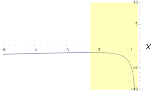
Figure 3: This figure depicts the solution of eq. (3.50). The vertical axis is $-\log v_{A}$ and the horizontal axis ${\tilde{X}}=12Mv_{I}(1+u_{A})/c$. From eq. (3.50), one finds that an island solution exists in the yellow region, where $-9/4<{\tilde{X}}<-3/4$.

4 Conclusion

In this paper, we have shown that the QFC holds for a two-dimensional evaporating black hole in RST model, with quantum backreaction on the geometry as well as the island formation taken into account. We have given a suitable definition of the quantum expansion in two-dimensions. The generalized entropy $S_{\text{gen}}$ is defined by the sum of the area entropy and the entropy of matter fields. In two dimensions, a Cauchy surface is separated by a point, and hence there is no notion of the area of that point. We treated $\Omega$ as the area entropy as in the previous studies on the RST model. In this paper, we showed that the generalized entropy is non-decreasing along outgoing null lines, even if the island affects the entropy of matter fields. We defined the quantum expansion (3.9), $\Theta=\dfrac{1}{2\Omega}\dfrac{dS_{\text{gen}}}{d\lambda}$, as the quantum expansion is defined as a variation of the generalized entropy per unit volume. Then, the QFC with our definition of the quantum expansion is satisfied for evaporating black holes in RST model, in both cases of the island configuration and no-island configuration.

In higher-dimensions, the QFC was used to derive the QNEC  [63, 64, 65]. In the two dimensional case, since the generalized entropy is given in terms of $\Omega$ as:

$$S_{\text{gen}}=2\Omega+S_{\rm out}\,,$$ (4.1)

where $S_{\text{out}}$ may be holographically given by $S_{\text{bulk}}$ in (2.43), it immediately follows from our definitions (3.6) and (3.9) that

$$\Theta=\theta+\dfrac{1}{2\Omega}\dfrac{dS_{\text{out}}}{d\lambda}\,.$$ (4.2)

When $\theta=0$, eq. (3.7) reduces to

$$\frac{d\theta}{d\lambda}=-\frac{e^{-4\rho}}{2\Omega}T_{++}\ ,$$ (4.3)

where $T_{++}$ is the energy-momentum tensor in the RST model (2.35). Then, our QFC implies, for $\theta=0$,

$$e^{-4\rho}T_{++}\geq\dfrac{d^{2}S_{\text{out}}}{d\lambda^{2}}\,.$$ (4.4)

This corresponds to the QNEC in two dimensions. In higher dimensions, the QNEC fails for some cases of interest [70, 71]. It would be interesting to clarify whether (under what circumstances) the QNEC may possibly fail in two dimensions.

Acknowledgments

This work was supported in part by JSPS KAKENHI Grant No. JP20K03930, JP20K03938 and also supported by MEXT KAKENHI Grant-in-Aid for Transformative Research Areas A Extreme Universe No. JP21H05182, JP21H05186.

References

- [1] R. Penrose, Phys. Rev. Lett. 14 (1965), 57-59 doi:10.1103/PhysRevLett.14.57
- [2] A. Borde, Class. Quant. Grav. 4, 343-356 (1987) doi:10.1088/0264-9381/4/2/015
- [3] G. Klinkhammer, Phys. Rev. D 43, 2542-2548 (1991) doi:10.1103/PhysRevD.43.2542
- [4] R. M. Wald and U. Yurtsever, Phys. Rev. D 44, 403-416 (1991) doi:10.1103/PhysRevD.44.403
- [5] L. H. Ford and T. A. Roman, Phys. Rev. D 51, 4277-4286 (1995) doi:10.1103/PhysRevD.51.4277 [arXiv:gr-qc/9410043 [gr-qc]].
- [6] N. Graham and K. D. Olum, Phys. Rev. D 76, 064001 (2007) doi:10.1103/PhysRevD.76.064001 [arXiv:0705.3193 [gr-qc]].
- [7] E. E. Flanagan and R. M. Wald, Phys. Rev. D 54, 6233-6283 (1996) doi:10.1103/PhysRevD.54.6233 [arXiv:gr-qc/9602052 [gr-qc]].
- [8] W. R. Kelly and A. C. Wall, Phys. Rev. D 90, no.10, 106003 (2014) [erratum: Phys. Rev. D 91, no.6, 069902 (2015)] doi:10.1103/PhysRevD.90.106003 [arXiv:1408.3566 [gr-qc]].
- [9] T. Faulkner, R. G. Leigh, O. Parrikar and H. Wang, JHEP 09, 038 (2016) doi:10.1007/JHEP09(2016)038 [arXiv:1605.08072 [hep-th]].
- [10] T. Hartman, S. Kundu and A. Tajdini, JHEP 07, 066 (2017) doi:10.1007/JHEP07(2017)066 [arXiv:1610.05308 [hep-th]].
- [11] D. Urban and K. D. Olum, Phys. Rev. D 81, 024039 (2010) doi:10.1103/PhysRevD.81.024039 [arXiv:0910.5925 [gr-qc]].
- [12] M. Visser, Phys. Lett. B 349, 443-447 (1995) doi:10.1016/0370-2693(95)00303-3 [arXiv:gr-qc/9409043 [gr-qc]].
- [13] A. Ishibashi, K. Maeda and E. Mefford, Phys. Rev. D 100, no.6, 066008 (2019) doi:10.1103/PhysRevD.100.066008 [arXiv:1903.11806 [hep-th]].
- [14] N. Iizuka, A. Ishibashi and K. Maeda, JHEP 03, 161 (2020) doi:10.1007/JHEP03(2020)161 [arXiv:1911.02654 [hep-th]].
- [15] F. Rosso, JHEP 07, 023 (2020) doi:10.1007/JHEP07(2020)023 [arXiv:2005.06476 [hep-th]].
- [16] N. Iizuka, A. Ishibashi and K. Maeda, JHEP 10, 106 (2020) doi:10.1007/JHEP10(2020)106 [arXiv:2008.07942 [hep-th]].
- [17] A. Ishibashi and K. Maeda, JHEP 03, 104 (2022) doi:10.1007/JHEP03(2022)104 [arXiv:2111.05151 [hep-th]].
- [18] J. D. Bekenstein, Lett. Nuovo Cim. 4 (1972), 737-740 doi:10.1007/BF02757029
- [19] J. D. Bekenstein, Phys. Rev. D 7 (1973), 2333-2346 doi:10.1103/PhysRevD.7.2333
- [20] R. Bousso, Z. Fisher, S. Leichenauer and A. C. Wall, Phys. Rev. D 93 (2016) no.6, 064044 doi:10.1103/PhysRevD.93.064044 [arXiv:1506.02669 [hep-th]].
- [21] G. Penington, JHEP 09 (2020), 002 doi:10.1007/JHEP09(2020)002 [arXiv:1905.08255 [hep-th]].
- [22] A. Almheiri, N. Engelhardt, D. Marolf and H. Maxfield, JHEP 12 (2019), 063 doi:10.1007/JHEP12(2019)063 [arXiv:1905.08762 [hep-th]].
- [23] A. Almheiri, R. Mahajan, J. Maldacena and Y. Zhao, JHEP 03 (2020), 149 doi:10.1007/JHEP03(2020)149 [arXiv:1908.10996 [hep-th]].
- [24] A. Almheiri, R. Mahajan and J. Maldacena, [arXiv:1910.11077 [hep-th]].
- [25] G. Penington, S. H. Shenker, D. Stanford and Z. Yang, JHEP 03 (2022), 205 doi:10.1007/JHEP03(2022)205 [arXiv:1911.11977 [hep-th]].
- [26] A. Almheiri, T. Hartman, J. Maldacena, E. Shaghoulian and A. Tajdini, JHEP 05 (2020), 013 doi:10.1007/JHEP05(2020)013 [arXiv:1911.12333 [hep-th]].
- [27] D. N. Page, Phys. Rev. Lett. 71 (1993), 3743-3746 doi:10.1103/PhysRevLett.71.3743 [arXiv:hep-th/9306083 [hep-th]].
- [28] D. N. Page, JCAP 09 (2013), 028 doi:10.1088/1475-7516/2013/09/028 [arXiv:1301.4995 [hep-th]].
- [29] H. Z. Chen, Z. Fisher, J. Hernandez, R. C. Myers and S. M. Ruan, JHEP 03, 152 (2020) doi:10.1007/JHEP03(2020)152 [arXiv:1911.03402 [hep-th]].
- [30] A. Almheiri, R. Mahajan and J. E. Santos, SciPost Phys. 9, no.1, 001 (2020) doi:10.21468/SciPostPhys.9.1.001 [arXiv:1911.09666 [hep-th]].
- [31] D. Marolf and H. Maxfield, JHEP 08, 044 (2020) doi:10.1007/JHEP08(2020)044 [arXiv:2002.08950 [hep-th]].
- [32] V. Balasubramanian, A. Kar, O. Parrikar, G. Sárosi and T. Ugajin, JHEP 01, 177 (2021) doi:10.1007/JHEP01(2021)177 [arXiv:2003.05448 [hep-th]].
- [33] F. F. Gautason, L. Schneiderbauer, W. Sybesma and L. Thorlacius, JHEP 05, 091 (2020) doi:10.1007/JHEP05(2020)091 [arXiv:2004.00598 [hep-th]].
- [34] T. Anegawa and N. Iizuka, JHEP 07, 036 (2020) doi:10.1007/JHEP07(2020)036 [arXiv:2004.01601 [hep-th]].
- [35] K. Hashimoto, N. Iizuka and Y. Matsuo, JHEP 06, 085 (2020) doi:10.1007/JHEP06(2020)085 [arXiv:2004.05863 [hep-th]].
- [36] J. Sully, M. Van Raamsdonk and D. Wakeham, JHEP 03, 167 (2021) doi:10.1007/JHEP03(2021)167 [arXiv:2004.13088 [hep-th]].
- [37] T. Hartman, E. Shaghoulian and A. Strominger, JHEP 07, 022 (2020) doi:10.1007/JHEP07(2020)022 [arXiv:2004.13857 [hep-th]].
- [38] T. J. Hollowood and S. P. Kumar, JHEP 08, 094 (2020) doi:10.1007/JHEP08(2020)094 [arXiv:2004.14944 [hep-th]].
- [39] C. Krishnan, V. Patil and J. Pereira, [arXiv:2005.02993 [hep-th]].
- [40] M. Alishahiha, A. Faraji Astaneh and A. Naseh, JHEP 02, 035 (2021) doi:10.1007/JHEP02(2021)035 [arXiv:2005.08715 [hep-th]].
- [41] H. Z. Chen, R. C. Myers, D. Neuenfeld, I. A. Reyes and J. Sandor, JHEP 10, 166 (2020) doi:10.1007/JHEP10(2020)166 [arXiv:2006.04851 [hep-th]].
- [42] A. Almheiri, T. Hartman, J. Maldacena, E. Shaghoulian and A. Tajdini, Rev. Mod. Phys. 93, no.3, 035002 (2021) doi:10.1103/RevModPhys.93.035002 [arXiv:2006.06872 [hep-th]].
- [43] H. Geng and A. Karch, JHEP 09, 121 (2020) doi:10.1007/JHEP09(2020)121 [arXiv:2006.02438 [hep-th]].
- [44] R. Bousso and E. Wildenhain, Phys. Rev. D 102, no.6, 066005 (2020) doi:10.1103/PhysRevD.102.066005 [arXiv:2006.16289 [hep-th]].
- [45] C. Krishnan, JHEP 01, 179 (2021) doi:10.1007/JHEP01(2021)179 [arXiv:2007.06551 [hep-th]].
- [46] Y. Chen, V. Gorbenko and J. Maldacena, JHEP 02, 009 (2021) doi:10.1007/JHEP02(2021)009 [arXiv:2007.16091 [hep-th]].
- [47] T. Hartman, Y. Jiang and E. Shaghoulian, JHEP 11, 111 (2020) doi:10.1007/JHEP11(2020)111 [arXiv:2008.01022 [hep-th]].
- [48] V. Balasubramanian, A. Kar and T. Ugajin, JHEP 02, 072 (2021) doi:10.1007/JHEP02(2021)072 [arXiv:2008.05275 [hep-th]].
- [49] H. Z. Chen, R. C. Myers, D. Neuenfeld, I. A. Reyes and J. Sandor, JHEP 12, 025 (2020) doi:10.1007/JHEP12(2020)025 [arXiv:2010.00018 [hep-th]].
- [50] J. Hernandez, R. C. Myers and S. M. Ruan, JHEP 02, 173 (2021) doi:10.1007/JHEP02(2021)173 [arXiv:2010.16398 [hep-th]].
- [51] H. Geng, A. Karch, C. Perez-Pardavila, S. Raju, L. Randall, M. Riojas and S. Shashi, SciPost Phys. 10, no.5, 103 (2021) doi:10.21468/SciPostPhys.10.5.103 [arXiv:2012.04671 [hep-th]].
- [52] H. Geng, Y. Nomura and H. Y. Sun, Phys. Rev. D 103, no.12, 126004 (2021) doi:10.1103/PhysRevD.103.126004 [arXiv:2103.07477 [hep-th]].
- [53] H. Geng, A. Karch, C. Perez-Pardavila, S. Raju, L. Randall, M. Riojas and S. Shashi, JHEP 01, 182 (2022) doi:10.1007/JHEP01(2022)182 [arXiv:2107.03390 [hep-th]].
- [54] Y. Matsuo, JHEP 12 (2023), 050 doi:10.1007/JHEP12(2023)050 [arXiv:2308.05009 [hep-th]].
- [55] E. Witten, Phys. Rev. D 44 (1991), 314-324 doi:10.1103/PhysRevD.44.314
- [56] S. Elitzur, A. Forge and E. Rabinovici, Nucl. Phys. B 359 (1991), 581-610 doi:10.1016/0550-3213(91)90073-7
- [57] G. Mandal, A. M. Sengupta and S. R. Wadia, Mod. Phys. Lett. A 6 (1991), 1685-1692 doi:10.1142/S0217732391001822
- [58] R. Dijkgraaf, H. L. Verlinde and E. P. Verlinde, Nucl. Phys. B 371 (1992), 269-314 doi:10.1016/0550-3213(92)90237-6
- [59] C. G. Callan, Jr., S. B. Giddings, J. A. Harvey and A. Strominger, Phys. Rev. D 45 (1992) no.4, R1005 doi:10.1103/PhysRevD.45.R1005 [arXiv:hep-th/9111056 [hep-th]].
- [60] J. G. Russo, L. Susskind and L. Thorlacius, Phys. Rev. D 46 (1992), 3444-3449 doi:10.1103/PhysRevD.46.3444 [arXiv:hep-th/9206070 [hep-th]].
- [61] A. Bilal and C. G. Callan, Jr., Nucl. Phys. B 394 (1993), 73-100 doi:10.1016/0550-3213(93)90102-U [arXiv:hep-th/9205089 [hep-th]].
- [62] V. P. Frolov, Phys. Rev. D 46, 5383-5394 (1992) doi:10.1103/PhysRevD.46.5383
- [63] R. Bousso, Z. Fisher, J. Koeller, S. Leichenauer and A. C. Wall, Phys. Rev. D 93, no.2, 024017 (2016) doi:10.1103/PhysRevD.93.024017 [arXiv:1509.02542 [hep-th]].
- [64] J. Koeller and S. Leichenauer, Phys. Rev. D 94, no.2, 024026 (2016) doi:10.1103/PhysRevD.94.024026 [arXiv:1512.06109 [hep-th]].
- [65] Z. Fu, J. Koeller and D. Marolf, Class. Quant. Grav. 34, no.22, 225012 (2017) [erratum: Class. Quant. Grav. 35, no.4, 049501 (2018)] doi:10.1088/1361-6382/aa8f2c [arXiv:1706.01572 [hep-th]].
- [66] R. M. Wald, Phys. Rev. D 48, no.8, R3427-R3431 (1993) doi:10.1103/PhysRevD.48.R3427 [arXiv:gr-qc/9307038 [gr-qc]].
- [67] R. C. Myers, Phys. Rev. D 50, 6412-6421 (1994) doi:10.1103/PhysRevD.50.6412 [arXiv:hep-th/9405162 [hep-th]].
- [68] R. Emparan, D. Grumiller and K. Tanabe, Phys. Rev. Lett. 110, no.25, 251102 (2013) doi:10.1103/PhysRevLett.110.251102 [arXiv:1303.1995 [hep-th]].
- [69] J. Soda, Prog. Theor. Phys. 89, 1303-1310 (1993) doi:10.1143/PTP.89.1303
- [70] Z. Fu, J. Koeller and D. Marolf, Class. Quant. Grav. 34, no.17, 175006 (2017) doi:10.1088/1361-6382/aa80ba [arXiv:1705.03161 [hep-th]].
- [71] A. Ishibashi, K. Maeda and E. Mefford, Phys. Rev. D 99, no.2, 026004 (2019) doi:10.1103/PhysRevD.99.026004 [arXiv:1808.05192 [hep-th]].