\tnotetext

[1]K. V. M. acknowledges support from the National Academies of Sciences, Engineering, and Medicine via the Army Research Laboratory Harry Diamond Distinguished Fellowship. The following co-authors are a member of EURASIP: Kumar Vijay Mishra.

[orcid=0000-0002-5386-609X]

label1]organization=The University of Texas at Dallas, city=Richardson, postcode=TX 75080, country=USA label2]organization=United States DEVCOM Army Research Laboratory, city=Adelphi, postcode=MD 20783, country=USA

Co-Designing Statistical MIMO Radar and In-band Full-Duplex Multi-User MIMO Communications – Part III: Multi-Target Tracking

Sk Nayemuzzaman    Kumar Vijay Mishra    Jiawei Liu    Mohammad Saquib [ [
Abstract

As a next-generation wireless technology, the in-band full-duplex (IBFD) transmission enables simultaneous transmission and reception of signals over the same frequency, thereby doubling spectral efficiency. Further, a continuous up-scaling of wireless network carrier frequencies arising from ever-increasing data traffic is driving research on integrated sensing and communications (ISAC) systems. In this context, we study the co-design of common waveforms, precoders, and filters for an IBFD multi-user (MU) multiple-input multiple-output (MIMO) communications with a distributed MIMO radar. This paper, along with companion papers (Part I and II), proposes a comprehensive MRMC framework that addresses all these challenges. In the companion papers, we developed signal processing and joint design algorithms for this distributed system. In this paper, we tackle multi-target detection, localization, and tracking. This co-design problem that includes practical MU-MIMO constraints on power and quality-of-service is highly non-convex. We propose a low-complexity procedure based on Barzilai–Borwein gradient algorithm to obtain the design parameters and mixed-integer linear program for distributed target localization. Numerical experiments demonstrate the feasibility and accuracy of multi-target sensing of the distributed FD ISAC system. Finally, we localize and track multiple targets by adapting the joint probabilistic data association and extended Kalman filter for this system.

1 Introduction

Conventional communications systems are based on either half-duplex (HD) or out-of-band full-duplex (FD) transmission for low-complexity transceiver designs. In such systems, uplink (UL) and downlink (DL) communications are separated in either time or frequency through, for example, time- or frequency-division duplexing, respectively, leading to reduced spectral efficiency [1, 2]. Recently, in response to a tremendous rise in wireless data traffic, in-band full-duplex (IBFD) operation has been suggested as a promising technology to increase spectral efficiency. The IBFD enables concurrent transmission and reception in a single time/frequency channel to potentially double the attainable spectral efficiency and throughput and reduce latency [3]. Recent breakthroughs in SI cancellation (SIC) techniques at both radio-frequency and baseband stages enable an SI suppression of more than $100$ dB and are critical to the more rapid deployment of IBFD-enabled transceivers [1]. The MIMO evolution of 3GPP Release 18 [4] aggregates two HD sub-bands into a sub-band FD in its schedule.

One of the promising IBFD applications is the emerging area of integrated sensing and communications (ISAC), wherein radar and communications functions concurrently operate in the same spectral range to address the severe spectral crowding problem [5, 6, 7]. For example, with FD, the base station (BS) is able to receive DL echo signals and estimate radar target parameters. Furthermore, FD allows for the use of joint optimization methods to make a good trade-off. The joint FD ISAC design has the potential for greater spectral efficiency, hardware sharing, and system integration [8, 9, 10, 1, 11, 12].

More recently, the ISAC systems with MIMO radars and MIMO communications (MRMC) have received much attention because, individually, both systems are designed for efficient spectrum usage due to increased degrees-of-freedom in the spatial domain [13, 14, 15]. The MIMO radars are usually classified as colocated [16, 17] and widely distributed/statistical [18] depending on the geometry of antenna placement. In a colocated MIMO radar [19], the radar cross-section (RCS) is identical to closely-spaced antennas. But, in a distributed MIMO radar, antennas are sufficiently separated and isotropic so that the same target appears with a different RCS to each transmit-receive antenna pair [20]. The MRMC literature has largely focused on co-located MIMO radar [18, 21]. In the first companion paper (Part I) [22], we proposed spectral co-design of statistical MIMO radar with IBFD MU-MIMO communications. In the second companion paper (Part II) [23], we developed an algorithm that jointly designed the radar waveform code, communications precoders, and linear receive filters for this distributed system. In this paper, we consider distributed beamforming (DB) and multi-target tracking for the same framework.

In wireless sensor networks, DB is employed to achieve the desired signal-to-noise (SNR) and reduce power assumption by providing a coherent beamforming gain [24, 25, 26, 27, 28, 29]. It is cooperative communications in which distributed transmitters adjust the phases of their signals in a way that the signals are constructively combined at a client [27]. Some studies also use this term for beamforming algorithm that is solved in a distributed manner where each user only relies on local information to perform beamforming [30, 31]. The coherent combination of various waveforms is accomplished through appropriate synchronization between transmitters [32]. As a mechanism for cooperative communications, distributed transmit beamforming enables a group of individual source user equipment (UE) to transmit a common message signal as a virtual antenna array such that the bandpass transmissions aggregate constructively after propagation at an intended destination [29].

Compared to conventional beamforming [33, 34, 35], the DB relies on each sensor to derive its carrier signal from a separate local oscillator. The independent local oscillator at each UE has random initial phase and phase noise, which forbid phase alignment of signals from different transmitters (Txs) at the receivers (Rxs) of destination UEs [26, 24]. Distributed co-phasing (DCP) is one of the promising techniques to achieve distributed transmit beamforming by combining the coherent gain with the spatial diversity gain. This technique offers benefits such as fixed power transmission from the UEs, robustness to channel estimation errors, and feasibility for practical implementations [36, 29]. In essence, DCP employs the multiple transmitting nodes as a distributed antenna array to achieve coherent combining gain as well as diversity gain for wireless sensors network [37].

The DB technique has also been explored for multiple-input multiple-output (MIMO) radars in the form of distributed coherent systems, wherein accurate phase synchronization is required to obtain coherent processing gain [38, 39]. Based on the antenna placement relative to the target cross-section (RCS), MIMO radars may be colocated (target RCS appears identical to all Tx-Rx pairs) [19, 40, 41, 42] or distributed (where the Tx and Rx antennas are widely separated and RCS is different for each Tx-Rx pair) [43, 44, 18]. Distributed MIMO radars may be non-coherent or coherent, depending on whether the phase information is ignored or included [45]. The former extracts diversity gains across different Tx-Rx pairs to overcome target RCS fading, while the latter requires accurate Tx-Rx phase synchronization to exploit processing gains [38, 39]. Herein, we study the distributed coherent MIMO radar (MIMO radar) because these systems have improved direction finding accuracy over their non-coherent counterparts by ensuring phase coherence of carrier signals from different distributed radar elements [38].

In practice, the accuracy of the phase in the transmit time slot determines the achievable beamforming gain [24]. Therefore, within the realm of DB, considerable efforts have been dedicated to either the carrier frequency/phase synchronization protocol establishment [25, 38, 46] or error analysis when mismatched phases occur [26, 39, 29]. Master-slave  [46], round trip [25] and broadcast consensus algorithms [38] are efficient approaches to achieving phase synchronization in a distributed system. The probability of outage with imperfect channel state information (CSI) has also been studied for a distributed wireless sensor network such as cloud radio access network (C-RAN) [29]. More recently, distributed co-phasing, which combines the coherent combining gain with the spatial diversity gain, has been proposed for C-RANs [47, 48]. This technique offers benefits such as fixed power transmission from the UEs, robustness to channel estimation errors, and feasibility for practical implementations [36].

Table 1: Comparison with the state-of-the-art
q.v. Radar Communications Design objective
Model Targets; Clutter Tracking Model Duplexing Users Beamformers
[13] C-MIMOa Static, single; Yes No P2P MIMOb HD SU Max-SINR Waveforms
[49] D-MIMOc Static, single; Yes No D-MIMO HD SU None Radar Rx filters
[50] Monostatic Static, multiple; Yes No M-MIMOd HD (UL) SU Zero Force Rx filters, BFs
[51] C-MIMO Static, single; No No MIMO HD (DL) MU C. I.e Transmit BFs
[14] C-MIMO Moving, single; No No MIMO FD MU NSP BFs, radar waveform
[31] C-MIMO Moving, single; No No MIMO FD MU Max-SNR BF
[52] Monostatic Moving, single; No No P2P SISO IBFD SU None Waveform
[22, 23] D-MIMO Moving, single; Yes No MIMO IBFD MU Max-MI Waveform, precoders, filter
This paper D-MIMO Moving, multiple; Yes Yes C-RAN MIMO IBFD MU Co-phased Max-MI Waveform, precoders, filter, power
  • a

    C-MIMO: Colocated MIMO

  • b

    P2P: Point-to-point

  • c

    D-MIMO: Distributed MIMO

  • d

    M-MIMO: Massive MIMO

  • e

    Constructive interference

Preliminary results of this work appeared in our conference publication [53], where only a few antenna geometries were considered, DCP was excluded, and optimization algorithm was not described. In this paper, we focus on ISAC design with distributed MIMO radar and IBFD C-RAN, employ co-phasing, use a unified design metric, propose a low-complexity design algorithm, and include multiple targets. Table 1 summarizes our contributions with respect to the state-of-the-art. Our main contributions are:
1) IBFD C-RAN: We consider a full duplex C-RAN (FD-C-RAN) where the RRHs are equipped with the IBFD technique and are able to communicate with DMUs and UMUs simultaneously. A typical C-RAN consists of a pool of baseband units (BBUs), a large number of remote radio heads (RRHs), and a Fronthaul network connecting RRHs to BBUs. The BBU pool is deployed at a centralized site, where software-defined BBUs process the baseband signals and coordinate the wireless resource allocation. The RRHs are in charge of RF amplification, up/down-conversion, filtering, analog-to-digital/digital-to-analog conversion, and interface adaption.
2) Low-complexity design algorithm: To this end, we employ an alternating minimization procedure, which includes low-complexity Barzilai-Borwein (BB) algorithm [54] for precoder design subproblem. The BB method is an efficient tool for solving large-scale unconstrained optimization problems. When compared to the steepest descent method, it has the same search direction but a different step rule. Our BB-based design achieves similar results as the more complex conventional approaches such as the block coordinate descent (BCD) [55].
3) Multiple targets: The presence of multiple targets in a distributed ISAC scenario poses additional challenges. Since the relative distance of each target is different with respect to each Rx, the echoes from multiple targets are delayed by a different amount at each Rx. The result is that, after the detection procedure, each Rx ends up with a different ordering of targets in time. This makes it difficult to associate the detected echoes from all Rx uniquely to each target [56, 57, 58, 59]. To this end, the distributed radar literature suggests various data association algorithms such as multiple hypothesis tracking [60], random finite sets [61], and joint probabilistic data association (JPDA) [62]. we propose JPDA to assign detections from both radar and DL signals to specific targets.

The remainder of the paper is organized as follows. The next section describes our FD-ISAC system and the stand-alone radar and communications receivers. In 3, we introduce FD D-ISAC receiver processing for self-interference, radar-to-communications interference, and vice versa. Section 4 presents our proposed multi-target CWSM optimization using the low-complexity BBB procedure. The multi-target detection via data association in D-ISAC is discussed in Section 5 followed by extensive numerical experiments in Section 6. We conclude in Section 7.

Throughout this paper, lowercase regular, lowercase boldface, and uppercase boldface letters denote scalars, vectors, and matrices, respectively. We use $I(\mathbf{X};\mathbf{Y})$ and $H\left({\mathbf{X}|\mathbf{Y}}\right)$ to denote MI and conditional entropy between two random variables $\mathbf{X}$ and $\mathbf{Y}$, respectively. The notations $\mathbf{Y}{\left[{k}\right]}$, $\mathbf{y}{\left[{k}\right]}$, and $y{\left[{k}\right]}$ denote the value of time-variant matrix $\mathbf{Y}$, vector $\mathbf{y}$ and scalar $y$ at discrete-time index $k$, respectively; $\mathbf{1}_{N}$ is a vector of size $N$ with all ones; $\mathbb{C}$ and $\mathbb{R}$ represent sets of complex and real numbers, respectively; a circularly symmetric complex Gaussian (CSCG) vector $\mathbf{q}$ with $N$ elements and power spectral density $\mathcal{N}_{0}$ is $\mathbf{q}\sim\mathcal{CN}(0,\mathcal{N}_{0}\mathbf{I}_{N})$; $(\cdot)^{\star}$ is the solution of the optimization problem; $\mathbb{E}{\left[{\cdot}\right]}$ is the statistical expectation; $\operatorname{tr}\{\mathbf{R}\}$, $\mathbf{R}^{\top}$, $\mathbf{R}^{\dagger}$, $\mathbf{R}^{\ast}$, $\left|\mathbf{R}\right|$, $\mathbf{R}\succeq\mathbf{0}$, and $\mathbf{R}\left({m,n}\right)$ are the trace, transpose, Hermitian transpose, element-wise complex conjugate, determinant, positive semi-definiteness and ${\left({m,n}\right)}^{\underline{\text{th}}}$ entry of matrix $\mathbf{R}$, respectively; set $\mathbb{Z}_{+}(L)$ denotes $\left\{1,\dots,L\right\}$; $\mathbf{x}\succeq\mathbf{y}$ denotes component-wise inequality between vectors $\mathbf{x}$ and $\mathbf{y}$; $x^{+}$ represents $\max(x,0)$; $x^{\left({t}\right)}\left({\cdot}\right)$ is the ${t}^{\underline{\text{th}}}$ iterate of an iterative function $x\left({\cdot}\right)$; $\inf(\cdot)$ is the infimum of its argument; $\odot$ denotes the Hadamard product; and $\oplus$ is the direct sum. All distances are measured in kilometers.

2 System Model

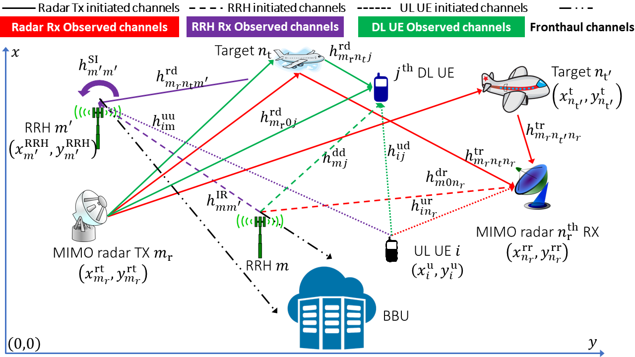
We consider an FD-ISAC system consisting of a MIMO radar with $M_{\mathrm{r}}$ ($N_{\mathrm{r}}$) widely distributed single antenna Txs (Rxs) and an FD C-RAN, which encompasses $N_{\mathrm{B}}$ FD RRHs jointly serving $\mathit{J}$ ($\mathit{I}$) single antenna HD DL (UL) UEs concurrently. Each FD RRH is equipped with $M_{\mathrm{c}}$ transceiving antennas and connected to the BBU via a fiber-fronthaul link. The MIMO radar detects and localizes $N_{\mathrm{t}}$ moving targets within the coverage of the FD-C-RAN during an ISAC operation window when the $M$ FD RRHs coherently broadcast data streams to each DL UE while the $I$ UL UEs multi-access channel to all RRUs. Simultaneously, each radar Tx emits a train of $\mathit{K}$ pulses to detect a moving target in the coverage area of the BS at a uniform pulse repetition interval (PRI) $T_{\mathrm{r}}$; the total duration $KT_{\mathrm{r}}$ is the coherent processing interval (CPI). The integration of FD communications and radar sensing allows the radar pulse width, PRI, and CPI to equal the communications symbol duration, frame length, and scheduling window, respectively. As a result, the number of symbol periods in each frame, $L$, equals the number of range bins. Figure 1 illustrates the system model on a two-dimensional (2-D) $\left(x\textrm{-}y\right)$ Cartesian plane $\left(x,y\right)$.

2.1 Transmit signal

For the FD-C-RAN, we adopt an all-RRH association policy, namely that all corresponding FD RRHs cooperatively transmit DL signals to each DL UE while each UL UE sends a common single-stream data symbol $M$ FD RRHs [63]. During the the ${l}^{\underline{\text{th}}}$ symbol period of the ${k}^{\underline{\text{th}}}$ frame or the ${{\left[{k,l}\right]}}^{\underline{\text{th}}}$ symbol period, of the ISAC operation window, FD RRH $m\in{\left\{{1,\cdots,M}\right\}}$ and UL UE $i\in{\left\{{1,\cdots,I}\right\}}$ simultaneously transmit DL and UL signals $x_{\mathrm{d},m}{\left[{k,l}\right]}=\sum_{j=1}^{J}\mathbf{v}_{\mathrm{d},mj}s_{\mathrm{d},j}{\left[{k,l}\right]}$ and $x_{\mathrm{u},i}{\left[{k,l}\right]}=\sqrt{P_{\mathrm{u},i}}s_{\mathrm{u},i}{\left[{k,l}\right]}$, respectively, where $\mathbf{v}^{\mathrm{d}}_{mj}\in\mathbb{C}^{M_{\mathrm{c}}}$ and $P_{\mathrm{u},i}$ are the DL beamforming vector and the transmit power employed by the ${m}^{\underline{\text{th}}}$ RRH towards the ${j}^{\underline{\text{th}}}$ DL UE and the ${i}^{\underline{\text{th}}}$ UL UE, respectively; $s_{\mathrm{d},j}{\left[{k,l}\right]}$ ($s_{\mathrm{u},i}{\left[{k,l}\right]}$) designates the single the data stream for the ${j}^{\underline{\text{th}}}$ DL (${i}^{\underline{\text{th}}}$ UL) UE with $\mathbb{E}{\left[{\lvert s_{\mathrm{d},j}{\left[{k,l}\right]}\rvert^{2}}\right]}=1$ ($\mathbb{E}{\left[{\lvert s_{\mathrm{u},i}{\left[{k,l}\right]}\rvert^{2}}\right]}=1$).

Denote the radar pulse duration as $T_{\mathrm{p}}=T_{\mathrm{r}}/N_{\mathrm{p}}$ (a.k.a fast time), where $N_{\mathrm{p}}$ is the number of range cells per PRI. We define the radar code vector transmitted during the ${k}^{\underline{\text{th}}}$ PRI as $\mathbf{a}{\left[{k}\right]}={\left[{a_{k,1},\cdots,a_{k,\mathit{M}_{\mathrm{r}}}}\right]}^{\top}\in\mathbb{C}^{M_{\mathrm{r}}}$ and the MIMO radar code matrix as $\mathbf{A}={\left[{\mathbf{a}{\left[{1}\right]},\cdots,\mathbf{a}{\left[{\mathrm{\mathit{K}}}\right]}}\right]}\in\mathbb{C}^{M_{\mathrm{r}}\times K}$. The pulse train transmitted by the ${m_{\mathrm{r}}}^{\underline{\text{th}}}$ radar Tx is written as $s_{m_{\mathrm{r}}}(t)=\sum_{k=0}^{K-1}a_{k,m_{\mathrm{r}}}\phi_{m_{\mathrm{r}}}\left({t-kT_{\mathrm{r}}}\right)$ $\mathit{K}$, where $\phi_{m_{\mathrm{r}}}(t)$ denotes the orthonormal waveform associated with the ${m_{\mathrm{r}}}^{\underline{\text{th}}}$ radar Tx with support $[0,T_{\mathrm{p}})$. Grouping the transmit signals from $M_{\mathrm{r}}$ Txs yields $\mathbf{s}(t)={\left[{s_{1}(t),\cdots,s_{M_{\mathrm{r}}}(t)}\right]}^{\top}$.

Refer to caption
Figure 1: Illustration of the considered D-ISAC system, where the ${m_{\mathrm{r}}}^{\underline{\text{th}}}$ (${n_{\mathrm{r}}}^{\underline{\text{th}}}$) radar Tx (Rx), ${m}^{\underline{\text{th}}}$ FD RRH, ${j}^{\underline{\text{th}}}$ (${i}^{\underline{\text{th}}}$) DL (UL) UE are located at $\left({x^{\mathrm{rt}}_{m_{\mathrm{r}}},y^{\mathrm{rt}}_{m_{\mathrm{r}}}}\right)$ ($\left({x^{\mathrm{rr}}_{n_{\mathrm{r}}},y^{\mathrm{rr}}_{n_{\mathrm{r}}}}\right)$), $\left({x^{\mathrm{RRH}}_{m},y^{\mathrm{RRH}}_{m}}\right)$, $\left({x^{\mathrm{d}}_{j},y_{\mathrm{d},j}}\right)$ ($\left({x_{\mathrm{u},i},y^{\mathrm{u}}_{i}}\right)$), respectively; the ${n_{\mathrm{t}}}^{\underline{\text{th}}}$ target is located at $\left({x_{\mathrm{t},n_{\mathrm{t}}},y_{\mathrm{t},n_{\mathrm{t}}}}\right)$.

2.2 Channel

During a given CPI, the ${n_{\mathrm{t}}}^{\underline{\text{th}}}$ moving target is located at $\left({x_{\mathrm{t},n_{\mathrm{t}}},y_{\mathrm{t},n_{\mathrm{t}}}}\right)$ with the horizontal and vertical velocity as $\left({\dot{x}_{\mathrm{t},n_{\mathrm{t}}},\dot{y}_{\mathrm{t},n_{\mathrm{t}}}}\right)$. Then we define the state vector of the ${n_{\mathrm{t}}}^{\underline{\text{th}}}$ target as $\mathbf{x}_{\mathrm{t},n_{\mathrm{t}}}={\left[{x_{\mathrm{t},n_{\mathrm{t}}},y_{\mathrm{t},n_{\mathrm{t}}},\dot{x}_{\mathrm{t},n_{\mathrm{t}}},\dot{y}_{\mathrm{t},n_{\mathrm{t}}}}\right]}^{\top}$ The propagation delay and Doppler shift associated with the ${\left({m_{\mathrm{r}}n_{\mathrm{t}}n_{\mathrm{r}}}\right)}^{\underline{\text{th}}}$ Tx-target-Rx path are observed as

$\displaystyle b_{\tau,m_{\mathrm{r}}n_{\mathrm{r}}}\left({\mathbf{x}_{\mathrm{t},n_{\mathrm{t}}}}\right)$ $\displaystyle\triangleq\tau_{m_{\mathrm{r}}n_{\mathrm{t}}n_{\mathrm{r}}}=\frac{r_{\mathrm{r},m_{\mathrm{r}}n_{\mathrm{t}}n_{\mathrm{r}}}}{c}=\frac{r_{m_{\mathrm{r}}n_{\mathrm{t}}m}+r_{n_{\mathrm{t}}n_{\mathrm{r}}}}{c}$ (1)
$\displaystyle b_{f,m_{\mathrm{r}}n_{\mathrm{r}}}\left({\mathbf{x}_{\mathrm{t},n_{\mathrm{t}}}}\right)$ $\displaystyle\triangleq f_{m_{\mathrm{r}}n_{\mathrm{t}}n_{\mathrm{r}}}$
$\displaystyle=\frac{\dot{x}_{\mathrm{t},n_{\mathrm{t}}}\left({x_{\mathrm{t},n_{\mathrm{t}}}-x_{\mathrm{tx},m_{\mathrm{r}}}}\right)+\dot{y}_{\mathrm{t},n_{\mathrm{t}}}\left({y_{\mathrm{t},n_{\mathrm{t}}}-y_{\mathrm{rt},m_{\mathrm{r}}}}\right)}{\lambda r_{m_{\mathrm{r}}n_{\mathrm{t}}m}}+\frac{\dot{x}_{\mathrm{t},n_{\mathrm{t}}}\left({x_{\mathrm{t},n_{\mathrm{t}}}-x^{\mathrm{rr}}_{n_{\mathrm{r}}}}\right)+\dot{y}_{\mathrm{t},n_{\mathrm{t}}}\left({y_{\mathrm{t},n_{\mathrm{t}}}-y^{\mathrm{rr}}_{n_{\mathrm{r}}}}\right)}{\lambda r_{n_{\mathrm{t}}n_{\mathrm{r}}}}$ (2)

where $b_{\tau,m_{\mathrm{r}}n_{\mathrm{r}}}\left({\cdot}\right)$ and $b_{f,m_{\mathrm{r}}n_{\mathrm{r}}}\left({\cdot}\right)$ are the delay and Doppler observation functions, $\lambda$ and $c$ denote the carrier wavelength and the speed of light, respectively; $r_{\mathrm{r},m_{\mathrm{r}}n_{\mathrm{t}}n_{\mathrm{r}}}$ represents the bistatic range between the ${m_{\mathrm{r}}}^{\underline{\text{th}}}$ radar Tx, ${n}^{\underline{\text{th}}}_{\mathrm{t}}$ target, and ${n_{\mathrm{r}}}^{\underline{\text{th}}}$ radar Rx with

$\displaystyle r_{m_{\mathrm{r}}n_{\mathrm{t}}m}=$ $\displaystyle\sqrt{\left({x_{\mathrm{t},n_{\mathrm{t}}}-x_{\mathrm{tx},m_{\mathrm{r}}}}\right)^{2}+\left({y_{\mathrm{t},n_{\mathrm{t}}}-y_{\mathrm{rt},m_{\mathrm{r}}}}\right)^{2}}$ (3)
$\displaystyle r_{n_{\mathrm{t}}n_{\mathrm{r}}}=$ $\displaystyle\sqrt{\left({x_{\mathrm{t},n_{\mathrm{t}}}-x^{\mathrm{rr}}_{n_{\mathrm{r}}}}\right)^{2}+\left({y_{\mathrm{t},n_{\mathrm{t}}}-y^{\mathrm{rr}}_{n_{\mathrm{r}}}}\right)^{2}}.$ (4)

We then write the composite channel coefficient between Tx $m_{\mathrm{r}}$, target $n_{\mathrm{t}}$, and Rx $n_{\mathrm{r}}$ as

$$h^{\mathrm{r}}_{m_{\mathrm{r}}n_{\mathrm{t}}n_{\mathrm{r}}}\triangleq r^{-2}_{\mathrm{r},m_{\mathrm{r}}n_{\mathrm{t}}n_{\mathrm{r}}}g_{m_{\mathrm{r}}n_{\mathrm{t}}n_{\mathrm{r}}}\exp\left({-\mathrm{j}2\pi f_{\mathrm{c}}\tau_{m_{\mathrm{r}}n_{\mathrm{t}}n_{\mathrm{r}}}}\right),$$ (5)

where $g_{m_{\mathrm{r}}n_{\mathrm{t}}n_{\mathrm{r}}}$ is the target reflectivity associated with the ${\left({m_{\mathrm{r}},n_{\mathrm{t}},n_{\mathrm{r}}}\right)}^{\underline{\text{th}}}$ path, and $f_{\mathrm{c}}$ the carrier frequency.

We also assume that the Swerling I target model holds for each target such that $\mathbf{x}^{\mathrm{t}}_{n_{\mathrm{t}}}$ and $h^{\mathrm{r}}_{m_{\mathrm{r}}n_{\mathrm{t}}n_{\mathrm{r}}}$ remain constant over a CPI [64]. The inherent nature of a widely distributed MIMO radar determines that its resolution on a range-Doppler plane depends on the target’s location and speed and the Txs and Rxs. Therefore, it demands a statistical view of the received radar signal to derive the ambiguity function for a widely distributed MIMO radar. For our multi-target model, we assume that targets are separated by the minimum range-Doppler resolution specified by the statistical ambiguity function of the widely separated MIMO radar [65].

Since the RRHs and UEs are also widely distributed, we consider both small-scale fading and distance-dependent path-loss in channel modeling [66]. Denote the UL channel between the ${i}^{\underline{\text{th}}}$ UL UE and the ${m}^{\underline{\text{th}}}$ RRH, and the DL channel between the ${m}^{\underline{\text{th}}}$ RRH and the ${j}^{\underline{\text{th}}}$ DL UE as $\mathbf{h}_{\mathrm{u},im}=r^{-2}_{\mathrm{u},im}\mathbf{g}_{\mathrm{u},im}$ and $\mathbf{h}_{\mathrm{d},mj}=r^{-2}_{\mathrm{d},mj}\mathbf{g}_{\mathrm{d},mj}$, where $r_{\mathrm{u},im}$ ($r_{\mathrm{d},mj}$) and $\mathbf{g}_{\mathrm{u},im}\in\mathbb{C}^{M_{\mathrm{c}}}$ ($\mathbf{g}_{\mathrm{d},mj}\in\mathbb{C}^{M_{\mathrm{c}}}$) are the distance and small-scale channel vector between the ${i}^{\underline{\text{th}}}$ UL UE and the ${m}^{\underline{\text{th}}}$ RRH (the ${m}^{\underline{\text{th}}}$ RRH and the ${j}^{\underline{\text{th}}}$ DL UE); the path-loss exponent is assumed to be $2$ [67]. The IBFD transmission and reception at the ${m}^{\underline{\text{th}}}$ RRH introduces self-interfering channel $\mathbf{H}^{\mathrm{SI}}_{mm}\in\mathbb{C}^{\mathrm{M}_{\mathrm{c}}\times\mathrm{M}_{\mathrm{c}}}$ and inter-RRH channels $\mathbf{H}^{\mathrm{IR}}_{m^{\prime}m}\in\mathbb{C}^{\mathrm{M}_{\mathrm{c}}\times\mathrm{M}_{\mathrm{c}}}$, for $m^{\prime}\neq m$. On the other hand, the DL UEs also suffer from co-channel interference due to the UL UEs’ transmissions. We model the channel between the ${i}^{\underline{\text{th}}}$ UL UE and ${j}^{\underline{\text{th}}}$ DL UE as $h_{\mathrm{ud},ij}=r^{-2}_{\mathrm{ud},ij}g_{\mathrm{ud},ij}$.

The D-ISAC system’s concurrent transmissions of radar and communications signals imply that the communications and radar signals are overlaid at all Rxs. We model the channels between the ${m}^{\underline{\text{th}}}$ RRH/the ${i}^{\underline{\text{th}}}$ UL UE and the ${n_{\mathrm{r}}}^{\underline{\text{th}}}$ radar Rx as $\mathbf{h}^{\mathrm{dr}}_{mn_{\mathrm{r}}}$ ($h^{\mathrm{ur}}_{in_{\mathrm{r}}}$), and the channel between the ${m_{\mathrm{r}}}^{\underline{\text{th}}}$ radar Tx and the ${m}^{\underline{\text{th}}}$ RRH (the ${j}^{\underline{\text{th}}}$ DL UE) as $h^{\mathrm{r,u}}_{m_{\mathrm{r}},m}$ ($h^{\mathrm{rd}}_{m_{\mathrm{r}}n_{\mathrm{t}}j}$). During the D-ISAC operation window, the RRHs and DL UEs intercept radar signals through direct and target-deflected paths.

2.3 Radar signal at the radar Rxs

With the coherent processing and imperfect phase synchronization across the Txs and Rxs, the baseband received signal model at the ${n_{\mathrm{r}}}^{\underline{\text{th}}}$ radar Rx due to reflections off the ${n_{\mathrm{t}}}^{\underline{\text{th}}}$ is written as [45, 39]

$\displaystyle y^{\mathrm{tr}}_{n_{\mathrm{t}}n_{\mathrm{r}}}(t)$ $\displaystyle\approx\sum_{m_{\mathrm{r}}=1}^{M_{\mathrm{r}}}\sum_{k=0}^{K-1}e^{\mathrm{j}2\pi{\left[{kf^{\prime}_{m_{\mathrm{r}}n_{\mathrm{t}}n_{\mathrm{r}}}+\vartheta_{m_{\mathrm{r}}n_{\mathrm{r}}}}\right]}}h^{\mathrm{r}}_{m_{\mathrm{r}}n_{\mathrm{t}}n_{\mathrm{r}}}a_{k,m_{\mathrm{r}}}\phi_{m_{\mathrm{r}}}\left({t-kT_{\mathrm{r}}-\tau_{m_{\mathrm{r}}n_{\mathrm{t}}n_{\mathrm{r}}}}\right),$ (6)

where $f^{\prime}_{m_{\mathrm{r}}n_{\mathrm{t}}n_{\mathrm{r}}}\triangleq f_{m_{\mathrm{r}}n_{\mathrm{t}}n_{\mathrm{r}}}T_{\mathrm{r}}$ is the normalized Doppler frequency and the approximation in (6) follows the assumption that $f_{m_{\mathrm{r}}n_{\mathrm{t}}n_{\mathrm{r}}}\ll 1/T_{\mathrm{r}}$ [68, 69]; $\vartheta_{m_{\mathrm{r}}n_{\mathrm{r}}}$ the phase offset between the ${n_{\mathrm{r}}}^{\underline{\text{th}}}$ Rx and ${m_{\mathrm{r}}}^{\underline{\text{th}}}$ Tx. In practice, synchronization errors can be modeled here as zero-mean Gaussian random variables with common variance. With sampling rate $F_{\mathrm{p}}=1/T_{\mathrm{p}}$, the discrete-time version of $y_{\mathrm{r},n_{\mathrm{r}}}(t)$ is

$\displaystyle\widetilde{y}^{\mathrm{tr}}_{n_{\mathrm{t}}n_{\mathrm{r}}}{\left[{k,n}\right]}\triangleq y^{\mathrm{tr}}_{n_{\mathrm{t}}n_{\mathrm{r}}}\left({kT_{\mathrm{r}}+nT_{\mathrm{p}}}\right)=\sum_{m_{\mathrm{r}}=1}^{M_{\mathrm{r}}}e^{\mathrm{j}2\pi kf^{\prime}_{m_{\mathrm{r}}n_{\mathrm{t}}n_{\mathrm{r}}}}h^{\mathrm{r}}_{m_{\mathrm{r}}n_{\mathrm{t}}n_{\mathrm{r}}}a_{k,m_{\mathrm{r}}}\phi_{m_{\mathrm{r}}}{\left[{n-n_{m_{\mathrm{r}}n_{\mathrm{t}}n_{\mathrm{r}}}}\right]}$

where $\phi_{m_{\mathrm{r}}}{\left[{n}\right]}=\phi_{m_{\mathrm{r}}}\left({nT_{\mathrm{p}}}\right)$; $n_{m_{\mathrm{r}}n_{\mathrm{t}}n_{\mathrm{r}}}=\lfloor\xi_{m_{\mathrm{r}}n_{\mathrm{t}}n_{\mathrm{r}}}/T_{p}\rfloor$ is the discrete delay for the ${\left({m_{\mathrm{r}},n_{\mathrm{t}},n_{\mathrm{r}}}\right)}^{\underline{\text{th}}}$ path, which is retrieved through the peak at the output of the ${m_{\mathrm{r}}}^{\underline{\text{th}}}$ matched filter $\phi_{m_{\mathrm{r}}}{\left[{n}\right]}$ at the ${n_{\mathrm{r}}}^{\underline{\text{th}}}$ radar Rx, i.e.,

$\displaystyle y^{\mathrm{tr}}_{m_{\mathrm{r}}n_{\mathrm{t}}n_{\mathrm{r}}}{\left[{k}\right]}\triangleq$ $\displaystyle\widetilde{y}^{\mathrm{tr}}_{n_{\mathrm{t}}n_{\mathrm{r}}}{\left[{k,n}\right]}\ast\phi_{m_{\mathrm{r}}}^{\ast}{\left[{n}\right]}|_{n=n_{m_{\mathrm{r}}n_{\mathrm{t}}n_{\mathrm{r}}}}$
$\displaystyle=$ $\displaystyle e^{\mathrm{j}2\pi kf^{\prime}_{m_{\mathrm{r}}n_{\mathrm{t}}n_{\mathrm{r}}}}h^{\mathrm{r}}_{m_{\mathrm{r}}n_{\mathrm{t}}n_{\mathrm{r}}}a_{k,m_{\mathrm{r}}},\forall k=1,\cdots,K.$ (7)

Combining the $K$ samples yields

$\displaystyle\mathbf{y}^{\mathrm{tr}}_{m_{\mathrm{r}}n_{\mathrm{t}}n_{\mathrm{r}}}=$ $\displaystyle{\left[{y^{\mathrm{tr}}_{m_{\mathrm{r}}n_{\mathrm{t}}n_{\mathrm{r}}}{\left[{1}\right]},\cdots,y^{\mathrm{tr}}_{m_{\mathrm{r}}n_{\mathrm{t}}n_{\mathrm{r}}}{\left[{K}\right]}}\right]}=h^{\mathrm{r}}_{m_{\mathrm{r}}n_{\mathrm{t}}n_{\mathrm{r}}}\mathbf{s}_{m_{\mathrm{r}}n_{\mathrm{t}}n_{\mathrm{r}}},$ (8)

where $\mathbf{s}_{m_{\mathrm{r}}n_{\mathrm{t}}n_{\mathrm{r}}}=\mathbf{q}_{m_{\mathrm{r}}n_{\mathrm{t}}n_{\mathrm{r}}}\odot\mathbf{a}_{m_{\mathrm{r}}}$ and $\mathbf{q}_{m_{\mathrm{r}}n_{\mathrm{t}}n_{\mathrm{r}}}={\left[{1,\cdots,e^{\mathrm{j}2\pi Kf^{\prime}_{m_{\mathrm{r}}n_{\mathrm{t}}n_{\mathrm{r}}}}}\right]}^{\top}\in\mathbb{C}^{K}$ is the temporal steering vector associated with the ${\left({m_{\mathrm{r}},n_{\mathrm{t}},n_{\mathrm{r}}}\right)}^{\underline{\text{th}}}$ radar Tx-target-Rx path. Applying an $P$-point ($P\geq K$) discrete Fourier transform (DFT) to (8) gives the Doppler spectrum of the ${n_{m_{\mathrm{r}}n_{\mathrm{t}},n_{\mathrm{r}}}}^{\underline{\text{th}}}$ range bin

$\displaystyle Y^{\mathrm{tr}}_{m_{\mathrm{r}}n_{\mathrm{t}}n_{\mathrm{r}}}{\left[{n_{m_{\mathrm{r}}n_{\mathrm{t}},n_{\mathrm{r}}},p}\right]}=$ $\displaystyle\sum_{k=0}^{K-1}y^{\mathrm{tr}}_{m_{\mathrm{r}}n_{\mathrm{t}}n_{\mathrm{r}}}{\left[{k}\right]}e^{-\mathrm{j}2\pi\frac{kp}{P}},$ (9)

where $p/P$ is the ${p}^{\underline{\text{th}}}$ normalized Doppler bin for $p=0,\cdots,P-1$. (9) peaks at the ${\left({n_{m_{\mathrm{r}}n_{\mathrm{t}},n_{\mathrm{r}}},p_{m_{\mathrm{r}}n_{\mathrm{t}}n_{\mathrm{r}}}}\right)}^{\underline{\text{th}}}$ range-Doppler bin with $p_{m_{\mathrm{r}}n_{\mathrm{t}}n_{\mathrm{r}}}=\lfloor{f^{\prime}_{m_{\mathrm{r}}n_{\mathrm{t}}n_{\mathrm{r}}}M}\rfloor$. Next we write the measurement vector of the ${n_{\mathrm{t}}}^{\underline{\text{th}}}$ target retrieved by the ${\left({m_{\mathrm{r}},n_{\mathrm{r}}}\right)}^{\underline{\text{th}}}$ radar channel as $\mathbf{z}_{m_{\mathrm{r}}n_{\mathrm{t}}n_{\mathrm{r}}}={\left[{n_{m_{\mathrm{r}}n_{\mathrm{t}}n_{\mathrm{r}}};p_{m_{\mathrm{r}}n_{\mathrm{t}}n_{\mathrm{r}}}}\right]}$. Due to the presence of $N_{\mathrm{t}}$ targets and $M_{\mathrm{r}}$ distributed radar Txs, there is uncertainty for the ${n_{\mathrm{r}}}^{\underline{\text{th}}}$ radar Rx to assign a measurement to its corresponding target. In section 5, we employ the JPDA algorithm to ascertain measurements of each target using echoes from all Tx-Rx pairs.

In practice, apart from the target, the MIMO radar Rxs also receive echoes from undesired targets or clutter, such as buildings and forests. We model the clutter trail at the range cell containing the ${n_{\mathrm{t}}}^{\underline{\text{th}}}$ target at the ${\left({m_{\mathrm{r}},n_{\mathrm{r}}}\right)}^{\underline{\text{th}}}$ radar Tx-Rx pair as $\mathbf{y}^{\mathrm{c}}_{m_{\mathrm{r}}n_{\mathrm{t}}n_{\mathrm{r}}}=\mathbf{A}\boldsymbol{\rho}_{m_{\mathrm{r}}n_{\mathrm{t}}n_{\mathrm{r}}}\in\mathbb{C}^{K}$, where $\boldsymbol{\rho}_{m_{\mathrm{r}}n_{\mathrm{t}}n_{\mathrm{r}}}\in\mathbb{C}^{M_{\mathrm{r}}}\sim\mathcal{CN}\left({0,\sigma^{2}_{\textrm{c},n_{\mathrm{r}}}\mathbf{I}_{M_{\mathrm{r}}}}\right)$ denotes the the clutter component reflection coefficient vector associated with the ${n_{\mathrm{r}}}^{\underline{\text{th}}}$ radar Rx whose covariance matrix (CM) is $\mathbf{R}_{\mathrm{c},n_{\mathrm{t}}n_{\mathrm{r}}}=\mathbf{A}\boldsymbol{\Sigma}_{\mathrm{c},n_{\mathrm{t}}n_{\mathrm{r}}}\mathbf{A}^{\dagger}$, where $\boldsymbol{\Sigma}_{\mathrm{c},n_{\mathrm{t}}n_{\mathrm{r}}}=\mathbb{E}{\left[{\boldsymbol{\rho}_{m_{\mathrm{r}}n_{\mathrm{t}}n_{\mathrm{r}}}\boldsymbol{\rho}^{\dagger}_{n_{\mathrm{t}}n_{\mathrm{r}}}}\right]}$.

2.4 Communications signal at the FD-C-RAN Rxs

We present the UL and DL signals received by the ${m}^{\underline{\text{th}}}$ RRH and ${j}^{\underline{\text{th}}}$ DL UE at the ${{\left[{k,l}\right]}}^{\underline{\text{th}}}$ symbol period as

$$\mathbf{y}^{\mathrm{uu}}_{m}{\left[{k,l}\right]}=\sum_{i=1}^{I}y^{\mathrm{u}}_{im}{\left[{k,l}\right]}=\sum_{i=1}^{I}\mathbf{h}_{\mathrm{u},im}x^{\mathrm{u}}_{i}{\left[{k,l}\right]},$$ (10)

and

$\displaystyle y^{\mathrm{dd}}_{j}{\left[{k,l}\right]}=$ $\displaystyle\mathbf{h}^{\top}_{\mathrm{d},j}\mathbf{x}_{\mathrm{d}}{\left[{k,l}\right]}=\sum_{m=1}^{M}\mathbf{h}^{\top}_{\mathrm{d},mj}\mathbf{v}_{\mathrm{d},mj}s_{\mathrm{d},j}{\left[{k,l}\right]}+y^{\mathrm{dm}}_{j}$ (11)

where $\mathbf{h}_{\mathrm{d},j}={\left[{\mathbf{h}^{\top}_{\mathrm{d},1j},\cdots,\mathbf{h}^{\top}_{\mathrm{d},Mj}}\right]}^{\top}\in\mathbb{C}^{MM_{\mathrm{c}}}$ and $\mathbf{x}_{\mathrm{d}}{\left[{k,l}\right]}={\left[{\mathbf{x}^{\mathrm{d}^{\top}}_{1}{\left[{k,l}\right]},\cdots,\mathbf{x}^{\mathrm{d}^{\top}}_{M}{\left[{k,l}\right]}}\right]}^{\top}$ denote the total DL channel vectors and signals by the $M$ RRHs; $y^{\mathrm{dm}}_{j}=\sum_{m=1}^{M}\mathbf{h}^{\mathrm{d}^{\top}}_{mj}\sum_{j^{\prime}\neq j}\mathbf{v}^{\mathrm{d}}_{mj^{\prime}}s^{\mathrm{d}}_{j^{\prime}}{\left[{k,l}\right]}$ denotes the DL multi-user interference (MUI) observed by the ${j}^{\underline{\text{th}}}$ DL UE.

3 FD D-ISAC Processing

This section presents aspects of processing unique to the FD D-ISAC system. We first introduce the SI and CI models owing to the IBFD transmission. Then we describe the radar signal model observed by communications Rxs and vice versa. Last, we discuss strategies to handle the synchronization of the distributed system in The synchronization

3.1 IBFD induced interference

Since all the RRHs operate in STAR mode, each RRH observes self-interference (SI) and inter-RRH interference (IRI). The SI-plus-IRI arriving at the ${m}^{\underline{\text{th}}}$ RRH is

$\displaystyle\mathbf{y}^{\mathrm{SR}}_{m}{\left[{k,l}\right]}=$ $\displaystyle\mathbf{y}^{\mathrm{SI}}_{m}{\left[{k,l}\right]}+\mathbf{y}^{\mathrm{IR}}_{m}{\left[{k,l}\right]}$
$\displaystyle=$ $\displaystyle\mathbf{H}^{\mathrm{SI}}_{mm}\mathbf{x}^{\mathrm{d}}_{m}{\left[{k,l}\right]}+\sum_{m^{\prime}\neq m}\mathbf{H}^{\mathrm{IR}}_{m^{\prime}m}\mathbf{x}^{\mathrm{d}}_{m^{\prime}}{\left[{k,l}\right]}.$ (12)

The C-RAN architecture delegates the BBU to process baseband data captured by all the RRHs, which are interconnected via fiber-wired front-haul links. As a result, the BBU has full knowledge of all the DL signals ${\left\{{x^{\mathrm{d}}_{m}{\left[{k,l}\right]},\forall m,k,l}\right\}}$ and it subtracts (12) upon receiving the data from all RRHs. However, the cancellation is not perfect due to imperfect estimations of ${\left\{{\mathbf{H}^{\mathrm{SI}}_{m,m^{\prime}}}\right\}}$. Without specifying an SI cancellation technique, we model the residual SI and IRI at the BBU as random Gaussian variables $\mathbf{y}^{\mathrm{SR}}_{\mathrm{u}}{\left[{k,l}\right]}\sim\mathcal{CN}\left({\mathbf{0},\mathbf{R}^{\mathrm{SR}}_{\mathrm{u}}}\right)$ [8], where

$$\mathbf{R}^{\mathrm{SR}}_{\mathrm{u}}=\gamma\operatorname{\mathrm{diag}}{\left\{{\sum_{j=1}^{J}\mathbf{H}^{\mathrm{SR}}_{\mathrm{u}}\mathbf{v}_{\mathrm{d},j}\mathbf{v}^{\mathrm{d}^{\dagger}}_{j}\mathbf{H}^{\mathrm{SR}^{\dagger}}_{\mathrm{u}}}\right\}},$$ (13)

$\gamma$ is a constant arising from the output noise of the SR cancellation at the BBU, $\mathbf{H}^{\mathrm{SR}}_{\mathrm{u}}\in\mathbb{C}^{MM_{\mathrm{c}}\times MM_{\mathrm{c}}}$ contains ${\left\{{\mathbf{H}^{\mathrm{SI}}_{mm},\mathbf{H}^{\mathrm{IR}}_{m^{\prime}m},\forall m}\right\}}$, and $\mathbf{v}_{\mathrm{d},j}={\left[{\mathbf{v}^{\mathrm{d}^{\top}}_{1j},\cdots,\mathbf{v}^{\mathrm{d}^{\top}}_{Mj}}\right]}^{\top}\in\mathbb{C}^{MM_{\mathrm{c}}}$. We then show the co-channel interference experienced by the ${j}^{\underline{\text{th}}}$ DL UE as

$\displaystyle y^{\mathrm{ud}}_{j}{\left[{k,l}\right]}=$ $\displaystyle\sum_{i=1}^{I}h^{\mathrm{ud}}_{ij}\mathbf{x}^{\mathrm{u}}_{i}{\left[{k,l}\right]},$ (14)

and its covariance matrix $\mathbf{R}^{\mathrm{ud}}_{j}=\sum_{i=1}^{I}h^{\mathrm{ud}}_{ij}\mathbf{v}^{\mathrm{u}^{\dagger}}_{i}P_{\mathrm{u},i}$ with $P_{\mathrm{u},i}={\left[{v^{\mathrm{u}}_{i1},\cdots,v^{\mathrm{u}}_{iM}}\right]}^{\top}\in\mathbb{C}^{MM_{\mathrm{c}}}$.

3.2 Communications signals received by radar Rxs

The continuous transmission of the communications signal indicates that all the range bins for each radar Tx-Rx channel contain communications signal components. However, our D-ISAC system design focuses only on the target-occupied range bins. Following the modeling in the first companion paper (Part I) [22], we write the DL and UL signals appearing in the range bin of the ${n_{\mathrm{t}}}^{\underline{\text{th}}}$ target at the ${n_{\mathrm{r}}}^{\underline{\text{th}}}$ radar Rx as

$\displaystyle y^{\mathrm{dr}}_{m_{\mathrm{r}}n_{\mathrm{t}}n_{\mathrm{r}}}{\left[{k}\right]}=$ $\displaystyle\sum_{m=1}^{M}\mathbf{h}^{\mathrm{dr}}_{mn_{\mathrm{r}}}x^{\mathrm{d}}_{m}{\left[{k,n^{\mathrm{dr},m}_{m_{\mathrm{r}}n_{\mathrm{t}}n_{\mathrm{r}}}}\right]}$ (15)
$\displaystyle y^{\mathrm{ur}}_{m_{\mathrm{r}}n_{\mathrm{t}}n_{\mathrm{r}}}{\left[{k}\right]}=$ $\displaystyle\sum_{i=1}^{I}h^{\mathrm{ur}}_{in_{\mathrm{r}}}x^{\mathrm{u}}_{i}{\left[{k,n^{\mathrm{ur},i}_{m_{\mathrm{r}}n_{\mathrm{t}}n_{\mathrm{r}}}}\right]}$ (16)

where $n^{\mathrm{dr},m}_{m_{\mathrm{r}}n_{\mathrm{t}}n_{\mathrm{r}}}$ ($n^{\mathrm{ur},i}_{m_{\mathrm{r}}n_{\mathrm{t}}n_{\mathrm{r}}}$) indexes the DL (UL) symbol infringing the range bin where the ${n_{\mathrm{t}}}^{\underline{\text{th}}}$ target is located for the ${\left({m_{\mathrm{r}},n_{\mathrm{r}}}\right)}^{\underline{\text{th}}}$ radar channel. Upon obtaining (15) and (16), we next show the composite received signal at the ${\left({m_{\mathrm{r}},n_{\mathrm{r}}}\right)}^{\underline{\text{th}}}$ radar channel regarding the ${n_{\mathrm{t}}}^{\underline{\text{th}}}$ target as

$\displaystyle\mathbf{y}^{\mathrm{r}}_{m_{\mathrm{r}}n_{\mathrm{t}}n_{\mathrm{r}}}=\mathbf{y}^{\mathrm{tr}}_{m_{\mathrm{r}}n_{\mathrm{t}}n_{\mathrm{r}}}+\mathbf{y}^{\mathrm{dr}}_{m_{\mathrm{r}}n_{\mathrm{t}}n_{\mathrm{r}}}+\mathbf{y}^{\mathrm{ur}}_{m_{\mathrm{r}}n_{\mathrm{t}}n_{\mathrm{r}}}+\mathbf{y}^{\mathrm{c}}_{m_{\mathrm{r}}n_{\mathrm{t}}n_{\mathrm{r}}}+\boldsymbol{\alpha}^{\mathrm{r}}_{n_{\mathrm{r}}}$ (17)

where (15) and (16) are the ${k}^{\underline{\text{th}}}$ elements of $\mathbf{y}^{\mathrm{dr}}_{m_{\mathrm{r}}n_{\mathrm{t}}n_{\mathrm{r}}}$ and $\mathbf{y}^{\mathrm{ur}}_{m_{\mathrm{r}}n_{\mathrm{t}}n_{\mathrm{r}}}$; $\alpha^{\mathrm{r}}_{n_{\mathrm{r}}}\sim\mathcal{CN}\left({0,\sigma^{2}_{\mathrm{r},n_{\mathrm{r}}}\mathbf{I}}\right)$ is the CSCG noise element at the ${n_{\mathrm{r}}}^{\underline{\text{th}}}$ radar Rx with variance $\sigma^{2}_{\mathrm{r}}$. We also define $\mathbf{y}^{\mathrm{in}}_{\mathrm{r},n_{\mathrm{t}}n_{\mathrm{r}}}\triangleq\mathbf{y}^{\mathrm{dr}}_{n_{\mathrm{t}}n_{\mathrm{r}}}+\mathbf{y}^{\mathrm{ur}}_{n_{\mathrm{t}}n_{\mathrm{r}}}+\mathbf{y}^{\mathrm{c}}_{n_{\mathrm{t}}n_{\mathrm{r}}}+\boldsymbol{\alpha}^{\mathrm{r}}_{n_{\mathrm{r}}}$ as the interference-plus-noise (IN) component of (17).

3.3 Radar signals received by communications users

The intermittent transmission of the radar Txs results in limited symbol periods being interfered with radar signals. We express the radar signal emitted by the ${m_{\mathrm{r}}}^{\underline{\text{th}}}$ radar Tx arriving at the ${m}^{\underline{\text{th}}}$ RRH and ${j}^{\underline{\text{th}}}$ DL UE as

$\displaystyle\mathbf{y}^{\mathrm{ru}}_{m_{\mathrm{r}}m}{\left[{k,l}\right]}=\begin{cases}\mathbf{h}^{\mathrm{\mathrm{ru}}}_{m_{\mathrm{r}}n_{\mathrm{t}}m}a_{k,m_{\mathrm{r}}},\;&l=l^{\mathrm{u}}_{m_{\mathrm{r}}n_{\mathrm{t}}m},\forall m_{\mathrm{r}},n_{\mathrm{t}},m,\\ \mathbf{0},&\textrm{elsewise},\end{cases}$ (18)

and

$\displaystyle y^{\mathrm{rd}}_{m_{\mathrm{r}}j}{\left[{k,l}\right]}=\begin{cases}h^{\mathrm{\mathrm{rd}}}_{m_{\mathrm{r}}n_{\mathrm{t}}m}a_{k,m_{\mathrm{r}}},\;&l=l^{\mathrm{d}}_{m_{\mathrm{r}}n_{\mathrm{t}}j},\forall m_{\mathrm{r}},n_{\mathrm{t}},j,\\ 0,&\textrm{elsewise},\end{cases}$ (19)

where $l^{\mathrm{u}}_{m_{\mathrm{r}}n_{\mathrm{t}}m}$ and $l^{\mathrm{d}}_{m_{\mathrm{r}}n_{\mathrm{t}}j}$ index the UL/DL symbols interfered by the ${m_{\mathrm{r}}}^{\underline{\text{th}}}$ radar Tx’s signal, which are referred to as the symbols of interest for the rest of the paper; $n_{\mathrm{t}}=0$ and $n_{\mathrm{t}}=1,\cdots,N_{\mathrm{t}}$ represent the direct path and the $N_{\mathrm{t}}$ target-reflection paths, respectively.

Next we present the comprehensive receive signals at the ${m}^{\underline{\text{th}}}$ RRH and the ${j}^{\underline{\text{th}}}$ DL UE during the ${\left({k,l}\right)}^{\underline{\text{th}}}$ symbol period as

$\displaystyle\mathbf{y}_{\mathrm{u},m}{\left[{k,l}\right]}=\mathbf{y}^{\mathrm{uu}}_{m}{\left[{k,l}\right]}+\mathbf{y}^{\mathrm{SR}}_{m}{\left[{k,l}\right]}+\sum_{m_{\mathrm{r}}=1}^{M_{\mathrm{r}}}\mathbf{y}^{\mathrm{ru}}_{m_{\mathrm{r}}m}{\left[{k,l}\right]}+\boldsymbol{\alpha}_{\mathrm{u},m}$ (20)

and

$\displaystyle y_{\mathrm{d},j}{\left[{k,l}\right]}=y^{\mathrm{dd}}_{j}{\left[{k,l}\right]}+y^{\mathrm{ud}}_{j}{\left[{k,l}\right]}+\sum_{m_{\mathrm{r}}=1}^{M_{\mathrm{r}}}y^{\mathrm{rd}}_{m_{\mathrm{r}}j}{\left[{k,l}\right]}+\alpha_{\mathrm{d},j},$ (21)

where $\boldsymbol{\alpha}_{\mathrm{u},m}\sim\mathcal{CN}\left({0,\sigma^{2}_{\mathrm{u}}\mathbf{I}}\right)$ ($\alpha_{\mathrm{d},j}\sim\mathcal{CN}\left({0,\sigma^{2}_{\mathrm{d}}}\right)$) denotes the UL (DL) CSCG noise element at the ${m}^{\underline{\text{th}}}$ RRH (${j}^{\underline{\text{th}}}$ DL UE). The ${m}^{\underline{\text{th}}}$ RRH forwards (20) to the BBU. The composite UL signal collected by the BBU is written as

$\displaystyle\mathbf{y}_{\mathrm{u}}{\left[{k,l}\right]}=$ $\displaystyle{\left[{\mathbf{y}^{\top}_{\mathrm{u},1}{\left[{k,l}\right]};\cdots;\mathbf{y}^{\top}_{\mathrm{u},M}{\left[{k,l}\right]}}\right]}$
$\displaystyle=$ $\displaystyle\sum_{i=1}^{I}\mathbf{h}_{\mathrm{u},i}x_{\mathrm{u},i}{\left[{k,l}\right]}+\mathbf{y}^{\mathrm{SR}}_{\mathrm{u}}{\left[{k,l}\right]}+\sum_{m_{\mathrm{r}}=1}^{M_{\mathrm{r}}}\mathbf{y}^{\mathrm{ru}}_{m_{\mathrm{r}}}{\left[{k,l}\right]}+\boldsymbol{\alpha}_{u},$ (22)

where $\mathbf{h}_{\mathrm{u},i}={\left[{\mathbf{h}^{\top}_{\mathrm{u},i1},\cdots,\mathbf{h}^{\top}_{\mathrm{u},iM}}\right]}^{\top}\in\mathbb{C}^{MM_{\mathrm{c}}}$, $\boldsymbol{\alpha}_{u}={\left[{\boldsymbol{\alpha}^{\top}_{\mathrm{u},1},\cdots,\boldsymbol{\alpha}^{\top}_{\mathrm{u},M}}\right]}\in\mathbb{C}^{MM_{\mathrm{c}}}$ and $\mathbf{y}^{\mathrm{ru}}_{m_{\mathrm{r}}}{\left[{k,l}\right]}={\left[{\mathbf{y}^{\mathrm{ru}}_{m_{\mathrm{r}}1}{\left[{k,l}\right]},\cdots,\mathbf{y}^{\mathrm{ru}}_{m_{\mathrm{r}}M}{\left[{k,l}\right]}}\right]}\in\mathbb{C}^{MM_{\mathrm{c}}}$. To decode $s_{\mathrm{u},i}{\left[{k,l}\right]}$, the BBU applies the receive beamforming vector $\mathbf{u}_{\mathrm{u},i}\in\mathbb{C}^{MM_{\mathrm{c}}}$ to (22). The output of $\mathbf{u}_{\mathrm{u},i}{\left[{k,l}\right]}$ is given as

$$\hat{s}_{\mathrm{u},i}{\left[{k,l}\right]}=\mathbf{u}^{\dagger}_{\mathrm{u},i}{\left[{k,l}\right]}\mathbf{y}_{\mathrm{u}}{\left[{k,l}\right]},\forall i,k,\textrm{and }l.$$ (23)

3.4 Synchronization of FD D-ISAC

Maintaining a desired level of synchronization is an inherently challenging task for distributed systems as due to the presence of multiple channels, timing, and carrier frequency offsets. The multiple communication nodes can cooperatively sense the environment, such as in a C-RAN existing approaches to …..

In [70] Estimate carrier frequency offset master-slave paradigm. The carrier and symbol synchronizations are maintained by the FD MU-MIMO communications system by periodically estimating the carrier frequency and phase [71]. Our proposed FD D-ISAC model requires extensive cooperation between the communications and sensing nodes. The radar Rxs relay the targets’ information to the communications Rxs such that $\mathbf{h}^{\mathrm{\mathrm{ru}}}_{m_{\mathrm{r}}n_{\mathrm{t}}m}$ ($\mathbf{h}^{\mathrm{\mathrm{rd}}}_{m_{\mathrm{r}}n_{\mathrm{t}}m}$) and $l^{\mathrm{u}}_{m_{\mathrm{r}}n_{\mathrm{t}}m}$ ($l^{\mathrm{d}}_{m_{\mathrm{r}}n_{\mathrm{t}},j}$) can be estimated by the BBU (the ${j}^{\underline{\text{th}}}$ DL UE). Conversely, the BBU feeds the channel information of the DL and UL UEs to the radar Rxs to estimate $n^{\mathrm{dr},m}_{m_{\mathrm{r}}n_{\mathrm{t}}n_{\mathrm{r}}}$ and $n^{\mathrm{ur},i}_{m_{\mathrm{r}}n_{\mathrm{t}}n_{\mathrm{r}}}$. The Rxs of radar and communications employ the same sampling rates; therefore, communications symbols and radar range cells are aligned in time [72, 13]. The clocks at the BS and the MIMO radar are synchronized offline and periodically updated such that the clock offsets between the BS and MIMO radar Rxs are negligible [73]. Using the feedback of the BS via pilot symbols, radar Rxs can obtain the clock information of UL UEs. Note that this setup exploits the established clock synchronization standards that have been widely adopted in wireless communications and distributed sensing systems, e.g., the IEEE 1588 precision time protocol.

4 FD D-ISAC Design

In this section, we discuss the FD D-ISAC system design scheme. We first assign the phases of ${\left\{{\mathbf{v}_{\mathrm{d},mj}}\right\}}$ by applying DCP. Subsequently, we derive the DL/UL achievable rates and the MI obtained at each radar Rx for each target to formulate a weighted sum-rate optimization problem w.r.t. the DL/UL beamformers and radar code matrix. Next, we propose an alternating optimization algorithm enabled by the BB low-complexity algorithm.

4.1 Co-phasing-enabled precoder design

The fundamental of co-phasing is to adjust the phase compensation of each antenna of a transmitter to match the channel phase such that the signals received from all Txs are constructively superimposed at the Rx. The DCP is an extension of the conventional co-phasing to distributed systems, which enables multiple distributed Txs to coherently transmit a common message signal to a particular client. The architecture of the FD C-RAN designates the BBU to coordinate RRHs and achieve cooperative communications, e.g., Coordinated Multiple Points (CoMP). Therefore, to apply DCP to the DL transmission of the proposed D-ISAC system, we recall that the small fading channel vector between the ${m}^{\underline{\text{th}}}$ RRH and ${j}^{\underline{\text{th}}}$ DL UE $\mathbf{g}_{\mathrm{d},mj}={\left[{g^{1}_{\mathrm{d},mj},\cdots,g^{M_{\mathrm{c}}}_{\mathrm{d},mj}}\right]}^{\top}$, where $g^{m_{\mathrm{c}}}_{\mathrm{d},mj}=\lvert g^{m_{\mathrm{c}}}_{\mathrm{d},mj}\rvert e^{\mathrm{j}\vartheta^{m_{\mathrm{c}}}_{\mathrm{d},mj}}$ and $\vartheta^{m_{\mathrm{c}}}_{\mathrm{d},mj}$ are the channel coefficient and phase associated with the ${m_{\mathrm{c}}}^{\underline{\text{th}}}$ antenna at the ${m}^{\underline{\text{th}}}$ RRH, respectively. As a prerequisite for DCP, we suppose that ${\left\{{\vartheta^{m_{\mathrm{c}}}_{\mathrm{d},m_{\mathrm{c}}j}}\right\}}_{m_{\mathrm{c}},j=1}^{M_{\mathrm{c}},J}$ are estimated using known pilot symbols via methods such as maximum likelihood [36], and are available at the ${m}^{\underline{\text{th}}}$ RRH, we express DCP-enabled $\mathbf{v}_{\mathrm{d},mj}$ as [66, 37]

$$\mathbf{v}_{\mathrm{d},mj}=\sqrt{P_{\mathrm{d},mj}}\frac{\mathbf{g}^{\dagger}_{\mathrm{d},mj}}{\lVert\mathbf{g}_{\mathrm{d},mj}\rVert},$$ (24)

where $P_{\mathrm{d},mj}$ denotes the power allocated to the ${j}^{\underline{\text{th}}}$ DL UE by the ${m}^{\underline{\text{th}}}$ RRH, which will be optimized in the next section. The total DL transmit power by the ${m}^{\underline{\text{th}}}$ RRH is $P_{\mathrm{d}}=\sum_{j=1}^{J}P_{\mathrm{d},mj}$ for all $m=1,\cdots,M$. We also define the super DL beamformer for the ${j}^{\underline{\text{th}}}$ DL UE as $\mathbf{v}_{\mathrm{d},j}={\left[{\mathbf{v}^{\top}_{\mathrm{d},mj},\cdots,\mathbf{v}^{\top}_{\mathrm{d},Mj}}\right]}^{\top}\in\mathbb{C}^{MM_{\mathrm{c}}}$

4.2 Weighted sum-rate maximization

The performance metrics for designing radar and communications systems are not identical because of different system goals. For example, a communications system generally strives to achieve high data rates, while a radar performs detection, estimation, and tracking. Some recent works [74, 75] suggest MI as a common performance metric. The MI is a well-studied metric in MU-MIMO communications for transmitting precoder design [76]. The seminal work on radar waveform design metric by [77] originally proposed MI as a measure of radar performance. Later, MI-based waveform design was also extended to MIMO radars [78, 79]. It has been shown [78] that maximizing the MI between the radar received signal and the target response leads to a better detection performance in the presence of the Gaussian noise.

In this section, we extend the information-theoretic performance metric proposed in the first companion paper (Part I) [22] to the D-ISAC system design with the presence of multiple targets. The major difference is that the performance metric in the first companion paper (Part I) [22] is based on a single range cell, a.k.a., cell-under-test, and herein we expand it to the entire range profile in light of the presence of multiple targets.

To derive the information-theoretic performance metric for the D-ISAC system, we express the achievable rates of the ${i}^{\underline{\text{th}}}$ UL UE and ${j}^{\underline{\text{th}}}$ DL UE during the symbols of interest as $\mathit{R}^{\mathrm{u}}_{i}{\left[{k,l^{\mathrm{u}}_{m_{\mathrm{r}}n_{\mathrm{t}}m}}\right]}=\log_{2}\left({1+\varsigma^{\mathrm{u}}_{i}{\left[{k,l^{\mathrm{u}}_{m_{\mathrm{r}}n_{\mathrm{t}}n_{\mathrm{r}}}}\right]}}\right)$ and $\mathit{R}^{\mathrm{d}}_{j}{\left[{k,l^{\mathrm{d}}_{m_{\mathrm{r}}n_{\mathrm{t}}j}}\right]}=\log_{2}\left({1+\varsigma^{\mathrm{d}}_{j}{\left[{k,l^{\mathrm{d}}_{m_{\mathrm{r}}n_{\mathrm{t}}j}}\right]}}\right)$, where

$\displaystyle\varsigma^{\mathrm{u}}_{i}{\left[{k,l^{\mathrm{u}}_{m_{\mathrm{r}}n_{\mathrm{t}}n_{\mathrm{r}}}}\right]}$ $\displaystyle=\frac{\lvert\mathbf{u}^{\dagger}_{\mathrm{u},i}\mathbf{h}_{\mathrm{u},i}\rvert^{2}}{\sum_{q\neq i}\lvert\mathbf{g}^{\dagger}_{\mathrm{u},q}\mathbf{h}_{\mathrm{u},q}\rvert^{2}+\operatorname{tr}{\left\{{\mathbf{R}^{\mathrm{SR}}_{\mathrm{u}}}\right\}}+\sum_{m=1}^{M}\lvert h^{\mathrm{ru}}_{m_{\mathrm{r}}n_{\mathrm{t}}m}a_{k,m_{\mathrm{r}}}\rvert^{2}+\sigma^{2}_{\mathrm{u}}}$ (25)

and

$\displaystyle\varsigma^{\mathrm{d}}_{j}{\left[{k,l^{\mathrm{d}}_{m_{\mathrm{r}}n_{\mathrm{t}}j}}\right]}$ $\displaystyle=\frac{\lvert\mathbf{h}^{\dagger}_{\mathrm{d},j}\mathbf{v}_{\mathrm{d},j}\rvert^{2}}{\sum_{j^{\prime}\neq j}\lvert\mathbf{h}^{\dagger}_{\mathrm{d},j}\mathbf{v}_{\mathrm{d},j^{\prime}}\rvert^{2}+\operatorname{tr}{\left\{{\mathbf{R}^{\mathrm{ud}}_{j}}\right\}}+\lvert h^{\mathrm{rd}}_{m_{\mathrm{r}}n_{\mathrm{t}}j}a_{k,m_{\mathrm{r}}}\rvert^{2}+\sigma^{2}_{\mathrm{d}}}$ (26)

are the signal-to-interference-plus-noise-ratios (SINRs) at the ${m}^{\underline{\text{th}}}$ RRH and the ${j}^{\underline{\text{th}}}$ DL UE, respectively. The information-theoretic metric for the MIMO radar is expressed as the MI between $\mathbf{y}^{\mathrm{r}}_{m_{\mathrm{r}}n_{\mathrm{t}}n_{\mathrm{r}}}$ and $h_{m_{\mathrm{r}}n_{\mathrm{t}}n_{\mathrm{r}}}$ [15], i.e.,

$\displaystyle R^{\mathrm{r}}_{m_{\mathrm{r}}n_{\mathrm{t}}n_{\mathrm{r}}}$ $\displaystyle\triangleq\mathit{I}\left({\mathbf{y}^{\mathrm{r}}_{m_{\mathrm{r}}n_{\mathrm{t}}n_{\mathrm{r}}};h_{m_{\mathrm{r}}n_{\mathrm{t}}n_{\mathrm{r}}}|\mathbf{a}_{m_{\mathrm{r}}}}\right)$
$\displaystyle=\log\det\left({\mathbf{I}_{K}+\sigma^{2}_{m_{\mathrm{r}}n_{\mathrm{t}}n_{\mathrm{r}}}\mathbf{s}_{m_{\mathrm{r}}n_{\mathrm{t}}n_{\mathrm{r}}}\mathbf{s}^{\dagger}_{m_{\mathrm{r}}n_{\mathrm{t}}n_{\mathrm{r}}}\mathbf{R}^{\mathrm{in}^{-1}}_{m_{\mathrm{r}}n_{\mathrm{t}}n_{\mathrm{r}}}}\right),$ (27)

where $\mathbf{R}^{\mathrm{in}}_{m_{\mathrm{r}}n_{\mathrm{t}}n_{\mathrm{r}}}=\mathbb{E}{\left[{\mathbf{y}^{\mathrm{in}}_{m_{\mathrm{r}}n_{\mathrm{t}}n_{\mathrm{r}}}\left({\mathbf{y}^{\mathrm{in}}_{m_{\mathrm{r}}n_{\mathrm{t}}n_{\mathrm{r}}}}\right)^{\dagger}}\right]}$ and $\sigma_{m_{\mathrm{r}}n_{\mathrm{t}}n_{\mathrm{r}}}$ is the variance of $h_{m_{\mathrm{r}}n_{\mathrm{t}}n_{\mathrm{r}}}$. Thus the compounded weighted sum-rate (CWSR) for the D-ISAC is

$\displaystyle R_{\mathrm{CWSR}}$ $\displaystyle=\sum_{m_{\mathrm{r}}=1}^{M_{\mathrm{r}}}\sum_{n_{\mathrm{r}}=1}^{N_{\mathrm{r}}}\sum_{n_{\mathrm{t}}=1}^{N_{\mathrm{t}}}\alpha^{\mathrm{r}}_{m_{\mathrm{r}}n_{\mathrm{t}}n_{\mathrm{r}}}R^{\mathrm{r}}_{m_{\mathrm{r}}n_{\mathrm{t}}n_{\mathrm{r}}}+\sum_{k=1}^{K}\sum_{m_{\mathrm{r}}=1}^{M_{\mathrm{r}}}\sum_{n_{\mathrm{t}}=1}^{N_{\mathrm{t}}}{\left[{\sum_{i=1}^{I}\alpha^{\textrm{u}}_{i}\mathit{R}^{\mathrm{u}}_{i}{\left[{k,l^{\mathrm{u}}_{m_{\mathrm{r}}n_{\mathrm{t}}m}}\right]}+\sum_{j=1}^{\mathit{J}}\alpha^{\textrm{d}}_{j}\mathit{R}^{\mathrm{d}}_{j}{\left[{k,l^{\mathrm{d}}_{m_{\mathrm{r}}n_{\mathrm{t}}j}}\right]}}\right]},$ (28)

where $\alpha^{\mathrm{r}}_{m_{\mathrm{r}}n_{\mathrm{t}}n_{\mathrm{r}}}$, $\alpha^{\mathrm{u}}_{i}$, and $\alpha^{\textrm{d}}_{j}$ are pre-defined weights assigned to the ${\left({m_{\mathrm{r}}}\right),n_{\mathrm{r}}}^{\underline{\text{th}}}$ radar Tx-Rx path, ${i}^{\underline{\text{th}}}$ UL and ${j}^{\underline{\text{th}}}$ DL UEs, respectively.

As we have designed the phase terms of $\mathbf{v}_{\mathrm{d},mj}$ in Section 4.1, our goal is shifted to jointly optimize the radar code matrix $\mathbf{A}$, UL beamformers ${\left\{{\mathbf{u}_{\mathrm{u},i}}\right\}}_{i=1}^{I}$, the DL powers ${\left\{{P_{\mathrm{d},mj}}\right\}}_{m,j=1}^{M,J}$ and the UL powers ${\left\{{P_{\mathrm{u},i}}\right\}}_{i=1}^{I}$ by maximizing (28) given the DL/UL power budget and MIMO radar waveform constraints,

$\displaystyle\underset{{\left\{{P_{\mathrm{d},mj},P_{\mathrm{u},i},\mathbf{u}_{\mathrm{u},i},\forall i,j,m}\right\}},\mathbf{A}}{\text{maximize}}$ $\displaystyle\quad R_{\mathrm{CWSR}}$ (29a)
subject to $\displaystyle\quad P_{\mathrm{u},i}\leq P_{\mathrm{u},\max},\forall i,$ (29b)
$\displaystyle\sum_{j=1}^{J}P_{\mathrm{d},mj}\leq P_{\mathrm{d},\max},\forall m,$ (29c)
$\displaystyle\lVert\mathbf{a}_{m_{\mathrm{r}}}\rVert^{2}=P_{\textrm{r},m_{\mathrm{r}}},\;$ (29d)
$\displaystyle\frac{\mathrm{\mathit{K}}\max_{k=1,\cdots,K}\lvert\mathbf{a}_{m_{\mathrm{r}}}{\left[{k}\right]}\rvert^{2}}{P_{\mathrm{r},m_{\mathrm{r}}}}\leq\mathrm{\gamma}_{m_{\mathrm{r}}},\;\forall\;m_{\mathrm{r}},$ (29e)

where $P_{\mathrm{d},\max}$ and $P_{\mathrm{u},\max}$ are the DL and UL power budgets, (29d) and (29e) enforce the PAR constraint for the distributed MIMO radar waveform. (29) is known to be an NP-hard non-convex problem as (29a) is not concave over variables to be optimized jointly, and (29d) is a non-convex constraint, which makes the global optimum of (29) unobtainable in polynomial time [20]. We partition (29) into two subproblems as follows

$\displaystyle\underset{{\left\{{P_{\mathrm{d},mj},P_{\mathrm{u},i},\mathbf{u}_{\mathrm{u},i},\forall i,j,m}\right\}},\mathbf{A}^{\prime}}{\text{maximize}}$ $\displaystyle\quad R_{\mathrm{CWSR}}$ (30a)
subject to (29b),(29c)italic-(29bitalic-)italic-(29citalic-)\displaystyle\;\eqref{constraint:UL_power},\eqref{constraint:DL_power}
$\displaystyle\lVert\mathbf{a}_{m_{\mathrm{r}}}\rVert^{2}\leq P_{\mathrm{r},m_{\mathrm{r}}},\;\forall k,$ (30b)

and

$\displaystyle\underset{\mathbf{a}_{m_{\mathrm{r}}},\forall m_{\mathrm{r}}}{\text{minimize}}\;$ $\displaystyle\lVert\mathbf{a}_{m_{\mathrm{r}}}-\mathbf{a}^{\prime}_{m_{\mathrm{r}}}\rVert^{2}_{2}$
subject to (29d) and (29e)italic-(29ditalic-) and italic-(29eitalic-)\displaystyle\eqref{constraint:radarpower}\textrm{ and }\eqref{constraint:radarpar} (31)

where $P_{\mathrm{r},\max}=KP_{\mathrm{r},m_{\mathrm{r}}}$ and $\mathbf{A}^{\prime}={\left[{\mathbf{a}^{\prime}_{1},\cdots,\mathbf{a}^{\prime}_{M_{\mathrm{r}}}}\right]}$ is the intermediate solution to the radar code matrix from (30).

4.3 Low-complexity solution to Problem (30)

To combat the non-convexity of (30), we utilize the equivalence between maximizing the achievable rate and minimizing the weighted minimum-mean-square-error (WMMSE) and map (30) to a WMMSE minimization problem as explained in the second companion paper (Part II) [23]. Denote the MSEs associated with the ${\left({m_{\mathrm{r}}n_{\mathrm{t}}n_{\mathrm{r}}}\right)}^{\underline{\text{th}}}$ radar path, ${\left({k,l}\right)}^{\underline{\text{th}}}$ UL and DL symbol periods as

$\displaystyle E_{\mathrm{r},m_{\mathrm{r}}n_{\mathrm{t}}n_{\mathrm{r}}}=$ $\displaystyle\sigma^{2}_{m_{\mathrm{r}}n_{\mathrm{t}}n_{\mathrm{r}}}-2\sigma^{2}_{m_{\mathrm{r}}n_{\mathrm{t}}n_{\mathrm{r}}}\mathbf{s}^{\dagger}_{m_{\mathrm{r}}n_{\mathrm{t}}n_{\mathrm{r}}}\mathbf{u}_{\mathrm{r},m_{\mathrm{r}}n_{\mathrm{t}}n_{\mathrm{r}}}$
$\displaystyle+\mathbf{u}^{\dagger}_{\mathrm{r},m_{\mathrm{r}}n_{\mathrm{t}}n_{\mathrm{r}}}\mathbf{R}_{m_{\mathrm{r}}n_{\mathrm{t}}n_{\mathrm{r}}}\mathbf{u}_{\mathrm{r},m_{\mathrm{r}}n_{\mathrm{t}}n_{\mathrm{r}}},$ (32)
$\displaystyle E_{\mathrm{u},i}{\left[{k,l}\right]}=1-2\sqrt{P_{\mathrm{u},i}}\mathbf{h}^{\dagger}_{\mathrm{u}}\mathbf{u}_{\mathrm{u},i}{\left[{k,l}\right]}+\mathbf{u}^{\dagger}_{\mathrm{u},i}{\left[{k,l}\right]}\mathbf{R}_{\mathrm{u}}{\left[{k,l}\right]}\mathbf{u}_{\mathrm{u},i}{\left[{k,l}\right]},$ (33)

and

$\displaystyle E_{\mathrm{d},j}{\left[{k,l}\right]}=$ $\displaystyle 1-2\sum_{m=1}^{M}u^{\ast}_{\mathrm{d},j}{\left[{k,l}\right]}\mathbf{h}^{\top}_{\mathrm{d},mj}\mathbf{v}_{\mathrm{d},mj}+\frac{u^{\ast}_{\mathrm{d},j}{\left[{k,l}\right]}u_{\mathrm{d},j}{\left[{k,l}\right]}}{\sigma^{2}_{\mathrm{d},j}{\left[{k,l}\right]}},$ (34)

where $\mathbf{u}_{\mathrm{r},m_{\mathrm{r}}n_{\mathrm{t}}n_{\mathrm{r}}}\in\mathbb{C}^{K}$ and $u_{\mathrm{d},j}{\left[{k,l}\right]}$ are the receive filters at the ${\left({m_{\mathrm{r}}n_{\mathrm{t}}n_{\mathrm{r}}}\right)}^{\underline{\text{th}}}$ radar path and the ${j}^{\underline{\text{th}}}$ DL UE. To formulate the WMMSE minimization problem, we introduce auxiliary weight variables associated with $E_{\mathrm{r},m_{\mathrm{r}}n_{\mathrm{t}}n_{\mathrm{r}}}$, $E_{\mathrm{u},i}{\left[{k,l}\right]}$, and $E_{\mathrm{d},j}{\left[{k,l}\right]}$ as $W_{\mathrm{r},m_{\mathrm{r}}n_{\mathrm{t}}n_{\mathrm{r}}}$, $W_{\mathrm{u},i}{\left[{k,l}\right]}$, and $W_{\mathrm{d},j}{\left[{k,l}\right]}$. Define

$\displaystyle\Gamma$ $\displaystyle\triangleq\sum_{n_{\mathrm{r}}=1}^{N_{\mathrm{r}}}\sum_{m_{\mathrm{r}}=1}^{M_{\mathrm{r}}}\sum_{n_{\mathrm{t}}=1}^{N_{\mathrm{t}}}\alpha^{\mathrm{r}}_{m_{\mathrm{r}}n_{\mathrm{t}}n_{\mathrm{r}}}W_{\mathrm{r},m_{\mathrm{r}}n_{\mathrm{t}}n_{\mathrm{r}}}E_{\mathrm{r},m_{\mathrm{r}}n_{\mathrm{t}}n_{\mathrm{r}}}+\sum_{k=1}^{K}\sum_{m_{\mathrm{r}}=1}^{M_{\mathrm{r}}}\sum_{n_{\mathrm{t}}=1}^{N_{\mathrm{t}}}\sum_{i=1}^{I}\alpha^{\mathrm{u}}_{i}W_{\mathrm{u},i}{\left[{k,l^{\mathrm{u}}_{m_{\mathrm{r}}n_{\mathrm{t}}m}}\right]}E_{\mathrm{u},i}{\left[{k,l^{\mathrm{u}}_{m_{\mathrm{r}}n_{\mathrm{t}}m}}\right]}$
$\displaystyle+\sum_{k=1}^{K}\sum_{m_{\mathrm{r}}=1}^{M_{\mathrm{r}}}\sum_{n_{\mathrm{t}}=1}^{N_{\mathrm{t}}}\sum_{j=1}^{\mathit{J}}\alpha^{\textrm{d}}_{j}W_{\mathrm{d},j}{\left[{k,l^{\mathrm{d}}_{m_{\mathrm{r}}n_{\mathrm{t}}j}}\right]}E_{\mathrm{d},j}{\left[{k,l^{\mathrm{d}}_{m_{\mathrm{r}}n_{\mathrm{t}}j}}\right]}.$ (35)

Then, the optimization problem becomes

$\displaystyle\underset{\mathbb{W},\mathbb{U},\mathbb{P},\mathbf{A}^{\prime}}{\textrm{minimize}}$ $\displaystyle\quad\Gamma$ (36)
subject to (29b),(29c) and (30b),italic-(29bitalic-)italic-(29citalic-) and italic-(30bitalic-)\displaystyle\quad\eqref{constraint:UL_power},\eqref{constraint:DL_power}\text{ and }\eqref{constraint:radar_power_sub1},

where $\mathbb{W}\triangleq{\left\{{W_{\mathrm{r},m_{\mathrm{r}}n_{\mathrm{t}}n_{\mathrm{r}}},W_{\mathrm{u},i},W_{\mathrm{d},j},\forall m_{\mathrm{r}},n_{\mathrm{t}},n_{\mathrm{r}},i,j}\right\}}$, $\mathbb{U}\triangleq{\left\{{\mathbf{u}_{\mathrm{r},m_{\mathrm{r}}n_{\mathrm{t}}n_{\mathrm{r}}},\mathbf{u}_{\mathrm{u},i},u_{\mathrm{d},j},\forall m_{\mathrm{r}},n_{\mathrm{t}},n_{\mathrm{r}},i,j}\right\}}$, and $\mathbb{P}\triangleq{\left\{{P_{\mathrm{u},i},P_{\mathrm{d},mj},\forall m,j}\right\}}$. The second companion paper (Part II) [23] shows that (36) yields the same solution as (30). Next, we solve (36) sequentially with the BCD algorithm and update each variable in a Gauss-Seidel manner. We also proved in the second companion paper (Part II) [23] that WMMSE solution is proved to be optimal for $\mathbb{U}$. We write ${\left\{{\mathbf{u}^{\star}_{\mathrm{u},i}}\right\}}$ as

$\displaystyle\mathbf{u}^{\star}_{\mathrm{u},i}{\left[{k,l}\right]}=$ $\displaystyle\arg\min_{\mathbf{u}_{\mathrm{u},i}{\left[{k,l}\right]},\forall i,k,l}W_{\mathrm{u},i}{\left[{k,l}\right]}E_{\mathrm{u},i}{\left[{k,l}\right]}$
$\displaystyle=\sqrt{P_{\mathrm{u},i}}\mathbf{R}^{-1}_{\mathrm{u}}{\left[{k,l}\right]}\mathbf{h}_{\mathrm{u},i},$ (37)

where $\mathbf{R}_{\mathrm{u}}{\left[{k,l}\right]}=\mathbb{E}{\left[{\mathbf{y}_{\mathrm{u}}{\left[{k,l}\right]}\mathbf{y}^{\dagger}_{\mathrm{u}}{\left[{k,l}\right]}}\right]}$. Similarly, we find $\mathbf{u}^{\star}_{m_{\mathrm{r}}n_{\mathrm{t}}n_{\mathrm{r}}}=\sigma^{2}_{m_{\mathrm{r}}n_{\mathrm{t}}n_{\mathrm{r}}}\mathbf{R}^{-1}_{m_{\mathrm{r}}n_{\mathrm{t}}n_{\mathrm{r}}}\mathbf{s}_{m_{\mathrm{r}}n_{\mathrm{t}}n_{\mathrm{r}}}$ and $u^{\star}_{\mathrm{d},j}{\left[{k,l}\right]}=\sum_{m=1}^{M}\mathbf{h}^{\top}_{\mathrm{d},mj}\mathbf{v}_{\mathrm{d},mj}/\sigma^{2}_{\mathrm{d},j}{\left[{k,l}\right]}$, which are substituted in (32)-(34) to yield the optimal MSEs $E^{\star}_{\mathrm{r},m_{\mathrm{r}}n_{\mathrm{t}}n_{\mathrm{r}}}$, $E^{\star}_{\mathrm{u},i}{\left[{k,l}\right]}$, and $E^{\star}_{\mathrm{d},j}{\left[{k,l}\right]}$. The optimal weights are given as $W^{\star}_{\mathrm{r},m_{\mathrm{r}}n_{\mathrm{t}}n_{\mathrm{r}}}=\left({E_{\mathrm{r},m_{\mathrm{r}}n_{\mathrm{t}}n_{\mathrm{r}}}}\right)^{-1}$, $W^{\star}_{\mathrm{u},i}{\left[{k,l}\right]}=\left({E_{\mathrm{u},i}{\left[{k,l}\right]}}\right)^{-1}$, and $W^{\star}_{\mathrm{d},j}{\left[{k,l}\right]}=\left({E_{\mathrm{d},j}{\left[{k,l}\right]}}\right)^{-1}$. Given $\mathbb{W^{\star}}$ and $\mathbb{U^{\star}}$, we obtain

minimize,𝐀Γ(𝕎,𝕌)subject to(29b),(29c) and (30b),superscript𝐀minimizeΓsuperscript𝕎superscript𝕌subject toitalic-(29bitalic-)italic-(29citalic-) and italic-(30bitalic-)\displaystyle\underset{\mathbb{P},\mathbf{A}^{\prime}}{\textrm{minimize}}\quad\Gamma\left({\mathbb{W^{\star}},\mathbb{U^{\star}}}\right)\;\textrm{subject to}\quad\eqref{constraint:UL_power},\eqref{constraint:DL_power}\text{ and }\eqref{constraint:radar_power_sub1}, (38)

which is multi-convex and holds the strong duality condition for one variable when the rest is fixed. This enables us to solve (38) through a Lagrange dual method, as shown in the second companion paper (Part II) [23].

Denote the Lagrange multiplier vectors for (29b), (29c), and (30b) by $\boldsymbol{\lambda}_{\mathrm{u}}={\left[{\lambda_{\mathrm{u},1},\cdots,\lambda_{\mathrm{u},I}}\right]}^{\top}\in\mathbb{R}^{I}$, $\boldsymbol{\lambda}_{\mathrm{d}}={\left[{\lambda_{\mathrm{d},1},\cdots,\lambda_{\mathrm{d},M}}\right]}^{\top}\in\mathbb{R}^{M}$, and $\boldsymbol{\lambda}_{\mathrm{r}}\triangleq{\left[{\lambda_{\mathrm{r},1},\cdots,\lambda_{\mathrm{r},m_{\mathrm{r}}}}\right]}^{\top}\in\mathbb{R}^{K}$, respectively, and formulate $\mathbf{p}_{\mathrm{u}}\in\mathbb{R}^{I}$, $\mathbf{p}_{\mathrm{d}}\in\mathbb{R}^{M}$, and $\mathbf{p}_{\mathrm{r}}\in\mathbb{R}^{M_{\mathrm{r}}}$, where the ${i}^{\underline{\text{th}}}$ element of $\mathbf{p}_{\mathrm{u}}$ is $P_{\mathrm{u},i}$, the ${m}^{\underline{\text{th}}}$ element of $\mathbf{p}_{\mathrm{d}}$ is $\sum_{j=1}^{J}P^{\mathrm{d}}_{mj}$, and the ${m_{\mathrm{r}}}^{\underline{\text{th}}}$ elements of $\mathbf{p}_{\mathrm{r}}$ is $\lVert\mathbf{a}_{m_{\mathrm{r}}}\rVert^{2}$, respectively. We also define ${\left\{{\boldsymbol{\lambda}}\right\}}\triangleq{\left\{{\boldsymbol{\lambda}_{\mathrm{u}},\boldsymbol{\lambda}_{\mathrm{d}},\boldsymbol{\lambda}_{\mathrm{r}}}\right\}}$, leading to the Lagrangian associated with (38) as with the

$\displaystyle\mathcal{L}\left({{\left\{{P_{\mathrm{d},mj}}\right\}},{\left\{{P_{\mathrm{u},i}}\right\}},\mathbf{A},{\left\{{\boldsymbol{\lambda}}\right\}}}\right)=\Gamma+\boldsymbol{\lambda}^{\top}_{\mathrm{u}}\left({\mathbf{p}_{\mathrm{u}}-P_{\mathrm{u},\max}\mathbf{1}_{I}}\right)$
$\displaystyle+\boldsymbol{\lambda}^{\top}_{\mathrm{d}}\left({\mathbf{p}_{\mathrm{d}}-P_{\mathrm{d},\max}\mathbf{1}_{M}}\right)+\boldsymbol{\lambda}^{\top}_{\mathrm{r}}\left({\mathbf{p}_{\mathrm{r}}-P_{\mathrm{r}}\mathbf{1}_{K}}\right).$ (39)

Invoking the Karush-Kuhn-Tucker (KKT) conditions yields

$\displaystyle\nabla_{P_{\mathrm{u},i}}\mathcal{L}=\nabla_{P_{\mathrm{u},i}}\Gamma+\lambda_{\mathrm{u},i}P_{\mathrm{u},i}=0,$ (40)
$\displaystyle\nabla_{P_{\mathrm{d},mj}}\mathcal{L}=\nabla_{P_{\mathrm{d},mj}}\Gamma+\lambda_{\mathrm{d},m}P_{\mathrm{d},mj}=0,$ (41)
$\displaystyle\nabla_{\mathbf{a}^{\prime}_{m_{\mathrm{r}}}}\mathcal{L}=\nabla_{\mathbf{a}^{\prime}_{m_{\mathrm{r}}}}\Gamma+\lambda_{\mathrm{r},m_{\mathrm{r}}}P_{\mathrm{r},m_{\mathrm{r}}}=0.$ (42)

In order to obtain the closed-form solutions to $P_{\mathrm{u},i}$, $P_{\mathrm{d},j}$, and $\mathbf{a}^{\prime}_{m_{\mathrm{r}}}$ through (40)-(42), we need to solve the Lagrange dual problem

$\displaystyle\text{maximize}\quad D\left({{\left\{{\boldsymbol{\lambda}}\right\}}}\right)=\underset{{{\left\{{P_{\mathrm{d},mj}}\right\}},{\left\{{P_{\mathrm{u},i}}\right\}},\mathbf{A}}}{\inf}\mathcal{L}\left({{\left\{{P_{\mathrm{d},mj}}\right\}},{\left\{{P_{\mathrm{u},i}}\right\}},\mathbf{A},{\left\{{\boldsymbol{\lambda}}\right\}}}\right)$
$\displaystyle\text{subject to}\quad\boldsymbol{\lambda}_{\mathrm{u}},\boldsymbol{\lambda}_{\mathrm{d}},\boldsymbol{\lambda}_{\mathrm{r}}\succeq 0.$ (43)

We proceed to solve (4.3)4.3\left({\ref{dualproblem}}\right) utilizing the subgradient method to determine $\boldsymbol{\lambda}^{\star}_{\mathrm{u}}$, $\boldsymbol{\lambda}^{\star}_{\mathrm{d}}$, and $\boldsymbol{\lambda}^{\star}_{\mathrm{r}}$. Using a gradient-descent type optimization method to update $\lambda_{\mathrm{u},i}$, $\lambda_{\mathrm{d},j}$ and $\lambda_{\mathrm{r},m_{\mathrm{r}}}$ in the ${t}^{\underline{\text{th}}}$ iteration yields [80]

$\displaystyle\lambda^{\left({t+1}\right)}_{\mathrm{u},i}=$ $\displaystyle{\left[{\lambda^{\left({t}\right)}_{\mathrm{u},i}+\beta^{\left({t}\right)}_{\mathrm{u},i}\nabla D\left({\lambda^{\left({t}\right)}_{\mathrm{u},i}}\right)}\right]}^{+}$ (44)
$\displaystyle\lambda^{\left({t+1}\right)}_{\mathrm{d},m}=$ $\displaystyle{\left[{\lambda^{\left({t}\right)}_{\mathrm{d},m}+\beta^{\left({t}\right)}_{\mathrm{d},m}\nabla D\left({\lambda^{\left({t}\right)}_{\mathrm{d},j}}\right)}\right]}^{+},$ (45)
$\displaystyle\lambda^{\left({t+1}\right)}_{\mathrm{r},m_{\mathrm{r}}}=$ $\displaystyle{\left[{\lambda^{\left({t}\right)}_{\mathrm{r},m_{\mathrm{r}}}+\beta^{\left({t}\right)}_{\mathrm{r},m_{\mathrm{r}}}\nabla D\left({\lambda^{\left({t}\right)}_{\mathrm{r},m_{\mathrm{r}}}}\right)}\right]}^{+}$ (46)

where $P^{\left({t}\right)}_{\mathrm{d}}=\sum_{j=1}^{J}P^{\left({t}\right)}_{\mathrm{d},mj}$; $\beta^{\left({t}\right)}_{\mathrm{u},i}$, $\beta^{\left({t}\right)}_{\mathrm{d},k}$, and $\beta^{\left({t}\right)}_{\mathrm{r},m_{\mathrm{r}}}$ are the BB step-sizes in the ${t}^{\underline{\text{th}}}$ iterations; $\lambda^{\left({t}\right)}_{\mathrm{u},i}$, $\lambda^{\left({t}\right)}_{\mathrm{d},m}$, $\lambda^{\left({t}\right)}_{\mathrm{r},m_{\mathrm{r}}}$ are the ${t}^{\underline{\text{th}}}$ iterates of $\lambda_{\mathrm{u},i}$, $\lambda_{\mathrm{d},m}$, and $\lambda_{\mathrm{r},m_{\mathrm{r}}}$ with $\nabla D\left({\lambda^{\left({t}\right)}_{\mathrm{u},i}}\right)=P^{\left({t}\right)}_{\mathrm{u},i}-P_{\mathrm{u},\max}$, $\nabla D\left({\lambda^{\left({t}\right)}_{\mathrm{d},j}}\right)=P^{\left({t}\right)}_{\mathrm{d}}-P_{\mathrm{d},\max}$, and $\nabla D\left({\lambda^{\left({t}\right)}_{\mathrm{r},m_{\mathrm{r}}}}\right)=\lVert\mathbf{a}^{\left({t}\right)}_{m_{\mathrm{r}}}\rVert^{2}-P_{\mathrm{r},\max}$ their corresponding sub-gradients.

There are various methods to determine the step-size. The most basic solution is known as line search or backtracking. This strategy reduces the step length in each iteration until Armijo’s condition is satisfied, which involves the evaluation of the cost function and its derivative at each iteration. This increases the per-iterate complexity. Polyak’s step-size rule, on the other hand, achieves faster descent by using the current gradient to estimate the line search geometry but, as mentioned in the second companion paper (Part II) [23], it requires estimating the optimal value of the cost function. However, these methods only employ the gradient and disregard the Hessian of the cost function. We propose to find the step-size with the BB approach, which embeds the second-order information in the step length calculation without computing the Hessian directly. Therefore, the BB approach not only delivers increased performance but also preserves the simplicity of the gradient-type algorithms. We present $\beta^{\left({t}\right)}_{\mathrm{u},i}$ according to the BB method as follows [80]:

$$\beta^{\left({t}\right)}_{\mathrm{u},i}=\frac{\lVert s^{\left({t}\right)}_{\mathrm{u},i}\rVert^{2}}{s^{\left({t}\right)}_{\mathrm{u},i}\gamma^{\left({t}\right)}_{\mathrm{u},i}},\;\beta^{\left({t}\right)}_{\mathrm{d},m}=\frac{\lVert s^{\left({t}\right)}_{\mathrm{d},m}\rVert^{2}}{s^{\left({t}\right)}_{\mathrm{d},m}\gamma^{\left({t}\right)}_{\mathrm{d},m}},\;\beta^{\left({t}\right)}_{\mathrm{r},m_{\mathrm{r}}}=\frac{\lVert s^{\left({t}\right)}_{\mathrm{r},m_{\mathrm{r}}}\rVert^{2}}{s^{\left({t}\right)}_{\mathrm{r},m_{\mathrm{r}}}\gamma^{\left({t}\right)}_{\mathrm{r},m_{\mathrm{r}}}},$$ (47)

where $s^{\left({t}\right)}_{\mathrm{u},i}=\lambda^{\left({t}\right)}_{\mathrm{u},i}-\lambda^{\left({t-1}\right)}_{\mathrm{u},i}$, $s^{\left({t}\right)}_{\mathrm{d},m}=\lambda^{\left({t}\right)}_{\mathrm{d},m}-\lambda^{\left({t-1}\right)}_{\mathrm{d},m}$, $s^{\left({t}\right)}_{\mathrm{r},m_{\mathrm{r}}}=\lambda^{\left({t}\right)}_{\mathrm{r},m_{\mathrm{r}}}-\lambda^{\left({t-1}\right)}_{\mathrm{r},m_{\mathrm{r}}}$, $\gamma^{\left({t}\right)}_{\mathrm{u},i}=D\left({\lambda^{\left({t}\right)}_{\mathrm{u},i}}\right)-D\left({\lambda^{\left({t-1}\right)}_{\mathrm{u},i}}\right)$, $\gamma^{\left({t}\right)}_{\mathrm{d},m}=D\left({\lambda^{\left({t}\right)}_{\mathrm{d},m}}\right)-D\left({\lambda^{\left({t-1}\right)}_{\mathrm{d},m}}\right)$, and $\gamma^{\left({t}\right)}_{\mathrm{r},m_{\mathrm{r}}}=D\left({\lambda^{\left({t}\right)}_{\mathrm{r},m_{\mathrm{r}}}}\right)-D\left({\lambda^{\left({t-1}\right)}_{\mathrm{r},m_{\mathrm{r}}}}\right)$. We summarize using the BB algorithm to find $P_{\mathrm{u},i}$ in Algorithm 1, where $t_{\max}$ is the maximum number of iterations for the BB method and $\Gamma_{\min}$ tracks the minimum of the cost function. $P^{\star}_{\mathrm{d},mj}$ and $\mathbf{a}^{\prime}_{m_{\mathrm{r}}}$ are found following the same procedure.

Algorithm 1 BB Algorithm to Solve $P_{\mathrm{u},i}$
1:Input: $t_{\textrm{max}}$, $P_{\mathrm{u},\max}$
2:Output: $P_{\mathrm{u},i}$
3:Set the iteration index $\mathrm{t=0}$; initialize $\lambda^{\left({0}\right)}_{\mathrm{u},i}$, $D\left({\lambda^{\left({0}\right)}_{\mathrm{u},i}}\right)$, $\beta^{\left({0}\right)}_{\mathrm{u},i}$, $\Gamma^{\left({0}\right)}$
4:Set $\Gamma_{\min}=\Gamma^{\left({0}\right)}$
5:repeat
6:     Update $\lambda^{\left({t+1}\right)}_{\mathrm{u},i}$ with (44)
7:     Update $\beta^{\left({t+1}\right)}_{\mathrm{u},i}$ with (47)
8:     Substitute $\beta^{\left({t+1}\right)}$ in (40) to find $P^{\left({t+1}\right)}_{\mathrm{u},i}$
9:     Update $\Gamma^{\left({t+1}\right)}$ with $P^{\left({t+1}\right)}_{\mathrm{u},i}$
10:     if $\Gamma^{\left({t+1}\right)}<\Gamma_{\min}$ then $\Gamma_{\min}=\Gamma^{\left({t+1}\right)}$, $P^{\star}_{\mathrm{u},i}=P^{\left({t+1}\right)}_{\mathrm{u},i}$      
11:     $\mathrm{t}\leftarrow\mathrm{t}+1$
12:until $\mathrm{\iota}>\mathrm{\iota}_{\textrm{max}}$
13:return $P^{\star}_{\mathrm{u},i}$

We then iterate across all variables through an iterative BCD descent approach. To impose the PAR constraint on $\mathbf{a}^{\prime}_{m_{\mathrm{r}}}$ via (4.2), we resort to a tight-frame based nearest vector method described in Algorithm 3 of the second companion paper (Part II) [23]. Finally, we summarize the alternating algorithm to solve (30) and (4.2) sequentially in Algorithm 2 where $\ell_{\max}$ is the number of iterations.

Algorithm 2 BCD Alternating Algorithm to Solve (29)
1:Input: $\ell_{\max}$, $P_{\mathrm{u},\max}$ $P_{\mathrm{d},\max}$, $P_{\mathrm{r},m_{\mathrm{r}}}$, $\gamma_{m_{\mathrm{r}}}$, $\forall\;m_{\mathrm{r}}$
2:Output: $\mathbb{U}^{\star}$ $\mathbb{P}^{\star}$, $\mathbf{A}^{\star}$
3:Set $\ell=0$; initialize $\mathbb{P}^{\left({0}\right)}$ and $\mathbf{A}^{\left({0}\right)}$
4:Calculate $\mathbb{U}^{\left({0}\right)}$ with $\mathbb{P}^{\left({0}\right)}$ and $\mathbf{A}^{\left({0}\right)}$; find $\mathbb{W}^{0}$ with $\mathbb{U}^{\left({0}\right)}$
5:repeat
6:     for $i=1,\cdots,\mathit{I}$ do;
7:         Calculate $\mathbf{P}^{\left({\ell+1}\right)}_{\mathrm{u},i}$ using the BB algorithm      
8:     for $m=1,\cdots,M$ do
9:         for $j=1,\cdots,J$ do
10:              Calculate $\mathbf{P}^{\left({\ell+1}\right)}_{\mathrm{d},mj}$ using the BB algorithm               
11:     for $m_{\mathrm{r}}=1,\cdots,M_{\mathrm{r}}$ do
12:         Calculate $\mathbf{a}^{\prime}_{m_{\mathrm{r}}}$ using the BB algorithm
13:         Obtain $\mathbf{a}^{\left({\ell+1}\right)}_{m_{\mathrm{r}}}$ with Algorithm 3 in the second companion paper (Part II) [23]      
14:     Update $\mathbb{U}^{\left({\ell+1}\right)}$ with $\mathbb{P}^{\left({\ell+1}\right)}$ and $\mathbf{A}^{\left({\ell+1}\right)}$; $\mathbb{W}^{\left({\ell+1}\right)}$ with $\mathbb{U}^{\left({\ell+1}\right)}$
15:until $\ell>\ell_{\max}$
16:return $\mathbb{U}^{\star}$, $\mathbb{P}^{\star}$, $\mathbf{A}^{\star}$

4.4 Complexity and Convergence

The computational cost for updating $\boldsymbol{\lambda}^{\left({t}\right)}_{\mathrm{u},i}$ with the BB method is $\mathcal{O}\left({I}\right)$ as opposed to $\mathcal{O}\left({I^{2}}\right)$ with Newton’s method [81]. The low complexity of the BB method stems from the fact that each iteration incorporates the second-order derivative information without computing the Hessian approximates its inverse magnitude in contrast with Newton’s method [82]. In addition, the search direction of the BB method is the steepest descent, mirroring the Cauchy method but with a non-uniform step length, which renders the efficiency of the BB method [83]. The cost to compute all of the elements in $\mathbb{P}$ with Algorithm 2 is given as $\mathbb{O}\left({I^{2}\left({MM_{\mathrm{c}}}\right)^{3}}\right)$; see the second companion paper (Part II) [23].

Literature has proved that the global convergence of the BB algorithm can be established for strictly convex quadratic functions, but there is only a guarantee of the local convergence for non-quadratics [83, 80]. As for Algorithm 2, the alternating sequence of iterates is not monotonically increasing hence it only reaches a local convergence, and different initialization points affect its local optimal values.

5 D-ISAC Multi-Target Detection

This section presents how the D-ISAC system accomplishes multi-target detection and data association tasks. Despite the fact that target detection is a fundamental task for any radar system, there are limited works tackling multi-target localization with a distributed MIMO radar. We first apply a Neyman-Pearson (NP) hypothesis-based detector to retrieve each target’s delay-Doppler information for each Tx-Rx channel in Section 5.1. One of the unique challenges faced by the distributed MIMO radar with $N_{\mathrm{t}}$ targets in the scene is the association ambiguity of the measurements obtained by each MIMO radar virtual antenna element. In Section 5.2, we resort to the JPDA algorithm to associate measurements with their originating targets.

5.1 Multi-Target Detection

We assume that all the targets are well-separated at the ${\left({m_{\mathrm{r}},n_{\mathrm{r}}}\right)}^{\underline{\text{th}}}$ radar channel, namely $n_{m_{\mathrm{r}}n_{\mathrm{t}}n_{\mathrm{r}}}\neq n_{m_{\mathrm{r}}n^{\prime}_{\mathrm{t}}n_{\mathrm{r}}}$ for $n_{\mathrm{t}}\neq n^{\prime}_{\mathrm{t}}$. The NP detector and the generalized likelihood ratio test (GLRT) detector are two of the most common detection strategies, where the former models the signal parameters as random variables with known probability density functions (PDFs), whereas the latter assumes the PDFs are unknown [84]. The NP detector obtains the optimal test statistic by maximizing the probability of detection ($P_{\mathrm{d}}$) with a certain probability of false alarm ($P_{\mathrm{fa}}$). In spite of the impracticability of the NP detector, we will use the performance of the NP detector as an upper bound to compare the performance of beamforming and radar coding strategies in Section To determine whether a range bin of the ${\left({m_{\mathrm{r}},n_{\mathrm{r}}}\right)}^{\underline{\text{th}}}$ radar channel contains the ${n_{\mathrm{t}}}^{\underline{\text{th}}}$ target, we formulate a binary hypothesis test w.r.t. the cell under test (CUT), i.e.,

$$\begin{cases}\mathcal{H}_{\mathrm{0}}:&\mathbf{y}^{\mathrm{r}}_{m_{\mathrm{r}}n_{\mathrm{r}}}=\mathbf{y}^{\mathrm{r,in}}_{m_{\mathrm{r}}n_{\mathrm{r}}}\\ \mathcal{H}_{\mathrm{1}}:&\mathbf{y}^{\mathrm{r}}_{m_{\mathrm{r}}n_{\mathrm{r}}}=\mathbf{y}^{\mathrm{tr}}_{n_{\mathrm{t}}n_{\mathrm{r}}}+\mathbf{y}^{\mathrm{r,in}}_{n_{\mathrm{t}}n_{\mathrm{r}}}.\end{cases}$$ (48)

where $\mathcal{H}_{\mathrm{0}}$ corresponds to the absence of any targets and $\mathcal{H}_{\mathrm{1}}$ means the ${n_{\mathrm{t}}}^{\underline{\text{th}}}$ target is present. Define $\overline{\mathbf{y}}^{\mathrm{r}}_{n_{\mathrm{t}}n_{\mathrm{r}}}\triangleq\left({\mathbf{R}^{\mathrm{r,in}}_{n_{\mathrm{t}}n_{\mathrm{r}}}}\right)^{-1/2}\mathbf{y}^{\mathrm{r}}_{n_{\mathrm{t}}n_{\mathrm{r}}}$ and its CM $\mathbf{G}^{\mathrm{r}}_{n_{\mathrm{t}}n_{\mathrm{r}}}\triangleq\left({\mathbf{R}^{\mathrm{r,in}}_{n_{\mathrm{t}}n_{\mathrm{r}}}}\right)^{-1/2}\mathbf{R}^{\mathrm{r}}_{n_{\mathrm{t}}n_{\mathrm{r}}}\left({\mathbf{R}^{\mathrm{r,in}}_{n_{\mathrm{t}}n_{\mathrm{r}}}}\right)^{-1/2}$. We then rewrite (48) as

$$\begin{cases}\mathcal{H}_{\mathrm{0}}:&\overline{\mathbf{y}}^{\mathrm{r}}_{n_{\mathrm{t}}n_{\mathrm{r}}}\sim\mathcal{CN}\left({\mathbf{0},\mathbf{I}}\right)\\ \mathcal{H}_{\mathrm{1}}:&\overline{\mathbf{y}}^{\mathrm{r}}_{n_{\mathrm{t}}n_{\mathrm{r}}}\sim\mathcal{CN}\left({\mathbf{0},\mathbf{I}+\mathbf{G}^{\mathrm{r}}_{n_{\mathrm{t}}n_{\mathrm{r}}}}\right),\end{cases}$$ (49)

The eigendecomposition of $\mathbf{G}^{\mathrm{r}}_{n_{\mathrm{t}}n_{\mathrm{r}}}$ is $\mathbf{V}^{\mathrm{r}}_{n_{\mathrm{t}}n_{\mathrm{r}}}\mathbf{\Lambda}^{\mathrm{r}}_{n_{\mathrm{t}}n_{\mathrm{r}}}\mathbf{V}^{\mathrm{r}^{\dagger}}_{n_{\mathrm{t}}n_{\mathrm{r}}}$, where the columns of $\mathbf{V}^{\mathrm{r}}_{n_{\mathrm{t}}n_{\mathrm{r}}}\in\mathbb{C}^{K\times K}$ and the diagonal entries of $\mathbf{\Lambda}^{\mathrm{r}}_{n_{\mathrm{t}}n_{\mathrm{r}}}\triangleq\operatorname{\mathrm{diag}}{\left[{\delta^{\mathrm{r},1}_{n_{\mathrm{t}}n_{\mathrm{r}}},\cdots,\delta^{\mathrm{r},m_{\mathrm{r}}}_{n_{\mathrm{t}}n_{\mathrm{r}}}}\right]}$ are, respectively, the eigenvectors and eigenvalues of $\mathbf{G}^{\mathrm{r}}_{n_{\mathrm{t}}n_{\mathrm{r}}}$ with $\delta^{\mathrm{r},m_{\mathrm{r}}}_{n_{\mathrm{t}}n_{\mathrm{r}}}$ the ${k}^{\underline{\text{th}}}$ eigenvalue. Manipulating $\overline{\mathbf{y}}^{\mathrm{r}}_{n_{\mathrm{t}}n_{\mathrm{r}}}$ with the Woodbury matrix identity attains the test statistic for (49) as

$\displaystyle T\left({\overline{\mathbf{y}}^{\mathrm{r}}_{n_{\mathrm{t}}n_{\mathrm{r}}}}\right)$ $\displaystyle=\sum_{n_{\mathrm{r}}=1}^{\mathit{N}_{\mathrm{r}}}T\left({\overline{\mathbf{y}}^{\mathrm{r}}_{n_{\mathrm{t}}n_{\mathrm{r}}}}\right)=\sum_{n_{\mathrm{r}}=1}^{\mathit{N}_{\mathrm{r}}}\overline{\mathbf{y}}^{\mathrm{r}^{\dagger}}_{n_{\mathrm{t}}n_{\mathrm{r}}}\left({\mathbf{I}-\left({\mathbf{G}^{\mathrm{r}}_{n_{\mathrm{t}}n_{\mathrm{r}}}+\mathbf{I}}\right)^{-1}}\right)\overline{\mathbf{y}}^{\mathrm{r}}_{n_{\mathrm{t}}n_{\mathrm{r}}}$
$\displaystyle=\sum_{n_{\mathrm{r}}=1}^{\mathit{N}_{\mathrm{r}}}\overline{\mathbf{y}}^{\mathrm{r}^{\dagger}}_{n_{\mathrm{t}}n_{\mathrm{r}}}\mathbf{V}^{\mathrm{r}}_{n_{\mathrm{t}}n_{\mathrm{r}}}\left({\mathbf{\Lambda}^{\mathrm{r}^{-1}}_{n_{\mathrm{t}}n_{\mathrm{r}}}+\mathbf{I}}\right)^{-1}\mathbf{V}^{\mathrm{r}^{\dagger}}_{n_{\mathrm{t}}n_{\mathrm{r}}}\overline{\mathbf{y}}^{\mathrm{r}}_{n_{\mathrm{t}}n_{\mathrm{r}}}$ (50)

Denote $\widehat{\mathbf{y}}^{\mathrm{r}}_{n_{\mathrm{t}}n_{\mathrm{r}}}=\mathbf{V}^{\mathrm{r}^{\dagger}}_{n_{\mathrm{t}}n_{\mathrm{r}}}\overline{\mathbf{y}}^{\mathrm{r}}_{n_{\mathrm{t}}n_{\mathrm{r}}}={\left[{\widehat{y}^{\mathrm{r}}_{n_{\mathrm{t}}n_{\mathrm{r}}}{\left[{1}\right]},\cdots,\widehat{y}^{\mathrm{r}}_{n_{\mathrm{t}}n_{\mathrm{r}}}{\left[{\mathit{K}}\right]}}\right]}$. Then, the NP detector is [85]

$$T\left({\overline{\mathbf{y}}^{\mathrm{r}}_{n_{\mathrm{t}}}}\right)=\sum_{n_{\mathrm{r}}=1}^{\mathit{N}_{\mathrm{r}}}\sum_{k=1}^{\mathit{K}}\frac{\delta^{\mathrm{r},m_{\mathrm{r}}}_{n_{\mathrm{t}}n_{\mathrm{r}}}\lvert\widehat{y}^{\mathrm{r}}_{n_{\mathrm{t}}n_{\mathrm{r}}}{\left[{k}\right]}\rvert^{2}}{1+\delta^{\mathrm{r},m_{\mathrm{r}}}_{n_{\mathrm{t}}n_{\mathrm{r}}}}\underset{\mathrm{H}_{0}}{\overset{\mathrm{H}_{1}}{\gtrless}}\nu,$$ (51)

where $\nu$ is the threshold selected to guarantee a certain $P_{\mathrm{fa}}$. We apply (51) to all range bins to retrieve the range information regarding the $N_{\mathrm{t}}$ targets. The Doppler information is then extracted using (9) for each detected range bin.

5.2 Data Association

JPDA incorporates all observations within a gated region about the predicted target state into the update of that target’s state. The contribution of each observation is determined by a probability-based weight. A given observation can also be used to update multiple targets’ states. In essence, JPDA averages over the data association hypotheses that have roughly comparable likelihoods and thus suffer from degradation in performance in a dense target environment.

Upon iterating through each range-Doppler bin with the detection mechanism from Section 2.3, the ${n_{\mathrm{r}}}^{\underline{\text{th}}}$ radar Rx obtains $N_{\mathrm{t}}$ pairs of range-Doppler measurements. Each measurement is associated with at most one target, and all measurements are mutually independent. associated with at most one target except for the clutter. All measurements are mutually independent, meaning that the number of measurements equals the number of targets. As mentioned in Section 2.3, we investigate measurement-to-target assignment using the PDA algorithm. We consider that the measurement is a simplified scenario where all the valid measurements collected at the ${n_{\mathrm{r}}}^{\underline{\text{th}}}$ Rx originate from the $N_{\mathrm{t}}$ targets after reflecting signals transmitted by $M_{\mathrm{r}}$ Txs. After the matched filtering at each radar Rx, target-reflected signals originating from different radar and BS Txs are separated, and the Rx then associates each measurement with its corresponding Tx. The only ambiguity left is to assign each measurement with the correct target label across all radar Rxs. Therefore, the ${q}^{\underline{\text{th}}}$ delay-Doppler measurement extracted from the delay-Doppler plain corresponding to the ${\left({m_{\mathrm{r}},n_{\mathrm{r}}}\right)}^{\underline{\text{th}}}$ Tx-Rx pair is $\mathbf{z}^{q}_{m_{\mathrm{r}}n_{\mathrm{r}}}$, where $q\in{\left\{{1,\cdots,N_{\mathrm{t}}}\right\}}$. The unordered set of measurements collected by the ${m_{\mathrm{r}},n_{\mathrm{r}}}^{\underline{\text{th}}}$ radar channel is $\widetilde{\mathbb{Z}}_{m_{\mathrm{r}}n_{\mathrm{r}}}={\left\{{\widetilde{\mathbf{z}}^{1}_{m_{\mathrm{r}},n_{\mathrm{r}}},\cdots,\widetilde{\mathbf{z}}^{N_{\mathrm{t}}}_{m_{\mathrm{r}},n_{\mathrm{r}}}}\right\}}$ while the ordered set of the $N_{\mathrm{t}}$ state vectors is $\mathbb{X}_{m_{\mathrm{r}}n_{\mathrm{t}}n_{\mathrm{r}}}={\left\{{\mathbf{x}_{m_{\mathrm{r}}n_{\mathrm{t}}n_{\mathrm{r}}},\cdots,\mathbf{x}_{m_{\mathrm{r}}N_{\mathrm{t}}n_{\mathrm{r}}}}\right\}}$. We assume that the measurements associated with target $n_{\mathrm{t}}$ are centered around its true delay and Doppler coordinates on the delay-Doppler plain and model the conditional distribution of $\widetilde{\mathbf{z}}_{m_{\mathrm{r}}qn_{\mathrm{r}}}={\left[{n^{q}_{m_{\mathrm{r}},n_{\mathrm{r}}};\zeta^{q}_{m_{\mathrm{r}},n_{\mathrm{r}}}}\right]}$ given $\mathbf{x}_{m_{\mathrm{r}}n_{\mathrm{t}}n_{\mathrm{r}}}$ as

$\displaystyle f\left({\widetilde{\mathbf{z}}_{m_{\mathrm{r}}qn_{\mathrm{r}}}|\mathbf{x}_{m_{\mathrm{r}}n_{\mathrm{t}}n_{\mathrm{r}}}}\right)=\frac{\Delta_{t}\Delta_{f}}{2\pi\sigma^{\mathrm{t}}_{n_{\mathrm{t}}}\sigma^{\mathrm{p}}_{n_{\mathrm{t}}}}$
$\displaystyle\times e^{-\frac{1}{2}{\left[{\left({\frac{n^{q}_{m_{\mathrm{r}}n_{\mathrm{r}}}-n_{m_{\mathrm{r}}n_{\mathrm{t}}n_{\mathrm{r}}}}{\sigma^{\mathrm{t}}_{n_{\mathrm{t}}}}}\right)^{2}+\left({\frac{p_{m_{\mathrm{r}}qn_{\mathrm{r}}}-f_{m_{\mathrm{r}}n_{\mathrm{t}}n_{\mathrm{r}}}}{\sigma^{\mathrm{p}}_{n_{\mathrm{t}}}}}\right)^{2}}\right]}}$ (52)

where $\Delta_{t}$ and $\Delta_{f}$ are the delay and Doppler shift resolutions.

The composite model for measurement distribution is a mixture of each target component as follows

$$f\left({\widetilde{\mathbf{z}}_{m_{\mathrm{r}}qn_{\mathrm{r}}}|\mathbb{X}_{m_{\mathrm{r}}\mathrm{t}n_{\mathrm{r}}}}\right)=\sum_{n_{\mathrm{t}}=1}^{N_{\mathrm{t}}}\phi_{m_{\mathrm{r}}n_{\mathrm{t}}n_{\mathrm{r}}}f\left({\widetilde{\mathbf{z}}_{m_{\mathrm{r}}qn_{\mathrm{r}}}|\mathbf{x}_{m_{\mathrm{r}}n_{\mathrm{t}}n_{\mathrm{r}}}}\right),$$ (53)

where $\phi_{m_{\mathrm{r}}n_{\mathrm{t}}n_{\mathrm{r}}}$ represents the weights of the ${n_{\mathrm{t}}}^{\underline{\text{th}}}$ target for all measurements observed by the ${m_{\mathrm{r}},n_{\mathrm{r}}}^{\underline{\text{th}}}$ Tx-Rx pair, which is proportional to RCS $h^{\mathrm{r}}_{m_{\mathrm{r}}n_{\mathrm{t}}n_{\mathrm{r}}}$ and $\sum_{n_{\mathrm{t}}=1}^{1}\phi_{m_{\mathrm{r}}n_{\mathrm{t}}n_{\mathrm{r}}}=1$ for $\forall{\left\{{m_{\mathrm{r}},n_{\mathrm{r}}}\right\}}$. Then the probability that $\widetilde{\mathbf{z}}_{m_{\mathrm{r}}qn_{\mathrm{r}}}$ is generated by $\mathbf{x}_{m_{\mathrm{r}}n_{\mathrm{t}}n_{\mathrm{r}}}$ is given as of each individual target component as follows [86].

$\displaystyle\mathrm{Pr}\left({\mathbf{x}_{m_{\mathrm{r}}n_{\mathrm{t}}n_{\mathrm{r}}}|\widetilde{\mathbf{z}}_{m_{\mathrm{r}}qn_{\mathrm{r}}}}\right)=\frac{\phi_{m_{\mathrm{r}}n_{\mathrm{t}}n_{\mathrm{r}}}f\left({\widetilde{\mathbf{z}}_{m_{\mathrm{r}}qn_{\mathrm{r}}}|\mathbf{x}_{m_{\mathrm{r}}n_{\mathrm{t}}n_{\mathrm{r}}}}\right)}{f\left({\widetilde{\mathbf{z}}_{m_{\mathrm{r}}qn_{\mathrm{r}}}|\mathbb{X}}\right)}$
$\displaystyle=\frac{\phi_{m_{\mathrm{r}}n_{\mathrm{t}}n_{\mathrm{r}}}\frac{e^{-\frac{1}{2}{\left[{\left({\frac{n^{q}_{m_{\mathrm{r}}n_{\mathrm{r}}}-n_{m_{\mathrm{r}}n_{\mathrm{t}}n_{\mathrm{r}}}}{\sigma^{\mathrm{t}}_{n_{\mathrm{t}}}}}\right)^{2}+\left({\frac{p_{m_{\mathrm{r}}qn_{\mathrm{r}}}-p_{m_{\mathrm{r}}n_{\mathrm{t}}n_{\mathrm{r}}}}{\sigma^{\mathrm{p}}_{n_{\mathrm{t}}}}}\right)^{2}}\right]}}}{\sum_{n^{\prime}_{\mathrm{t}}}e^{-\frac{1}{2}{\left[{\left({\frac{n^{q}_{m_{\mathrm{r}}n_{\mathrm{r}}}-n_{m_{\mathrm{r}}n^{\prime}_{\mathrm{t}}n_{\mathrm{r}}}}{\sigma^{\mathrm{t}}_{n^{\prime}_{\mathrm{t}}}}}\right)^{2}+\left({\frac{p_{m_{\mathrm{r}}qn_{\mathrm{r}}}-p_{m_{\mathrm{r}}n^{\prime}_{\mathrm{t}}n_{\mathrm{r}}}}{\sigma^{\mathrm{p}}_{n^{\prime}_{\mathrm{t}}}}}\right)^{2}}\right]}}}}{\sigma^{\mathrm{t}}_{n_{\mathrm{t}}}\sigma^{\mathrm{p}}_{n_{\mathrm{t}}}\sum_{n^{\prime}_{\mathrm{t}}}\frac{\phi_{m_{\mathrm{r}}n^{\prime}_{\mathrm{t}}n_{\mathrm{r}}}}{\sigma^{\mathrm{t}}_{n^{\prime}_{\mathrm{t}}}\sigma^{\mathrm{p}}_{n^{\prime}_{\mathrm{t}}}}},$ (54)

which is the assignment likelihood between measurement $\widetilde{\mathbf{z}}_{m_{\mathrm{r}}qn_{\mathrm{r}}}$ and target $n_{\mathrm{t}}$. Then we construct the assignment likelihood matrix $\mathbf{L}_{m_{\mathrm{r}},n_{\mathrm{r}}}$ for $N_{\mathrm{t}}$ targets and $N$ measurements, where the ${\left({n_{\mathrm{t}},n}\right)}^{\underline{\text{th}}}$ element of $\mathbf{L}_{m_{\mathrm{r}},n_{\mathrm{r}}}$ is $\mathrm{Pr}\left({\mathbf{x}_{m_{\mathrm{r}}n_{\mathrm{t}}n_{\mathrm{r}}}|\widetilde{\mathbf{z}}_{m_{\mathrm{r}}qn_{\mathrm{r}}}}\right)$ [87]. Then we take advantage of the definition of matrix-permanent and calculate the association probability that the ${n_{\mathrm{t}}}^{\underline{\text{th}}}$ is assigned to the ${q}^{\underline{\text{th}}}$ measurement is

$$\beta^{m_{\mathrm{r}},n_{\mathrm{r}}}_{n,n_{\mathrm{t}}}=f\left({\mathbf{x}_{m_{\mathrm{r}}n_{\mathrm{t}}n_{\mathrm{r}}}|\widetilde{\mathbf{z}}_{m_{\mathrm{r}}qn_{\mathrm{r}}}}\right)\frac{\mathrm{perm}{\left\{{\mathbf{L}^{n,n_{\mathrm{t}}}_{m_{\mathrm{r}},n_{\mathrm{r}}}}\right\}}}{\mathrm{perm}{\left\{{\mathbf{L}_{m_{\mathrm{r}},n_{\mathrm{r}}}}\right\}}},$$ (55)

where $\mathbf{L}^{n,n_{\mathrm{t}}}_{m_{\mathrm{r}},n_{\mathrm{r}}}$ is the matrix $\mathbf{L}_{m_{\mathrm{r}},n_{\mathrm{r}}}$ removing row $n$ and column $n_{\mathrm{t}}$. We obtain the measurement vector $\mathbf{z}_{m_{\mathrm{r}}n_{\mathrm{t}}n_{\mathrm{r}}}=\widetilde{\mathbf{z}}^{n_{\max}}_{m_{\mathrm{r}}n_{\mathrm{r}}}$, where $n_{\max}=\arg\underset{n}{\max}\;\beta^{m_{\mathrm{r}},n_{\mathrm{r}}}_{n,n_{\mathrm{t}}}$, for all Tx-Rx pairs.

To complete the localization and tracking with range and doppler measurements, we define the state space model of ${n_{\mathrm{t}}}^{\underline{\text{th}}}$ target in the ${m}^{\underline{\text{th}}}$ CPI (state $m$) as $\mathbf{x}^{m}_{\mathrm{t},n_{\mathrm{t}}}={\left[{x^{m}_{\mathrm{t},n_{\mathrm{t}}},y^{m}_{\mathrm{t},n_{\mathrm{t}}},\dot{x}^{m}_{\mathrm{t},n_{\mathrm{t}}},\dot{y}^{m}_{\mathrm{t},n_{\mathrm{t}}}}\right]}^{\top}$. Assuming a nearly constant velocity discrete time kinematic target model111This model is a second-order model in that the discrete-time process noise is defined as a piecewise constant white sequence [88]. yields $\mathbf{x}^{m}_{\mathrm{t},n_{\mathrm{t}}}=\mathbf{F}\mathbf{x}^{\left({m-1}\right)}_{\mathrm{t},n_{\mathrm{t}}}+\mathbf{v}^{\left({m-1}\right)}_{\mathrm{t},n_{\mathrm{t}}}$, where the state transition matrix is

$$\mathbf{F}=\begin{bmatrix}\mathbf{I}_{2\times 2}&KT_{\mathrm{r}}\mathbf{I}_{2}\\ \mathbf{0}_{2\times 2}&\mathbf{I}_{2\times 2}\end{bmatrix},$$ (56)

and the process noise vector $\mathbf{v}^{\left({m-1}\right)}_{\mathrm{t},n_{\mathrm{t}}}\sim\mathcal{N}\left({\mathbf{0},\mathbf{Q}_{\mathrm{t},n_{\mathrm{t}}}}\right)$. The process noise covariance matrix is

$$\mathbf{Q}_{\mathrm{t},n_{\mathrm{t}}}=\begin{bmatrix}\frac{\left({KT_{\mathrm{r}}}\right)^{4}}{4}\boldsymbol{\nu}_{\mathrm{t},n_{\mathrm{t}}}&\frac{\left({KT_{\mathrm{r}}}\right)^{3}}{2}\boldsymbol{\nu}_{\mathrm{t},n_{\mathrm{t}}}\\ \frac{\left({KT_{\mathrm{r}}}\right)^{3}}{2}\boldsymbol{\nu}_{\mathrm{t},n_{\mathrm{t}}}&\left({KT_{\mathrm{r}}}\right)^{2}\boldsymbol{\nu}_{\mathrm{t},n_{\mathrm{t}}}\end{bmatrix},$$ (57)

where $\boldsymbol{\nu}_{\mathrm{t},n_{\mathrm{t}}}=\operatorname{\mathrm{diag}}\left({{\left[{\nu^{2}_{x,n_{\mathrm{t}}},\nu^{2}_{y,n_{\mathrm{t}}}}\right]}}\right)$ with $\nu^{2}_{x,n_{\mathrm{t}}}$ ($\nu^{2}_{y,n_{\mathrm{t}}}$) the process noise intensity on the x-axis (y-axis). The measurements are taken at each receiver and overall, measurement vector at a time instant $m$ of radar Rx $n_{\mathrm{r}}$ from target $n_{\mathrm{t}}$ are given by

$$\mathbf{z}^{m}_{m_{\mathrm{r}}n_{\mathrm{t}}n_{\mathrm{r}}}=\mathbf{b}_{m_{\mathrm{r}}n_{\mathrm{r}}}\left({\mathbf{x}^{m}_{\mathrm{t},n_{\mathrm{t}}}}\right)+\mathbf{e}_{m_{\mathrm{r}}n_{\mathrm{r}}}$$ (58)

where $\mathbf{e}_{m_{\mathrm{r}}n_{\mathrm{r}}}\sim\mathcal{N}\left({\mathbf{0},\boldsymbol{\Omega}_{m_{\mathrm{r}}n_{\mathrm{r}}}}\right)$ is the time-invariant measurement error vector which is independent across different receivers of the ${\left({m_{\mathrm{r}}n_{\mathrm{r}}}\right)}^{\underline{\text{th}}}$ radar path and $\boldsymbol{\Omega}_{m_{\mathrm{r}}n_{\mathrm{r}}}$ is the measurement noise covariance matrix; $\mathbf{b}_{m_{\mathrm{r}}n_{\mathrm{r}}}\left({\cdot}\right)={\left[{b_{\tau,m_{\mathrm{r}}n_{\mathrm{r}}}\left({\cdot}\right),b_{f,m_{\mathrm{r}}n_{\mathrm{r}}}\left({\cdot}\right)}\right]}^{\top}$

Since radar measurement errors are independent across different receivers, the covariance matrix of $\mathbf{e}_{m_{\mathrm{r}}n_{\mathrm{r}}}$ is given by

$$R^{m}=\mathbb{E}[\mathbf{e}_{m_{\mathrm{r}}n_{\mathrm{r}}}\mathbf{e}_{m_{\mathrm{r}}n_{\mathrm{r}}}^{\top}]=\text{diag}(R_{m_{\mathrm{r}}n_{\mathrm{r}}}^{m},\ldots,R_{m_{\mathrm{r}}n_{\mathrm{r}}}^{m})$$ (59)

where the covariance matrix $R_{m_{\mathrm{r}}n_{\mathrm{r}}}$ is computed from the corresponding CRLB matrix $C_{m_{r}n_{r}}^{m}$ as

$$R_{m_{r}n_{r}}^{m}=\Gamma C_{m_{r}n_{r}}^{m}\Gamma^{\top}$$ (60)

where $\Gamma$ is the diagonal element of transformation from delay, doppler to range and range-rate, respectively.

From the measurement noise equation, $\mathbf{b}_{m_{\mathrm{r}}n_{\mathrm{r}}}$ is the nonlinear observation vectorial function. Due to the non-linearity of $\mathbf{b}_{m_{\mathrm{r}}n_{\mathrm{r}}}$, a nonlinear tracking algorithm must be used. Therefore, we perform the target state update using the extended Kalman filter (EKF). The error covariance matrix depends on the $R_{m_{r}n_{r}}^{m}$ depending on the SNR $\boldsymbol{\eta}_{m_{r}n_{r}}$. The probability of target detection at ${n_{\mathrm{t}}}^{\underline{\text{th}}}$ receiver at time instant $m$ is

$$P_{d_{m_{r}n_{r}}}^{m}=P_{f_{m_{r}n_{r}}}^{(1/1+\boldsymbol{\eta}_{m_{r}n_{r}})}$$ (61)

The SNR $\boldsymbol{\eta}_{m_{r}n_{r}}$ varies with target motion and is directly related to the bistatic geometry of the transmitter-receiver location. Measurements that are accurate and reflect the actual target (when it is identified) are not the only data collected by each sensor. Unwanted noise is also detected due to background disturbances. These false readings are considered to have a uniform spatial distribution within the measurement domain and are temporally independent. The frequency of these false positives is represented by a Poisson distribution. The function describing the likelihood of observing a certain number of false positives within a given volume $V$ is outlined below:

$$Po(g)=e^{-\lambda V}\frac{(\lambda V)^{g}}{g!}$$ (62)

The prediction steps of the EKF w.r.t. the ${n_{\mathrm{t}}}^{\underline{\text{th}}}$ target given by,

$\displaystyle\mathbf{x}^{m|m-1}_{\mathrm{t},n_{\mathrm{t}}}=$ $\displaystyle\mathbf{F}\mathbf{x}^{m-1}_{\mathrm{t},n_{\mathrm{t}}}$ (63)
$\displaystyle\mathbf{P}^{m|m-1}_{\mathrm{t},n_{\mathrm{t}}}=$ $\displaystyle\mathbf{F}\mathbf{P}^{m-1}_{\mathrm{t},n_{\mathrm{t}}}\mathbf{F}^{\top}+\mathbf{Q}_{\mathrm{t},n_{\mathrm{t}}}.$ (64)

The EKF innovation given the measurement yields the current localization of the ${n_{\mathrm{t}}}^{\underline{\text{th}}}$ target

$\displaystyle\mathbf{x}^{m}_{\mathrm{t},n_{\mathrm{t}}}=\mathbf{x}^{m|m-1}_{\mathrm{t},n_{\mathrm{t}}}+\mathbf{K}^{m}_{\mathrm{t},n_{\mathrm{t}}}\overline{\mathbf{z}}^{m}_{m_{\mathrm{r}}n_{\mathrm{t}}n_{\mathrm{r}}}$ (65)

where $\overline{\mathbf{z}}^{m}_{m_{\mathrm{r}}n_{\mathrm{t}}n_{\mathrm{r}}}=\mathbf{z}^{m}_{m_{\mathrm{r}}n_{\mathrm{t}}n_{\mathrm{r}}}-\mathbf{b}_{m_{\mathrm{r}}n_{\mathrm{r}}}\left({\mathbf{x}^{m|m-1}_{\mathrm{t},n_{\mathrm{t}}}}\right)$ is the filter residual of ${m}^{\underline{\text{th}}}$ state, The Kalman gain is given by,

$$\mathbf{K}^{m}_{\mathrm{t},n_{\mathrm{t}}}=\mathbf{P}^{m|m-1}_{\mathrm{t},n_{\mathrm{t}}}\left({\mathbf{B}^{m}_{m_{\mathrm{r}}n_{\mathrm{t}}n_{\mathrm{r}}}}\right)^{\top}\left({\mathbf{S}^{m}_{\mathrm{t},n_{\mathrm{t}}}}\right)^{-1}$$ (66)

Here, $\mathbf{B}^{m}_{m_{\mathrm{r}}n_{\mathrm{t}}n_{\mathrm{r}}}$ is the Jacobian of $\mathbf{b}_{m_{\mathrm{r}}n_{\mathrm{r}}}$ evaluated at $\mathbf{x}^{m|m-1}_{\mathrm{t},n_{\mathrm{t}}}$, and the residual covariance matrix is

$$\mathbf{S}^{m}_{\mathrm{t},n_{\mathrm{t}}}=\mathbf{B}^{m}_{m_{\mathrm{r}}n_{\mathrm{t}}n_{\mathrm{r}}}\mathbf{P}^{m|m-1}_{\mathrm{t},n_{\mathrm{t}}}\mathbf{b}^{m^{\top}}_{m_{\mathrm{r}}n_{\mathrm{t}}n_{\mathrm{r}}}+\boldsymbol{\Omega}_{m_{\mathrm{r}}n_{\mathrm{r}}}$$ (67)

In the multi-target scenario, the measurements from ${n_{\mathrm{t}}}^{\underline{\text{th}}}$ target during each iteration are not independent. So joint associations between the transmitters and targets need to be addressed for correct receiver measurement. JPDA enumerates the measurement to target association probabilistically, and the target states are estimated by their marginal association probability. Moreover, the JPDA filter will resolve the ambiguity among measurements, targets, and transmitters for a specific receiver. Therefore, this association is a three-dimensional association that has a higher computation cost. Therefore, we followed another modified approach where we consider the super-target formation mentioned in [89] [90] [91], which turns the 3D association into a 2D association problem. We consider supertarget $\tilde{\tau}=\{n_{t},m_{r}\}$, which is a hypothetical target consisting of a pair of target $n_{t}$ and transmitter $m_{r}$ for any specific receiver. As the number of transmitters and targets grows, the association between the measurement and the target increases accordingly. Gate grouping is required for multiple targets [92]. The valid measurement is denoted by the set of gated measurements at time $m$ concerning supertarget $\tilde{\tau}_{m_{r}n_{r}}$, that is, the ${m_{r}n_{t}n_{r}}{}^{\underline{\text{th}}}$ measurement of $\mathbf{z}^{m}_{\tilde{\tau}n_{r}}$:

$$\mathbf{z}^{m}_{\tilde{\tau},n_{r}}=\mathbf{z}^{m}_{m_{\mathrm{r}}n_{\mathrm{t}}n_{\mathrm{r}}}\in\mathbf{Z}^{m}:(\mathbf{z}^{m}_{m_{\mathrm{r}}n_{\mathrm{t}}n_{\mathrm{r}}}-\mathbf{b}_{m_{\mathrm{r}}n_{\mathrm{r}}}\left({\mathbf{x}^{m|m-1}_{\mathrm{t},n_{\mathrm{t}}},\mathbf{Tx}_{m_{r}}}\right))^{\top}$$ (68)
$$(\mathbf{S}^{m}_{\mathrm{t},n_{\mathrm{t}}{m_{r}}})^{-1}(\mathbf{z}^{m}_{m_{\mathrm{r}}n_{\mathrm{t}}n_{\mathrm{r}}}-\mathbf{b}_{m_{\mathrm{r}}n_{\mathrm{r}}}\left({\mathbf{x}^{m|m-1}_{\mathrm{t},n_{\mathrm{t}}},\mathbf{Tx}_{m_{r}}}\right))<\mathbb{Th\}}$$ (69)

with the predicted measurement $\mathbf{b}_{m_{\mathrm{r}}n_{\mathrm{r}}}\left({\mathbf{x}^{m|m-1}_{\mathrm{t},n_{\mathrm{t}}},\mathbf{Tx}_{m_{r}}}\right))$ and its associated covariance $\mathbf{S}^{m}_{\mathrm{t},n_{\mathrm{t}}{m_{r}}}$ with respect to supertarget $\tilde{\tau}=\{n_{t},m_{r}\}$, and $\mathbb{Th}$ is the gating threshold. Next, we consider a track to be lost if, over several consecutive scans, no measurements are found within the designated target gates or if the gate size becomes excessively large [90].

$$p(\chi^{m}_{n_{t}},\mathbf{x}^{m}_{n_{t}}|\mathbf{Z}^{m-1})=P(\chi^{m}_{n_{t}}|\mathbf{Z}^{m-1})p(\mathbf{x}^{m}_{n_{t}}|\chi^{m}_{n_{t}},\mathbf{Z}^{m-1})$$ (70)
$$p(\mathbf{x}^{m}_{n_{t}}|\chi^{m}_{n_{t}},\mathbf{Z}^{m-1})=\mathcal{N}(\mathbf{x}^{m}_{n_{t}};\hat{\mathbf{x}}^{m|m-1}_{n_{t}},\mathbf{P}^{m|m-1}_{n_{t}}).$$ (71)

Let the term $\xi_{j}$ represent the $j^{th}$ fusion junction event (FJE), with $T_{0}(\xi_{j})$ indicating the collection of supertargets that are not linked to any measurement, and $T_{1}(\xi_{j})$ representing the collection of supertargets that are linked to exactly one measurement in the context of the FJE $\xi_{j}$. The posterior probability for the FJE $\xi_{j}$ is calculated as follows:

$\displaystyle P(\xi_{j}|Z^{m})=c^{m}\prod_{\tilde{\tau}\in T_{0}(\xi_{j})}(1-P_{D}P_{G}P(\chi^{m}_{\tau}|Z^{m-1}))\times\prod_{\tilde{\tau}\in T_{1}(\xi_{j})}(P_{D}P_{G}P(\chi^{m}_{\tau}|\mathbf{Z}^{m-1})\frac{p^{m}_{{\tilde{\tau},n_{t}m_{r}}}}{\rho^{m}_{n_{t}m_{r}}}),$ (72)

with $P_{G}$ as the gating probability and $c^{m}$ as the normalization constant. The measurement likelihood allocated to a supertarget in a fusion junction event is given by

$$\hat{p}_{n_{t},j}^{m}=\frac{N(\mathbf{Z}_{n_{t},j}^{m};\mathbf{b}_{m_{\mathrm{r}}n_{\mathrm{r}}}^{m}(\hat{\mathbf{x}}_{n_{t}}^{m|m-1},(\mathbf{S}^{m}_{\mathrm{t},n_{\mathrm{t}}{m_{r}}}))}{P_{G}}.$$ (73)

The set of fusion junction events allocating a measurement to a supertarget is denoted by $\theta(\hat{\tau},n_{t}m_{r})$, identifying if a measurement $i$ detects a supertarget $\hat{\tau}$ at time $m$. The probability that no measurement detects the supertarget is

$$P({\chi_{\tilde{\tau}}}^{m,0}|\mathbf{Z}^{m})=\sum_{\xi_{j}\in\theta(\tilde{\tau},0)}P(\xi_{j}|\mathbf{Z}^{m}),$$ (74)

and the probability that a measurement detects the supertarget and confirms its existence is

$$P({\chi_{\tilde{\tau}}}^{m},{\chi_{{\tilde{\tau}}n_{t}m_{r}}}^{m},|\mathbf{Z}^{m})=\sum_{\theta_{j}\in\theta(\tilde{\tau},n_{t}m_{r})}P(\theta_{j}|\mathbf{Z}^{m}),$$ (75)

resulting in the supertarget existence probability as

$$P({\chi_{\tilde{\tau}}}^{m}|\mathbf{Z}^{m})=\sum_{n_{t}m_{r}\geq 0}P({\chi_{\tilde{\tau}}}^{m},{\chi_{{\tilde{\tau}}n_{t}m_{r}}}^{m}|\mathbf{Z}^{m}).$$ (76)

The data association probability for a supertarget is

$$\beta_{{\tilde{\tau}},n_{t}m_{r}}=P({\chi_{{\tilde{\tau}}n_{t}m_{r}}}^{m}|{\chi_{\tilde{\tau}}}^{m},\mathbf{Z}^{m})=\frac{P({\chi_{{\tilde{\tau}}n_{t}m_{r}}}^{m},{\chi_{\tilde{\tau}}}^{m}|\mathbf{Z}^{m})}{P({\chi_{\tilde{\tau}}}^{m}|\mathbf{Z}^{m})},\quad n_{t}m_{r}\geq 0.$$ (77)

For track state updates, combining each track and transmitter forms a supertarget. The track state for each $n_{t}$ at time $m$ integrates all originating supertargets, with the probability density function modeled as a Gaussian distribution, encapsulating the mean and covariance updated by measurements related to the supertarget. The extended Kalman filter update is applied for state refinement based on predicted measurements.

The probability density function of the track $n_{t}$ trajectory state is assumed to be a single Gaussian distribution.

$$p(\chi_{n_{t}}^{m},\mathbf{x}_{n_{t}}^{m}|\mathbf{Z}^{m})=P(\chi_{n_{t}}^{m}|\mathbf{Z}^{m})\mathbf{p}(\mathbf{x}_{n_{t}}^{m}|\mathbf{Z}^{m}).$$ (78)
$$P(\mathbf{x}_{n_{t}}^{m}|\mathbf{Z}^{m})=\mathcal{N}(\mathbf{x}_{n_{t}}^{m};{\hat{\mathbf{x}}_{n_{t}}}^{m|m},{\mathbf{p}_{n_{t}}}^{m|m}),$$ (79)

where

$${\hat{\mathbf{x}}_{n_{t}}}^{m|m}=\sum_{\tilde{\tau}\in\text{E}(n_{t})}\sum_{j=0}^{N_{n_{t}}^{m}}\tilde{c}^{m}\beta_{{\tilde{\tau}},j}\hat{\mathbf{x}}^{m|m}_{{\tilde{\tau}},j}$$ (80)
$${\mathbf{p}_{n_{t}}^{m|m}}=\sum_{\tilde{\tau}\in E(\tau)}\sum_{j=0}^{N_{\tilde{\tau}}^{m}}\tilde{c}^{m}\beta_{{\tilde{\tau}},j}\left(\mathbf{p}_{\tilde{\tau},j}^{m|m}+\hat{\mathbf{x}}^{m|m}_{{\tilde{\tau}},j}(\hat{\mathbf{x}}^{m|m}_{{\tilde{\tau}},j})^{\top}\right)-{\hat{\mathbf{x}}_{n_{t}}}^{m|m}({\hat{\mathbf{x}}_{n_{t}}}^{m|m})^{\top}.$$ (81)

where $\tilde{\mathcal{C}}^{m}$ is the renormalized factor which satisfies

$$\sum_{r\in E(n_{t})}\sum_{j=0}^{N_{n_{t}}^{m}}\tilde{\mathcal{C}}^{m}\beta_{{\tilde{\tau}},j}=1.$$ (82)

The mean and covariance updated by measurement $\mathbf{z}^{m}_{\tilde{\tau},n_{r}}$ with respect to supertarget $\tilde{\tau}$ are calculated by

$$\left[\hat{\mathbf{x}}^{m|m}_{{\tilde{\tau}},n_{t}m_{r}},\mathbf{p}_{\tilde{\tau},n_{r}m_{r}}^{m|m}\right]=\begin{cases}\left[({\hat{\mathbf{x}}_{n_{t}}}^{m|m-1})^{\top}\mathbf{p}_{\tilde{\tau}}^{m|m-1}\right],&j=0\\ \text{EKFu}\left({\hat{\mathbf{x}}}_{n_{t}}^{m|m-1},R^{m},\mathbf{Z}_{\tilde{\tau}}^{m|m-1},\mathbf{b}_{m_{\mathrm{r}}n_{\mathrm{r}}}^{m}\right),&j>0,\end{cases}$$ (83)

where EKFu is the extended Kalman filter update procedure, and the predicted measurement function is $\mathbf{b}_{m_{\mathrm{r}}n_{\mathrm{r}}}^{m}=\mathbf{b}_{m_{\mathrm{r}}n_{\mathrm{r}}}^{m}(\hat{\mathbf{x}}_{\tilde{\tau}}^{m|m-1},\mathbf{Tx}_{m_{r}}).$ The calculated posterior probability of a target’s presence, related to track $n_{t}$ at the instance $m$ is determined by

$$P(\hat{\mathbf{\chi}}_{\tilde{\tau}}^{m}|\mathbf{Z}^{m})=\sum_{\tilde{\tau}\in E(n_{t})}P(\hat{\mathbf{\chi}}_{\tilde{\tau}}^{m}|\mathbf{Z}^{m})/N_{n_{t}}.$$ (84)

6 Numerical Experiments

We evaluate the proposed algorithm’s performance, target detection, and localization performance with the considered D-ISAC system. Throughout this section, we assume the following parameters, unless otherwise stated: $M_{\mathrm{r}}=N_{\mathrm{r}}=M=4$, $I=J=2$, $K=16$, and $L=32$; the CSCG noise variances are $\sigma^{2}_{\mathrm{r}}=\sigma^{2}_{\mathrm{u}}=\sigma^{2}_{\mathrm{d}}=0.01$; $\mathit{P}_{\textrm{U}}=1$ and DL $\mathit{P}_{\textrm{d}}=2$; radar Tx power $\mathit{P}_{\textrm{r},m_{\mathrm{r}}}=1$ and PAR levels $\gamma_{m_{\mathrm{r}}}=2$ for all ${\left\{{m_{\mathrm{r}}}\right\}}$; define the signal-to-noise ratios (SNRs) associated with the MIMO radar, ${j}^{\underline{\text{th}}}$ DL UE, and ${i}^{\underline{\text{th}}}$ UL UE as $\mathrm{SNR}_{\textrm{r}}=P_{\textrm{r},m_{\mathrm{r}}}/\sigma^{2}_{\textrm{r}}$, $\mathrm{SNR}_{\textrm{DL}}=P_{\mathrm{d}}/\sigma^{2}_{\textrm{d}}$, and $\mathrm{SNR}_{\textrm{UL}}=P_{\textrm{u},i}/\sigma^{2}_{\mathrm{u}}$ [76]. the elements of $g_{m_{\mathrm{r}}n_{\mathrm{t}}n_{\mathrm{r}}}$ $\mathbf{h}_{\textrm{u},i}$, $\mathbf{g}_{\textrm{},i}$ $\mathbf{H}_{i,\textrm{B}}$, $\mathbf{H}_{i,j}$, $\boldsymbol{\alpha}_{\textrm{Bm},n_{\mathrm{r}}}$, and $\boldsymbol{\alpha}_{i,n_{\mathrm{r}}}$ are drawn from $\mathcal{CN}\left({0,1}\right)$ We model the self-interfering channel $\mathbf{H}^{\mathrm{SR}}_{\mathrm{u}}$ as $\mathcal{CN}\left({\sqrt{\frac{\sigma^{2}_{\mathrm{FD}}K_{\mathrm{B}}}{1+K_{\mathrm{B}}}}\widehat{\mathbf{H}}^{\mathrm{SR}}_{\mathrm{u}},\frac{\sigma^{2}_{\mathrm{FD}}}{1+K_{\mathrm{B}}}\mathbf{I}_{MM_{\mathrm{c}}}\otimes\mathbf{I}_{MM_{\mathrm{c}}}}\right)$, where $\sigma^{2}_{\mathrm{FD}}$ is the SI attenuation coefficient that characterizes the effectiveness of SI cancellation [8], the Rician factor $K_{\mathrm{B}}=1$, and $\widehat{\mathbf{H}}^{\mathrm{SR}}_{\mathrm{u}}\in\mathbb{C}^{MM_{\mathrm{c}}\times MM_{\mathrm{c}}}$ is an all-one matrix [10]. The numbers of iterations for the BB and BCD-Alternating optimization algorithms are $t_{\max}=100$ and $\ell_{\textrm{max}}=100$. We use uniform weights $\alpha^{\textrm{u}}_{i}=\alpha^{\textrm{d}}_{j}=\alpha^{\textrm{r}}_{m_{\mathrm{r}}n_{\mathrm{t}}n_{\mathrm{r}}}$ for all ${\left\{{m_{\mathrm{r}},n_{\mathrm{t}},n_{\mathrm{r}},i,j}\right\}}$. Throughout this section, we initialize Algorithm 2 with the efficient initialization approach for $\mathbf{v}_{\mathrm{d},j}$ detailed in the second companion paper (Part II) [23].

6.1 Convergence analysis

Refer to caption
Figure 2: Convergence curves of Algorithm 2 given the step-size rule determined by the BB algorithm and Polyak’s rule.

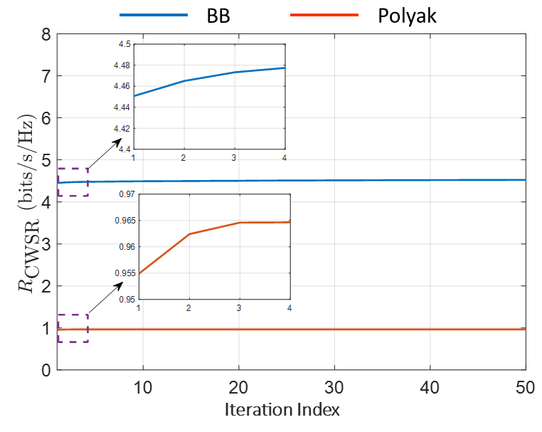
Figure 2 presents the convergence behavior of Algorithm 2 with two step-size rules: the BB algorithm and the Polyak’s rule, which shows that Algorithm 2 achieves a rapid convergence using both step-size rules because the co-phasing technique adopted for $\mathbf{v}_{\mathrm{d},j}$ uses the channel phase information, which aligns with initialization approach. It is also noted that the BB algorithm yields improved performance over that of Polyak’s rule.

Refer to caption
Figure 3: Proposed D-ISAC design approach compared with the conventional communications precoding and radar coding techniques given CSI errors.

6.2 D-ISAC overall system evaluation

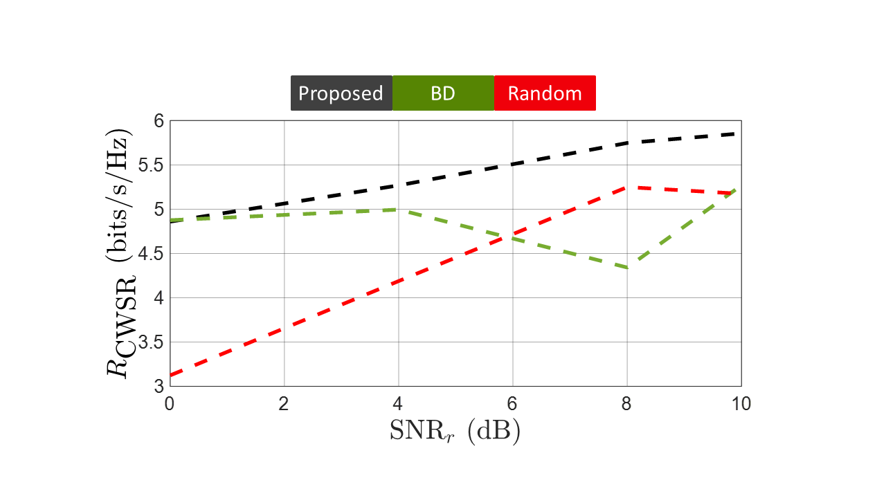
Figure3 demonstrates the overall D-ISAC system performance measured by (28) and the robustness of Algorithm 2 with channel estimation errors. We model the estimated channel vectors as $\widehat{\mathbf{h}}={\mathbf{h}}+\Delta$, where $\Delta\sim\mathcal{CN}\left({\mathbf{0},\eta^{2}_{\mathrm{CSI}}\mathbf{I}}\right)$ and $\mathbf{h}$ is referred to any of the small fading channel vectors introduced in Section 2.2 and $\eta^{2}_{\mathrm{CSI}}=0.1$ for this example. We also compare the proposed BCD-Alternating algorithm with conventional strategies, where we apply the block-diagonal (BD) beamforming technique to the DL beamformer $\mathbf{v}_{\mathrm{d},j}$ and the random radar coding scheme to the radar code matrix $\mathbf{A}$ (see the first companion paper [Part I] [22]), where the BD approach only applies to the DL beamforming; the proposed DL and UL beamforming is used with the random radar coding. The proposed D-ISAC design approach displays its overall robustness given the channel uncertainty and system-level advantage over other compared design approaches.

6.3 FD communications

Refer to caption
Figure 4: Proposed D-ISAC design approach compared with the conventional communications precoding and radar coding techniques given CSI errors.

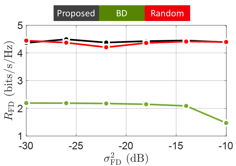
We then evaluate the impact of the FD communications on the FD C-RAN system, where Figure 4 depicts $R_{\mathrm{FD}}$ against the SI attenuation level $\sigma^{2}_{\mathrm{FD}}$ ranging from $-30$ to $-10$ dB, where $R_{\mathrm{FD}}$ represents the weighted achievable rate of the FD-CRAN system given by the second term on the right-hand-side of (28). Similar to the previous example, we consider the BD beamforming and radar random coding as benchmarks for our algorithm. As expected, the stronger the SI cancellation, the higher the FD C-RAN system achievable rate becomes. The FD C-RAN systems using the UL and DL beamformers based on our proposed algorithm outperform the one using the BD method for DL beamforming. Since the communications beamforming is applied to the radar random coding, we observe that the black and red curves share a similar trend in

6.4 Radar target data association

To evaluate the data association approach described in Section 5.2, we consider three sets of MIMO radar antenna array configurations. Further, we simulate the association probability for numerous targets in a 2D Cartesian plain.

We generate measurements following (52) for all Tx-Rx channels, where $P_{\mathrm{d}}=0.9$ and $P_{\mathrm{f}}=0.001$.

Refer to caption
Figure 5: Probability of correct association for different antenna geometries and number of targets.
Refer to caption
Figure 6: Ground truth and estimated location of three targets for L-shape Tx-Rx configuration.

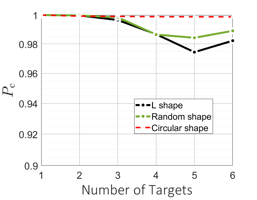
To quantify the performance of the proposed data association scheme, the probability of correct data association is defined as $P_{\mathrm{c}}=d_{\mathrm{c}}/D$, where $d_{\mathrm{c}}$ is the number of measurements associated to the correct targets, and $D$ is the number of total valid measurements. We compute $P_{\mathrm{c}}$ by varying the number of targets for three different popular array configurations (Circular, L-shape and Random) in Figure 5, where each curve is averaged over $2000$ MC realizations, in each realization $\left({x_{\mathrm{t},n_{\mathrm{t}}},y_{\mathrm{t},n_{\mathrm{t}}}}\right)$ is sampled randomly within a circle of radius $300$ $Km$ and $\sqrt{\dot{x}^{2}_{\mathrm{t},n_{\mathrm{t}}}+\dot{y}^{2}_{\mathrm{t},n_{\mathrm{t}}}}$ is uniformly generated within ${\left[{0,50}\right]}$ for all $n_{\mathrm{t}}$. In Figure 5, it can be noticed that among the three configurations, the circular configuration is the best in terms of the probability of correct association due to its $360^{\circ}$ coverage, and as expected, its performance degrades with the increase in the number of targets.

Refer to caption
Figure 7: Ground truth and estimated location of three targets in Circular Tx-Rx configuration.

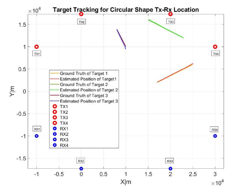
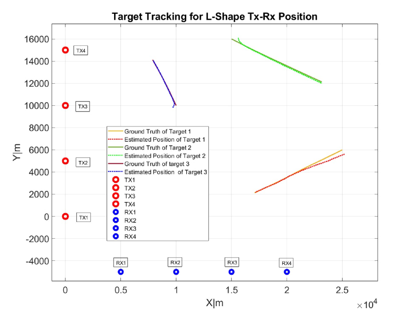
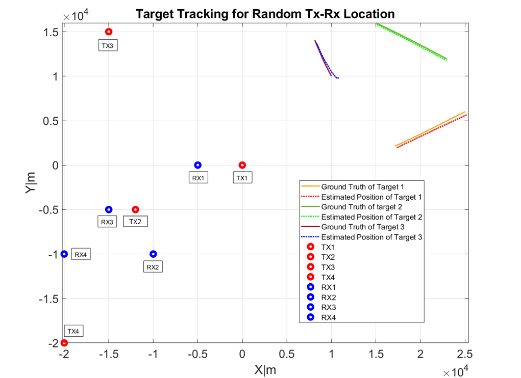
The performance efficacy of our distributed radar system for multi-target tracking was rigorously assessed via a series of numerical simulations. The experimental setup encompassed the tracking of three distinct targets, utilizing an array of four transmitters and four receivers. These components were strategically positioned in a variety of geometric configurations within a two-dimensional Cartesian coordinate system. Figures 6, 7 and  8 depict the simulated tracking scenario where Txs and Rxs are distributed in an L-shape, circular, and random configuration, respectively. The radar transmission frequency was set to 12 GHz for all the Txs with a 200 ms PRI. The $P_{\mathrm{fa}}$ was set to 0.001. The term $T$ denotes the interval of sampling, which we set to 200 ms. The probability of detection is assumed to be equal across every Tx-Rx pair.

For the L-shape, the Txs and Rxs are located as follows:

$$\mbox{Tx}_{m}=[0\quad(m-1)5]^{\top};\quad m=1,2,3,4\quad\mbox{and}\quad\mbox{Rx}_{n}=[5n\quad-5]^{\top};\quad n=1,2,3,4\,.$$

For the circular configuration, the transmitters and receivers are located as follows:

$$\mbox{Tx}_{1}=[-10\quad 10]^{\top};\quad\mbox{Tx}_{2}=[0\quad 17.32]^{\top};\quad\mbox{and}\quad\mbox{Tx}_{3}=[20\quad 17.32]^{\top};\quad\mbox{Tx}_{4}=[30\quad 10]^{\top}.$$
$$\mbox{Rx}_{1}=[-10\quad-10]^{\top};\quad\mbox{Rx}_{2}=[0\quad-17.32]^{\top};\quad\mbox{and}\quad\mbox{Rx}_{3}=[20\quad-17.32]^{\top};\quad\mbox{Rx}_{4}=[30\quad-10]^{\top}.$$

For the random configuration, the transmitters and receivers are located as follows:

$$\mbox{Tx}_{1}=[0\quad 0]^{\top};\quad\mbox{Tx}_{2}=[-10\quad-5]^{\top};\quad\mbox{and}\quad\mbox{Tx}_{3}=[-15\quad-5]^{\top};\quad\mbox{Tx}_{4}=[-20\quad-20]^{\top}.$$
Refer to caption
Figure 8: Ground truth and estimated location of three targets for Random Tx-Rx configuration.
$$\mbox{Rx}_{1}=[-5\quad 0]^{\top};\quad\mbox{Rx}_{2}=[-10\quad-10]^{\top};\quad\mbox{and}\quad\mbox{Rx}_{3}=[-15\quad-5]^{\top};\quad\mbox{Rx}_{4}=[-20\quad-10]^{\top}.$$

The targets follow a nearly constant velocity motion model, with initial states for target 1, target 2, and target 3 as, respectively,

$$[25\quad 6\,-0.4\,-0.2]^{\top};\quad[15\quad 16\quad 0.4\quad-0.2]^{\top};\quad[10\quad 10\quad-0.1\quad 0.2]^{\top}\,.$$

We consider the initial conditions for three targets and additional simulation parameters to be the same for all transmitter-receiver configurations.

6.5 Target tracking

Localization and tracking in MIMO radar depend on the target’s initial states and the geometry of the system [93]. Target tracking scenarios using the L-shape array configuration are shown in Figure 6, using Circular and Random array configurations can be found in Figure 7 and Figure 8, respectively. All these three figures suggest that in a distributed MIMO radar system, the circular array configuration is the most efficient in tracking the targets among the three array configurations. This observation agrees well with the results in Figure 5, where the probability of correct association has been investigated. This is because both performance metrics complement each other. Table 2 demonstrates the echo sequence for each target from the corresponding transmitter receiver for the circular transmitter-receiver configuration. Each receiver receives multiple echoes, which are unordered in nature. From the estimated target location using the JPDA algorithm, we estimate the order of echo at any receiver.

Table 2: Echo Sequence from three targets, before and after association.
$\mbox{Tx}_{1}$ $\mbox{Tx}_{2}$ $\mbox{Tx}_{3}$ $\mbox{Tx}_{4}$ After Association
$\mbox{Rx}_{1}$ target 3,2,1 target 3,2,1 target 2,3,1 target 1,3,2 3,2,1
$\mbox{Rx}_{2}$ target 3,2,1 target 3,2,1 target 2,3,1 target 1,3,2 3,2,1
$\mbox{Rx}_{3}$ target 3,2,1 target 3,2,1 target 2,1,3 target 1,2,3 1,3,2
$\mbox{Rx}_{4}$ target 3,1,2 target 3,2,1 target 1,2,3 target 1,2,3 1,3,2

Here, we notice that the joint association probability helps successfully associate each measurement with the corresponding targets.

7 Conclusion

This is a concluding paper of a three-part series. The first two companion papers Part I [22] and Part II [23] investigated, respectively, the signal processing and the synergistic design algorithm for a IBFD MU-MIMO communications system that shares spectrum with a distributed MIMO radar with a single target in its coverage area. In this paper, we handled the co-design challenge for a multiple target scenario. A method of low computational complexity, leveraging the Barzilai-Borwein gradient algorithm, was introduced to derive the design parameters efficiently. Furthermore, we employed a mixed-integer linear programming approach to facilitate distributed target localization. The feasibility and precision of multi-target sensing capabilities within the distributed IBFD ISAC framework were validated through comprehensive numerical experiments. Additionally, our study showcased the practical application of the IBFD MU-MIMO communication system and distributed radar ISAC system for localizing and tracking multiple targets, employing advanced techniques such as the JPDA and extended Kalman filter. Three different transmitter-receiver array (L-shape, circular, and random) configurations were considered. Among those, the circular configuration exhibited the best association and tracking performance because of its $360^{\circ}$ coverage of the surveillance area.

References

  • [1] A. T. Le, L. C. Tran, X. Huang, Y. J. Guo, Beam-based analog self-interference cancellation in full-duplex MIMO systems, IEEE Transactions on Wireless Communications 19 (4) (2020) 2460–2471.
  • [2] Z. Zhang, K. Long, A. V. Vasilakos, L. Hanzo, Full-duplex wireless communications: Challenges, solutions, and future research directions, Proceedings of the IEEE 104 (7) (2016) 1369–1409.
  • [3] L. Song, R. Wichman, Y. Li, Z. Han, Full-duplex communications and networks, Cambridge University Press, 2017.
  • [4] 3GPP Release 18 [online] (March 2022).
  • [5] K. V. Mishra, M. R. Bhavani Shankar, V. Koivunen, B. Ottersten, S. A. Vorobyov, Toward millimeter wave joint radar communications: A signal processing perspective, IEEE Signal Processing Magazine 36 (5) (2019) 100–114.
  • [6] S. H. Dokhanchi, B. S. Mysore, K. V. Mishra, B. Ottersten, A mmWave automotive joint radar-communications system, IEEE Transactions on Aerospace and Electronic Systems 55 (3) (2019) 1241–1260.
  • [7] G. Duggal, S. Vishwakarma, K. V. Mishra, S. S. Ram, Doppler-resilient 802.11ad-based ultra-short range automotive joint radar-communications system, IEEE Transactions on Aerospace and Electronic Systems 56 (5) (2020) 4035–4048.
  • [8] D. W. K. Ng, Y. Wu, R. Schober, Power efficient resource allocation for full-duplex radio distributed antenna networks, IEEE Transactions on Wireless Communications 15 (4) (2016) 2896–2911.
  • [9] K. Singh, S. Biswas, T. Ratnarajah, F. A. Khan, Transceiver design and power allocation for full-duplex MIMO communication systems with spectrum sharing radar, IEEE Transactions on Cognitive Communications and Networking 4 (3) (2018) 556–566.
  • [10] P. Aquilina, A. C. Cirik, T. Ratnarajah, Weighted sum rate maximization in full-duplex multi-user multi-cell MIMO networks, IEEE Transactions on Communications 65 (4) (2017) 1590–1608.
  • [11] S. A. Hassani, V. Lampu, K. Parashar, L. Anttila, A. Bourdoux, B. v. Liempd, M. Valkama, F. Horlin, S. Pollin, In-band full-duplex radar-communication system, IEEE Systems Journal 15 (1) (2021) 1086–1097.
  • [12] C. B. Barneto, S. D. Liyanaarachchi, M. Heino, T. Riihonen, M. Valkama, Full duplex radio/radar technology: The enabler for advanced joint communication and sensing, IEEE Wireless Communications 28 (1) (2021) 82–88.
  • [13] B. Li, A. Petropulu, Joint transmit designs for co-existence of MIMO wireless communications and sparse sensing radars in clutter, IEEE Transactions on Aerospace and Electronic Systems 53 (6) (2017) 2846–2864.
  • [14] S. Biswas, K. Singh, O. Taghizadeh, T. Ratnarajah, Coexistence of MIMO radar and FD MIMO cellular systems with QoS considerations, IEEE Transactions on Wireless Communications 17 (11) (2018) 7281–7294.
  • [15] J. Liu, K. V. Mishra, M. Saquib, Precoder design for joint in-band full-duplex MIMO communications and widely-distributed MIMO radar, in: International Conference on Communications, 2022, pp. 4679–4684.
  • [16] K. V. Mishra, Y. C. Eldar, E. Shoshan, M. Namer, M. Meltsin, A cognitive sub-Nyquist MIMO radar prototype, IEEE Transactions on Aerospace and Electronic Systems 56 (2) (2020) 937–955.
  • [17] J. Liu, M. Saquib, Joint transmit-receive beamspace design for colocated MIMO radar in the presence of deliberate jammers, in: 51st Asilomar Conf. Signals Syst. Comput., 2017, pp. 1152–1156.
  • [18] S. Sun, K. V. Mishra, A. P. Petropulu, Target estimation by exploiting low rank structure in widely separated MIMO radar, in: IEEE Radar Conference, 2019, pp. 1–6.
  • [19] J. Li, P. Stoica, MIMO radar with colocated antennas, IEEE Signal Processing Magazine 24 (5) (2007) 106–114.
  • [20] J. Liu, M. Saquib, Transmission design for a joint MIMO radar and MU-MIMO downlink communication system, in: IEEE Global Conference on Signal and Information Processing, 2018, pp. 196–200.
  • [21] S. Sun, Y. Hu, K. V. Mishra, A. P. Petropulu, Widely separated MIMO radar using matrix completion, IEEE Transactions on Radar Systems 2 (2024) 180–196.
  • [22] J. Liu, K. V. Mishra, M. Saquib, Co-designing statistical MIMO radar and in-band full-duplex multi-user MIMO communications – Part I: Signal processing, Signal ProcessingUnder review (2024).
  • [23] J. Liu, K. V. Mishra, M. Saquib, Co-designing statistical MIMO radar and in-band full-duplex multi-user MIMO communications – Part II: Joint precoder, radar code, and receive filters design, Signal ProcessingUnder review (2024).
  • [24] R. Mudumbai, J. Hespanha, U. Madhow, G. Barriac, Distributed transmit beamforming using feedback control, IEEE Transactions on Information Theory 56 (1) (2010) 411–426.
  • [25] R. D. Preuss, D. R. Brown, III, Two-way synchronization for coordinated multicell retrodirective downlink beamforming, IEEE Transactions on Signal Processing 59 (11) (2011) 5415–5427.
  • [26] J. Kong, F. T. Dagefu, B. M. Sadler, Coverage analysis of distributed beamforming with random phase offsets using Ginibre point process, IEEE Access 8 (2020) 134351–134362.
  • [27] J. Kong, F. T. Dagefu, B. M. Sadler, Distributed beamforming in the presence of adversaries, IEEE Transactions on Vehicular Technology 69 (9) (2020) 9682–9696.
  • [28] S. Hanna, D. Cabric, Distributed transmit beamforming: Design and demonstration from the lab to UAVs, IEEE Transactions on Wireless Communications 22 (2) (2023) 778–792.
  • [29] I. Ahmad, C. Sung, D. Kramarev, G. Lechner, H. Hajime Suzuki, I. Grivell, Outage probability and ergodic capacity of distributed transmit beamforming with imperfect CSI, IEEE Transactions on Vehicular Technology 71 (3) (2022) 3008–3019.
  • [30] A. Abrardo, G. Fodor, M. Moretti, Distributed digital and hybrid beamforming schemes with MMSE-SIC receivers for the MIMO interference channel, IEEE Transactions on Vehicular Technology 68 (7) (2019) 6790–6804.
  • [31] C. B. Barneto, T. Riihonen, S. D. Liyanaarachchi, M. Heino, N. González-Prelcic, M. Valkama, Beamformer design and optimization for full-duplex joint communication and sensing at mm-Waves, IEEE Transactions on Communications 70 (12) (2022) 8298–8312.
  • [32] J. A. Nanzer, R. L. Schmid, T. M. Comberiate, J. E. Hodkin, Open-loop coherent distributed arrays, IEEE Transactions on Microwave Theory and Techniques 65 (5) (2017) 1662–1672.
  • [33] M. I. Hasan, S. Nayemuzzaman, M. Saquib, Performance analysis of large aperture mMIMO UCCA arrays in a 5G user dense network, in: 2022 IEEE Future Networks World Forum (FNWF), 2022, pp. 526–531.
  • [34] R. U. Murshed, Z. B. Ashraf, A. H. Hridhon, K. Munasinghe, A. Jamalipour, M. F. Hossain, A CNN-LSTM-based fusion separation deep neural network for 6G ultra-massive MIMO hybrid beamforming, IEEE Access 11 (2023) 38614–38630.
  • [35] R. U. Murshed, M. S. Ullah, M. Saquib, M. Z. Win, Self-supervised contrastive learning for 6G UM-MIMO THz communications: Improving robustness under imperfect CSI, arXiv preprint arXiv:2401.11376 (2024).
  • [36] R. Chopra, C. R. Murthy, R. Annavajjala, Multistream distributed cophasing, IEEE Transactions on Signal Processing 65 (4) (2017) 1042–1057.
  • [37] J. Liu, K. V. Mishra, M. Saquib, Distributed beamforming for joint radar-communications, in: IEEE Sensor Array and Multichannel Signal Processing Workshop, 2022, pp. 151–155.
  • [38] Y. Yang, R. S. Blum, Phase synchronization for coherent MIMO radar: Algorithms and their analysis, IEEE Transactions on Signal Processing 59 (11) (2011) 5538–5557.
  • [39] H. Li, F. Wang, C. Zeng, M. A. Govoni, Signal detection in distributed MIMO radar with non-orthogonal waveforms and sync errors, IEEE Transactions on Signal Processing 69 (2021) 3671–3684.
  • [40] W. Khan, I. M. Qureshi, K. Sultan, Ambiguity function of phased-MIMO radar with colocated antennas and its properties, IEEE Geoscience and Remote Sensing Letters 11 (7) (2014) 1220–1224.
  • [41] H. Godrich, A. M. Haimovich, R. S. Blum, Target localization accuracy gain in MIMO radar-based systems, IEEE Transactions on Information Theory 56 (6) (2010) 2783–2803.
  • [42] R. Boyer, Performance bounds and angular resolution limit for the moving colocated MIMO radar, IEEE Transactions on Signal Processing 59 (4) (2011) 1539–1552.
  • [43] M. Dianat, M. R. Taban, J. Dianat, V. Sedighi, Target localization using least squares estimation for MIMO radars with widely separated antennas, IEEE Transactions on Aerospace and Electronic Systems 49 (4) (2013) 2730–2741.
  • [44] Q. He, R. S. Blum, H. Godrich, A. M. Haimovich, Target velocity estimation and antenna placement for MIMO radar with widely separated antennas, IEEE Journal of Selected Topics in Signal Processing 4 (1) (2010) 79–100.
  • [45] M. Akçakaya, A. Nehorai, MIMO radar detection and adaptive design under a phase synchronization mismatch, IEEE Transactions on Signal Processing 58 (10) (2010) 4994–5005.
  • [46] J. A. Nanzer, S. R. Mghabghab, S. M. Ellison, A. Schlegel, Distributed phased arrays: Challenges and recent advances, IEEE Transactions on Microwave Theory and Techniques 69 (11) (2021) 4893–4907.
  • [47] K. K. Chaythanya, R. Annavajjala, C. R. Murthy, Comparative analysis of pilot-assisted distributed cophasing approaches in wireless sensor networks, IEEE Transactions on Signal Processing 59 (8) (2011) 3722–3737.
  • [48] A. Manesh, C. R. Murthy, R. Annavajjala, Physical layer data fusion via distributed co-phasing with general signal constellations, IEEE Transactions on Signal Processing 63 (17) (2015) 4660–4672.
  • [49] Q. He, Z. Wang, J. Hu, R. S. Blum, Performance gains from cooperative MIMO radar and MIMO communication systems, IEEE Signal Processing Letters 26 (1) (2019) 194–198.
  • [50] C. D’Andrea, S. Buzzi, M. Lops, Communications and radar coexistence in the massive MIMO regime: Uplink analysis, IEEE Transactions on Wireless Communications 19 (1) (2020) 19–33.
  • [51] F. Liu, C. Masouros, A. Li, T. Ratnarajah, J. Zhou, MIMO radar and cellular coexistence: A power-efficient approach enabled by interference exploitation, IEEE Transactions on Signal Processing 66 (14) (2018) 3681–3695.
  • [52] Z. Xiao, Y. Zeng, Waveform design and performance analysis for full-duplex integrated sensing and communication, IEEE Journal on Selected Areas in Communications 40 (6) (2022) 1823–1837.
  • [53] S. Nayemuzzaman, K. V. Mishra, M. Saquib, Multi-target tracking for full-duplex distributed integrated sensing and communications, in: Asilomar Conference on Signals, Systems, and Computers, 2023, pp. 1–6.
  • [54] R. Fletcher, On the Barzilai-Borwein method, in: L. Qi, K. Teo, X. Yang (Eds.), Optimization and control with applications, Vol. 96 of Applied Optimization, Springer, 2005, pp. 235–256.
  • [55] A. Beck, L. Tetruashvili, On the convergence of block coordinate descent type methods, SIAM Journal on Optimization 23 (4) (2013) 2037–2060.
  • [56] S. A. R. Kazemi, R. Amiri, F. Behnia, Data association for multi-target elliptic localization in distributed MIMO radars, IEEE Communications Letters 25 (9) (2021) 2904–2907.
  • [57] M. Radmard, S. M. Karbasi, M. M. Nayebi, Data fusion in MIMO DVB-T-based passive coherent location, IEEE Transactions on Aerospace and Electronic Systems 49 (3) (2013) 1725–1737.
  • [58] Y. Kalkan, B. Baykal, Multiple target localization & data association for frequency-only widely separated MIMO radar, Digital Signal Processing 25 (2014) 51 – 61.
  • [59] U. Niesen, J. Unnikrishnan, Joint beamforming and association design for MIMO radar, IEEE Transactions on Signal Processing 67 (14) (2019) 3663–3675.
  • [60] S. S. Blackman, Multiple hypothesis tracking for multiple target tracking, IEEE Aerospace and Electronic Systems Magazine 19 (1) (2004) 5–18.
  • [61] R. P. Mahler, Multitarget Bayes filtering via first-order multitarget moments, IEEE Transactions on Aerospace and Electronic Systems 39 (4) (2003) 1152–1178.
  • [62] D. Musicki, R. Evans, S. Stankovic, Integrated probabilistic data association, IEEE Transactions on Automatic Control 39 (6) (1994) 1237–1241.
  • [63] M. Mohammadi, H. A. Suraweera, C. Tellambura, Uplink/downlink rate analysis and impact of power allocation for full-duplex Cloud-RANs, IEEE Transactions on Wireless Communications 17 (9) (2018) 5774–5788.
  • [64] A. M. Haimovich, R. S. Blum, L. J. Cimini, MIMO radar with widely separated antennas, IEEE Signal Processing Magazine 25 (1) (2008) 116–129.
  • [65] M. Radmard, M. M. Chitgarha, M. Nazari Majd, M. M. Nayebi, Ambiguity function of MIMO radar with widely separated antennas, in: International Radar Symposium, 2014, pp. 1–5.
  • [66] S.-R. Lee, S.-H. Moon, H.-B. Kong, I. Lee, Optimal beamforming schemes and its capacity behavior for downlink distributed antenna systems, IEEE Transactions on Wireless Communications 12 (6) (2013) 2578–2587.
  • [67] P. Kumari, J. Choi, N. González-Prelcic, R. W. Heath, IEEE 802.11ad-based radar: An approach to joint vehicular communication-radar system, IEEE Transactions on Vehicular Technology 67 (4) (2018) 2168–2181.
  • [68] P. Wang, H. Li, B. Himed, Moving target detection using distributed MIMO radar in clutter with nonhomogeneous power, IEEE Transactions on Signal Processing 59 (10) (2011) 4809–4820.
  • [69] S. Sun, W. U. Bajwa, A. P. Petropulu, MIMO-MC radar: A MIMO radar approach based on matrix completion, IEEE Transactions on Aerospace and Electronic Systems 51 (3) (2015) 1839–1852.
  • [70] J. A. Zhang, K. Wu, X. Huang, Y. J. Guo, D. Zhang, R. W. Heath, Integration of radar sensing into communications with asynchronous transceivers, IEEE Communications Magazine (2022) 1–7.
  • [71] B. Clerckx, C. Oestges, MIMO wireless networks: Channels, techniques and standards for multi-antenna, multi-user and multi-cell systems, Academic Press, Oxford, United Kingdom, 2013.
  • [72] M. Rihan, L. Huang, Optimum co-design of spectrum sharing between MIMO radar and MIMO communication systems: An interference alignment approach, IEEE Transactions on Vehicular Technology 67 (12) (2018) 11667–11680.
  • [73] Y. Cui, V. Koivunen, X. Jing, Interference alignment based spectrum sharing for MIMO radar and communication systems, in: IEEE International Workshop on Signal Processing Advances in Wireless Communications, 2018, pp. 1–5.
  • [74] M. Alaee-Kerahroodi, M. R. Bhavani Shankar, K. V. Mishra, B. Ottersten, Information theoretic approach for waveform design in coexisting MIMO radar and MIMO communications, in: IEEE Int. Conf. Acoust. Speech Signal Process., 2020, pp. 1–5.
  • [75] S. H. Dokhanchi, M. R. Bhavani Shankar, K. V. Mishra, B. Ottersten, Multi-constraint spectral co-design for colocated MIMO radar and MIMO communications, in: IEEE International Conference on Acoustics, Speech, and Signal Processing, 2020, pp. 4567–4571.
  • [76] Q. Shi, M. Razaviyayn, Z. Luo, C. He, An iteratively weighted MMSE approach to distributed sum-utility maximization for a MIMO interfering broadcast channel, IEEE Transactions on Signal Processing 59 (9) (2011) 4331–4340.
  • [77] M. R. Bell, Information theory and radar waveform design, IEEE Transactions on Information Theory 39 (5) (1993) 1578–1597.
  • [78] X. Song, P. Willett, S. Zhou, P. B. Luh, The MIMO radar and jammer games, IEEE Transactions on Signal Processing 60 (2) (2012) 687–699.
  • [79] M. M. Naghsh, M. Modarres-Hashemi, M. A. Kerahroodi, E. H. M. Alian, An information theoretic approach to robust constrained code design for MIMO radars, IEEE Transactions on Signal Processing 65 (14) (2017) 3647–3661.
  • [80] M. Mulla, A. H. Ulusoy, A. Rizaner, H. Amca, Barzilai-Borwein gradient algorithm based alternating minimization for single user millimeter wave systems, IEEE Communications Letters 9 (4) (2020) 508–512.
  • [81] Y. Park, S. Dhar, S. Boyd, M. Shah, Variable metric proximal gradient method with diagonal Barzilai-Borwein stepsize, in: IEEE International Conference on Acoustics, Speech, and Signal Processing, 2020, pp. 3597–3601.
  • [82] A. Robles-Kelly, A. Nazari, Incorporating the Barzilai-Borwein adaptive step size into sugradient methods for deep network training, in: Digital Image Computing: Techniques and Applications, 2019, pp. 1–6.
  • [83] O. Burdakov, Y. Dai, N. Huang, Stabilized Barzilai-Borwein method, Journal of Computational Mathematics 37 (6) (2019) 916.
  • [84] T. Zhang, G. Cui, L. Kong, X. Yang, Adaptive Bayesian detection using MIMO radar in spatially heterogeneous clutter, IEEE Signal Processing Letters 20 (6) (2013) 547–550.
  • [85] S. M. Kay, Fundamentals of statistical signal processing Volume II: Detection theory, Prentice-Hall, 1993.
  • [86] R. Deming, J. Schindler, L. Perlovsky, Multi-target/multi-sensor tracking using only range and Doppler measurements, IEEE Transactions on Aerospace and Electronic Systems 45 (2) (2009) 593–611.
  • [87] D. F. Crouse, P. Willett, Computation of target-measurement association probabilities using the matrix permanent, IEEE Transactions on Aerospace and Electronic Systems 53 (2) (2017) 698–702.
  • [88] Y. Bar-Shalom, X. R. Li, T. Kirubarajan, Estimation with applications to tracking and navigation: Theory algorithms and software, John Wiley & Sons, 2004.
  • [89] Y. F. Shi, T. L. Song, Sequential processing JIPDA for multitarget tracking in clutter using multistatic passive radar, in: International Conference on Information Fusion, 2016, pp. 711–718.
  • [90] S. Choi, C. R. Berger, D. Crouse, P. Willett, S. Zhou, Target tracking for multistatic radar with transmitter uncertainty, in: O. E. Drummond, R. D. Teichgraeber (Eds.), SPIE Signal and Data Processing of Small Targets, Vol. 7445, 2009, p. 74450M.
  • [91] S. Choi, D. F. Crouse, P. Willett, S. Zhou, Approaches to Cartesian data association passive radar tracking in a DAB/DVB network, IEEE Transactions on Aerospace and Electronic Systems 50 (1) (2014) 649–663.
  • [92] D. F. Crouse, Y. Bar-Shalom, P. Willett, L. Svensson, The JPDAF in practical systems: Computation and snake oil, in: O. E. Drummond (Ed.), SPIE Signal and Data Processing of Small Targets, Vol. 7698, 2010, p. 769813.
  • [93] M. Sadeghi, F. Behnia, R. Amiri, A. Farina, Target localization geometry gain in distributed MIMO radar, IEEE Transactions on Signal Processing 69 (2021) 1642–1652.