Quantum to Classical Neural Network Transfer Learning Applied to Drug Toxicity Prediction

Abstract

Toxicity is a roadblock that prevents an inordinate number of drugs from being used in potentially life-saving applications. Deep learning provides a promising solution to finding ideal drug candidates; however, the vastness of chemical space coupled with the underlying $\mathcal{O}(n^{3})$ matrix multiplication means these efforts quickly become computationally demanding. To remedy this, we present a hybrid quantum-classical neural network for predicting drug toxicity, utilizing a quantum circuit design that mimics classical neural behavior by explicitly calculating matrix products with complexity $\mathcal{O}(n^{2})$. Leveraging the Hadamard test for efficient inner product estimation rather than the conventionally used swap test, we reduce the number qubits by half and remove the need for quantum phase estimation. Directly computing matrix products quantum mechanically allows for learnable weights to be transferred from a quantum to a classical device for further training. We apply our framework to the Tox21 dataset and show that it achieves commensurate predictive accuracy to the model’s fully classical $\mathcal{O}(n^{3})$ analog. Additionally, we demonstrate the model continues to learn, without disruption, once transferred to a fully classical architecture. We believe combining the quantum advantage of reduced complexity and the classical advantage of noise-free calculation will pave the way to more scalable machine learning models.

Yale University] Department of Chemistry, Yale University, New Haven, 06511, CT, USA IR,NMR,UV

1 Introduction

The quest for novel pharmaceuticals is fraught with the challenge of ensuring drug safety. With 90% of drug candidates failing in clinical trials and 30% of these failures being attributed to toxicity¹, the cost to create a successful drug can exceed $2 billion USD², making the early detection of toxicological properties in drug candidates crucial.

Machine Learning (ML) has revolutionized the field of drug discovery^{3, 4, 5}, offering a powerful tool to handle and interpret the complex datasets that are characteristic of pharmaceutical research. By leveraging algorithms that can learn from and make predictions on data, ML has enabled significant advancements in identifying new drug candidates ^{6, 7, 8} and predicting drug toxicity ^{9, 10, 11, 12, 13, 14}. As ML continues to amaze, researchers are always searching for new computational tools to bolster the tractability and performance of their models.

Quantum computing, with its inherent capability to handle certain complex computations more efficiently than classical computing, emerges as a promising solution. Leveraging the principles of superposition and entanglement, quantum computing offers a new framework that potentially expands computational boundaries for ML. Recent work suggests that quantum ML (QML) models are more learnable and generalize better to unseen data than classical networks ^{15, 16, 17, 18}. In pursuit of these potential advantages, researchers have built numerous QML models to address a range of chemical and biological problems ^{19, 20, 21, 22, 23, 24, 25, 26, 27, 28}. More specifically, there have been several QML works that are trained to predict toxicity ^{29, 10, 30}. Despite the success of these QML models, the limitations that plague noisy intermediate-scale quantum (NISQ) devices such as decoherence and gate errors are still a sobering reality.

While noise is not a concern for classical computing, it is not without its bottleneck either. Every year, as developers create deep learning models more powerful than the last, we are seeing a swift increase in the number of parameters ³¹. This escalation in parameter count introduces a consequential challenge: the need for significantly more computing power and the development of more efficient algorithms. Matrix multiplication lies at the heart of neural networks. The standard method of matrix multiplication has complexity $\mathcal{O}(n^{3})$, and while sub-cubic algorithms do exist such as the Strassen algorithm³² $\mathcal{O}(n^{2.8074})$ and the recording-setting algorithm by Williams et al.³³ $\mathcal{O}(n^{2.3716})$, these methods suffer from numerical instability³⁴, high memory usage, or have a complexity prefactor that makes them galactic algorithms, rending them impractical for tractable computation.

In response to these computational challenges, this study introduces a hybrid quantum-classical neural network model designed to leverage the strengths of both quantum and classical computing paradigms and apply the framework to drug toxicity prediction. Utilizing the Hadamard test, our model employs quantum circuits that replicate the forward functionality of classical neural networks, allowing the model to efficiently calculate discrete inner products. Assuming efficient state preparation, the swap test has been shown to be the most computationally favorable algorithm ³⁵ for matrix multiplication with complexity $\mathcal{O}(n^{2})$, and has been suggested for use in a quantum neuron ^{36, 37, 38, 39} . Our use of the Hadamard test achieves the same complexity, one quantum circuit for each dot product, while using half the working qubits and without the need for quantum phase estimation. This QML approach allows for “classical weights” to be easily derived from the quantum model, which can then be transferred to a classical machine to be fine-tuned without the presence of noise and errors which is characteristic of current NISQ devices. All previous works of quantum transfer learning are either classical-to-quantum ^{40, 41, 42}, or simply use the initial quantum component as a feature extractor that is non-learnable after transferring ⁴⁰. To our knowledge, this framework of fine-tuning weights classically that were initially embedded in a quantum circuit is a novel contribution to this growing field of quantum transfer learning.

In an effort to realize these potential quantum advantages, we investigate our model’s performance on drug toxicity prediction using the Tox21 dataset ^{43, 44} with a convolutional neural network (CNN). We present the effectiveness of our quantum CNN (QCNN), which replaces the filter with a quantum circuit to compute the dot product. Additionally, we illustrate that a classical convolution filter can seamlessly continue the training process initially started by its quantum counterpart. Furthermore, we demonstrate that both the hybrid quantum-classical model and the fully classical equivalents exhibit comparable performance levels for drug toxicity prediction.

2 Quadratic Matrix Multiplication

2.1 The Swap Test

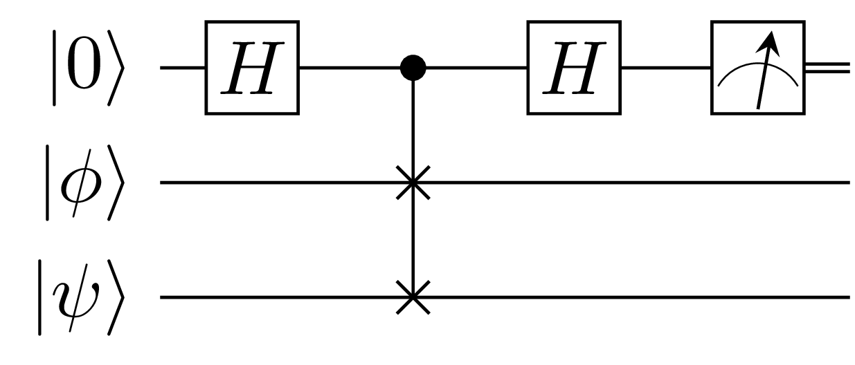
Figure 1: The Swap Test

The swap test⁴⁵, shown in Figure 1, has been suggested for use in a quantum neuron and as a convolutional filter ^{36, 37, 38, 39}. This idea is manifested by encoding the input data into one working register of qubits and by applying learnable quantum gates to another register. When the controlled swap between the two states of these registers is executed, the expectation value of the ancilla qubit will produce the squared modulus of the inner-product between the two states $\left|\braket{\phi}{\psi}\right|^{2}$ with error $\epsilon$, in $\mathcal{O}(\frac{1}{\epsilon^{2}})$ repetitions. In this sense, the amplitudes of the parameterized qubit register can be thought of analogously as the “weights”. These “weights” are being multiplied together with the input data and summed when the swap test is conducted and the ancilla is measured. However since the swap test only reveals the fidelity between two quantum states, it is directionless. The lack of the dot-product’s sign is problematic for flexible machine learning, and places additional difficulty on the learning procedure. A remedy to this is quantum phase estimation (QPE), but the extra ancilla qubits required in QPE place an additional overhead on the required resources to run this algorithm.

2.2 The Hadamard Test

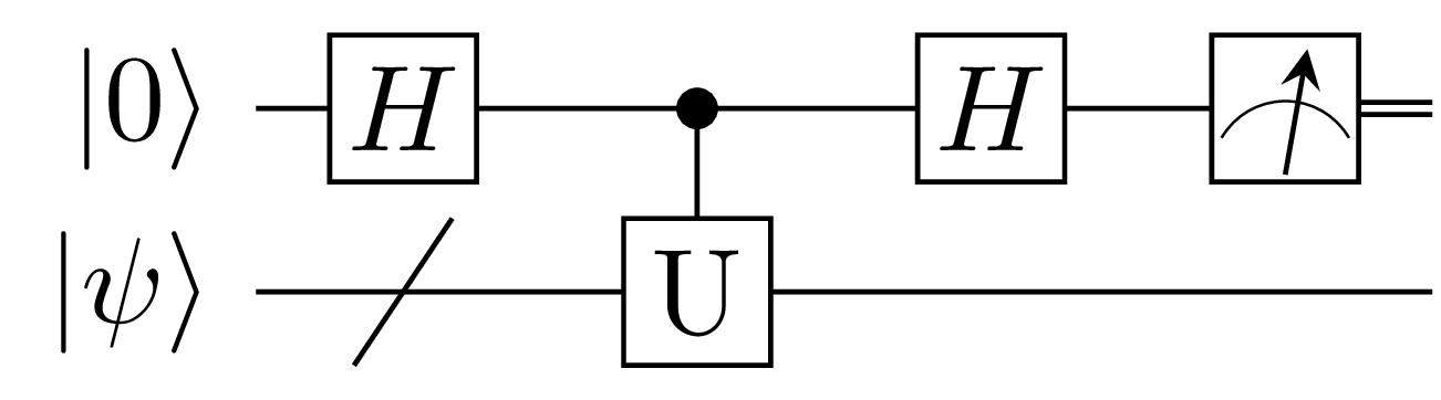
Figure 2: The Hadamard Test

The Hadamard test, shown in Figure 2, is another cornerstone quantum algorithm that allows one to determine $\text{Re}\braket{\psi}{U}{\psi}$ with error $\epsilon$, in $\mathcal{O}(\frac{1}{\epsilon^{2}})$ repetitions. However, by choosing the correct $U$, we can use this algorithm to produce the inner product between two vectors of choice, $\text{Re}\braket{\psi}{\phi}$. Since this gives a direction with the inner product unlike the swap test, we may dispense with the need for QPE as well as the need for separate quantum registers for the input data and parametric “weights”. Equations 1-4 show how $U$ can be chosen, for input data, $\ket{\phi}$ and “weights”, $\ket{\psi}$.

$$U_{\psi}\ket{0}^{\otimes n}=\ket{\psi}$$ (1)

$$U_{\phi}\ket{0}^{\otimes n}=\ket{\phi}$$ (2)

$$U=U_{\phi}U^{\dagger}_{\psi}$$ (3)

$$\operatorname{Re}\bra{\psi}U\ket{\psi}=\operatorname{Re}\bra{\psi}U_{\phi}U^{\dagger}_{\psi}\ket{\psi}=\operatorname{Re}\bra{\psi}U_{\phi}U^{\dagger}_{\psi}U_{\psi}\ket{0}^{\otimes n}=\operatorname{Re}\braket{\psi}{\phi}$$ (4)

Equation 4 shows that if $U$ is chosen to be the product of the unitary matrix that prepares the quantum state whose amplitudes act as the “weights” and the adjoint of the unitary that prepares the input data, the real part of the desired inner-product is obtained when performing the Hadamard test. This circuit is visualized in Figure 3.

We note that the full complex-valued inner product $\braket{\psi}{\phi}$ may easily be obtained. The Hadamard test may be slightly modified to include an $S^{\dagger}$ gate after the first Hadamard gate on the ancilla qubit to produce $\operatorname{Im}\braket{\psi}{\phi}$. Summing the expectation values of these two different Hadamard tests yields the complex-valued inner product $\operatorname{Re}\braket{\psi}{\phi}+i\operatorname{Im}\braket{\psi}{\phi}=\braket{\psi}{\phi}$.

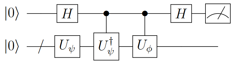
Figure 3: Quadratic Matrix Multiplication with the Hadamard Test

As with the swap test, only one quantum circuit needs to be run for each resulting entry (or two circuits for complex-valued input data) when finding the product of two matrices, and thus scales $\mathcal{O}(n^{2})$. While this method uses significantly fewer qubits than the swap test, it may come at the expense of deeper circuitry due to the controlled unitary gate $U^{\dagger}_{\psi}$ required to uncompute the input state. To this point, we note that both the swap test and the proposed Hadamard test method for multiplying arbitrary matrices with $\mathcal{O}(n^{2})$ complexity rely on the assumption of efficiently prepared quantum states ³⁵. As state preparation techniques become more refined, qubit control improves, and quantum devices become more coherent, the fulfillment of this assumption will also satisfy the concerns of deeper circuitry possessed by this Hadamard test method. Concurrently, the computational overhead of more than double the number of qubits and the requirement for QPE associated with the swap test will not be alleviated, as these are fundamental to the algorithm and are not dependent on quantum hardware.

3 Architecture and Dataset

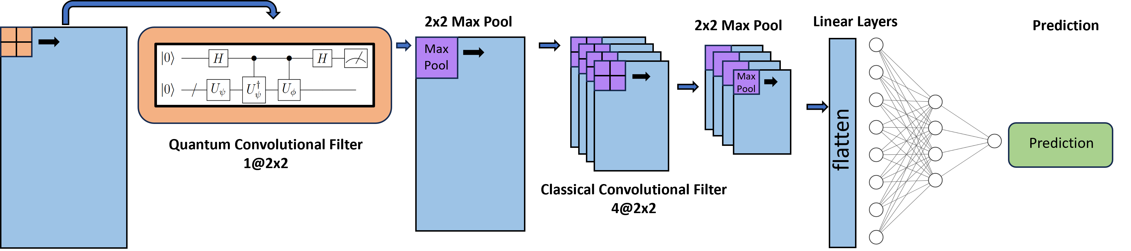
Figure 4: Quantum-Classical Neural Network Architecture

3.1 Hybrid Architecture

CNNs have been found to be successful for use in toxicity prediction tasks in the literature^{46, 47, 48}, and are very popular QML analogs of classical architectures ^{49, 50, 51, 52, 53}. The popularity of QCNNs partly stem from only needing to operate on small sections of input data at a time, rendering them feasible for NISQ devices. We employ a quantum-classical architecture where the first convolutional layer is replaced by a quantum circuit and is subsequently followed by classical pooling, a classical convolutional layer, and fully connected layers as depicted in Figure 4.

3.2 Tox21 Dataset

The Tox21 10k dataset ^{43, 44} is frequently used as a benchmark for evaluating ML models on their binary predictive ability for toxicity. This dataset comprises approximately 10,000 molecules represented as SMILES strings, each tagged with binary labels according to their response to 12 distinct assays. The Tox21 dataset suffers from significant imbalance, and although techniques such as SMOTE ⁵⁴ can enhance performance, the primary objective of this study is to showcase the synergy between quantum and classical ML frameworks, rather than attaining the highest level of predictive accuracy. We specifically choose to create a sparse, binary feature map from each SMILES string in order to reduce overhead on the quantum component of the model. The computational benefit of binary features in a CNN is visually depicted in Figure 5. For each filter comprised of $w$ weights, there can exist a maximum of $2^{w}$ unique convolutions for binary data. Thus, for a single 2 $\times$ 2 filter there are only 16 unique dot-products that are required to fully stride across input data of any size. Additionally, the sparsity condition allows for the use of state-preparation techniques that do not scale exponentially ^{55, 56}, which is a necessity along the road to achieving implementable quadratic complexity for matrix multiplication.

Feature type	Element	Bit(s)
Symbol in SMILES	( )	2
	[ ]	2
		1
	:	1
	=	1
	#	1
	\	1
	/	1
	@	1
	+	1
	-	1
	.	1
Number in SMILES	Atom Charge (2–7)	6
	Ring being (yes/no)	1
	Ring end (yes/no)	1
Atom type	C, H, O, N, others	5
Others	Surrounding Hydrogen Number (0–3)	4
	Atom Formal Charge (-1, 0, 1)	3
	Valence (1–5, other)	6
	Ring Atom (yes/no)	1
	Degree (1–4, other)	5
	Aromaticity (yes/no)	1
	Chirality (R/S/others)	3
	Hybridization (sp, sp2, sp3, sp3d, sp3d2, unspecified, other)	7
Total	-	57

Table 1: Feature Encoding Scheme for each SMILES Character

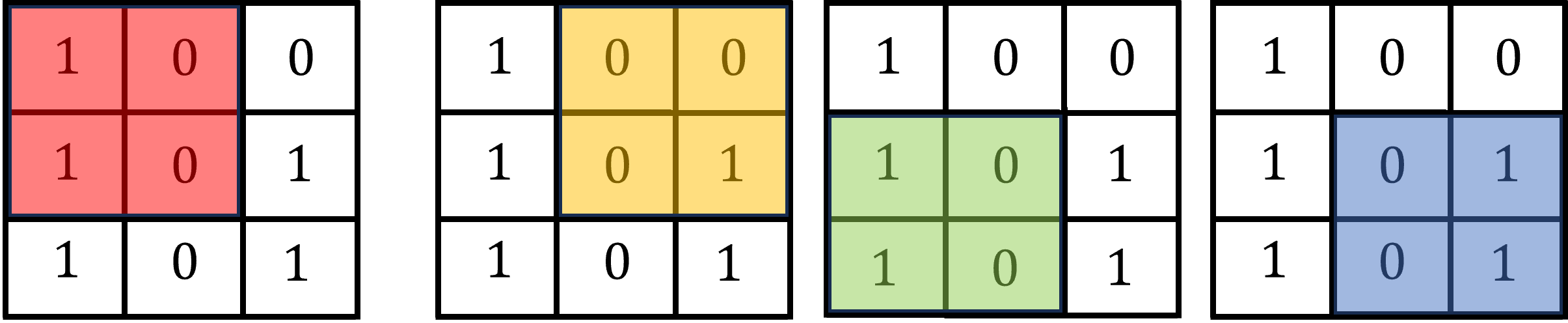
Figure 5: Binary data in a CNN. The red and green sections of this example input data will result in an identical output. For our input data of size 400 $\times$ 57 and a single 2 $\times$ 2 filter, we only need to execute 15 circuits (the all-zero vector need not be computed), rather than 22,344 for each molecule.

In this study, we utilize the Binary-Encoded-SMILES (BES) approach ⁴⁶, whereby each character within the SMILES string is depicted as a bit vector. 27 bits are used to encode the SMILES symbols and alphabet, and 30 bits are used to encode atomic properties. The vector of each character is joined with all other character vectors forming a grid, and is padded to the longest string in the dataset. The descriptors used to create this length 57 vector for each SMILES character are detailed in Table 1.

3.3 Quantum Transfer Learning

After training the quantum neural network (QNN), the real part of the first column of the unitary matrix $U_{\phi^{\prime}}$ that prepares the learned state $\ket{\phi^{\prime}}$ are the classical weights that may be used to further train the model on a classical device. This is the case since $U_{\phi^{\prime}}$ always operates on $\ket{0}^{\otimes n}$, which yields only the first column of $U_{\phi^{\prime}}$. Since the input data used in each quantum circuit must be L2 normalized to represent a valid quantum state, the corresponding classical component of the model must also work with normalized data to ensure a seamless transfer process. With regard to a CNN, this entails normalizing the data covered by a filter before taking the convolution with the weights, and is shown in Equation 5. $\left|\mathbb{x}\right|_{2}$ is the normalized input data, $x_{k}$ is the $k$-th element of the $n$-dimensional input data vector, and $\mathbb{w}$ is the weight vector from the flattened convolutional filter.

$$\text{output}=\left|\mathbb{x}\right|_{2}\cdot\mathbb{w}=\left(\sqrt{\sum_{k=1}^{n}\left|x_{k}\right|^{2}}\right)\cdot\mathbb{w}$$ (5)

The workflow of training and transferring our Hadamard test-based model from a hybrid QNN to a fully classical network is demonstrated in Figure 6. The details of the quantum component of the hybrid architecture are shown in Figure 7.

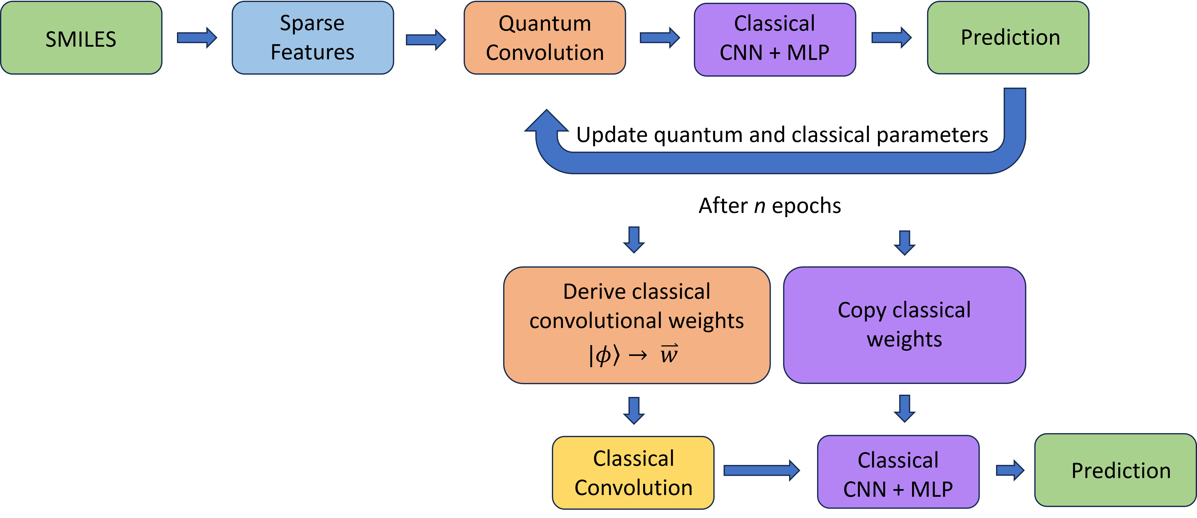
Figure 6: Quantum to classical neural network transfer pipeline. The yellow classical convolutional block L2-normalizes the input data covered by each filter to ensure a mathematically exact learning transition between quantum and classical computations.

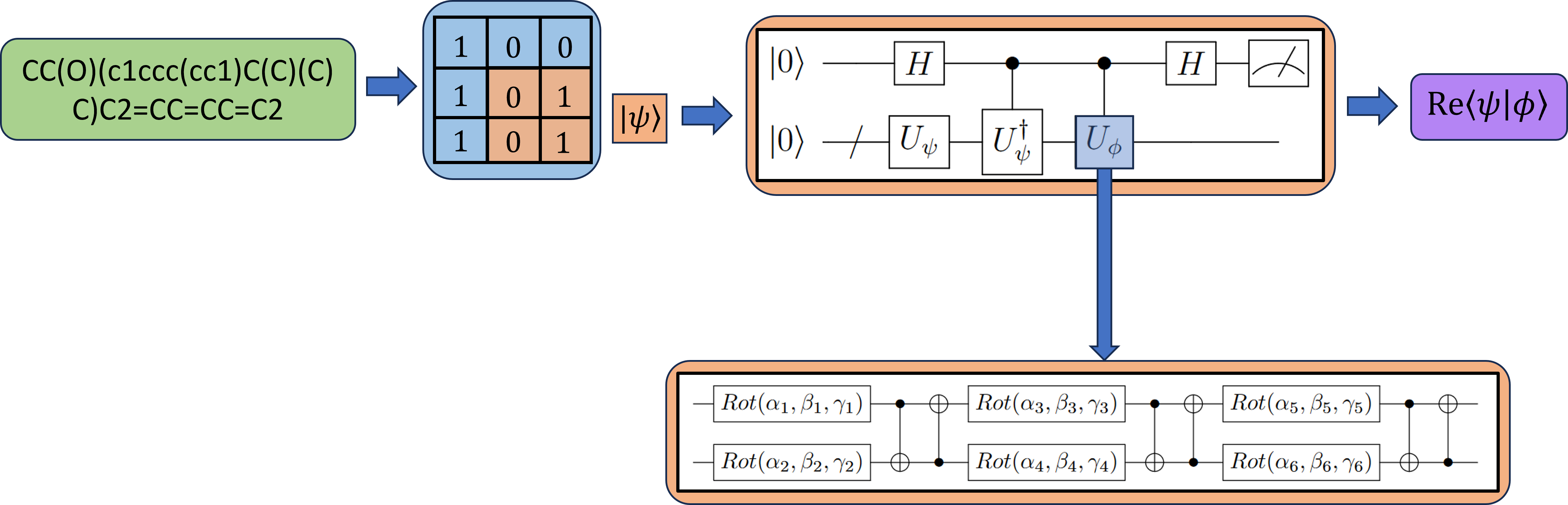
Figure 7: The variational quantum circuit used in the Hadamard test to calculate the real part of the inner product between an input data vector, $\ket{\psi}$ and a learnable weight vector $\ket{\phi}$. The unitary matrix of the Rot gate is shown in Equation 8.

4 Methods

4.1 Hardware

All scripting was done in Python 3.9.18. The quantum simulation package Pennylane ⁵⁷ version 0.35.0 was used, as well as PyTorch ⁵⁸ version 2.1.0 with CUDA Toolkit ⁵⁹ 11.8 . An Intel i7-13700KF CPU, 12GB Nvidia GeForce RTX 3080Ti GPU, and 64GB of 3600MHz CL18 RAM were used for all computations.

4.2 Dataset

The Tox21 dataset was downloaded from the National Institute of Health ⁴⁴. RDKit version 2023.09.1 was used to load the SMILES string and calculate the atomic features shown in Table 1. SMILES strings with invalid valence shells and deuterium isotopes were discarded. 80% of each assay dataset was used for training and 20% for the test set. To ensure all binary encoded SMILES were the same dimension, they were padded with zeros for a final shape of 400 $\times$ 57.

4.3 Machine Learning

Binary cross entropy was used for the loss function and weights were updated with the Adam optimizer ⁶⁰. A learning rate of 0.001 was used. Quantum weights were initialized from a uniform distribution between $0$ and $2\pi$. To ensure fair comparisons between the quantum and classical models, all other classical parameters were randomly initialized and copied to be identical between the models. The exponential decay rate for the first and second moment estimations were set to 0.9 and 0.999, respectively for all training. Epsilon was set to 1.0 $\times$ $10^{-8}$. The bias component of the quantum convolutional layer was trained classically. The output of each hidden layer in the model architecture was activated with ReLU. Given the imbalanced nature of the binary dataset, we find it appropriate to measure performance with the area under the curve of the receiver operating characteristic (ROC-AUC) ⁶¹. This metric calculates the area under the curve of the plot of the true positive rate (Equation 6) versus the false positive rate (Equation 7). An ROC-AUC score of $1.0$ indicates the model predicts all samples correctly, while a score of $0.5$ indicates the model is no better than random chance.

$$TPR=\frac{\text{True Positive}}{\text{True Positive}+\text{False Negative}}$$ (6)

$$FPR=\frac{\text{False Positive}}{\text{False Positive}+\text{True Negative}}$$ (7)

4.4 Quantum Computing

Quantum states were prepared with the algorithm presented by Mottonen et al. ⁶² available in Pennylane, however in practice with this feature map, the algorithms by Veras et al. ⁵⁵ and Gleinig et al. ⁵⁶ would be better suited for use with NISQ devices. The variational component of the quantum circuit used three layers from Pennylane’s StronglyEntanglingLayers, inspired by Schuld et al. ⁶³. The unitary matrices comprising the general rotation gates are show in Equations 8 and 9.

$$Rot\left(\alpha,\beta,\gamma\right)=RZ\left(\gamma\right)RY\left(\beta\right)RZ\left(\alpha\right)$$ (8)

$$RZ\left(\alpha\right)=\begin{bmatrix}e^{-i\frac{\alpha}{2}}&0\\ 0&e^{i\frac{\alpha}{2}}\\ \end{bmatrix},RY\left(\beta\right)=\begin{bmatrix}\cos{\left(\frac{\beta}{2}\right)}&-\sin{\left(\frac{\beta}{2}\right)}\\ \sin{\left(\frac{\beta}{2}\right)}&\cos{\left(\frac{\beta}{2}\right)}\\ \end{bmatrix}$$ (9)

The expectation value of the ancilla qubit in the computational basis was used as the input to the subsequent convolutional layer.

5 Results and Discussion

We compare our results to a fully classical model with identical architecture, except where the quantum convolutional filter is replaced by a classical filter of the same dimensions. It is shown in Table 2 that the QNN and CNN perform similarly for each assay. On the overall dataset, the quantum and classical models achieved an ROC-AUC of 0.692 and 0.689, respectively. These results demonstrate that the same accuracy as the classical $\mathcal{O}(n^{3})$ CNN can be achieved by the more efficient $\mathcal{O}(n^{2})$ quantum component of the model.

Table 2: Tox21 Test ROC-AUC

Assay	QNN	CNN	QNN transferred to CNN
nr-ahr	0.619	0.632	0.619
nr-ar	0.725	0.764	0.727
nr-ar-lbd	0.800	0.847	0.800
nr-aromatase	0.724	0.722	0.726
nr-er	0.677	0.674	0.676
nr-er-lbd	0.641	0.623	0.640
nr-ppar-gamma	0.636	0.586	0.626
sr-are	0.701	0.705	0.701
sr-atad5	0.682	0.644	0.679
sr-hse	0.677	0.668	0.675
sr-mmp	0.722	0.698	0.721
sr-p53	0.692	0.689	0.691
Average	0.692	0.689	0.691

Additionally, we demonstrate that the fully classical model is able to resume the training process started by the quantum model. As shown in Figures 8(a) and 8(b), the training continues seamlessly after 5 epochs, where weights for the classical convolutional filter were derived from Equation 2. The training curves for all assays are made available in the Supplemental Information.

(a)

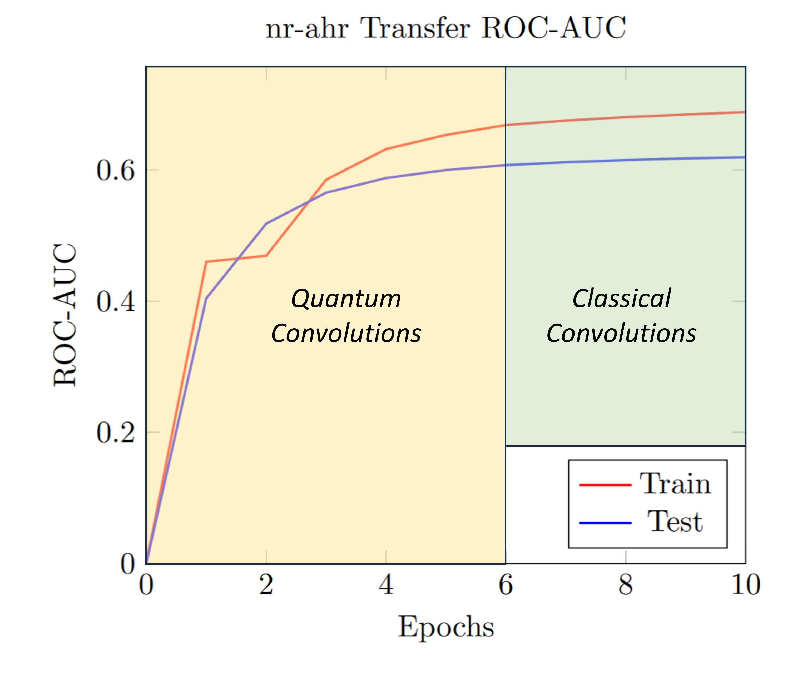
(b)

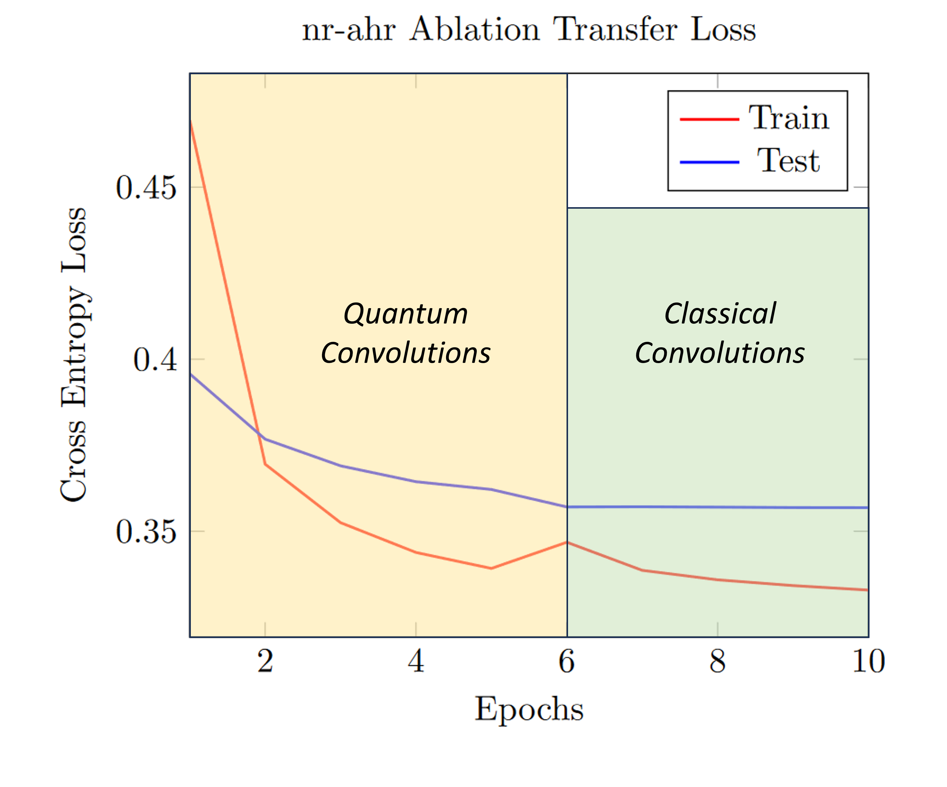
(c)

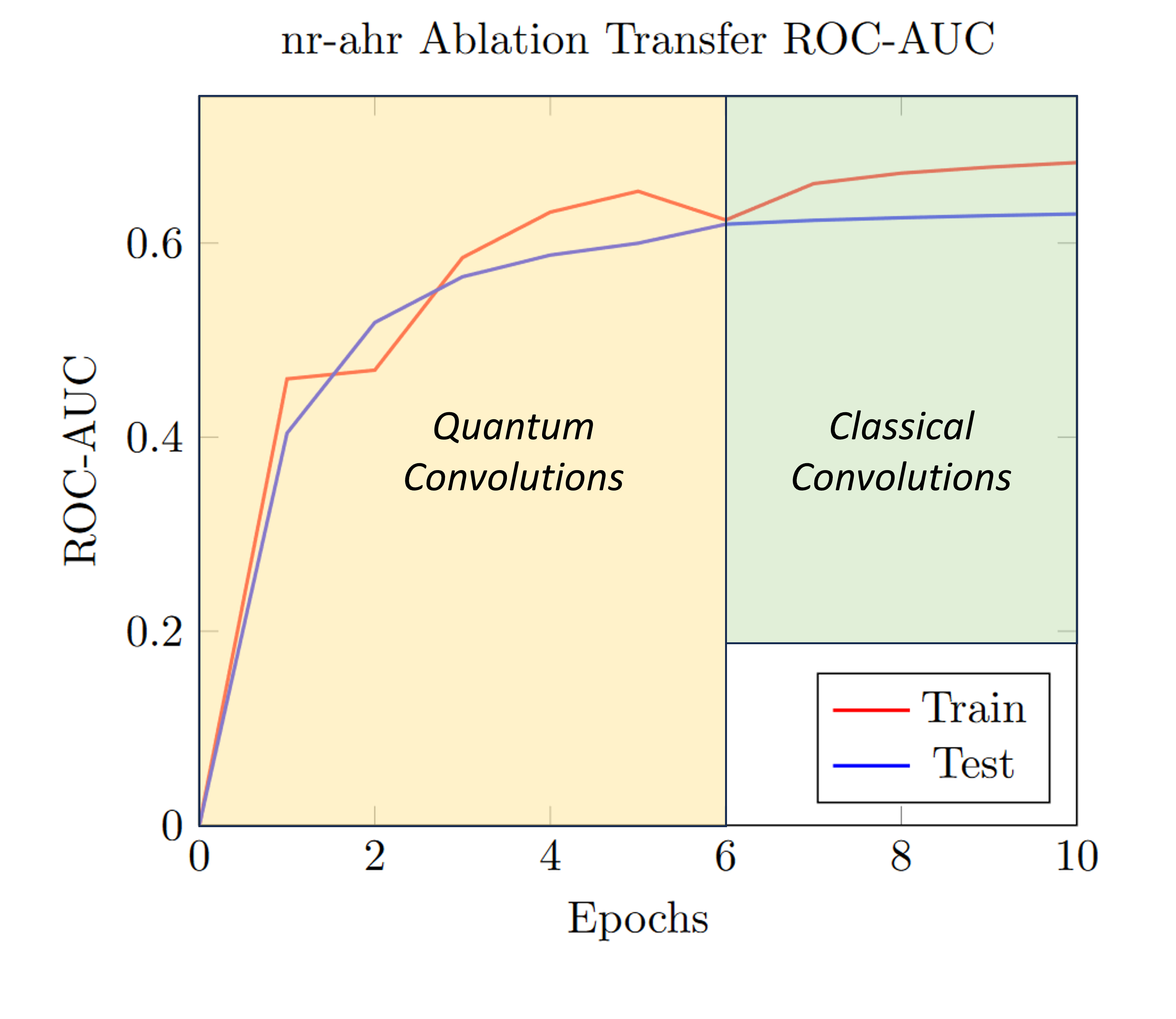
(d)

Figure 8: Model performance before and after weight transfer and ablation study results. (a) Transfer learning loss, (b) Transfer learning ROC-AUC, (c) Ablation study loss, (d) Ablation study ROC-AUC. The yellow shading (Epochs 1-5) indicates where the model was trained with quantum convolutions. The green shading (Epochs 6-10) indicates where the model was trained with classical convolutions. The ablation study (c and d) shows the model’s performance where the weights from the quantum layer were initialized to random values instead of deriving them from $U_{\phi}$.

The first convolutional layer transferred from quantum training to classical training contains only a small portion of the model’s total parameters. Despite this, the first layer of feature extraction plays a crucial role in the model’s overall performance, and improperly computing the weights during the transfer procedure will have a demonstrable impact. To validate our framework of properly transferring these weights, we show the resulting model’s performance after randomly initializing the weights from the first convolutional layer, while copying the remaining learned weights. Epoch 6, the first epoch after transferring to a fully classical architecture, shows a spike in cross entropy loss and a decrease in ROC-AUC in Figures 8(c) and 8(d). Despite being so few parameters, this ablation study is indicative that our framework correctly transfers these weights to be fine-tuned classically.

6 Conclusions

In summary, we present the first quantum-to-classical transfer learning framework where weights initially learned from a quantum circuit can be fine-tuned classically. We find quantum advantage by reducing the complexity of calculating matrix products from $\mathcal{O}(n^{3})$ to $\mathcal{O}(n^{2})$ using a modified version of the Hadamard test, which uses half the qubits of the previously proposed swap test for a quantum neuron and without the need for quantum phase estimation. We apply these methods to toxicity prediction using the Tox21 dataset, and show that our frameworks perform equivalently to a fully classical model with approximately the same number of parameters. As quantum devices improve, we hope this framework will provide an implementable polynomial speedup for machine learning networks, and consequently more efficiently navigate the chemical space to find life-saving pharmaceuticals.

7 Data and Software Availability

The data and code to reproduce the results presented here are available as open-source at https://github.com/anthonysmaldone/Quantum-to-Classical-Transfer-Learning.

8 Author Contributions

AMS designed the idea, AMS developed the software, AMS conducted the research, AMS and VSB analyzed the data, AMS wrote the article.

9 Acknowledgements

We acknowledge financial support from the National Institute of Health Biophysical Training Grant (1T32GM149438-01) [AS], as well as the financial support provided by the CCI Phase I: National Science Foundation Center for Quantum Dynamics on Modular Quantum Devices (CQD-MQD) under Award Number 2124511 [VSB]. Furthermore, we acknowledge seed funding from Yale University through the National Science Foundation Engines Development Award: Advancing Quantum Technologies (CT) under Award Number 2302908 and high-performance computer time from the National Energy Research Scientific Computing Center and from the Yale University Faculty of Arts and Sciences High Performance Computing Center.

10 Supplemental Information

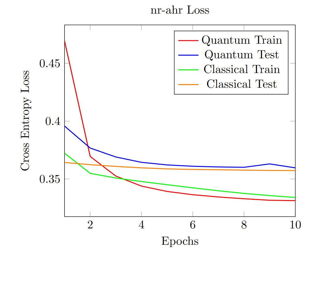
(a)

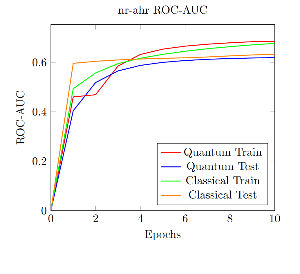
(b)

Figure S1: Training curves for the nr-ahr assay

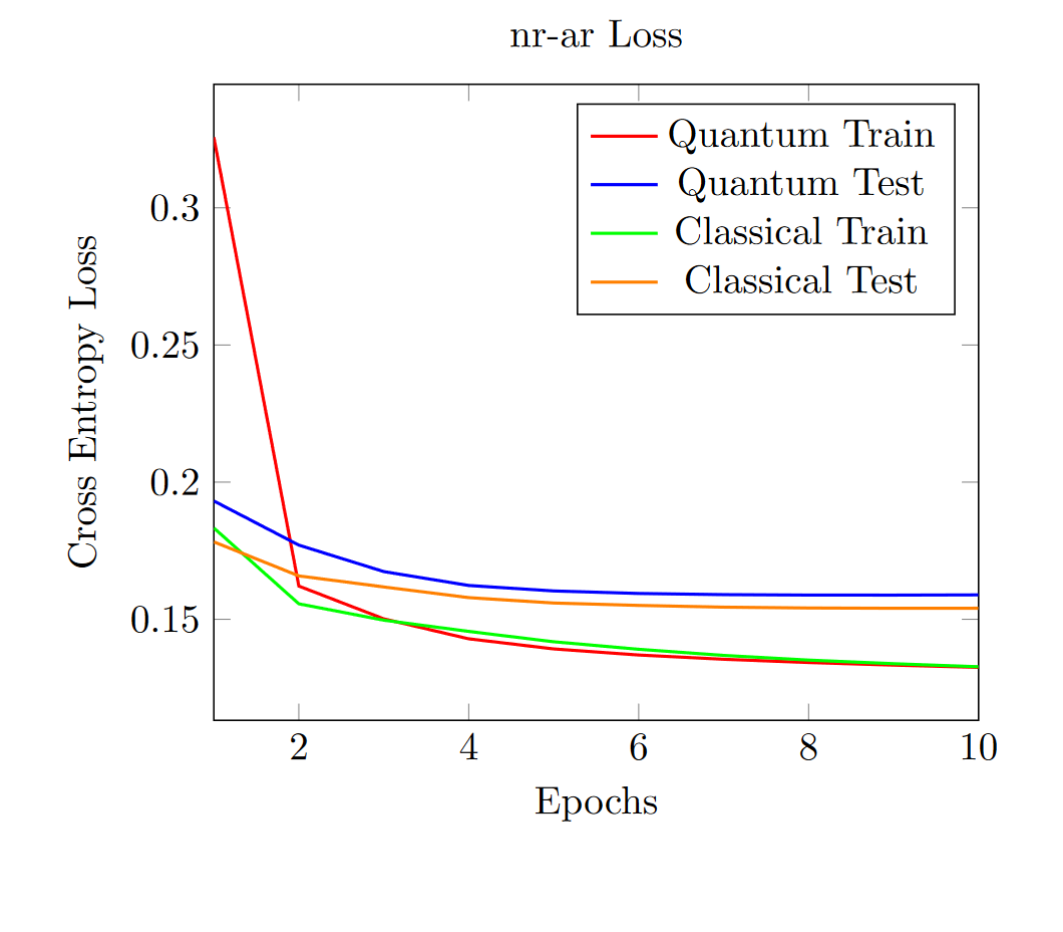
(a)

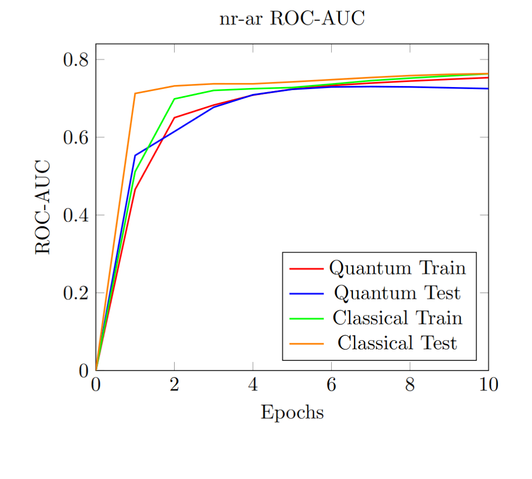
(b)

(c)

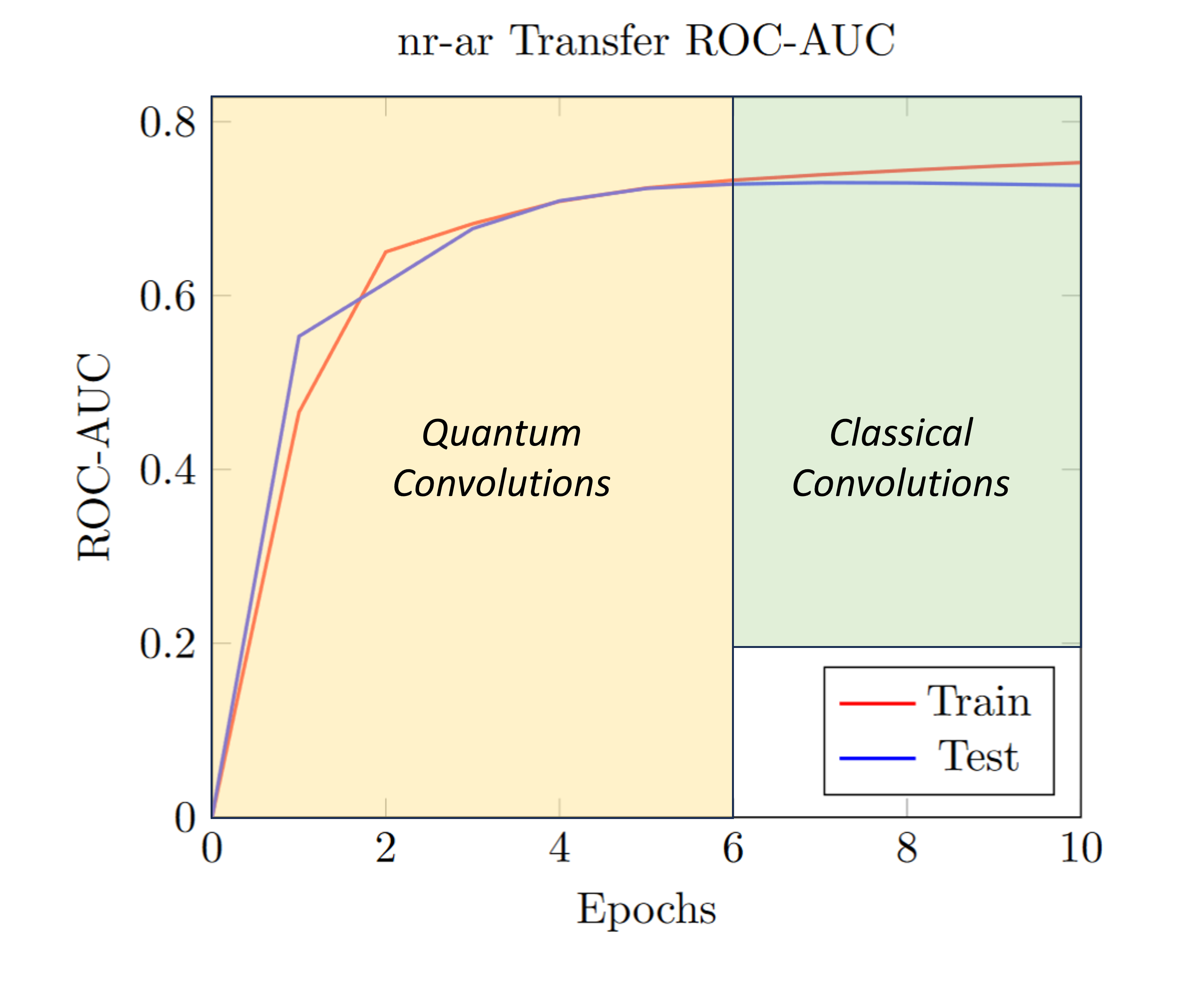
(d)

Figure S2: Training curves for the nr-ar assay

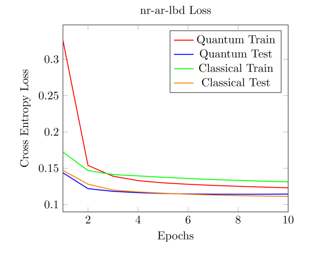
(a)

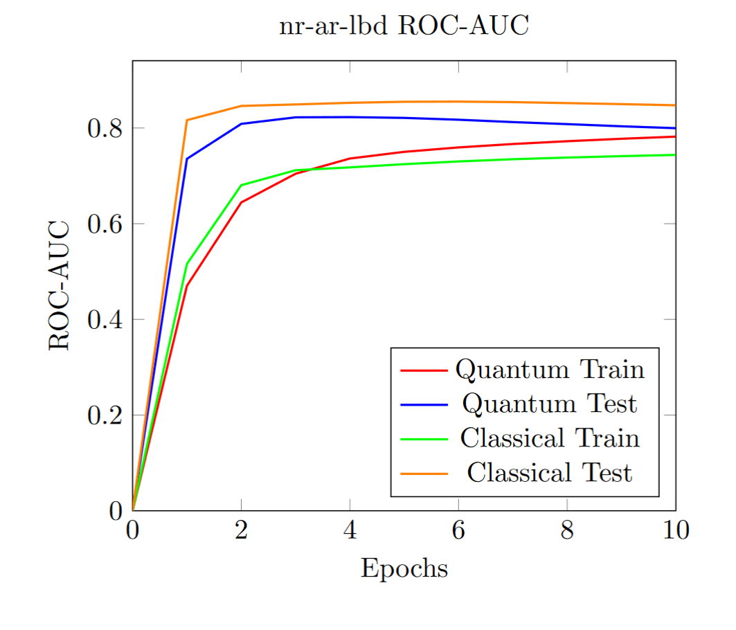
(b)

(c)

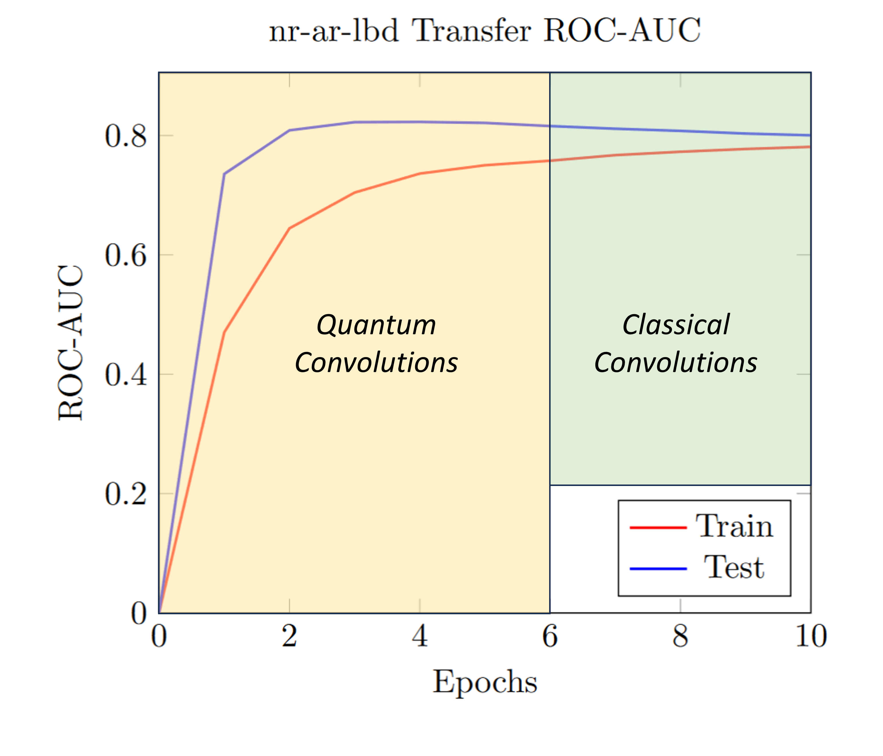
(d)

Figure S3: Training curves for the nr-ar-lbd assay

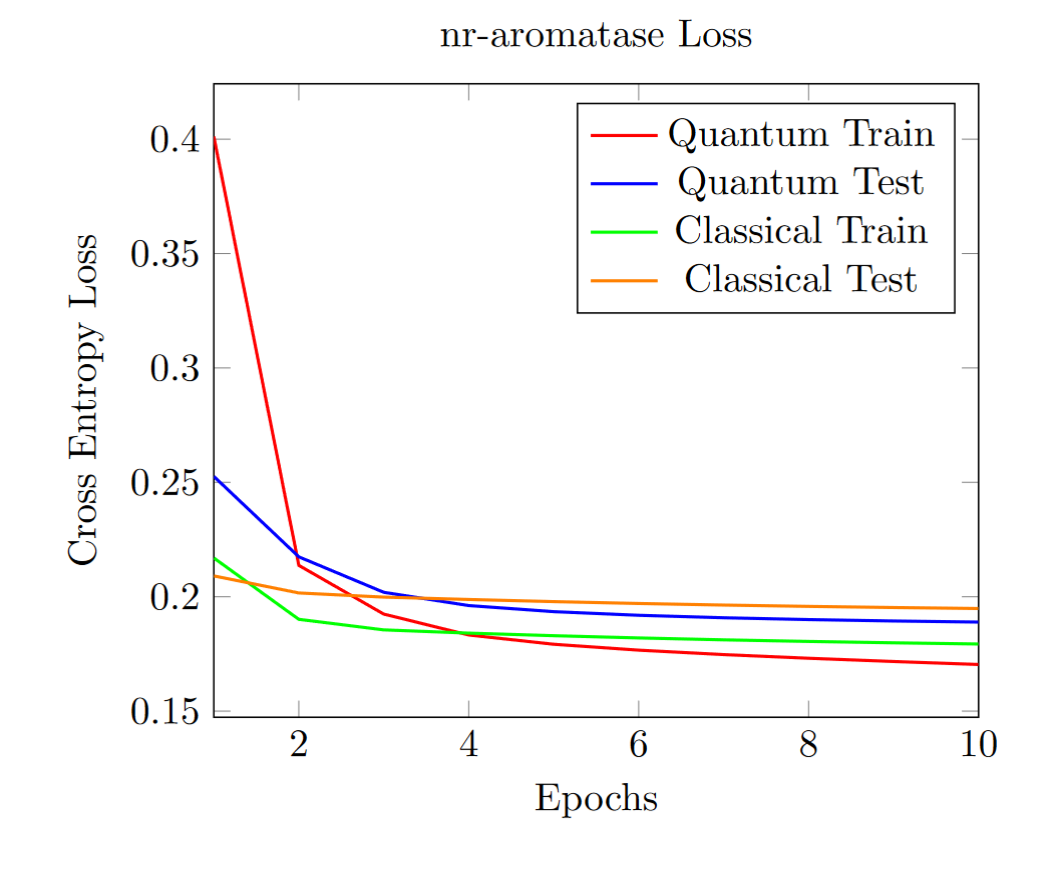
(a)

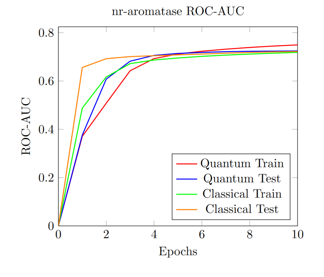
(b)

(c)

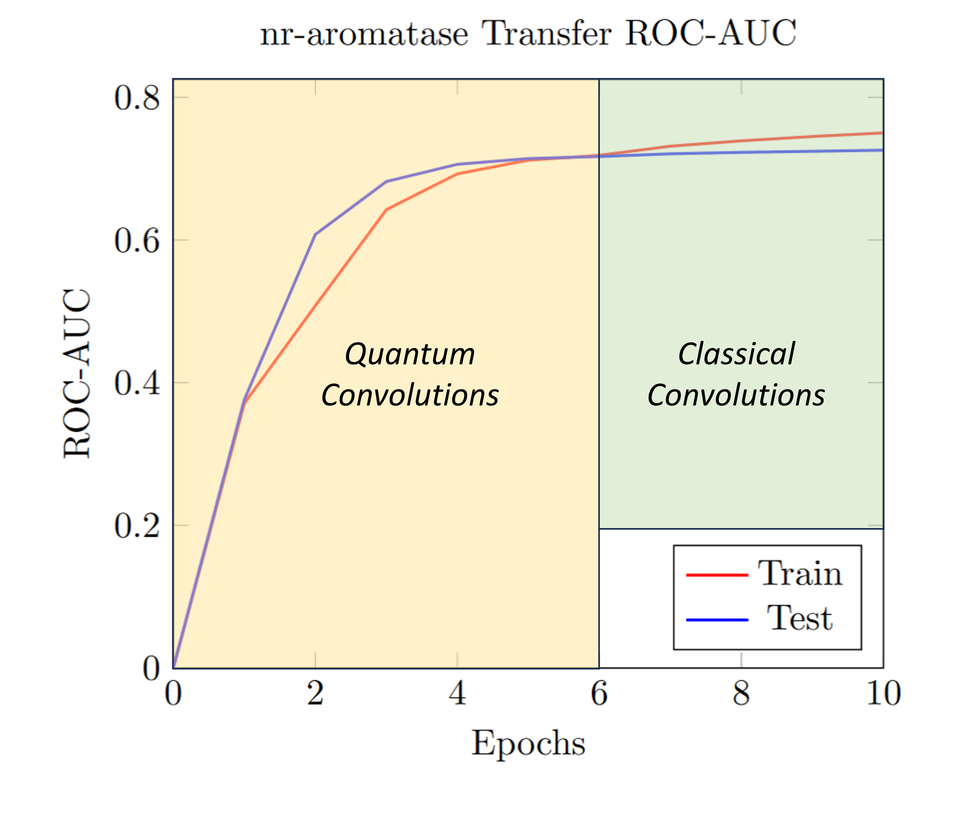
(d)

Figure S4: Training curves for the nr-aromatase assay

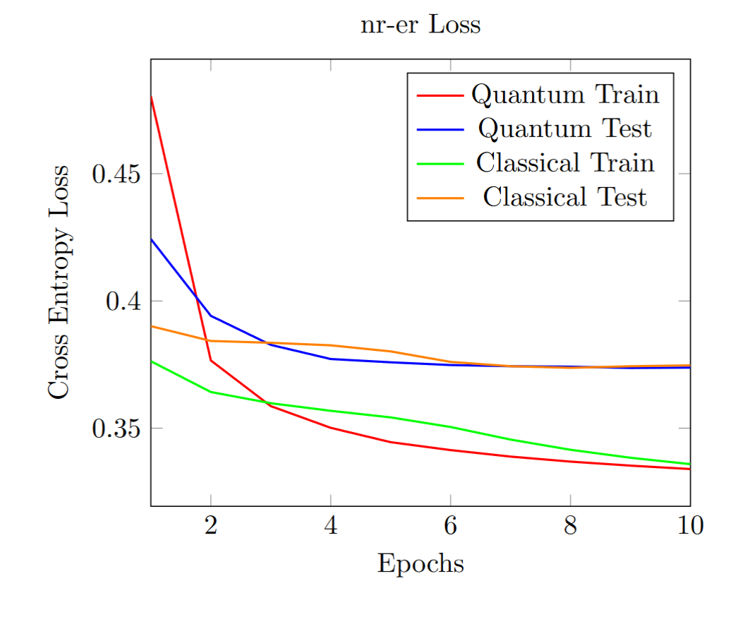
(a)

(b)

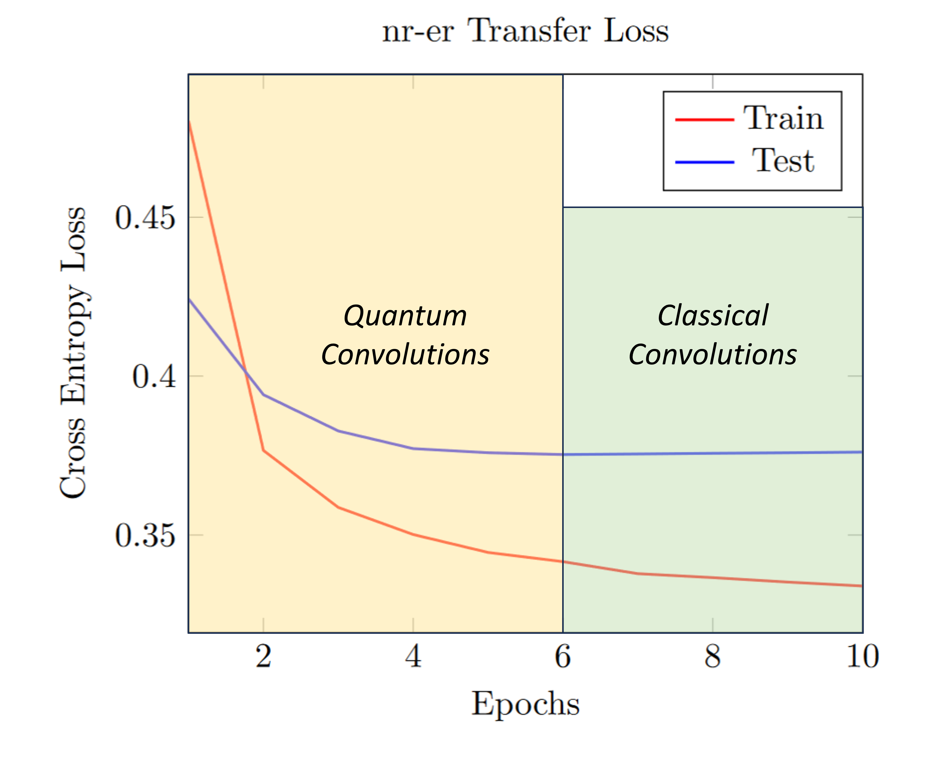
(c)

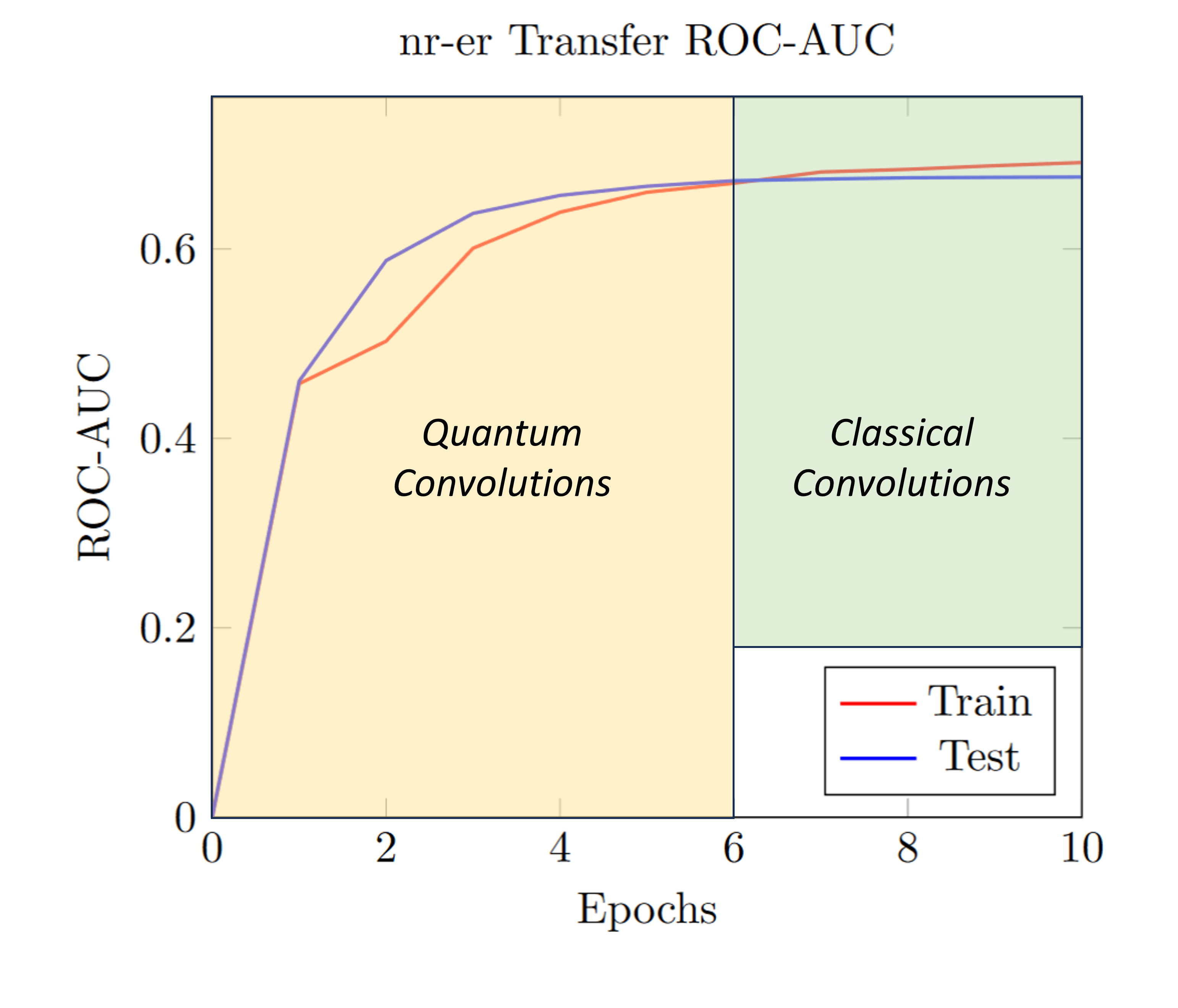
(d)

Figure S5: Training curves for the nr-er assay

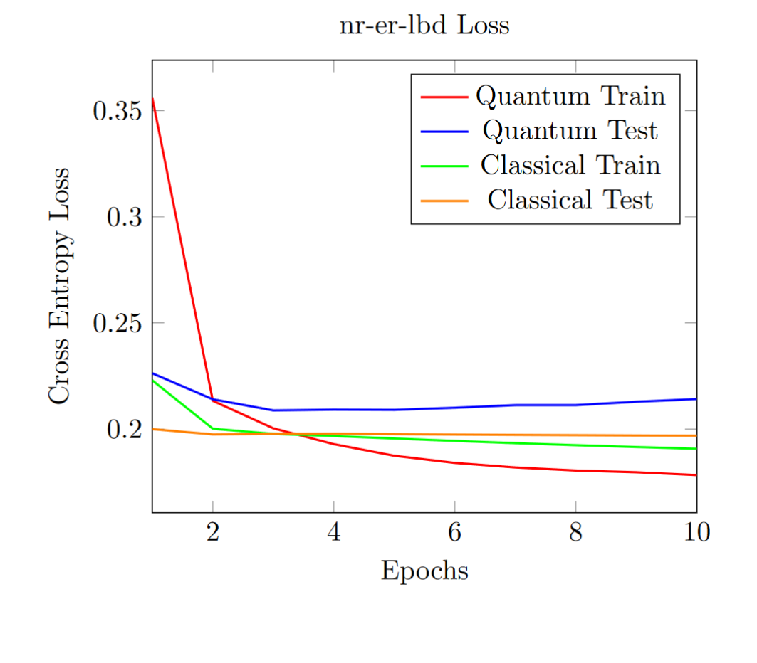
(a)

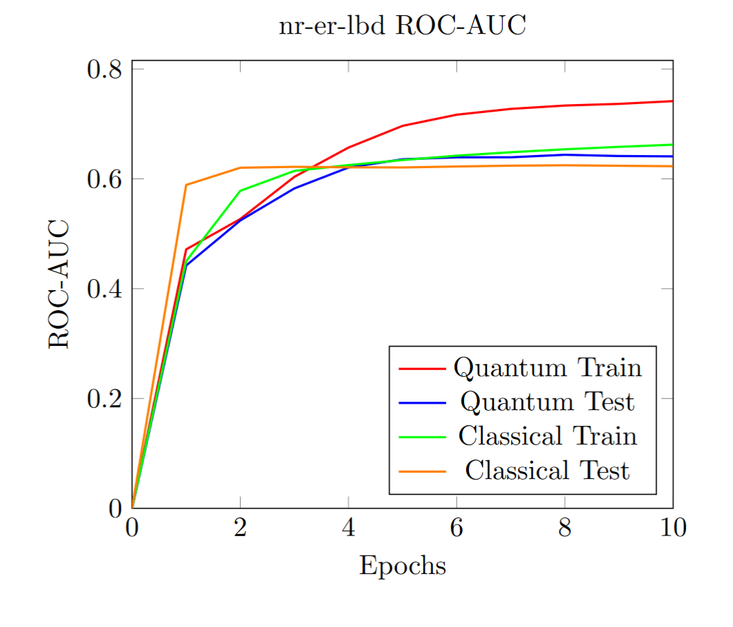
(b)

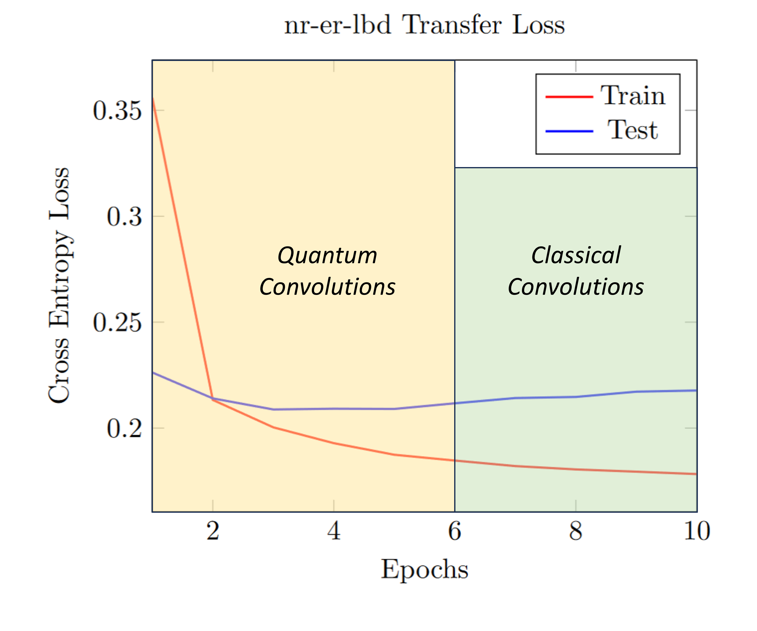
(c)

(d)

Figure S6: Training curves for the nr-er-lbd assay

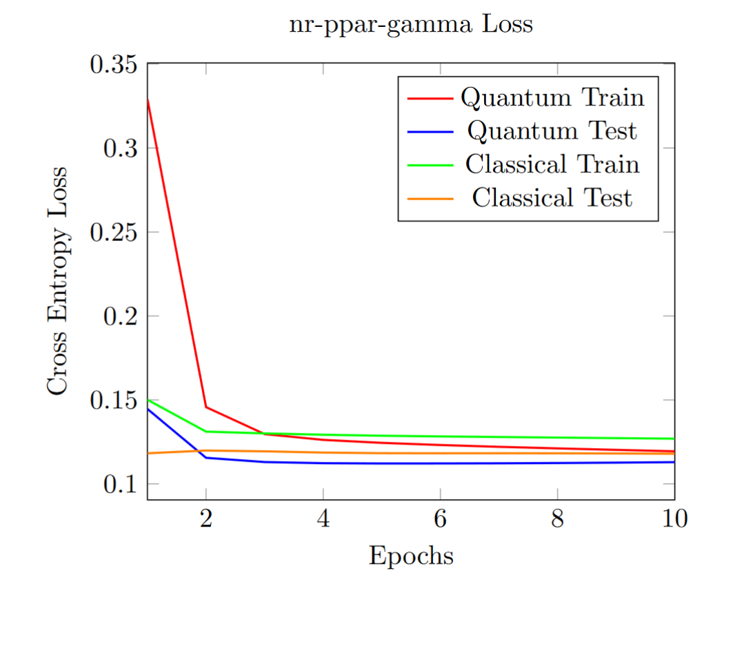
(a)

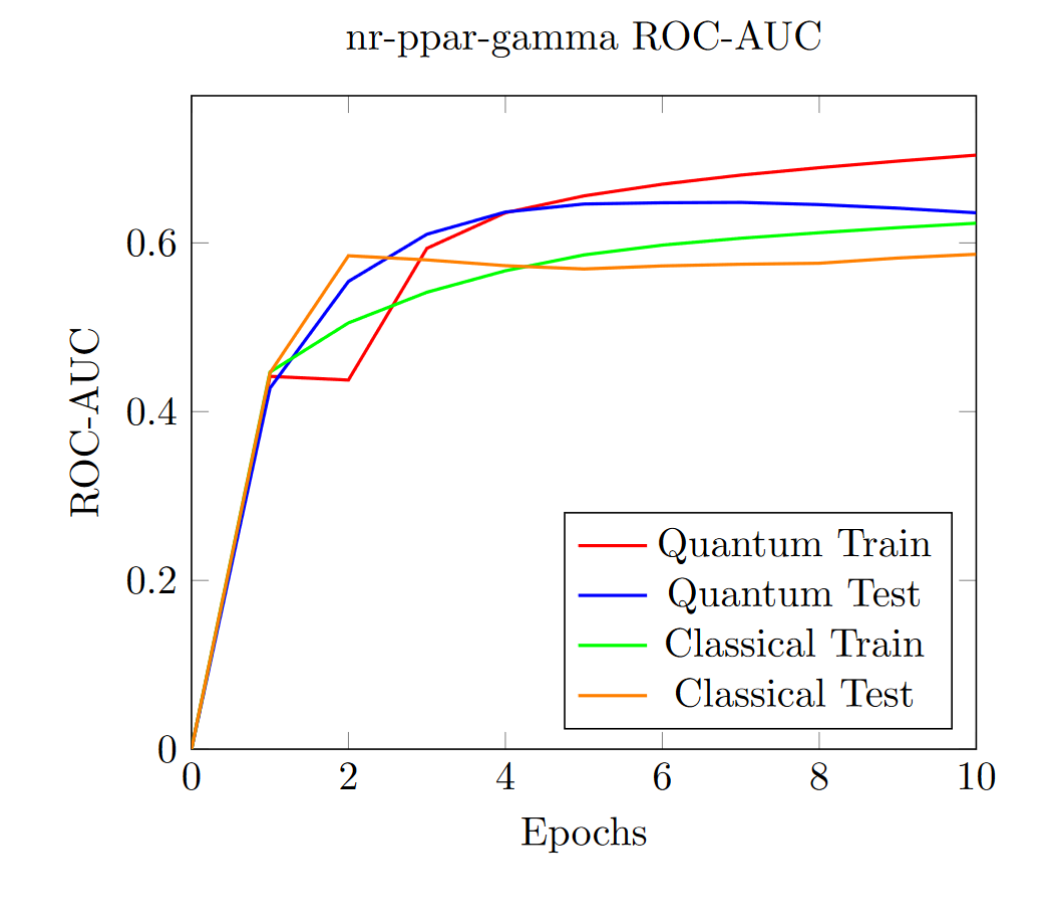
(b)

(c)

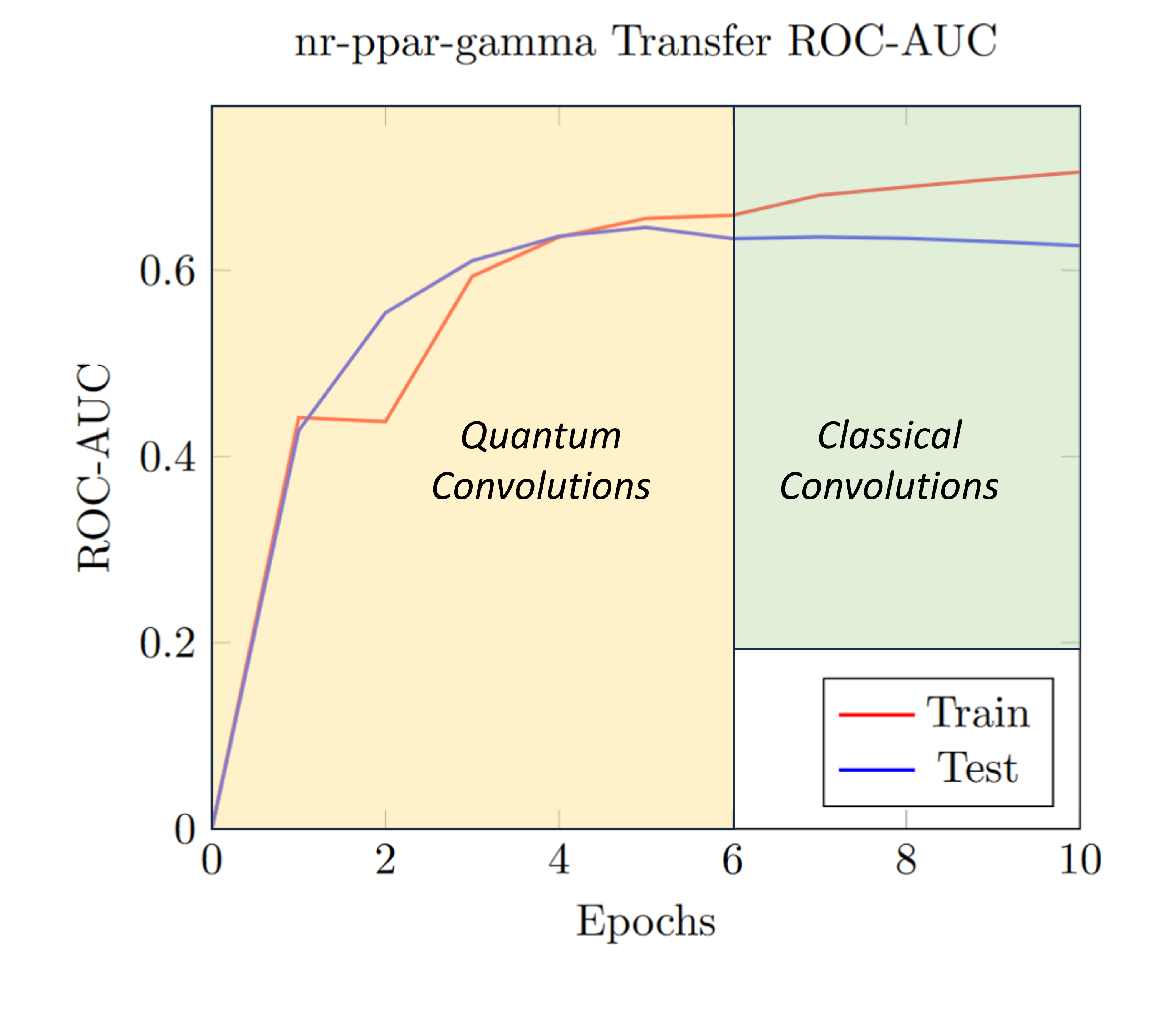
(d)

Figure S7: Training curves for the nr-ppar-gamma assay

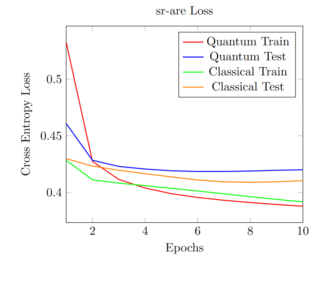
(a)

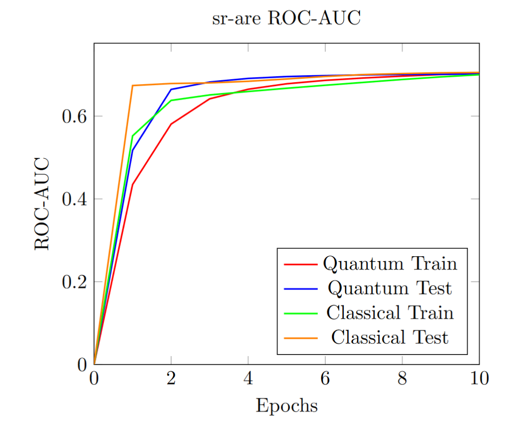
(b)

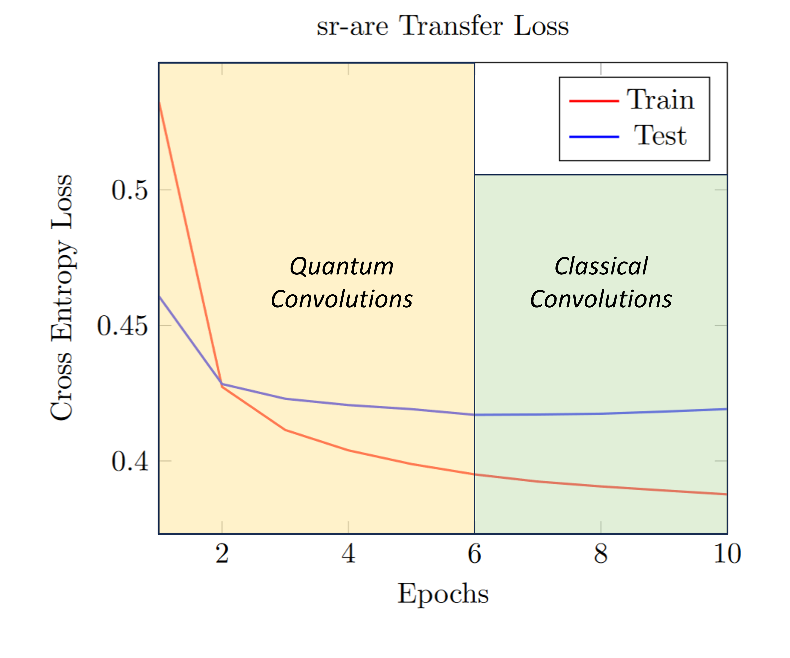
(c)

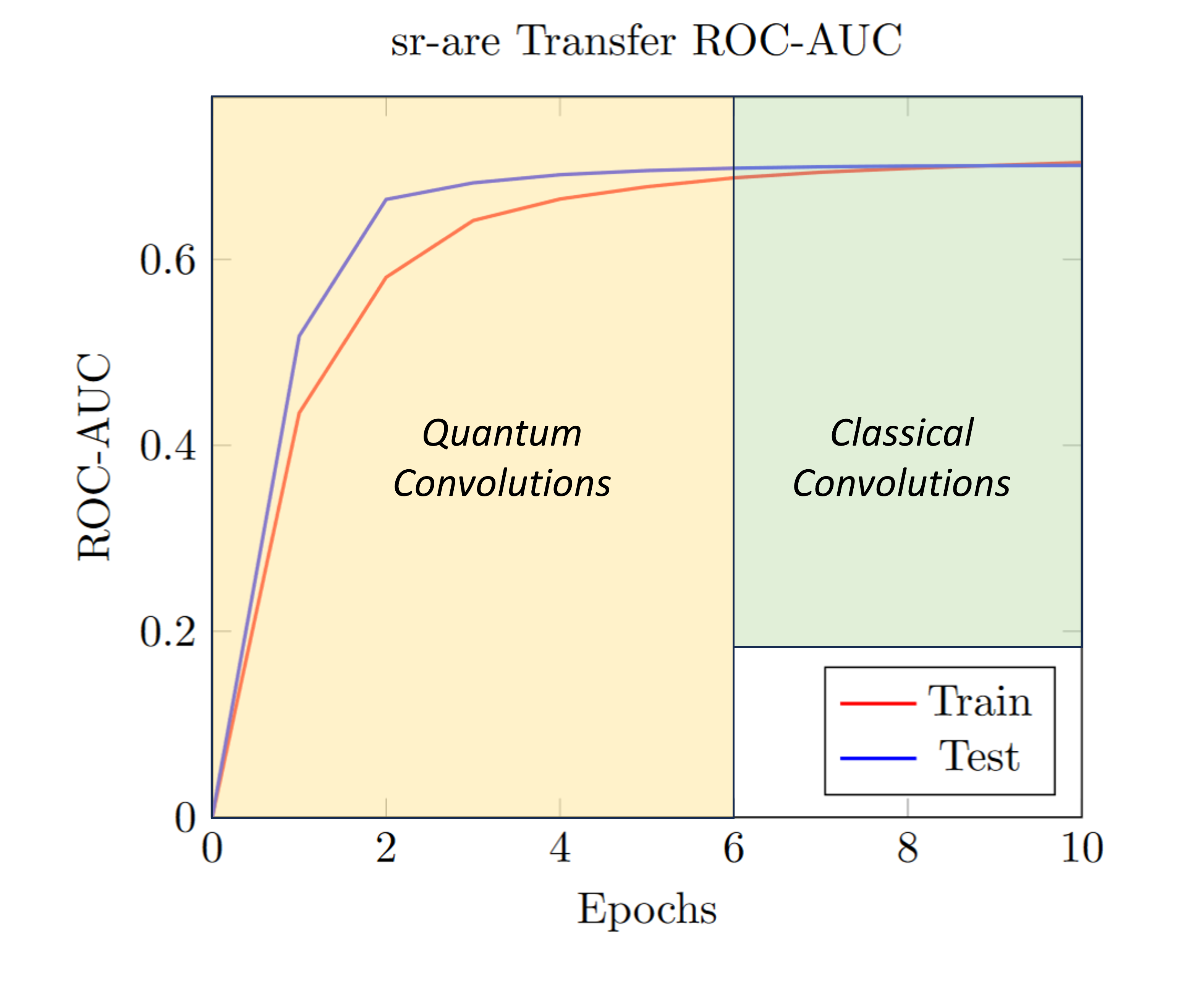
(d)

Figure S8: Training curves for the sr-are assay

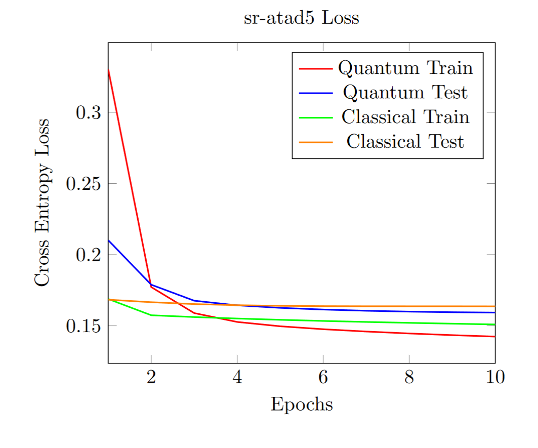
(a)

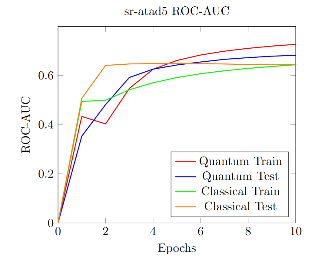
(b)

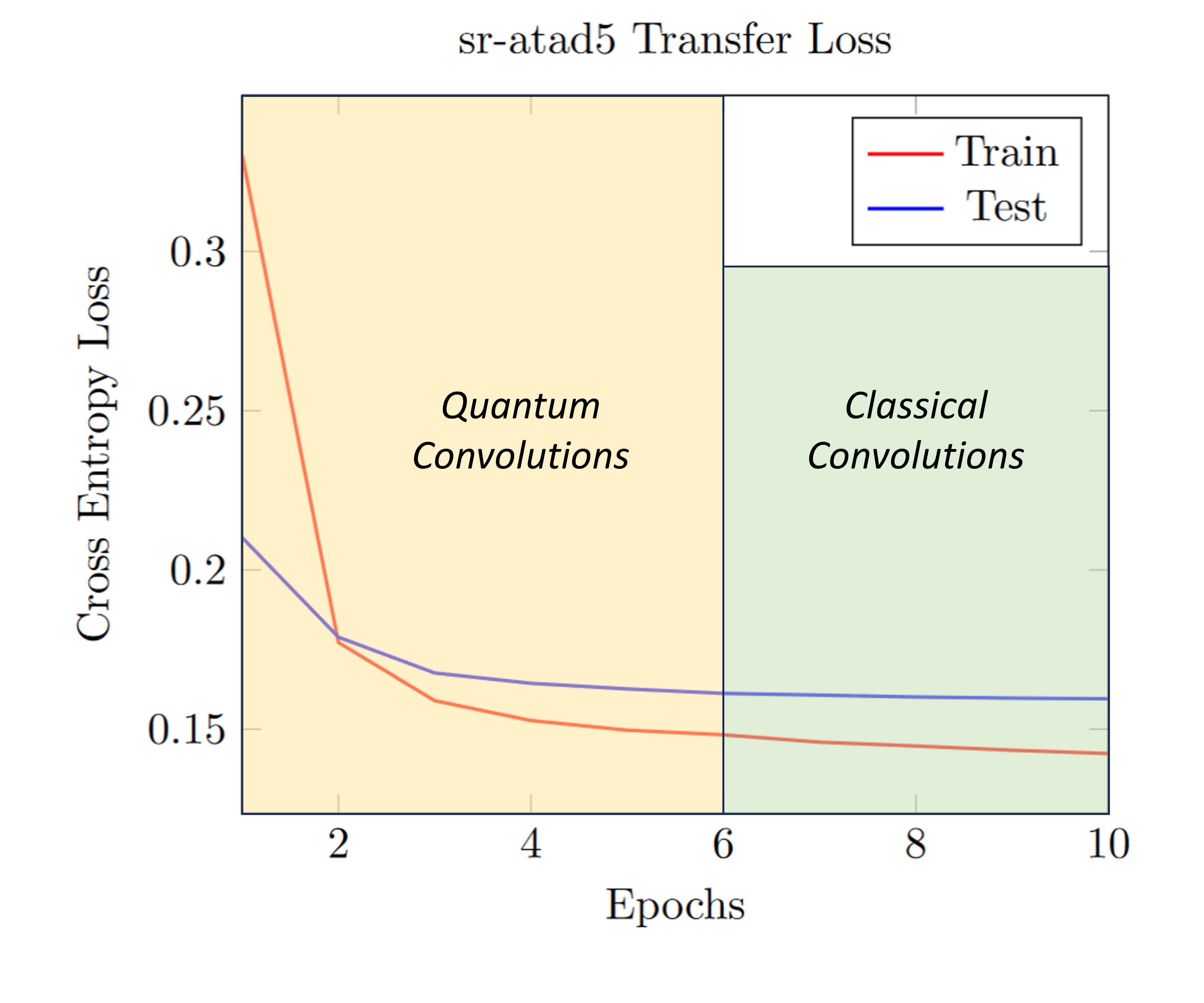
(c)

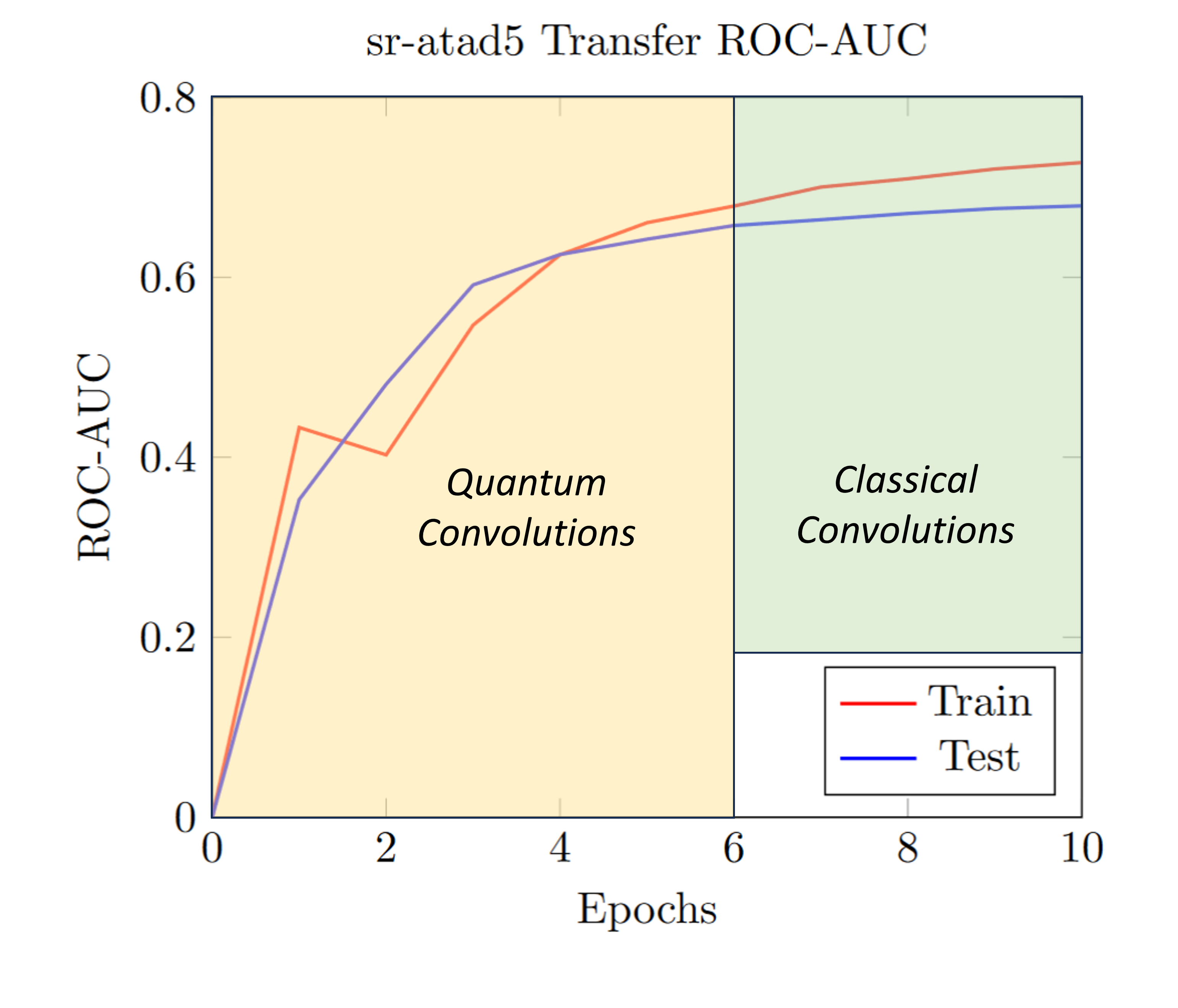
(d)

Figure S9: Training curves for the sr-atad5 assay

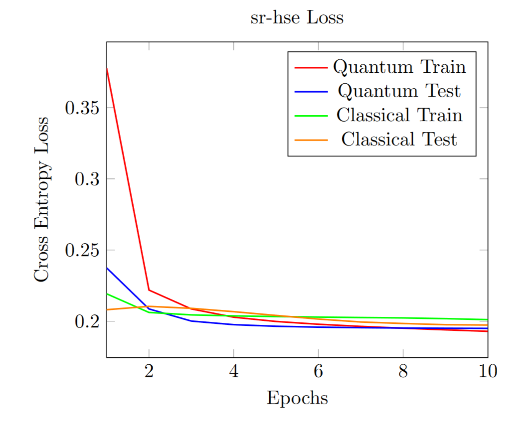
(a)

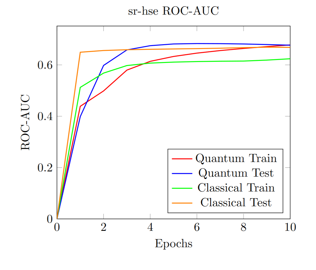
(b)

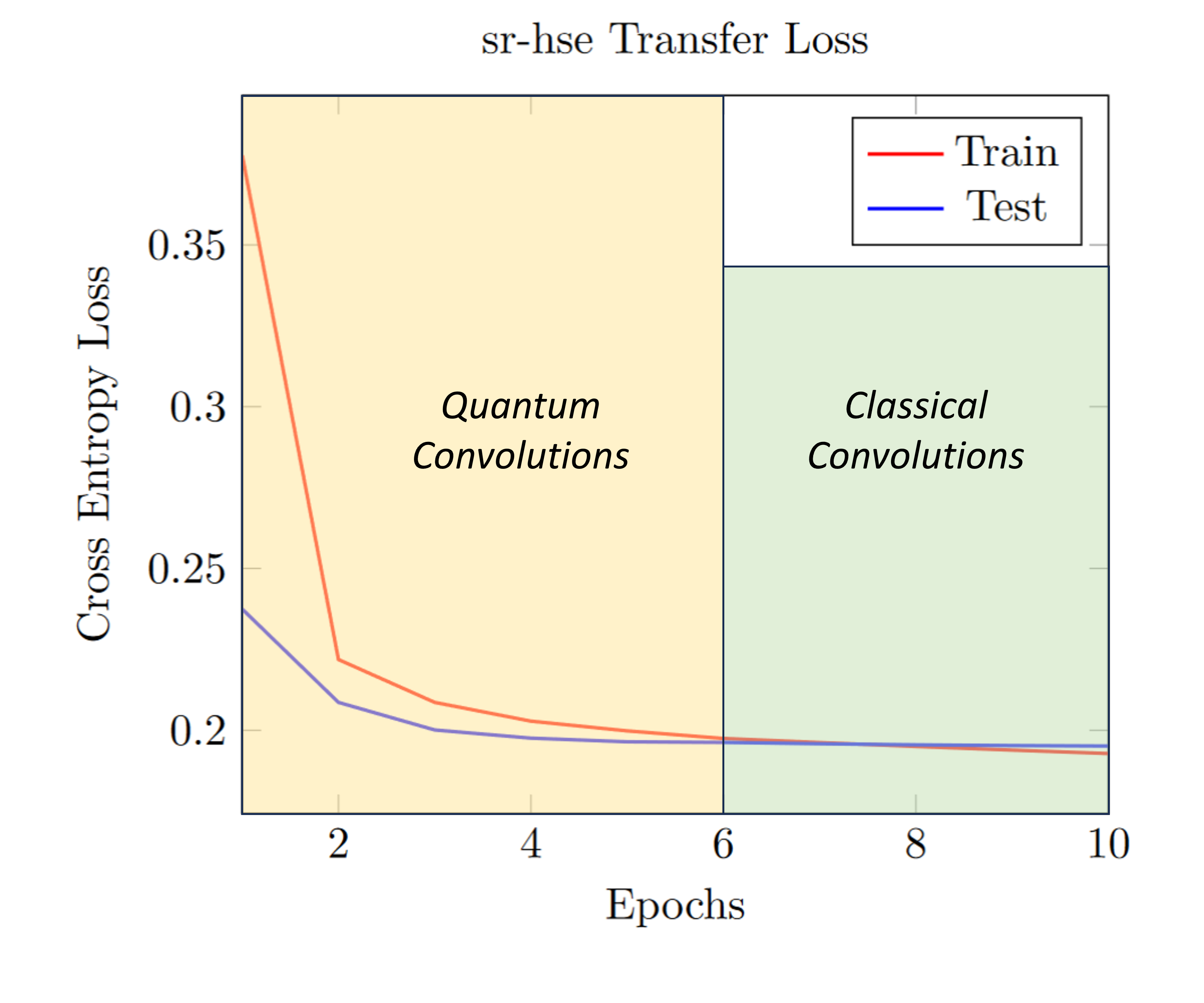
(c)

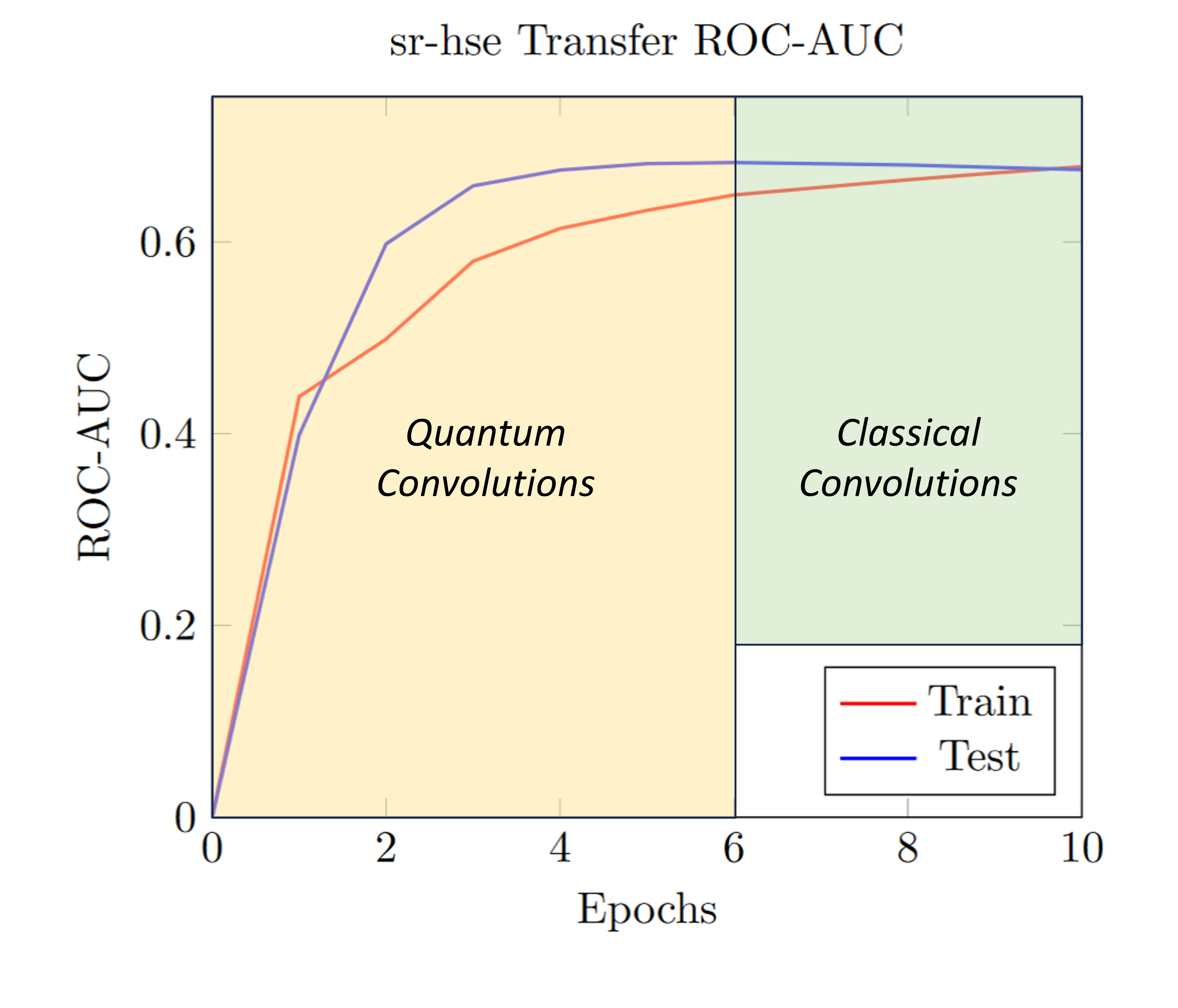
(d)

Figure S10: Training curves for the sr-hse assay

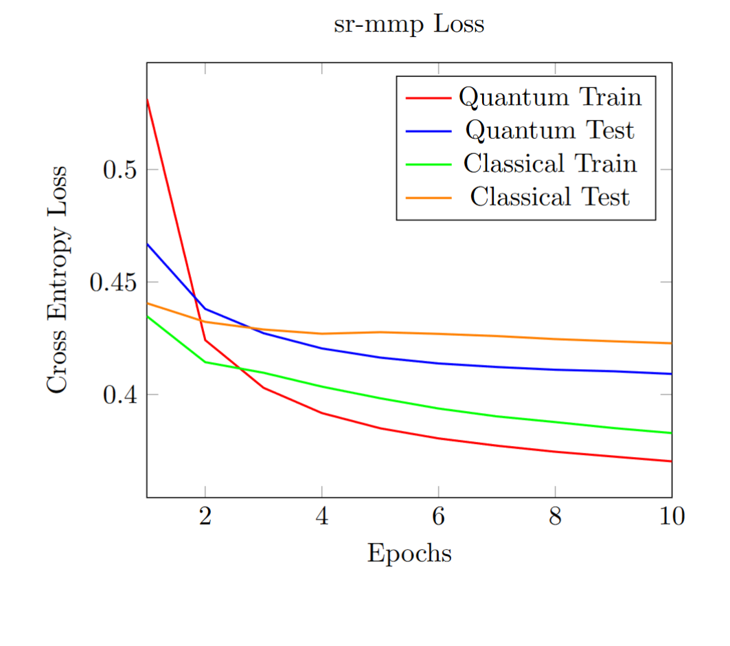
(a)

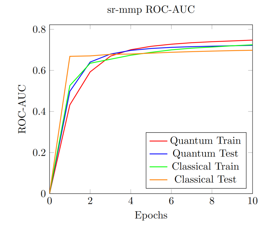
(b)

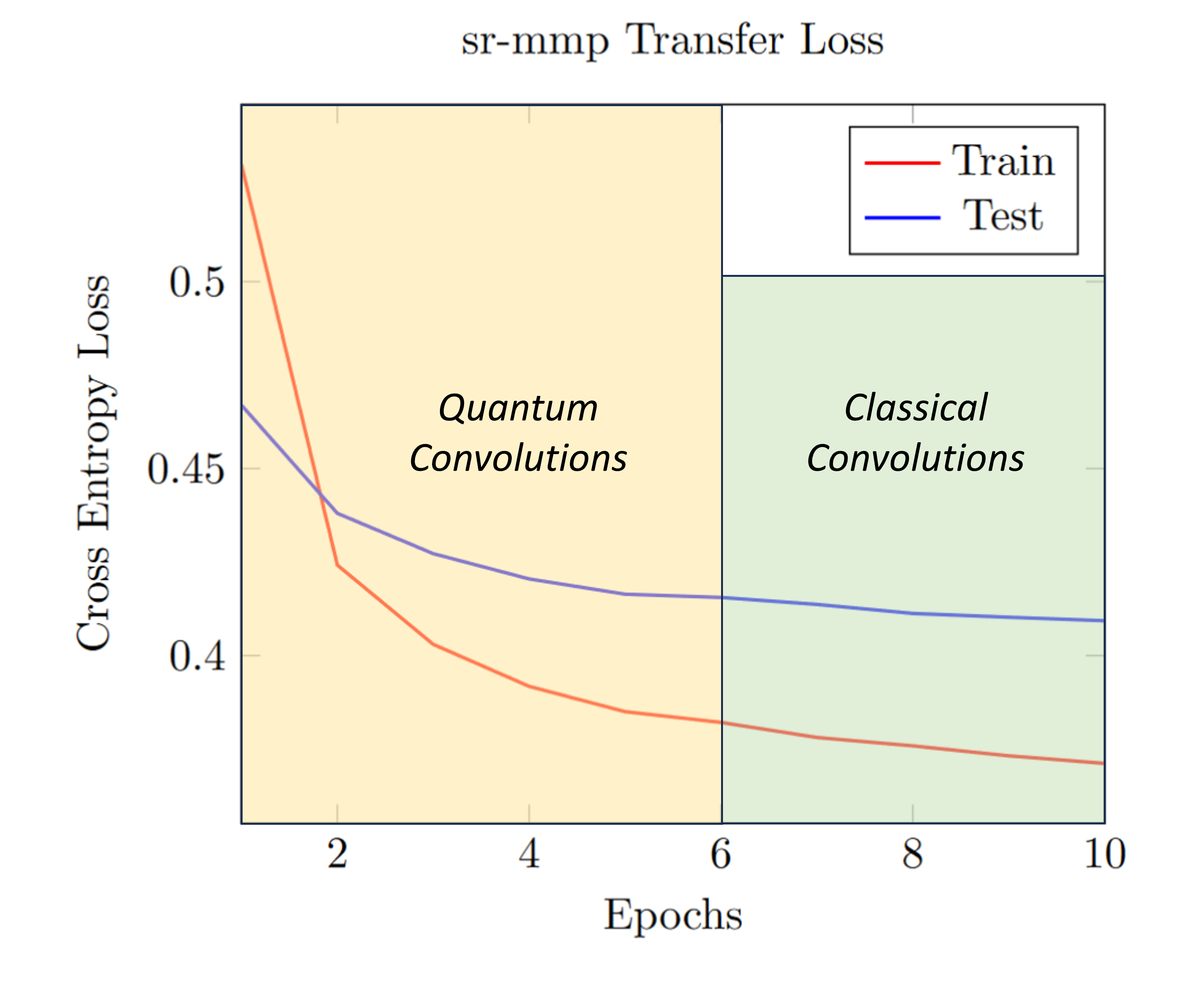
(c)

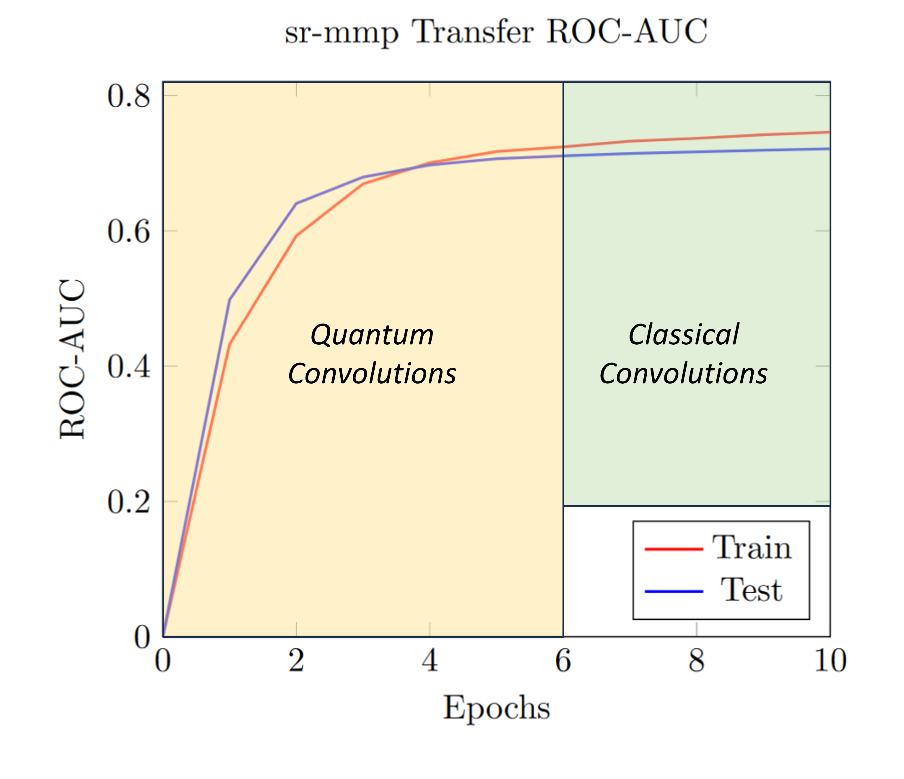
(d)

Figure S11: Training curves for the sr-mmp assay

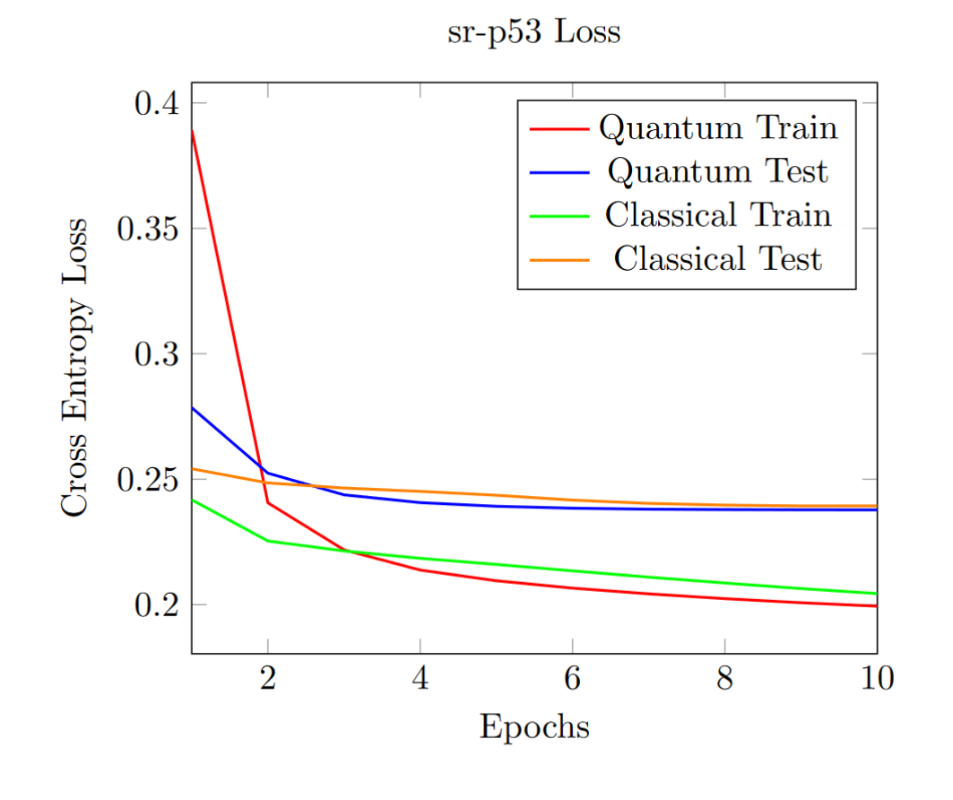
(a)

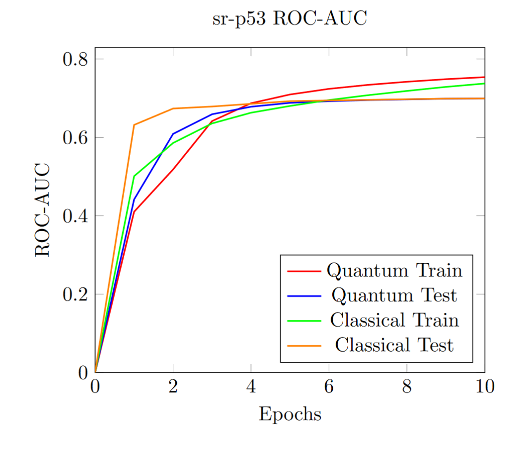
(b)

(c)

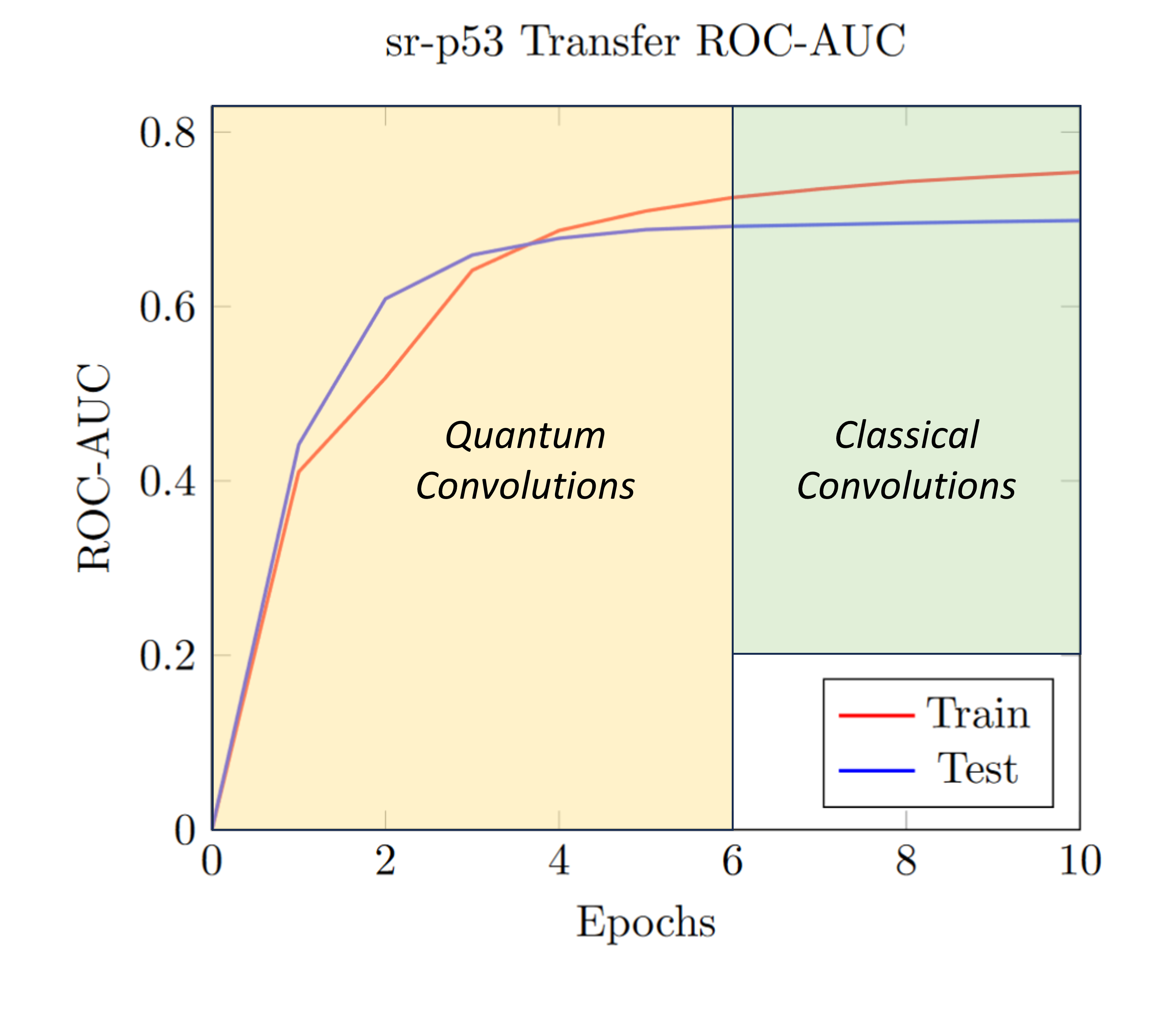
(d)

Figure S12: Training curves for the sr-p53 assay

References

- Sun et al. 2022 Sun, D.; Gao, W.; Hu, H.; Zhou, S. Why 90% of clinical drug development fails and how to improve it? Acta Pharmaceutica Sinica B 2022, 12, 3049–3062
- noa 2021 Research and Development in the Pharmaceutical Industry | Congressional Budget Office. 2021; https://www.cbo.gov/publication/57126
- Mullowney et al. 2023 Mullowney, M. W. et al. Artificial intelligence for natural product drug discovery. Nature Reviews Drug Discovery 2023, 22, 895–916
- Sarkar et al. 2023 Sarkar, C.; Das, B.; Rawat, V. S.; Wahlang, J. B.; Nongpiur, A.; Tiewsoh, I.; Lyngdoh, N. M.; Das, D.; Bidarolli, M.; Sony, H. T. Artificial Intelligence and Machine Learning Technology Driven Modern Drug Discovery and Development. International Journal of Molecular Sciences 2023, 24, 2026
- Volkamer et al. 2023 Volkamer, A.; Riniker, S.; Nittinger, E.; Lanini, J.; Grisoni, F.; Evertsson, E.; Rodríguez-Pérez, R.; Schneider, N. Machine learning for small molecule drug discovery in academia and industry. Artificial Intelligence in the Life Sciences 2023, 3, 100056
- Bian and Xie 2021 Bian, Y.; Xie, X.-Q. Generative chemistry: drug discovery with deep learning generative models. Journal of Molecular Modeling 2021, 27, 71
- Martinelli 2022 Martinelli, D. D. Generative machine learning for de novo drug discovery: A systematic review. Computers in Biology and Medicine 2022, 145, 105403
- Tang et al. 2021 Tang, B.; Ewalt, J.; Ng, H.-L. In Biophysical and Computational Tools in Drug Discovery; Saxena, A. K., Ed.; Topics in Medicinal Chemistry; Springer International Publishing: Cham, 2021; pp 221–243
- Semenova et al. 2020 Semenova, E.; Williams, D. P.; Afzal, A. M.; Lazic, S. E. A Bayesian neural network for toxicity prediction. Computational Toxicology 2020, 16, 100133
- Suzuki and Katouda 2020 Suzuki, T.; Katouda, M. Predicting toxicity by quantum machine learning. Journal of Physics Communications 2020, 4, 125012
- Mayr et al. 2016 Mayr, A.; Klambauer, G.; Unterthiner, T.; Hochreiter, S. DeepTox: Toxicity Prediction using Deep Learning. Frontiers in Environmental Science 2016, 3
- Nguyen et al. 2022 Nguyen, T.; Nguyen, G. T. T.; Nguyen, T.; Le, D.-H. Graph Convolutional Networks for Drug Response Prediction. IEEE/ACM Transactions on Computational Biology and Bioinformatics 2022, 19, 146–154
- Peng et al. 2020 Peng, Y.; Zhang, Z.; Jiang, Q.; Guan, J.; Zhou, S. TOP: A deep mixture representation learning method for boosting molecular toxicity prediction. Methods 2020, 179, 55–64
- Jiang et al. 2021 Jiang, J.; Wang, R.; Wei, G.-W. GGL-Tox: Geometric Graph Learning for Toxicity Prediction. Journal of Chemical Information and Modeling 2021, 61, 1691–1700
- Du et al. 2020 Du, Y.; Hsieh, M.-H.; Liu, T.; Tao, D. Expressive power of parametrized quantum circuits. Physical Review Research 2020, 2, 033125
- Du et al. 2021 Du, Y.; Hsieh, M.-H.; Liu, T.; Tao, D.; Liu, N. Quantum noise protects quantum classifiers against adversaries. Physical Review Research 2021, 3, 023153
- Du et al. 2021 Du, Y.; Hsieh, M.-H.; Liu, T.; You, S.; Tao, D. Learnability of Quantum Neural Networks. PRX Quantum 2021, 2, 040337
- Caro et al. 2022 Caro, M. C.; Huang, H.-Y.; Cerezo, M.; Sharma, K.; Sornborger, A.; Cincio, L.; Coles, P. J. Generalization in quantum machine learning from few training data. Nature Communications 2022, 13, 4919
- Gircha et al. 2023 Gircha, A. I.; Boev, A. S.; Avchaciov, K.; Fedichev, P. O.; Fedorov, A. K. Hybrid quantum-classical machine learning for generative chemistry and drug design. Scientific Reports 2023, 13, 8250
- Batra et al. 2021 Batra, K.; Zorn, K. M.; Foil, D. H.; Minerali, E.; Gawriljuk, V. O.; Lane, T. R.; Ekins, S. Quantum Machine Learning Algorithms for Drug Discovery Applications. Journal of Chemical Information and Modeling 2021, 61, 2641–2647
- Sajjan et al. 2022 Sajjan, M.; Li, J.; Selvarajan, R.; Hari Sureshbabu, S.; Suresh Kale, S.; Gupta, R.; Singh, V.; Kais, S. Quantum machine learning for chemistry and physics. Chemical Society Reviews 2022, 51, 6475–6573
- Mensa et al. 2023 Mensa, S.; Sahin, E.; Tacchino, F.; Barkoutsos, P. K.; Tavernelli, I. Quantum machine learning framework for virtual screening in drug discovery: a prospective quantum advantage. Machine Learning: Science and Technology 2023, 4, 015023
- Kao et al. 2023 Kao, P.-Y.; Yang, Y.-C.; Chiang, W.-Y.; Hsiao, J.-Y.; Cao, Y.; Aliper, A.; Ren, F.; Aspuru-Guzik, A.; Zhavoronkov, A.; Hsieh, M.-H.; Lin, Y.-C. Exploring the Advantages of Quantum Generative Adversarial Networks in Generative Chemistry. Journal of Chemical Information and Modeling 2023, 63, 3307–3318
- Domingo et al. 2023 Domingo, L.; Djukic, M.; Johnson, C.; Borondo, F. Binding affinity predictions with hybrid quantum-classical convolutional neural networks. Scientific Reports 2023, 13, 17951
- Banerjee et al. 2023 Banerjee, S.; Yuxun, S. H.; Konakanchi, S.; Ogunfowora, L.; Roy, S.; Selvaras, S.; Domingo, L.; Chehimi, M.; Djukic, M.; Johnson, C. A hybrid quantum-classical fusion neural network to improve protein-ligand binding affinity predictions for drug discovery. 2023; http://arxiv.org/abs/2309.03919, arXiv:2309.03919 [quant-ph]
- Dong et al. 2023 Dong, L.; Li, Y.; Liu, D.; Ji, Y.; Hu, B.; Shi, S.; Zhang, F.; Hu, J.; Qian, K.; Jin, X.; Wang, B. Prediction of Protein‐Ligand Binding Affinity by a Hybrid Quantum‐Classical Deep Learning Algorithm. Advanced Quantum Technologies 2023, 6, 2300107
- Vakili et al. 2024 Vakili, M. G. et al. Quantum Computing-Enhanced Algorithm Unveils Novel Inhibitors for KRAS. 2024; http://arxiv.org/abs/2402.08210, arXiv:2402.08210 [quant-ph]
- Hong et al. 2021 Hong, Z.; Wang, J.; Qu, X.; Zhu, X.; Liu, J.; Xiao, J. Quantum Convolutional Neural Network on Protein Distance Prediction. 2021 International Joint Conference on Neural Networks (IJCNN). 2021; pp 1–8, ISSN: 2161-4407
- Albrecht et al. 2023 Albrecht, B.; Dalyac, C.; Leclerc, L.; Ortiz-Gutiérrez, L.; Thabet, S.; D’Arcangelo, M.; Elfving, V. E.; Lassablière, L.; Silvério, H.; Ximenez, B.; Henry, L.-P.; Signoles, A.; Henriet, L. Quantum Feature Maps for Graph Machine Learning on a Neutral Atom Quantum Processor. Physical Review A 2023, 107, 042615, arXiv:2211.16337 [quant-ph]
- Bhatia et al. 2023 Bhatia, A. S.; Saggi, M. K.; Kais, S. Quantum Machine Learning Predicting ADME-Tox Properties in Drug Discovery. Journal of Chemical Information and Modeling 2023, 63, 6476–6486
- Villalobos et al. 2022 Villalobos, P.; Sevilla, J.; Besiroglu, T.; Heim, L.; Ho, A.; Hobbhahn, M. Machine Learning Model Sizes and the Parameter Gap. 2022; http://arxiv.org/abs/2207.02852, arXiv:2207.02852 [cs]
- Strassen 1969 Strassen, V. Gaussian elimination is not optimal. Numerische Mathematik 1969, 13, 354–356
- Williams et al. 2023 Williams, V. V.; Xu, Y.; Xu, Z.; Zhou, R. New Bounds for Matrix Multiplication: from Alpha to Omega. 2023; http://arxiv.org/abs/2307.07970, arXiv:2307.07970 [cs]
- Miller 1975 Miller, W. Computational Complexity and Numerical Stability. SIAM Journal on Computing 1975, 4, 97–107
- Shao 2018 Shao, C. A Quantum Model for Multilayer Perceptron. 2018; http://arxiv.org/abs/1808.10561, arXiv:1808.10561 [quant-ph]
- Stein et al. 2022 Stein, S. A.; Mao, Y.; Ang, J.; Li, A. QuCNN : A Quantum Convolutional Neural Network with Entanglement Based Backpropagation. 2022; http://arxiv.org/abs/2210.05443, arXiv:2210.05443 [quant-ph]
- Li and Wang 2020 Li, P.; Wang, B. Quantum neural networks model based on swap test and phase estimation. Neural Networks 2020, 130, 152–164
- Zhao et al. 2019 Zhao, J.; Zhang, Y.-H.; Shao, C.-P.; Wu, Y.-C.; Guo, G.-C.; Guo, G.-P. Building quantum neural networks based on a swap test. Physical Review A 2019, 100, 012334
- Shao 2018 Shao, C. Quantum Algorithms to Matrix Multiplication. 2018; http://arxiv.org/abs/1803.01601, arXiv:1803.01601 [quant-ph]
- Mari et al. 2020 Mari, A.; Bromley, T. R.; Izaac, J.; Schuld, M.; Killoran, N. Transfer learning in hybrid classical-quantum neural networks. Quantum 2020, 4, 340, arXiv:1912.08278 [quant-ph, stat]
- Kim et al. 2023 Kim, J.; Huh, J.; Park, D. K. Classical-to-quantum convolutional neural network transfer learning. Neurocomputing 2023, 555, 126643
- Schuman et al. 2023 Schuman, D.; Sünkel, L.; Altmann, P.; Stein, J.; Roch, C.; Gabor, T.; Linnhoff-Popien, C. Towards Transfer Learning for Large-Scale Image Classification Using Annealing-based Quantum Boltzmann Machines. 2023; http://arxiv.org/abs/2311.15966, arXiv:2311.15966 [quant-ph]
- Tice et al. 2013 Tice, R. R.; Austin, C. P.; Kavlock, R. J.; Bucher, J. R. Improving the human hazard characterization of chemicals: a Tox21 update. Environmental Health Perspectives 2013, 121, 756–765
- 44 National Institute of Health Tox21 Data Challenge 2014. https://tripod.nih.gov/tox21/challenge/data.jsp
- Buhrman et al. 2001 Buhrman, H.; Cleve, R.; Watrous, J.; de Wolf, R. Quantum Fingerprinting. Physical Review Letters 2001, 87, 167902
- Chen et al. 2020 Chen, J.; Cheong, H.-H.; Siu, S. W. I. BESTox: A Convolutional Neural Network Regression Model Based on Binary-Encoded SMILES for Acute Oral Toxicity Prediction of Chemical Compounds. Algorithms for Computational Biology 2020, 12099, 155–166
- Yuan et al. 2019 Yuan, Q.; Wei, Z.; Guan, X.; Jiang, M.; Wang, S.; Zhang, S.; Li, Z. Toxicity Prediction Method Based on Multi-Channel Convolutional Neural Network. Molecules 2019, 24, 3383
- Limbu et al. 2022 Limbu, S.; Zakka, C.; Dakshanamurthy, S. Predicting Dose-Range Chemical Toxicity using Novel Hybrid Deep Machine-Learning Method. Toxics 2022, 10, 706
- Cong et al. 2019 Cong, I.; Choi, S.; Lukin, M. D. Quantum convolutional neural networks. Nature Physics 2019, 15, 1273–1278
- Hur et al. 2022 Hur, T.; Kim, L.; Park, D. K. Quantum convolutional neural network for classical data classification. Quantum Machine Intelligence 2022, 4, 3
- Chen et al. 2022 Chen, S. Y.-C.; Wei, T.-C.; Zhang, C.; Yu, H.; Yoo, S. Quantum convolutional neural networks for high energy physics data analysis. Physical Review Research 2022, 4, 013231
- Herrmann et al. 2022 Herrmann, J. et al. Realizing quantum convolutional neural networks on a superconducting quantum processor to recognize quantum phases. Nature Communications 2022, 13, 4144
- Smaldone et al. 2023 Smaldone, A. M.; Kyro, G. W.; Batista, V. S. Quantum convolutional neural networks for multi-channel supervised learning. Quantum Machine Intelligence 2023, 5, 41
- Chawla et al. 2002 Chawla, N. V.; Bowyer, K. W.; Hall, L. O.; Kegelmeyer, W. P. SMOTE: Synthetic Minority Over-sampling Technique. Journal of Artificial Intelligence Research 2002, 16, 321–357
- de Veras et al. 2022 de Veras, T. M. L.; da Silva, L. D.; da Silva, A. J. Double sparse quantum state preparation. Quantum Information Processing 2022, 21, 204
- Gleinig and Hoefler 2021 Gleinig, N.; Hoefler, T. An Efficient Algorithm for Sparse Quantum State Preparation. 2021 58th ACM/IEEE Design Automation Conference (DAC). San Francisco, CA, USA, 2021; pp 433–438
- Bergholm et al. 2022 Bergholm, V. et al. PennyLane: Automatic differentiation of hybrid quantum-classical computations. 2022; http://arxiv.org/abs/1811.04968, arXiv:1811.04968 [physics, physics:quant-ph]
- Paszke et al. 2019 Paszke, A. et al. PyTorch: An Imperative Style, High-Performance Deep Learning Library. 2019; http://arxiv.org/abs/1912.01703, arXiv:1912.01703 [cs, stat]
- 59 CUDA Toolkit - Free Tools and Training. https://developer.nvidia.com/cuda-toolkit
- Kingma and Ba 2017 Kingma, D. P.; Ba, J. Adam: A Method for Stochastic Optimization. 2017; http://arxiv.org/abs/1412.6980, arXiv:1412.6980 [cs]
- Hanley and McNeil 1983 Hanley, J. A.; McNeil, B. J. A method of comparing the areas under receiver operating characteristic curves derived from the same cases. Radiology 1983, 148, 839–843
- Mottonen et al. 2004 Mottonen, M.; Vartiainen, J. J.; Bergholm, V.; Salomaa, M. M. Transformation of quantum states using uniformly controlled rotations. 2004; http://arxiv.org/abs/quant-ph/0407010, arXiv:quant-ph/0407010
- Schuld et al. 2020 Schuld, M.; Bocharov, A.; Svore, K.; Wiebe, N. Circuit-centric quantum classifiers. Physical Review A 2020, 101, 032308, arXiv:1804.00633 [quant-ph]