Homogenization and continuum limit of mechanical metamaterials
Abstract.
When used in bulk applications, mechanical metamaterials set forth a multiscale problem with many orders of magnitude in scale separation between the micro and macro scales. However, mechanical metamaterials fall outside conventional homogenization theory on account of the flexural, or bending, response of their members, including torsion. We show that homogenization theory, based on calculus of variations and notions of Gamma-convergence, can be extended to account for bending. The resulting homogenized metamaterials exhibit intrinsic generalized elasticity in the continuum limit. We illustrate these properties in specific examples including two-dimensional honeycomb and three-dimensional octet-truss metamaterials.
Dedicated to Alan Needleman, ab imo pectore, on the occasion of his 80th birthday.
1. Introduction
Mechanical metamaterials [1, 2, 3], or architected materials, are characterized by a reticular structure that affords great flexibility for tailoring and shaping their mechanical properties (cf., e. g., [4], for a review of stiffness, strength and damage tolerance; [5], for a review of fatigue performance; and [6], for a review of dynamic properties). Advances in fabrication techniques [2, 7, 8, 9] have brought within the realm of practicality new metamaterial designs that populate previously inaccessible areas of material-property space [10], including lightweight structures with high strength and elastic modulus [11, 12, 13, 14, 15, 16, 17, 18, 19, 1, 20]. Common designs include honeycomb structures [13, 20] and the octet-truss [21, 12, 13, 16, 17, 18, 19], among others [11, 13, 15, 22, 20, 23]. Metamaterials often exhibit scaling properties and size effects [24, 21] that exploit the “smaller is stronger” principle to beneficial effect, especially as regards fracture resistance [25, 26, 27, 28] and energy absorption [29].
Mechanical nanostructured metamaterials, when used in bulk applications, define a quintessential multiscale problem, with many orders of magnitude in scale separation between the micro and macro domains. Under such conditions, models—computational or otherwise—predicated on the explicit tracking of every individual member of the metamaterial are impractical and uncalled for, since locally, away from defects and stress concentrations, large numbers of members deform collectively under applied loading and jointly exhibit well-defined effective behavior that can be characterized by means of a continuum material law. Coarse-graining approaches [30, 31] based on the quasicontinuum method [32, 33, 34], data-driven approaches [35, 36, 37] and machine-learning approaches [38] have been proposed in order to bridge length scales while providing full-resolution of the lattice where necessary.
In this work, we seek to characterize analytically the effective behavior of metamaterials at the macroscale under conditions of strict separation between the structural and lattice scales. The identification of such effective material behavior is the aim of homogenization theory [39] and discrete-to-continuum techniques [40, 41]. However, mechanical metamaterials fall outside conventional homogenization theory on account of the flexural, or bending, response of their members.
We show that homogenization theory can be extended to account for bending and that the resulting homogenized metamaterials exhibit generalized elasticity of the micropolar type [42]. Such theories are often used to introduce an ad hoc micromechanical length into the material law (cf., e. g., [43] for a review and discussion). By contrast, in the present context the micropolar terms are physical and are introduced by bending. In addition, the form of the limiting continuum energy is identified uniquely and unequivocally by the homogenization analysis. We additionally show that, for linear-elastic matematerials, the effective moduli of the limiting continuum energy can be computed explicitly using the discrete Fourier transform. We illustrate these properties in specific examples including two-dimensional honeycomb and three-dimensional octet-truss metamaterials.
2. Mechanical metamaterials
We consider throughout open-cell mechanical metamaterials comprised of bars, possessing both axial and bending stiffness, connected at rigid joints capable of transmitting forces and moments.
2.1. Notational conventions
We denote by the set of integers; by the set of real numbers; and by the set of complex numbers.
The characteristic function of a subset is defined as
| (1) |
For a Lebesgue-measurable set , we denote by its Lebesgue measure, i. e., its length if ; its area if ; and its volume if .
We denote by the dot product of two vectors , ; by the tensor product of two vectors and , i. e., ; and by the product between a matrix and a vector . We use throughout the abbreviation
| (2) |
corresponding to assigning precedence to matrix multiplication over dot product. For a matrix we denote by its transpose and by
| (3) |
its symmetric and skewsymmetric parts.
Given two vectors and , we denote by the cartesian product of and , i. e., , for and , for . Given two points , , we denote by the segment of straight line joining the two points in .
Given a function , we denote by its partial derivative with respect to . For functions of one variable, we also write . We denote by the matrix of partial derivatives of , i. e., . Given a Lebesgue-measurable subset and an integrable function , we denote by
| (4) |
the Lebesgue integral of over .
2.2. Geometry of metamaterials
Mechanical metamaterials are locally periodic frame structures consisting of bars connected at a set of joints (cf., e. g., [4, 1]. Infinite metamaterials are comprised of types, or classes, of oriented bars, all the bars in a class being identical, including orientation, modulo translations. For instance, the bar classes of a honeycomb metamaterial are , or , Fig. 10. The local environment of a joint is the set of bars incident on the joint. Metamaterials contain different types, or classes, of local environments, all local environments in a class being identical modulo translations. Correspondingly, the joints of the metamaterial are classified into types, according to their local environment. For instance, the joint classes of a honeycomb metamaterial are , or , Fig. 10.
The joints and bars of an infinite metamaterial are embedded periodically in space so that joints and bars of the same class span shifted Bravais lattices. Thus, the positions of the joints in each class span a point set of the form
| (5) |
where is the dimension of space, e. g., for two-dimensional lattices and for three-dimensional lattices; is a basis of ; is a corresponding array of integer lattice coordinates; and are translation vectors, or shifts. We additionally denote by the volume of the unit cell of the spanning Bravais lattice of the metamaterial. The joints of a metamaterial can therefore be indexed by a pair , where designates the joint class and its lattice coordinate array.
A full description of an infinite metamaterial additionally requires a scheme for indexing its bars by type and position, and for tabulating their connections to joints. By periodicity and translation invariance, the bars of a given bar class span the same Bravais lattice as the joint classes, modulo translations. Thus, bars can be indexed by pairs , where designates the bar class and is a lattice coordinate array. In addition, an orientation of the bar classes identifies beginning and end joints in every bar, which we designate by the symbols , respectively (cf. Section 4 for examples).
The adjacency relations between bars and joints, or connectivity, can be defined by designating, for every bar , the corresponding beginning and end joints, and , respectively. We note that, by periodicity,
| (6) |
i. e., the adjacency relations are translation-invariant. The corresponding joint coordinates follow from (5) as
| (7) |
and the spanning vector of the joints follows as
| (8) |
which is independent of by the translation invariance property (6). We also denote by
| (9) |
the spanning segments of the bars, regarded as sets.
We refer to subsets of the infinite metamaterials just described as metastructures. The extent of a metastructure, i. e., its set of bars, may be characterized by means of an index set
| (10) |
For an infinite metamaterial, .
2.3. Elastic energy of metastructures
Within the framework of linearized kinematics, the joints of a metastructure are endowed with deflection and rotation-angle degrees of freedom, and , respectively. We further denote by
| (11) |
the set of degrees of freedom of joint . At the local level, we denote by
| (12) |
the set of local degrees of freedom of bar , where are the degree-of-freedom arrays of the joints of the bar.
The total energy of a linear-elastic metastructure of extent has the form
| (13) |
where is the elastic stiffness of a bar of class . Throughout this work, we consider straight bars of constant cross section. Other cases, such as bars in the form of curved beams, tapered beams, and others, can be treated likewise.
2.4. Straight two-dimensional beam of constant cross section
Two-dimensional metamaterials are characterized by planar geometries with joint coordinates , . In addition, we assume that the metamaterial remains planar after deformation, so that the joint degrees of freedom of the joints comprise in-plane deflections and a single rotation angle .
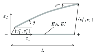
In order to represent the energy of the metamaterial, we consider a straight beam of length and constant cross section deforming in the -plane, in a reference configuration spanning the domain on the axis, Fig. 2. We denote by and the degrees of freedom of the beginning and end joint of the beam respectively. The corresponding linearized rotation matrices are
| (14) |
where denotes the Hodge-* operator. We additionally denote by the array of local degrees of freedom.
In this representation, an application of elementary beam theory [44] gives the energy of the beam as
| (15) |
where is the Young’s modulus of the beam, the cross-sectional area, the moment of inertia of the cross section, with principal axis of inertia perpendicular to the plane. The first term in (15) is the energy due to the axial deformation of the beam, whereas the second and third terms account for the energy due to bending.
The quadratic energy (15) can also be expressed in matrix form in terms of a stiffness matrix , whence the stiffness matrix of the bars of class in (13) follows as
| (16) |
in terms of some suitable, class-dependent, orthonormal change-of-axes matrix .
By direct inspection of (15), we verify that the global energy (13) is material-frame indifferent, i. e., invariant under transformations of the form
| (17a) | |||
| (17b) | |||
where represents a rigid linearized rotation and a rigid translation in the plane.
From these properties, the global energy (13) follows directly in global coordinates as
| (18) |
where we write
| (19a) | |||
| (19b) | |||
| (19c) | |||
and
| (20) |
are orthonormal directors for each bar class, with a unit vector aligned with the oriented axis and a unit vector perpendicular to with orientation chosen such that defines a right-handed orthonormal basis. The variables
| (21a) | |||
| (21b) | |||
in (18) may be interpreted as local axial and bending strains, the first and second terms in (18) then supplying the corresponding axial and bending energies, respectively.
2.5. Straight three-dimensional beam of constant cross section
Three-dimensional metamaterials are characterized by spatial geometries with joint coordinates , , and joint degrees of freedom comprising deflections and rotation angles . With this parametrization, the corresponding linearized rotation matrices are
| (22d) | |||
| (22e) | |||
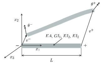
where we use the Hodge-* operator. With as the array of local degrees of freedom, elementary beam theory [44] now gives the energy of the beam as
| (23) |
where its cross-sectional area, its torsional moment of inertia, and its principal moments of inertia about axes and , respectively, is the Young’s modulus and is the shear modulus.
As in the two-dimensional case, the quadratic energy (23) can be expressed in matrix form in terms of a stiffness matrix , and the stiffness matrices of the bars of class in cf. (13) then follow as in (16) in terms of orthonormal transformation matrices . The resulting global energy (13) is again material-frame-indifferent, i. e., invariant under transformations of the form (17), with now representing a rigid linearized rotation and a rigid translation in three-dimensional space.
Alternatively, from these properties the global energy (13) follows directly in global coordinates as
| (24) |
where , and are as in (19) and is an orthonormal director triad in which is the direction of the bar axis, eq. (20), and and are the principal directions of inertia of the cross section.
As in the two-dimensional case, the variables
| (25a) | |||
| (25b) | |||
may be interpreted as local axial and bending strains, the axial and bending energies in (24) then being quadratic in the corresponding strains.
3. The continuum limit of metamaterials
Next, we concern ourselves with the limit in which the metamaterial cell-size is much smaller than the domain size, or continuum limit. To this end, we appeal to tools from calculus of variations, especially methods of -convergence [45], as they bear on discrete-to-continuum problems [46, 41]. The fundamental property of variational methods is that they ensure convergence of the solutions of the finite cell-size problem to the solutions of the limiting continuum model. However, we note that the local energy of the bars in (18) and (24) includes terms that penalize the difference between the deflection-compatible rotations and the mean rotations of the bars, e. g., and in (18) and similar terms in (24), respectively. This local energy structure renders the attendant homogenization analysis non-standard and outside the scope of conventional discrete-to-continuum results (cf. [46, 41].
In order to characterize the continuum limit, we consider throughout metastructures whose extent is defined by a domain . Specifically, the metastructure maximally contained in is defined by the index set
| (26) |
with as in (7) and as in (9). Thus, (26) records all the bars that are fully contained in . It also supplies a criterion for terminating the metastructure at the boundary. We additionally denote by the index set of the joints in the metastructure, i. e.,
| (27) |
Henceforth, we denote by the energy (24) of the metastructure maximally contained within . For ease of handling, we decompose the energy as
| (28) |
in terms of an axial energy
| (29) |
a bending energy,
| (30) |
and a coupling energy
| (31) |
3.1. Integral representation of the energy
In order to facilitate the passage to the continuum and make contact with homogenization theory [39] , we rewrite the energy (28) in integral form. To this end, we introduce a number of auxiliary structures.
Let be the Voronoi cell of bar in an infinite metamaterial, i. e.,
| (32) |
i. e., is the locus of points that are closer to be bar than to any other bar in the metamaterial. The measure
| (33) |
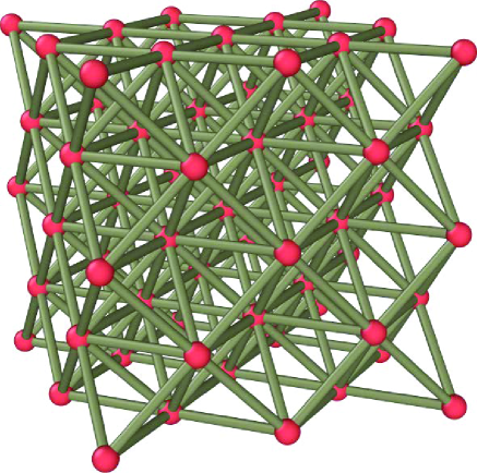
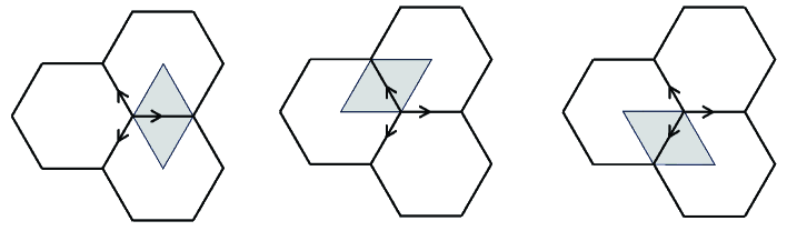
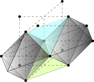
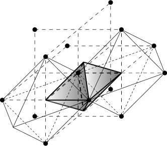
does not depend on by periodicity and translation invariance. Figs. 4 and 5 depict examples of Voronoi cells for a two-dimensional honeycomb structure and a three-dimensional octet-truss, respectively, by way of illustration.
We note that the bar domains are polygons, for , and polyhedra, for , consisting of simplices incident on the spanning segment of the bar, cf. Figs. 4 and 5. We denote by the collection of all such simplices, which together constitute a triangulation of . We note that the vertex set of includes—but its larger than—the set of joints of the metamaterial.
Consider now a metastructure maximally contained in . We denote by the restriction of to . Precisely, is the union of the Voronoi cells of all bars . We denote by the domain spanned by . By this construction, is a triangulation of . However, in general, though the discrepancy is rendered small upon scaling, in a sense to be made precise.
Let be a displacement of the metastructure and a piecewise linear function, not renamed, supported on the triangulation , such that
| (34) |
Then, is a piecewise constant function also supported on the triangulation .
We remark that the function is not uniquely defined by the discrete variables , as additional degrees of freedom arise at corners of the Voronoi cells which do not correspond to joints. The value of at these degrees of freedom can be fixed, for example, by minimizing the mean square oscillation of inside each cell of the metastructure, thus rendering the definition unique. In the case of simplicial metamaterials, as for example triangular metamaterials in two dimensions, can be made constant on each cell of the metastructure.
Using the identity
| (35) |
and the piecewise-constant property of , we obtain
| (36) |
Introducing the piecewise-constant axial moduli
| (37) |
with as in (1) and coefficients
| (38) |
the axial energy (36) further reduces to the integral form
| (39) |
We note that the inhomogeneous moduli thus defined are periodic with the periodicity of the metamaterial.
Proceeding likewise, we arrive at the integral form of the bending energy
| (40) |
where
| (41) |
are piecewise-constant bending moduli with coefficients
| (42) |
Finally, we turn to the coupling energy. As before, let be a displacement of the metastructure. In contrast to the fully conforming interpolation used in the foregoing, we now let be a piecewise linear function and a piecewise constant function, not renamed, both supported on the triangulation , and such that
| (43a) | ||||
| (43b) | ||||
As before, is a piecewise constant function supported on . Using again the identity (35) and the piecewise-constant property of , we obtain
| (44) |
Equivalently, we have
| (45) |
in terms of the Hodge-* operators (14) and (22). Introducing the piecewise-constant coupling moduli
| (46) |
with coefficients
| (47) |
the coupling energy (45) reduces to the integral form
| (48) |
which penalizes differences between the deflection-compatible rotations and the mean rotations of the bars. We again note that the inhomogeneous moduli thus defined are periodic with the periodicity of the metamaterial.
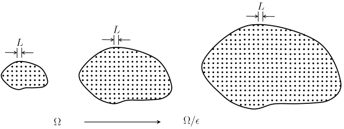
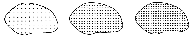
3.2. Scaling
Next, we consider a sequence of metastructures composed of the same metamaterial but spanning increasingly larger self-similar domains , where is a small scaling factor, Fig. 6. The corresponding metastructure is defined by the index set
| (49) |
Note that, in this scaling, the geometry of the metamaterial at the unit-cell scale as well and the material properties and the geometry of the cross sections of the bars, remain unchanged along the sequence. In particular, the bar lengths , cross-sectional areas and moments of inertia are not scaled according to . By contrast, the number of bars in the metastructure grows as and the metastructure spans an infinite metamaterial in the infinite body limit .
With , we consider the sequence of energy functions
| (50) |
where the factor accounts for the expected elasticity scaling of the limiting energy and is included to ensure a proper limit.
From (39), (40) and (48), we have the identity
| (51) |
for displacement fields in the class of piecewise-linear or piecewise-constant functions supported on defined in Section 3.1.
The structure of (51) is noteworthy. Thus, the energy consists of three terms: an axial energy; a bending energy, including torsion; and a coupling energy that couples deflection-compatible rotations and free rotations. Energies of the form (51) were termed micropolar by [42] and set forth an example of a theory of generalized continua. Such theories are often used to introduce an ad hoc micromechanical length into the material law that renders the energy non-local, in an effort to account for size effects. By contrast, in the present context the micropolar terms are physical and introduced into the energy by bending.
Rescaling the domain back to , Fig. 7, by means of the change of variables and rescaling of the variables
| (52) |
(51) becomes
| (53) |
where we have dropped the prime for simplicity and the new displacement fields are in the class of piecewise-linear or piecewise-constant functions supported on the scaled triangulation .
3.3. Continuum limit
We wish to ascertain the asymptotic behavior of the forced energy-minimizing configurations of the discrete energies (53) as , or continuum limit. Specifically, we wish to determine whether a continuum limiting energy exists with the property that the sequence of minimum discrete potential energies converges to the minimum continuum potential energy for all admissible forcings. Then, we say that is the variational limit, or -limit, of the sequence [45]).
Thus, suppose that the metastructure is acted upon by macroscopic distributed actions defined by the functions
| (54) |
where and are distributed forces and moments, or torques, per unit volume, respectively. The work of the applied actions is then
| (55) |
where is the volume of the unit cell of the spanning Bravais lattice of the metamaterial and the factor represents the volume per joint class. Its value follows from the property that all joint classes have the same number of joints per unit volume, or joint density.
Consider now a sequence of scaled energies defined in (53). Assume now that the sequence of energies is uniformly stable, or equicoercive. Specifically, we assume that there is a constant such that
| (56) |
for some suitable energy norm . This equicoercivity condition expresses the property that is bounded below for all by a structurally stable quadratic energy, i. e., a positive quadratic energy devoid of zero-energy modes. This property effectively prevents the emergence of finely oscillating unstable modes that corrupt the solution, at no cost in energy, as .
The norm entering (56) needs to be chosen carefully, and a suitable choice may not be immediately apparent for some metastructures. First, the metamaterial needs to be appropriately truncated at the boundary, eliminating for example dangling bonds from the domain on which is computed. Second, the norm needs to be strong enough to ensure continuity of the energy up to boundary terms. Third, the ancillary degrees of freedom need to be eliminated as discussed after (34), and the resulting metamaterial needs to be sufficiently rigid to provide coercivity. For example, for a triangular metamaterial in two dimensions, the axial energy immediately provides control of the norm of the strain , which leads to control of and via Korn’s inequality and appropriate boundary data. Using this property, the coupling energy gives control of , and finally the bending energy gives control of . The situation for the honeycomb lattice is more complex, as mechanisms exist for the axial energy, which correspond to zero-axial-energy deformations in addition to rigid-body motions. These zero-energy modes need to be stabilized by the bending and coupling energies in the long-wavelength limit relevant to the macroscopic material behavior.
With these provisos, the equilibrium configuration of the metastructure then follows by minimizing the potential energy
| (57) |
Denote by the corresponding minimum potential energy. Then, the variational limit, or -limit, of the sequence is characterized by the property that
| (58) |
for all admissible forcings , where is the minimum of the limiting potential energy
| (59) |
(cf., e. g., [45, Theorem 13.5, Corollary 13.7]). Variational convergence, together with the equicoercivity condition (56), in turn ensures the weak convergence of the sequence of minimizers to the minimizer of for all admissible forcings .
In view of the structure of the energy (28), the corresponding variational limit as extends variational discrete-to-continuum problems [41, 46] to account for bending. Alternatively, appealing to the density of piecewise linear and constant displacements over the increasingly finer triangulations , the energy (53) can be extended (by infinity) to continuum displacement fields without altering the continuum limit. The resulting limiting problem then falls within the class of variational homogenization problems (cf., e. g., [39]).
In addition, in view of the factor in (53) we expect the bending energy to be negligible in the limit, and the limiting continuum energy to be of the form
| (60) |
for some effective energy density , to be determined, and for a certain class of sufficiently regular and finite domains . In particular, the effective energy density is expected to be independent of within the admissible class.
3.4. Discrete Fourier transform analysis
Since, by assumption, the limiting energy density is independent of the domain , we can conveniently identify by considering metamaterials of infinite extent. In order to make calculations explicit, it proves convenient to revert to the discrete form (24) or the energy, with .
We can exploit the periodicity of the metamaterial by testing the energy with discrete harmonic displacements
| (61) |
where is the Brillouin zone of the metastructure, are the joint coordinates (5) and is the discrete Fourier transform of the discrete displacement field , cf. A. A straightforward calculation using Parseval’s theorem (137) then gives
| (62) |
for the axial energy,
| (63) |
for the bending energy, and
| (64) |
for the coupling energy, where is the volume of the unit cell of the spanning Bravais lattice of the metamaterial and we write
| (65a) | |||
| (65b) | |||
| (65c) | |||
Collecting all joint displacements into an array, not renamed,
| (66) |
the energy then takes the compact form
| (67) |
in terms of the dynamical matrix of the metamaterial.
We note that is Hermitian, positive definite and depends smoothly on the wavevector . We additionally note that follows explicitly from (62), (63), (64) and (65), by a simple rearrangement of terms, as a function of the beam properties: , , and ; and the metamaterial geometry: , , , and .
In the Fourier representation, an application of Parseval’s theorem (137) to the work function (55) further gives
| (68) |
where is the ordinary Fourier transform of .
The scaling (52) defines the sequence of scaled energies
| (69) |
where the scaled dynamical matrix is defined by the property
| (70) |
Likewise, as the work function (68) can be expressed independently of as
| (71) |
provided that is extended to zero outside and is kept fixed throughout the sequence.
Suppose now that the metamaterial is loaded by macroscopic forces . Then, from the Fourier representations (69) and (68) the corresponding equilibrium equations are
| (72) |
where again we collect all the joint forces into an array
| (73) |
We note that the operator thus defined localizes the continuum forces to each of the joint classes.
In this representation, an appropriate form of the equicoercivity condition (56) is that
| (74) |
for all and some . We note that this condition effectively implies a corresponding energy norm , eq. (56). Under these conditions, the matrix is non-singular and the equilibrium problem (72) can be solved pointwise for , with the result
| (75) |
which explicitly characterizes the sequence of energy-minimizing displacements over their corresponding Brillouin zones .
We note that we can equivalently extend the functions to all of by zero. The corresponding inverse Fourier transforms are then said to be band-limited and are referred to as the Whittaker-Shannon interpolation of the discrete displacements [47, 34].
The corresponding minimum potential energy is
| (76) |
Passing to the limit as in (58) with the aid of (74) and dominated convergence, we obtain
| (77) |
where
| (78) |
is the effective dynamical matrix in the continuum limit and is the dual continuum energy. A final Legendre transform gives the effective continuum energy as
| (79) |
for all continuum displacements .
The limiting equilibrium problem for the continuum displacements consists of minimizing the homogenized potential energy (59) for given forcing . In the Fourier representation, the solution is
| (80) |
which combined with (75) gives
| (81) |
This relation shows how the continuum displacements are approximated by discrete displacements along the sequence which are the result of energy relaxation at the unit-cell level.
3.5. Structure of the continuum limit
We proceed to elucidate the structure of the limiting continuum energy (79) as a quadratic form. A lengthy but straightforward calculation, consigned to B for the sake of continuity, shows that
| (83) |
for every and
| (84) |
i. e., rescaling by in the continuum dynamical matrix is equivalent to rescaling the deflection amplitude by , while simultaneously keeping the rotation amplitude invariant.
From this property, it follows that the energy density admits the representation
| (85) |
where is a quadratic form, and the energy (79) becomes
| (86) |
An inverse Fourier transform then gives the energy as
| (87) |
or (60) for a domain , as surmised.
Further restrictions on result from material-frame invariance, eq. (17), which requires that
| (88) |
for all deformation gradients , rotation angles and rotation matrices . Choosing , eq. (88) specializes to
| (89) |
for some other function , not renamed, of the strains and the difference between the free rotations and the deflection-compatible rotations . Inserting (89) into (87), we obtain the representation
| (90) |
where
| (91) |
are the local strains.
We thus conclude that, to lowest order, the effective continuum energy (90) of linear metastructures is a special case of linear micropolar elasticity, in the sense of [42], in which the energy density is independent of the curvature, or bending strain, . Because of this special form, the energy (87) is local, i. e., it exhibits the local elasticity scaling
| (92) |
under the transformation
| (93) |
In particular, to lowest-order the continuum energy does not account for size effects.
We additionally note that the variational convergence properties of the energy carry over to potential energies involving forcing terms. We also expect the energy-minimizing configurations of the continuum problem to restrict properly to the boundary in the sense of traces, provided that the metastructure is terminated at the boundary in an appropriate way. Under these conditions, the continuum energy-minimizing configurations satisfy the boundary value problem
| (94a) | |||
| (94b) | |||
| (94c) | |||
| (94d) | |||
where , , and are continuum body forces, body moments, prescribed deflections and prescribed tractions, respectively; and are the displacement, or Dirichlet, and the traction, or Neumann, parts of the boundary, respectively; and is the outward unit normal at the boundary.
4. Examples of metamaterials
We illustrate the properties of the continuum limit by means of elementary examples. We further illustrate the range and scope of the theory by means of two common examples of metamaterials: the two-dimensional honeycomb lattice; and the three-dimensional octet-truss. A detailed Mathematica (Wolfram Research, Inc.) implementation of the examples can be found in the supplementary materials.
4.1. One-dimensional metamaterial
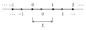
A one-dimensional metamaterial undergoing pure stretching supplies a simple example that illustrates the use of the Fourier transform to compute effective continuum properties. In this case, , , and the joints of the metamaterial define a simple one-dimensional Bravais lattice
| (95) |
where is the length of the members, Fig. 8, and the discrete energy (18) reduces to
| (96) |
with , . Alternatively, the Fourier representation of the discrete deflections is
| (97) |
with , , and the dynamical matrix in (67) reduces to
| (98) |
which, as expected, coincides with the dynamical modulus of a harmonic monatomic chain [49]. The scaled dynamical modulus (70) is
| (99) |
Passing to the continuum limit (82), we obtain
| (100) |
which is the dynamic modulus of a linear elastic bar. The corresponding continuum energy (79) is
| (101) |
or, in real space,
| (102) |
which is the elastic energy of a bar.
4.2. One-dimensional metamaterial with bending
A one-dimensional metamaterial undergoing pure bending illustrates the scaling rule (70). Suppose that the metamaterial has the same geometry and Fourier representation as Example 4.1, Fig. 8, albeit with displacements , where are normal joint deflections and are joint rotations. In this case, the discrete energy (18) reduces to
| (103) |
or to (67), in the Fourier representation, with
| (104) |
The scaled dynamical modulus (70) is
| (105) |
Passing to the continuum limit (82), we obtain
| (106) |
which is the dynamic matrix of a linear elastic beam. The corresponding continuum energy (79) is
| (107) |
or, in real space,
| (108) |
which penalizes departures between the rotation field and the deflection-compatible rotations .
As expected, the bending strains are negligible to zeroth-order and drop out from the energy in the limit. We note that, in this example there is no axial stiffness to stabilize the continuum limit. Under these conditions, to lowest-order any pair of functions and such that define a zero-energy mode and the continuum limit is unstable.
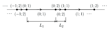
4.3. Two-bar one-dimensional metamaterial
A one-dimensional metamaterial combining two types of bars illustrates the energy relaxation that takes place at the unit cell level in passing to the continuum limit. In this case, , , and the joints of each class define the simple one-dimensional Bravais lattices
| (109a) | ||||
| (109b) | ||||
where and are the lengths of the two classes of members, cf. Fig. 9. Since the members can be classified into two classes of identical members, we additionally have . The discrete energy (18) reduces to
| (110) |
with , , . Alternatively, the Fourier representation of the discrete deflections is
| (111) |
with , , , and the dynamical matrix in (67) reduces to
| (112) |
The scaled dynamical modulus (70) in turn is
| (113) |
Passing to the continuum limit (78), with
| (114) |
gives
| (115) |
where, in the prefactor of , we recognize the effective modulus of two bars connected in series, as expected. With this identification, the continuum energy reduces to the forms (101) and (102).
It bears emphasis that the attainment of the correct limit requires the cell-wise relaxation step encoded in the limit (78). Indeed, we note from (113) that diverges as and, therefore, a naïeve pointwise limit of the energy fails. We also note that, contrariwise, is finite, but the limiting matrix is singular for fixed and cannot be inverted. Only when is projected by , as in (78), is the resulting matrix invertible and a proper limit is defined.
4.4. Two-dimensional honeycomb metamaterial
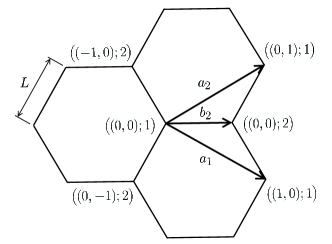
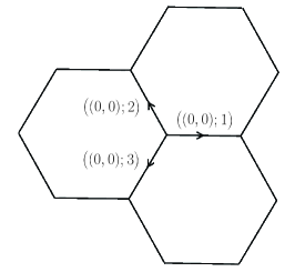
The honeycomb metamaterial of size is two dimensional, , and contains two types of joints, , and three types of oriented bars, , Fig. 10. A possible choice of Bravais lattice and shifts is, Fig. 10a,
| (116a) | ||||
| (116b) | ||||
The volume of the corresponding unit cell is [50]
| (117) |
Fig. 10b shows a choice of indexing for the three types of bars and a choice of bar orientation. The spanning vectors for the three classes of bars are
| (118) |
A direct evaluation of (62), (63) and (64), followed by a computation of the limit (78), gives the limiting continuum energy
| (119) |
in terms of elastic and micropolar components, respectively. In the elastic part of the energy,
| (120) |
are continuum strains and
| (121) |
are effective elastic moduli, explicitly,
| (122) |
We note that the continuum energy is isotropic in the plane, as expected from the hexagonal symmetry of the lattice.
4.5. Three-dimensional octet metamaterial
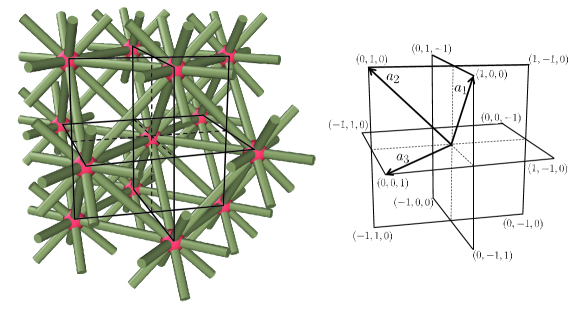
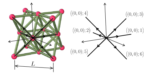
The octet-truss metamaterial of size is three dimensional, , and contains one type of joints, , and six types of oriented bars, , Fig. 11. A possible choice of Bravais lattice is, Fig. 11a,
| (123a) | |||
| (123b) | |||
| (123c) | |||
In addition, Fig. 11b shows an indexing for the three types of bars and a choice of bar orientation. The volume of the corresponding unit cell is [48]
| (124) |
The bar vectors for the six classes of bars are
| (125) |
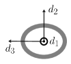
For simplicity, we assume isotropic moments of inertia, , e. g., corresponding to a thin-walled circular cross section. Under this assumption, the choice of directors and is immaterial, provided that they define an orthonormal triad together with . For definiteness, in calculations we choose
| (126) |
where in the Cartesian reference frame.
A direct evaluation of (62), (63) and (64), followed by a computation of the limit (78), gives the limiting continuum energy
| (127) |
in terms of elastic and micropolar components, respectively. In the elastic part of the energy,
| (128) |
are continuum strains and
| (129) |
are effective elastic moduli, explicitly,
| (130) |
We verify that . Hence, the continuum strain-energy density has cubic symmetry, while the micropolar energy density is isotropic, as expected from the cubic symmetry of the lattice. It is also interesting to note that the effective moduli are independent of the torsional stiffness of the bars.
5. Summary and discussion
By an appeal to concepts of calculus of variations, including notions of variational convergence (-convergence in mathematical parlance), we have elucidated the continuum limit of linear metastructures under the assumption of a strict separation of micromechanical (small cell size) and macromechanical (large structure) length scales. The continuum limit of metastructures is of the discrete-to-continuum type [46, 41], but it is non-standard due to presence of bending and rotational degrees of freedom. By an interpolation argument, the continuum limit of metastructures can also be formulated as a homogenization limit [39]. Based on this connection, we argue that the limiting continuum energy is of the integral type, with a well-defined energy density that depends on local gradients and attendant natural boundary conditions. The elucidation of the limiting energy density is greatly facilitated by the assumption of linear elasticity and the corresponding quadratic form of the discrete energy. We have presented a procedure based on the discrete Fourier transform that yields explicitly the effective moduli in the continuum limit, and illustrated the procedure by means of elementary examples and two common metamaterials: a two-dimensional honeycomb lattice and a three-dimensional octet-truss.
The analysis presented in the foregoing sheds light on—and raises—a number of questions, which we briefly discuss next in closing.
The variational continuum limit is unique. The
variational limit of an infinitely fine metastructure of given domain is characterized by the unique continuum energy that matches exactly the limiting minimum potential energies of a sequence of increasingly fine metastructures for all admissible forcings [45]. By extension, it is also the unique continuum energy that matches exactly the limiting values of any macrostructural quantity of interest that depends continuously on the total energy, such as reactions or load-displacement relations. In this sense, the variational continuum limit fulfills its intended aim of being indistinguishable to a macroscopic observer from a sufficiently fine metastructure.
The variational limit also has the unique property of being lossless, in the sense that any displacement solution of the limiting continuum problem is the limit, in a precise sense, of the discrete displacement solutions of the corresponding sequence of increasingly fine metastructures. In particular, the approximating sequence of discrete displacements can be reconstructed, is desired, from the continuum solution at no loss of information.
By virtue of these properties, the variational continuum limit is optimal and superior to any other ad hoc continuum model thereof. In particular, ad hoc continuum models of fine metastructures different from the variational continuum limit are sure to result in gaps between the continuum energy and the limiting energies of the metastructures, and, by extension, also in gaps in any other macroscopic quantity of interest, at least for some forcings.
The continuum limit is micropolar and local. By a rigorous computation of the variational continuum limit of infinitely fine metastructures, we have shown that the limiting continuum energy is micropolar, in the sense of [42]. However, to lowest order the continuum energy is independent of the curvature of the deformation, or bending strain, and therefore local. In particular, the lowest-order continuum limit exhibits linear-elastic volume scaling and fails to capture size effects such as observed in fracture experiments at the mesoscale [26]. The scope of the lowest-order continuum limit is therefore limited to applications in which size effects can be neglected, such as the analysis of lightweight structures under normal operating conditions, cf., e. g., [51, 52] for representative applications to aerospace structures.
Higher-order expansions and size effects. Evidently, the local character of the continuum limit to lowest order owes to the assumption of strict scale separation. In situations where non-local or mesoscale effects are important, the lowest-order limit needs to be augmented with fine-scale information. The full micropolar model of the honeycomb metastructure proposed by [25] is an early example in that regard. As mentioned in the introduction, computational schemes have been proposed that coarse-grain the description of a metastructure while retaining full resolution where required [31, 30].
Alternatively, higher-order generalized continuum models can be systematically formulated by recourse to the method of variational -equivalence [53]. We recall that a sequence of energy functionals is variationally equivalent to another to order as if
| (131) |
for all admissible forcings , where , respectively , is the minimum potential attained by , respectively , under forcing . The fundamental property of variational equivalence (see [53, Theorems 4.3 and 4.4] is that, provided that and are stable in the sense of equicoercivity, their low-energy configurations converge to the same limit. In addition, any macroscopic quantity of interest computed from is indistinguishable from the same quantity computed from to order .
The variational -equivalence framework thus provides a rigorous means of defining sequences of mesoscopic continuum models that have the same continuum limit as the sequence of discrete metastructural energies and, in addition, exhibit the same asymptotic behavior to order . For instance, for it is readily verified that a formal Taylor series expansion of to order in , namely,
| (132) |
generates a sequence of continuum energies that is variationally equivalent to the discrete metastructural energies to order . It should be carefully noted that variationally equivalent energies of the same order are not unique, and particular choices thereof are, to a certain extent, a matter of convenience or expediency. However, variational equivalence does provide a rigorous criterion to weed out non-equivalent and, therefore, non-performing models.
In the present context, the higher-order extensions of the continuum limit, such as the full micropolar model proposed by [25] for honeycomb metastructures, are non-local and therefore exhibit a size effect. By assuming the bars to have a finite strength, they also endow the limiting continuum with a well-defined fracture toughness [25]. It remains to verify whether these enhancements of the theory suffice to capture observed size effects, such as the specimen-size dependence of fracture toughness [26].
Acknowledgements
S. Conti and M. Ortiz gratefully acknowledge the support of the Deutsche Forschungsgemeinschaft (DFG, German Research Foundation) via project 211504053 - SFB 1060; project 441211072 - SPP 2256; and project 390685813 - GZ 2047/1 - HCM. P. Ariza gratefully acknowledges financial support from Ministerio de Ciencia e Innovación under grant number PID2021-124869NB-I00.
Appendix A The discrete Fourier transform
Let be a basis of and the corresponding Bravais lattice. Let be a real-valued lattice function. The discrete Fourier transform of is a complex function supported on the Brillouin zone in dual space given by
| (133) |
where is the volume of the unit cell of the lattice. The inverse mapping is given by
| (134) |
The convolution of two lattice functions , is
| (135) |
whereupon the convolution theorem states that
| (136) |
In addition, the Parseval identity states that
| (137) |
which establishes an isometric isomorphism between and (cf. [48] and references therein for further details).
Appendix B Structure of continuum energy
Let . From (70), we have
| (138) |
Rescale as
| (139) |
Then, from (138),
| (140) |
where we have used (70) again. By duality,
| (141) |
Writing
| (142) |
we have the decomposition
| (143) |
in terms of deflections and rotations. Inserting into (141) we obtain, explicitly,
| (144) |
Passing to the limit using (78) further gives
| (145) |
with
| (146) |
Finally, by duality we have
| (147) |
Decomposing as in (84), to match (146), the duality pairing has the decomposition
| (148) |
and (147) evaluates to
| (149) |
or equivalently (83), as surmised.
References
- [1] L. Montemayor, V. Chernow, and J.R. Greer. Materials by design: Using architecture in material design to reach new property spaces. MRS Bulletin, 40(12):1122–1129, 2015.
- [2] Julia R. Greer and Vikram S. Deshpande. Three-dimensional architected materials and structures: Design, fabrication, and mechanical behavior. MRS Bulletin, 44(10):750–757, 2019.
- [3] C. Lu, M. Hsieh, Z. Huang, C. Zhang, Y.Lin, Q.Shen, F. Chen, and L. Zhang. Architectural design and additive manufacturing of mechanical metamaterials: A review. Engineering, 17:44–63, 2022.
- [4] N.A. Fleck, V.S. Deshpande, and M.F. Ashby. Micro-architectured materials: Past, present and future. Proceedings of the Royal Society A: Mathematical, Physical and Engineering Sciences, 466(2121):2495–2516, 2010.
- [5] M. Benedetti, A. du Plessis, R.O. Ritchie, M. Dallago, N. Razavi, and F. Berto. Architected cellular materials: A review on their mechanical properties towards fatigue-tolerant design and fabrication. Materials Science and Engineering: R: Reports, 144:100606, 2021.
- [6] L. Wu, Y. Wang, K. Chuang, F. Wu, Q. Wang, W. Lin, and H. Jiang. A brief review of dynamic mechanical metamaterials for mechanical energy manipulation. Materials Today, 44:168–193, 2021.
- [7] X. Xia, C.M. Spadaccini, and J.R. Greer. Responsive materials architected in space and time. Nature Reviews Materials, 7(9):683–701, 2022.
- [8] H. Jin and H.D. Espinosa. Mechanical metamaterials fabricated from self-assembly: A perspective. Journal of Applied Mechanics, Transactions ASME, 91(4), 2024.
- [9] R. Hamzehei, M. Bodaghi, and N. Wu. 3d-printed highly stretchable curvy sandwich metamaterials with superior fracture resistance and energy absorption. International Journal of Solids and Structures, 286-287:112570, 2024.
- [10] M.F. Ashby. The properties of foams and lattices. Philosophical Transactions of the Royal Society A: Mathematical, Physical and Engineering Sciences, 364(1838):15–30, 2006.
- [11] J.-H. Lee, L. Wang, M.C. Boyce, and E.L. Thomas. Periodic bicontinuous composites for high specific energy absorption. Nano Lett, 12:4392–4396, 2012.
- [12] D. Jang, L.R. Meza, F. Greer, and J.R. Greer. Fabrication and deformation of three-dimensional hollow ceramic nanostructures. Nature Mater, 12:893–898, 2013.
- [13] J. Bauer, S. Hengsbach, I. Tesari, R. Schwaiger, and O. Kraft. High-strength cellular ceramic composites with 3D microarchitecture. Proc. Natl. Acad. Sci. USA, 111:2453–2458, 2014.
- [14] L.R. Meza, S. Das, and J.R. Greer. Strong, lightweight, and recoverable threedimensional ceramic nanolattices. Science, 345:1322–1326, 2014.
- [15] J. Rys, L. Valdevit, T.A. Schaedler, A.J. Jacobsen, W.B. Carter, and J.R. Greer. Fabrication and deformation of metallic glass micro-lattices. Adv. Eng. Mater, 16:889–896, 2014.
- [16] X. Zheng, H. Lee, T.H. Weisgraber, M. Shusteff, J. DeOtte, E.B. Duoss, J.D. Kuntz, M.M. Biener, Q. Ge, J.A. Jackson, S.O. Kucheyev, N.X. Fang, and C.M. Spadaccini. Ultralight, ultrastiff mechanical metamaterials. Science, 344:1373–1377, 2014.
- [17] L.R. Meza, A.J. Zelhofer, N. Clarke, A.J. Mateos, D.M. Kochmann, and J.R. Greer. Resilient 3d hierarchical architected metamaterials. Proc. Natl. Acad. Sci. USA, 112:11502–11507, 2015.
- [18] X.Wendy Gu and J.R. Greer. Ultra-strong architected Cu meso-lattices. Extreme Mech. Lett, 2:7–14, 2015.
- [19] J. Bauer, A. Schroer, R. Schwaiger, I. Tesari, C. Lange, L. Valdevit, and O. Kraft. Push-to-pull tensile testing of ultra-strong nanoscale ceramic–polymer composites made by additive manufacturing. Extreme Mech. Lett, 3:105–112, 2015.
- [20] J. Bauer, A. Schroer, R. Schwaiger, and O. Kraft. Approaching theoretical strength in glassy carbon nanolattices. Nature Mater, 15:438–443, 2016.
- [21] V. Deshpande, N. Fleck, and M. Ashby. Effective properties of the octet-truss lattice material. J. Mech. Phys. Solids, 49:1747–1769, 2001.
- [22] J.J. Rosário, E.T. Lilleodden, M. Waleczek, R. Kubrin, AYu Petrov, P.N. Dyachenko, J.E.C. Sabisch, K. Nielsch, N. Huber, M. Eich, and G.A. Schneider. Selfassembled ultra high strength, ultra stiff mechanical metamaterials based on inverse opals. Adv. Eng. Mater, 17:1420–1424, 2015.
- [23] J.J. do Rosário, J.B. Berger, E.T. Lilleodden, R.M. McMeeking, and G.A. Schneider. The stiffness and strength of metamaterials based on the inverse opal architecture. Extreme Mechanics Letters, 12:86–96, 2017.
- [24] V. Deshpande, M. Ashby, and N. Fleck. Foam topology: bending versus stretching dominated architectures. Acta Mater, 49:1035–1040, 2001.
- [25] J.Y. Chen, Y. Huang, and M. Ortiz. Fracture analysis of cellular materials: A strain gradient model. Journal of the Mechanics and Physics of Solids, 46(5):789–828, 1998.
- [26] A.J.D. Shaikeea, H. Cui, M. O’Masta, X.R. Zheng, and V.S. Deshpande. The toughness of mechanical metamaterials. Nature Materials, 21(3):297–304, 2022.
- [27] M. Maurizi, B.W. Edwards, C. Gao, J.R. Greer, and F. Berto. Fracture resistance of 3d nano-architected lattice materials. Extreme Mechanics Letters, 56, 2022.
- [28] S. Luan, E. Chen, and S. Gaitanaros. Energy-based fracture mechanics of brittle lattice materials. Journal of the Mechanics and Physics of Solids, 169, 2022.
- [29] P. Zhang, P. Yu, R. Zhang, X. Chen, and H. Tan. Grid octet truss lattice materials for energy absorption. International Journal of Mechanical Sciences, 259:108616, 2023.
- [30] G.P. Phlipot and D.M. Kochmann. A quasicontinuum theory for the nonlinear mechanical response of general periodic truss lattices. Journal of the Mechanics and Physics of Solids, 124:758–780, 2019.
- [31] Dennis M Kochmann, Jonathan B Hopkins, and Lorenzo Valdevit. Multiscale modeling and optimization of the mechanics of hierarchical metamaterials. MRS Bulletin, 44(10):773–781, 2019.
- [32] E. B. Tadmor, M. Ortiz, and R. Phillips. Quasicontinuum analysis of defects in solids. Philosophical Magazine a-Physics of Condensed Matter Structure Defects and Mechanical Properties, 73(6):1529–1563, 1996.
- [33] E. B. Tadmor, R. Phillips, and M. Ortiz. Mixed atomistic and continuum models of deformation in solids. Langmuir, 12(19):4529–4534, 1996.
- [34] M. I. Español, D. M. Kochmann, S. Conti, and M. Ortiz. A -convergence analysis of the quasicontinuum method. SIAM Multiscale Modeling & Simulation, 11(3):766–794, 2013.
- [35] Tim Fabian Korzeniowski and Kerstin Weinberg. Data-driven finite element computation of open-cell foam structures. Computer Methods in Applied Mechanics and Engineering, 400:115487, 2022.
- [36] Kerstin Weinberg. Data-driven finite element computation of microstructured materials. PAMM, 23(4):e202300285, 2023.
- [37] P. Jiao, J. Mueller, J.R. Raney, X. Zheng, and A.H. Alavi. Mechanical metamaterials and beyond. Nature Communications, 14(6004), 2023.
- [38] K. Karapiperis and D.M. Kochmann. Prediction and control of fracture paths in disordered architected materials using graph neural networks. Communications Engineering, 2:32, 2023.
- [39] D. Cioranescu and P. Donato. An introduction to homogenization, volume 17 of Oxford Lecture Series in Mathematics and its Applications. The Clarendon Press Oxford University Press, New York, 1999.
- [40] M. Cicalese, A. DeSimone, and C. I. Zeppieri. Discrete-to-continuum limits for strain-alignment-coupled systems: Magnetostrictive solids, ferroelectric crystals and nematic elastomers. Networks and Heterogeneous Media, 4(4):667–708, 2009.
- [41] Andrea Braides and Maria Stella Gelli. From discrete systems to continuous variational problems: an introduction. In Topics on concentration phenomena and problems with multiple scales, volume 2 of Lect. Notes Unione Mat. Ital., pages 3–77. Springer, Berlin, 2006.
- [42] A.C. Eringen. Linear theory of micropolar elasticity. Journal of Mathematics and Mechanics, 15(6):909–923, 1966.
- [43] H. Askes and E.C. Aifantis. Gradient elasticity in statics and dynamics: An overview of formulations, length scale identification procedures, finite element implementations and new results. International Journal of Solids and Structures, 48:1962–1990, 2011.
- [44] S. P. Timoshenko and D. H. Young. Theory of Structures. McGraw-Hill Book Company, New York, 2nd edition, 1965.
- [45] G. dal Maso. An introduction to -convergence. Progress in Nonlinear Differential Equations and their Applications, 8. Birkhäuser Boston Inc., Boston, MA, 1993.
- [46] R. Alicandro and M. Cicalese. A general integral representation result for continuum limits of discrete energies with superlinear growth. SIAM Journal on Mathematical Analysis, 36(1):1–37, 2004.
- [47] S. Mallat. A wavelet tour of signal processing. Elsevier/Academic Press, Amsterdam, third edition, 2009. The sparse way, With contributions from Gabriel Peyré.
- [48] M.P. Ariza and M. Ortiz. Discrete crystal elasticity and discrete dislocations in crystals. Archive for Rational Mechanics and Analysis, 178(2):149–226, 2005.
- [49] J. H. Weiner. Statistical mechanics of elasticity. Dover Publications, Mineola, N.Y., 2nd edition, 2002.
- [50] M. P. Ariza and M. Ortiz. Discrete dislocations in graphene. Journal of the Mechanics and Physics of Solids, 58(5):710–734, 2010.
- [51] Kenneth C. Cheung and Neil Gershenfeld. Reversibly assembled cellular composite materials. Science, 341(6151):1219–1221, 2013.
- [52] Christine E. Gregg, Damiana Catanoso, Olivia Irene B. Formoso, Irina Kostitsyna, Megan E. Ochalek, Taiwo J. Olatunde, In Won Park, Frank M. Sebastianelli, Elizabeth M. Taylor, Greenfield T. Trinh, and Kenneth C. Cheung. Ultralight, strong, and self-reprogrammable mechanical metamaterials. Science Robotics, 9(86):eadi2746, 2024.
- [53] A. Braides and L. Truskinovsky. Asymptotic expansions by -convergence. Continuum Mechanics and Thermodynamics, 20:21–62, 2008.