The Blind Normalized Stein Variational Gradient Descent-Based Detection for Intelligent Massive Random Access

Abstract

The lack of an efficient preamble detection algorithm remains a challenge for solving preamble collision problems in intelligent massive random access (RA) in practical communication scenarios. To solve this problem, we present a novel early preamble detection scheme based on a maximum likelihood estimation (MLE) model at the first step of the grant-based RA procedure. A novel blind normalized Stein variational gradient descent (SVGD)-based detector is proposed to obtain an approximate solution to the MLE model. First, by exploring the relationship between the Hadamard transform and wavelet transform, a new modified Hadamard transform (MHT) is developed to separate high-frequencies from important components using the second-order derivative filter. Next, to eliminate noise and mitigate the vanishing gradients problem in the SVGD-based detectors, the block MHT layer is designed based on the MHT, scaling layer, soft-thresholding layer, inverse MHT and sparsity penalty. Then, the blind normalized SVGD algorithm is derived to perform preamble detection without prior knowledge of noise power and the number of active devices. The experimental results show the proposed block MHT layer outperforms other transform-based methods in terms of computation costs and denoising performance. Furthermore, with the assistance of the block MHT layer, the proposed blind normalized SVGD algorithm achieves a higher preamble detection accuracy and throughput than other state-of-the-art detection methods.

I Introduction

Given the prevalence of massive machine-type communication (mMTC) [1, 2], the forthcoming wireless communication system is required to accommodate the extensive network of devices. However, there can be challenges related to the potential preamble collision [3, 4, 5] issues, particularly when a considerable number of devices attempt to access the network simultaneously. Furthermore, effectively detecting or tackling preamble collision is crucial for the implementation of Internet of Things (IoT) scenarios [6]. Currently, to reduce transmission latency and signaling overhead, a range of strategies, such as grant-based and grant-free random access (RA) schemes, are utilized to mitigate preamble collision problems in mMTC.

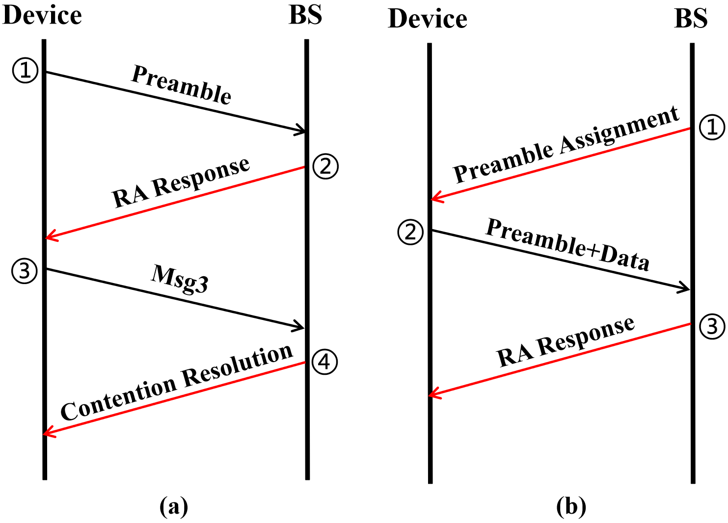
Figure 1: (a) The grant-based RA procedure. (b) The grant-free RA procedure.

The currently standardized procedure for device access in IoT networks is grant-based RA [7, 8, 9, 10, 11]. It utilizes a communication protocol where devices seek and obtain permission prior to transmitting data on the network. As shown in Fig. 1, in the first stage, every active device randomly chooses a preamble from the pool at each time slot. After that, the base station (BS) transmits the RA responses corresponding to the activated preambles. Next, active devices send message 3 (MSG3), requesting the BS to allocate resources for data transmission. Finally, if the preamble sent in Step 1 is chosen by a single user, the BS will grant the corresponding request and send a contention-resolution message to inform the active device of the available resources. Otherwise, a preamble collision happens. The conflicting devices will not be granted permission and will retry access in the next time slot.

Unlike grant-based RA, each active device directly transmits the preamble and data to the BS without any permission under the grant-free RA schemes [12, 13, 14]. Additionally, each user is pre-assigned a dedicated preamble, which can also serve as the user ID. In each time slot, the BS first detects preambles to identify active devices. Subsequently, the BS performs channel estimation based on metadata and decodes data using the acquired channel information. Compared with grant-based RA, grant-free RA alleviates preamble collisions and reduces access latency. However, assigning orthogonal preambles to massive devices is not feasible. Therefore, it is a challenging task to detect active devices under grant-free RA [15]. Additionally, grant-free RA often leads to unreliable transmissions [16]. Hence, to ensure high-rate transmissions alongside both extensive access and reliable connectivity, we consider the grant-based RA scheme in this paper.

I-A Early preamble collision detection schemes

In the grant-based RA scheme, the preamble collision can only be identified in the fourth step. Therefore, in the second step, the BS still allocates wireless resources to devices involved in collisions. It results in a waste of wireless resources. To address this issue, the authors of [17] introduced an early preamble collision detection (e-PACD) scheme based on the tagged preambles at the first step of grant-based RA. The tagged preambles consist of the preambles and tag Zadoff-Chu (ZC) sequences with different root numbers. The e-PACD scheme determines preamble collision by detecting whether the same preamble contains multiple tags. However, the overuse of root sequences escalates the complexity of detection. Besides, as ZC sequences with varying root indexes lack orthogonality, the frequency of false alarms rises alongside the number of root sequences utilized in correlation operations. Additionally, a single-root preamble sequence-based early collision detection scheme was proposed for satellite-based IoT [18] at the first step of grant-based RA. In the scheme, all feasible preambles are generated using the ZC sequence with different cyclic shifts. The intricate design of the cyclic shift offset set improves the efficiency of preamble collision detection at the second step. However, the cyclic shift offsets increase the complexity of the preamble design. Moreover, since the single root ZC sequences are employed, the number of preambles is limited, leading to increasing the probability of preamble collision in a dense user scenario.

I-B Preamble Detection Algorithms

The appropriate preamble detection algorithms are crucial for detecting preamble collisions in advance. In [19], a maximum a posteriori (MAP) estimation model was proposed for detecting preambles. A low-complexity Markov Chain Monte Carlo (MCMC) algorithm was employed to sample the MAP model to obtain an approximate solution. However, the MCMC algorithm increases estimation errors due to the stochastic nature of sampling. To enhance the accuracy of the MCMC-based scheme, the normalized Stein Variational Gradient Descent (NSVGD) detector [20] was proposed based on the maximum likelihood estimation (MLE) model. The NSVGD detector enhances the accuracy of preamble detection through the deterministic update characteristics of particles. However, to improve robustness in low signal-to-noise ratio (SNR) environments, the NSVGD detector introduces a bias term. This bias term necessitates the BS to know the number of active devices. In practical communication scenarios, it is challenging to obtain the number of active devices in the cell. Moreover, the authors of [21] established a maximum likelihood preamble detection model based on non-Bayesian methods. The non-Bayesian method offers lower computational complexity, enabling rapid preamble detection. Nevertheless, the non-Bayesian approach cannot be used to detect preamble collisions. Furthermore, deep learning methods have been applied for solving detection problems. In [22], the convolutional neural network-based approach was employed to detect preambles by extracting features from signals.

I-C Motivations and Contributions

The early preamble collision detection schemes make it possible to improve the efficiency of wireless resource utilization [23]. Therefore, this paper develops a novel preamble detection scheme at the first step of the grant-based RA process. Instead of designing the complicated preambles to detect preamble collision [15, 18], we utilize the non-orthogonal Gaussian preambles with a simple structure, which is suitable for a dense user scenario. Additionally, we design an efficient maximum likelihood preamble detection model using the blind NSVGD-based detector, which strives to fully exploit the potential of the NSVGD detector to improve the preamble detection accuracy. More specifically, first, by investigating the connection between the Hadamard transform and Haar wavelet transform, we design a new modified Hadamard transform (MHT) by replacing the last half rows in the Hadamard matrix with the second-order derivative filter. Based on the MHT, a new block MHT domain layer is proposed. We developed the discrete cosine transform (DCT) and Hadamard transform domain layers in several applications [24, 25, 26, 27]. In this paper, the key idea is to apply the MHT, scaling layer, trainable soft-thresholding layer, and Kullback Leibler divergence-based sparsity penalty to remove the noise from the complex signals. Then, we derive a new blind NSVGD algorithm that combines the SVGD algorithm and momentum strategy to perform preamble detection. The main contributions are concluded as follows:

1. A novel MHT is designed by modifying the Hadamard matrix. Compared with the Hadamard transform, the MHT has a better ability to separate high-frequency bands from important components in the transform domain.

2. An efficient block MHT layer is proposed to denoise the signal received by the BS, which helps to alleviate the vanishing gradient problem and enhance the robustness of the NSVGD detector in noisy environments. Compared with other state-of-the-art methods, the block MHT layer achieves a better denoising performance with a lower computation cost.

3. A new blind NSVGD algorithm is derived. In comparison to the NSVGD detector, the blind NSVGD algorithm is capable of finishing preamble detection without the knowledge of noise power and the number of active devices, making it feasible for implementation in practical communication scenarios.

4. The experimental results show that the proposed preamble detection scheme achieves a higher preamble detection accuracy and better robustness than other baselines under different SNRs and different numbers of antennas and active devices. Additionally, the proposed method is superior to other schemes in terms of throughput.

The remainder of the paper is structured as follows. Section II describes the maximum likelihood preamble detection model at the first step of grant-based RA. The introduction and error analysis of SVGD-based detectors are provided in Section III. The blind NSVGD-based detector is derived in Section IV. Simulation results are presented in Section V. Finally, conclusions are given in Section VI.

II System Model

Suppose the BS is equipped with $T$ antennas, and each active device in the cell is equipped with one antenna. Each preamble is randomly chosen by each active device from the pool. The length of each preamble is $L$. Additionally, assume the signals transmitted by the active devices experience Rayleigh fading. Then, the signal received by the BS on the $t$-th antenna can be computed as follows:

$$\mathbf{y}_{t}=\sum_{m=1}^{M}\mathbf{z}_{(m)}H_{m,t}e_{m}+\mathbf{n}_{t},$$ (1)

for $t=1,\dots,T$, where $M$ stands for the number of active devices. $\mathbf{z}_{(m)}\sim\mathcal{CN}(0,1/L)$ is the non-orthogonal preamble chosen by the $m$-th active device. $\mathcal{CN}(\mathbf{a},\mathbf{B})$ stands for the circularly symmetric complex Gaussian (CSCG) distribution, which has a mean vector $\mathbf{a}$ and a covariance matrix $\mathbf{B}$. Additionally, $\mathbf{n}_{t}\sim\mathcal{CN}(0,\delta\mathbf{I})$ represents the background noise and $\delta$ represents the noise power. $H_{m,t}$ indicates the channel coefficient. $e_{m}$ denotes the data symbol transmitted from the active device to the BS.

Assume the number of preambles is $K$ and $x_{k}\in[0,M]$ denotes the number of active devices choosing the $k$-th preamble. The vector $\mathbf{x}=[x_{1},\dots,x_{k},\dots,x_{K}]^{\mathrm{T}}$ stands for the numbers of active devices choosing each preamble. As our target is to detect preamble collisions in the first step of grant-based RA, we concentrate on estimating $\mathbf{x}$ in the subsequent steps: First of all, the likelihood of $\mathbf{x}$ is computed as follows:

$${\rm{Lik}(\mathbf{x})}=f({\mathbf{y}_{t}}\mid\mathbf{x}),$$ (2)

After that, let $\mathbf{v}_{t}=[v_{1,t},v_{2,t},\dots,v_{k,t},\dots,v_{K,t}]^{\mathrm{T}}$, and

$$v_{k,t}=\sum_{m\in\mathcal{\mathcal{N}}_{k}}H_{m,t}e_{m},$$ (3)

where $\mathcal{N}_{k}$ represents the index set of active devices choosing the $k$-th preamble. Suppose $H_{m,t}\sim\mathcal{CN}(0,\beta^{2})$, we have:

$$\begin{array}[]{l}f(\mathbf{v}_{t}|\mathbf{x})=\prod\limits_{k\in\mathcal{\zeta^{+}(\mathbf{x})}}\frac{1}{\pi\beta^{2}x_{k}}\exp(-\frac{{\lvert v_{k,t}\rvert}^{2}}{\beta^{2}x_{k}}),\end{array}$$ (5)

where $\mathcal{\zeta^{+}(\mathbf{x})}=\{k\mid x_{k}\textgreater 0\}$. Next, let $\mathbf{Z}=[\mathbf{z}_{1},\dots,\mathbf{z}_{K}]$. $\mathbf{y}_{t}$ in the Eq. (1) can be caculated as follows:

$$\mathbf{y}_{t}=\mathbf{Z}\mathbf{v}_{t}+\mathbf{n}_{t},$$ (6)

According to $\mathbf{n}_{t}\sim\mathcal{CN}(0,\delta\mathbf{I})$, we have:

$$\begin{array}[]{l}f(\mathbf{y}_{t}|\mathbf{v}_{t})=\frac{1}{(\pi\delta)^{L}}\exp(-\frac{1}{\delta}\|\mathbf{y}_{t}-\mathbf{Z}\mathbf{v}_{t}\|^{2}).\end{array}$$ (8)

From Eq. (5), Eq. (6) and Eq. (8), the mean value of $\mathbf{y}_{t}$ is zero and its covariance matrix is computed as follows:

$$\mathbb{E}[\mathbf{y}_{t}\mathbf{y}_{t}^{\mathrm{H}}\mid\mathbf{x}]=\beta^{2}\mathbf{Z}\mathbf{C}_{\mathbf{x}}\mathbf{Z}^{\mathrm{H}}+\delta\mathbf{I}=\varphi(\mathbf{x}),$$ (9)

where $\mathbf{C}_{\mathbf{x}}$ = diag$(x_{1}\dots x_{K})$. $(\cdot)^{\mathrm{H}}$ represents the conjugate transpose. From Eq. (9), $\mathbf{y}_{t}$ is a CSCG vector:

$$\mathbf{y}_{t}\mid\mathbf{x}\sim\mathcal{CN}(\mathbf{0},\varphi(\mathbf{x})),$$ (10)

$$\begin{array}[]{l}f(\mathbf{y}_{t}\mid\mathbf{x})=\frac{1}{(\pi^{L})\det(\varphi(\mathbf{x}))}e^{-\mathbf{y}_{t}^{\mathrm{H}}\varphi(\mathbf{x})^{-1}\mathbf{y}_{t}}.\end{array}$$ (12)

Then $\{\mathbf{y}_{t}\}_{t=1}^{T}$ is defined as the set of received signals across $T$ antennas. Its likelihood function is:

$$f(\{\mathbf{y}_{t}\}_{t=1}^{T}\mid\mathbf{x})=\prod\nolimits_{t=1}^{T}f(\mathbf{y}_{t}\mid\mathbf{x}),$$ (13)

Furthermore, its log-likelihood function is:

$$\begin{aligned} \ln f(\{\mathbf{y}_{t}\}_{t=1}^{T}\mid\mathbf{x})&=\sum\limits_{t=1}^{T}\ln f(\mathbf{y}_{t}\mid\mathbf{x})\\ &=\sum\limits_{t=1}^{T}-\mathbf{y}_{t}^{\mathrm{H}}\varphi(\mathbf{x})^{-1}\mathbf{y}_{t}-\ln\det(\varphi(\mathbf{x}))+\eta,\end{aligned}$$ (14)

where $\eta$ is a constant. Finally, the maximum log-likelihood estimation model can be obtained by utilizing the log-likelihood function:

$$\tilde{\mathbf{x}}=\mathop{\arg\max}\ln f(\{\mathbf{y}_{t}\}_{t=1}^{T}\mid\mathbf{x}).$$ (15)

The computational complexity of maximum likelihood estimation is $(M+1)^{K}$, which grows exponentially with $K$. Hence, as $K$ increases, the computational complexity escalates significantly.

III svgd based preamble detection

Due to the high computational complexity associated with directly solving the maximum likelihood detection model, some variational inference methods are applied to obtain an approximate solution, e.g., SVGD-based algorithms. Therefore, we introduce the SVGD-based approaches for the preamble detection problem in this section.

III-A Stein Variational Gradient Descent (SVGD)

SVGD [28, 29, 30, 31] is a particle-based variational inference algorithm used for gradient descent optimization. The algorithm iteratively updates particles to gradually transition from the initial distribution to the target distribution by minimizing the KL divergence between the two distributions. A set of particles are first initialized with an arbitrary distribution. Next, the particles are updated using the optimal perturbation direction, which corresponds to the steepest descent on the KL divergence. After multiple iterations, the particles converge towards the target distribution. By leveraging the gradient information of the target distribution, SVGD offers a flexible and scalable approach to take samples from the complicated distribution.

III-B SVGD Detector

To solve the preamble detection problem, we employed the SVGD algorithm to obtain an approximate solution to the maximum likelihood model [20]. The key idea is applying SVGD to sample $\mathbf{x}$ from the target distribution $p(\mathbf{x})$. Here, the density function of $p(\mathbf{x})$ is $g(\mathbf{x})=f(\{\mathbf{y}_{t}\}\mid\mathbf{x})$. It is mentioned in [28] that the particles can be initialized with any distribution. Therefore, we first use the uniform distribution to initialize a set of particles $\{\mathbf{x}_{u}\}_{u=1}^{n}$. $n$ is the number of particles. Then, for $r$-th iteration, the particles are updated as follows:

$$\mathbf{x}_{u}^{r+1}\leftarrow\mathbf{x}_{u}^{r}+\lambda{\omega}(\mathbf{x}_{u}^{r}),$$ (16)

where $\lambda$ is a step size. $\omega(\cdot)$ is a velocity field, which transports the particles to approximate the target distribution. It is defined as:

$${\omega}(\mathbf{x})=\frac{1}{n}\sum_{i=1}^{n}[k(\mathbf{x}_{i}^{r},\mathbf{x})\bigtriangledown_{\mathbf{x}_{i}^{r}}\ln g(\mathbf{x}_{i}^{r})+\bigtriangledown_{\mathbf{x}_{i}^{r}}k(\mathbf{x}_{i}^{r},\mathbf{x})],$$ (17)

where $k(\mathbf{x}_{i}^{r},\mathbf{x})=\exp(-\frac{1}{h}||\mathbf{x}_{i}^{r}-\mathbf{x}||_{2}^{2})$ is the Gaussian radial basis function (RBF) kernel function [32]. $h={\rm{med}}^{2}/\ln n$. ${\rm{med}}$ is the median of pairwise distances between $\{x_{u}\}_{u=1}^{n}$. After sufficient iterations, the particles $\{\mathbf{\tilde{x}}_{u}\}_{u=1}^{n}$ sampled by SVGD approximate the target distribution $p(\mathbf{x})$. Next, $\{\mathbf{\tilde{x}}_{u}\}_{u=1}^{n}$ is utilized to estimate the number of devices choosing each preamble.

III-C NSVGD Detector

From Eq. (14), it is observed that the value of the MLE function is mainly determined by $\varphi(\mathbf{x})=\beta^{2}\mathbf{Z}\mathbf{C}_{\mathbf{x}}\mathbf{Z}^{\mathrm{H}}+\delta\mathbf{I}$. $\delta$ represents noise power. When the modulus of each entry $\tau$ in matrix $\phi(\mathbf{x})=\beta^{2}\mathbf{Z}\mathbf{C}_{\mathbf{x}}\mathbf{Z}^{\mathrm{H}}$ is much smaller than $\delta$, we have $\varphi(\mathbf{x})\thickapprox\delta\mathbf{I}$, which indicates $\varphi(\mathbf{x})$ is independent to the change of $\phi(\mathbf{x})$. Furthermore, Eq. (14) is rewritten as:

$$\ln g(\mathbf{x}_{u}^{r})=-\sum_{t=1}^{T}\mathbf{y}_{t}^{\mathrm{H}}\mathbf{(}\delta\mathbf{I})^{-1}\mathbf{y}_{t}-T\ln\det(\delta\mathbf{I})+\eta,$$ (18)

Hence, $\bigtriangledown_{\mathbf{x}_{u}^{r}}\ln g(\mathbf{x}_{u}^{r})=0$. Then ${\omega}(\mathbf{x})$ is caculated as:

$${\omega}(\mathbf{x})=\frac{1}{n}\sum_{i=1}^{n}[\bigtriangledown_{\mathbf{x}_{u}^{r}}k(\mathbf{x}_{u}^{r},\mathbf{x})],$$ (19)

According to Eq. (19), it is noticed that only $\bigtriangledown_{\mathbf{x}_{u}^{r}}k(\mathbf{x}_{u}^{r},\mathbf{x})$ is applied to update $\mathbf{x}$. However, $\bigtriangledown_{\mathbf{x}_{u}^{r}}k(\mathbf{x}_{u}^{r},\mathbf{x})$ does not contain any effective information about the target distribution. Then, the particles are updated towards the wrong direction. Therefore, the noise can cause the vanishing gradients problem in the SVGD detector, which increases the estimation errors. To enhance the robustness of the SVGD-based model, we further proposed NSVGD based on the momentum and a bias correction term $\vartheta$, which is defined as:

$$\vartheta=\nu\left(nM-\sum_{u=1}^{n}||\mathbf{x}_{u}^{r}||_{1}\right),$$ (20)

where $\nu$ is constant weight. $\vartheta$ utilizes the number of active devices in the cell as a constraint to correct the direction of particle updates. However, the number of active devices is unknown in practical communication scenarios. Therefore, the NSVGD detector cannot directly be applied in the random access scheme.

IV The blind NSVGD-based detector for preamble detection

As described above, the performance of the SVGD detector is susceptible to environmental noise. Additionally, the NSVGD detector requires unknown prior knowledge to detect the preamble. To address these issues, we propose a novel blind NSVGD-based detector. Firstly, the new modified Hadamard transform (MHT) is introduced to replace the Hadamard transform. Next, the block MHT layer is developed to eliminate noise using the MHT, scaling layer, trainable soft-thresholding layer and inverse MHT. Then, a new blind NSVGD algorithm is designed for preamble detection without requiring unknown prior knowledge.

IV-A The modified Hadamard transform (MHT)

Transform-based denoising methods have become prevalent in data analysis for efficiently reducing noise from signals. These techniques apply mathematical transforms to represent signals in alternate domains, enabling the separation of noise from the underlying structure. Commonly used transforms include the Fourier transform, wavelet transform, Hadamard transform, and discrete cosine transform (DCT). Among them, the Hadamard transform concentrates the majority of the signal energy in a small subset of coefficients. The rest of the coefficients are redundant data. Such energy concentration property allows for separating important components from noise in the transform domain, thus enhancing denoising effectiveness. Given an input vector $\mathbf{x}=[x_{0},x_{1},\dots,x_{D-1}]$, its Hadamard transform $\mathbf{X}=[X_{0},X_{1},\dots,X_{D-1}]$ is defined as:

$$\mathbf{X}=\mathcal{T}(\mathbf{x})=\sqrt{\frac{1}{D}}\mathbf{H}_{D}\mathbf{x},$$ (21)

where the Hadamard matrix $\mathbf{H}_{D}$ is computed as follows:

$$\mathbf{H}_{D}=\begin{cases}1,&D=1,\\ \begin{pmatrix}[r]1&1\\ 1&-1\end{pmatrix},&D=2,\\ \begin{pmatrix}[r]\mathbf{H}_{\frac{D}{2}}&\mathbf{H}_{\frac{D}{2}}\\ \mathbf{H}_{\frac{D}{2}}&-\mathbf{H}_{\frac{D}{2}}\end{pmatrix},&D\geq 4,\end{cases}$$ (22)

The inverse Hadamard transform is defined as:

$$\mathbf{x}=\mathcal{T}^{-1}(\mathbf{X})=\sqrt{\frac{1}{D}}\mathbf{H}_{D}\mathbf{X}=\mathcal{T}(\mathbf{X}).$$ (23)

Another interpretation of the Hadamard transform is related to the Haar wavelet transform [33]. The Hadamard transform can be constructed using a Haar filter bank. The two-channel Haar filter bank has a low-pass filter $h_{l}[n]=\{\frac{1}{\sqrt{2}},\frac{1}{\sqrt{2}}\}$ and the high-pass filter $h_{h}[n]=\{-\frac{1}{\sqrt{2}},\frac{1}{\sqrt{2}}\}$ respectively, as shown in Fig. 2. Assume that $x[n]=\{\cdots,x_{0},x_{1},x_{2},x_{3},\cdots\}$ is peiodic extension of ${x_{0},x_{1}}$. In this case, $x_{l}[n]=\{\cdots,\frac{x_{0}+x_{1}}{\sqrt{2}},\frac{x_{0}+x_{1}}{\sqrt{2}},\cdots\}$ and $x_{h}[n]=\{\cdots,\frac{x_{0}-x_{1}}{\sqrt{2}},\frac{x_{0}-x_{1}}{\sqrt{2}},\cdots\}$, respectively. Therefore,

$$\begin{pmatrix}[r]x_{l}\\ x_{h}\end{pmatrix}\\ =\frac{1}{\sqrt{2}}\begin{pmatrix}[r]1&1\\ 1&-1\end{pmatrix}\begin{pmatrix}[r]x_{0}\\ x_{1}\end{pmatrix},\\$$ (24)

where the input to the filter bank is related to the output via the two-by-two Hadamard transform matrix. Next, consider the wavelet packet transform shown in Fig. 3.

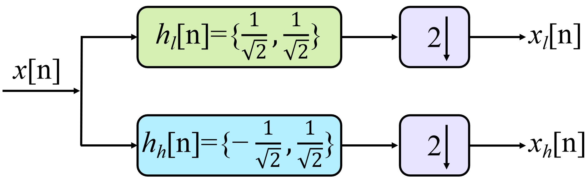
Figure 2: The two-channel Haar filter bank.

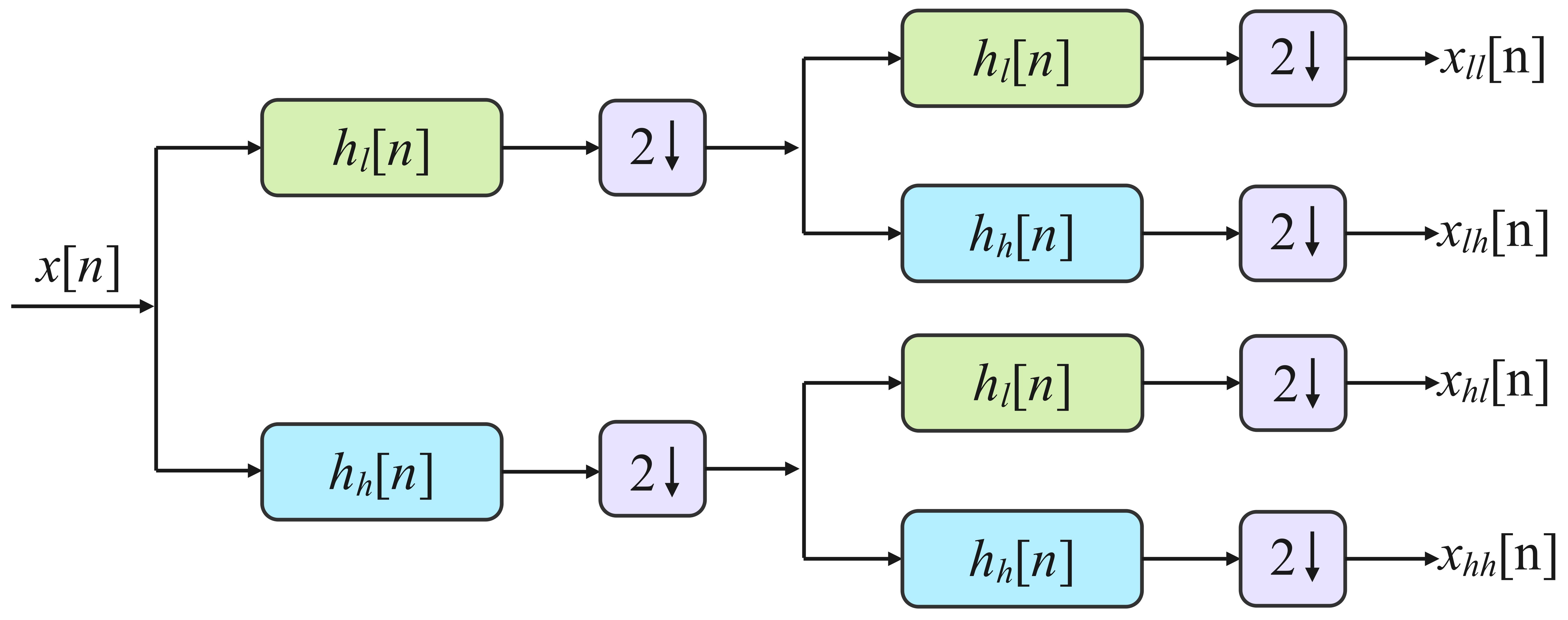
Figure 3: The four-channel Haar filter bank.

Let $x[n]=\{\cdots,x_{0},x_{1},x_{2},x_{3},x_{0},x_{1},x_{2},x_{3},\cdots\}$ is a periodic extension of $\{x_{0},x_{1},x_{2},x_{3}\}$. We have

$$\begin{aligned} &x_{ll}[n]=\{\cdots,\frac{x_{0}+x_{1}+x_{2}+x_{3}}{2},\frac{x_{0}+x_{1}+x_{2}+x_{3}}{2},\cdots\}\\ &x_{lh}[n]=\{\cdots,\frac{x_{0}+x_{1}-x_{2}-x_{3}}{2},\frac{x_{0}+x_{1}-x_{2}-x_{3}}{2},\cdots\}\\ &x_{hl}[n]=\{\cdots,\frac{x_{0}-x_{1}+x_{2}-x_{3}}{2},\frac{x_{0}-x_{1}+x_{2}-x_{3}}{2},\cdots\}\\ &x_{hh}[n]=\{\cdots,\frac{x_{0}-x_{1}-x_{2}+x_{3}}{2},\frac{x_{0}-x_{1}-x_{2}+x_{3}}{2},\cdots\}\\ \end{aligned}$$

Therefore,

$$\begin{pmatrix}[r]x_{ll}[0]\\ x_{lh}[0]\\ x_{hl}[0]\\ x_{hh}[0]\end{pmatrix}\\ =\frac{1}{2}\begin{pmatrix}[r]1&1&1&1\\ 1&1&-1&-1\\ 1&-1&1&-1\\ 1&-1&-1&1\\ \end{pmatrix}\begin{pmatrix}[r]x_{0}\\ x_{1}\\ x_{2}\\ x_{3}\end{pmatrix}\\$$ (25)

where the matrix establishing the relationship between input and output has the same rows as the $4\times 4$ Hadamard transform. Therefore, the last two rows in the Hadamard matrix can be considered as “high-pass filters” to extract the high-frequency components, e.g., noise. Similarly, $8\times 8$ Hadamard transform can be constructed from a $\log_{2}8=3$ layers two-channel filter bank. Then, the last four rows in the Hadamard matrix can be considered as “high-pass filters”. The concept can be generalised to $N$ by $N$ Hadamard transform which can be constructed using a basic two-channel Haar filter bank. Moreover, it is observed that the Hadamard transform requires the size of the input to be a power of 2. However, the signal received by the BS can be of arbitrary size. To solve this problem, we divide $\mathbf{y}_{t}$ into short-time windows of length 8. If the size of the signal is not a multiple of 8, zeros will be padded at the end of the signal.

Although the last half row vectors in the Hadamard matrix work as high-pass filters, these row vectors may not be the optimal choice. Inspired by this, we expect to use more efficient high-pass filters to replace the last half rows in the Hadamard matrix. At present, the derivative operator has been widely used as a high-pass filter [34, 35]. In the case of RA, the derivative of $\mathbf{y}_{t}[i]$ is defined as follows:

$$\mathbf{y}_{t}^{\prime}[i]=\lim_{\Delta h\rightarrow 0}\frac{\mathbf{y}_{t}[i+\Delta h]-\mathbf{y}_{t}[i]}{\Delta h}.$$ (26)

For a discrete signal, the smallest interval $\Delta h$ is 1. Therefore, the derivative is calculated as $\mathbf{y}_{t}[i+1]-\mathbf{y}_{t}[i]$. Similarly, we have $\mathbf{y}_{t}^{\prime}[i+1]=\mathbf{y}_{t}[i+2]-\mathbf{y}_{t}[i+1]$. Furthermore, the second derivative of $\mathbf{y}_{t}[i]$ can be calculated as:

$$\mathbf{y}_{t}^{\prime\prime}[i] =\mathbf{y}_{t}^{\prime}[i+1]-\mathbf{y}_{t}^{\prime}[i]$$

$$=\mathbf{y}_{t}[i+2]-\mathbf{y}_{t}[i+1]-\mathbf{y}_{t}[i+1]+\mathbf{y}_{t}[i]$$

$$=\mathbf{y}_{t}[i+2]-2\mathbf{y}_{t}[i+1]+\mathbf{y}_{t}[i].$$ (27)

It is observed that calculating the second-order derivative is identical to performing a convolution operation with the filter [1,-2,1]. Additionally, the second-order derivative of $\mathbf{y}_{t}$ represents the high-frequency components in the received signal, which includes the noise. Hence, we replace the last half rows in the Hadamard matrix with the second derivative filter [1,-2,1]. Besides, we shift the filter across different rows to high-pass filter the input vectors as much as possible. In terms of the $8\times 8$ Hadamard transform, we modify the Hadamard matrix as follows:

$$\mathbf{{Q}_{8}}=\begin{pmatrix}[r]1&1&1&1&1&1&1&1\\ 1&-1&1&-1&1&-1&1&-1\\ 1&1&-1&-1&1&1&-1&-1\\ 1&-1&-1&1&1&-1&-1&1\\ 1&-2&1&0&0&0&0&0\\ 0&0&1&-2&1&0&0&0\\ 0&0&0&1&-2&1&0&0\\ 0&0&0&0&0&1&-2&1\\ \end{pmatrix}.$$ (28)

After that, for a block input $\mathbf{x}\in\mathbb{R}^{8}$, the MHT is defined as $\mathbf{y}=\mathbf{{Q}_{8}}\mathbf{x}$. The same structure can be extended to higher dimensions in a straightforward manner. In this paper, we only use $8\times 8$ MHT because a small block size is very helpful in reducing the computation cost and the number of trainable parameters which will be introduced in section IV-B. Furthermore, the small-sized MHT reduces latency due to its low computation cost, especially in a mass RA procedure. Additionally, it is experimentally shown in section V that the MHT has a better capability in separating noise from the main components in the frequency domain compared with the Hadamard transform.

IV-B The block MHT layer

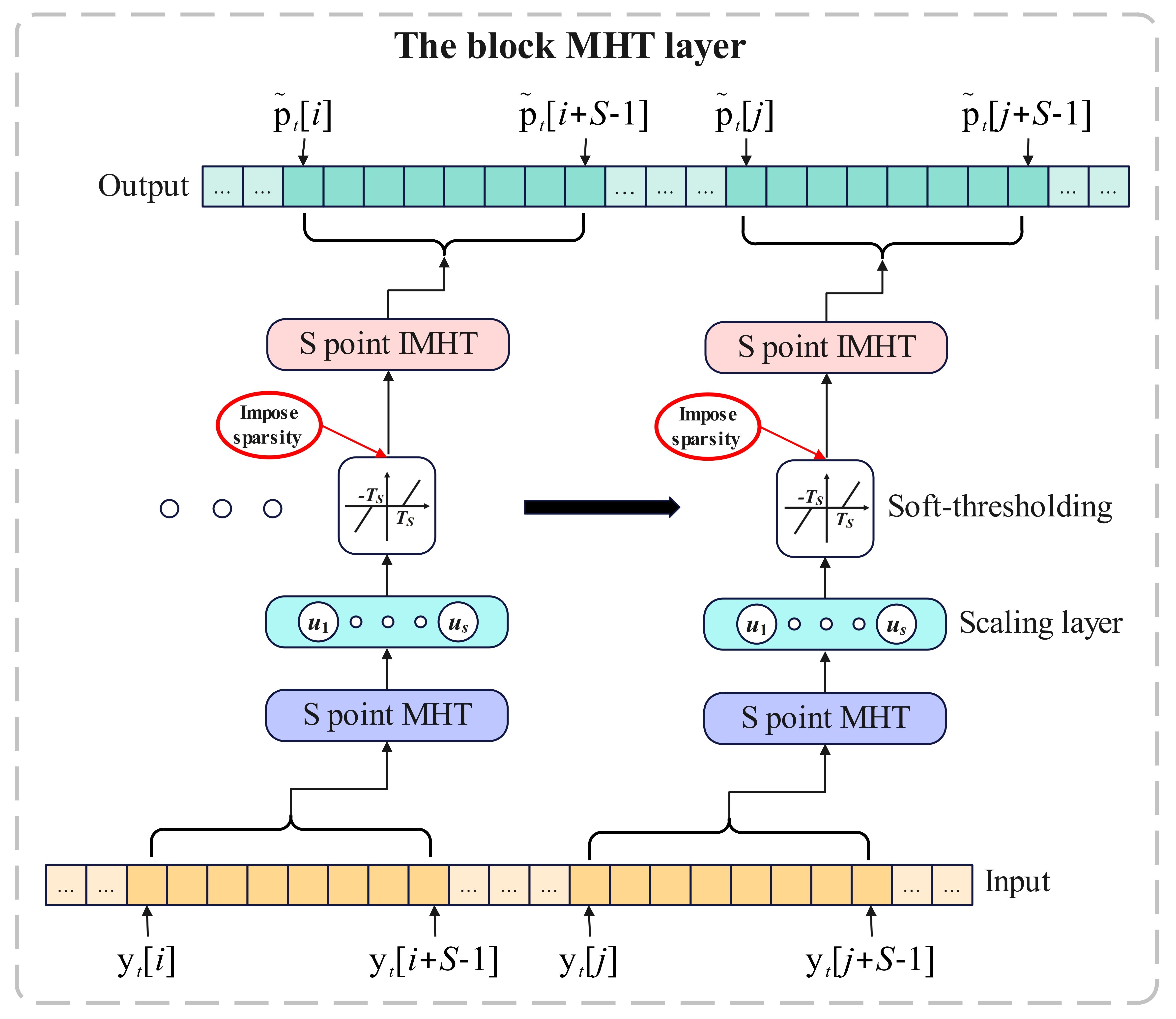
Figure 4: The block MHT layer.

In this section, the block MHT (BMHT) layer is designed to remove the noise from the complex signals $\mathbf{y}_{t}$.

IV-B1 Data preprocessing

we consider the received signal $\mathbf{y}_{t}\in\mathbb{C}^{L}$ on a single antenna as one data sample. Since neural networks cannot be trained with complex numbers, we concatenate the real and imaginary parts of $\mathbf{y}_{t}$ as $\mathbf{y}_{t}^{c}\in\mathbb{R}^{2L}$. Next, we divide $\mathbf{y}_{t}^{c}$ into the small blocks with a size of $S=8$.

IV-B2 Structure of the BMHT layer

as shown in Fig. 4, we first perform the MHT on each input block $\mathbf{\tilde{y}}_{t}\in\mathbb{R}^{S}$. It is computed as:

$$\mathbf{\hat{y}}_{t}=\mathscr{H}(\mathbf{\tilde{y}}_{t})={Q}_{S}\mathbf{\tilde{y}}_{t}.$$ (29)

Then, we employ the scaling layer to allocate weights for different frequency components. It is defined as:

$$\mathbf{\bar{y}}_{t}=\mathbf{\hat{y}}_{t}\circ\mathbf{u},$$ (30)

where $\circ$ represents the element-wise multiplication. $\mathbf{u}\in\mathbb{R}^{S}$ is the scaling vector, which is trained using the back-propagation algorithm [36].

After that, the trainable soft-thresholding layer is utilized to eliminate small entries or scale the large entries in the modified Hadamard domain. The small entries are usually noise and redundant information. The soft-thresholding function is defined as:

$$\mathbf{p}_{t}=\mathcal{S}_{T}\left(\mathbf{\bar{y}}_{t}\right)=\text{sign}\left(\mathbf{\bar{y}}_{t}\right)\cdot\left(|\mathbf{\bar{y}}_{t}|-\mathbf{T}\right)_{+}$$ (31)

where $\mathbf{T}\in\mathbb{R}^{S}$ is the threshold vector trained using the back-propagation algorithm; $(\cdot)_{+}$ stands for the rectified linear unit (ReLU) function. After the soft-thresholding layer, we perform the inverse modified Hadamard transform:

$$\mathbf{\tilde{p}}_{t}=\mathscr{H}^{-1}(\mathbf{p}_{t})=Q_{S}^{-1}\mathbf{p}_{t}.$$ (32)

where

$$Q_{S}^{-1}=\begin{pmatrix}[r]\frac{1}{8}&\frac{5}{8}&\frac{1}{8}&\frac{5}{8}&-\frac{1}{2}&\frac{1}{2}&{1}&{0}\\[1.5pt] \frac{1}{8}&\frac{7}{8}&-\frac{1}{8}&\frac{1}{8}&-{1}&{0}&\frac{1}{2}&\frac{1}{2}\\[1.5pt] \frac{1}{8}&\frac{9}{8}&-\frac{3}{8}&-\frac{3}{8}&-\frac{1}{2}&-\frac{1}{2}&{0}&{1}\\[1.5pt] \frac{1}{8}&\frac{3}{8}&-\frac{1}{8}&-\frac{3}{8}&{0}&-{1}&-\frac{1}{2}&\frac{1}{2}\\[1.5pt] \frac{1}{8}&-\frac{3}{8}&\frac{1}{8}&-\frac{3}{8}&\frac{1}{2}&-\frac{1}{2}&{-1}&{0}\\[1.5pt] \frac{1}{8}&-\frac{9}{8}&\frac{3}{8}&-\frac{3}{8}&{1}&{0}&-\frac{1}{2}&-\frac{1}{2}\\[1.5pt] \frac{1}{8}&-\frac{7}{8}&\frac{1}{8}&\frac{1}{8}&\frac{1}{2}&\frac{1}{2}&{0}&{-1}\\[1.5pt] \frac{1}{8}&-\frac{5}{8}&-\frac{1}{8}&\frac{5}{8}&{0}&{1}&\frac{1}{2}&-\frac{1}{2}\\ \end{pmatrix}$$ (33)

Next, we process the signals block by block. For different blocks, we utilize the same scaling parameters and soft thresholds. Finally, we resize the signal back to its original size by removing the padded zeros.

IV-B3 The training of the BMHT layer

: To eliminate noise and redundant information efficiently, we impose sparsity in the modified Hadamard domain during the training stage. Assume the output of the soft-thresholding layer is $\mathbf{p}_{t}\in\mathbb{R}^{S}$. Then the activity of ${p}_{t,j}$ is computed as:

$$\hat{p}_{t,j}={\sigma}(\mathbf{p}_{t})_{j}=\frac{e^{p_{t,j}}}{e^{p_{t,j}}+1},j=0,1,\cdots,S-1,$$ (34)

where $\sigma(\cdot)$ represents the sigmoid function. Furthermore, the Kullback–Leibler divergence (KLD) [37] has the capability to measure the distinction between the different distributions. Therefore, we employ KLD as the sparsity penalty term:

$$\sum_{j=0}^{S-1}{\rm{KL}}(\kappa||\hat{p}_{t,j})=\sum_{j=0}^{S-1}\kappa\log\frac{\kappa}{\hat{p}_{t,j}}+(1-\kappa)\log\frac{1-\kappa}{1-\hat{p}_{t,j}},$$ (35)

where $\kappa$ is a sparsity parameter. Hence, for each block, the overall loss function $\mathcal{L}$ of the MHT layer is :

$$\mathcal{L}=\frac{1}{S}\sum_{i=0}^{S-1}\left({\bar{p}}_{t,i}-{\tilde{p}}_{t,i}\right)^{2}+\rho\sum_{j=0}^{S-1}{\rm{KL}}\left(\kappa||{\sigma}(\mathbf{p}_{t})_{j}\right),$$ (36)

where $\rho$ is the sparsity penalty weight. ${\tilde{p}}_{t,i}$ and ${\bar{p}}_{t,i}$ stands for the denoised and clean signal on the $t$-th antenna, respectively. Finally, the optimal scaling parameters and soft thresholds are obtained by minimizing the loss function defined in Eq. (36).

IV-C Blind NSVGD algorithm

After the trained BMHT layer denoises the signals, the blind NSVGD algorithm is utilized to perform preamble detection. As mentioned in section III-C, the NSVGD detector requires prior knowledge of the noise power $\delta$ and the number of active devices. However, this prior knowledge is hard to obtain in practical communication scenario. Therefore, this section presents a new blind NSVGD algorithm capable of performing preamble estimation tasks without unknown prior knowledge. As is shown in Algorithm 1, we first initialize the particles $\{\mathbf{x}_{u}\}_{u=1}^{n}$ with a uniform distribution. Next, we start computing $\bigtriangledown_{\mathbf{x}^{r}}\ln g(\mathbf{x}^{r})$. Since $\delta$ is unknown, we remove term $\delta\mathbf{I}$ from $\varphi(\mathbf{x})$ directly. It is feasible because we have performed denoising previously. Then Eq. (14) is rewritten as:

$$\ln g(\mathbf{x})=\ln f(\{\mathbf{y}_{t}\}\mid\mathbf{x})= \sum\limits_{t=1}^{T}-\mathbf{y}_{t}^{\mathrm{H}}(\beta^{2}\mathbf{Z}\mathbf{C}_{\mathbf{x}}\mathbf{Z}^{\mathrm{H}})^{-1}\mathbf{y}_{t}+\eta$$

$$-T\ln\det(\beta^{2}\mathbf{Z}\mathbf{C}_{\mathbf{x}}\mathbf{Z}^{\mathrm{H}}).$$ (37)

Next, $\bigtriangledown_{\mathbf{x}^{r}}\ln g(\mathbf{x}^{r})$ is obtained by computing $\bigtriangledown_{x_{k}^{r}}\ln g(\mathbf{x}^{r})$:

$$\begin{array}[]{l}\bigtriangledown_{\mathbf{x}^{r}}\ln g(\mathbf{x}^{r})=[\bigtriangledown_{x_{1}^{r}}\ln g(\mathbf{x}^{r}),\dots,\bigtriangledown_{x_{K}^{r}}\ln g(\mathbf{x}^{r})].\end{array}$$ (39)

From Eq. (IV-C), $\bigtriangledown_{x_{k}^{r}}\ln g(\mathbf{x}^{r})$ is computed as follows:

$$\bigtriangledown_{x_{k}^{r}}\ln g(\mathbf{x}^{r})= -\bigtriangledown_{x_{k}^{r}}(\sum\limits_{t=1}^{T}\mathbf{y}_{t}^{\mathrm{H}}(\beta^{2}\mathbf{Z}\mathbf{C}_{\mathbf{x}}\mathbf{Z}^{\mathrm{H}})^{-1}\mathbf{y}_{t})$$

$$-\bigtriangledown_{x_{k}^{r}}(T\ln\det(\beta^{2}\mathbf{Z}\mathbf{C}_{\mathbf{x}}\mathbf{Z}^{\mathrm{H}})).$$ (40)

Let $\varepsilon(\mathbf{x})=\beta^{2}\mathbf{Z}\mathbf{C}_{\mathbf{x}}\mathbf{Z}^{\mathrm{H}}$, we have

$$\begin{array}[]{l}\bigtriangledown_{x_{k}^{r}}(\sum\limits_{t=1}^{T}\mathbf{y}_{t}^{\mathrm{H}}\varepsilon(\mathbf{x})^{-1}\mathbf{y}_{t})=\sum\limits_{t=1}^{T}\mathbf{y}_{t}^{\mathrm{H}}\bigtriangledown_{x_{k}^{r}}(\varepsilon(\mathbf{x})^{-1})\mathbf{y}_{t}.\end{array}$$ (42)

From inverse matrix derivative lemma [38], $\bigtriangledown_{x_{k}^{r}}(\varepsilon(\mathbf{x})^{-1})$ is computed as:

$$\bigtriangledown_{x_{k}^{r}}(\varepsilon(\mathbf{x})^{-1})=-\varepsilon(\mathbf{x})^{-1}\bigtriangledown_{x_{k}^{r}}(\varepsilon(\mathbf{x}))\varepsilon(\mathbf{x})^{-1},$$ (43)

where

$$\begin{array}[]{l}\bigtriangledown_{x_{k}^{r}}(\varepsilon(\mathbf{x}))=\beta^{2}\mathbf{z}_{k}\mathbf{z}_{k}^{\mathrm{H}}.\end{array}$$ (45)

From Eq. (43) and Eq. (45), Eq. (42) is rewritten as:

$$\begin{aligned} \bigtriangledown_{x_{k}^{r}}(\sum\limits_{t=1}^{T}\mathbf{y}_{t}^{\mathrm{H}}\varepsilon(\mathbf{x})^{-1}\mathbf{y}_{t})=-\beta^{2}\sum_{t=1}^{T}\mathbf{y}_{t}^{\mathrm{H}}\varepsilon(\mathbf{x})^{-1}\mathbf{z}_{k}\mathbf{z}_{k}^{\mathrm{H}}\varepsilon(\mathbf{x})^{-1}\mathbf{y}_{t}\end{aligned}$$ (46)

At the next step, $\bigtriangledown_{x_{k}^{r}}(T\ln\det(\varepsilon(\mathbf{x})))$ is calculated as:

$$\bigtriangledown_{x_{k}^{r}}(T\ln\det(\varepsilon(\mathbf{x}))) =T\bigtriangledown_{x_{k}^{r}}(\ln\det(\varepsilon(\mathbf{x})))$$

$$=\frac{T}{\det(\varepsilon(\mathbf{x}))}\bigtriangledown_{x_{k}^{r}}(\det(\varepsilon(\mathbf{x}))).$$ (47)

Applying the matrix determinant derivative lemma [38], we obtain:

$$\begin{array}[]{l}\bigtriangledown_{x_{k}^{r}}(\det(\varepsilon(\mathbf{x})))=\det(\varepsilon(\mathbf{x})){\rm{tr}}(\varepsilon(\mathbf{x})^{-1}\bigtriangledown_{x_{k}^{r}}(\varepsilon(\mathbf{x}))).\end{array}$$ (49)

From Eq. (IV-C) and Eq. (49), we have

$$\begin{array}[]{l}\bigtriangledown_{x_{k}^{r}}(T\ln\det(\varepsilon(\mathbf{x})))=T\cdot{\rm{tr}}{(\varepsilon(\mathbf{x})^{-1}\beta^{2}\mathbf{z}_{k}\mathbf{z}_{k}^{\mathrm{H}})}.\end{array}$$ (51)

Finally, we have:

$$\bigtriangledown_{x_{k}^{r}}\ln g(\mathbf{x}^{r})= \beta^{2}\sum_{t=1}^{T}{\mathbf{y}_{t}}^{\mathrm{H}}\varepsilon(\mathbf{x})^{-1}\mathbf{z}_{k}\mathbf{z}_{k}^{\mathrm{H}}\varepsilon(\mathbf{x})^{-1}\mathbf{y}_{t}$$

$$-T\cdot{\rm{tr}}{(\varepsilon(\mathbf{x})^{-1}\beta^{2}{\mathbf{z}_{k}}{\mathbf{z}_{k}}^{\mathrm{H}})}.$$ (52)

After computing $\bigtriangledown_{x_{k}^{r}}\ln g(\mathbf{x}^{r})$, we update the gradient according to Eq. (17). Next, the history gradients are accumulated. Then, the accumulated gradient is normalized as follows:

$${\omega}(\mathbf{x}_{u}^{r})\leftarrow\frac{{\omega}(\mathbf{x}_{u}^{r})}{\epsilon+\sqrt{\mathbf{q}_{r}}},$$ (53)

where $\epsilon$ is a constant and $\sqrt{(\cdot)}$ stands for element-wise square root. These operations address the issue of the learning rate continually decreasing compared to the AdaGrad method [39]. Moreover, we employ weight decay [40] and momentum strategy [41] to optimize the gradient ${\omega}(\mathbf{x}_{u}^{r})$ as shown in Algorithm 1. Finally, the particles are updated according to Eq. (16). After numerous iterations, the particles $\{\mathbf{\hat{x}}_{u}\}_{u=1}^{n}$ sampled by the blind NSVGD algorithm are employed to estimate the number of devices choosing each preamble. For example, as shown in Fig. 5, we have six active devices and six preambles in the cell. At first, ten particles are initialized using random numbers. As the number of iterations increases, the particles gradually approach the ground truth. After 1000 iterations, the particles converge to the ground truth.

It is observed that the blind NSVGD algorithm performs preamble detection without using the information of noise power and the number of active devices compared with the NSVGD detector. This is because we apply the BMHT layer to denoise the complex signals before detecting preambles, which mitigates the vanishing gradients problem in the SVGD detector discussed in section III-C. Therefore, we do not need to introduce any bias correction term to provide extra information to update the particles. The process of the blind NSVGD-based detector is summarized in Algorithm 1.

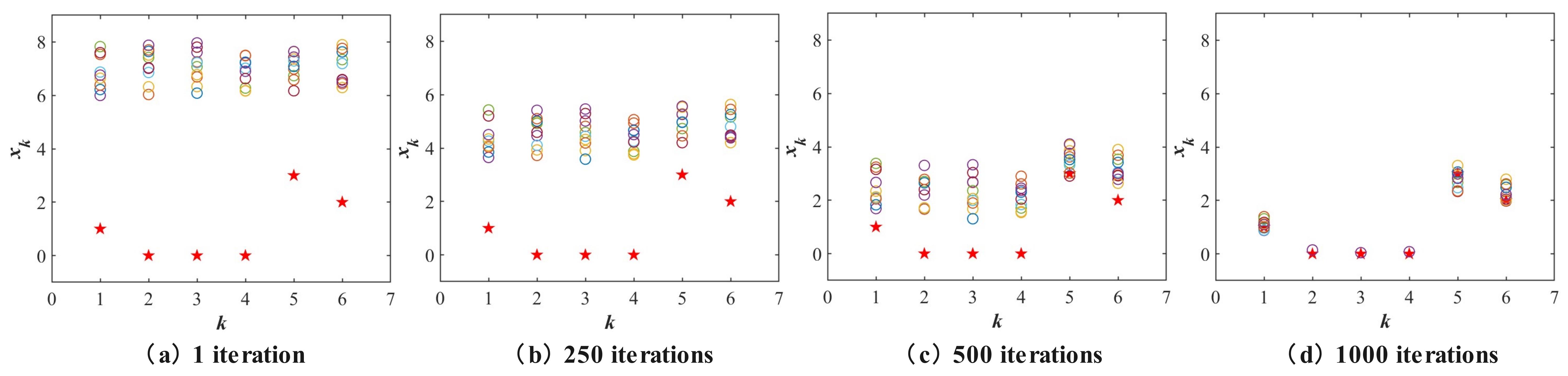
Figure 5: Updating process of particles. The circles represent particles and the pentagrams represent ground truth. $k$ is the index of the preamble and $x_{k}$ is the number of devices choosing $k$-th preamble. $K=6$, $L=6$, $M=6$, $T=20$, and $\rm{SNR}=16$ dB.

Input: The received signals $\{\mathbf{y}_{t}^{c}\}_{t=1}^{T}$, a target function $g(\mathbf{x})$ and the initial particles $\{\mathbf{x}_{u}^{0}\}_{u=1}^{n}$

Output: A set of particles $\{\hat{\mathbf{x}}_{u}\}_{u=1}^{n}$ that approximates the target function

/* Denoising stage */

1 Divide $\{\mathbf{y}_{t}^{c}\}_{t=1}^{T}$ into $S$-length short-time windows.

2for block i do

3      

4      Perform the MHT using Eq. (29).

5      Remove the noise using Eq. (30) and Eq (31).

6      Perform the IMHT using Eq. (32).

7 end for

/* Preamble detection stage */

8 for iteration $r$ do

9      

10      Compute $\bigtriangledown_{x_{k}^{r}}\ln g(\mathbf{x}^{r})$ using Eq. (IV-C).

11      Update ${\omega}(\mathbf{x}_{u}^{r})$ according to Eq. (17).

      /* Accumulate history gradients */

12       if $\varrho\neq 0$ then

13             if $r>1$ then

14                   ${\mathbf{q}}_{r}\leftarrow\varrho{\mathbf{q}}_{r-1}+(1-\varrho){\omega}^{2}(\mathbf{x}_{u}^{r})$

15             else

16                  ${\mathbf{q}}_{r}\leftarrow{\omega}^{2}(\mathbf{x}_{u}^{r})$

17             end if

18            

19       end if

20      

21      Calculate ${\omega}(\mathbf{x}_{u}^{r})$ using Eq. (53).

      /* Weight Decay */

22       if $\gamma\neq 0$ then

23             ${\omega}(\mathbf{x}_{u}^{r})\leftarrow{\omega}(\mathbf{x}_{u}^{r})-\gamma\mathbf{x}_{u}^{r}$

24       end if

25      

      /* Gradient with Momentum */

26       if $\alpha\neq 0$ then

27             if $r>1$ then

28                   ${\mathbf{b}}_{r}\leftarrow\alpha{\mathbf{b}}_{r-1}+(1-\alpha){\omega}(\mathbf{x}_{u}^{r})$

29             else

30                  ${\mathbf{b}}_{r}\leftarrow{\omega}(\mathbf{x}_{u}^{r})$

31             end if

32            ${\omega}(\mathbf{x}_{u}^{r})\leftarrow{\mathbf{b}}_{r}$

33       end if

34      

35      Compute $\mathbf{x}_{u}^{r+1}$ using Eq. (16).

36 end for

Algorithm 1 Blind NSVGD-Based Detector

V Experimental Results

In the experimental section, we present the simulation results to explore the effectiveness of the algorithms proposed in our study. Specifically, to validate the denoising performance of the block MHT layer, other transform domain layers are selected as comparison models such as the DCT layer [24], block wavelet transform perceptron (BWTP) layer [42] and Hadamard Transform Perceptron (HTP) layer [26]. In the HTP layer, we set the number of channels as 3. Besides, the convolutional neural network (CNN) [43] and sparse autoencoder (AE) [37] are also utilized as comparison benchmarks because the convolutional and linear layers are widely employed for the denoising tasks. Additionally, to verify the preamble detection performance of the blind NSVGD-based detector, we choose other approximate inference-based detectors as comparison models, such as the MCMC detector [19], SVGD detector [20] and NSVGD detector [20].

In the experiments, we mainly consider a dense device scenario by setting $K=M$ because our target is to detect preamble collision. Besides, since the noise power $\delta$ and the number of active users $M$ are unknown in the practical communication scenarios, all detectors perform preamble detection without using the information of $\delta$ and $M$. Additionally, for all SVGD-based detectors, the particles $\{x_{u}\}_{u=1}^{n}$ are initialized using a uniform distribution on $[1,1.1]$. Then, the parameters $n$, $\beta$, $\lambda$, ${\kappa}$, $\rho$, $\epsilon$, and $\gamma$ are chosen as 6, 1, 0.01, 0.001, 0.5, 1, and 0.1, respectively. Suppose $N$ denotes the number of iterations required to achieve stable particles. The sample mean of the particles is computed as:

$$\bar{\mathbf{x}}=\frac{1}{n}\sum_{u=1}^{n}\hat{\mathbf{x}}_{u}=[\bar{x}_{0},\dots,\bar{x}_{k},\dots,\bar{x}_{K}].$$ (54)

Then, $\tilde{x}_{k}$ is estimated by the rounded sample mean, i.e., $\tilde{x}_{k}=\lfloor\bar{x}_{k}\rceil\in\{0,\dots,M\}$, where $\lfloor x\rceil$ is the nearest integer of $x$.

V-A Performance metrics

To evaluate the denoising performance of different methods, the percent root mean square difference (PRD) and root mean square (RMS) are employed. RMS measures the distinctions between the clean signal and the denoised signal.

$${\rm{RMS}}=\sqrt{\frac{1}{w}\sum_{i=0}^{w-1}\left(s_{i}^{c}-s_{i}^{d}\right)^{2}},$$ (55)

where $w$ is the length of the signal. $s_{i}^{c}$ is the clean signal. $s_{i}^{d}$ is the denoised signal. The lower the RMS is, the better denoising performance the approach has.

PRD evaluates the distortion of the denoised signal:

$${\rm{PRD}}=\sqrt{\frac{\sum_{i=0}^{w-1}\left(s_{i}^{c}-s_{i}^{d}\right)^{2}}{\sum_{i=0}^{w-1}\left(s_{i}^{c}\right)^{2}}}.$$ (56)

The lower the PRD is, the better the model is.

Moreover, we utilize two performance metrics to evaluate the accuracy of the proposed preamble detection algorithm. Firstly, we consider the mean squared error (MSE). The MSE measures the difference between the true values and the estimated values. It is defined as follows:

$${\rm{MSE}}(x_{k})=\mathbb{E}(x_{k}-\tilde{x}_{k})^{2}.$$ (57)

The lower the MSE is, the higher the accuracy of the preamble detection is.

Another performance metric is the probability of activity detection error, which reflects the average proportion of incorrectly estimated preambles. It is defined as:

$$\begin{array}[]{l}{\rm{P_{ADE}}}={\rm{Pr}}(x_{k}\neq\tilde{x}_{k}).\end{array}$$ (59)

The lower the $\rm{P_{ADE}}$ is, the higher the accuracy of the preamble detection is.

Additionally, $N_{p}$ represents the number of trainable parameters. The Multiply–Accumulates (MACs) are employed to evaluate the computation complexity. One MAC represents one addition and one multiplication.

V-B Denoising Experiment

In the denoising experiment, we generate a dataset using the signal reception model defined in Eq. (1). Specifically, we generate 3000 noisy samples as inputs and corresponding clean samples as labels by setting $K=20$, $L=10$, $M=20$ and $\rm{SNR}=12$ dB. These data samples are employed as training datasets. Furthermore, to test the generalization capability of denoising models, another 3000 sample pairs are generated as testing datasets by changing $\rm{SNR}$ to 8 dB. Additionally, during the training stage, we use the AdamW optimizer [44]. The learning rate and batch size are set as 0.001 and 128 respectively.

Table I presents the denoising results of different models on the testing datasets. Compared with CNN, the BMHT layer reduces RMS from 34.61 to 27.38 (20.89%) and PRD from 34.56 to 27.34 (20.89%). Additionally, $N_{p}$ decreases from 824 to 16 (98.06%) and MACs decreases from 840 to 216 (74.29%). Although CNN applies more trainable parameters than the BMHT layer, the BMHT layer still achieves a better denoising performance than CNN. It indicates too many training parameters can result in overfitting of the model. Moreover, the sparse AE and the BMHT layer both use the penalty term to reduce noise. However, the BMHT layer outperforms the sparse AE in terms of RMS, PRD and MACs. It experimentally shows that the transform-based method is more efficient than the linear-based method. Additionally, the BMHT layer is superior to other familiar transform-based models such as the DCT layer, BWTP layer and HTP layer because of a lower RMS and PRD. The reason is that the KL divergence-based sparsity penalty is applied in the BMHT layer to keep latent space sparse, which helps remove noise in the transform domain. Besides, in comparison to the HTP layer, no convolutional layers are implemented in the BMHT layer, which reduces the computation costs and number of parameters.

The ablation experiments are used to validate the function of each module in the BMHT layer. As shown in Table II, when the scaling layer is removed, the denoising performance degrades as the RMS increases from 27.38 to 28.04 (2.41%) and PRD from 27.34 to 27.99 (2.38%). This is because the scaling layer is capable of assigning appropriate emphasis to frequency domain components. Additionally, when the sparsity penalty and soft thresholding layer are not present in the BMHT layer, the RMS and PRD both increase. It shows that the penalty term and soft threshold are beneficial to retaining important features and eliminating redundant information such as noise. Furthermore, it is observed that the RMS and PRD increase when the MHT is replaced with the standard Hadamard transform (HT). Therefore, it is experimentally shown that the MHT has a better ability to separate the noise from the important components than the standard Hadamard transform.

TABLE I: Denoising Experimental Results.

Method	$N_{p}$	MACs	RMS (%)	PRD (%)
CNN	824	840	34.61	34.56
DCT Layer	40	820	27.48	27.44
Sparse AE	676	640	47.59	47.52
BWTP Layer	51	550	27.48	27.44
HTP Layer	195	1216	27.48	27.44
BMHT LAYER	16	216	27.38	27.34

TABLE II: Ablation study.

Method	$N_{p}$	MACs	RMS (%)	PRD (%)
No penalty	16	216	27.47	27.43
No scaling	8	192	28.04	27.99
No threshold	8	216	27.49	27.44
Standard HT	16	216	27.85	27.81
BMHT LAYER	16	216	27.38	27.34

V-C Preamble Detection Experiments

In the preamble detection experiments, to test the generalization ability of the proposed model, we use the fixed BMHT layer which is trained when $K=20$, $L=10$, $M=20$ and $\rm{SNR}=12$ dB. It means that even if $K$, $M$ and $\rm{SNR}$ change in the environment, we do not train the BMHT layer again.

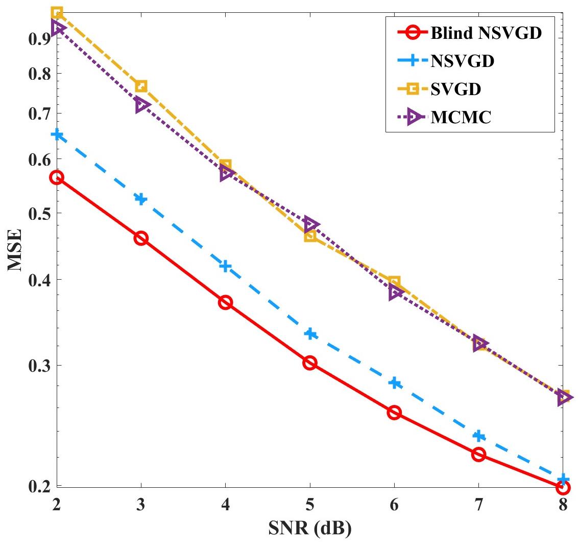
Figure 6: MSE for different SNR when $K=20$, $L=10$, $M=20$ and $T=30$.

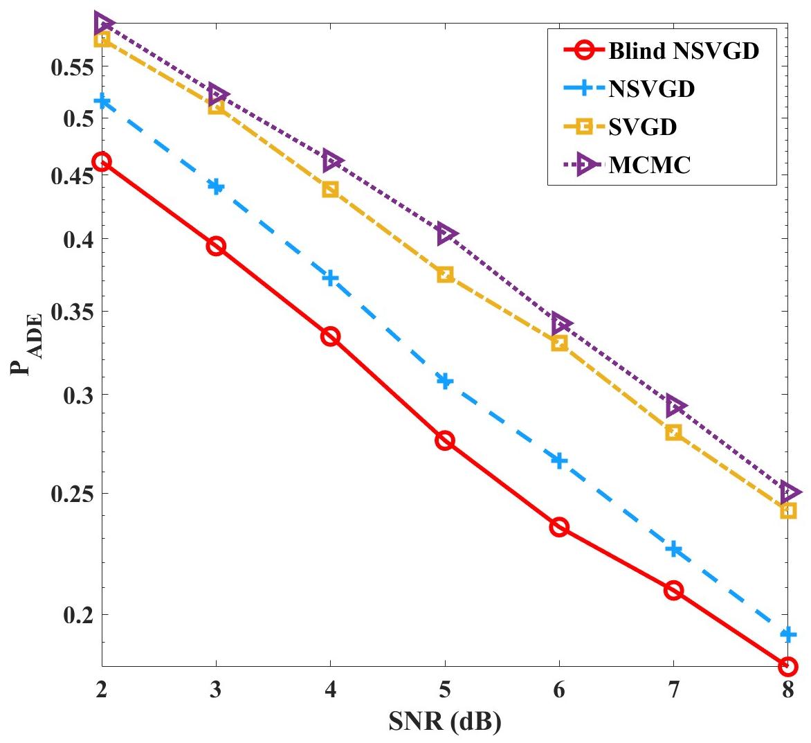
Figure 7: $\rm{P_{ADE}}$ for different SNR when $K=20$, $L=10$, $M=20$ and $T=30$.

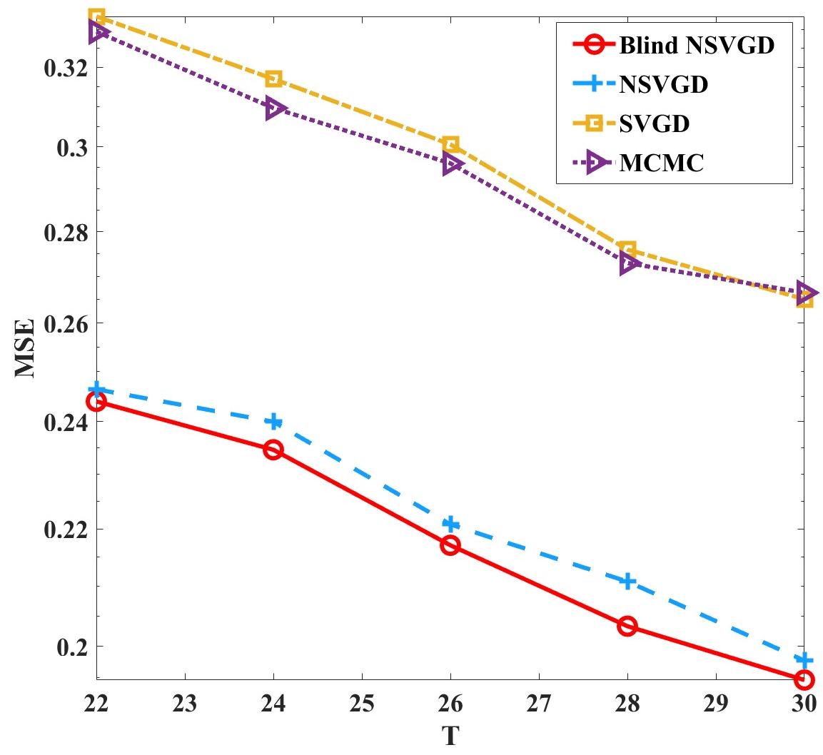
Figure 8: MSE for different numbers of $T$ when $K=20$, $L=10$, $M=20$ and $\rm{SNR}=8$ dB.

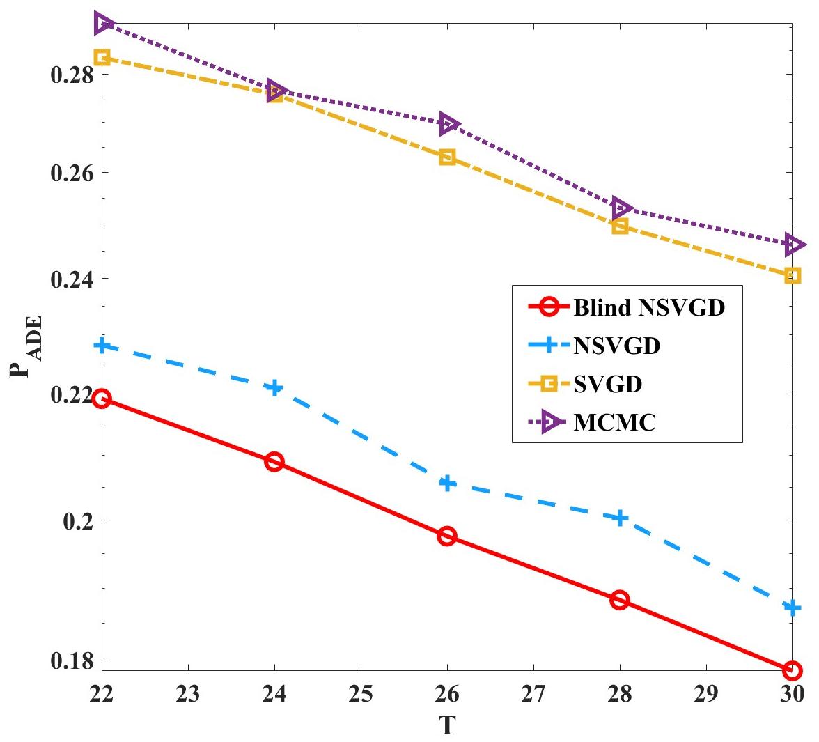
Figure 9: $\rm{P_{ADE}}$ for different numbers of $T$ when $K=20$, $L=10$, $M=20$ and $\rm{SNR}=8$ dB.

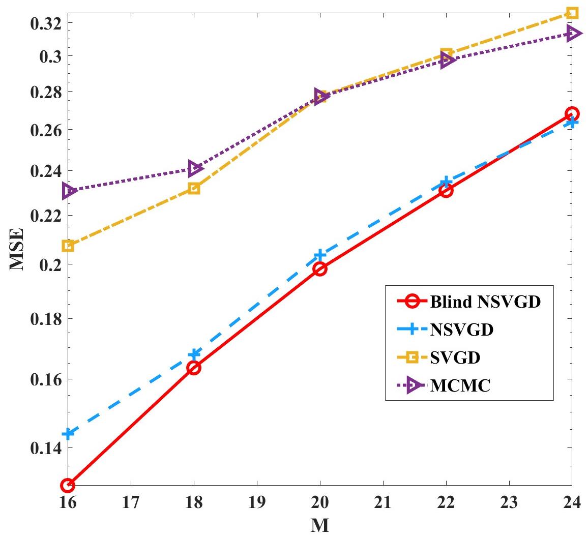
Figure 10: MSE for different numbers of active devices when $K=20$, $L=10$, $T=30$ and $\rm{SNR}=8$ dB.

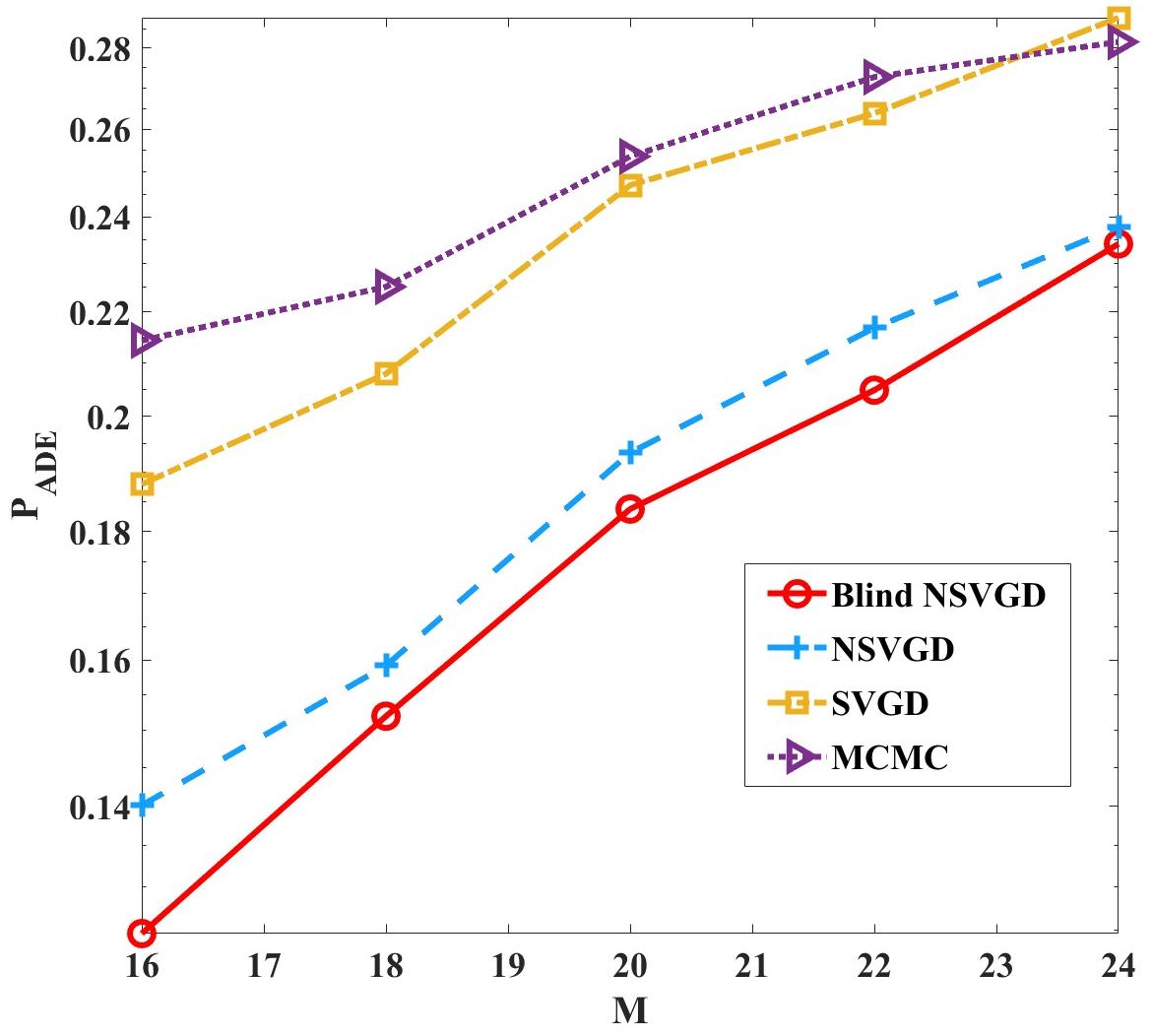
Figure 11: $\rm{P_{ADE}}$ for different numbers of active devices when $K=20$, $L=10$, $T=30$ and $\rm{SNR}=8$ dB.

Fig. 6 and Fig. 7 show the preamble detection performance of four models at different SNR. As the SNR increases, the MSE and $\rm{P_{ADE}}$ of each model decrease, which indicates an improvement in detection accuracy. It is observed that the blind NSVGD-based detector surpasses the MCMC, SVGD and NSVGD detectors in terms of MSE and $\rm{P_{ADE}}$. Additionally, when the SNR is 8 dB, the proposed method exhibits a small performance improvement over the NSVGD detector. It is because there is a small noise in the environment when SNR is high. However, as SNR decreases, the performance gap between the proposed method and the NSVGD detector also widens. When SNR is 4 dB, compared with the NSVGD detector, the proposed detector reduces MSE from 0.4185 to 0.3703 (9.61%) and $\rm{P_{ADE}}$ from 0.3721 to 0.3340 (10.24%). The reason is that the BMHT layer achieves good denoising performance under low SNR. Therefore, the blind NSVGD-based detector can extract more efficient gradient information to update the particles without prior knowledge of active devices and noise power.

Fig. 8 and Fig. 9 show the effect of different numbers of antennas on the MSE and $\rm{P_{ADE}}$. With the number of antennas increasing, both the MSE and $\rm{P_{ADE}}$ decrease, leading to a continuous reduction in preamble detection error. This is because more antennas introduce diversity in receiving signals, which alleviates noise and fading. Additionally, the performance of the blind NSVGD-based detector remains superior to that of the MCMC, NSVGD and SVGD detectors. It indicates that the proposed detector has better robustness than other baselines.

In Fig. 10 and Fig. 11, we show the performances of the MCMC, SVGD, NSVGD and the blind NSVGD-based detectors for different numbers of active devices. When the number of active devices increases, the MSE and $\rm{P_{ADE}}$ both increase. The reason is that the number of preamble collisions increases when more active devices try to access to network simultaneously. Severe preamble collisions bring much interference, which makes it difficult for approximate inference-based methods to perform preamble detection. Additionally, the blind NSVGD-based detector still outperforms other detectors under different $M$, which indicates the proposed method can achieve good results in both sparse and dense device scenarios.

Fig. 12 compares the throughputs of different detectors. Throughput refers to the average count of successfully accessed preambles, excluding instances of collisions and false detections. As $M$ increases, the throughputs of different detectors decrease. One reason for this is that the preamble collisions rise with the active devices increasing, leading to a decrease in the number of successfully accessed devices. Moreover, when $M=24$, compared with the SVGD detector, the blind NSVGD-based detector achieves a significant performance improvement as it increases throughput from 5.16 to 6.01 (16.47%). Moreover, the blind NSVGD-based detector also performs better than the NSVGD detector. It indicates even when severe preamble collisions happen, the proposed detector still can achieve higher accuracy in detecting the successfully accessed preambles.

V-D The analysis of computational complexity

The computation complexities of the MCM detector, SVGD detector and NSVGD detector are $O(KL(L+T))$, $O(KTL^{3})$ and $O(KTL^{3})$ respectively [20, 19]. Additionally, compared with the NSVGD detector, the blind NSVGD-based detector introduces the extra computation cost of the BMHT layer. The computation complexity of the BMHT layer is $O(L)$. Therefore it can be omitted compared with $O(KTL^{3})$. Finally, the overall complexity of the blind NSVGD-based detector is $O(KTL^{3})$. Hence, given a fixed $L$, the complexities of all detectors are linearly proportional to $K$ and $T$. Additionally, they are independent of the number of active users.

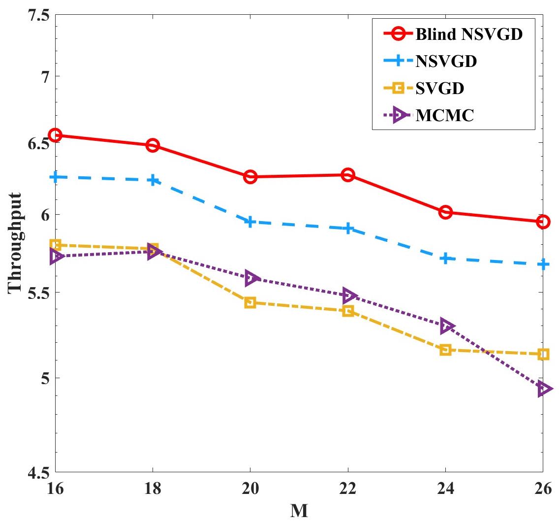
Figure 12: Throughput for different numbers of active devices when $K=20$, $L=10$, $T=30$ and $\rm{SNR}=8$ dB.

VI Conclusion

In this paper, to reduce resource wastage, we proposed an early preamble detection scheme based on the blind NSVGD-based detector at the first step of the grant-based RA scheme. The blind NSVGD-based detector consist of two modules: a BMHT layer and a blind NSVGD algorithm. At the receiver, the MHT was first conceived. It separated the high frequencies from the signal in the transform domain. After that, the BMHT layer was designed based on the MHT, trainable scaling layer and soft-thresholding layer. It removed the noise and alleviated the issue of vanishing gradients in the SVGD-based detectors. Finally, the derived blind NSVGD algorithm finished the preamble detection task without requiring unknown prior knowledge. The simulation results demonstrated the BMHT layer outperformed other denoising methods with a low computation cost. Additionally, aided by the BMHT layer, the proposed detector had a consistent performance improvement over the MCMC detector and other SVGD-based detectors in terms of detection accuracy and throughput.

References

- [1] Chin-Wei Hsu and Hun-Seok Kim, “Hyper-dimensional modulation for robust short packets in massive machine-type communications,” IEEE Transactions on Communications, vol. 71, no. 3, pp. 1388–1402, 2023.
- [2] Zhe Ma, Wen Wu, Feifei Gao, and Xuemin Shen, “Model-driven deep learning for non-coherent massive machine-type communications,” IEEE Transactions on Wireless Communications, 2023.
- [3] Feng Ye, Jiamin Li, Pengcheng Zhu, Dongming Wang, and Xiaohu You, “Density-based clustering resolution for grant-free preamble collision in cell-free murllc systems,” IEEE Transactions on Vehicular Technology, 2023.
- [4] Jinho Choi, Jie Ding, Ngoc-Phuc Le, and Zhiguo Ding, “Grant-free random access in machine-type communication: Approaches and challenges,” IEEE Wireless Communications, vol. 29, no. 1, pp. 151–158, 2021.
- [5] Yi Yin, Dongmei Zhao, Xufei Li, and Shuiguang Zeng, “Learning based preamble collision detection of cellular random access by physical layer features,” in 2023 International Conference on Networking and Network Applications (NaNA). IEEE, 2023, pp. 28–33.
- [6] Iqbal H Sarker, Asif Irshad Khan, Yoosef B Abushark, and Fawaz Alsolami, “Internet of things (IoT) security intelligence: A comprehensive overview, machine learning solutions and research directions,” Mobile Networks and Applications, vol. 28, no. 1, pp. 296–312, 2023.
- [7] Abdullah Balcı and Radosveta Sokullu, “Fairness aware deep reinforcement learning for grant-free noma-iot networks,” Internet of Things, p. 101079, 2024.
- [8] Monowar Hasan, Ekram Hossain, and Dusit Niyato, “Random access for machine-to-machine communication in lte-advanced networks: Issues and approaches,” IEEE communications Magazine, vol. 51, no. 6, pp. 86–93, 2013.
- [9] Yeduri Sreenivasa Reddy, Ankit Dubey, Abhinav Kumar, and Trilochan Panigrahi, “A successive interference cancellation based random access channel mechanism for machine-to-machine communications in cellular internet-of-things,” IEEE Access, vol. 9, pp. 8367–8380, 2021.
- [10] Níbia Souza Bezerra, Min Wang, Christer Åhlund, Mats Nordberg, and Olov Schelén, “Rach performance in massive machine-type communications access scenario,” in 2018 IEEE Wireless Communications and Networking Conference (WCNC). IEEE, 2018, pp. 1–6.
- [11] Kaijie Zhou and Navid Nikaein, “Low latency random access with tti bundling in LTE/LTE-A,” in 2015 IEEE International Conference on Communications (ICC). IEEE, 2015, pp. 2257–2263.
- [12] Ya-Feng Liu, Wei Yu, Ziyue Wang, Zhilin Chen, and Foad Sohrabi, “Grant-free random access via covariance-based approach,” Next Generation Multiple Access, pp. 391–414, 2024.
- [13] Xinyu Bian, Yuyi Mao, and Jun Zhang, “Joint activity detection, channel estimation, and data decoding for grant-free massive random access,” IEEE Internet of Things Journal, 2023.
- [14] Chung G Kang, Ameha Tsegaye Abebe, and Jinho Choi, “Noma-based grant-free massive access for latency-critical internet of things: A scalable and reliable framework,” IEEE Internet of Things Magazine, vol. 6, no. 3, pp. 12–18, 2023.
- [15] Liang Liu, Erik G Larsson, Wei Yu, Petar Popovski, Cedomir Stefanovic, and Elisabeth De Carvalho, “Sparse signal processing for grant-free massive connectivity: A future paradigm for random access protocols in the internet of things,” IEEE Signal Processing Magazine, vol. 35, no. 5, pp. 88–99, 2018.
- [16] Jiaai Liu and Xiaodong Wang, “A grant-based random access scheme with low latency for mmtc in iot networks,” IEEE Internet of Things Journal, 2023.
- [17] Han Seung Jang, Su Min Kim, Hong-Shik Park, and Dan Keun Sung, “An early preamble collision detection scheme based on tagged preambles for cellular M2M random access,” IEEE Transactions on Vehicular Technology, vol. 66, no. 7, pp. 5974–5984, 2016.
- [18] Li Zhen, Yukun Zhang, Keping Yu, Neeraj Kumar, Ahmed Barnawi, and Yongbin Xie, “Early collision detection for massive random access in satellite-based internet of things,” IEEE Transactions on Vehicular Technology, vol. 70, no. 5, pp. 5184–5189, 2021.
- [19] Jinho Choi, “MCMC-based detection for random access with preambles in MTC,” IEEE Transactions on Communications, vol. 67, no. 1, pp. 835–846, 2018.
- [20] Xin Zhu, Hongyi Pan, Salih Atici, and Ahmet Enis Cetin, “Stein variational gradient descent-based detection for random access with preambles in mtc,” arXiv preprint arXiv:2309.08782, 2023.
- [21] Jie Ni and Jianping Zheng, “Index modulation-based non-coherent transmission in grant-free massive access,” IEEE Transactions on Vehicular Technology, vol. 70, no. 1, pp. 1025–1029, 2020.
- [22] Muhammad Usman Khan, Enrico Testi, Enrico Paolini, and Marco Chiani, “Preamble detection in asynchronous random access using deep learning,” IEEE Wireless Communications Letters, 2023.
- [23] Valentin Mikhailov, Nikita Stepanov, and Andrey Turlikov, “Performance assessment of an early preamble collision detection approach for cellular m2m random access,” in 2023 XVIII International Symposium Problems of Redundancy in Information and Control Systems (REDUNDANCY). IEEE, 2023, pp. 30–34.
- [24] Hongyi Pan, Xin Zhu, Zhilu Ye, Pai-Yen Chen, and Ahmet Enis Cetin, “Real-time wireless ecg-derived respiration rate estimation using an autoencoder with a dct layer,” in ICASSP 2023-2023 IEEE International Conference on Acoustics, Speech and Signal Processing (ICASSP). IEEE, 2023, pp. 1–5.
- [25] Hongyi Pan, Diaa Badawi, Chang Chen, Adam Watts, Erdem Koyuncu, and Ahmet Enis Cetin, “Deep neural network with walsh-hadamard transform layer for ember detection during a wildfire,” in Proceedings of the IEEE/CVF Conference on Computer Vision and Pattern Recognition, 2022, pp. 257–266.
- [26] Hongyi Pan, Xin Zhu, Salih Furkan Atici, and Ahmet Cetin, “A hybrid quantum-classical approach based on the hadamard transform for the convolutional layer,” in International Conference on Machine Learning. PMLR, 2023, pp. 26891–26903.
- [27] Xin Zhu, Daoguang Yang, Hongyi Pan, Hamid Reza Karimi, Didem Ozevin, and Ahmet Enis Cetin, “A novel asymmetrical autoencoder with a sparsifying discrete cosine stockwell transform layer for gearbox sensor data compression,” Engineering Applications of Artificial Intelligence, vol. 127, pp. 107322, 2024.
- [28] Qiang Liu and Dilin Wang, “Stein variational gradient descent: A general purpose bayesian inference algorithm,” Advances in Neural Information Processing Systems, vol. 29, 2016.
- [29] Qiang Liu, Jason Lee, and Michael Jordan, “A kernelized Stein discrepancy for goodness-of-fit tests,” in International Conference on Machine Learning. PMLR, 2016, pp. 276–284.
- [30] Qian Zhao, Hui Wang, Xuehu Zhu, and Deyu Meng, “Stein variational gradient descent with learned direction,” Information Sciences, vol. 637, pp. 118975, 2023.
- [31] N Nüsken, “On the geometry of stein variational gradient descent,” Journal of Machine Learning Research, vol. 24, pp. 1–39, 2023.
- [32] Bor-Chen Kuo, Hsin-Hua Ho, Cheng-Hsuan Li, Chih-Cheng Hung, and Jin-Shiuh Taur, “A kernel-based feature selection method for SVM with RBF kernel for hyperspectral image classification,” IEEE Journal of Selected Topics in Applied Earth Observations and Remote Sensing, vol. 7, no. 1, pp. 317–326, 2013.
- [33] A Enis Cetin, Omer N Gerek, and Sennur Ulukus, “Block wavelet transforms for image coding,” IEEE Transactions on Circuits and Systems for Video Technology, vol. 3, no. 6, pp. 433–435, 1993.
- [34] Chai W Kim, Rashid Ansari, and A Enis Çetin, “A class of linear-phase regular biorthogonal wavelets.,” in icassp, 1992, vol. 92, pp. 673–676.
- [35] Phillip A Mlsna and Jeffrey J Rodriguez, “Gradient and laplacian edge detection,” in The essential guide to image processing, pp. 495–524. Elsevier, 2009.
- [36] Mirza Cilimkovic, “Neural networks and back propagation algorithm,” Institute of Technology Blanchardstown, Blanchardstown Road North Dublin, vol. 15, no. 1, 2015.
- [37] Andrew Ng et al., “Sparse autoencoder,” CS294A Lecture Notes, vol. 72, no. 2011, pp. 1–19, 2011.
- [38] Kaare Brandt Petersen, Michael Syskind Pedersen, et al., “The matrix cookbook,” Technical University of Denmark, vol. 7, no. 15, pp. 510, 2008.
- [39] Sebastian Ruder, “An overview of gradient descent optimization algorithms,” arXiv preprint arXiv:1609.04747, 2016.
- [40] Ilya Loshchilov and Frank Hutter, “Fixing weight decay regularization in adam,” 2018.
- [41] Salih Atici, Hongyi Pan, and Ahmet Enis Cetin, “Normalized stochastic gradient descent training of deep neural networks,” arXiv preprint arXiv:2212.09921, 2022.
- [42] Hongyi Pan, Xin Zhu, Salih Atici, and Ahmet Enis Cetin, “Orthogonal transform domain approaches for the convolutional layer,” arXiv preprint arXiv:2303.06797, 2023.
- [43] Keiron O’Shea and Ryan Nash, “An introduction to convolutional neural networks,” arXiv preprint arXiv:1511.08458, 2015.
- [44] Ilya Loshchilov and Frank Hutter, “Decoupled weight decay regularization,” arXiv preprint arXiv:1711.05101, 2017.