Feynman Diagrams as Computational Graphs

Abstract

We propose a computational graph representation of high-order Feynman diagrams in Quantum Field Theory (QFT), applicable to any combination of spatial, temporal, momentum, and frequency domains. Utilizing the Dyson-Schwinger and parquet equations, our approach effectively organizes these diagrams into a fractal structure of tensor operations, significantly reducing computational redundancy. This approach not only streamlines the evaluation of complex diagrams but also facilitates an efficient implementation of the field-theoretic renormalization scheme, crucial for enhancing perturbative QFT calculations. Key to this advancement is the integration of Taylor-mode automatic differentiation, a key technique employed in machine learning packages to compute higher-order derivatives efficiently on computational graphs. To operationalize these concepts, we develop a Feynman diagram compiler that optimizes diagrams for various computational platforms, utilizing machine learning frameworks. Demonstrating this methodology’s effectiveness, we apply it to the three-dimensional uniform electron gas problem, achieving unprecedented accuracy in calculating the quasiparticle effective mass at metal density. Our work demonstrates the synergy between QFT and machine learning, establishing a new avenue for applying AI techniques to complex quantum many-body problems.

I Introduction

Quantum Field Theory (QFT), a foundational pillar of modern physics, has revolutionized our understanding of particle physics and condensed matter phenomena. At the heart of QFT lies perturbation theory, vividly representable using Feynman diagrams, which plays a vital role in unraveling complex quantum interactions. Despite their utility, perturbative expansions in QFT present formidable computational challenges. These challenges stem from high-dimensional spacetime integrations and are compounded by the factorial increase in the number of Feynman diagrams within the integrand at higher orders. Sophisticated computational techniques are thus required to manage these complexities.

A significant aspect of these challenges is associated with the field-theoretic renormalization scheme in QFT. Originally introduced to address ultraviolet divergences, this scheme now plays a vital role in improving the convergence properties of diagrammatic series by ensuring that the starting point of perturbation theory accurately reflects the low-energy dynamics and emergent degrees of freedom in various physical systems. Conventional renormalization schemes such as the BPHZ method [1, 2, 3, 4] introduce counterterms for every vertex sub-diagram, yielding a significant number of extra renormalized Feynman diagrams and an exponential increase in computational load.

In light of these challenges, the application of Feynman diagrams to areas such as condensed matter physics has often been restricted to simplified tree-level or one-loop ansatzes (e.g., the GW approximation [5], Eliashberg equations [6, 7]). The pursuit of high-precision, first-principles calculations has catalyzed the development of advanced numerical methods to address the complexities of higher-order diagrams. Techniques like Diagrammatic Monte Carlo (DiagMC) [8, 9, 10, 11, 12, 13, 14, 15] and Tensor Crossing Interpolation (TCI) [16, 17, 18] represent significant strides in this direction. Both of these techniques critically depend on the efficient summation of Feynman diagrams for a given set of integration variables despite employing different sampling strategies, namely, stochastic methods in the case of DiagMC and tensor network architectures in the case of TCI.

Recent advancements in QFT have brought about a transformative change in the computational treatment of Feynman diagrams, especially in their space-time representation, where the use of determinantal forms [11, 19, 20] has effectively reduced the computational complexity from $\mathcal{O}(N!)$ to $\mathcal{O}(e^{N})$, where $N$ is the perturbation order. This efficiency has been extended to Feynman diagrams derived from general renormalization schemes, offering broader applicability [21, 22]. In contrast, momentum and frequency representations of QFTs, which align more naturally with the theoretical framework, still face significant optimization challenges.

An early attempt in this direction involves grouping Feynman diagrams into Hugenholz diagrams [13, 23], which amounts to reorganizing the interactions into tree structures, thereby reducing computational costs by a factor of $\mathcal{O}(2^{N})$. While this represents progress, it only scratches the surface of potential optimization strategies. A key future direction lies in extracting and factoring out higher-order common sub-diagrams, which would unlock substantial efficiency gains for these representations.

A computational graph is a way of structuring and simplifying complex mathematical expressions and operations. In the context of Feynman diagrams, computational graphs have been implicitly or explicitly used in previous works [11, 19, 20, 21, 22, 13, 23, 24, 25] to organize and evaluate the intricate networks of interactions and calculations present in higher-order diagrams. These graphs allow for a systematic approach to optimize the mathematical complexities involved.

However, a critical and often overlooked parallel exists between the optimization challenges in (renormalized) Feynman diagram calculations in QFT and AI compiler challenges in Machine Learning (ML). In both fields, optimizing large-scale computational graphs is crucial: in QFT for the mathematical operations in Feynman diagrams, and in ML for deep neural network architectures. While a recent study explored using PyTorch for calculating Feynman diagrams in DiagMC [25], it focused on interfacing with the ML framework as-is rather than addressing the underlying optimization challenges associated with this strategy. In contrast, the application of ML-derived optimization techniques to computational graphs in QFT represents a novel direction. This approach could significantly streamline Feynman diagram calculations, merging theoretical physics insights with cutting-edge computational strategies.

In this work, we introduce an efficient computational graph representation of Feynman diagrams, applicable to QFTs in any combination of spatial, temporal, momentum, and frequency domains. This representation organizes high-order Feynman diagrams into a compact hierarchical structure of sub-diagrams, which allows for a single shared evaluation of repeated sub-diagrams. This approach dramatically reduces the computational effort, streamlining the process of calculating higher-order diagrams. We propose algorithms for constructing compact computational graphs for two-, three-, and four-point vertex functions by leveraging the perturbative representations of the Dyson-Schwinger and parquet equations, thus covering a wide range of observables in quantum many-body problems.

To efficiently handle the complexities of field-theoretic renormalization, we incorporate Taylor-mode automatic differentiation (AD) [26, 27, 28], a key technique employed in ML packages to compute higher-order derivatives efficiently on computational graphs. Taylor-mode AD reduces the computational cost of renormalized Feynman diagrams from exponential to sub-exponential with respect to the differential order, further marking a significant improvement in computational efficiency.

For practicality, we implement a Feynman diagram compiler to convert generic diagrams into executable code optimized for various computational platforms. The compiler transforms diagrams into computational graphs, applies Taylor-mode AD for renormalization, and generates efficient code for evaluation. While primarily focused on CPU platforms, we have explored extensions to GPU computing using ML frameworks JAX [29], yielding promising results for accelerated computations.

The effectiveness of our methodology is showcased through its application to the uniform electron gas (UEG) problem, a fundamental challenge in quantum many-body theory. Our approach allows for precise high-order perturbation calculations, resulting in unprecedented accuracy in determining the effective mass of the UEG. Central to this success is the use of AD for renormalizing electron propagators/interactions and computing the derivative of the quasiparticle dispersion with respect to the external momentum.

Our work bridges AI methodologies with QFT, demonstrating the practicality of applying ML algorithms in QFT computations. Figure 1 illustrates this integration, highlighting how the ‘AI Tech Stack for QFT’ could facilitate advancements in many-electron field theory studies. The applications of our work extend to quasiparticle spectra [30, 31, 32], superconductivity [33, 34, 35, 36, 37], and quantum magnetism [38, 39, 40, 41, 42, 43, 44], opening new avenues for AI technologies in quantum physics research.

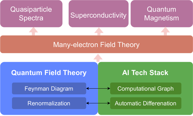
Figure 1: Overview of the ‘AI Tech Stack for QFT’ applied to many-electron field theory, illustrating its potential in advancing research across quasiparticle spectra, superconductivity, and quantum magnetism.

The paper is organized as follows: Section II details the computational graph representation of Feynman diagrams and the corresponding algorithms for constructing these graphs. Section III discusses the implementation of field-theoretic renormalization using the Taylor-mode AD algorithm. In Section IV, we introduce the Feynman diagram compiler, designed to implement these algorithms for quantum many-body field theory applications. Section V applies our algorithms to DiagMC calculations for the UEG. We conclude by summarizing our findings, discussing future work to enhance the ‘AI Tech Stack for QFT’ and exploring potential applications in Section VI.

II Feynman Diagrams as Computational Graphs

II.1 Feynman Diagrams

Feynman diagrams play an indispensable role in quantum many-body physics, serving as a graphical and computational method for understanding QFTs. These diagrams are particularly vital in scenarios where exact solutions are elusive and where interaction terms are small relative to kinetic terms. They provide a visual representation of the perturbative expansion of the action in powers of the interaction, linking fundamental interactions with physical observables in a clear and insightful manner.

In QFT, the action $S$ encapsulates the dynamics and interactions of particle fields. It can be formulated in various domains, such as momentum and imaginary time, or in alternative combinations like space-time, space-frequency, momentum-time, and momentum-frequency. This is represented as:

$$S=\int_{\mathbf{k}\tau}\bar{\psi}_{\mathbf{k}\tau}\hat{g}^{-1}_{\mathbf{k}\tau}\psi_{\mathbf{k}\tau}+\int_{\mathbf{k}\mathbf{k^{\prime}}\mathbf{q}\tau}V_{\mathbf{q}}\bar{\psi}_{\mathbf{k}+\mathbf{q}\tau}\bar{\psi}_{\mathbf{k^{\prime}}-\mathbf{q}\tau}\psi_{\mathbf{k^{\prime}}\tau}\psi_{\mathbf{k}\tau}.$$ (1)

Here, the integration measures imply integration over internal momenta $\mathbf{k}$, $\mathbf{k^{\prime}}$, and $\mathbf{q}$ and imaginary time $\tau$, while $\bar{\psi}$ and $\psi$ are either bosonic or fermionic Grassmann fields. The bare propagator of the particle is given by

$$\hat{g}_{\mathbf{k}\tau}^{-1}=\frac{\partial}{\partial\tau}+\epsilon_{\mathbf{k}}\quad\leftrightarrow\quad\hat{g}_{\mathbf{k}\omega_{n}}^{-1}=-i\omega_{n}+\epsilon_{\mathbf{k}},$$ (2)

where $\epsilon_{\mathbf{k}}$ is the energy dispersion. We will assume that the interaction potential $V_{\mathbf{q}}$ only depends on the momentum transfer $\mathbf{q}$, as for the Coulomb interaction between electrons. The discussions and methodologies in this paper can be generalized to encompass more complex, nonlocal, and dynamical interactions.

The perturbative treatment in QFT allows Feynman diagrams to depict correlation and vertex functions as power series expansions of the interaction. Each term in this series represents different particle interactions, graphically illustrated in the diagrams. In Feynman diagrams, the propagator $g_{\mathbf{k}\tau}$ and the interaction potential $V_{\mathbf{q}}$ are represented as edges, intersecting at vertices. A notable application is in computing the self-energy (see Fig. 2), a key concept in many-body physics that describes changes in a particle’s energy and lifetime due to particle interactions. Self-energy Feynman diagrams effectively bridge the gap between basic particle properties and their modified states in a many-body environment, showcasing the diagrams’ extensive utility in QFT scenarios.

In QFT, Feynman diagrams provide a versatile framework, adaptable across various domain combinations. By assigning momentum and frequency variables to edges and spatial and temporal variables to vertices, they offer effective tools in different analytical contexts. While the focus here is on momentum and imaginary-time domains, the methodologies are broadly applicable.

Traditionally, applications of Feynman diagrams within condensed matter physics and material science have focused on one-loop approximations. Two prominent examples of this methodology are the GW approximation [5, 45, 46] for electronic band structure calculations and the Eliashberg equations [6, 7] for the study of superconductivity. However, the feasibility of calculating high-order diagrammatic contributions has significantly increased with the advancement of numerical techniques. This progress has since allowed for more thorough investigations of interacting quantum systems [47, 48, 49, 50, 51]. Two notable methods in this direction are:

1. Diagrammatic Monte Carlo (DiagMC) [8, 9, 10, 11, 12, 13, 14, 15, 52] : This stochastic method is utilized for the numerical evaluation of high-order Feynman diagrams. It has successfully studied correlated fermions in systems like the UEG [13, 32, 31, 23], the unitary Fermi gas [15, 14, 53, 54], and the Hubbard model [10, 55, 33, 41, 42, 56, 43, 44, 57]. The method, while effective, faces challenges such as the sign problem in highly oscillatory integrals.

2. Tensor Crossing Interpolation (TCI) [16, 17, 18] : Offering an alternative to stochastic sampling, TCI uses tensor network techniques and has been applied with notable success to the quantum impurity model. This method employs tensor trains to represent the sum of all Feynman diagrams, thus simplifying the computation of high-dimensional integrals into a series of more manageable one-dimensional integrals and enhancing both the numerical precision and speed.

In $d$ spatial dimensions, the $n$th-order perturbation of the self-energy $\Sigma^{(n)}$ consists of Feynman diagrams with $n$ instantaneous interaction lines ($2n$ vertices), representing an $n(d+1)$-dimensional integration

$$\Sigma^{(n)}=\int d\mathcal{V}\sum_{t\in\mathcal{T}_{n}}\,W_{t}^{(n)}(\mathcal{V})$$ (3)

with measure $d\mathcal{V}=\prod^{n}_{i=1}d^{d}k_{i}d\tau_{i}$ and internal variables $\mathcal{V}=(\mathbf{k}_{1},\cdots,\mathbf{k}_{n};\tau_{1},\cdots,\tau_{n})$. Here the summation is over the set of all $n$th-order diagram topologies $\mathcal{T}_{n}$ (see Fig. 2) which, without the use of resummation techniques, grows as $\mathcal{O}(n!)$ [11]. Thus, the effectiveness of both DiagMC and TCI hinges on their efficiency in evaluating high-order Feynman diagrams, i.e., in computing the total weight function $\sum_{t\in\mathcal{T}_{n}}\,W_{t}^{(n)}(\mathcal{V})$ over many different internal variable configurations $\mathcal{V}$ throughout the simulation. This critical challenge leads into the next section, where we will explore a compact computational graph representation of Feynman diagrams.

Figure 2: Feynman diagrams in the bare expansion of the self-energy. The bare propagator $g$ and interaction $V$ are represented by directed and dashed lines, respectively. We use an abbreviated notation $1\equiv\tau_{1}$ to denote the indices of the imaginary time variables. We omit the momentum variables for simplicity.

II.2 Computational Graph Representation

Building on our review of Feynman diagrams in QFT, we now turn to their intriguing connection with computational graphs. This concept, more familiar in the realms of computer science and ML, provides a fresh perspective for managing the complexities involved in the numerical evaluation of high-order Feynman diagrams.

Computational graphs are structures composed of nodes and directed edges denoting mathematical operations and the flow of data or variables between these operations, respectively. This framework is adept at decomposing intricate calculations into a series of simpler, interconnected steps.

Applying this to Feynman diagrammatic integration (referenced in Eq.(3)), the weight function $\sum_{t\in\mathcal{T}_{n}}\,W_{t}^{(n)}(\mathcal{V})$ is interpretable as a computational graph. This graph’s structure includes propagators $g$ and interactions $V$ as initial nodes (‘leaves’), followed by a layer of multiplication nodes representing distinct Feynman diagrams, each combining a specific subset of leaves. The final layer is a summation operation that aggregates all multiplication nodes, culminating in the final integrand.

Figure 3: Illustration of the computational graph of two 4-point vertex function Feynman diagrams. These diagrams are distinguished by the exchange of interaction lines. The graph integrates both momentum (edge-dependent) and imaginary-time (vertex-dependent) variables. Factorization of shared propagators and interactions results in a compact computational graph, characterized by elementary operations such as addition, multiplication, and power operations.

Optimizing the computational graph for Feynman diagrams is essential for their integration in Quantum Field Theory (QFT). While recent advances have enhanced the efficiency of diagrams in the space-time representation, the momentum and frequency representations—which align more intrinsically with the fundamental principles of QFT—present a unique set of optimization challenges that are not yet fully explored. An initial attempt to address these challenges involved grouping Feynman diagrams into Hugenholz diagrams [13], leading to computational graphs with interaction lines organized into tree structures, thereby cutting the number of multiplication nodes from $\mathcal{O}(2^{N})$ to $\mathcal{O}(N\log N)$. However, this advancement represents just the tip of the iceberg. While it significantly optimizes the interaction lines or ’leaves’ of these graphs, common higher-order sub-diagrams are left unfactored and are thus ripe for optimization.

The path to developing a highly compressed computational graph for Feynman diagrams is marked by two major challenges. The first is the selection of internal variable configurations that maximize the overlap of common sub-diagrams between different Feynman diagrams. Given the vast number of internal variable configurations, only a carefully selected few result in the significant overlap essential for optimization. The second challenge involves efficiently identifying and extracting these overlapping sub-diagrams. Current methods like global common subexpression elimination (CSE) algorithms [58, 59], while promising in theory, face scalability issues, limiting their practicality as the graph’s complexity and size increase with higher perturbation orders. Therefore, the development of scalable, universal algorithms for optimizing computational graph representations in QFT, especially for momentum or frequency representations, becomes a critical need.

In the following section, we will introduce a bottom-up approach that addresses these pressing challenges. Unlike traditional methods that build Feynman diagrams piece by piece, this approach directly constructs a compact computational graph. Its key advantage lies in its ability to automatically prevent the duplication of common sub-diagrams, thereby optimizing the graph’s structure from the start. This methodology streamlines the optimization process and significantly reduces the computational complexity associated with large-scale Feynman diagrams.

II.3 Graph Construction Algorithms

II.3.1 Perturbative Dyson-Schwinger Equations

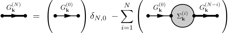
Figure 4: The $N$th-order Green’s function $G_{\mathbf{k}}^{(N)}$.

The Dyson-Schwinger equation (DSE), a bedrock within QFT, typically offers a non-perturbative lens to understand the interactions and propagations of particles by relating Green’s functions and vertex functions of varying particle numbers. However, in the context of our current exploration, we instead harness the power of the DSE to perturbatively generate compact computational graph representations for high-order Green’s function and vertex function Feynman diagrams.

We will illustrate the idea by showing how to generate a computational graph for the $N$th-order Green’s function from a given set of $N$th-order self-energy diagrams using the Dyson equation,

$$G^{(N)}_{\mathbf{k}}=G^{(0)}_{\mathbf{k}}\delta_{N,0}-G^{(0)}_{\mathbf{k}}\sum^{N}_{i=1}\Sigma^{(i)}_{\mathbf{k}}G^{(N-i)}_{\mathbf{k}}.$$ (4)

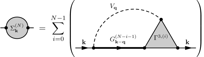
Figure 5: The $N$th-order self-energy $\Sigma_{\mathbf{k}}^{(N)}$.

To ensure clarity in our presentation, we have simplified the equations and figures to display only momentum labels. However, it is essential to understand that $N$-point vertex functions and Green’s functions can be represented as multi-dimensional tensors when we consider vertex-defined indices like imaginary-time and spin. For example, the Green’s function shown in Fig. 4, when including imaginary-time indices, transforms into a matrix form, expressed as $G_{\mathbf{q}}\rightarrow\left[G_{\mathbf{q}}\right]_{\tau_{i},\tau_{j}}$. In this tensorial representation, each node in the computational graph is a tensor, and operations such as multiplication are conducted through tensor contractions rather than simple scalar multiplication. This representation effectively turns Feynman diagrams into a tensor network, which opens up significant possibilities for computational optimization and efficiency.

The self-energy is related to the full (improper) 3-point vertex function by

$$\Sigma_{\mathbf{k}}^{(N)}=V_{\mathbf{q}}\sum^{N-1}_{i=0}G_{\mathbf{k}-\mathbf{q}}^{(N-i-1)}\Gamma^{3,(i)}_{\mathbf{k},\mathbf{k}-\mathbf{q};\mathbf{q}},$$ (5)

where the integration over internal momenta is implied. Similarly, the 3-point vertex function is related to the 4-point vertex function,

$$\Gamma^{3,(N)}_{\mathbf{k}_{1},\mathbf{k}_{2};\mathbf{q}}=\Gamma^{3,(0)}_{\mathbf{k}_{1},\mathbf{k}_{2};\mathbf{q}}\delta_{N,0}+\sum^{N-1}_{i=0}\Gamma^{4,(i)}_{\mathbf{k}_{1},\mathbf{k}_{2};\mathbf{p},\mathbf{p}+\mathbf{q}}\left[G_{\mathbf{p}+\mathbf{q}}G_{\mathbf{p}}\right]^{(N-i-1)},$$ (6)

where we define $\mathbf{q}\equiv\mathbf{k}_{1}-\mathbf{k}_{2}$ for brevity, and

$$\left[G_{\mathbf{p}+\mathbf{q}}G_{\mathbf{p}}\right]^{(N)}=\sum^{N}_{j=0}G^{(j)}_{\mathbf{p}+\mathbf{q}}G^{(N-j)}_{\mathbf{p}}$$ (7)

is the product of two Green’s functions truncated to total order $N$.

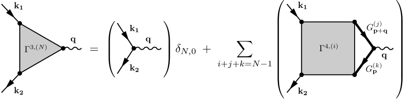
Figure 6: The $N$th-order three-point vertex $\Gamma^{3,(N)}_{\mathbf{k}_{1},\mathbf{k}_{2};\mathbf{q}}$.

Figure 7: The $N$th-order product of two Green’s functions $\left[G_{\mathbf{p}+\mathbf{q}}G_{\mathbf{p}}\right]^{(N)}$.

II.3.2 Perturbative Parquet Equations

The parquet equations [60, 61], integral to the study of quantum many-body physics, play a crucial role in detailing the interactions within complex systems, particularly in the analysis and construction of 4-point vertex functions. These equations intricately connect the full vertex functions to both their reducible and irreducible components across different interaction channels, thereby providing a detailed and comprehensive framework for understanding particle interactions.

The parquet equations are inherently iterative, designed to self-consistently solve for vertex functions [62, 63]. As in II.3.2, we will instead expand these equations perturbatively, so that each term in the parquet equations effectively corresponds to an equivalent diagrammatic structure. More specifically, the 4-point vertex function is built from a bottom-up approach using the parquet equations

$$\Gamma^{4,(N)}_{\mathbf{k}_{1},\mathbf{k}_{2};\mathbf{k}_{3},\mathbf{k}_{4}}=I^{(N)}_{\mathbf{k}_{1},\mathbf{k}_{2};\mathbf{k}_{3},\mathbf{k}_{4}}+\sum_{c\in\{ph,\overline{ph},pp\}}\Phi^{c,(N)}_{\mathbf{k}_{1},\mathbf{k}_{2};\mathbf{k}_{3},\mathbf{k}_{4}},$$ (8)

where $\mathbf{k}_{4}\equiv\mathbf{k}_{1}+\mathbf{k}_{2}-\mathbf{k}_{3}$, $I^{(N)}$ is the fully-irreducible 4-point vertex, and $\Phi^{c,(N)}$ and $\Gamma^{4,(N)}_{c}=\Gamma^{4,(N)}-\Phi^{c,(N)}$ are the 4-point reducible and irreducible vertices in channel $c\in\{ph,\overline{ph},pp\}$ evaluated to order $N$, respectively. The reducible vertices are defined by

$$\Phi^{ph,(N)}_{\mathbf{k}_{1},\mathbf{k}_{2};\mathbf{k}_{3},\mathbf{k}_{4}}=\sum_{i+j+k+l=N-1}\Gamma^{4,(i)}_{\mathbf{k}_{1},\mathbf{p}+\mathbf{k}_{3}-\mathbf{k}_{1};\mathbf{k}_{3},\mathbf{p}}\Gamma^{4,ph,(j)}_{\mathbf{p},\mathbf{k}_{2};\mathbf{p}+\mathbf{k}_{3}-\mathbf{k}_{1},\mathbf{k}_{4}}G^{(k)}_{\mathbf{p}}G^{(l)}_{\mathbf{p}+\mathbf{k}_{3}-\mathbf{k}_{1}},$$ (9)

$$\Phi^{\overline{ph},(N)}_{\mathbf{k}_{1},\mathbf{k}_{2};\mathbf{k}_{3},\mathbf{k}_{4}}=\zeta\sum_{i+j+k+l=N-1}\Gamma^{4,(i)}_{\mathbf{k}_{1},\mathbf{p}+\mathbf{k}_{2}-\mathbf{k}_{3};\mathbf{k}_{3},\mathbf{p}}\Gamma^{4,\overline{ph},(j)}_{\mathbf{p},\mathbf{k}_{2};\mathbf{p}+\mathbf{k}_{2}-\mathbf{k}_{3},\mathbf{k}_{4}}G^{(k)}_{\mathbf{p}}G^{(l)}_{\mathbf{p}+\mathbf{k}_{2}-\mathbf{k}_{3}},$$ (10)

$$\Phi^{pp,(N)}_{\mathbf{k}_{1},\mathbf{k}_{2};\mathbf{k}_{3},\mathbf{k}_{4}}=\frac{1}{2}\sum_{i+j+k+l=N-1}\Gamma^{4,(i)}_{\mathbf{k}_{1},\mathbf{k}_{2};\mathbf{p},\mathbf{k}_{1}+\mathbf{k}_{2}-\mathbf{p}}\Gamma^{4,pp,(j)}_{\mathbf{p},\mathbf{k}_{1}+\mathbf{k}_{2}-\mathbf{p};\mathbf{k}_{3},\mathbf{k}_{4}}G^{(k)}_{\mathbf{p}}G^{(l)}_{\mathbf{k}_{1}+\mathbf{k}_{2}-\mathbf{p}},$$ (11)

Figure 8: The $N$th-order four-point vertex minus fully-irreducible four-point vertex $\Gamma^{4,(N)}_{\mathbf{k}_{1},\mathbf{k}_{2};\mathbf{k}_{3},\mathbf{k}_{4}}-I^{(N)}_{\mathbf{k}_{1},\mathbf{k}_{2};\mathbf{k}_{3},\mathbf{k}_{4}}$.

where $\zeta=-1$ for fermions, and $+1$ for bosons, and are shown diagrammatically in Fig. 9.

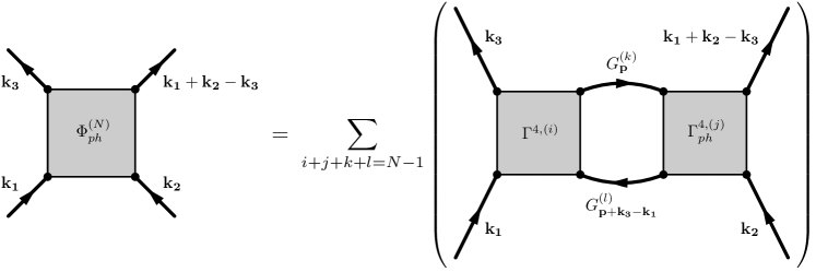
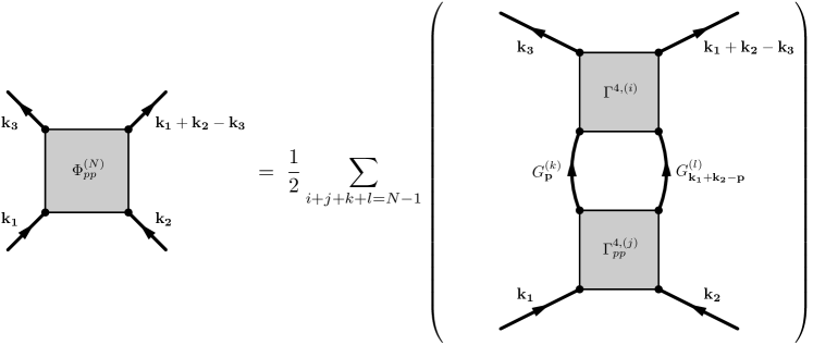
Figure 9: Diagrammatic construction of the $N$th-order reducible 4-point vertices $\Phi^{(N)}_{c}$ in each channel $c\in\{ph,\overline{ph},pp\}$ following Equations (9)–(11). Here $\zeta=-1$ for fermions, and $+1$ for bosons.

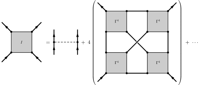
Figure 10: The fully-irreducible 4-point vertex $I$. The $N$th-order contribution is built bottom-up from the bare interaction $V$, Green’s function $G$ and reducible 4-point vertex $\Gamma^{4}$ in an analogous manner to Equations (9)–(11). This figure illustrates one specific permutation of external legs; however, the complete representation of $I$ includes all possible permutations, not depicted here for clarity.

The perturbative expansion of Eq.(8) leads to the formation of a computational graph as shown in Fig. 8. The intermediate nodes in this graph represent specific groups of 4-point vertex function sub-diagrams that share the same order and set of internal variables but differ in topology. The computational graph leverages these nodes to construct higher-order vertex function diagrams in a self-similar and hierarchical structure. This methodology allows for the reuse of intermediate nodes in constructing higher-order elements, thus eliminating redundant calculations and enhancing computational efficiency.

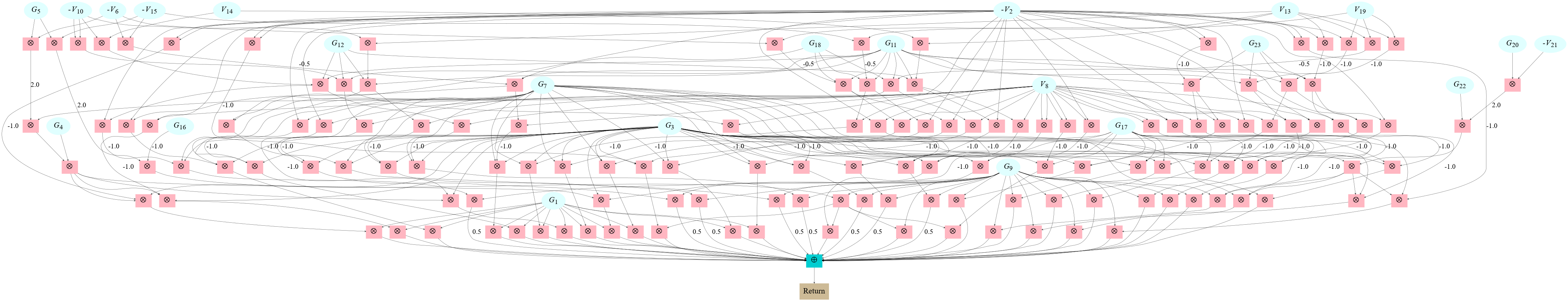
(a)

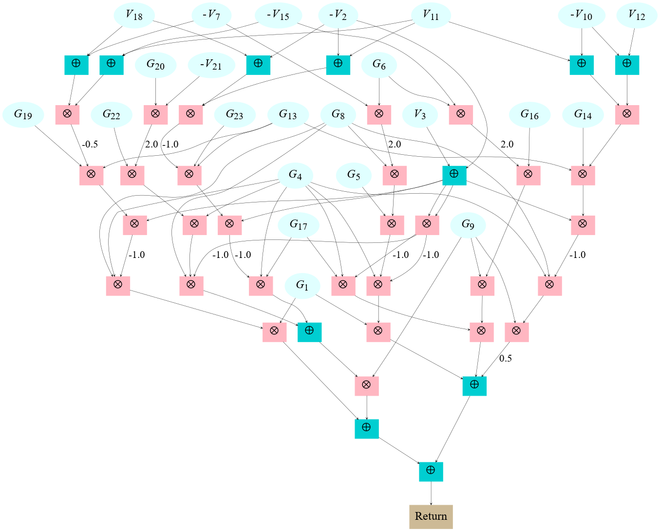
(b)

Figure 11: Computational graphs representing third-order Feynman diagrams for the dynamic self-energy of spinless fermions. (a) The naive approach graph aggregates Feynman diagrams, with each diagram being a product of propagators ‘G’ and interactions ‘V’. (b) The optimized graph, derived from parquet and Dyson-Schwinger equations, implements an efficient factorization of common sub-diagrams to reduce redundant calculations.

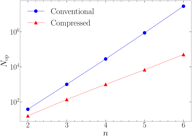
Figure 12: The total number of operations $N_{\rm op}$ required for calculating the $n$th-order self-energy, which is a measure of graph compactness. We compare $N_{\rm op}$ for a traditional summation of Feynman diagrams with the graph generated by Eqs.(5)–(11). The compressed graph is about three orders of magnitude more efficient than the conventional graph at the 6th order in perturbation theory.

Coupling the parquet equations with the DSE further extends the capability to generate compact computational graphs for not only 4-point vertex functions but also for 2- and 3-point vertex functions. This comprehensive approach significantly enriches the computational toolkit available in QFT, offering a practical and unified method for representing various vertex functions.

Implementing the above algorithms significantly compresses computational graphs. Figure 11 contrasts the third-order Feynman diagrams of the dynamic self-energy computational graph for spinless fermions before and after optimization using the parquet DSE (Eqs. (5)-(11)). The optimized graph exhibits marked compactness, enhancing computational efficiency. Further, quantitative benchmarking, detailed in Fig. 12, reveals that this optimized approach reduces the computational complexity of the 6th-order self-energy integrand by nearly three orders of magnitude compared to a conventional Feynman diagram computation.

III Renormalization as Automatic Differentiation

III.1 Field-theoretic Renormalization

Renormalization, a cornerstone in quantum field theory, plays a crucial role in unraveling the emergent properties of quantum many-body systems. Our primary objective in this section is to develop a compact computational representation of renormalized Feynman diagrams. To lay the foundation for this development, we first revisit the concept of renormalization, with an emphasis on its application in quantum many-body field theory.

Originally developed to address ultraviolet (UV) divergences in quantum electrodynamics (QED) [64], renormalization has evolved beyond its initial role as a mathematical regularization method. The introduction of the renormalization group approach by Wilson [65, 66] marked a paradigm shift, revealing how the characteristics of physical systems can vary across different energy scales. This perspective offered profound insights into scale-dependent behaviors in physics. Despite the conceptual advancements brought by Wilson’s approach, practical challenges persist in its computational application, especially for high-order calculations. This underlines the enduring importance of traditional field-theoretic renormalization methods [64], initially formulated for relativistic quantum field theories. Adapting these methods to non-relativistic quantum many-body field theories is a burgeoning area of research [67, 52, 68, 13, 21, 69], promising enhanced precision in calculations of complex many-body quantum phenomena.

Field-theoretical renormalization in perturbation theory involves redefining the starting point from bare parameters (defined at high-energy scales) to renormalized parameters that reflect low-energy dynamics. This shift aims to enhance the effectiveness of perturbation theory by aligning it more closely with the actual physical properties observed at lower energies. Consider, for example, renormalizing a bare propagator $\hat{g}$ into a quasiparticle propagator $\hat{G}$. This redefinition transforms the bare action into a renormalized action:

$$S\equiv S_{R}+S_{CT}$$ (12)

where

$$S_{R}=\int_{\mathbf{k}\tau}\bar{\psi}_{\mathbf{k}\tau}\hat{G}^{-1}_{\mathbf{k}\tau}\psi_{\mathbf{k}\tau}+\int_{\mathbf{k}\mathbf{k}^{\prime}\mathbf{q}\tau}V_{\mathbf{q}}\bar{\psi}_{\mathbf{k}+\mathbf{q}\tau}\bar{\psi}_{\mathbf{k}^{\prime}-\mathbf{q}\tau}\psi_{\mathbf{k}^{\prime}\tau}\psi_{\mathbf{k}\tau}.$$ (13)

The new diagrammatic series starts with zeroth-order terms generated from $S_{R}$ that already capture the correct low-energy physics. The higher-order terms involve counterterms generated from $S_{CT}$ that ensure the renormalized series reproduces the same physical result as the original series. The freedom of choosing $G$ and rearranging high-order terms provides numerous possible renormalization schemes, but most lead to badly diverging series. The field-theoretic renormalization addresses this challenge by offering a systematic way to generate diagrammatic series that are substantially more convergent, assuming that the renormalized action effectively captures the fundamental low-energy physics.

III.2 Constructive Renormalization Scheme

A field-theoretic renormalization scheme can be implemented in two ways: top-down or bottom-up. The top-down approach, commonly known as the BPHZ renormalization scheme, is a traditional method detailed in quantum field theory textbooks [1, 2, 3, 4]. It involves analyzing each Feynman diagram of the bare theory to identify and counteract the sub-diagrams that necessitate renormalization. Although effective, especially for UV divergent theories like QED [70, 71, 72, 73, 74], this approach can be computationally intensive. A recent development proposed in Ref. [21] takes the top-down renormalization scheme a step further by reorganizing the renormalized Feynman diagrams into determinants, which significantly reduces the associated computational complexity. However, it primarily operates in real space and time, limiting its adaptability for quantum field theories that are more conveniently expressed in the momentum representation.

In contrast, the bottom-up approach, which we will dub the “constructive renormalization scheme”, provides an alternative particularly well suited for quantum many-body problems where UV divergence is not a concern. While this approach has been utilized before, e.g., in solving the uniform electron gas problem in Ref. [13, 31], a systematic and explicit explanation of this technique remains limited. Here we provide a detailed explanation of this approach, focusing on its application in developing compact computational representations of renormalized Feynman diagrams. The algorithm entails three key steps:

1. Re-expansion of the Bare Propagator: The bare propagator is re-expanded into a power series of the renormalized propagator. This is driven by shifting one or more bare parameters to renormalized parameters defined at the low-energy limit. For instance, in the context of a Fermi liquid at zero temperature, the bare chemical potential $\mu$ is renormalized to the physically observed chemical potential $\mu_{R}=E_{\rm F}$, i.e., the Fermi energy. The bare propagator is then re-expanded as

   $$g(\mu)=G(\mu_{R})+\delta\mu\frac{\partial G(\mu_{R})}{\partial\mu_{R}}+\frac{\delta\mu^{2}}{2!}\frac{\partial^{2}G(\mu_{R})}{\partial\mu_{R}^{2}}+...$$ (14)

2. Construction of Renormalized Feynman Diagrams: The renormalized Feynman diagrams, as well as their counter-diagrams, are constructed from conventional Feynman rules using the re-expanded propagators. The diagrammatic series results in a double expansion in terms of both the interaction strength and the chemical potential shift. For instance, the shifted self-energy of the system can be organized in a double Taylor series,

   $$\Sigma(\xi,\delta\mu)=\sum_{n,m}\frac{\xi^{n}}{n!}\frac{\delta\mu^{m}}{m!}\Sigma^{(n,m)},$$ (15)

   where $\Sigma^{(n,m)}\equiv\frac{\partial^{m}\Sigma^{(n)}}{\partial\mu_{R}^{m}}$ is the self-energy contribution from diagrams with $n$ interaction lines and $m$ chemical potential counterterms. The variable $\xi=1$ is used to track the interaction order. Although each coefficient $\Sigma^{(n,m)}$ can be computed, the series still contains the unknown parameter $\delta\mu$, and thus cannot provide first-principles predictions.

3. Imposing Renormalization Conditions: The final step is to determine $\delta\mu$ by matching the theory with a measured quantity, known as the renormalization condition. Since the renormalized chemical potential $\mu_{R}$ is set as the physical Fermi energy, the chemical potential renormalization from the shifted self-energy should vanish at the Fermi surface (FS). This is implemented by expanding $\delta\mu$ as a power series of the interaction,

   $$\delta\mu=\sum_{i}\frac{\xi^{i}}{i!}\delta_{\mu}^{(i)},$$ (16)

   where $\delta_{\mu}^{(0)}=0$ since the shift is interaction-driven. The values of $\delta_{\mu}^{(i)}$ are derived by imposing the renormalization condition order-by-order:

   $$\left.\sum_{i=0}^{n}\frac{\delta_{\mu}^{(i)}}{i!}\Sigma^{(n,n-i)}\right|_{\rm FS}\equiv 0.$$ (17)

The success of this renormalization scheme hinges on the efficient computation of the Taylor coefficients $\Sigma^{(n,m)}$, which are essentially (functional) derivatives of the original self-energy Feynman diagrams. Note that in typical diagrammatic Monte Carlo calculations, the counterterm order $m$ can be as high as $n\sim 6$. As discussed previously, constructing a compact computational graph for the coefficients $\Sigma^{(n,0)}$ is straightforward. However, taking high-order derivatives for $m>0$ can lead to complexities. In the next subsection, we will discuss how to derive a compact representation that includes these high-order derivatives.

There exist alternative approaches to improving the convergence of perturbative series as proposed in Refs.[52, 69], which diverge slightly from the traditional field-theoretical renormalization scheme. While these methods share the common goal of enhancing series’ convergence, they differentiate themselves through the special renormalization conditions they employ. This variation in approach can result in power series exhibiting unique mathematical characteristics, a topic explored in depth in Ref.[52]. It is worth noting that the numerical techniques we develop in the subsequent subsection are also adaptable to these approaches.

Table 1: Examples of diagrams entering Eq.(15) grouped by number of interaction lines $n$ and chemical potential counterterm order $m$. The renormalized propagator $G(\mu_{R})$ and bare interaction $V$ are represented by directed and dashed lines, respectively, and the Green’s function counterterms $\delta^{(n)}_{g}$ are defined in Eq.(23).

III.3 Taylor-Mode Automatic Differentiation

In this work, we introduce an approach for computing renormalized Feynman diagrams in quantum many-body field theory, leveraging a compact computational graph representation. This methodology advances beyond the simpler computational graphs employed in previous studies for the uniform electron gas problem [13, 31]. It supports a more complex graph structure comprised of composite functions and a wide array of operators, which becomes particularly relevant in dealing with sophisticated operators emerging from the renormalization of nonlocal interactions [75].

A cornerstone of our approach is the use of Taylor-mode automatic differentiation (AD) [76, 77]. Unlike symbolic or numerical differentiation, which respectively rely on manipulating mathematical expressions or approximating derivatives at discrete points, AD computes derivatives precisely and efficiently [27]. It achieves this by breaking down functions into elementary operations and applying the chain rule in a systematic manner. This process results in exact derivative values, avoiding the drawbacks of symbolic manipulation’s complexity and the potential inaccuracies of numerical approximation. Taylor-mode AD, integral to our study, employs the classical Faà di Bruno’s formula and truncated Taylor series for calculating high-order derivatives. Originally developed in the ML community, this variant of AD is particularly well-suited to the rigorous demands of renormalized Feynman diagrams, enabling systematic computation of high-order Taylor coefficients $\Sigma^{(n,m)}$, as elaborated in Equation (17).

Our adaptation of the Taylor-mode AD algorithm to the realm of renormalized Feynman diagrams is grounded in two main principles:

1. Truncated Taylor Series of Nodes: Each node in the computational graph, after renormalization, becomes a truncated Taylor series in the renormalization parameter $\mu_{R}$. For a given node $f(\mu_{R})$, this is represented as:

   $$f(\mu_{R})=\sum_{m=0}^{N-1}\frac{\delta\mu_{R}^{m}}{m!}f^{(m)}(\mu_{R})+\mathcal{O}(\delta\mu_{R}^{N}),$$ (18)

   where $f^{(m)}$ denotes a compact computational graph for the sub-diagrams with $m$ counterterms, and $N$ is bounded by the truncated diagrammatic order.

2. Composite Function Derivatives: When a node $f(\mu_{R})$ feeds into a higher-level node, say $g(f(\mu_{R}))$, forming a composite function, the $m$th-order derivative of $g(\mu_{R})$ is dictated by Faà di Bruno’s formula:

   $$g^{(m)}(\mu_{R})=\sum\frac{m!}{b_{1}!b_{2}!\cdots b_{m}!}g^{(k)}(f)\prod_{l=1}^{m}\left(\frac{f^{(l)}(\mu_{R})}{l!}\right)^{b_{l}},$$ (19)

   where the sum spans all solutions in nonnegative integers $b_{i}$ satisfying $b_{1}+2b_{2}+\cdots+mb_{m}=m$ and $k:=b_{1}+\cdots+b_{m}$.

Applying these equations to different operators defines universal chain rules that can be recursively applied to construct a compact computational graph for high-order derivatives. For simple arithmetic operators like addition and multiplication, the chain rules are straightforward. For more complex operators, the chain rules can be automatically generated by a systematic algorithm provided in Ref. [28].

Taylor-mode AD significantly outperforms the naive recursion of first-order AD by merging duplicated terms that differ only by their prefactors. Compared to the naive approach, the computational complexity of an $l$th-order differentiation is reduced from $\mathcal{O}\left(e^{l}\right)$ to $\mathcal{O}\big{(}e^{\sqrt{l}}\big{)}$. This efficiency gain is demonstrated in Fig. 13, where we compare the total number of operations in the computational graphs for the $l$th-order interaction counterterms of all 4th-order parquet diagrams generated using Taylor-mode and nested first-order AD.

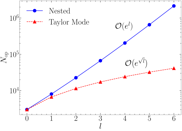
Figure 13: The total number of operations $N_{\rm op}$ in the $l$th-order interaction counterterms of all 4th-order $(n=4)$ parquet diagrams. The computational graphs for all counterterms are generated by differentiating $V(\lambda_{R})$ up to 6th order in $l$ (see Eq.(24)). Using nested first-order AD, $N_{\rm op}$ scales as $\mathcal{O}(e^{l})$ with $l$. For Taylor-mode AD, the scaling is reduced to $\mathcal{O}\big{(}e^{\sqrt{l}}\big{)}$.

IV AI Tech Stack for QFT

Figure 14: Architecture of the Feynman diagram compiler, delineating the transformation from diagrams to executable code. The compiler first translates Feynman diagrams into a unified computational graph, facilitating consistent treatment across various observables. Within this intermediate representation, local optimizations are applied to improve computational efficiency. Concurrently, automatic differentiation is employed to perform the renormalization scheme. The compiler back-end then generates optimized source code suitable for execution on diverse computational platforms, including CPUs and GPUs.

We introduce a methodology leveraging a compact computational graph representation for Feynman diagrams, combined with Taylor-mode AD for field-theoretic renormalization. A key insight from our research is the parallel between QFT constructs and AI techniques, facilitating the application of the AI tech stack to QFT numerical challenges.

Central to our approach is the use of computational graphs for evaluating Feynman diagrams, paralleling the structures used in ML architectures. Nodes in these graphs denote mathematical operations, while edges represent the flow of tensors. This structural similarity facilitates the incorporation of ML algorithms into QFT calculations, enhancing computational efficiency. Pathways of this interdisciplinary approach include adapting ML algorithms for QFT calculations, such as Taylor-mode AD for renormalization, and leveraging ML frameworks like JAX [29], TensorFlow [78], PyTorch [79], and Mindspore [80]. These frameworks provide optimized environments for processing computational graphs, efficiently utilizing diverse computing devices from CPUs and GPUs to emerging processor architectures.

To implement this concept, as illustrated in Fig. 14, we have developed a compiler architecture processing Feynman diagrams through a structured three-stage procedure, analogous to modern programming language compilers. This design significantly enhances the adaptability and computational efficiency of QFT calculations.

The ‘Front End’ of the compiler maps Feynman diagrams into a unified intermediate representation as a computational graph, ensuring consistent processing of various diagram types. The ‘Intermediate Representation’ stage optimizes and transforms a static computational graph. In contrast to the dynamic graphs used by some ML frameworks [79], a static graph representation enables deeper optimization and advanced rewriting protocol implementation. Notably, our application of Taylor-mode AD differs from existing methods that dynamically evaluate derivatives without constructing an explicit graph [26, 27, 28]. By utilizing a static graph, we facilitate more efficient AD processes, which is particularly advantageous for complex QFT calculations. In the ‘Back End’ phase, the compiler translates the optimized graph into executable code suitable for a range of computing platforms.

While the compiler itself is programmed in Julia, the ‘Back End’ architecture enables it to output source code in a range of other programming languages and machine learning frameworks, demonstrating its unique capability to bridge different computational ecosystems. Detailed implementation and user interface documentation are available in the open-source Julia package on GitHub: FeynmanDiagram.jl [81].

Although our computational graph primarily involves tensor operations, the current implementation translates these into scalar computations for CPU optimization. Nevertheless, we have observed significant performance gains with GPU parallelization. This improvement is clearly illustrated in Fig. 15, where we conduct a comparative analysis of evaluation times using the JAX framework on both CPU and GPU platforms. In the figure, $N_{\rm eval}$ denotes the number of batched evaluations of the computational graph. JAX’s vmap function plays a crucial role in this context, efficiently vectorizing operations across a batch of inputs for both hardware types. Our findings indicate that the vectorized JAX implementation consistently outperforms the serialized C language version. This advantage is likely attributable to JAX’s utilization of vector support features present in modern CPU architectures.

Future developments, such as incorporating tensor network optimizations [82, 83, 84, 85] for specialized hardware, could further enhance computational capabilities in QFT.

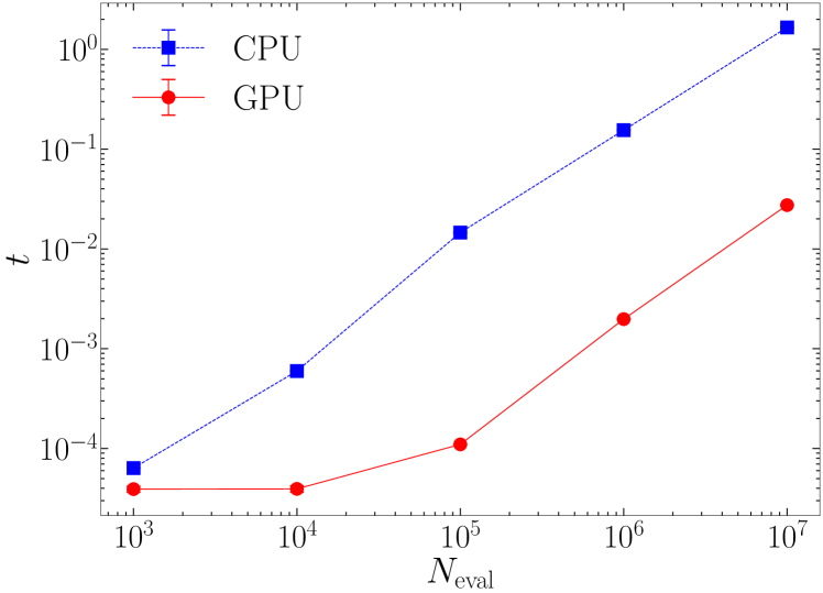
Figure 15: Comparison of computational graph evaluation times for the 4th-order self-energy using JAX on CPU (i7-11700, single-thread execution) and GPU (A100) platforms. The plot displays evaluation time ($t$) against the number of evaluations ($N_{eval}$) on a logarithmic scale. While the computational graph is primarily optimized for CPU, running JAX on the GPU accelerates computations by roughly two orders of magnitude over the CPU’s single-threaded implementation.

In discussing the application of machine learning to Feynman diagram computations, we note the recent work using PyTorch in Ref. [25]. While addressing a similar goal, our method differs by employing compression of computational graphs and Taylor-mode automatic differentiation, showcasing the diverse approaches and potential within this field.

V Application to the effective mass of the uniform electron gas

In this section, we deploy our algorithms and renormalization techniques, as elaborated in Sections II–III, to the calculation of the effective mass ratio $m^{*}/m$ in the uniform electron gas (UEG).

In the context of Landau Fermi liquid theory, the quasiparticle effective mass, denoted as $m^{*}/m$, is a key parameter that reflects the impact of electron-electron interactions on electron mobility [86, 87, 88, 89, 90]. The accurate determination of this ratio is crucial for a nuanced understanding of electron behavior in various materials.

Despite its importance, precisely calculating $m^{*}/m$ in the UEG presents substantial challenges due to constraints inherent in current computational techniques. Traditional diagrammatic perturbation theory, while widely used, faces two main limitations: (1) the results significantly vary depending on the renormalization scheme employed, and (2) it is often limited to low orders, thereby hindering a reliable estimation of systematic errors and validation of the outcomes [91]. Moreover, quantum Monte Carlo methods such as diffusion Monte Carlo (DMC) [92] and variational Monte Carlo (VMC) [93], though powerful, face their own challenges: they depend heavily on the choice of trial wave functions and are susceptible to finite-size effects, potentially distorting the results. These differing approaches yield not just varying but often contradictory results for the effective mass [32, 94, 95].

The resulting lack of methodological consensus for the effective mass behavior of the UEG underscores a critical gap in our ability to address nonlocal electron interactions in this model and highlights the need for more advanced and accurate computational techniques to resolve these issues.

V.1 Model and Methods

The UEG model represents interacting electrons in a uniform, inert, neutralizing background—it is the quintessential model of an electron liquid. Its simplicity and fundamental relevance make it a cornerstone in the study of electronic structures in materials science. The UEG provides a foundational framework for understanding electronic behavior in a broad spectrum of materials.

The bare action of the UEG is described by the following equation:

$$S_{0}= \int_{0}^{\beta}d\tau\Bigg{(}\sum_{\mathbf{k}\sigma}\bar{\psi}_{\mathbf{k}\sigma}(\partial_{\tau}+\epsilon_{k}-\mu)\psi_{\mathbf{k}\sigma}$$

$$+\frac{1}{2V}\sum_{\begin{subarray}{c}\mathbf{q}\neq 0\\ \mathbf{k}\mathbf{k^{\prime}}\sigma\sigma^{\prime}\end{subarray}}V_{q}\bar{\psi}_{\mathbf{k+q}\sigma}\bar{\psi}_{\mathbf{k^{\prime}-q}\sigma}\psi_{\mathbf{k^{\prime}}\sigma^{\prime}}\psi_{\mathbf{k}\sigma}\Bigg{)},$$ (20)

where $\psi$ and $\bar{\psi}$ are Grassmann fields, $\epsilon_{k}=\frac{\hbar^{2}k^{2}}{2m}$ is the kinetic energy term representing the UEG dispersion, and $V_{q}=\frac{4\pi e^{2}}{q^{2}}$ is the Coulomb interaction. Notably, the interaction strength inversely correlates with the electron density in the UEG model, so that an increase in density leads to weaker interactions. The density $\rho$ of the UEG is parameterized by the (dimensionless) Wigner-Seitz radius $r_{s}\equiv\bar{r}/a_{0}$, where $\bar{r}=(4\pi\rho/3)^{-1/3}$ is the average interparticle distance, and $a_{0}$ is the Bohr radius.

We now demonstrate how our method enables precise high-order perturbative calculations of the effective mass of the UEG. The central quantity in this problem is the momentum-frequency resolved self-energy $\Sigma(k,i\omega)$, and a number of quasiparticle properties can be readily extracted from it. The effective mass ratio $m^{*}/m$ is given by

$$\frac{m^{*}}{m}=Z^{-1}\cdot\left(1+\frac{m}{k_{\rm F}}\left.\frac{\partial\text{Re}\Sigma(k,0)}{\partial k}\right|_{k=k_{\rm F}}\right)^{-1},$$ (21)

where the renormalization constant

$$Z=\left(1-\left.\frac{\partial\text{Im}\Sigma(k_{\rm F},i\omega)}{\partial(i\omega)}\right|_{\omega=0}\right)^{-1}$$ (22)

gives the strength of the quasiparticle pole.

Our approach employs a diagrammatic method to calculate the self-energy. It should be noted that performing a bare expansion in terms of the Coulomb interaction leads to an unphysical divergence of the effective mass at the one-loop order, even in the weakly interacting limit. The introduction of a suitable renormalization scheme for a sound perturbative treatment of the UEG self-energy is thus essential. An effective and easily implementable scheme is proposed in Ref. [13]: conduct the perturbative expansion using a renormalized field theory describing electron interactions with an effective Yukawa potential. This theory involves two essential renormalizations: (1) adjusting the chemical potential to align with the physical Fermi energy, and (2) modifying the Coulomb interaction into a statically screened Yukawa interaction. This renormalization scheme has been successfully used to calculate various quasiparticle properties of the UEG, demonstrating its efficacy and reliability[32, 30, 23, 31].

Here, we provide a reformulation of this approach compatible with the Taylor-mode AD algorithm. Following the renormalization procedure outlined in Sec.III, we re-expand Eq.(20) in terms of a renormalized propagator $G(\mu_{R})$ and interaction $V(\lambda_{R})$, which are characterized by a renormalized chemical potential $\mu_{R}$ and static screening parameter $\lambda_{R}$, respectively, yielding the counterterms

$$g(\mu)-G({\mu_{R}}) =\sum^{\infty}_{n=1}\xi^{n}\frac{\delta\mu^{n}}{n!}\frac{\partial^{n}G(\mu_{R})}{\partial\mu^{n}_{R}}=\sum^{\infty}_{n=1}\xi^{n}\delta^{(n)}_{g},$$ (23)

$$V-V({\lambda_{R}}) =\sum^{\infty}_{n=1}\xi^{n}\frac{\delta\lambda^{n}}{n!}\frac{\partial^{n}V({\lambda_{R}})}{\partial\lambda^{n}_{R}}=\sum^{\infty}_{n=1}\xi^{n}\delta^{(n)}_{V}.$$ (24)

As discussed in Sec.III.2, the renormalized chemical potential is set to the physical Fermi energy $\mu_{R}=E_{\rm F}$. Here $V_{q}({\lambda})=\frac{4\pi e^{2}}{q^{2}+\lambda}$ is a Yukawa interaction with screening parameter $\lambda$—the bare interaction is recovered when $\lambda=0$. In contrast with the post-processing approach to $\delta\mu$, the free parameter $\delta\lambda=-\lambda_{R}$ is treated as a variational constant to optimize the convergence of the perturbative expansion.

In the present case, the self-energy is thus expanded as a Taylor series in three variables $\xi$, $\mu$, and $\lambda$,

$$\Sigma(\xi,\delta\mu,\delta\lambda)=\sum_{n,m,l}\frac{\xi^{n}}{n!}\frac{\delta\mu^{m}}{m!}\frac{\delta\lambda^{l}}{l!}\Sigma^{(n,m,l)},$$ (25)

where $\Sigma^{(n,m,l)}$ is the self-energy contribution from diagrams with $n$ interaction lines, $m$ chemical-potential counterterms, and $l$ interaction counterterms, and the variable $\xi=1$ is used to track the interaction order. The diagrams corresponding to $\Sigma^{(n,m,l)}$ are analogous to those listed in Tab. 1, but with the addition of $l$ interaction counterterms.

To evaluate the effective mass ratio, we first use Eq.(25) to express the frequency and momentum derivatives of the self-energy as power series in $\xi$,

$$\delta m(\xi,\delta\mu,\delta\lambda) =\sum^{\infty}_{n=0}\xi^{n}\delta m_{n}(\delta\mu,\delta\lambda),$$ (26)

where

$$\delta m_{n}(\delta\mu,\delta\lambda)=\sum_{m,l}\frac{\delta\mu^{m}}{m!}\frac{\delta\lambda^{l}}{l!}\frac{\delta m^{(n,m,l)}}{n!}$$ (27)

with analogous definitions for $\delta s(\xi,\delta\mu,\delta\lambda)$ and $\delta s_{n}(\delta\mu,\delta\lambda)$, and

$$\delta m^{(n,m,l)} =\frac{m}{k_{\rm F}}\left.\frac{\partial\text{Re}\Sigma^{(n,m,l)}(k,0)}{\partial k}\right|_{k=k_{\rm F}},$$ (28)

$$\delta s^{(n,m,l)} =\left.\frac{\partial\text{Im}\Sigma^{(n,m,l)}(k_{\rm F},i\omega)}{\partial(i\omega)}\right|_{\omega=0}.$$ (29)

Taylor-mode AD enables us to compute the momentum derivative in Eq.(28) on-the-fly such that the contributions $\delta m^{(n,m,l)}$ are simulated directly without introducing a discretization error. On the other hand, the frequency derivative in Eq.(29) must be estimated by finite difference methods due to the discrete nature of the Matsubara frequency axis at finite temperature $T$, so that $\partial\text{Im}\Sigma(k_{F},i\omega)/\partial(i\omega)=\lim_{T\rightarrow 0}\text{Im}\Sigma(k_{F},i\omega_{0})/\pi T$ [96].

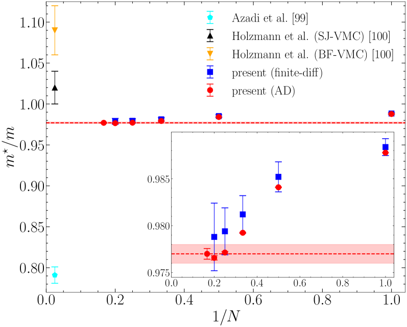
Figure 16: Effective mass ratio $m^{*}/m$ against perturbation order $N$ for 3D uniform electron gas at $r_{s}=5$ and $\lambda_{R}=1.125$. The tuning of $\lambda_{R}$ ensures optimal numerical convergence without altering the physical outcomes. The graph illustrates DiagMC results using Taylor-mode Automatic Differentiation (red circles) and finite differences (blue squares) for computing $\delta m^{(n,m,l)}$ coefficients (Eq.(28)), with both methods producing consistent data. Notably, our results are consistent with those from the recent Variational Quantum Monte Carlo (VMC) studies[95], but offer markedly smaller error bars, signifying a substantial improvement in precision. In contrast, there is a significant divergence from other Quantum Monte Carlo (QMC) results [94].

The computational graph methodology thus yields a simple and efficient procedure to compute the effective mass ratio of the UEG to order $N=n+m+l$ in the renormalized perturbation theory, which may be summarized as follows:

1. Construct computational graphs for the self-energy (see Fig. 11) and its high-order derivatives $\delta m^{(n,m,l)}$ and $\delta s^{(n,m,l)}$.

2. Perform a DiagMC integration using the constructed computational graphs. Here, we employ Markov-chain Monte Carlo (MCMC) to stochastically sample the integration variables, which include momenta and imaginary-time variables. To enhance the efficiency of the sampling process, we adopt an importance sampling technique. The variables are sampled following an adaptively learned distribution, known as the VEGAS map [97, 98], which optimizes the sampling process based on the distribution characteristics.

3. Carry out the renormalization post-processing procedure to compute the chemical potential shift $\delta\mu$ and the power series coefficients $\delta s_{n}(\delta\mu,\delta\lambda)$ and $\delta m_{n}(\delta\mu,\delta\lambda)$.

4. Compute the effective mass ratio $\frac{m^{*}}{m}=(1-\delta s)\cdot(1+\delta m)^{-1}$ from its power series expansion in $\xi$.

A notable advantage of this approach is that the computational graphs for the self-energy derivative contributions $\delta m^{(n,m,l)}$ and $\delta s^{(n,m,l)}$ may be pre-compiled once-and-for-all up to a given order $N$ and then reused for Monte Carlo simulations at, e.g., different values of the screening parameter $\lambda_{R}$ or temperature $T$.

In our method for calculating the self-energy and effective mass of the UEG, we introduce a comprehensive approach that includes a significantly greater number of Feynman diagrams compared to the approach used in Ref. [32]. This results in a more computationally demanding process, but it brings several distinct advantages. Unlike the previous method, which relies on dynamically screened Coulomb interactions parameterized in prior studies [32], our approach is not constrained by this parameterization. Consequently, we can extend our analysis to much lower temperatures, effectively approaching the zero-temperature limit, and probe beyond the previously established boundary of $r_{s}=4$. This broader and deeper exploration allows for a more accurate and thorough investigation of the UEG, free from the limitations and potential biases introduced by the reliance on pre-determined parameters.

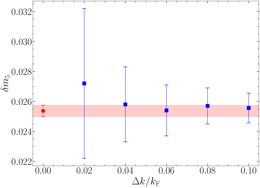
Figure 17: Demonstration of the advantages of AD over numerical finite differentiation in the 3D UEG with $r_{s}=5$ and $\lambda_{R}=1.125$. The red circle indicates the AD result for the momentum derivative of the 5th-order self-energy $\delta m_{5}$. The blue squares are the corresponding finite differences $\frac{m}{k_{\rm F}}\frac{\Delta\rm{Re}\Sigma^{(5)}(k,0)}{\Delta k}$ with $\Delta k/k_{\rm F}=k/k_{\rm F}-1=0.02,0.04,0.06,0.08$ and 0.1. Each data point is sampled for $10^{10}$ Monte Carlo steps.

V.2 Results

To demonstrate a concrete example of our computational graph methodology, we calculate the effective mass ratio $m^{*}/m$ for the 3D UEG with $r_{s}=5$ at effectively zero temperature.

Our computations yield a high-precision estimate of $m^{*}/m=0.977(1)$, as shown in Fig. 16. Near the optimal screening parameter, we find that the maximum perturbation order $N=6$ is already sufficient to estimate $m^{*}/m$ in the infinite-order limit. Our result demonstrates numerical convergence and a high degree of precision. Our finding is consistent with Holzmann’s quantum Monte Carlo (QMC) research [95], improving accuracy by two orders of magnitude, but differs from Azadi’s QMC studies [94]. This study notably demonstrates that the quasiparticle effective mass closely approximates the bare mass even in the correlated regime $r_{s}=5$, which is a remarkable result given the bare Coulomb repulsion is five times the strength of the bare kinetic energy and the quasiparticle weight is reduced to less than one half [99].

The AD technique plays a key role in enhancing the accuracy of our calculations, as shown in the inset of Fig. 16. Figure 17 shows that AD significantly improves the computational efficiency for the momentum derivative of the self-energy $\delta m$. Unlike the finite difference method, which suffers from large systematic (statistical) errors at wide (narrow) spacing $\Delta k$, AD provides a more robust and error-resistant approach. This improvement is crucial for our study, as the numerical precision of the self-energy derivatives $\delta m$ and $\delta s$ directly influences the reliability of the effective mass estimation.

For completeness, we mention that the DiagMC simulation with AD up to the maximum perturbation order $N=6$ shown in Fig. 16 requires roughly $10^{4}$ CPU (single-threaded process) hours. This computational demand, when compared to the resource-intensive nature of traditional methods, underscores the efficiency of our approach, especially considering the level of precision and reliability achieved in our results.

VI Conclusion and Perspective

In this paper, we have advanced techniques to address two fundamental challenges in QFT: the computation of Feynman diagrams and the implementation of renormalization. We introduced a compact computational graph representation for Feynman diagrams, developing generic algorithms to construct these representations for a wide range of physical observables. Furthermore, we implemented Taylor-mode AD atop this computational graph framework, efficiently realizing the field-theoretic renormalization scheme. Our algorithms significantly expedite the computation of renormalized Feynman diagrams, enhancing our capability to solve complex, nonlocal quantum many-body field theory problems.

A key insight from our work is the recognition of a parallel between fundamental elements in QFT and core AI technologies. The compact computational graphs and tensor operations central to Feynman diagram computations in QFT bear striking resemblances to architectures underpinning AI technologies. This parallelism opens an avenue for applying ML algorithms and techniques to QFT computations. Our utilization of Taylor-mode AD demonstrates the value of this interdisciplinary approach. Moreover, ML frameworks [78, 100, 79, 29, 80] provide optimized environments for managing computational graphs by making efficient use of specialized computing devices including CPUs, GPUs, and emerging processor architectures.

Implementing this concept, we developed a generic Feynman diagram compiler capable of translating diagrams of physical observables into efficient source code across various computing platforms. We combined this technique with a DiagMC algorithm to compute the effective mass of the three-dimensional UEG in the correlated regime. The resulting precision surpassed state-of-the-art quantum Monte Carlo simulations [95] by almost two orders of magnitude, underscoring the effectiveness of our computational graph representation and Taylor-mode AD.

We anticipate that similar techniques can be applied to first-principles calculations of other low-energy properties of the electron liquid, bridging fundamental QFT studies to ab initio calculations in material science. This includes computing various energy functionals required by Density Functional Theory (DFT) calculations [101, 102, 103, 104, 105] and determining the Coulomb pseudopotential urgently needed for ab initio predictions of the transition temperature in electron-phonon superconductors [106, 107, 36]. Additionally, our numerical framework has potential applications in studying fundamental quantum many-body models defined on lattices, such as the Hubbard model and frustrated spin systems.

Beyond physical problem-solving, our approach shows promise for calculating various forms of diagrammatic expansions, which is vital in addressing diverse many-body challenges. Recent advancements suggest the possibility of analytically integrating internal Matsubara frequency degrees of freedom to derive real-frequency linear response functions, thereby sidestepping the formidable numerical analytical continuation issues inherent in imaginary-time diagrammatic expansions [25]. Employing our compressed computational graph approach in this context may offer a more efficient means of computing dynamic response diagrams. Furthermore, the technique has potential applications in strong coupling expansions of theories with strong local interactions [43]. Here, the diagrammatic expansion involves many-body interactions that create complex Feynman diagram topologies and present significant computational challenges. Structuring these diagrams in a compressed computational graph format could be a fruitful direction for future exploration.

Looking forward, the ‘AI Tech Stack for QFT’ concept envisions a comprehensive framework that not only incorporates our efficient integrand computation strategy but also extends to emerging integration methods such as the normalizing flow techniques for high-dimensional integration [108, 109, 110, 111]. This combined approach has the potential to substantially improve the precision and speed of QFT calculations.

In the present implementation, we have optimized the computational graph primarily for CPU-based computations, where tensor operations are explicitly expanded into scalar operations. In future work, we plan to explore the integration of tensor network optimizations [82, 83, 84, 85]. This advancement could further enhance the efficiency of QFT computations, particularly when applied to specialized hardware.

In conclusion, this study takes a decisive step in harmonizing AI technology with QFT. The proposed ‘AI Tech Stack for QFT’ framework emerges as a tool with substantial potential in quantum physics research. It aims to not only streamline complex computational tasks , but also to offer fresh perspectives on correlated quantum systems. As this interdisciplinary field progresses, it is set to pave the way for novel discoveries and a deeper grasp of quantum interactions.

P.H., T.W., and D.C. contributed equally to this work.

References

- Bogoliubow and Parasiuk [1957] N. N. Bogoliubow and O. S. Parasiuk, On the multiplication of the causal function in the quantum theory of fields, Acta Mathematica 97, 227 (1957).
- Hepp [1966] K. Hepp, Proof of the bogoliubov-parasiuk theorem on renormalization, Communications in Mathematical Physics 2, 301 (1966).
- Zimmermann [1968] W. Zimmermann, The power counting theorem for minkowski metric, Communications in Mathematical Physics 11, 1 (1968).
- Zlmmbrmann [2000] W. Zlmmbrmann, Convergence of bogoliubov’s method of renormalization in momentum space, in Quantum Field Theory (Springer, 2000) pp. 217–243.
- Hedin [1965] L. Hedin, New method for calculating the one-particle green’s function with application to the electron-gas problem, Phys. Rev. 139, A796 (1965).
- Eliashberg [1960] G. Eliashberg, Interactions between electrons and lattice vibrations in a superconductor, Sov. Phys. JETP 11, 696 (1960).
- Eliashberg [1961] G. Eliashberg, Temperature green’s function for electrons in a superconductor, Sov. Phys. JETP 12, 1000 (1961).
- Prokof’ev and Svistunov [1998] N. V. Prokof’ev and B. V. Svistunov, Polaron problem by diagrammatic quantum monte carlo, Phys. Rev. Lett. 81, 2514 (1998).
- Prokof’ev and Svistunov [2008] N. Prokof’ev and B. Svistunov, Fermi-polaron problem: Diagrammatic monte carlo method for divergent sign-alternating series, Phys. Rev. B 77, 020408(R) (2008).
- Kozik et al. [2010] E. Kozik, K. V. Houcke, E. Gull, L. Pollet, N. Prokof’ev, B. Svistunov, and M. Troyer, Diagrammatic monte carlo for correlated fermions, Europhysics Letters 90, 10004 (2010).
- Rossi [2017] R. Rossi, Determinant diagrammatic monte carlo algorithm in the thermodynamic limit, Phys. Rev. Lett. 119, 045701 (2017).
- Prokof’ev and Svistunov [2007] N. Prokof’ev and B. Svistunov, Bold diagrammatic monte carlo technique: When the sign problem is welcome, Phys. Rev. Lett. 99, 250201 (2007).
- Chen and Haule [2019] K. Chen and K. Haule, A combined variational and diagrammatic quantum monte carlo approach to the many-electron problem, Nature communications 10, 1 (2019).
- Rossi et al. [2018a] R. Rossi, T. Ohgoe, K. Van Houcke, and F. Werner, Resummation of diagrammatic series with zero convergence radius for strongly correlated fermions, Phys. Rev. Lett. 121, 130405 (2018a).
- Van Houcke et al. [2012] K. Van Houcke, F. Werner, E. Kozik, N. V. Prokof’ev, B. V. Svistunov, M. Ku, A. Sommer, L. Cheuk, A. Schirotzek, and M. Zwierlein, Feynman diagrams versus fermi-gas feynman emulator, Nature Physics 8, 366 (2012).
- Oseledets [2011] I. V. Oseledets, Tensor-Train Decomposition, SIAM Journal on Scientific Computing 33, 2295 (2011).
- Dolgov and Savostyanov [2020] S. Dolgov and D. Savostyanov, Parallel cross interpolation for high-precision calculation of high-dimensional integrals, Computer Physics Communications 246, 106869 (2020).
- Núñez Fernández et al. [2022] Y. Núñez Fernández, M. Jeannin, P. T. Dumitrescu, T. Kloss, J. Kaye, O. Parcollet, and X. Waintal, Learning Feynman Diagrams with Tensor Trains, Phys. Rev. X 12, 041018 (2022).
- Moutenet et al. [2018] A. Moutenet, W. Wu, and M. Ferrero, Determinant monte carlo algorithms for dynamical quantities in fermionic systems, Phys. Rev. B 97, 085117 (2018).
- Šimkovic and Kozik [2019] F. Šimkovic and E. Kozik, Determinant monte carlo for irreducible feynman diagrams in the strongly correlated regime, Phys. Rev. B 100, 121102(R) (2019).
- Rossi et al. [2020] R. Rossi, F. Šimkovic, and M. Ferrero, Renormalized perturbation theory at large expansion orders, Europhysics Letters 132, 11001 (2020).
- Kozik [2023] E. Kozik, Combinatorial summation of Feynman diagrams: Equation of state of the 2D SU(N) Hubbard model (2023), arXiv:2309.13774 [cond-mat, physics:hep-th, physics:math-ph, physics:quant-ph].
- Hou et al. [2022] P.-C. Hou, B.-Z. Wang, K. Haule, Y. Deng, and K. Chen, Exchange-correlation effect in the charge response of a warm dense electron gas, Phys. Rev. B 106, L081126 (2022).
- Taheridehkordi et al. [2019] A. Taheridehkordi, S. H. Curnoe, and J. P. F. LeBlanc, Algorithmic Matsubara integration for Hubbard-like models, Phys. Rev. B 99, 035120 (2019).
- Burke and LeBlanc [2023] M. D. Burke and J. P. F. LeBlanc, TorchAmi: Generalized CPU/GPU Implementation of Algorithmic Matsubara Integration (2023), arXiv:2311.17189 [cond-mat, physics:hep-ph, physics:physics].
- Bettencourt et al. [2019] J. Bettencourt, M. J. Johnson, and D. Duvenaud, Taylor-mode automatic differentiation for higher-order derivatives in JAX, in Program Transformations for ML Workshop at NeurIPS 2019 (2019).
- Griewank and Walther [2008] A. Griewank and A. Walther, Evaluating derivatives: principles and techniques of algorithmic differentiation (SIAM, 2008).
- Tan [2023] S. Tan, Higher-Order Automatic Differentiation and Its Applications, Ph.D. thesis, Massachusetts Institute of Technology (2023).
- Bradbury et al. [2018] J. Bradbury, R. Frostig, P. Hawkins, M. J. Johnson, C. Leary, D. Maclaurin, G. Necula, A. Paszke, J. VanderPlas, S. Wanderman-Milne, and Q. Zhang, JAX: composable transformations of Python+NumPy programs (2018).
- Kukkonen and Chen [2021] C. A. Kukkonen and K. Chen, Quantitative electron-electron interaction using local field factors from quantum monte carlo calculations, Phys. Rev. B 104, 195142 (2021).
- LeBlanc et al. [2022] J. P. F. LeBlanc, K. Chen, K. Haule, N. V. Prokof’ev, and I. S. Tupitsyn, Dynamic response of an electron gas: Towards the exact exchange-correlation kernel, Phys. Rev. Lett. 129, 246401 (2022).
- Haule and Chen [2022] K. Haule and K. Chen, Single-particle excitations in the uniform electron gas by diagrammatic monte carlo, Scientific Reports 12, 2294 (2022).
- Deng et al. [2015] Y. Deng, E. Kozik, N. V. Prokof’ev, and B. V. Svistunov, Emergent bcs regime of the two-dimensional fermionic hubbard model: Ground-state phase diagram, Europhysics Letters 110, 57001 (2015).
- Šimkovic et al. [2021] F. Šimkovic, Y. Deng, and E. Kozik, Superfluid ground state phase diagram of the two-dimensional hubbard model in the emergent bardeen-cooper-schrieffer regime, Phys. Rev. B 104, L020507 (2021).
- Cai et al. [2022] X. Cai, T. Wang, N. V. Prokof’ev, B. V. Svistunov, and K. Chen, Superconductivity in the uniform electron gas: Irrelevance of the kohn-luttinger mechanism, Phys. Rev. B 106, L220502 (2022).
- Wang et al. [2023] T. Wang, X. Cai, K. Chen, B. V. Svistunov, and N. V. Prokof’ev, Origin of the coulomb pseudopotential, Phys. Rev. B 107, L140507 (2023).
- Hou et al. [2024] P. Hou, X. Cai, T. Wang, Y. Deng, N. V. Prokof’ev, B. V. Svistunov, and K. Chen, Precursory cooper flow in ultralow-temperature superconductors, Phys. Rev. Res. 6, 013099 (2024).
- Kulagin et al. [2013a] S. A. Kulagin, N. V. Prokof’ev, O. A. Starykh, B. V. Svistunov, and C. N. Varney, Bold diagrammatic monte carlo technique for frustrated spin systems, Phys. Rev. B 87, 024407 (2013a).
- Kulagin et al. [2013b] S. A. Kulagin, N. V. Prokof’ev, O. A. Starykh, B. V. Svistunov, and C. N. Varney, Bold diagrammatic monte carlo method applied to fermionized frustrated spins, Phys. Rev. Lett. 110, 070601 (2013b).
- Huang et al. [2016] Y. Huang, K. Chen, Y. Deng, N. V. Prokof’ev, and B. V. Svistunov, Spin-ice state of the quantum heisenberg antiferromagnet on the pyrochlore lattice, Phys. Rev. Lett. 116, 177203 (2016).
- Šimkovic et al. [2017] F. Šimkovic, Y. Deng, N. V. Prokof’ev, B. V. Svistunov, I. S. Tupitsyn, and E. Kozik, Magnetic correlations in the two-dimensional repulsive fermi-hubbard model, Phys. Rev. B 96, 081117(R) (2017).
- Kim et al. [2020] A. J. Kim, F. Šimkovic, and E. Kozik, Spin and charge correlations across the metal-to-insulator crossover in the half-filled 2d hubbard model, Phys. Rev. Lett. 124, 117602 (2020).
- Carlström [2021] J. Carlström, Strong-coupling diagrammatic monte carlo technique for correlated fermions and frustrated spins, Phys. Rev. B 103, 195147 (2021).
- Šimkovic et al. [2022] F. Šimkovic, R. Rossi, and M. Ferrero, Two-dimensional Hubbard model at finite temperature: Weak, strong, and long correlation regimes, Phys. Rev. Research 4, 043201 (2022).
- Godby et al. [1988] R. W. Godby, M. Schlüter, and L. J. Sham, Self-energy operators and exchange-correlation potentials in semiconductors, Phys. Rev. B 37, 10159 (1988).
- Hybertsen and Louie [1986] M. S. Hybertsen and S. G. Louie, Electron correlation in semiconductors and insulators: Band gaps and quasiparticle energies, Phys. Rev. B 34, 5390 (1986).
- Rohringer et al. [2018] G. Rohringer, H. Hafermann, A. Toschi, A. A. Katanin, A. E. Antipov, M. I. Katsnelson, A. I. Lichtenstein, A. N. Rubtsov, and K. Held, Diagrammatic routes to nonlocal correlations beyond dynamical mean field theory, Rev. Mod. Phys. 90, 025003 (2018).
- Kutepov [2016] A. L. Kutepov, Electronic structure of na, k, si, and lif from self-consistent solution of hedin’s equations including vertex corrections, Phys. Rev. B 94, 155101 (2016).
- Kutepov and Kotliar [2017] A. L. Kutepov and G. Kotliar, One-electron spectra and susceptibilities of the three-dimensional electron gas from self-consistent solutions of hedin’s equations, Phys. Rev. B 96, 035108 (2017).
- Wellenhofer et al. [2020] C. Wellenhofer, C. Drischler, and A. Schwenk, Dilute fermi gas at fourth order in effective field theory, Physics Letters B 802, 135247 (2020).
- Zerf et al. [2018] N. Zerf, P. Marquard, R. Boyack, and J. Maciejko, Critical behavior of the -gross-neveu-yukawa model at four loops, Phys. Rev. B 98, 165125 (2018).
- Rossi et al. [2016] R. Rossi, F. Werner, N. Prokof’ev, and B. Svistunov, Shifted-action expansion and applicability of dressed diagrammatic schemes, Phys. Rev. B 93, 161102(R) (2016).
- Rossi et al. [2018b] R. Rossi, T. Ohgoe, E. Kozik, N. Prokof’ev, B. Svistunov, K. Van Houcke, and F. Werner, Contact and momentum distribution of the unitary fermi gas, Phys. Rev. Lett. 121, 130406 (2018b).
- Van Houcke et al. [2019] K. Van Houcke, F. Werner, T. Ohgoe, N. V. Prokof’ev, and B. V. Svistunov, Diagrammatic monte carlo algorithm for the resonant fermi gas, Phys. Rev. B 99, 035140 (2019).
- Gukelberger et al. [2014] J. Gukelberger, E. Kozik, L. Pollet, N. Prokof’ev, M. Sigrist, B. Svistunov, and M. Troyer, -wave superfluidity by spin-nematic fermi surface deformation, Phys. Rev. Lett. 113, 195301 (2014).
- Šimkovic et al. [2020] F. Šimkovic, J. P. F. LeBlanc, A. J. Kim, Y. Deng, N. V. Prokof’ev, B. V. Svistunov, and E. Kozik, Extended Crossover from a Fermi Liquid to a Quasiantiferromagnet in the Half-Filled 2D Hubbard Model, Phys. Rev. Lett. 124, 017003 (2020).
- Lenihan et al. [2022] C. Lenihan, A. J. Kim, F. Šimkovic, and E. Kozik, Evaluating Second-Order Phase Transitions with Diagrammatic Monte Carlo: Néel Transition in the Doped Three-Dimensional Hubbard Model, Phys. Rev. Lett. 129, 107202 (2022).
- Cocke [1970] J. Cocke, Global common subexpression elimination, ACM SIGPLAN Notices 5, 20 (1970).
- Muchnick [1998] S. S. Muchnick, Advanced Compiler Design and Implementation (Morgan Kaufmann Publishers Inc., San Francisco, CA, USA, 1998).
- Li et al. [2016] G. Li, N. Wentzell, P. Pudleiner, P. Thunström, and K. Held, Efficient implementation of the parquet equations: Role of the reducible vertex function and its kernel approximation, Phys. Rev. B 93, 165103 (2016).
- Eckhardt et al. [2018] C. J. Eckhardt, G. A. H. Schober, J. Ehrlich, and C. Honerkamp, Truncated-unity parquet equations: Application to the repulsive hubbard model, Phys. Rev. B 98, 075143 (2018).
- Smith and Lande [1988] R. A. Smith and A. Lande, Parquet theory: The diagrams, in Condensed Matter Theories: Volume 3, edited by J. S. Arponen, R. F. Bishop, and M. Manninen (Springer US, Boston, MA, 1988) pp. 1–9.
- Kugler and von Delft [2018] F. B. Kugler and J. von Delft, Derivation of exact flow equations from the self-consistent parquet relations, New Journal of Physics 20, 123029 (2018).
- Dyson [1949] F. J. Dyson, The matrix in quantum electrodynamics, Phys. Rev. 75, 1736 (1949).
- Wilson and Kogut [1974] K. G. Wilson and J. Kogut, The renormalization group and the expansion, Physics Reports 12, 75 (1974).
- Wilson [1975] K. G. Wilson, The renormalization group: Critical phenomena and the kondo problem, Rev. Mod. Phys. 47, 773 (1975).
- Profumo et al. [2015] R. E. V. Profumo, C. Groth, L. Messio, O. Parcollet, and X. Waintal, Quantum Monte Carlo for correlated out-of-equilibrium nanoelectronic devices, Phys. Rev. B 91, 245154 (2015).
- Wu et al. [2017] W. Wu, M. Ferrero, A. Georges, and E. Kozik, Controlling Feynman diagrammatic expansions: Physical nature of the pseudogap in the two-dimensional Hubbard model, Phys. Rev. B 96, 041105(R) (2017).
- Kim et al. [2021] A. J. Kim, N. V. Prokof’ev, B. V. Svistunov, and E. Kozik, Homotopic action: A pathway to convergent diagrammatic theories, Phys. Rev. Lett. 126, 257001 (2021).
- Bethe [1947] H. A. Bethe, The electromagnetic shift of energy levels, Phys. Rev. 72, 339 (1947).
- Schwinger [1948] J. Schwinger, On quantum-electrodynamics and the magnetic moment of the electron, Phys. Rev. 73, 416 (1948).
- Feynman [1948] R. P. Feynman, Relativistic cut-off for quantum electrodynamics, Phys. Rev. 74, 1430 (1948).
- Aoyama et al. [2015] T. Aoyama, M. Hayakawa, T. Kinoshita, and M. Nio, Tenth-order electron anomalous magnetic moment: Contribution of diagrams without closed lepton loops, Phys. Rev. D 91, 033006 (2015).
- Hanneke et al. [2011] D. Hanneke, S. Fogwell Hoogerheide, and G. Gabrielse, Cavity control of a single-electron quantum cyclotron: Measuring the electron magnetic moment, Phys. Rev. A 83, 052122 (2011).
- Chen [2023] K. Chen, Systematic field-theoretic renormalization of non-local interactions (2023), manuscript in preparation.
- Engel et al. [2023] M. C. Engel, J. A. Smith, and M. P. Brenner, Optimal Control of Nonequilibrium Systems through Automatic Differentiation, Phys. Rev. X 13, 041032 (2023).
- Zhouyin et al. [2023] Z. Zhouyin, X. Chen, P. Zhang, J. Wang, and L. Wang, Automatic differentiable nonequilibrium Green’s function formalism: An end-to-end differentiable quantum transport simulator, Phys. Rev. B 108, 195143 (2023).
- Abadi et al. [2015] M. Abadi, A. Agarwal, P. Barham, E. Brevdo, Z. Chen, C. Citro, G. S. Corrado, A. Davis, J. Dean, M. Devin, S. Ghemawat, I. Goodfellow, A. Harp, G. Irving, M. Isard, Y. Jia, R. Jozefowicz, L. Kaiser, M. Kudlur, J. Levenberg, D. Mané, R. Monga, S. Moore, D. Murray, C. Olah, M. Schuster, J. Shlens, B. Steiner, I. Sutskever, K. Talwar, P. Tucker, V. Vanhoucke, V. Vasudevan, F. Viégas, O. Vinyals, P. Warden, M. Wattenberg, M. Wicke, Y. Yu, and X. Zheng, TensorFlow: Large-scale machine learning on heterogeneous systems (2015), software available from tensorflow.org.
- Paszke et al. [2019] A. Paszke, S. Gross, F. Massa, A. Lerer, J. Bradbury, G. Chanan, T. Killeen, Z. Lin, N. Gimelshein, L. Antiga, A. Desmaison, A. Kopf, E. Yang, Z. DeVito, M. Raison, A. Tejani, S. Chilamkurthy, B. Steiner, L. Fang, J. Bai, and S. Chintala, Pytorch: An imperative style, high-performance deep learning library, in Advances in Neural Information Processing Systems 32 (Curran Associates, Inc., 2019) pp. 8024–8035.
- min [2023] Huawei mindspore ai development framework, in Artificial Intelligence Technology (Springer Nature Singapore, Singapore, 2023) pp. 137–162.
- Fey [2024] https://github.com/numericalEFT/FeynmanDiagram.jl (2024), this is a link to the code of the Feynman diagram compiler in this paper.
- Tuovinen et al. [2019] R. Tuovinen, F. Covito, and M. A. Sentef, Efficient computation of the second-Born self-energy using tensor-contraction operations, The Journal of Chemical Physics 151, 174110 (2019).
- Shinaoka et al. [2020] H. Shinaoka, D. Geffroy, M. Wallerberger, J. Otsuki, K. Yoshimi, E. Gull, and J. Kuneš, Sparse sampling and tensor network representation of two-particle Green’s functions, SciPost Phys. 8, 012 (2020).
- Shinaoka et al. [2023] H. Shinaoka, M. Wallerberger, Y. Murakami, K. Nogaki, R. Sakurai, P. Werner, and A. Kauch, Multiscale space-time ansatz for correlation functions of quantum systems based on quantics tensor trains, Phys. Rev. X 13, 021015 (2023).
- Núñez Fernández et al. [2022] Y. Núñez Fernández, M. Jeannin, P. T. Dumitrescu, T. Kloss, J. Kaye, O. Parcollet, and X. Waintal, Learning feynman diagrams with tensor trains, Phys. Rev. X 12, 041018 (2022).
- Landau et al. [1987] L. Landau, E. Lifshitz, and L. Pitaevskij, Statistical physics, part 2: Theory of the condensed state, Course of theoretical physics 9 (1987).
- Silin [1958a] V. Silin, Theory of a degenerate electron liquid, Sov. Phys. JETP-USSR 6, 387 (1958a).
- Silin [1958b] V. Silin, On the theory of the anomalous skin effect in metals, Sov. Phys. JETP 6 (1958b).
- Nozières and Luttinger [1962] P. Nozières and J. M. Luttinger, Derivation of the landau theory of fermi liquids. i. formal preliminaries, Phys. Rev. 127, 1423 (1962).
- Luttinger and Nozières [1962] J. M. Luttinger and P. Nozières, Derivation of the landau theory of fermi liquids. ii. equilibrium properties and transport equation, Phys. Rev. 127, 1431 (1962).
- Yasuhara and Ousaka [1992] H. Yasuhara and Y. Ousaka, Effective mass, landau interaction function and self-energy of an electron liquid, International Journal of Modern Physics B 06, 3089 (1992).
- Ceperley and Alder [1980] D. M. Ceperley and B. J. Alder, Ground State of the Electron Gas by a Stochastic Method, Phys. Rev. Lett. 45, 566 (1980).
- Ceperley et al. [1977] D. Ceperley, G. V. Chester, and M. H. Kalos, Monte carlo simulation of a many-fermion study, Phys. Rev. B 16, 3081 (1977).
- Azadi et al. [2021] S. Azadi, N. D. Drummond, and W. M. C. Foulkes, Quasiparticle effective mass of the three-dimensional fermi liquid by quantum monte carlo, Phys. Rev. Lett. 127, 086401 (2021).
- Holzmann et al. [2023] M. Holzmann, F. Calcavecchia, D. M. Ceperley, and V. Olevano, Static self-energy and effective mass of the homogeneous electron gas from quantum monte carlo calculations, Phys. Rev. Lett. 131, 186501 (2023).
- Cerkoney et al. [2023] D. Cerkoney, P. Hou, Y. Deng, G. Kotliar, and K. Chen, Effective mass puzzle in the electron gas in two and three dimensions (2023), manuscript in preparation.
- Lepage [1978] G. P. Lepage, A new algorithm for adaptive multidimensional integration, Journal of Computational Physics 27, 192 (1978).
- Lepage [2021] G. P. Lepage, Adaptive multidimensional integration: vegas enhanced, Journal of Computational Physics 439, 110386 (2021).
- Holzmann et al. [2011] M. Holzmann, B. Bernu, C. Pierleoni, J. McMinis, D. M. Ceperley, V. Olevano, and L. Delle Site, Momentum Distribution of the Homogeneous Electron Gas, Phys. Rev. Lett. 107, 110402 (2011).
- Team et al. [2016] T. T. D. Team, R. Al-Rfou, G. Alain, A. Almahairi, C. Angermueller, D. Bahdanau, N. Ballas, F. Bastien, J. Bayer, A. Belikov, A. Belopolsky, Y. Bengio, A. Bergeron, J. Bergstra, V. Bisson, J. B. Snyder, N. Bouchard, N. Boulanger-Lewandowski, X. Bouthillier, A. de Brébisson, O. Breuleux, P.-L. Carrier, K. Cho, J. Chorowski, P. Christiano, T. Cooijmans, M.-A. Côté, M. Côté, A. Courville, Y. N. Dauphin, O. Delalleau, J. Demouth, G. Desjardins, S. Dieleman, L. Dinh, M. Ducoffe, V. Dumoulin, S. E. Kahou, D. Erhan, Z. Fan, O. Firat, M. Germain, X. Glorot, I. Goodfellow, M. Graham, C. Gulcehre, P. Hamel, I. Harlouchet, J.-P. Heng, B. Hidasi, S. Honari, A. Jain, S. Jean, K. Jia, M. Korobov, V. Kulkarni, A. Lamb, P. Lamblin, E. Larsen, C. Laurent, S. Lee, S. Lefrancois, S. Lemieux, N. Léonard, Z. Lin, J. A. Livezey, C. Lorenz, J. Lowin, Q. Ma, P.-A. Manzagol, O. Mastropietro, R. T. McGibbon, R. Memisevic, B. van Merriënboer, V. Michalski, M. Mirza, A. Orlandi, C. Pal, R. Pascanu, M. Pezeshki, C. Raffel, D. Renshaw, M. Rocklin, A. Romero, M. Roth, P. Sadowski, J. Salvatier, F. Savard, J. Schlüter, J. Schulman, G. Schwartz, I. V. Serban, D. Serdyuk, S. Shabanian, Étienne Simon, S. Spieckermann, S. R. Subramanyam, J. Sygnowski, J. Tanguay, G. van Tulder, J. Turian, S. Urban, P. Vincent, F. Visin, H. de Vries, D. Warde-Farley, D. J. Webb, M. Willson, K. Xu, L. Xue, L. Yao, S. Zhang, and Y. Zhang, Theano: A python framework for fast computation of mathematical expressions (2016), arXiv:1605.02688 [cs.SC] .
- Burke [2012] K. Burke, Perspective on density functional theory, The Journal of Chemical Physics 136, 150901 (2012).
- Jones [2015] R. O. Jones, Density functional theory: Its origins, rise to prominence, and future, Rev. Mod. Phys. 87, 897 (2015).
- Medvedev et al. [2017] M. G. Medvedev, I. S. Bushmarinov, J. Sun, J. P. Perdew, and K. A. Lyssenko, Density functional theory is straying from the path toward the exact functional, Science 355, 49 (2017).
- Mardirossian and Head-Gordon [2017] N. Mardirossian and M. Head-Gordon, Thirty years of density functional theory in computational chemistry: an overview and extensive assessment of 200 density functionals, Molecular Physics 115, 2315 (2017).
- Verma and Truhlar [2020] P. Verma and D. G. Truhlar, Status and challenges of density functional theory, Trends in Chemistry 2, 302 (2020), special Issue - Laying Groundwork for the Future.
- Margine and Giustino [2013] E. R. Margine and F. Giustino, Anisotropic Migdal-Eliashberg theory using Wannier functions, Phys. Rev. B 87, 024505 (2013).
- Poncé et al. [2016] S. Poncé, E. R. Margine, C. Verdi, and F. Giustino, EPW: Electron-phonon coupling, transport and superconducting properties using maximally localized Wannier functions, Computer Physics Communications 209, 116 (2016).
- Müller et al. [2019] T. Müller, B. Mcwilliams, F. Rousselle, M. Gross, and J. Novák, Neural Importance Sampling, ACM Transactions on Graphics 38, 1 (2019).
- Gao et al. [2020a] C. Gao, J. Isaacson, and C. Krause, i- flow : High-dimensional integration and sampling with normalizing flows, Machine Learning: Science and Technology 1, 045023 (2020a).
- Gao et al. [2020b] C. Gao, S. Höche, J. Isaacson, C. Krause, and H. Schulz, Event generation with normalizing flows, Phys. Rev. D 101, 076002 (2020b).
- Brady et al. [2021] J. Brady, P. Wen, and J. W. Holt, Normalizing flows for microscopic many-body calculations: An application to the nuclear equation of state, Phys. Rev. Lett. 127, 062701 (2021).