On the Communication Complexity of Approximate Pattern Matching

Abstract

The decades-old Pattern Matching with Edits problem, given a length-$n$ string $T$ (the text), a length-$m$ string $P$ (the pattern), and a positive integer $k$ (the threshold), asks to list all fragments of $T$ that are at edit distance at most $k$ from $P$. The one-way communication complexity of this problem is the minimum amount of space needed to encode the answer so that it can be retrieved without accessing the input strings $P$ and $T$.

The closely related Pattern Matching with Mismatches problem (defined in terms of the Hamming distance instead of the edit distance) is already well understood from the communication complexity perspective: Clifford, Kociumaka, and Porat [SODA 2019] proved that $\Omega(n/m\cdot k\log(m/k))$ bits are necessary and $\mathcal{O}(n/m\cdot k\log(m|\Sigma|/k))$ bits are sufficient; the upper bound allows encoding not only the occurrences of $P$ in $T$ with at most $k$ mismatches but also the substitutions needed to make each $k$-mismatch occurrence exact.

Despite recent improvements in the running time [Charalampopoulos, Kociumaka, and Wellnitz; FOCS 2020 and 2022], the communication complexity of Pattern Matching with Edits remained unexplored, with a lower bound of $\Omega(n/m\cdot k\log(m/k))$ bits and an upper bound of $\mathcal{O}(n/m\cdot k^{3}\log m)$ bits stemming from previous research. In this work, we prove an upper bound of $\mathcal{O}(n/m\cdot k\log^{2}m)$ bits, thus establishing the optimal communication complexity up to logarithmic factors. We also show that $\mathcal{O}(n/m\cdot k\log m\log(m|\Sigma|))$ bits allow encoding, for each $k$-error occurrence of $P$ in $T$, the shortest sequence of edits needed to make the occurrence exact. Our result further emphasizes the close relationship between Pattern Matching with Mismatches and Pattern Matching with Edits.

We leverage the techniques behind our new result on the communication complexity to obtain quantum algorithms for Pattern Matching with Edits: we demonstrate a quantum algorithm that uses $\mathcal{O}(n^{1+o(1)}/m\cdot\sqrt{km})$ queries and $\mathcal{O}(n^{1+o(1)}/m\cdot(\sqrt{k}m+k^{3.5}))$ quantum time. Moreover, when determining the existence of at least one occurrence, the algorithm uses $\mathcal{O}(\sqrt{n^{1+o(1)}/m}\cdot\sqrt{km})$ queries and $\mathcal{O}(\sqrt{n^{1+o(1)}/m}\cdot(\sqrt{k}m+k^{3.5}))$ time. For both cases, we establish corresponding lower bounds to demonstrate that the query complexity is optimal up to sub-polynomial factors.

1 Introduction

While a string is perhaps the most basic way to represent data, this fact makes algorithms working on strings more applicable and powerful. Arguably, the very first thing to do with any kind of data is to find patterns in it. The Pattern Matching problem for strings and its variations are thus perhaps among the most fundamental problems that Theoretical Computer Science has to offer.

In this paper, we study the practically relevant Pattern Matching with Edits variation [Sel80]. Given a text string $T$ of length $n$, a pattern string $P$ of length $m$, and a threshold $k$, the aim is to calculate the set $\mathrm{Occ}^{E}_{k}(P,T)$ consisting of (the starting positions of) all the fragments of $T$ that are at most $k$ edits away from the pattern $P$. In other words, we compute the set of $k$-error occurrences of $P$ in $T$, more formally defined as

$$\mathrm{Occ}^{E}_{k}(P,T)\coloneqq\{i\in\bm{[}\,0\,\bm{.\,.}\,n\,\bm{]}:\exists_{j\in\bm{[}\,i\,\bm{.\,.}\,n\,\bm{]}}\delta_{E}(P,T\bm{[}\,i\,\bm{.\,.}\,j\,\bm{)}\leq k)\},$$

where we utilize the classical edit distance $\delta_{E}$ (also referred to as the Levenshtein distance) [Lev65] as the distance measure. Here, an edit is either an insertion, a deletion, or a substitution of a single character.

Pattern Matching with Edits
Input: a pattern $P$ of length $m$, a text $T$ of length $n$, and an integer threshold $k>0$. Output: the set $\mathrm{Occ}^{E}_{k}(P,T)$.

Even though the Pattern Matching with Edits problem is almost as classical as it can get, with key algorithmic advances (from $\mathcal{O}(mn)$ time down to $\mathcal{O}(kn)$ time) dating back to the early and late 1980s [Sel80, LV88, LV89], major progress has been made very recently, when Charalampopoulos, Kociumaka, and Wellnitz [CKW22] obtained an $\tilde{\mathcal{O}}(n+k^{3.5}n/m)$-time solution and thereby broke through the 20-years-old barrier of the $\mathcal{O}(n+k^{4}n/m)$-time algorithm by Cole and Hariharan [CH02]. And the journey is far from over yet: the celebrated Orthogonal-Vectors-based lower bound for edit distance [BI18] rules out only $\mathcal{O}(n+k^{2-\Omega(1)}n/m)$-time algorithms (also consult [CKW22] for details), leaving open a wide area of uncharted algorithmic territory. In this paper, we provide tools and structural insights that—we believe—will aid the exploration of the said territory.

We add to the picture a powerful new finding that sheds new light on the solution structure of the Pattern Matching with Edits problem—similar structural results [BKW19, CKW20] form the backbone of the aforementioned breakthrough [CKW22]. Specifically, we investigate how much space is needed to store all $k$-error occurrences of $P$ in $T$. We know from [CKW20] that $\mathcal{O}(n/m\cdot k^{3}\log m)$ bits suffice since one may report the occurrences as $\mathcal{O}(k^{3})$ arithmetic progressions if $n=\mathcal{O}(m)$. However, such complexity is likely incompatible with algorithms running faster than $\tilde{\mathcal{O}}(n+k^{3}n/m)$. In this paper, we show that, indeed, $\mathcal{O}(n/m\cdot k\log^{2}m)$ bits suffice to represent the set $\mathrm{Occ}^{E}_{k}(P,T)$.

Formally, the communication complexity of Pattern Matching with Edits measures the space needed to encode the output so that it can be retrieved without accessing the input. We may interpret this setting as a two-party game: Alice is given an instance of the problem and constructs a message for Bob, who must be able to produce the output of the problem given Alice’s message. Since Bob does not have any input, it suffices to consider one-way single-round communication protocols.

mtheoremccompl The Pattern Matching with Edits problem admits a one-way deterministic communication protocol that sends $\mathcal{O}(n/m\cdot k\log^{2}m)$ bits. Within the same communication complexity, one can also encode the family of all fragments of $T\bm{[}\,i\,\bm{.\,.}\,j\,\bm{)}$ that satisfy $\delta_{E}(P,T\bm{[}\,i\,\bm{.\,.}\,j\,\bm{)})\leq k$, as well as all optimal alignments $P\leavevmode\hbox to16.67pt{\vbox to10.44pt{\text{[drawing]}}}T\bm{[}\,i\,\bm{.\,.}\,j\,\bm{)}$ for each of these fragments. Further, increasing the communication complexity to $\mathcal{O}(n/m\cdot k\log m\log(m|\Sigma|))$, where $\Sigma$ denotes the input alphabet, one can also retrieve the edit information for each optimal alignment.

Observe that our encoding scheme suffices to retrieve not only the set $\mathrm{Occ}^{E}_{k}(P,T)$ (which contains only starting positions of the $k$-error occurrences) but also the fragments of $T$ with edit distance at most $k$ from $P$. In other words, it allows retrieving all pairs $0\leq i\leq j\leq n$ such that $\delta_{E}(P,T\bm{[}\,i\,\bm{.\,.}\,j\,\bm{)})\leq k$.

We complement Section 1 with a simple lower bound that shows that our result is tight (essentially up to one logarithmic factor).

mtheoremcclb Fix integers $n,m,k$ such that $n/2\geq m>k>0$. Every communication protocol for the Pattern Matching with Edits problem uses $\Omega(n/m\cdot k\log(m/k))$ bits for $P=\mathtt{0}^{m}$ and some $T\in\{\mathtt{0},\mathtt{1}\}^{n}$.

Observe that our lower bound holds for the very simple case that the pattern is the all-zeros string and only the text contains nonzero characters. In this case, the edit distance of the pattern and another string depends only on the length and the number of nonzero characters in the other string, and we can thus easily compute the edit distance in linear time.

From Structural Insights to Better Algorithms: A Success Story

Let us take a step back and review how structural results aided the development of approximate-pattern-matching algorithms in the recent past.

First, let us review the key insight of [CKW20] that led to the breakthrough of [CKW22]. Crucially, the authors use that, for any pair of strings $P$ and $T$ with $|T|\leq{}^{3}{\mskip-3.5mu/\mskip-3.0mu}_{2}\,\cdot|P|$ and threshold $k\geq 1$, either (a) $P$ has at most $\mathcal{O}(k^{2})$ occurrences with at most $k$ edits in $T$, or (b) $P$ and the relevant part of $T$ are at edit distance $\mathcal{O}(k)$ to periodic strings with the same period. This insight helps as follows: First, one may derive that, indeed, all $k$-error occurrences of $P$ in $T$ form $\mathcal{O}(k^{3})$ arithmetic progressions. Second, it gives a blueprint for an algorithm: one has to tackle just two important cases: an easy nonperiodic case, where $P$ and $T$ are highly unstructured and $k$-error occurrences are rare, and a not-so-easy periodic case, where $P$ and $T$ are highly repetitive and occurrences are frequent but appear in a structured manner.

The structural insights of [CKW20] have found widespread other applications. For example, they readily yielded algorithms for differentially private approximate pattern matching [Ste24], approximate circular pattern matching problems [CKP⁺21, CKP⁺22, CPR⁺24], and they even played a key role in obtaining small-space algorithms for (online) language distance problems [BKS23], among others.

Interestingly, an insight similar to the one of [CKW20] was first obtained in [BKW19] for the much easier problem of Pattern Matching with Mismatches (where we allow neither insertions nor deletions) before being tightened and ported to Pattern Matching with Edits in [CKW20]. Similarly, in this paper, we port a known communication complexity bound from Pattern Matching with Mismatches to Pattern Matching with Edits; albeit with a much more involved proof. As proved in [CKP19], Pattern Matching with Mismatches problem admits a one-way deterministic $\mathcal{O}(k\log(m|\Sigma|/k))$-bit communication protocol. While we discuss later (in the Technical Overview) the result of [CKP19] as well as the challenges in porting it to Pattern Matching with Edits, let us highlight here that their result was crucial for obtaining an essentially optimal streaming algorithm for Pattern Matching with Mismatches.

Finally, let us discuss the future potential of our new structural results. First, as a natural generalization of [CKP19], $\hat{\mathcal{O}}(k)$-space algorithms for Pattern Matching with Edits should be plausible in the semi-streaming and (more ambitiously) streaming models, because $\hat{\mathcal{O}}(k)$-size edit distance sketches have been developed in parallel to this work [KS24]. Nevertheless, such results would also require $\hat{\mathcal{O}}(k)$-space algorithms constructing sketches and recovering the edit distance from the two sketches, and [KS24] does not provide such space-efficient algorithms. Second, our result sheds more light on the structure of the non-periodic case of [CKW20]: as it turns out, when relaxing the notion of periodicity even further, we obtain a periodic structure also for patterns with just a (sufficiently large) constant number of $k$-error occurrences. This opens up a perspective for classical Pattern Matching with Edits algorithms that are even faster than $\tilde{\mathcal{O}}(n/m+k^{3})$.

Application of our Main Result: Quantum Pattern Matching with Edits

As a fundamental problem, Pattern Matching with Edits has been studied in a plethora of settings, including the compressed setting [GS13, Tis14, BLR⁺15, CKW20], the dynamic setting [CKW20], and the streaming setting [Sta17, KPS21, BK23], among others. However, so far, the quantum setting remains vastly unexplored. While quantum algorithms have been developed for Exact Pattern Matching [HV03], Pattern Matching with Mismatches [JN23], Longest Common Factor (Substring) [GS23, AJ23, JN23], Lempel–Ziv factorization [GJKT24], as well as other fundamental string problems [AGS19, WY24, ABI⁺20, BEG⁺21, CKK⁺22], no quantum algorithm for Pattern Matching with Edits has been known so far. The challenge posed by Pattern Matching with Edits, in comparison to Pattern Matching with Mismatches, arises already from the fact that, while the computation of Hamming distance between two strings can be easily accelerated in the quantum setting, the same is not straightforward for the edit distance case. Only very recently, Gibney, Jin, Kociumaka, and Thankachan [GJKT24] demonstrated a quantum edit-distance algorithm with the optimal query complexity of $\tilde{\mathcal{O}}(\sqrt{kn})$ and the time complexity of $\tilde{\mathcal{O}}(\sqrt{kn}+k^{2})$.

We follow the long line of research on quantum algorithms on strings and employ our new structural results (combined with the structural results from [CKW20]) to obtain the following quantum algorithms for the Pattern Matching with Edits problem.

mtheoremqpmwe Let $P$ denote a pattern of length $m$, let $T$ denote a text of length $n$, and let $k>0$ denote an integer threshold.

1. There is a quantum algorithm that solves the Pattern Matching with Edits problem using $\hat{\mathcal{O}}(n/m\cdot\sqrt{km})$ queries and $\hat{\mathcal{O}}(n/m\cdot(\sqrt{k}m+k^{3.5}))$ time.

2. There is a quantum algorithm deciding whether $\mathrm{Occ}^{E}_{k}(P,T)\neq\varnothing$ using $\hat{\mathcal{O}}(\sqrt{n/m}\cdot\sqrt{km})$ queries and $\hat{\mathcal{O}}(\sqrt{n/m}\cdot(\sqrt{k}m+k^{3.5}))$ time.

Surprisingly, for $n=\mathcal{O}(m)$, we achieve the same query complexity as quantum algorithms for computing the (bounded) edit distance [GJKT24] and even the bounded Hamming distance of strings (a simple application of Grover search yields an $\tilde{\mathcal{O}}(\sqrt{kn})$ upper bound; a matching $\Omega(\sqrt{kn})$ lower bound is also known [BBC⁺01]). While we did not optimize the time complexity of our algorithms (reasonably, one could expect a time complexity of $\tilde{\mathcal{O}}(n/m\cdot(\sqrt{km}+k^{3.5}))$ based on our structural insights and [CKW22]), we show that our query complexity is essentially optimal by proving a matching lower bound.

mtheoremqpmwelb Let us fix integers $n\geq m>k>0$.

1. Every quantum algorithm that solves the Pattern Matching with Edits problem uses $\Omega(n/m\cdot\sqrt{k(m-k)})$ queries for $P=\mathtt{0}^{m}$ and some $T\in{\{\mathtt{0},\mathtt{1}\}}^{n}$.

2. Every quantum algorithm that decides whether $\mathrm{Occ}^{E}_{k}(P,T)\neq\varnothing$ uses $\Omega(\sqrt{n/m}\cdot\sqrt{k(m-k)})$ queries for $P=\mathtt{0}^{m}$ and some $T\in{\{\mathtt{0},\mathtt{1}\}}^{n}$.

Again, our lower bounds hold already for the case when the pattern is the all-zeroes string and just the text contains nonzero entries.

2 Technical Overview

In this section, we describe the technical contributions behind our positive results: Sections 1 and 1. We assume that $n\leq{}^{3}{\mskip-3.5mu/\mskip-3.0mu}_{2}\,m$ (if the text is longer, one may split the text into $\mathcal{O}(n/m)$ overlapping pieces of length $\mathcal{O}(m)$ each) and that $k=o(m)$ (for $k=\Theta(m)$, our results trivialize).

2.1 Communication Complexity of Pattern Matching with Mismatches

Before we tackle Section 1, it is instructive to learn how to prove an analogous result for Pattern Matching with Mismatches. Compared to the original approach of Clifford, Kociumaka, and Porat [CKP19], we neither optimize logarithmic factors nor provide an efficient decoding algorithm; this enables significant simplifications. Recall that our goal is to encode the set $\mathrm{Occ}^{H}_{k}(P,T)$, which is the Hamming-distance analog of the set $\mathrm{Occ}^{E}_{k}(P,T)$. Formally, we set

$$\mathrm{Occ}^{H}_{k}(P,T)\coloneqq\{i\in\bm{[}\,0\,\bm{.\,.}\,n-m\,\bm{]}:\delta_{H}(P,T\bm{[}\,i\,\bm{.\,.}\,i+m\,\bm{)})\leq k\}.$$

Without loss of generality, we assume that $\{0,n-m\}\subseteq\mathrm{Occ}^{H}_{k}(P,T)$, that is, $P$ has $k$-mismatch occurrences both as a prefix and as a suffix of $T$. Otherwise, either we have $\mathrm{Occ}^{H}_{k}(P,T)=\varnothing$ (which can be encoded trivially), or we can crop $T$ by removing the characters to the left of the leftmost $k$-mismatch occurrence and to the right of the rightmost $k$-mismatch occurrence.

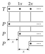
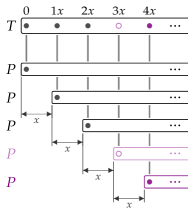
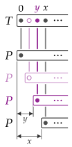
(a) The pattern $P$ occurs in $T$ starting at the positions $0$, $x$, and $2x$; these starting positions form the arithmetic progression $(ix)_{0\leq i\leq 2}$.	(b) Suppose that we were to identify an additional occurrence of $P$ in $T$ starting at position $4x$. Now, since occurrences start at $0,2x$, and $4x$ (which in particular implies that $T\bm{[}\,0\,\bm{.\,.}\,2x+|P|\,\bm{)}=T\bm{[}\,2x\,\bm{.\,.}\,4x+|P|\,\bm{)}$), as well as at position $x$, we directly obtain that there is also an occurrence that starts at position $3x$ in $T$; which means that the arithmetic progression from Figure 1(a) is extended to $(ix)_{0\leq i\leq 4}$. More generally, one may prove that any additional occurrence at a position $ix$ extends the existing arithmetic progression in a similar fashion.	(c) Suppose that we were to identify an additional occurrence of $P$ in $T$ starting at position $0<y<x$. Now, similarly to Figure 1(b), we can argue that there is also an occurrence that starts at every position of the form $i\text{gcd}(x,y)$ (this is a consequence of the famous Periodicity Lemma due to [FW65]; see Section 3)—again an arithmetic progression. Crucially, the difference of the arithmetic progression obtained in this fashion decreased by a factor of at least two compared to the initial arithmetic progression.

Figure 1: The structure of occurrences of exact pattern matching is easy: either all exact occurrences of $P$ in $T$ form an arithmetic progression or there is just one such occurrence (which we may also view as a degenerate arithmetic progression).
Depicted is a text $T$ and exact occurrences starting at the positions denoted above the text; we may assume that there is an occurrence that starts at position $0$ and that there is an occurrence that ends at position $|T|-1$.

Encoding All $k$-Mismatch Occurrences.

First, if $k=0$, as a famous consequence of the Periodicity Lemma [FW65], the set $\mathrm{Occ}^{H}_{0}(P,T)=\mathrm{Occ}(P,T)$ is guaranteed to form a single arithmetic progression (recall that $n\leq{}^{3}{\mskip-3.5mu/\mskip-3.0mu}_{2}\,m$ and see Lemma 3.1), and thus it can be encoded using $\mathcal{O}(\log m)$ bits. Consult Figure 1 for a visualization of an example.

If $k>0$, the set $\mathrm{Occ}^{H}_{k}(P,T)$ does not necessarily form an arithmetic progression. Still, we may consider the smallest arithmetic progression that contains $\mathrm{Occ}^{H}_{k}(P,T)$ as a subset. Since $0\in\mathrm{Occ}^{H}_{k}(P,T)$, the difference of this progression can be expressed as $g\coloneqq\gcd(\mathrm{Occ}^{H}_{k}(P,T))$.

A crucial property of the $\gcd(\cdot)$ function is that, as we add elements to a set maintaining its greatest common divisor $g$, each insertion either does not change $g$ (if the inserted element is already a multiple of $g$) or results in the value $g$ decreasing by a factor of at least $2$ (otherwise). Consequently, there is a set $\{0,n-m\}\subseteq S\subseteq\mathrm{Occ}^{H}_{k}(P,T)$ of size $|S|=\mathcal{O}(\log m)$ such that $\gcd(S)=\gcd(\mathrm{Occ}^{H}_{k}(P,T))=g$.

The encoding that Alice produces consists of the set $S$ with each $k$-mismatch occurrences $i\in S$ augmented with the mismatch information for $P$ and $T\bm{[}\,i\,\bm{.\,.}\,i+m\,\bm{)}$, that is, a set

$$\{(j,P[j],T[i+j]):j\in\bm{[}\,0\,\bm{.\,.}\,m\,\bm{)}\text{ such that }P[j]\neq T[i+j]\}.$$

For a single $k$-mismatch occurrence, the mismatch information can be encoded in $\mathcal{O}(k\log(m|\Sigma|))$ bits, where $\Sigma$ is the alphabet of $P$ and $T$. Due to $|S|=\mathcal{O}(\log m)$, the overall encoding size is $\mathcal{O}(k\log m\log(m|\Sigma|))$.

(a) Compare Figure 1(a). So far, we identified three occurrences of $P$ in $T$; each occurrence is an exact occurrence. Correspondingly, we have $S=\left\{(0,\varnothing),(x,\varnothing),(2x,\varnothing)\right\}$. With this set $S$, we obtain three different black components, which we depict with a circle, a diamond, or a star.	(b) The graph $\mathbf{G}_{S}$ that corresponds to Figure 2(a): observe how we collapsed the different patterns from Figure 2(a) into a single pattern $P$. In the example, we have three black components, that is, $\operatorname{bc}(\mathbf{G}_{S})=3$.
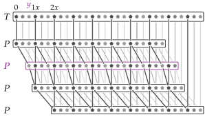
(c) Suppose that we were to identify an additional occurrence of $P$ in $T$ starting at position $0<y<x$ (highlighted in purple). From Figure 1(c), we know how the set of all occurrences changes, but—and this is the crucial point— we do not add all of these implicitly found occurrences to $S$, but just $y$. In our example, we observe that the black components collapse into a single black component, which we depict with a cloud.	(d) The graph $\mathbf{G}_{S}$ that corresponds to Figure 2(c): observe how we collapsed the different patterns from Figure 2(c) into a single pattern $P$. Highlighted in purple are some of the edges that we added due to the new occurrence that we added to $S$. In the example, we have one black components, that is, $\operatorname{bc}(\mathbf{G}_{S})=1$.
(e) Recovering an occurrence in $\mathbf{G}_{S}$ from Figure 2(d) that starts at position $\text{gcd}(x,y)$, illustrated for the first character of the pattern.

Figure 2: Compare Figure 1: we fully understand the easy structure of exact pattern matching. In this figure, we reinterpret our knowledge in terms of the encoding scheme of Alice for Pattern Matching with Mismatches (in particular we show just the occurrences included in the set $S$) and showcase how the corresponding graph $\mathbf{G}_{S}$ and its black components evolve.
We connect the same positions in $P$, as well as pairs of positions that are aligned by an occurrence of $P$ in $T$. As there are no mismatches, every such line implies that the connected characters are equal.
For each connected component of the resulting graph (a black component), we know that all involved positions in $P$ and $T$ must have the same symbol. For illustrative purposes, we assume that $x=3$ and we replace each character of a black component with a sentinel character (unique to that component), that is, we depict the strings $P^{\#}$ and $T^{\#}$.

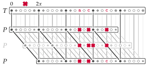
(a) Compare Figure 2(a). We depict mismatched characters in an alignment of $P$ to $T$ by placing a cross over the corresponding character in $P$. If we allow at most $3$ mismatches, we now do not have an occurrence starting at position $x$ anymore; hence we obtain six black components.	(b) The graph $\mathbf{G}_{S}$ that correspond to Figure 3(a). We make explicit characters that are different from the “default” character of a component; the corresponding red edges (that are highlighted) are exactly the mismatch information that is stored in $S$. For the remaining edges, the color depicts the color of the connected component that they belong to. In the example, we have four black components, that is, $\operatorname{bc}(\mathbf{G}_{S})=4$. (Observe that contrary to what the image might make you believe, not every “non-default” character needs to end in a highlighted red edge.)
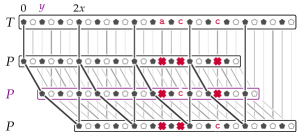
(c) Compare Figure 2(c). We are still able to identify an additional occurrence of $P$ in $T$ starting at position $0<y<x$ (highlighted in purple). Now, as before, connected components of $\mathbf{G}_{S}$ merge; this time, this also means that some characters that were previously part of a black component now become part of a red component (but crucially never vice-versa). In the example, this means that we now have just a single black component, that is, $\operatorname{bc}(\mathbf{G}_{S})=1$.	(d) The graph $\mathbf{G}_{S}$ for the situation in Figure 3(c). Again, we make explicit characters that are different from the “default” character of a component; the corresponding red edges (that are highlighted) are exactly the mismatch information that is stored in $S$. For the remaining edges, the color depicts the color of the connected component that they belong to (where purple highlights some of the black edges added due to the new occurrence).
(e) Checking for an occurrence at position $2\text{gcd}(x,y)$ (which would be an occurrence were it not for mismatched characters). We check two things, first that the black component aligns; and second, for the red component where we know all characters, we compute exactly the Hamming distance (which is $4$ in the example, meaning that there is no occurrence at the position in question).

Figure 3: Compared to Figure 2, we now have characters in $P$ and $T$ that mismatch. Again, we showcase how the corresponding graph $\mathbf{G}_{S}$ and its black components evolve; in the example, we allow for up to $k=3$ mismatches.
Again, for illustrative purposes, we assume that $x=3$ and we replace each character of a black component with a sentinel character (unique to that component), that is, we depict the strings $P^{\#}$ and $T^{\#}$.

Recovering the $k$-Mismatch Occurrences.

It remains to argue that the encoding is sufficient for Bob to recover $\mathrm{Occ}^{H}_{k}(P,T)$. To that end, consider a graph $\mathbf{G}_{S}$ whose vertices correspond to characters in $P$ and $T$. For every $i\in S$ and $j\in\bm{[}\,0\,\bm{.\,.}\,m\,\bm{)}$, the graph $\mathbf{G}_{S}$ contains an edge between $P[j]$ and $T[i+j]$. If $P[j]=T[i+j]$, then the edge is black; otherwise, the edge is red and annotated with the values $P[j]\neq T[i+j]$. Observe that Bob can reconstruct $\mathbf{G}_{S}$ using the set $S$ and the mismatch information for the $k$-mismatch occurrences at positions $i\in S$.

Next, we focus on the connected components of the graph $\mathbf{G}_{S}$. We say that a component is black if all of its edges are black and red if it contains at least one red edge. Observe that Bob can reconstruct the values of all characters in red components: the annotations already provide this information for vertices incident to red edges, and since black edges connect matching characters, the values can be propagated along black edges, ultimately covering all vertices in red components. The values of characters in black components remain unknown, but each black component is guaranteed to be uniform, meaning that every two characters in a single black component match.

The last crucial observation is that the connected components of $\mathbf{G}_{S}$ are very structured: for every remainder $c\in\bm{[}\,0\,\bm{.\,.}\,g\,\bm{)}$ modulo $g$, there is a connected component consisting of all vertices $P[i]$ and $T[i]$ with $i\equiv_{g}c$. This can be seen as a consequence of the Periodicity Lemma [FW65] applied to strings obtained from $P$ and $T$ by replacing each character with a unique identifier of its connected component. Consult Figure 2 for an illustration of an example for the special case if there are no mismatches and consult Figure 3 for a visualization of an example with mismatches.

Testing if an Occurrences Starts at a Given Position.

With these ingredients, we are now ready to explain how Bob tests whether a given position $i\in\bm{[}\,0\,\bm{.\,.}\,n-m\,\bm{]}$ belongs to $\mathrm{Occ}^{H}_{k}(P,T)$. If $i$ is not divisible by $g$, then for sure $i\notin\mathrm{Occ}^{H}_{k}(P,T)$. Otherwise, for every $j\in\bm{[}\,0\,\bm{.\,.}\,m\,\bm{)}$, the characters $P[j]$ and $T[i+j]$ belong to the same connected component. If this component is red, then Bob knows the values of $P[j]$ and $T[i+j]$, so he can simply check if the characters match. Otherwise, the component is black, meaning that $P[j]$ and $T[i+j]$ are guaranteed to match. As a result, Bob can compute the Hamming distance $\delta_{H}(P,T\bm{[}\,i\,\bm{.\,.}\,i+m\,\bm{)})$ and check if it does not exceed $k$. In either case (as long as $i$ is divisible by $g$), he can even retrieve the underlying mismatch information.

A convenient way of capturing Bob’s knowledge about $P$ and $T$ is to construct auxiliary strings $P^{\#}$ and $T^{\#}$ obtained from $P$ and $T$, respectively, by replacing all characters in each black component with a sentinel character (unique for the component). Then, $\mathrm{Occ}^{H}_{k}(P,T)=\mathrm{Occ}^{H}_{k}(P^{\#},T^{\#})$ and the mismatch information is preserved for the $k$-mismatch occurrences.

2.2 Communication Complexity of Pattern Matching with Edits

On a very high level, our encoding for Pattern Matching with Edits builds upon the approach for Pattern Matching with Mismatches presented above:

• Alice still constructs an appropriate size-$\mathcal{O}(\log m)$ set $S$ of $k$-error occurrences of $P$ in $T$, including a prefix and a suffix of $T$.

• Bob uses the edit information for the occurrences in $S$ to construct a graph $\mathbf{G}_{S}$ and strings $P^{\#}$ and $T^{\#}$, obtained from $P$ and $T$ by replacing characters in some components with sentinel characters so that $\mathrm{Occ}^{E}_{k}(P,T)=\mathrm{Occ}^{E}_{k}(P^{\#},T^{\#})$.

At the same time, the edit distance brings new challenges, so we also deviate from the original strategy:

• Connected components of $\mathbf{G}_{S}$ do not have a simple periodic structure, so $g=\gcd(S)$ loses its meaning. Nevertheless, we prove that black components still behave in a structured way, and thus the number of black components, denoted $\operatorname{bc}(\mathbf{G}_{S})$, can be used instead.

• The value $\operatorname{bc}(\mathbf{G}_{S})$ is not as easy to compute as $\gcd(S)$, so we grow the set $S\subseteq\mathrm{Occ}^{E}_{k}(P,T)$ iteratively. In each step, either we add a single $k$-error occurrence so that $\operatorname{bc}(\mathbf{G}_{S})$ decreases by a factor of at least $2$, or we realize that the information related to the alignments already included in $S$ suffices to retrieve all $k$-error occurrences of $P$ in $T$.

• Once this process terminates, there may unfortunately remain $k$-error occurrences whose addition to $S$ would decrease $\operatorname{bc}(\mathbf{G}_{S})$—yet, only very slightly. In other words, such $k$-error occurrences generally obey the structure of black components, but may occasionally violate it. We need to understand where the latter may happen and learn the characters behind the black components involved so that they are not masked out in $P^{\#}$ and $T^{\#}$. This is the most involved part of our construction, where we use recent insights relating edit distance to compressibility [CKW23, GJKT24] and store compressed representations of certain fragments of $T$.

2.2.1 General Setup

Technically, the set $S$ that Alice constructs contains, instead of $k$-error occurrences $T\bm{[}\,t\,\bm{.\,.}\,t^{\prime}\,\bm{)}$, specific alignments $P\leavevmode\hbox to16.67pt{\vbox to10.44pt{\text{[drawing]}}}T\bm{[}\,t\,\bm{.\,.}\,t^{\prime}\,\bm{)}$ of cost at most $k$. Every such alignment describes a sequence of (at most $k$) edits that transform $P$ onto $T\bm{[}\,t\,\bm{.\,.}\,t^{\prime}\,\bm{)}$; see Definition 3.3. In the message that Alice constructs, each alignment is augmented with edit information, which specifies the positions and values of the edited characters; see Definition 3.4. For a single alignment of cost $k$, this information takes $\mathcal{O}(k\log(m|\Sigma|))$ bits, where $\Sigma$ is the alphabet of $P$ and $T$.

Just like for Pattern Matching with Mismatches, we can assume without loss of generality that $P$ has $k$-error occurrences both as a prefix or as a suffix of $T$. Consequently, we always assume that $S$ contains an alignment $\mathcal{X}_{\mathsf{pref}}$ that aligns $P$ with a prefix of $T$ and an alignment $\mathcal{X}_{\mathsf{suf}}$ that aligns $P$ with a suffix of $T$.

The graph $\mathbf{G}_{S}$ is constructed similarly as for mismatches: the vertices are characters of $P$ and $T$, whereas the edges correspond to pairs of characters aligned by any alignment in $S$. Matched pairs of characters correspond to black edges, whereas substitutions correspond to red edges, annotated with the values of the mismatching characters. Insertions and deletions are also captured by red edges; see Definition 4.1 for details.

Again, we classify connected components of $\mathbf{G}_{S}$ into black (with black edges only) and red (with at least one red edge). Observe that Bob can reconstruct the graph $\mathbf{G}_{S}$ and the values of all characters in red components and that black components remain uniform, that is, every two characters in a single black component match. Consult Figure 4 for a visualization of an example.

Finally, we define $\operatorname{bc}(\mathbf{G}_{S})$ to be the number of black components in $\mathbf{G}_{S}$. If $\operatorname{bc}(\mathbf{G}_{S})=0$, then Bob can reconstruct the whole strings $P$ and $T$, so we henceforth assume $\operatorname{bc}(\mathbf{G}_{S})>0$.

First Insights into $\mathbf{G}_{S}$.

Our first notable insight is that black components exhibit periodic structure. To that end, write $P_{|S}$ for the subsequence of $P$ that contains all characters of $P$ that are contained in a black component in $\mathbf{G}_{S}$ and write $T_{|S}$ for the subsequence of $T$ that contains all characters of $T$ that are contained in a black component in $\mathbf{G}_{S}$. Then, for every $c\in\bm{[}\,0\,\bm{.\,.}\,\operatorname{bc}(\mathbf{G}_{S})\,\bm{)}$, there is a component consisting of all characters $P_{|S}[i]$ and $T_{|S}[i]$ such that $i\equiv_{\operatorname{bc}(\mathbf{G}_{S})}c$; for a formal statement and proof, consult Lemma 4.4. Also consult Figure 4(c) for an illustration of an example.

Next, we denote the positions in $P$ and $T$ of the subsequent characters of $P_{|S}$ and $T_{|S}$ belonging to a specific component $c\in\bm{[}\,0\,\bm{.\,.}\,\operatorname{bc}(\mathbf{G}_{S})\,\bm{)}$ as $\pi_{0}^{c},\pi_{1}^{c},\ldots$ and $\tau_{0}^{c},\tau_{1}^{c},\ldots$, respectively; see Definition 4.6. The characterization of the black components presented above implies that $\pi_{j}^{c}<\pi_{j^{\prime}}^{c^{\prime}}$ if and only if either $j<j^{\prime}$ or $j=j^{\prime}$ and $c<c^{\prime}$ (analogously for $\tau_{j}^{c}<\tau_{j^{\prime}}^{c^{\prime}}$). We assume that the $c$th black component contains $m_{c}$ characters of $P$ and $n_{c}$ characters in $T$; note that $m_{c}\in\{m_{0},m_{0}-1\}$ and $n_{c}\in\{n_{0},n_{0}-1\}$.

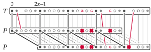
(a) Compare Figure 3(a). In addition to mismatched characters, we now also have missing characters in $P$ and $T$ (depicted by a white space). Further, as alignments for occurrences are no longer unique, we have to choose an alignment for each occurrence in the set $S$ (which can fortunately be stored efficiently).	(b) The graph $\mathbf{G}_{S}$ that corresponds to the situation in Figure 3(a). Observe that now, we also have a sentinel vertex $\bot$ to represent that an insertion or deletion happened. Observe further that due to insertions and deletions, the last empty star character of $T$ now belongs to the component of filled stars. In the example, we have two black components, that is, $\operatorname{bc}(\mathbf{G}_{S})=2$.
(c) An illustration of the additional notation that we use to analyze $\mathbf{G}_{S}$. Removing every character involved in a red component, we obtain the strings $T_{|S}$ and $P_{|S}$. For each black component, we number the corresponding characters in $P$ and $T$ from left to right.

Figure 4: Compare Figures 2 and 3. In addition to mismatches, we now also allow character insertions or deletions. In the example, we depict occurrence with at most $k=4$ edits.

2.2.2 Extra Information to Capture Close Alignments

By definition of the graph $\mathbf{G}_{S}$, the alignments in $S$ obey the structure of the black components. Specifically, for every $\mathcal{X}\in S$, there is a shift $i\in\bm{[}\,0\,\bm{.\,.}\,n_{0}-m_{0}\,\bm{]}$ such that $\mathcal{X}$ matches $P[\pi_{j}^{c}]$ with $T[\tau_{i+j}^{c}]$ for every $c\in\bm{[}\,0\,\bm{.\,.}\,\operatorname{bc}(\mathbf{G}_{S})\,\bm{)}$ and $j\in\bm{[}\,0\,\bm{.\,.}\,m_{c}\,\bm{)}$. The quasi-periodic structure of $P$ and $T$ suggests that we should expect further shifts $i\in\bm{[}\,0\,\bm{.\,.}\,n_{0}-m_{0}\,\bm{]}$ with low-cost alignments matching $P[\pi_{j}^{c}]$ with $T[\tau_{i+j}^{c}]$ for every $c\in\bm{[}\,0\,\bm{.\,.}\,\operatorname{bc}(\mathbf{G}_{S})\,\bm{)}$ and $j\in\bm{[}\,0\,\bm{.\,.}\,m_{c}\,\bm{)}$. Unfortunately, even if an optimum alignment $\mathcal{X}:P\leavevmode\hbox to16.67pt{\vbox to10.44pt{\text{[drawing]}}}T\bm{[}\,t\,\bm{.\,.}\,t^{\prime}\,\bm{)}$ matches $P[\pi_{j}^{c}]$ with $T[\tau_{i+j}^{c}]$, there is no guarantee that it also matches $P[\pi_{j^{\prime}}^{c^{\prime}}]$ with $T[\tau_{i+j^{\prime}}^{c^{\prime}}]$ for other values $c^{\prime}\in\bm{[}\,0\,\bm{.\,.}\,\operatorname{bc}(\mathbf{G}_{S})\,\bm{)}$ and $j^{\prime}\in\bm{[}\,0\,\bm{.\,.}\,m_{c^{\prime}}\,\bm{)}$. Even worse, it is possible that no optimal alignment $P\bm{[}\,\pi_{j}^{c-1}\,\bm{.\,.}\,\pi_{j}^{c+1}\,\bm{)}\leavevmode\hbox to16.67pt{\vbox to10.44pt{\text{[drawing]}}}T\bm{[}\,\tau_{i+j}^{c-1}\,\bm{.\,.}\,\tau_{i+j}^{c+1}\,\bm{)}$ matches $P[\pi_{j}^{c}]$ with $T[\tau_{i+j}^{c}]$. The reason behind this phenomenon is that the composition of optimal edit-distance alignments is not necessarily optimal (more generally, the edit information of optimal alignments $X\leavevmode\hbox to16.67pt{\vbox to10.44pt{\text{[drawing]}}}Y$ and $Y\leavevmode\hbox to16.67pt{\vbox to10.44pt{\text{[drawing]}}}Z$ is insufficient to recover $\delta_{E}(X,Z)$).

In these circumstances, our workaround is to identify a set $C_{S}\subseteq\bm{[}\,0\,\bm{.\,.}\,\operatorname{bc}(\mathbf{G}_{S})\,\bm{)}$ such that the underlying characters can be encoded in $\tilde{\mathcal{O}}(k|S|)$ space and every alignment $\mathcal{X}:P\leavevmode\hbox to16.67pt{\vbox to10.44pt{\text{[drawing]}}}T\bm{[}\,t\,\bm{.\,.}\,t^{\prime}\,\bm{)}$ that we need to capture matches $P[\pi_{j}^{c}]$ with $T[\tau_{i+j}^{c}]$ for every $c\in\bm{[}\,0\,\bm{.\,.}\,\operatorname{bc}(\mathbf{G}_{S})\,\bm{)}\setminus C_{S}$ and $j\in\bm{[}\,0\,\bm{.\,.}\,m_{c}\,\bm{)}$. For this, we investigate how an optimal alignment $\mathcal{X}:P\leavevmode\hbox to16.67pt{\vbox to10.44pt{\text{[drawing]}}}T\bm{[}\,t\,\bm{.\,.}\,t^{\prime}\,\bm{)}$ may differ from a canonical alignment $\mathcal{A}:P\leavevmode\hbox to16.67pt{\vbox to10.44pt{\text{[drawing]}}}T\bm{[}\,t\,\bm{.\,.}\,t^{\prime}\,\bm{)}$ that matches $P[\pi_{j}^{c}]$ with $T[\tau_{i+j}^{c}]$ for all $c\in\bm{[}\,0\,\bm{.\,.}\,\operatorname{bc}(\mathbf{G}_{S})\,\bm{)}$ and $j\in\bm{[}\,0\,\bm{.\,.}\,m_{c}\,\bm{)}$. Following recent insights from [CKW23, GJKT24] (see 3.7), we observe that the fragments of $P$ on which $\mathcal{A}$ and $\mathcal{X}$ are disjoint can be compressed into $\mathcal{O}(\delta_{E}^{\mathcal{A}}(P,T\bm{[}\,t\,\bm{.\,.}\,t^{\prime}\,\bm{)}))$ space (using Lempel–Ziv factorization [ZL77], for example). Moreover, the compressed size of each of these fragments is at most proportional to the cost of $\mathcal{A}$ on the fragment. Consequently, our goal is to understand where $\mathcal{A}$ makes edits and learn all the fragments of $P$ (and $T$) with a sufficiently high density of edits compared to the compressed size. Due to the quasi-periodic nature of $P$ and $T$, for each $c\in\bm{[}\,0\,\bm{.\,.}\,\operatorname{bc}(\mathbf{G}_{S})\,\bm{)}$, all characters in the $c$th black component are equal to $T[\tau_{0}^{c}]$, so we can focus on learning fragments of $T\bm{[}\,\tau_{0}^{0}\,\bm{.\,.}\,\tau_{0}^{\operatorname{bc}(\mathbf{G}_{S})-1}\,\bm{]}$.

The bulk of the alignment $\mathcal{A}$ can be decomposed into pieces that align $P\bm{[}\,\pi_{j}^{c}\,\bm{.\,.}\,\pi_{j}^{c+1}\,\bm{)}$ onto $T\bm{[}\,\tau_{i+j}^{c}\,\bm{.\,.}\,\tau_{i+j}^{c+1}\,\bm{)}$. In Lemma 4.9, we prove that $\delta_{E}(P\bm{[}\,\pi_{j}^{c}\,\bm{.\,.}\,\pi_{j}^{c+1}\,\bm{)},T\bm{[}\,\tau_{i+j}^{c}\,\bm{.\,.}\,\tau_{i+j}^{c+1}\,\bm{)})\leq\operatorname{w}_{S}(c)$, where $\operatorname{w}_{S}(c)$ is the total cost incurred by alignments in $S$ on all fragments $P\bm{[}\,\pi_{j^{\prime}}^{c}\,\bm{.\,.}\,\pi_{j^{\prime}}^{c+1}\,\bm{)}$ for $j^{\prime}\in\bm{[}\,0\,\bm{.\,.}\,m_{c}\,\bm{)}$. Intuitively, this is because the path from $P[\pi_{j}^{c}]$ to $T[\tau_{i+j}^{c}]$ in $\mathbf{G}_{S}$ allows obtaining an alignment $P\bm{[}\,\pi_{j}^{c}\,\bm{.\,.}\,\pi_{j}^{c+1}\,\bm{)}\leavevmode\hbox to16.67pt{\vbox to10.44pt{\text{[drawing]}}}T\bm{[}\,\tau_{i+j}^{c}\,\bm{.\,.}\,\tau_{i+j}^{c+1}\,\bm{)}$ as a composition of pieces of alignments in $S$ and their inverses. Every component $c\in\bm{[}\,0\,\bm{.\,.}\,\operatorname{bc}(\mathbf{G}_{S})\,\bm{)}$ uses distinct pieces, so the total weight $w:=\sum_{c}\operatorname{w}_{S}(c)$ does not exceed $k\cdot|S|$.

The weight function $\operatorname{w}_{S}(c)$ governs which characters of $T\bm{[}\,\tau_{0}^{0}\,\bm{.\,.}\,\tau_{0}^{\operatorname{bc}(\mathbf{G}_{S})-1}\,\bm{]}$ need to be learned. We formalize this with a notion of a period cover $C_{S}\subseteq\bm{[}\,0\,\bm{.\,.}\,\operatorname{bc}(\mathbf{G}_{S})\,\bm{)}$; see Definition 4.12. Most importantly, we require that $\bm{[}\,a\,\bm{.\,.}\,b\,\bm{]}\subseteq C_{S}$ holds whenever the compressed size of $T\bm{[}\,\tau_{0}^{a}\,\bm{.\,.}\,\tau_{0}^{b}\,\bm{]}$ is smaller than the total weight $\sum_{c=a-1}^{b}\operatorname{w}_{S}(c)$ (scaled up by an appropriate constant factor). Additionally, to handle corner cases, we also learn the longest prefix and the longest suffix of $T\bm{[}\,\tau_{0}^{0}\,\bm{.\,.}\,\tau_{0}^{\operatorname{bc}(\mathbf{G}_{S})-1}\,\bm{]}$ of compressed size $\mathcal{O}(w+k)$. As proved in Lemma 4.13, the set $\{(c,T[\tau_{0}^{c}]):c\in C_{S}\}$ can be encoded in $\mathcal{O}((w+k)\log(m|\Sigma|))=\mathcal{O}(k|S|\log(m|\Sigma|))$ bits on top of the graph $\mathbf{G}_{S}$ (which can be recovered from the edit information for alignments in $S$).

Following the aforementioned strategy of comparing the regions where $\mathcal{X}:P\leavevmode\hbox to16.67pt{\vbox to10.44pt{\text{[drawing]}}}T\bm{[}\,t\,\bm{.\,.}\,t^{\prime}\,\bm{)}$ is disjoint with the canonical alignment $\mathcal{A}:P\leavevmode\hbox to16.67pt{\vbox to10.44pt{\text{[drawing]}}}T\bm{[}\,t\,\bm{.\,.}\,t^{\prime}\,\bm{)}$, we prove the following result. Due to corner cases arising at the endpoints of $T\bm{[}\,t\,\bm{.\,.}\,t^{\prime}\,\bm{)}$ and between subsequent fragments $T\bm{[}\,\tau_{i+j}^{0}\,\bm{.\,.}\,\tau_{i+j}^{\operatorname{bc}(\mathbf{G}_{S})-1}\,\bm{]}$ and $T\bm{[}\,\tau_{i+j+1}^{0}\,\bm{.\,.}\,\tau_{i+j+1}^{\operatorname{bc}(\mathbf{G}_{S})-1}\,\bm{]}$, the proof is rather complicated.

propositionprpclose Let $\mathcal{X}:P\leavevmode\hbox to16.67pt{\vbox to10.44pt{\text{[drawing]}}}T\bm{[}\,t\,\bm{.\,.}\,t^{\prime}\,\bm{)}$ be an optimal alignment of $P$ onto a fragment $T\bm{[}\,t\,\bm{.\,.}\,t^{\prime}\,\bm{)}$ such that $\delta_{E}(P,T\bm{[}\,t\,\bm{.\,.}\,t^{\prime}\,\bm{)})\leq k$. If there exists $i\in\bm{[}\,0\,\bm{.\,.}\,n_{0}-m_{0}\,\bm{]}$ such that $|\tau_{i}^{0}-t-\pi_{0}^{0}|\leq w+3k$, then the following holds for every $c\in\bm{[}\,0\,\bm{.\,.}\,\operatorname{bc}(\mathbf{G}_{S})\,\bm{)}\setminus C_{S}$:

1. $\mathcal{X}$ aligns $P[\pi^{c}_{j}]$ to $T[\tau^{c}_{i+j}]$ for every $j\in\bm{[}\,0\,\bm{.\,.}\,m_{c}\,\bm{)}$, and

2. $\tau^{c}_{i^{\prime}}\notin\bm{[}\,t\,\bm{.\,.}\,t^{\prime}\,\bm{)}$ for every $i^{\prime}\in\bm{[}\,0\,\bm{.\,.}\,n_{c}\,\bm{)}\setminus\bm{[}\,i\,\bm{.\,.}\,i+m_{c}\,\bm{)}$.

2.2.3 Extending $S$ with Uncaptured Alignments

Section 2.2.2 indicates that $S$ captures all $k$-error occurrences $T\bm{[}\,t\,\bm{.\,.}\,t^{\prime}\,\bm{)}$ such that $|\tau_{i}^{0}-t-\pi_{0}^{0}|\leq w+3k$ holds for some $i\in\bm{[}\,0\,\bm{.\,.}\,n_{0}-m_{0}\,\bm{]}$. As long as $S$ does not capture some $k$-error occurrence $T\bm{[}\,t\,\bm{.\,.}\,t^{\prime}\,\bm{)}$, we add an underlying optimal alignment $\mathcal{X}:P\leavevmode\hbox to16.67pt{\vbox to10.44pt{\text{[drawing]}}}T\bm{[}\,t\,\bm{.\,.}\,t^{\prime}\,\bm{)}$ to the set $S$. In Lemma 4.27, we prove that $\operatorname{bc}(\mathbf{G}_{S\cup\{\mathcal{X}\}})\leq\operatorname{bc}(\mathbf{G}_{S})/2$ holds for such an alignment $\mathcal{X}$. For this, we first eliminate the possibility of $t+\pi_{0}^{0}\gg\tau_{n_{0}-m_{0}}^{0}$ (using $\mathcal{X}_{\mathsf{suf}}\in S$, which matches $P[\pi_{0}^{0}]$ with $T[\tau_{n_{0}-m_{0}}^{0}]$). If $|\tau_{i}^{0}-t-\pi_{0}^{0}|>w+3k$ holds for every $i\in\bm{[}\,0\,\bm{.\,.}\,n_{0}\,\bm{)}$, on the other hand, then there is no $c\in\bm{[}\,0\,\bm{.\,.}\,\operatorname{bc}(\mathbf{G}_{S})\,\bm{)}$ such that $P[\pi_{0}^{c}]$ can be matched with any character in the $c$th connected component. Consequently, each black component becomes red or gets merged with another black component, resulting in the claimed inequality $\operatorname{bc}(\mathbf{G}_{S\cup\{\mathcal{X}\}})\leq\operatorname{bc}(\mathbf{G}_{S})/2$.

By Lemma 4.27 and since $\operatorname{bc}(\mathbf{G}_{S})\leq m$ holds when we begin with $|S|=2$, the total size $|S|$ does not exceed $\mathcal{O}(\log m)$ before we either arrive at $\operatorname{bc}(\mathbf{G}_{S})=0$, in which case the whole input can be encoded in $\mathcal{O}(k|S|\log(m|\Sigma|))$ bits, or $S$ captures all $k$-error occurrences. In the latter case, the encoding consists of the edit information for all alignments in $S$, as well as the set $\{(c,T[\tau_{0}^{c}]):c\in C_{S}\}$ encoded using Lemma 4.13. Based on this encoding, we can construct strings $P^{\#}$ and $T^{\#}$ obtained from $P$ and $T$, respectively, by replacing with $\#_{c}$ every character in the $c$th connected component for every $c\in\bm{[}\,0\,\bm{.\,.}\,\operatorname{bc}(\mathbf{G}_{S})\,\bm{)}\setminus C_{S}$. As a relatively straightforward consequence of Section 2.2.2, in Theorem 4.30 we prove that $\mathrm{Occ}^{E}_{k}(P,T)=\mathrm{Occ}^{E}_{k}(P^{\#},T^{\#})$ and that the edit information is preserved for every optimal alignment $P\leavevmode\hbox to16.67pt{\vbox to10.44pt{\text{[drawing]}}}T\bm{[}\,t\,\bm{.\,.}\,t^{\prime}\,\bm{)}$ of cost at most $k$.

2.3 Quantum Query Complexity of Pattern Matching with Edits

As an illustration of the applicability of the combinatorial insights behind our communication complexity result (Section 1), we study quantum algorithms for Pattern Matching with Edits. As indicated in Sections 1 and 1, the query complexity we achieve is only a sub-polynomial factor away from the unconditional lower bounds, both for the decision version of the problem (where we only need to decide whether $\mathrm{Occ}^{E}_{k}(P,T)$ is empty or not) and for the standard version asking to report $\mathrm{Occ}^{E}_{k}(P,T)$.

Our lower bounds (in Section 1) are relatively direct applications of the adversary method of Ambainins [Amb02], so this overview is solely dedicated to the much more challenging upper bounds. Just like for the communication complexity above, we assume that $n\leq{}^{3}{\mskip-3.5mu/\mskip-3.0mu}_{2}\,m$ and $k=o(m)$. In this case, our goal is to achieve the query complexity of $\hat{\mathcal{O}}(\sqrt{km})$.

Our solution incorporates four main tools:

• the universal approximate pattern matching algorithm of [CKW20],

• the recent quantum algorithm for computing (bounded) edit distance [GJKT24],

• the novel combinatorial insights behind Section 1,

• a new quantum $n^{o(1)}$-factor approximation algorithm for edit distance that uses $\hat{\mathcal{O}}(\sqrt{n})$ queries and is an adaptation of a classic sublinear-time algorithm of [GKKS22].

2.3.1 Baseline Algorithm

We set the stage by describing a relatively simple algorithm that relies only on the first two of the aforementioned four tools. This algorithm makes $\tilde{\mathcal{O}}(\sqrt{k^{3}m})$ quantum queries to decide whether $\mathrm{Occ}^{E}_{k}(P,T)=\varnothing$.

The findings of [CKW20] outline two distinct scenarios: either there are few $k$-error occurrences of $P$ in $T$ or the pattern is approximately periodic. In the former case, the set $\mathrm{Occ}^{E}_{k}(P,T)$ is of size $\mathcal{O}(k^{2})$, and it is contained in a union of $\mathcal{O}(k)$ intervals of length $\mathcal{O}(k)$ each. In the latter case, a primitive approximate period $Q$ of small length $|Q|=\mathcal{O}(m/k)$ exists such that $P$ and the relevant portion of $T$ (excluding the characters to the left of the leftmost $k$-error occurrence and to the right of the rightmost $k$-error occurrence) are at edit distance $\mathcal{O}(k)$ to substrings of $Q^{\infty}$. It is solely the pattern that determines which of these two cases holds: the initial two options in the following lemma correspond to the non-periodic case, where there are few $k$-error occurrences of $P$ in $T$, whereas the third option indicates the (approximately) periodic case, where the pattern admits a short approximate period $Q$. Here, ${\delta_{E}}(S,{}^{*}\!Q^{*})$ denotes the minimum edit distance between $S$ and any substring of $Q^{\infty}$.

[[CKW20, Lemma 5.19]] Let $P$ denote a string of length $m$ and let $k\leq m$ denote a positive integer. Then, at least one of the following holds:

1. The string $P$ contains $2k$ disjoint fragments $B_{1},\ldots,B_{2k}$ (called breaks) each having period $\operatorname{per}(B_{i})>m/128k$ and length $|B_{i}|=\lfloor m/8k\rfloor$.

2. The string $P$ contains disjoint repetitive regions $R_{1},\ldots,R_{r}$ of total length $\sum_{i=1}^{r}|R_{i}|\geq 3/8\cdot m$ such that each region $R_{i}$ satisfies $|R_{i}|\geq m/8k$ and has a primitive approximate period $Q_{i}$ with $|Q_{i}|\leq m/128k$ and ${\delta_{E}}(R_{i},{}^{*}\!Q_{i}^{*})=\lceil 8k/m\cdot|R_{i}|\rceil$.

3. The string $P$ has a primitive approximate period $Q$ with $|Q|\leq m/128k$ and ${\delta_{E}}(P,{}^{*}\!Q^{*})<8k$.

The proof of Section 2.3.1 is constructive, providing a classical algorithm that performs the necessary decomposition and identifies the specific case. The analogous procedure for Pattern Matching with Mismatches also admits an efficient quantum implementation [JN23] using $\tilde{\mathcal{O}}(\sqrt{km})$ queries and time. As our first technical contribution (Section 6.1), we adapt the decomposition algorithm for the edit case to the quantum setting so that it uses $\tilde{\mathcal{O}}(\sqrt{km})$ queries and $\tilde{\mathcal{O}}(\sqrt{km}+k^{2})$ time.

Compared to the classic implementation in [CKW20] and the mismatch version in [JN23], it is not so easy to efficiently construct repetitive regions. In this context, we are given a length-$\lfloor m/8k\rfloor$ fragment with exact period $Q_{i}$ and the task is to extend it to $R_{i}$ so that $k_{i}:={\delta_{E}}(R_{i},{}^{*}\!Q_{i}^{*})$ reaches $\lceil 8k/m\cdot|R_{i}|\rceil$. Previous algorithms use Longest Common Extension queries and gradually grow $R_{i}$, increasing $k_{i}$ by one unit each time; this can be seen as an online implementation of the Landau–Vishkin algorithm for the bounded edit distance problem [LV88]. Unfortunately, the near-optimal quantum algorithm for bounded edit distance [GJKT24] is much more involved and does not seem amenable to an online implementation. To circumvent this issue, we apply exponential search (just like in Newton’s root-finding method, this is possible even though the sign of $\lceil 8k/m\cdot|R_{i}|\rceil-{\delta_{E}}(R_{i},{}^{*}\!Q_{i}^{*})$ may change many times). At each step, we apply a slightly extended version of the algorithm of [GJKT24] that allows simultaneously computing the edit distance between $R_{i}$ and multiple substrings of $Q_{i}^{\infty}$; see Lemma 6.2.

Once the decomposition has been computed, the next step is to apply the structure of the pattern in various cases to find the $k$-error occurrences. The fundamental building block needed here is a subroutine that verifies an interval $I$ of $\mathcal{O}(k)$ positive integers, that is, computes $\mathrm{Occ}^{E}_{k}(P,T)\cap I$. The aforementioned extension of the bounded edit distance algorithm of [GJKT24] (Lemma 6.2) allows implementing this operation using $\tilde{\mathcal{O}}(\sqrt{km})$ quantum queries and $\tilde{\mathcal{O}}(\sqrt{km}+k^{2})$ time.

By directly following the approach of [CKW20], computing $\mathrm{Occ}^{E}_{k}(P,T)$ can be reduced to verification of $\mathcal{O}(k^{2})$ intervals (the periodic case constitutes the bottleneck for the number of intervals), which yields total a query complexity of $\tilde{\mathcal{O}}(\sqrt{k^{5}m})$. If we only aim to decide whether $\mathrm{Occ}^{E}_{k}(P,T)$, we can apply Grover’s search on top of the verification algorithm, reducing the query complexity to $\tilde{\mathcal{O}}(\sqrt{k^{3}m})$. One can also hope for further speed-ups based on the more recent results of [CKW22], where the number of intervals is effectively reduced to $\tilde{\mathcal{O}}(k^{1.5})$. Nevertheless, already in the non-periodic case, where the number of intervals is $\mathcal{O}(k)$, this approach does not provide any hope of reaching query complexity beyond $\tilde{\mathcal{O}}(\sqrt{k^{2}m})$ for the decision version and $\tilde{\mathcal{O}}(\sqrt{k^{3}m})$ for the reporting version of Pattern Matching with Edits.

2.3.2 How to Efficiently Verify $\mathcal{O}(k)$ Candidate Intervals?

As indicated above, the main bottleneck that we need to overcome to achieve the near-optimal query complexity is to verify $\mathcal{O}(k)$ intervals using $\hat{\mathcal{O}}(\sqrt{km})$ queries. Notably, an unconditional lower bound for bounded edit distance indicates that $\Omega(\sqrt{km})$ queries are already needed to verify a length-$1$ interval.

A ray of hope stemming from our insights behind Section 1 is that, as described in Section 2.2, already a careful selection of just $\mathcal{O}(\log m)$ among the $k$-error occurrences reveals a lot of structure that can be ultimately used to recover the whole set $\mathrm{Occ}^{E}_{k}(P,T)$. To illustrate how to use this observation, let us initially make an unrealistic assumption that every candidate interval $I$ contains a $K$-error occurrence for some $K=\hat{\mathcal{O}}(k)$. Such occurrences can be detected using the existing verification procedure using $\tilde{\mathcal{O}}(\sqrt{Km})=\hat{\mathcal{O}}(\sqrt{km})$ queries.

First, we verify the leftmost and the rightmost intervals. This allows finding the leftmost and the rightmost $K$-error occurrences of $P$ in $T$. We henceforth assume that text $T$ is cropped so that these two $K$-error occurrences constitute a prefix and a suffix of $T$, respectively. The underlying alignments are the initial elements of the set $S$ that we maintain using the insights of Section 2.2. Even though these two alignments have cost at most $K$, for technical reasons, we subsequently allow adding to $S$ alignments of cost up to $K^{\prime}=K+\mathcal{O}(k)$. Using the edit information for alignments $\mathcal{X}\in S$, we build the graph $\mathbf{G}_{S}$, calculate its connected components, and classify them as red and black components.

If there are no black components, that is, $\operatorname{bc}(\mathbf{G}_{S})=0$, then the edit information for the alignments $\mathcal{X}\in S$ allows recovering the whole input strings $P$ and $T$. Thus, no further quantum queries are needed, and we complete the computation using a classical verification algorithm in $\mathcal{O}(m+k^{3})$ time.

If there are black components, we retrieve the positions $\pi_{0}^{0},\ldots,\pi_{m_{0}-1}^{0}$ and $\tau_{0}^{0},\ldots,\tau_{n_{0}-1}^{0}$ contained in the $0$-th black component. Based on these positions, we can classify $K^{\prime}$-error occurrences $T\bm{[}\,t\,\bm{.\,.}\,t^{\prime}\,\bm{)}$ into those that are captured by $S$ (for which $|\tau_{i}^{0}-\pi_{0}^{0}-t|$ is small for some $i\in\bm{[}\,0\,\bm{.\,.}\,n_{0}-m_{0}\,\bm{]}$) and those which are not captured by $S$. Although we do not know $K^{\prime}$-error occurrences other than those contained in $S$, the test of comparing $|\tau_{i}^{0}-\pi_{0}^{0}-t|$ against a given threshold (which is $\mathcal{O}(K^{\prime}|S|)$) can be performed for any position $t$, and thus we can classify arbitrary positions $t\in\bm{[}\,0\,\bm{.\,.}\,|T|\,\bm{]}$ into those that are captured by $S$ and those that are not.

If any of the candidate intervals $I$ contains a position $t\in I$ that is not captured by $S$, we verify that interval and, based on our assumption, obtain a $K$-error occurrence of $P$ in $T$ that starts somewhere within $I$. Furthermore, we can derive an optimal alignment $\mathcal{X}:P\leavevmode\hbox to16.67pt{\vbox to10.44pt{\text{[drawing]}}}T\bm{[}\,t\,\bm{.\,.}\,t^{\prime}\,\bm{)}$ whose cost does not exceed $K+|I|\leq K^{\prime}$ because $|I|=\mathcal{O}(k)$. This $K^{\prime}$-error occurrence is not captured by $S$, so we can add $\mathcal{X}$ to $S$ and, as a result, the number of black components decreases at least twofold by Lemma 4.27.

The remaining possibility is that $S$ captures all positions $t$ contained in the candidate intervals $I$. In this case, our goal is to construct strings $P^{\#}$ and $T^{\#}$ of Theorem 4.30, which are guaranteed to satisfy $\mathrm{Occ}^{E}_{k}(P,T)\cap I=\mathrm{Occ}^{E}_{k}(P^{\#},T^{\#})\cap I$ for each candidate interval $I$ because $k\leq K^{\prime}$. For this, we need to build a period cover $C_{S}$ satisfying Definition 4.12, which requires retrieving certain compressible substrings of $T$. The minimum period cover $C_{S}$ utilized in our encoding (Lemma 4.13) does not seem to admit an efficient quantum construction procedure, so we build a slightly larger period cover whose encoding incurs a logarithmic-factor overhead; see Lemma 4.15. The key subroutine that we repeatedly use while constructing this period cover asks to compute the longest fragment of $T$ (or of the reverse text $\overline{T}$) that starts at a given position and admits a Lempel–Ziv factorization [ZL77] of size bounded by a given threshold. For this, we use exponential search combined with the recent quantum LZ factorization algorithm [GJKT24]; see 5.4 and 6.9. Based on the computed period cover, we can construct the strings $P^{\#}$ and $T^{\#}$ and resort to a classic verification algorithm (that performs no quantum queries) to process all $\mathcal{O}(k)$ intervals $I$ in time $\mathcal{O}(m+k^{3})$.

The next step is to drop the unrealistic assumption that every candidate interval $I$ contains a $K$-error occurrence of $P$. The natural approach is to test each of the candidate intervals using an approximation algorithm that either reports that $\mathrm{Occ}_{k}(P,T)\cap I=\varnothing$ (in which case we can drop the interval since we are ultimately looking for $k$-error occurrences) or that $\mathrm{Occ}_{K}(P,T)\cap I\neq\varnothing$ (in which case the interval satisfies our assumption). Given that $|I|$ is much smaller than $K$, it is enough to approximate $\delta_{E}(P,T\bm{[}\,t\,\bm{.\,.}\,t+m\,\bm{)})$ for an arbitrary single position $t\in I$ (distinguishing between distances at most $\mathcal{O}(k)$ and at least $K-\mathcal{O}(k)$). Although the quantum complexity of approximating edit distance has not been studied yet, we observe that the recent sublinear-time algorithm of Goldenberg, Kociumaka, Krauthgamer, and Saha [GKKS22] is easy to adapt to the quantum setting, resulting in a query complexity of $\hat{\mathcal{O}}(\sqrt{n})$ and an approximation ratio of $n^{o(1)}=\hat{\mathcal{O}}(1)$; see Section 5.3 for details.

Unfortunately, we cannot afford to run this approximation algorithm for every candidate interval: that would require $\hat{\mathcal{O}}(k\sqrt{m})$ queries. Our final trick is to use Grover’s search on top: given a subset of the $\mathcal{O}(k)$ candidate intervals, using just $\hat{\mathcal{O}}(\sqrt{km})$ queries, we can either learn that none of them contains any $k$-error occurrence (in this case, we can discard all of them) or identify one that contains a $K$-error occurrence. Combined with binary search, this approach allows discarding some candidate intervals so that the leftmost and the rightmost among the remaining ones contain $K$-error occurrences. The underlying alignments (constructed using the exact quantum bounded edit distance algorithm of [GJKT24]) are used to initialize the set $S$. At each step of growing $S$, on the other hand, we apply our approximation algorithm to the set of all candidate intervals that are not yet (fully) captured by $S$. Either none of these intervals contain $k$-error occurrences (and the construction of $S$ may stop), or we get one that is guaranteed to contain a $K$-error occurrence. In this case, we construct an appropriate low-cost alignment $\mathcal{X}$ using the exact algorithm and extend the set $S$ with $\mathcal{X}$. Thus, the unrealistic assumption is not needed to construct the set $S$ and the strings $P^{\#}$ and $T^{\#}$ using $\hat{\mathcal{O}}(\sqrt{km})$ queries.

2.3.3 Handling the Approximately Periodic Case

Verifying $\mathcal{O}(k)$ candidate intervals was the only bottleneck of the non-periodic case of Pattern Matching with Edits. In the approximately periodic case, on the other hand, we may have $\mathcal{O}(k^{2})$ candidate intervals, so a direct application of the approach presented above only yields an $\hat{\mathcal{O}}(\sqrt{k^{2}m})$-query algorithm.

Fortunately, a closer inspection of the candidate intervals constructed in [CKW20] reveals that they satisfy the unrealistic assumption that we made above: each of them contains an $\mathcal{O}(k)$-error occurrence of $P$. This is because both $P$ and the relevant part of $T$ are at edit distance $\mathcal{O}(k)$ from substrings of $Q^{\infty}$ and each of the intervals contains a position that allows aligning $P$ into $T$ via the substrings of $Q^{\infty}$ (so that perfect copies of $Q$ are matched with no edits). Consequently, the set $S$ of $\mathcal{O}(\log m)$ alignments covering all candidate intervals can be constructed using $\tilde{\mathcal{O}}(\sqrt{km})$ queries. Moreover, once we construct the strings $P^{\#}$ and $T^{\#}$, instead of verifying all $\mathcal{O}(k^{2})$ candidate intervals, which takes $\mathcal{O}(m+k^{4})$ time, we can use the classic $\tilde{\mathcal{O}}(m+k^{3.5})$-time algorithm of [CKW22] to construct the entire set $\mathrm{Occ}^{E}_{k}(P^{\#},T^{\#})=\mathrm{Occ}^{E}_{k}(P,T)$.

3 Preliminaries

Sets.

For integers $i,j\in\mathbb{Z}$, we write $\bm{[}\,i\,\bm{.\,.}\,j\,\bm{]}$ to denote the set $\{i,\dots,j\}$ and $\bm{[}\,i\,\bm{.\,.}\,j\,\bm{)}$ to denote the set $\{i,\dots,j-1\}$; we define the sets $\bm{(}\,i\,\bm{.\,.}\,j\,\bm{]}$ and $\bm{(}\,i\,\bm{.\,.}\,j\,\bm{)}$ similarly.

For a set $S$, we write $kS$ to denote the set obtained from $S$ by multiplying every element with $k$, that is, $kS\coloneqq\{k\cdot s:s\in S\}$. Similarly, we define $\lfloor S/k\rfloor\coloneqq\{\lfloor s/k\rfloor:s\in S\}$ and $k\lfloor S/k\rfloor\coloneqq\{k\cdot\lfloor s/k\rfloor:s\in S\}$.

Strings.

An alphabet $\Sigma$ is a set of characters. We write $X=X[0]\,X[1]\cdots X[n-1]\in\Sigma^{n}$ to denote a string of length $|X|=n$ over $\Sigma$. For a position $i\in\bm{[}\,0\,\bm{.\,.}\,n\,\bm{)}$, we say that $X[i]$ is the $i$-th character of $X$. For integer indices $0\leq i\leq j\leq|X|$, we say that $X\bm{[}\,i\,\bm{.\,.}\,j\,\bm{)}\coloneqq X[i]\cdots X[j-1]$ is a fragment of $X$. We may also write $X\bm{[}\,i\,\bm{.\,.}\,j-1\,\bm{]}$, $X\bm{(}\,i-1\,\bm{.\,.}\,j-1\,\bm{]}$, or $X\bm{(}\,i-1\,\bm{.\,.}\,j\,\bm{)}$ for the fragment $X\bm{[}\,i\,\bm{.\,.}\,j\,\bm{)}$. A prefix of a string $X$ is a fragment that starts at position $0$, and a suffix of a string $X$ is a fragment that ends at position $|X|-1$.

A string $Y$ of length $m\in\bm{[}\,0\,\bm{.\,.}\,n\,\bm{]}$ is a substring of another string $X$ if there is a fragment $X\bm{[}\,i\,\bm{.\,.}\,i+m\,\bm{)}$ that is equal to $Y$. In this case, we say that there is an exact occurrence of $Y$ at position $i$ in $X$. Further, we write $\mathrm{Occ}(Y,X)\coloneqq\{i\in\bm{[}\,0\,\bm{.\,.}\,n-m\,\bm{]}:Y=X\bm{[}\,i\,\bm{.\,.}\,i+m\,\bm{)}\}$ for the set of starting positions of the (exact) occurrences of $Y$ in $X$.

For two strings $A$ and $B$, we write $AB$ for their concatenation. We write $A^{k}$ for the concatenation of $k$ copies of the string $A$. We write $A^{\infty}$ for an infinite string (indexed with non-negative integers) formed as the concatenation of an infinite number of copies of the string $A$. A primitive string is a string that cannot be expressed as $A^{k}$ for any string $A$ and any integer $k>1$.

An integer $p\in\bm{[}\,1\,\bm{.\,.}\,n\,\bm{]}$ is a period of a string $X\in\Sigma^{n}$ if we have $X[i]=X[i+p]$ for all $i\in\bm{[}\,0\,\bm{.\,.}\,n-p\,\bm{)}$. The period of a string $X$, denoted $\operatorname{per}(X)$, is the smallest period of $X$. A string $X$ is periodic if $\operatorname{per}(X)\leq|X|/2$.

An important tool when dealing with periodicity is Fine and Wilf’s Periodicity Lemma [FW65].

[Periodicity Lemma [FW65]] If $p,q$ are periods of a string $X$ of length $|X|\geq p+q-\gcd(p,q)$, then $\gcd(p,q)$ is a period of $X$.

This allows us to derive the following relationship between exact occurrences and periodicity.

Lemma 3.1.

Consider a non-empty pattern $P$ and a text $T$ with $|T|\leq 2|P|+1$. If $\{0,|T|-|P|\}\subseteq\mathrm{Occ}(P,T)$, that is, $P$ occurs both as a prefix and as a suffix of $T$, then $\gcd(\mathrm{Occ}(P,T))$ is a period of $T$.

Proof 3.2.

Write $\mathrm{Occ}(P,T)=\{p_{0},\ldots,p_{\ell-1}\}$, where $0=p_{0}<\cdots<p_{\ell-1}=|T|-|P|$, and set $g\coloneqq\gcd(\mathrm{Occ}(P,T))$. From $T\bm{[}\,p_{i}\,\bm{.\,.}\,p_{i}+|P|\,\bm{)}=P=T\bm{[}\,p_{i-1}\,\bm{.\,.}\,p_{i-1}+|P|\,\bm{)}$, we obtain that, for each $i\in\bm{(}\,0\,\bm{.\,.}\,\ell\,\bm{)}$, the pattern $P$ has period $p_{i}-p_{i-1}$. Since

$$\sum_{i\in\bm{(}\,0\,\bm{.\,.}\,\ell\,\bm{)}}\left(p_{i}-p_{i-1}\right)=p_{\ell-1}=|T|-|P|\leq|P|+1\leq|P|+g,$$

Section 3 implies that $\gcd\{p_{i}-p_{i-1}:i\in\bm{(}\,0\,\bm{.\,.}\,\ell\,\bm{)}\}$ is a period of $P$. By repeatedly applying the property $\gcd(a+b,b)=\gcd(a,b)$, we obtain $\gcd\{p_{i}-p_{i-1}:i\in\bm{(}\,0\,\bm{.\,.}\,\ell\,\bm{)}\}=g$.

It remains to prove that $g$ is also a period of $T$, that is, we need to show that $T[j]=T[j\bmod g]$ holds for each $j\in\bm{[}\,0\,\bm{.\,.}\,|T|\,\bm{)}$. To that end, fix a position $j\in\bm{[}\,0\,\bm{.\,.}\,|T|\,\bm{)}$. Unless $j=|P|$, $|T|=2|P|+1$, and $\mathrm{Occ}(P,T)=\{0,|T|-|P|\}$, we have $j\in\bm{[}\,p_{i}\,\bm{.\,.}\,p_{i}+|P|\,\bm{)}$ for some $i\in\bm{[}\,0\,\bm{.\,.}\,\ell\,\bm{)}$. Now, as $g$ is a period of $P$ and a divisor of $p_{i}$, and because $\{0,p_{i}\}\subseteq\mathrm{Occ}(P,T)$, we obtain

$$T[j]=P[j-p_{i}]=P[(j-p_{i})\bmod g]=P[j\bmod g]=T[j\bmod g].$$

Finally, if $j=|P|$, $|T|=2|P|+1$, and $\mathrm{Occ}(P,T)=\{0,|T|-|P|\}$, then we observe that $g=|P|+1$, so $T[j]=T[j\bmod g]$ is trivially satisfied.

Edit Distance and Alignments.

The edit distance (the Levenshtein distance [Lev65]) between two strings $X$ and $Y$, denoted by $\delta_{E}(X,Y)$, is the minimum number of character insertions, deletions, and substitutions required to transform $X$ into $Y$. Formally, we first define an alignment between string fragments.

Definition 3.3 ([CKW22, Definition 2.1]).

A sequence $\mathcal{A}=(x_{i},y_{i})_{i=0}^{m}$ is an alignment of $X\bm{[}\,x\,\bm{.\,.}\,x^{\prime}\,\bm{)}$ onto $Y\bm{[}\,y\,\bm{.\,.}\,y^{\prime}\,\bm{)}$, denoted by $\mathcal{A}:X\bm{[}\,x\,\bm{.\,.}\,x^{\prime}\,\bm{)}\leavevmode\hbox to16.67pt{\vbox to10.44pt{\text{[drawing]}}}Y\bm{[}\,y\,\bm{.\,.}\,y^{\prime}\,\bm{)}$, if it satisfies $(x_{0},y_{0})=(x,y)$, $(x_{i+1},y_{i+1})\in\{(x_{i}+1,\allowbreak y_{i}+1),(x_{i}+1,\allowbreak y_{i}),(x_{i},y_{i}+1)\}$ for $i\in\bm{[}\,0\,\bm{.\,.}\,m\,\bm{)}$, and $(x_{m},y_{m})=(x^{\prime},y^{\prime})$. Moreover, for $i\in\bm{[}\,0\,\bm{.\,.}\,m\,\bm{)}$:

• If $(x_{i+1},y_{i+1})=(x_{i}+1,y_{i})$, we say that $\mathcal{A}$ deletes $X[x_{i}]$.

• If $(x_{i+1},y_{i+1})=(x_{i},y_{i}+1)$, we say that $\mathcal{A}$ inserts $Y[y_{i}]$.

• If $(x_{i+1},y_{i+1})=(x_{i}+1,y_{i}+1)$, we say that $\mathcal{A}$ aligns $X[x_{i}]$ to $Y[y_{i}]$. If additionally $X[x_{i}]=Y[y_{i}]$, we say that $\mathcal{A}$ matches $X[x_{i}]$ and $Y[y_{i}]$; otherwise, $\mathcal{A}$ substitutes $X[x_{i}]$ with $Y[y_{i}]$.

Recall Figure 4 for a visualization of an example for an alignment.

The cost of an alignment $\mathcal{A}$ of $X\bm{[}\,x\,\bm{.\,.}\,x^{\prime}\,\bm{)}$ onto $Y\bm{[}\,y\,\bm{.\,.}\,y^{\prime}\,\bm{)}$, denoted by $\delta_{E}^{\mathcal{A}}(X\bm{[}\,x\,\bm{.\,.}\,x^{\prime}\,\bm{)},Y\bm{[}\,y\,\bm{.\,.}\,y^{\prime}\,\bm{)})$, is the total number of characters that $\mathcal{A}$ inserts, deletes, or substitutes. The edit distance $\delta_{E}(X,Y)$ is the minimum cost of an alignment of $X\bm{[}\,0\,\bm{.\,.}\,|X|\,\bm{)}$ onto $Y\bm{[}\,0\,\bm{.\,.}\,|Y|\,\bm{)}$. An alignment of $X$ onto $Y$ is optimal if its cost is equal to $\delta_{E}(X,Y)$.

An alignment $\mathcal{A}^{\prime\prime}:X\bm{[}\,x\,\bm{.\,.}\,x^{\prime}\,\bm{)}\leavevmode\hbox to16.67pt{\vbox to10.44pt{\text{[drawing]}}}Z\bm{[}\,z\,\bm{.\,.}\,z^{\prime}\,\bm{)}$ is a product of alignments $\mathcal{A}:X\bm{[}\,x\,\bm{.\,.}\,x^{\prime}\,\bm{)}\leavevmode\hbox to16.67pt{\vbox to10.44pt{\text{[drawing]}}}Y\bm{[}\,y\,\bm{.\,.}\,y^{\prime}\,\bm{)}$ and $\mathcal{A}^{\prime}:Y\bm{[}\,y\,\bm{.\,.}\,y^{\prime}\,\bm{)}\leavevmode\hbox to16.67pt{\vbox to10.44pt{\text{[drawing]}}}Z\bm{[}\,z\,\bm{.\,.}\,z^{\prime}\,\bm{)}$ if, for every $(\bar{x},\bar{z})\in\mathcal{A}^{\prime\prime}$, there is $\bar{y}\in\bm{[}\,y\,\bm{.\,.}\,y^{\prime}\,\bm{]}$ such that $(\bar{x},\bar{y})\in\mathcal{A}$ and $(\bar{y},\bar{z})\in\mathcal{A}^{\prime}$. A product alignment always exists, and every product alignment satisfies

$$\delta_{E}^{\mathcal{A}^{\prime\prime}}(X\bm{[}\,x\,\bm{.\,.}\,x^{\prime}\,\bm{)},Z\bm{[}\,z\,\bm{.\,.}\,z^{\prime}\,\bm{)})\leq\delta_{E}^{\mathcal{A}}(X\bm{[}\,x\,\bm{.\,.}\,x^{\prime}\,\bm{)},Y\bm{[}\,y\,\bm{.\,.}\,y^{\prime}\,\bm{)})+\delta_{E}^{\mathcal{A}^{\prime}}(Y\bm{[}\,y\,\bm{.\,.}\,y^{\prime}\,\bm{)},\allowbreak Z\bm{[}\,z\,\bm{.\,.}\,z^{\prime}\,\bm{)}).$$

For an alignment $\mathcal{A}:X\bm{[}\,x\,\bm{.\,.}\,x^{\prime}\,\bm{)}\leavevmode\hbox to16.67pt{\vbox to10.44pt{\text{[drawing]}}}Y\bm{[}\,y\,\bm{.\,.}\,y^{\prime}\,\bm{)}$ with $\mathcal{A}=(x_{i},y_{i})_{i=0}^{m}$, we define the inverse alignment $\mathcal{A}^{-1}:Y\bm{[}\,y\,\bm{.\,.}\,y^{\prime}\,\bm{)}\leavevmode\hbox to16.67pt{\vbox to10.44pt{\text{[drawing]}}}X\bm{[}\,x\,\bm{.\,.}\,x^{\prime}\,\bm{)}$ as $\mathcal{A}^{-1}\coloneqq(y_{i},x_{i})_{i=0}^{m}$. The inverse alignment satisfies

$$\delta_{E}^{\mathcal{A}^{-1}}(Y\bm{[}\,y\,\bm{.\,.}\,y^{\prime}\,\bm{)},X\bm{[}\,x\,\bm{.\,.}\,x^{\prime}\,\bm{)})=\delta_{E}^{\mathcal{A}}(X\bm{[}\,x\,\bm{.\,.}\,x^{\prime}\,\bm{)},Y\bm{[}\,y\,\bm{.\,.}\,y^{\prime}\,\bm{)}).$$

Given an alignment $\mathcal{A}:X\bm{[}\,x\,\bm{.\,.}\,x^{\prime}\,\bm{)}\leavevmode\hbox to16.67pt{\vbox to10.44pt{\text{[drawing]}}}Y\bm{[}\,y\,\bm{.\,.}\,y^{\prime}\,\bm{)}$ and a fragment $X\bm{[}\,\bar{x}\,\bm{.\,.}\,\bar{x}^{\prime}\,\bm{)}$ of $X\bm{[}\,x\,\bm{.\,.}\,x^{\prime}\,\bm{)}$, we write $\mathcal{A}(X\bm{[}\,\bar{x}\,\bm{.\,.}\,\bar{x}^{\prime}\,\bm{)})$ for the fragment $Y\bm{[}\,\bar{y}\,\bm{.\,.}\,\bar{y}^{\prime}\,\bm{)}$ of $Y\bm{[}\,y\,\bm{.\,.}\,y^{\prime}\,\bm{)}$ that $\mathcal{A}$ aligns against $X\bm{[}\,\bar{x}\,\bm{.\,.}\,\bar{x}^{\prime}\,\bm{)}$. As insertions and deletions may render this definition ambiguous, we formally set

$$\bar{y}\coloneqq\min\{\hat{y}:(\bar{x},\hat{y})\in\mathcal{A}\}\quad\text{and}\quad\bar{y}^{\prime}\coloneqq\left\{\begin{array}[]{c l}y^{\prime}&\text{if }\bar{x}^{\prime}=x^{\prime},\\ \min\{\hat{y}^{\prime}:(\bar{x}^{\prime},\hat{y}^{\prime})\in\mathcal{A}\}&\text{otherwise}.\end{array}\right.$$

This particular choice satisfies the following decomposition property.

Fact 1 ([CKW22, Fact 2.2]).

For any alignment $\mathcal{A}$ of $X$ onto $Y$ and a decomposition $X=X_{1}\cdots X_{t}$ into $t$ fragments, $Y=\mathcal{A}(X_{1})\cdots\mathcal{A}(X_{t})$ is a decomposition into $t$ fragments with $\delta_{E}^{\mathcal{A}}(X,Y)=\sum_{i=1}^{t}\delta_{E}^{\mathcal{A}}(X_{i},\mathcal{A}(X_{i}))$. Further, if $\mathcal{A}$ is an optimal alignment, then $\delta_{E}(X,Y)=\sum_{i=1}^{t}\delta_{E}(X_{i},\mathcal{A}(X_{i}))$.

We use the following edit information notion to encode alignments in space proportional to their costs.

Definition 3.4 (Edit information).

For an alignment $\mathcal{A}=(x_{i},y_{i})_{i=0}^{m}$ of $X\bm{[}\,x\,\bm{.\,.}\,x^{\prime}\,\bm{)}$ onto $Y\bm{[}\,y\,\bm{.\,.}\,y^{\prime}\,\bm{)}$, the edit information is defined as the set of 4-tuples $\mathsf{E}_{X,Y}(\mathcal{A})=\{(x_{i},\mathsf{cx}_{i}:y_{i},\mathsf{cy}_{i}):i\in\bm{[}\,0\,\bm{.\,.}\,m\,\bm{)}\text{ and }\mathsf{cx}_{i}\neq\mathsf{cy}_{i}\}$, where

$$\mathsf{cx}_{i}=\left\{\begin{array}[]{@{\;}c@{\quad}l@{}}X[x_{i}]&\text{if }x_{i+1}=x_{i}+1,\\ \varepsilon&\text{otherwise};\end{array}\right.\qquad\text{and}\qquad\mathsf{cy}_{i}=\left\{\begin{array}[]{@{\;}c@{\quad}l@{}}Y[y_{i}]&\text{if }y_{i+1}=y_{i}+1,\\ \varepsilon&\text{otherwise}.\end{array}\right.$$

Observe that given two strings $X$ and $Y$, along with the edit information $\mathsf{E}_{X,Y}(\mathcal{A})$ for an alignment $\mathcal{A}:X\leavevmode\hbox to16.67pt{\vbox to10.44pt{\text{[drawing]}}}Y\bm{[}\,y\,\bm{.\,.}\,y^{\prime}\,\bm{)}$ of non-zero cost, we are able to fully reconstruct $\mathcal{A}$. This is because elements in $\mathcal{A}$ without corresponding entries in $\mathsf{E}_{X,Y}(\mathcal{A})$ represent matches. Therefore, we can deduce the missing pairs of $\mathcal{A}$ between two consecutive elements in $\mathsf{E}_{X,Y}(\mathcal{A})$, as well as before (or after) the first (or last) element of $\mathsf{E}_{X,Y}(\mathcal{A})$. This inference requires at least one 4-tuple to be contained in $\mathsf{E}_{X,Y}(\mathcal{A})$.

Pattern Matching with Edits.

We denote the minimum edit distance between a string $S$ and any prefix of a string $T^{\infty}$ by ${\delta_{E}}(S,T^{*})\coloneqq\min\{\delta_{E}(S,T^{\infty}\bm{[}\,0\,\bm{.\,.}\,j\,\bm{)}):j\in\mathbb{Z}_{\geq 0}\}$. We denote the minimum edit distance between a string $S$ and any substring of $T^{\infty}$ by ${\delta_{E}}(S,{}^{*}\!T^{*})\coloneqq\min\{\delta_{E}(S,T^{\infty}\bm{[}\,i\,\bm{.\,.}\,j\,\bm{)}):i,j\in\mathbb{Z}_{\geq 0}\text{ and }i\leq j\}$.

In the context of two strings $P$ (referred to as the pattern) and $T$ (referred to as the text), along with a positive integer $k$ (referred to as the threshold), we say that there is a $k$-error or $k$-edits occurrence of $P$ in $T$ at position $i\in\bm{[}\,0\,\bm{.\,.}\,|T|\,\bm{]}$ if $\delta_{E}(P,T\bm{[}\,i\,\bm{.\,.}\,j\,\bm{)})\leq k$ holds for some position $j\in\bm{[}\,i\,\bm{.\,.}\,|T|\,\bm{]}$. The set of all starting positions of $k$-error occurrences of $P$ in $T$ is denoted by $\mathrm{Occ}^{E}_{k}(P,T)$; formally, we set

$$\mathrm{Occ}^{E}_{k}(P,T)\coloneqq\{i\in\bm{[}\,0\,\bm{.\,.}\,|T|\,\bm{]}:\exists_{j\in\bm{[}\,i\,\bm{.\,.}\,|T|\,\bm{]}},\delta_{E}(P,T\bm{[}\,i\,\bm{.\,.}\,j\,\bm{)}\leq k)\}.$$

We often need to compute $\mathrm{Occ}^{E}_{k}(P,T)$. To that end, we use the recent algorithm of Charalampopoulos, Kociumaka, and Wellnitz [CKW22].

Lemma 3.5 ([CKW22, Main Theorem 1]).

Let $P$ denote a pattern of length $m$, let $T$ denote a text of length $n$, and let $k\in\mathbb{Z}_{\geq 0}$ denote a threshold. Then, there is a (classical) algorithm that computes $\mathrm{Occ}^{E}_{k}(P,T)$ in time $\tilde{\mathcal{O}}(n+n/m\cdot k^{3.5})$.

Compression and Lempel–Ziv Factorizations.

We say that a fragment $X\bm{[}\,i\,\bm{.\,.}\,i+\ell\,\bm{)}$ is a previous factor if it has an earlier occurrence in $X$, that is, $X\bm{[}\,i\,\bm{.\,.}\,i+\ell\,\bm{)}=X\bm{[}\,i^{\prime}\,\bm{.\,.}\,i^{\prime}+\ell\,\bm{)}$ holds for some $i^{\prime}\in\bm{[}\,0\,\bm{.\,.}\,i\,\bm{)}$. An LZ77-like factorization of $X$ is a factorization $X=F_{1}\cdots F_{f}$ into non-empty phrases such that each phrase $F_{j}$ with $|F_{j}|>1$ is a previous factor. In the underlying LZ77-like representation, every phrase is encoded as follows (consult Figure 5 for a visualization of an example).

• A previous factor phrase $F_{j}=X\bm{[}\,i\,\bm{.\,.}\,i+\ell\,\bm{)}$ is encoded as $(i^{\prime},\ell)$, where $i^{\prime}\in\bm{[}\,0\,\bm{.\,.}\,i\,\bm{)}$ satisfies $X\bm{[}\,i\,\bm{.\,.}\,i+\ell\,\bm{)}=X\bm{[}\,i^{\prime}\,\bm{.\,.}\,i^{\prime}+\ell\,\bm{)}$. The position $i^{\prime}$ is chosen arbitrarily in case of ambiguities.

• Any other phrase $F_{j}=X[i]$ is encoded as $(X[i],0)$.

Index	0	1	2	3	4	5	6	7	8	9	10	11	12	13	14
$X$	$\mathtt{a}$	$\mathtt{b}$	$\mathtt{a}$	$\mathtt{c}$	$\mathtt{a}$	$\mathtt{b}$	$\mathtt{c}$	$\mathtt{a}$	$\mathtt{b}$	$\mathtt{c}$	$\mathtt{a}$	$\mathtt{a}$	$\mathtt{a}$	$\mathtt{a}$	$\mathtt{b}$

Figure 5: The LZ77 factorization of a string $X=\mathtt{abacabcabcaaaab}$ of length $n=15$. The resulting encoding has $z=8$ elements: $(\mathtt{a},0)$, $(\mathtt{b},0)$, $(0,1)$, $(\mathtt{c},0)$, $(0,2)$, $(3,5)$, $(10,3)$, $(8,1)$.

The LZ77 factorization [ZL77] (or the LZ77 parsing) of a string $X$, denoted by $\mathsf{LZ}(X)$ is an LZ77-like factorization that is constructed by greedily parsing $X$ from left to right into the longest possible phrases. More precisely, the $j$-th phrase $F_{j}=X\bm{[}\,i\,\bm{.\,.}\,i+\ell\,\bm{)}$ is the longest previous factor starting at position $i$; if no previous factor starts at position $i$, then $F_{j}$ is the single character $X[i]$. It is known that the aforementioned greedy approach produces the shortest possible LZ77-like factorization.

Self-Edit Distance of a String.

Another measure of compressibility that will be instrumental in this paper is the self-edit distance of a string, recently introduced by Cassis, Kociumaka, and Wellnitz [CKW23]. An alignment $\mathcal{A}:X\leavevmode\hbox to16.67pt{\vbox to10.44pt{\text{[drawing]}}}X$ is a self-alignment if $\mathcal{A}$ does not align any character $X[x]$ to itself. The self-edit distance of $X$, denoted by $\mathsf{self}\text{-}\delta_{E}(X)$, is the minimum cost of a self-alignment; formally, we set $\mathsf{self}\text{-}\delta_{E}(X)\coloneqq\min_{\mathcal{A}}\delta_{E}^{\mathcal{A}}(X,X)$, where the minimization ranges over all self-alignments $\mathcal{A}:X\leavevmode\hbox to16.67pt{\vbox to10.44pt{\text{[drawing]}}}X$. A small self-edit distance implies that we can efficiently encode the string.

Lemma 3.6.

For any string $X$, we have $|\mathsf{LZ}(X)|\leq 2\cdot\mathsf{self}\text{-}\delta_{E}(X)$.

Proof 3.7.

Consider an optimal self-alignment $\mathcal{A}:X\leavevmode\hbox to16.67pt{\vbox to10.44pt{\text{[drawing]}}}X$. Without loss of generality, we may assume that each point $(x,y)\in\mathcal{A}$ satisfies $x\geq y$. Let us partition $X$ into individual characters that $\mathcal{A}$ deletes or substitutes, as well as maximal fragments that $\mathcal{A}$ matches perfectly.

Observe that each fragment $X\bm{[}\,x\,\bm{.\,.}\,x^{\prime}\,\bm{)}$ that $\mathcal{A}$ matches perfectly is a previous factor: indeed, $X\bm{[}\,x\,\bm{.\,.}\,x^{\prime}\,\bm{)}$ matches $X\bm{[}\,y\,\bm{.\,.}\,y^{\prime}\,\bm{)}$, and $x>y$ holds because $(x,y)\in\mathcal{A}$, $x\geq y$, and $\mathcal{A}$ does not match $X[x]$ with itself. Consequently, $X\bm{[}\,x\,\bm{.\,.}\,x^{\prime}\,\bm{)}$ is a previous factor and the partition defined above forms a valid LZ77-like representation.

Since $\mathcal{A}$ makes at most $\mathsf{self}\text{-}\delta_{E}(X)$ edits and (if $|X|>0$) this includes a deletion of $X[0]$, the total number of phrases in the partition does not exceed $2\cdot\mathsf{self}\text{-}\delta_{E}(X)$.

Note that, since $\mathsf{self}\text{-}\delta_{E}(X)$ is insensitive to string reversal, we also have $|\mathsf{LZ}(\overline{X})|\leq 2\cdot\mathsf{self}\text{-}\delta_{E}(X)$, where $\overline{X}=X[|X|-1]\cdots X[1]X[0]$ is the reversal of $X$. We use the following known properties of $\mathsf{self}\text{-}\delta_{E}$.

[Properties of $\mathsf{self}\text{-}\delta_{E}$, [CKW23, Lemma 4.2]] For any string $X$, all of the following hold:

Monotonicity.

For any $\ell^{\prime}\leq\ell\leq r\leq r^{\prime}\in\bm{[}\,0\,\bm{.\,.}\,|X|\,\bm{]}$, we have $\mathsf{self}\text{-}\delta_{E}(X\bm{[}\,\ell\,\bm{.\,.}\,r\,\bm{)})\leq\mathsf{self}\text{-}\delta_{E}(X\bm{[}\,\ell^{\prime}\,\bm{.\,.}\,r^{\prime}\,\bm{)})$.

Sub-additivity.

For any $m\in\bm{[}\,0\,\bm{.\,.}\,|X|\,\bm{]}$, we have $\mathsf{self}\text{-}\delta_{E}(X)\leq\mathsf{self}\text{-}\delta_{E}(X\bm{[}\,0\,\bm{.\,.}\,m\,\bm{)})+\mathsf{self}\text{-}\delta_{E}(X\bm{[}\,m\,\bm{.\,.}\,|X|\,\bm{)})$.

Triangle inequality.

For any string $Y$, we have $\mathsf{self}\text{-}\delta_{E}(Y)\leq\mathsf{self}\text{-}\delta_{E}(X)+2\delta_{E}(X,Y)$.

Cassis, Kociumaka, and Wellnitz [CKW23] also proved the following lemma that bounds the self-edit distance of $Y$ in the presence of two disjoint alignments mapping $Y$ to nearby fragments of another string $X$.

[[CKW23, Lemma 4.5]] Consider strings $X,Y$ and alignments $\mathcal{A}:Y\leavevmode\hbox to16.67pt{\vbox to10.44pt{\text{[drawing]}}}X\bm{[}\,i\,\bm{.\,.}\,j\,\bm{)}$ and $\mathcal{A}^{\prime}:Y\leavevmode\hbox to16.67pt{\vbox to10.44pt{\text{[drawing]}}}X\bm{[}\,i^{\prime}\,\bm{.\,.}\,j^{\prime}\,\bm{)}$. If there is no $(y,x)\in\mathcal{A}\cap\mathcal{A}^{\prime}$ such that both $\mathcal{A}$ and $\mathcal{A}^{\prime}$ match $Y[y]$ with $X[x]$, then

$$\mathsf{self}\text{-}\delta_{E}(Y)\leq|i-i^{\prime}|+\delta_{E}^{\mathcal{A}}(Y,X\bm{[}\,i\,\bm{.\,.}\,j\,\bm{)})+\delta_{E}^{\mathcal{A}^{\prime}}(Y,X\bm{[}\,i^{\prime}\,\bm{.\,.}\,j^{\prime}\,\bm{)})+|j-j^{\prime}|.$$

4 New Combinatorial Insights for Pattern Matching with Edits

In this section, we fix a threshold $k$ and two strings $P$ and $T$ over a common input alphabet $\Sigma$. Furthermore, we let $S$ be a set of alignments of $P$ onto fragments of $T$ such that all alignments in $S$ have cost at most $k$.

4.1 The Periodic Structure induced by $S$

We now formally define the concepts introduced in the Technical Overview. Again, revisit Figure 4 for a visualization of an example.

Definition 4.1.

We define the undirected graph $\mathbf{G}_{S}=(V,E)$ as follows.

The vertex set $V$

contains:

• $|P|$ vertices representing characters of $P$;

• $|T|$ vertices representing characters of $T$; and

• one special vertex $\bot$.

The edge set $E$

contains the following edges for each alignment $\mathcal{X}\in S$:

1. $\{P[x],\bot\}$ for every character $P[x]$ that $\mathcal{X}$ deletes;

2. $\{\bot,T[y]\}$ for every character $T[y]$ that $\mathcal{X}$ inserts;

3. $\{P[x],T[y]\}$ for every pair of characters $P[x]$ and $T[y]$ that $\mathcal{X}$ aligns.

We say that an edge $\{P[x],T[y]\}$ is black if $\mathcal{X}$ matches $P[x]$ and $T[y]$; all the remaining edges are red.

We say that a connected component of $\mathbf{G}_{S}$ is red if it contains at least one red edge; otherwise, we say that the connected component is black. We denote with $\operatorname{bc}(\mathbf{G}_{S})$ the number of black components in $\mathbf{G}_{S}$.

Note that all vertices contained in black components correspond to characters of $P$ and $T$. Moreover, all characters of a single black component are the same—a remarkable property. This is because the presence of a black edge indicates that some alignment in $S$ matches the two corresponding characters. Hence, the two characters must be equal. Since a black component contains only black edges, all characters contained in one such component are equal.

Suppose we know the edit information $\mathsf{E}_{P,T}(\mathcal{X})$ for each alignment $\mathcal{X}:P\leavevmode\hbox to16.67pt{\vbox to10.44pt{\text{[drawing]}}}T\bm{[}\,t\,\bm{.\,.}\,t^{\prime}\,\bm{)}$ in $S$. Then, we can reconstruct the complete edge set of $\mathbf{G}_{S}$, without needing any other information. Moreover, we can also distinguish between red and black edges, and consequently between red and black components.

Next, we introduce the property that we assume about $S$. This property induces the periodic structure in $P$ and $T$ at the core of our combinatorial results.

Definition 4.2.

We say $S$ encloses $T$ if $|T|\leq 2\cdot|P|-2k$ and there exist two distinct alignments $\mathcal{X}_{\mathsf{pref}},\mathcal{X}_{\mathsf{suf}}\in S$ such that $\mathcal{X}_{\mathsf{pref}}$ aligns $P$ with a prefix of $T$ and $\mathcal{X}_{\mathsf{suf}}$ aligns $P$ with a suffix of $T$, or equivalently $(0,0)\in\mathcal{X}_{\mathsf{pref}}$ and $(|P|,|T|)\in\mathcal{X}_{\mathsf{suf}}$.

Suppose that $\operatorname{bc}(\mathbf{G}_{S})=0$. Then, we want to argue that the information $\{\mathsf{E}_{P,T}(\mathcal{X}):S\ni\mathcal{X}:P\leavevmode\hbox to16.67pt{\vbox to10.44pt{\text{[drawing]}}}T\bm{[}\,t\,\bm{.\,.}\,t^{\prime}\,\bm{)}\}$ mentioned earlier is sufficient to fully retrieve $P$ and $T$. As already argued before, the information is sufficient to fully reconstruct $\mathbf{G}_{S}$. From $\operatorname{bc}(\mathbf{G}_{S})=0$ follows that every character of $P$ and $T$ lies in a red component. As a consequence, for every character of $P$ and $T$, there exists a path (possibly of length zero) starting at that character, only containing black edges, and ending in a character incident to a red edge. Since the path only contains black edges, all characters contained in the path must be equal. Since we store all characters incident to red edges, we can retrieve the character at the starting point of the path. We conclude that we can fully retrieve $P$ and $T$. Note that encoding this information occupies $\mathcal{O}(k|S|)$ space, since, for each alignment in $S$, we can store the corresponding edit information using $\mathcal{O}(k)$ space.

We dedicate the remaining part of Section 4 until Section 4.6 to the case $\operatorname{bc}(\mathbf{G}_{S})>0$. We will prove which information, other than the edit information, we must store to encode all $k$-edit occurrences. By storing the edit information for each $\mathcal{X}\in S$, we will be always able to fully reconstruct $\mathbf{G}_{S}$ and to infer which characters are contained in red components. Hence, the only additional information left to store in this case, are the characters contained in black components.

Throughout the remaining part of Section 4 until Section 4.6, we will always assume that $S$ encloses $T$ and that $\operatorname{bc}(\mathbf{G}_{S})>0$. This is where we will need to exploit the periodic structure induced by $S$. Before describing more formally the periodic structure induced by $S$, we need to introduce two additional strings $T_{|S}$ and $P_{|S}$, constructed by retaining characters contained in black connected components.

Definition 4.3.

We let $T_{|S}$ denote the subsequence of $T$ consisting of characters contained in black components of $\mathbf{G}_{S}$. Similarly, $P_{|S}$ denotes the subsequence of $P$ consisting of characters contained in black components of $\mathbf{G}_{S}$.

Now, we prove the lemma that characterizes the periodic structure induced by $S$.

Lemma 4.4.

For every $c\in\bm{[}\,0\,\bm{.\,.}\,\operatorname{bc}(\mathbf{G}_{S})\,\bm{)}$, there exists a black connected component with node set

$$\{P_{|S}[i]:i\equiv_{\operatorname{bc}(\mathbf{G}_{S})}c\}\cup\{T_{|S}[i]:i\equiv_{\operatorname{bc}(\mathbf{G}_{S})}c\},$$

i.e., there exists a black connected component containing all characters of $P_{|S}$ and $T_{|S}$ appearing at positions congruent to $c$ modulo $\operatorname{bc}(\mathbf{G}_{S})$. Moreover, the last characters of $P_{|S}$ and $T_{|S}$ are contained in the same black connected component, that is, $|T_{|S}|\equiv_{\operatorname{bc}(\mathbf{G}_{S})}|P_{|S}|$.

Proof 4.5.

The following claim characterizes the edges of $\mathbf{G}_{S}$ induced by a single alignment $\mathcal{X}\in S$. The crucial observation is that these edges correspond to an exact occurrence of $P_{|S}$ in $T_{|S}$.

Claim 2.

For every $\mathcal{X}\in S$, there exists $\Delta_{\mathcal{X}}\in\bm{[}\,0\,\bm{.\,.}\,|T_{|S}|-|P_{|S}|\,\bm{]}$ such that $\mathcal{X}$ induces edges between $P_{|S}[p]$ and $T_{|S}[p+\Delta_{\mathcal{X}}]$ for all $p\in\bm{[}\,0\,\bm{.\,.}\,|P_{|S}|\,\bm{)}$ and no other edges incident to characters of $P_{|S}$ or $T_{|S}$.

By Definition 4.1, black edges induced by $\mathcal{X}$ form a matching between $P_{|S}$ and the characters of $T_{|S}$ contained in the image $\mathcal{X}(P)$. The characters contained in $\mathcal{X}(P)$ appear consecutively in $T_{|S}$, so $\mathcal{X}$ induces a matching between $P_{|S}$ and a length-$|P_{|S}|$ fragment of $T_{|S}$. Every such fragment is of the form $T_{|S}\bm{[}\,\Delta_{\mathcal{X}}\,\bm{.\,.}\,\Delta_{\mathcal{X}}+|P_{|S}|\,\bm{)}$ for some $\Delta_{\mathcal{X}}\in\bm{[}\,0\,\bm{.\,.}\,|T_{|S}|-|P_{|S}|\,\bm{]}$. Moreover, $\mathcal{X}$ is non-crossing and every edge induced by $\mathcal{X}$ corresponds to an element of $\mathcal{X}$,so the matching induced by $\mathcal{X}$ consists of edges between $P_{|S}[p]$ and $T_{|S}[p+\Delta_{\mathcal{X}}]$ for every $p\in\bm{[}\,0\,\bm{.\,.}\,|P_{|S}|\,\bm{)}$.

Next, we explore the consequences of the assumption that $S$ encloses $T$.

Claim 3.

There exist alignments $\mathcal{X}_{\mathsf{pref}},\mathcal{X}_{\mathsf{suf}}\in S$ such that $\Delta_{\mathcal{X}_{\mathsf{pref}}}=0$ and $\Delta_{\mathcal{X}_{\mathsf{suf}}}=|T_{|S}|-|P_{|S}|$. Moreover, $|T_{|S}|\leq 2|P_{|S}|$.

Since $S$ encloses $T$, there are alignments $\mathcal{X}_{\mathsf{pref}},\mathcal{X}_{\mathsf{suf}}\in S$ such that $(0,0)\in\mathcal{X}_{\mathsf{pref}}$ and $(|P|,|T|)\in\mathcal{X}_{\mathsf{suf}}$, that is, $\mathcal{X}_{\mathsf{pref}}(P)$ is a prefix of $T$ whereas $\mathcal{X}_{\mathsf{suf}}(P)$ is a suffix of $T$. Every alignment $\mathcal{X}\in S$ induces a matching between $P_{|S}$ and the characters of $T_{|S}$ contained in the image $\mathcal{X}(P)$, so we must have $\Delta_{\mathcal{X}_{\mathsf{pref}}}=0$ and $\Delta_{\mathcal{X}_{\mathsf{suf}}}=|T_{|S}|-|P_{|S}|$. The costs of $\mathcal{X}_{\mathsf{pref}}(P)$ and $\mathcal{X}_{\mathsf{suf}}(P)$ are at most $k$, so $|\mathcal{X}_{\mathsf{pref}}(P)|\geq|P|-k$ and $|\mathcal{X}_{\mathsf{suf}}(P)|\geq|P|-k$. Due to the assumption $|T|\leq 2|P|-2k$, this means that every character of $T$ is contained in $\mathcal{X}_{\mathsf{pref}}(P)$ or $\mathcal{X}_{\mathsf{suf}}(P)$. Consequently, the two matchings induced by these alignments jointly cover $T_{|S}$, and thus $|T_{|S}|\leq 2|P_{|S}|$.

Let us assign a unique label $\$_{C}$ to each black component $C$ of $\mathbf{G}_{S}$ and define strings $P_{\rm{bc}}$ and $T_{\rm{bc}}$ of length $|P_{|S}|$ and $|T_{|S}|$, respectively, as follows: For $i\in\bm{[}\,0\,\bm{.\,.}\,|P_{|S}|\,\bm{)}$, set $P_{\rm{bc}}[i]=\$_{C}$, where $C$ is black component containing $P_{|S}[i]$. Similarly, for $i\in\bm{[}\,0\,\bm{.\,.}\,|T_{|S}|\,\bm{)}$, set $T_{\rm{bc}}[i]=\$_{C}$, where $C$ is the black connect component containing $T_{|S}[i]$.

By 2 and 3, $\{0,|T_{\rm{bc}}|-|P_{\rm{bc}}|\}\subseteq\{\Delta_{\mathcal{X}}:\mathcal{X}\in S\}\subseteq\mathrm{Occ}(P_{\rm{bc}},T_{\rm{bc}})$. Due to $|T_{\rm{bc}}|\leq 2|P_{\rm{bc}}|$, Lemma 3.1 implies that $\gcd(\mathrm{Occ}(P_{\rm{bc}},T_{\rm{bc}}))$ is a period of $T_{\rm{bc}}$, and thus also $g:=\gcd\{\Delta_{\mathcal{X}}:\mathcal{X}\in S\}$ is a period of both $T_{\rm{bc}}$ and of its prefix $P_{\rm{bc}}$. Consequently, for each $c\in\bm{[}\,0\,\bm{.\,.}\,g\,\bm{)}$, the set $C_{c}:=\{P_{|S}[i]:i\equiv_{g}c\}\cup\{T_{|S}[i]:i\equiv_{g}c\}$ belongs to a single connected component of $\mathbf{G}_{S}$. It remains to prove $g=\operatorname{bc}(\mathbf{G}_{S})$, and we do this by demonstrating that no edge of $\mathbf{G}_{S}$ leaves $C_{c}$. Note that 2 further implies that every edge incident to $P_{|S}$ or $T_{|S}$ connects $P_{|S}[p]$ with $T_{|S}[t]$ such that $t=p+\Delta_{\mathcal{X}}$ for some $\mathcal{X}\in S$. In particular, $t\equiv_{g}p$, so $P_{|S}[p]\in C_{c}$ holds if and only if $T_{|S}[t]\in C_{c}$.

Lastly, since $P_{\rm{bc}}$ is a suffix of $T_{\rm{bc}}$, the last characters of $P_{|S}$ and $T_{|S}$ are in the same black component.

For the sake of convenience, we index black connected components with integers in $\bm{[}\,0\,\bm{.\,.}\,\operatorname{bc}(\mathbf{G}_{S})\,\bm{)}$ and introduce some notation:

Definition 4.6.

For $c\in\bm{[}\,0\,\bm{.\,.}\,\operatorname{bc}(\mathbf{G}_{S})\,\bm{)}$, we define the $c$-th black connected component as the black connected component containing $P_{|S}[c]$ and set

$$m_{c}:=\left\lceil\frac{|P_{|S}|-c}{\operatorname{bc}(\mathbf{G}_{S})}\right\rceil\quad\text{and}\quad n_{c}:=\left\lceil\frac{|T_{|S}|-c}{\operatorname{bc}(\mathbf{G}_{S})}\right\rceil,$$

as the number of characters in $P$ and $T$, respectively, belonging to the $c$-th black connected component. Furthermore:

• We define $c_{\mathrm{last}}\in\bm{[}\,0\,\bm{.\,.}\,\operatorname{bc}(\mathbf{G}_{S})\,\bm{)}$ as the black component containing the last characters of $P_{|S}$ and $T_{|S}$.

• For $c\in\bm{[}\,0\,\bm{.\,.}\,\operatorname{bc}(\mathbf{G}_{S})\,\bm{)}$ and $j\in\bm{[}\,0\,\bm{.\,.}\,m_{c}\,\bm{)}$ we define $\pi_{j}^{c}\in\bm{[}\,0\,\bm{.\,.}\,|P|\,\bm{)}$ as the position of $P_{|S}[c+j\cdot\operatorname{bc}(\mathbf{G}_{S})]$ in $P$.

• For $c\in\bm{[}\,0\,\bm{.\,.}\,\operatorname{bc}(\mathbf{G}_{S})\,\bm{)}$ and $i\in\bm{[}\,0\,\bm{.\,.}\,n_{c}\,\bm{)}$, we define $\tau_{i}^{c}\in\bm{[}\,0\,\bm{.\,.}\,|T|\,\bm{)}$ as the position of $T_{|S}[c+i\cdot\operatorname{bc}(\mathbf{G}_{S})]$ in $T$.

• For sake of convenience, we denote $m_{\operatorname{bc}(\mathbf{G}_{S})}=m_{0}-1$ and $\pi_{j}^{\operatorname{bc}(\mathbf{G}_{S})}=\pi_{j+1}^{0}$ for $j\in\bm{[}\,0\,\bm{.\,.}\,m_{\operatorname{bc}(\mathbf{G}_{S})}\,\bm{)}$. Similarly, we denote $n_{\operatorname{bc}(\mathbf{G}_{S})}=n_{0}-1$ and $\tau_{i}^{\operatorname{bc}(\mathbf{G}_{S})}=\tau_{i+1}^{0}$ for $i\in\bm{[}\,0\,\bm{.\,.}\,n_{\operatorname{bc}(\mathbf{G}_{S})}\,\bm{)}$.

Remark 4.7.

We conclude this (sub)section with some observations.

1. Consider $c\in\bm{[}\,0\,\bm{.\,.}\,\operatorname{bc}(\mathbf{G}_{S})\,\bm{)}$. Notice that the characters $\{T[\tau_{i}^{c}]\}_{i=0}^{n_{c}-1}$ and $\{P[\pi_{j}^{c}]\}_{j=0}^{m_{c}-1}$ are precisely those within the $c$-th black connected component. Consequently, they are all identical.

2. For all $c\in\bm{[}\,0\,\bm{.\,.}\,\operatorname{bc}(\mathbf{G}_{S})\,\bm{]}$, we have $n_{c}\in\{n_{0},n_{0}-1\}$ and $m_{c}\in\{m_{0},m_{0}-1\}$.

3. The indices ${\{\tau_{i}^{c}\}}_{i,c}$ induce a partition of $T$ into (possibly empty) substrings. This partition consists of: the initial fragment $T\bm{[}\,0\,\bm{.\,.}\,\tau_{0}^{0}\,\bm{)}$, all the intermediate fragments $T\bm{[}\,\tau_{i}^{c}\,\bm{.\,.}\,\tau_{i}^{c+1}\,\bm{)}$ for $c\in\bm{[}\,0\,\bm{.\,.}\,\operatorname{bc}(\mathbf{G}_{S})\,\bm{)}$ and $i\in\bm{[}\,0\,\bm{.\,.}\,n_{c+1}\,\bm{)}$, and the final fragment $T\bm{[}\,\tau_{n_{0}-1}^{c_{\mathrm{last}}}\,\bm{.\,.}\,|T|\,\bm{)}$. Similarly, the indices ${\{\pi_{j}^{c}\}}_{j,c}$ induce a partition of $P$.

4. Recall that $\mathbf{G}_{S}$ contains an edge between $P[\pi_{j}^{c}]$ and $T[\tau_{i}^{c}]$ only if there is an alignment $\mathcal{X}\in S$ such that $(\pi_{j}^{c},\tau_{i}^{c})\in\mathcal{X}$. If $j<m_{c+1}$ and $i<n_{c+1}$, we also have $(\pi_{j}^{c+1},\tau_{i}^{c+1})\in\mathcal{X}$. For such $(\pi_{j}^{c},\tau_{i}^{c})$, we can associate with it at least one value $\delta_{E}^{\mathcal{X}}(P\bm{[}\,\pi_{j}^{c}\,\bm{.\,.}\,\pi_{j}^{c+1}\,\bm{)},T\bm{[}\,\tau_{i}^{c}\,\bm{.\,.}\,\tau_{i}^{c+1}\,\bm{)})$, noting that there might be multiple values associated with $(\pi_{j}^{c},\tau_{i}^{c})$.

4.2 Covering Weight Functions

Definition 4.8.

We say that a weight function $\operatorname{w}_{S}:\bm{[}\,0\,\bm{.\,.}\,\operatorname{bc}(\mathbf{G}_{S})\,\bm{)}\to\mathbb{Z}_{\geq 0}$ covers $S$ if all of the following conditions hold:

1. for all $c\in\bm{[}\,0\,\bm{.\,.}\,\operatorname{bc}(\mathbf{G}_{S})\,\bm{)}$, $j\in\bm{[}\,0\,\bm{.\,.}\,m_{c+1}\,\bm{)}$, and $i\in\bm{[}\,0\,\bm{.\,.}\,n_{c+1}\,\bm{)}$, we have

   $$\operatorname{w}_{S}(c)\geq\delta_{E}(P\bm{[}\,\pi_{j}^{c}\,\bm{.\,.}\,\pi_{j}^{c+1}\,\bm{)},T\bm{[}\,\tau_{i}^{c}\,\bm{.\,.}\,\tau_{i}^{c+1}\,\bm{)});$$ (1)

2. $\operatorname{w}_{S}(\operatorname{bc}(\mathbf{G}_{S})-1)\geq\delta_{E}(P\bm{[}\,0\,\bm{.\,.}\,\pi_{0}^{0}\,\bm{)},T\bm{[}\,0\,\bm{.\,.}\,\tau_{0}^{0}\,\bm{)})$;

3. $\operatorname{w}_{S}(\operatorname{bc}(\mathbf{G}_{S})-1)\geq\delta_{E}(P\bm{[}\,0\,\bm{.\,.}\,\pi_{0}^{0}\,\bm{)},T\bm{[}\,t\,\bm{.\,.}\,\tau_{i}^{0}\,\bm{)})$ holds for every $i\in\bm{[}\,1\,\bm{.\,.}\,n_{0}\,\bm{)}$ and some $t\in\bm{[}\,\tau_{i-1}^{\operatorname{bc}(\mathbf{G}_{S})-1}\,\bm{.\,.}\,\tau_{i}^{0}\,\bm{]}$;

4. $\operatorname{w}_{S}(c_{\mathrm{last}})\geq\delta_{E}(P\bm{[}\,\pi_{m_{0}-1}^{c_{\mathrm{last}}}\,\bm{.\,.}\,|P|\,\bm{)},T\bm{[}\,\tau_{n_{0}-1}^{c_{\mathrm{last}}}\,\bm{.\,.}\,|T|\,\bm{)})$; and

5. $\operatorname{w}_{S}(c_{\mathrm{last}})\geq\delta_{E}(P\bm{[}\,\pi_{m_{0}-1}^{c_{\mathrm{last}}}\,\bm{.\,.}\,|P|\,\bm{)},T\bm{[}\,\tau_{i}^{c_{\mathrm{last}}}\,\bm{.\,.}\,t^{\prime}\,\bm{)})$ holds for every $i\in\bm{[}\,0\,\bm{.\,.}\,n_{0}-1\,\bm{)}$ and some $t^{\prime}\in\bm{[}\,\tau_{i}^{c_{\mathrm{last}}}\,\bm{.\,.}\,\tau_{i}^{c_{\mathrm{last}}+1}\,\bm{]}$.

We define $\sum_{c=0}^{\operatorname{bc}(\mathbf{G}_{S})-1}\operatorname{w}_{S}(c)$ to be the total weight of $\operatorname{w}_{S}$.

Lemma 4.9.

There exists a weight function $\operatorname{w}_{S}:\bm{[}\,0\,\bm{.\,.}\,\operatorname{bc}(\mathbf{G}_{S})\,\bm{)}\to\mathbb{Z}_{\geq 0}$ that covers $S$ of total weight at most $\mathcal{O}(k|S|)$.

Proof 4.10.

Let $\bar{\mathbf{G}}_{S}$ be the subgraph of $\mathbf{G}_{S}$ induced by all vertices $P[\pi_{j}^{c}]$ and $T[\tau_{i}^{c}]$ for $c\in\bm{[}\,0\,\bm{.\,.}\,\operatorname{bc}(\mathbf{G}_{S})\,\bm{)}$, $j\in\bm{[}\,0\,\bm{.\,.}\,m_{c+1}\,\bm{)}$, and $i\in\bm{[}\,0\,\bm{.\,.}\,n_{c+1}\,\bm{)}$. In other words, we remove all red components as well as vertices $P[\pi_{m_{0}-1}^{c_{\mathrm{last}}}]$ and $T[\tau_{n_{0}-1}^{c_{\mathrm{last}}}]$ from the $c_{\mathrm{last}}$-th black component. By doing so, the edges of $\bar{\mathbf{G}}_{S}$ will be exactly those for which the association observed in Remark 4.7(4) is well defined. We prove that $\bar{\mathbf{G}}_{S}$ preserves the same connectedness structure of black components as $\mathbf{G}_{S}$.

Claim 4.

For each $c\in\bm{[}\,0\,\bm{.\,.}\,\operatorname{bc}(\mathbf{G}_{S})\,\bm{)}$, the graph $\bar{\mathbf{G}}_{S}$ contains a connected component $\bar{\mathbf{G}}_{S}^{c}$ induced by vertices $P[\pi_{j}^{c}]$ and $T[\tau_{i}^{c}]$ with $j\in\bm{[}\,0\,\bm{.\,.}\,m_{c+1}\,\bm{)}$ and $i\in\bm{[}\,0\,\bm{.\,.}\,n_{c+1}\,\bm{)}$.

Proof 4.11.

Since $\bar{\mathbf{G}}_{S}$ is a subgraph of $\mathbf{G}_{S}$, the characterization of connected components of $\mathbf{G}_{S}$ in Lemma 4.4 implies that $\bar{\mathbf{G}}_{S}$ does not contain any edge leaving $\bar{\mathbf{G}}_{S}^{c}$. Thus, it suffices to prove that $\bar{\mathbf{G}}_{S}^{c}$ is connected.

For this, let us define strings $P_{\bar{\rm{bc}}}$ and $T_{\bar{\rm{bc}}}$ analogously to $P_{\rm{bc}}$ and $T_{\rm{bc}}$ in the proof of Lemma 4.4, but with respect to $\bar{\mathbf{G}}_{S}$ rather than $\mathbf{G}_{S}$. Specifically, $|P_{\bar{\rm{bc}}}|=|P_{|S}|-1$ and $|T_{\bar{\rm{bc}}}|=|T_{|S}|-1$, and the characters $P_{\bar{\rm{bc}}}[j]$ and $T_{\bar{\rm{bc}}}[i]$ are equal if and only if the corresponding characters $P_{|S}[j]$ and $T_{|S}[i]$ belong to the same connected component of $\bar{\mathbf{G}}_{S}$.

By 2 and 3, we have $\{0,|T_{\bar{\rm{bc}}}|-|P_{\bar{\rm{bc}}}|\}\subseteq\{\Delta_{\mathcal{X}}:\mathcal{X}\in S\}\subseteq\mathrm{Occ}(P_{\bar{\rm{bc}}},T_{\bar{\rm{bc}}})$ and $|T_{\bar{\rm{bc}}}|=|T_{|S}|-1\leq 2|P_{|S}|-1=2|P_{\bar{\rm{bc}}}|+1$. If $|P_{\bar{\rm{bc}}}|=0$, then $|T_{\bar{\rm{bc}}}|\leq 1$, and $\bar{\mathbf{G}}_{S}$ is either empty or consists of a single vertex constituting the connected component $\bar{\mathbf{G}}_{S}^{0}$. Otherwise, Lemma 3.1 implies that $\gcd(\mathrm{Occ}(P_{\bar{\rm{bc}}},T_{\bar{\rm{bc}}}))$ is a period of $T_{\rm{bc}}$, and thus also $\operatorname{bc}(\mathbf{G}_{S})=\gcd\{\Delta_{\mathcal{X}}:\mathcal{X}\in S\}$ is a period of both $T_{\bar{\rm{bc}}}$ and of its prefix $P_{\bar{\rm{bc}}}$. Consequently, $\bar{\mathbf{G}}_{S}^{c}$ is a connected subgraph of $\bar{\mathbf{G}}_{S}$.

Let us also assign weights to edges of $\bar{\mathbf{G}}_{S}$. If $\bar{\mathbf{G}}_{S}$ contains an edge between $P[\pi_{j}^{c}]$ and $T[\tau_{i}^{c}]$, we define its weight to be the smallest value $\delta_{E}^{\mathcal{X}}(P\bm{[}\,\pi_{j}^{c}\,\bm{.\,.}\,\pi_{j}^{c+1}\,\bm{)},T\bm{[}\,\tau_{i}^{c}\,\bm{.\,.}\,\tau_{i}^{c+1}\,\bm{)})$ such that $\mathcal{X}\in S$ and $(\pi_{j}^{c},\tau_{i}^{c})\in\mathcal{X}$. By $\operatorname{w}(\bar{\mathbf{G}}_{S}^{c})$, we denote the total weight of edges in $\bar{\mathbf{G}}_{S}^{c}$.

Claim 5.

If $\operatorname{w}_{S}(c)\geq\operatorname{w}(\bar{\mathbf{G}}_{S}^{c})$ for all $c\in\bm{[}\,0\,\bm{.\,.}\,\operatorname{bc}(\mathbf{G}_{S})\,\bm{)}$, then property (1) holds.

By 4, $\bar{\mathbf{G}}_{S}^{c}$ is connected for all $c\in\bm{[}\,0\,\bm{.\,.}\,\operatorname{bc}(\mathbf{G}_{S})\,\bm{)}$. Thus, for any $c\in\bm{[}\,0\,\bm{.\,.}\,\operatorname{bc}(\mathbf{G}_{S})\,\bm{)}$, $j\in\bm{[}\,0\,\bm{.\,.}\,m_{c+1}\,\bm{)}$, $i\in\bm{[}\,0\,\bm{.\,.}\,n_{c+1}\,\bm{)}$, we can construct an alignment of cost at most $\operatorname{w}(\bar{\mathbf{G}}_{S}^{c})$ aligning $P\bm{[}\,\pi_{j}^{c}\,\bm{.\,.}\,\pi_{j}^{c+1}\,\bm{)}$ onto $T\bm{[}\,\tau_{i}^{c}\,\bm{.\,.}\,\tau_{i}^{c+1}\,\bm{)}$. To obtain such alignment, we compose the alignments inducing the weights on the edges contained in the path in $\bar{\mathbf{G}}_{S}^{c}$ from $P[\pi_{j}^{c}]$ to $T[\tau_{i}^{c}]$.

Now, we formally define $\operatorname{w}_{S}$. We set $\operatorname{w}_{S}(c)=\operatorname{w}(\bar{\mathbf{G}}_{S}^{c})$ for all $c\in\bm{[}\,0\,\bm{.\,.}\,\operatorname{bc}(\mathbf{G}_{S})\,\bm{)}\setminus\{c_{\mathrm{last}},\operatorname{bc}(\mathbf{G}_{S})-1\}$. Furthermore, let $\alpha,\alpha^{\prime}\in\mathbb{Z}_{\geq 0}$ be determined later. If $\operatorname{bc}(\mathbf{G}_{S})-1\neq c_{\mathrm{last}}$, then we set $\operatorname{w}_{S}(\operatorname{bc}(\mathbf{G}_{S})-1)=\operatorname{w}(\bar{\mathbf{G}}_{S}^{\operatorname{bc}(\mathbf{G}_{S})-1})+\alpha$ and $\operatorname{w}_{S}(c_{\mathrm{last}})=\operatorname{w}(\bar{\mathbf{G}}_{S}^{c_{\mathrm{last}}})+\alpha^{\prime}$. Otherwise, if $\operatorname{bc}(\mathbf{G}_{S})-1=c_{\mathrm{last}}$, set $\operatorname{w}_{S}(\operatorname{bc}(\mathbf{G}_{S})-1)=\operatorname{w}(\bar{\mathbf{G}}_{S}^{\operatorname{bc}(\mathbf{G}_{S})-1})+\alpha+\alpha^{\prime}$. From $\alpha,\alpha^{\prime}\geq 0$ and 5, follows that property (1) holds. We will choose $\alpha,\alpha^{\prime}$ large enough to ensure that also properties (2), (3), (4), and (5) hold. For that purpose, consider alignments $\mathcal{X}_{\mathsf{pref}},\mathcal{X}_{\mathsf{suf}}\in S$ such that $(0,0)\in\mathcal{X}_{\mathsf{pref}}$ and $(|P|,|T|)\in\mathcal{X}_{\mathsf{suf}}$. First, let us define $\alpha$ as $\alpha:=\delta_{E}^{\mathcal{X}_{\mathsf{pref}}}(P\bm{[}\,0\,\bm{.\,.}\,\pi_{0}^{0}\,\bm{)},T\bm{[}\,0\,\bm{.\,.}\,\tau_{0}^{0}\,\bm{)})+\delta_{E}^{\mathcal{X}_{\mathsf{suf}}}(P\bm{[}\,0\,\bm{.\,.}\,\pi_{0}^{0}\,\bm{)},T\bm{[}\,y\,\bm{.\,.}\,\tau_{\hat{\imath}}^{0}\,\bm{)})$, assuming $\mathcal{X}_{\mathsf{suf}}$ aligns $P\bm{[}\,0\,\bm{.\,.}\,\pi_{0}^{0}\,\bm{)}$ onto $T\bm{[}\,y\,\bm{.\,.}\,\tau_{\hat{\imath}}^{0}\,\bm{)}$ for some $\hat{\imath}\in\bm{[}\,0\,\bm{.\,.}\,n_{0}\,\bm{)}$ and $y\in\bm{[}\,\tau_{\hat{\imath}-1}^{\operatorname{bc}(\mathbf{G}_{S})-1}\,\bm{.\,.}\,\tau_{\hat{\imath}}^{0}\,\bm{]}$.

Claim 6.

Properties (2), (3) hold.

Clearly, property (2) holds because

$$\operatorname{w}_{S}(\operatorname{bc}(\mathbf{G}_{S})-1)\geq\alpha\geq\delta_{E}^{\mathcal{X}_{\mathsf{pref}}}(P\bm{[}\,0\,\bm{.\,.}\,\pi_{0}^{0}\,\bm{)},T\bm{[}\,0\,\bm{.\,.}\,\tau_{0}^{0}\,\bm{)})\geq\delta_{E}(P\bm{[}\,0\,\bm{.\,.}\,\pi_{0}^{0}\,\bm{)},T\bm{[}\,0\,\bm{.\,.}\,\tau_{0}^{0}\,\bm{)}).$$

Regarding property (3), consider the case where $(\pi_{0}^{0},\tau_{0}^{0})\in\mathcal{X}_{\mathsf{suf}}$, i.e., $\hat{\imath}=0$. This implies $n_{0}=1$, as all other alignments in $S$ also align $P[\pi_{0}^{0}]$ with $T[\tau_{0}^{0}]$. In this case, there is nothing to prove, as the quantifier $i$ in property (3) ranges over an empty set. It remains to cover the case when $\hat{\imath}\in\bm{[}\,1\,\bm{.\,.}\,n_{0}\,\bm{)}$. Choose an arbitrary $i\in\bm{[}\,1\,\bm{.\,.}\,n_{0}\,\bm{)}$. Since $\tau_{\hat{\imath}-1}^{\operatorname{bc}(\mathbf{G}_{S})-1}$ and $\tau_{i-1}^{\operatorname{bc}(\mathbf{G}_{S})-1}$ belong to the same connected component $\bar{\mathbf{G}}_{S}^{\operatorname{bc}(\mathbf{G}_{S})-1}$, we can employ a similar argument as in 5. Thus, there exists an alignment $\mathcal{Y}$ with a cost of at most $\operatorname{w}(\bar{\mathbf{G}}_{S}^{\operatorname{bc}(\mathbf{G}_{S})-1})$, aligning $T\bm{[}\,\tau_{\hat{\imath}-1}^{\operatorname{bc}(\mathbf{G}_{S})-1}\,\bm{.\,.}\,\tau_{\hat{\imath}}^{0}\,\bm{)}$ to $T\bm{[}\,\tau_{i-1}^{\operatorname{bc}(\mathbf{G}_{S})-1}\,\bm{.\,.}\,\tau_{i}^{0}\,\bm{)}$. Assume $\mathcal{Y}(T\bm{[}\,y\,\bm{.\,.}\,\tau_{\hat{\imath}}^{0}\,\bm{)})=T\bm{[}\,t\,\bm{.\,.}\,\tau_{i}^{0}\,\bm{)}$ for some $t\in\bm{[}\,\tau_{i-1}^{\operatorname{bc}(\mathbf{G}_{S})-1}\,\bm{.\,.}\,\tau_{i}^{0}\,\bm{]}$. By composing $\mathcal{X}_{\mathsf{suf}}:P\bm{[}\,0\,\bm{.\,.}\,\pi_{0}^{0}\,\bm{)}\leavevmode\hbox to16.67pt{\vbox to10.44pt{\text{[drawing]}}}T\bm{[}\,y\,\bm{.\,.}\,\tau_{\hat{\imath}}^{0}\,\bm{)}$ and $\mathcal{Y}:T\bm{[}\,y\,\bm{.\,.}\,\tau_{\hat{\imath}}^{0}\,\bm{)}\leavevmode\hbox to16.67pt{\vbox to10.44pt{\text{[drawing]}}}T\bm{[}\,t\,\bm{.\,.}\,\tau_{i}^{0}\,\bm{)}$, we obtain an alignment $P\bm{[}\,0\,\bm{.\,.}\,\pi_{0}^{0}\,\bm{)}\leavevmode\hbox to16.67pt{\vbox to10.44pt{\text{[drawing]}}}T\bm{[}\,t\,\bm{.\,.}\,\tau_{i}^{0}\,\bm{)}$ of a cost of at most

$$\delta_{E}^{\mathcal{X}_{\mathsf{suf}}}(P\bm{[}\,0\,\bm{.\,.}\,\pi_{0}^{0}\,\bm{)},T\bm{[}\,t\,\bm{.\,.}\,\tau_{\hat{\imath}}^{0}\,\bm{)})+\operatorname{w}(\bar{\mathbf{G}}_{S}^{\operatorname{bc}(\mathbf{G}_{S})-1})\leq\alpha+\operatorname{w}(\bar{\mathbf{G}}_{S}^{\operatorname{bc}(\mathbf{G}_{S})-1})=\operatorname{w}_{S}(\operatorname{bc}(\mathbf{G}_{S})-1).\claimqedhere$$

Symmetrically, we set $\alpha^{\prime}:=\delta_{E}^{\mathcal{X}_{\mathsf{suf}}}(P\bm{[}\,\pi_{m_{0}-1}^{c_{\mathrm{last}}}\,\bm{.\,.}\,|P|\,\bm{)},T\bm{[}\,\tau_{n_{0}-1}^{c_{\mathrm{last}}}\,\bm{.\,.}\,|T|\,\bm{)})+\delta_{E}^{\mathcal{X}_{\mathsf{pref}}}(P\bm{[}\,\pi_{m_{0}-1}^{c_{\mathrm{last}}}\,\bm{.\,.}\,|P|\,\bm{)},T\bm{[}\,\tau_{\hat{\imath}^{\prime}}^{c_{\mathrm{last}}}\,\bm{.\,.}\,y^{\prime}\,\bm{)})$, assuming $\mathcal{X}_{\mathsf{pref}}$ aligns $P\bm{[}\,\pi_{m_{0}-1}^{c_{\mathrm{last}}}\,\bm{.\,.}\,|P|\,\bm{)}$ onto $T\bm{[}\,\tau_{\hat{\imath}^{\prime}}^{c_{\mathrm{last}}}\,\bm{.\,.}\,y^{\prime}\,\bm{)}$ for some $\hat{\imath}^{\prime}\in\bm{[}\,0\,\bm{.\,.}\,n_{0}\,\bm{)}$ and $y^{\prime}\in\bm{[}\,\tau_{\hat{\imath}^{\prime}}^{c_{\mathrm{last}}}\,\bm{.\,.}\,\tau_{\hat{\imath}^{\prime}+1}^{c_{\mathrm{last}}}\,\bm{]}$. Using a symmetric argument to 6, we obtain that also properties (4) and (5) hold.

Finally, we prove that the total cost of $\operatorname{w}_{S}$ is at most $k|S|$. The total cost of $\operatorname{w}_{S}$ is the sum of the cost of partial alignments from $S$. More specifically, the total cost of $\operatorname{w}_{S}$ is the sum of the following terms:

• $\sum_{c=0}^{\operatorname{bc}(\mathbf{G}_{S})-1}\operatorname{w}(\bar{\mathbf{G}}_{S}^{c})$, where each of the $\operatorname{w}(\bar{\mathbf{G}}_{S}^{c})$ is the sum of some $\delta_{E}^{\mathcal{X}}(P\bm{[}\,\pi_{j}^{c}\,\bm{.\,.}\,\pi_{j}^{c+1}\,\bm{)},T\bm{[}\,\tau_{i}^{c}\,\bm{.\,.}\,\tau_{i}^{c+1}\,\bm{)})$ for some distinct triplets $(\mathcal{X},i,j)$ such that $\mathcal{X}\in S$, $j\in\bm{[}\,0\,\bm{.\,.}\,m_{c+1}\,\bm{)}$ and $i\in\bm{[}\,0\,\bm{.\,.}\,n_{c+1}\,\bm{)}$;

• $\delta_{E}^{\mathcal{X}_{\mathsf{pref}}}(P\bm{[}\,0\,\bm{.\,.}\,\pi_{0}^{0}\,\bm{)},T\bm{[}\,0\,\bm{.\,.}\,\tau_{0}^{0}\,\bm{)})$;

• $\delta_{E}^{\mathcal{X}_{\mathsf{suf}}}(P\bm{[}\,0\,\bm{.\,.}\,\pi_{0}^{0}\,\bm{)},T\bm{[}\,y\,\bm{.\,.}\,\tau_{\hat{\imath}}^{0}\,\bm{)})$;

• $\delta_{E}^{\mathcal{X}_{\mathsf{suf}}}(P\bm{[}\,\pi_{m_{0}-1}^{c_{\mathrm{last}}}\,\bm{.\,.}\,|P|\,\bm{)},T\bm{[}\,\tau_{n_{0}-1}^{c_{\mathrm{last}}}\,\bm{.\,.}\,|T|\,\bm{)})$; and

• $\delta_{E}^{\mathcal{X}_{\mathsf{pref}}}(P\bm{[}\,\pi_{m_{0}-1}^{c_{\mathrm{last}}}\,\bm{.\,.}\,|P|\,\bm{)},T\bm{[}\,\tau_{\hat{\imath}^{\prime}}^{c_{\mathrm{last}}}\,\bm{.\,.}\,y^{\prime}\,\bm{)})$.

Since all alignments that are (possibly) involved in the sum are disjoint and are partial alignments that belong to $S$, we conclude that the total cost of $\operatorname{w}_{S}$ is at most $k|S|$.

In the remaining part of Section 4, we let $\operatorname{w}_{S}$ denote a weight function that covers $S$ of total weight at most $w$. We do not restrict ourselves to the case $w=\mathcal{O}(k|S|)$ to make the following results more general.

4.3 Period Covers

In the following subsection, we formalize the characters contained in the black components that we need to learn. We specify this through a subset of indices $C_{S}\subseteq\bm{[}\,0\,\bm{.\,.}\,\operatorname{bc}(\mathbf{G}_{S})\,\bm{)}$ of black components, which we will refer to as period cover.

Definition 4.12.

A set $C_{S}\subseteq\bm{[}\,0\,\bm{.\,.}\,\operatorname{bc}(\mathbf{G}_{S})\,\bm{)}$ is a period cover with respect to $\operatorname{w}_{S}$ if $\bm{[}\,a\,\bm{.\,.}\,b\,\bm{]}\subseteq C_{S}$ holds for every interval $\bm{[}\,a\,\bm{.\,.}\,b\,\bm{]}\subseteq\bm{[}\,0\,\bm{.\,.}\,\operatorname{bc}(\mathbf{G}_{S})\,\bm{)}$ such that at least one of the following holds:

1. $\mathsf{self}\text{-}\delta_{E}(T\bm{[}\,\tau_{0}^{a}\,\bm{.\,.}\,\tau_{0}^{b}\,\bm{]})\leq 6w+11k$ and $a=0$;

2. $\mathsf{self}\text{-}\delta_{E}(T\bm{[}\,\tau_{0}^{a}\,\bm{.\,.}\,\tau_{0}^{b}\,\bm{]})\leq 6w+11k$ and $b=\operatorname{bc}(\mathbf{G}_{S})-1$;

3. $\mathsf{self}\text{-}\delta_{E}(T\bm{[}\,\tau_{0}^{a}\,\bm{.\,.}\,\tau_{0}^{b}\,\bm{]})\leq 6w+11k$ and $b=c_{\mathrm{last}}$;

4. $\mathsf{self}\text{-}\delta_{E}(T\bm{[}\,\tau_{0}^{a}\,\bm{.\,.}\,\tau_{0}^{b}\,\bm{]})\leq 6w+11k$ and $a=c_{\mathrm{last}}+1$; or

5. $\mathsf{self}\text{-}\delta_{E}(T\bm{[}\,\tau_{0}^{a}\,\bm{.\,.}\,\tau_{0}^{b}\,\bm{]})\leq 6\sum_{c=a-1}^{b}\operatorname{w}_{S}(c)$.

In the remainder of this (sub)section, we illustrate that by constructing a period cover $C_{S}$ in two different ways, we can effectively (w.r.t. parameters $w$, $k$ and $|S|$) encode the information $\{(c,T[\tau_{0}^{c}]):c\in C_{S}\}$.

First, we establish that this is possible if we construct $C_{S}$ by straightforwardly verifying whether all intervals $\bm{[}\,a\,\bm{.\,.}\,b\,\bm{]}$ satisfy any of the conditions (1),(2),(3),(4),(5) of Definition 4.12.

Lemma 4.13.

Let ${\{\bm{[}\,a_{i}\,\bm{.\,.}\,b_{i}\,\bm{]}\}}_{i=0}^{\ell-1}$ denote the set that contains all intervals that satisfy any of the conditions (1),(2),(3),(4),(5) of Definition 4.12. Consider the period cover $C_{S}=\bigcup_{i=0}^{\ell-1}\bm{[}\,a_{i}\,\bm{.\,.}\,b_{i}\,\bm{]}$. Then, we can encode $\{(c,T[\tau_{0}^{c}]):c\in C_{S}\}$ using $\mathcal{O}(w+k|S|)$ space.

Proof 4.14.

First, we briefly argue that it is possible to encode $\{(c,\tau_{0}^{c}):c\in C_{S}\}$ using $\mathcal{O}(k|S|)$ space. As already argued before, by storing for every $\mathcal{X}\in S$ the corresponding edit information, we can totally reconstruct $\mathbf{G}_{S}$. This allows us to check whether a character of $T$ is contained in a black connected component. Moreover, given it is not contained in a red component, we can infer in which black component it is contained. Since the sets of edit information can be stored using $\mathcal{O}(k)$ space (through the compressed edit information) for every $\mathcal{X}\in S$, it follows that we can encode the corresponding information using $\mathcal{O}(k|S|)$ space.

Therefore, to prove the lemma, it suffices to show that it is possible to select a subset of intervals indexed by $I\subseteq\bm{[}\,0\,\bm{.\,.}\,\ell\,\bm{)}$ such that $\bigcup_{i\in I}\bm{[}\,a_{i}\,\bm{.\,.}\,b_{i}\,\bm{]}=C_{S}$ and that ${\{T\bm{[}\,\tau_{0}^{a_{i}}\,\bm{.\,.}\,\tau_{0}^{b_{i}}\,\bm{]}\}}_{i\in I}$ can be efficiently encoded.

Among all intervals that satisfy condition (1) of Definition 4.12, i.e., among all intervals $\bm{[}\,a_{i}\,\bm{.\,.}\,b_{i}\,\bm{]}$ such that $a_{i}=0$, we add to $I$ the index $j$ that maximizes $b_{j}$. Clearly, for all other intervals $\bm{[}\,a_{i}\,\bm{.\,.}\,b_{i}\,\bm{]}$ such that $a_{i}=0$, we have $\bm{[}\,a_{i}\,\bm{.\,.}\,b_{i}\,\bm{]}\subseteq\bm{[}\,a_{j}\,\bm{.\,.}\,b_{j}\,\bm{]}$, and we can safely leave them out from $I$. Moreover, from $\mathsf{self}\text{-}\delta_{E}(T\bm{[}\,\tau_{0}^{a_{j}}\,\bm{.\,.}\,\tau_{0}^{b_{j}}\,\bm{]})\leq 6w+11k$ and from Lemma 3.6 follows that $|\mathsf{LZ}(T\bm{[}\,\tau_{0}^{a_{j}}\,\bm{.\,.}\,\tau_{0}^{b_{j}}\,\bm{]})|\leq\mathcal{O}(k+w)$. By using a similar approach for the intervals that satisfy any of the conditions (2), (3), (4), henceforth, we may assume that we have taken care of all the intervals that satisfy any of the conditions (1), (2), (3), (4), and that ${\{\bm{[}\,a_{i}\,\bm{.\,.}\,b_{i}\,\bm{]}\}}_{i=0}^{\ell-1}$ only contains intervals that satisfy (5).

Now, we proceed by iteratively adding indices to $I$. The first index we add to $I$ is $\operatorname*{arg\,min}_{i}\{a_{i}\}$. Next, we continue to add indices to $I$ based on the last index we added, $j$, as follows:

• if $\{i:a_{j}<a_{i}\leq b_{j}<b_{i}\}\neq\varnothing$, then we add the index $\operatorname*{arg\,max}_{i}\{b_{i}:a_{j}<a_{i}\leq b_{j}<b_{i}\}$ to $I$;

• otherwise, we add the index $\operatorname*{arg\,min}_{i}\{a_{i}:b_{j}<a_{i}\}$ to $I$.

We terminate if we can not add any index to $I$ anymore, i.e., if $b_{j}=\max_{i}\{b_{i}\}$. Note, this iterative selection process is guaranteed to end, because in every iteration for the $i$ that we add to $I$, we have $a_{j}<a_{i}$.

We want to argue ${\{T\bm{[}\,\tau_{0}^{a_{i}}\,\bm{.\,.}\,\tau_{0}^{b_{i}}\,\bm{]}\}}_{i\in I}=C_{S}$. To do this, consider an interval $\bm{[}\,x\,\bm{.\,.}\,y\,\bm{]}$ in the interval representation of $C_{S}$, i.e., the representation of $C_{S}$ using the smallest number of non-overlapping intervals. We observe that an index $i$ with $a_{i}=x$ is added either initially or through the first rule. Subsequently, the selection process applies a combination of the two rules until we include an index $i$ with $b_{i}=y$ into $I$.

Finally, we want to show that $\sum_{i\in I}\mathsf{self}\text{-}\delta_{E}(T\bm{[}\,\tau_{0}^{a_{i}}\,\bm{.\,.}\,\tau_{0}^{b_{i}}\,\bm{]})\leq 24w$. This is sufficient to prove that ${\{T\bm{[}\,\tau_{0}^{a_{i}}\,\bm{.\,.}\,\tau_{0}^{b_{i}}\,\bm{]}\}}_{i\in I}$ can be encoded efficiently, because from Lemma 3.6 follows

$$\sum_{i\in I}|\mathsf{LZ}(T\bm{[}\,\tau_{0}^{a_{i}}\,\bm{.\,.}\,\tau_{0}^{b_{i}}\,\bm{]})|\leq 2\sum_{i\in I}\mathsf{self}\text{-}\delta_{E}(T\bm{[}\,\tau_{0}^{a_{i}}\,\bm{.\,.}\,\tau_{0}^{b_{i}}\,\bm{]})=\mathcal{O}(w).$$

Consider three indices $i,i^{\prime},i^{\prime\prime}$ that are added one after the other to $I$. If for the selection of $i^{\prime}$ or $i^{\prime\prime}$ we need to apply the second rule, then clearly $b_{i}<a_{i^{\prime\prime}}$. Otherwise, if always apply the first rule, then from $b_{i^{\prime}}<b_{i^{\prime\prime}}$ follows that $b_{i}<a_{i^{\prime\prime}}$, because otherwise, we would have selected $i^{\prime\prime}$ instead of $i^{\prime}$ in the $\operatorname*{arg\,min}$. Hence, for every $c\in\bm{[}\,0\,\bm{.\,.}\,\operatorname{bc}(\mathbf{G}_{S})\,\bm{)}$ it holds $|\{i\in I:c\in\bm{[}\,a_{i}\,\bm{.\,.}\,b_{i}\,\bm{]}\}|\leq 2$, from which follows $|\{i\in I:c\in\bm{[}\,a_{i}-1\,\bm{.\,.}\,b_{i}\,\bm{]}\}|=|\{i\in I:c\in\bm{[}\,a_{i}\,\bm{.\,.}\,b_{i}\,\bm{]}\}|+|\{i\in I:c+1=a_{i}\}|\leq 4$. Note, the previous property also holds when we add less than three indices to $I$. Using a double counting argument, we obtain

$$\sum_{i\in I}\mathsf{self}\text{-}\delta_{E}(T\bm{[}\,\tau_{0}^{a_{i}}\,\bm{.\,.}\,\tau_{0}^{b_{i}}\,\bm{]})\leq 6\sum_{i\in I}\sum_{c=a_{i}-1}^{b_{i}}\operatorname{w}_{S}(c)=6\sum_{c=0}^{\operatorname{bc}(\mathbf{G}_{S})-1}\sum_{\begin{subarray}{c}i\in I\\ c\in\bm{[}\,a_{i}-1\,\bm{.\,.}\,b_{i}\,\bm{]}\end{subarray}}\operatorname{w}_{S}(c)\leq 24w,$$

which concludes the proof.

One drawback of this approach is the necessity to read all characters within the black components prior to encoding. To circumvent this, we offer a second alternative construction of a period cover $C_{S}$ designed to minimize the number of queries to the string. Such a strategy proves particularly advantageous in the quantum setting. In the remaining part of this paper, we abuse notation and write $\operatorname{w}_{S}(-1)=\operatorname{w}_{S}(\operatorname{bc}(\mathbf{G}_{S})-1)$.

Lemma 4.15.

The following (constructive) definition delivers a period cover $C_{S}$. Set

$$C_{S}:=\bm{[}\,0\,\bm{.\,.}\,c_{\mathrm{pref}}\,\bm{]}\cup\bm{[}\,c_{\mathrm{suff}}\,\bm{.\,.}\,\operatorname{bc}(\mathbf{G}_{S})\,\bm{)}\cup\bm{[}\,c_{\mathrm{lsuff}}\,\bm{.\,.}\,c_{\mathrm{lpref}}\,\bm{]}\cup C^{0,\operatorname{bc}(\mathbf{G}_{S})-1}_{S},$$

where $c_{\mathrm{pref}}$, $c_{\mathrm{suff}}$, $c_{\mathrm{lsuff}}$, $c_{\mathrm{lpref}}$, and $C^{0,\operatorname{bc}(\mathbf{G}_{S})-1}_{S}$ are defined as follows.

1. Let $c_{\mathrm{pref}}\in\bm{[}\,0\,\bm{.\,.}\,\operatorname{bc}(\mathbf{G}_{S})\,\bm{)}$ denote the largest index such that $|\mathsf{LZ}(T\bm{[}\,\tau_{0}^{0}\,\bm{.\,.}\,\tau^{c_{\mathrm{pref}}}_{0}\,\bm{]})|\leq 12w+22k$.

2. Let $c_{\mathrm{suff}}\in\bm{[}\,0\,\bm{.\,.}\,\operatorname{bc}(\mathbf{G}_{S})\,\bm{)}$ denote the smallest index such that $|\mathsf{LZ}(\overline{T\bm{[}\,\tau^{c_{\mathrm{suff}}}_{0}\,\bm{.\,.}\,\tau^{\operatorname{bc}(\mathbf{G}_{S})-1}_{0}\,\bm{]}})|\leq 12w+22k$.

3. Let $c_{\mathrm{lsuff}}\in\bm{[}\,0\,\bm{.\,.}\,c_{\mathrm{last}}\,\bm{]}$ denote the smallest index such that $|\mathsf{LZ}(\overline{T\bm{[}\,\tau^{c_{\mathrm{lsuff}}}_{0}\,\bm{.\,.}\,\tau_{0}^{c_{\mathrm{last}}}\,\bm{]}})|\leq 12w+22k$.

4. Let $c_{\mathrm{lpref}}\in\bm{[}\,c_{\mathrm{last}}+1\,\bm{.\,.}\,\operatorname{bc}(\mathbf{G}_{S})\,\bm{)}$ denote the largest index such that $|\mathsf{LZ}(T\bm{[}\,\tau^{c_{\mathrm{last}}+1}_{0}\,\bm{.\,.}\,\tau_{0}^{c_{\mathrm{lpref}}}\,\bm{]})|\leq 12w+22k$.

5. For $\bm{[}\,i\,\bm{.\,.}\,j\,\bm{]}\subseteq\bm{[}\,0\,\bm{.\,.}\,\operatorname{bc}(\mathbf{G}_{S})\,\bm{)}$, we define $C_{S}^{i,j}\subseteq\bm{[}\,0\,\bm{.\,.}\,\operatorname{bc}(\mathbf{G}_{S})\,\bm{)}$ as follows.

   • If $\sum_{c=i-1}^{j}\operatorname{w}_{S}(c)=0$, then $C_{S}^{i,j}:=\varnothing$.

   • If $i=j$, then $C_{S}^{i,j}:=\{i\}$.

   • Otherwise, let $h:=\lfloor(i+j)/2\rfloor$. Let $i^{\prime}\in\bm{[}\,i\,\bm{.\,.}\,h\,\bm{]}$ denote the smallest index such that $|\mathsf{LZ}(\overline{T\bm{[}\,\tau^{i^{\prime}}_{0}\,\bm{.\,.}\,\tau^{h}_{0}\,\bm{]}})|\leq 12\sum_{c=i-1}^{j}\operatorname{w}_{S}(c)$. Similarly, let $j^{\prime}\in\bm{[}\,h\,\bm{.\,.}\,j\,\bm{]}$ denote the largest index such that $|\mathsf{LZ}(T\bm{(}\,\tau^{h}_{0}\,\bm{.\,.}\,\tau^{j^{\prime}}_{0}\,\bm{]})|\leq 12\sum_{c=i-1}^{j}\operatorname{w}_{S}(c)$. In this case, we define recursively $C_{S}^{i,j}:=C_{S}^{i,h}\cup C_{S}^{h+1,j}\cup\bm{[}\,i^{\prime}\,\bm{.\,.}\,j^{\prime}\,\bm{]}$.

Proof 4.16.

Let $\bm{[}\,a\,\bm{.\,.}\,b\,\bm{]}\subseteq\bm{[}\,0\,\bm{.\,.}\,\operatorname{bc}(\mathbf{G}_{S})\,\bm{)}$ be an interval satisfying at least one of the conditions of Definition 4.12. We need to prove that $\bm{[}\,a\,\bm{.\,.}\,b\,\bm{]}\subseteq C_{S}$. Assume $\bm{[}\,a\,\bm{.\,.}\,b\,\bm{]}$ satisfies Definition 4.12(1), i.e., $a=0$ and $\mathsf{self}\text{-}\delta_{E}(T\bm{[}\,\tau_{0}^{0}\,\bm{.\,.}\,\tau_{0}^{b}\,\bm{]})\leq 6w+11k$. By Lemma 3.6 we conclude

$$|\mathsf{LZ}(T\bm{[}\,\tau_{0}^{0}\,\bm{.\,.}\,\tau_{0}^{b}\,\bm{]})|\leq 2\mathsf{self}\text{-}\delta_{E}(T\bm{[}\,\tau_{0}^{0}\,\bm{.\,.}\,\tau_{0}^{b}\,\bm{]})\leq 12w+22k.$$

Consequently, $\bm{[}\,0\,\bm{.\,.}\,b\,\bm{]}\subseteq\bm{[}\,0\,\bm{.\,.}\,c_{\mathrm{pref}}\,\bm{]}\subseteq C_{S}$. Since $\mathsf{self}\text{-}\delta_{E}$ is insensitive to string reversal, similar arguments apply for Definition 4.12(2)(3)(4).

Now, assume Definition 4.12(5) holds for $\bm{[}\,a\,\bm{.\,.}\,b\,\bm{]}$ of size at least two. Note, for such interval we have $\mathsf{self}\text{-}\delta_{E}(T\bm{[}\,\tau_{0}^{a}\,\bm{.\,.}\,\tau_{0}^{b}\,\bm{]})>0$. We want to argue that there exist indices $i,j\in\bm{[}\,0\,\bm{.\,.}\,\operatorname{bc}(\mathbf{G}_{S})\,\bm{)}$ fulfilling all the three following properties:

• $C^{i,j}_{S}$ is involved in the recursive construction of $C^{0,\operatorname{bc}(\mathbf{G}_{S})}_{S}$;

• $\bm{[}\,a\,\bm{.\,.}\,b\,\bm{]}\subseteq\bm{[}\,i\,\bm{.\,.}\,j\,\bm{]}$; and

• $h\in\bm{[}\,a\,\bm{.\,.}\,b\,\bm{)}$ for $h:=\lfloor(i+j)/2\rfloor$.

For that purpose, note that, in the recursive definition, we start with an interval $\bm{[}\,i\,\bm{.\,.}\,j\,\bm{]}=\bm{[}\,0\,\bm{.\,.}\,\operatorname{bc}(\mathbf{G}_{S})\,\bm{)}$ which clearly contains $\bm{[}\,a\,\bm{.\,.}\,b\,\bm{]}$. At each step, we recurse on $\bm{[}\,i\,\bm{.\,.}\,h\,\bm{]}$ and $\bm{[}\,h+1\,\bm{.\,.}\,j\,\bm{]}$, where $h=\lfloor(i+j)/2\rfloor$. If $\bm{[}\,a\,\bm{.\,.}\,b\,\bm{]}$ is contained in neither of these intervals, then $i\leq a\leq h<h+1\leq b\leq j$ and, in particular, $h\in\bm{[}\,a\,\bm{.\,.}\,b\,\bm{)}$. Consequently, $\tau^{a}_{0}\leq\tau^{h}_{0}<\tau^{b}_{0}$. By Lemma 3.6 we conclude that

$$|\mathsf{LZ}(\overline{T\bm{[}\,\tau_{0}^{a}\,\bm{.\,.}\,\tau_{0}^{h}\,\bm{]}})|\leq 2\mathsf{self}\text{-}\delta_{E}(T\bm{[}\,\tau_{0}^{a}\,\bm{.\,.}\,\tau_{0}^{b}\,\bm{]})\leq 12\sum_{c=a-1}^{b}\operatorname{w}_{S}(c)\leq 12\sum_{c=i-1}^{j}\operatorname{w}_{S}(c).$$

Similarly,

$$|\mathsf{LZ}(T\bm{(}\,\tau_{0}^{h}\,\bm{.\,.}\,\tau_{0}^{b}\,\bm{]})|\leq 2\mathsf{self}\text{-}\delta_{E}(T\bm{[}\,\tau_{0}^{a}\,\bm{.\,.}\,\tau_{0}^{b}\,\bm{]})\leq 12\sum_{c=a-1}^{b}\operatorname{w}_{S}(c)\leq 12\sum_{c=i-1}^{j}\operatorname{w}_{S}(c).$$

Consequently, $\bm{[}\,a\,\bm{.\,.}\,b\,\bm{]}$ is contained in the interval $\bm{[}\,i^{\prime}\,\bm{.\,.}\,j^{\prime}\,\bm{]}\subseteq\bm{[}\,i\,\bm{.\,.}\,j\,\bm{]}$ that is added to $C_{S}^{i,j}\subseteq C_{S}$.

Finally, if $\bm{[}\,a\,\bm{.\,.}\,a\,\bm{]}$ satisfies Definition 4.12(5), then $\sum_{c=i-1}^{j}\operatorname{w}_{S}(c)>0$ holds for every interval $\bm{[}\,i\,\bm{.\,.}\,j\,\bm{]}$ such that $\bm{[}\,a\,\bm{.\,.}\,a\,\bm{]}\subseteq\bm{[}\,i\,\bm{.\,.}\,j\,\bm{]}\subseteq\bm{[}\,0\,\bm{.\,.}\,\operatorname{bc}(\mathbf{G}_{S})\,\bm{)}$. Consequently, $a\in C_{S}^{a,a}\subseteq C_{S}^{0,\operatorname{bc}(\mathbf{G}_{S})-1}$.

Lemma 4.17.

Let $C_{S}$ be a period cover obtained as described in Lemma 4.15. Then, the information $\{(c,T[\tau_{0}^{c}]):c\in C_{S}\}$ can be encoded in $\mathcal{O}(w\log n+k|S|)$ space.

Proof 4.18.

As already argued in the proof of Lemma 4.13, we can encode the information $\{(c,\tau_{0}^{c}):c\in C_{S}\}$ using $\mathcal{O}(k|S|)$ space. Therefore, it suffices to show that we can encode in $\mathcal{O}(w\log n+k)$ space the intervals $\bm{[}\,\tau^{a}_{0}\,\bm{.\,.}\,\tau^{b}_{0}\,\bm{]}$ for all $\bm{[}\,a\,\bm{.\,.}\,b\,\bm{]}\subseteq\bm{[}\,0\,\bm{.\,.}\,\operatorname{bc}(\mathbf{G}_{S})\,\bm{)}$ that we add to $C_{S}$ in any of Lemma 4.15(a)(b)(c)(e)(d).

First, note that $\bm{[}\,0\,\bm{.\,.}\,c_{\mathrm{pref}}\,\bm{]}$ can be encoded in $\mathcal{O}(w+k)$ space since $|\mathsf{LZ}(T\bm{[}\,\tau_{0}^{0}\,\bm{.\,.}\,\tau^{c_{\mathrm{pref}}}_{0}\,\bm{]})|\leq 12w+22k$. Using similar arguments, we get that the four intervals that we add in any of Lemma 4.15(a)(b)(c)(d) can be encoded in $\mathcal{O}(w+k)$ space. It remains to show that all intervals that we add in Lemma 4.15(e), i.e., in the recursive construction of $C^{0,\operatorname{bc}(\mathbf{G}_{S})-1}_{S}$, can be encoded in $\mathcal{O}(w\log n)$ space. Let $\bm{[}\,i_{0}\,\bm{.\,.}\,j_{0}\,\bm{]},\ldots,\bm{[}\,i_{d-1}\,\bm{.\,.}\,j_{d-1}\,\bm{]}$ be all the intervals considered by the recursion at a fixed depth. Observe that $\sum_{r=0}^{d-1}\sum_{c=i_{r}-1}^{j_{r}}\operatorname{w}_{S}(c)\leq 2w$, because for every $c\in\bm{[}\,0\,\bm{.\,.}\,\operatorname{bc}(\mathbf{G})-1\,\bm{)}$ the term $\operatorname{w}_{S}(c)$ does not appear more than twice in the summation. Suppose that for $\bm{[}\,i\,\bm{.\,.}\,j\,\bm{]}\in\{\bm{[}\,i_{r}\,\bm{.\,.}\,j_{r}\,\bm{]}\}_{r=0}^{d-1}$ we add $\bm{[}\,i^{\prime}\,\bm{.\,.}\,j^{\prime}\,\bm{]}$ to $C_{S}^{i,j}$. Then, we can encode the corresponding $T\bm{[}\,\tau_{0}^{i^{\prime}}\,\bm{.\,.}\,\tau_{0}^{j^{\prime}}\,\bm{]}$ using $20\sum_{c=i-1}^{j}\operatorname{w}_{S}(c)$ space. This is because there exists $h$ such that $|\mathsf{LZ}(\overline{T\bm{[}\,\tau_{i^{\prime}}^{0}\,\bm{.\,.}\,\tau_{h}^{0}\,\bm{]}})|\leq 10\sum_{c=i-1}^{j}\operatorname{w}_{S}(c)$ and $|\mathsf{LZ}(T\bm{(}\,\tau_{h}^{0}\,\bm{.\,.}\,\tau_{j^{\prime}}^{0}\,\bm{]})|\leq 10\sum_{c=i-1}^{j}\operatorname{w}_{S}(c)$. As a consequence, we obtain that we can encode all intervals that we add to $C^{0,\operatorname{bc}(\mathbf{G}_{S})-1}_{S}$ at a fixed depth using at most $\sum_{r=0}^{d-1}20\sum_{c=i_{r}-1}^{j_{r}}\operatorname{w}_{S}(c)=\mathcal{O}(w)$ space. Since the recursion has depth at most $\mathcal{O}(\log n)$, we conclude that the intervals that we add in Lemma 4.15(e) can be encoded in $\mathcal{O}(w\log n)$ space.

4.4 Close Candidate Positions

This (sub)section is devoted to proving the following result: *

4.4.1 Partition of $P$ and $T$ into Blocks

Section 2.2.2 heavily relies on the fact that $P$ and $T$ exhibit a periodic structure. We divide $P$ and $T$ into the blocks ${\{P_{j}\}}_{j\in\bm{[}\,0\,\bm{.\,.}\,m_{0}\,\bm{)}}$ and ${\{T_{i}\}}_{i\in\bm{[}\,0\,\bm{.\,.}\,n_{0}\,\bm{)}}$ having a similar structure.

Definition 4.19.

For $j\in\bm{[}\,0\,\bm{.\,.}\,m_{0}\,\bm{)}$ we define

$$P_{j}:=\left\{\begin{array}[]{@{\;}c@{\quad}l@{}}P\bm{[}\,\pi^{0}_{j}\,\bm{.\,.}\,\pi^{0}_{j+1}\,\bm{)}&\text{if $j\neq m_{0}-1$,}\\ P\bm{[}\,\pi^{0}_{m_{0}-1}\,\bm{.\,.}\,\pi^{c_{\mathrm{last}}}_{m_{0}-1}\,\bm{]}&\text{otherwise.}\end{array}\right.$$

Similarly, for $i\in\bm{[}\,0\,\bm{.\,.}\,n_{0}\,\bm{)}$ we define

$$T_{i}:=\left\{\begin{array}[]{@{\;}c@{\quad}l@{}}T\bm{[}\,\tau^{0}_{i}\,\bm{.\,.}\,\tau^{0}_{i+1}\,\bm{)}&\text{if $i\neq n_{0}-1$,}\\ T\bm{[}\,\tau^{0}_{n_{0}-1}\,\bm{.\,.}\,\tau^{c_{\mathrm{last}}}_{n_{0}-1}\,\bm{]}&\text{otherwise.}\end{array}\right.$$

The notion of similarity between these blocks is also captured by the fact that for any $j,i$ we can construct an alignment of $P_{j}$ onto $T_{i}$ whose cost is upper bounded by the total weight of the weight function $\operatorname{w}_{S}$. More formally, we can prove the following proposition.

Proposition 4.20.

Let $i\in\bm{[}\,0\,\bm{.\,.}\,n_{0}\,\bm{)},j\in\bm{[}\,0\,\bm{.\,.}\,m_{0}\,\bm{)}$ be arbitrary such that if $i=n_{0}-1$ then $j=m_{0}-1$. Then, there is an alignment $\mathcal{A}_{S}^{j,i}$ with the following properties.

1. $\mathcal{A}_{S}^{j,i}:P_{j}\leavevmode\hbox to16.67pt{\vbox to10.44pt{\text{[drawing]}}}T_{i}$ if $j\neq m_{0}-1$, and $\mathcal{A}_{S}^{j,i}:P_{m_{0}-1}\leavevmode\hbox to16.67pt{\vbox to10.44pt{\text{[drawing]}}}T\bm{[}\,\tau_{i}^{0}\,\bm{.\,.}\,\tau_{i}^{c_{\mathrm{last}}}\,\bm{]}$ otherwise.

2. Let $c\in\bm{[}\,0\,\bm{.\,.}\,\operatorname{bc}(\mathbf{G}_{S})\,\bm{)}$ if $j\neq m_{0}-1$, and $c\in\bm{[}\,0\,\bm{.\,.}\,c_{\mathrm{last}}\,\bm{]}$ if $j=m_{0}-1$. Then, $\mathcal{A}_{S}^{j,i}$ matches $P[\pi_{j}^{c}]$ and $T[\tau_{i}^{c}]$.

3. $\mathcal{A}_{S}^{j,i}$ has cost at most $w$.

Proof 4.21.

Let $c\in\bm{[}\,0\,\bm{.\,.}\,\operatorname{bc}(\mathbf{G}_{S})\,\bm{)}$ if $j\neq m_{0}-1$ and let $c\in\bm{[}\,0\,\bm{.\,.}\,c_{\mathrm{last}}\,\bm{)}$ if $j=m_{0}-1$. From Definition 4.8(1) follows that there is an alignment $\mathcal{X}_{c}:P\bm{[}\,\pi_{j}^{c}\,\bm{.\,.}\,\pi_{j}^{c+1}\,\bm{)}\leavevmode\hbox to16.67pt{\vbox to10.44pt{\text{[drawing]}}}T\bm{[}\,\tau_{i}^{c}\,\bm{.\,.}\,\tau_{i}^{c+1}\,\bm{)}$ with cost at most $\operatorname{w}_{S}(c)$. Note, since $P[\pi_{j}^{c}]=T[\tau_{i}^{c}]$, we may assume that $\mathcal{X}_{c}$ matches $P[\pi_{j}^{c}]$ and $T[\tau_{i}^{c}]$. Now, it suffices to set

$$\mathcal{A}_{S}^{j,i}\coloneqq\left\{\begin{array}[]{@{\;}c@{\quad}l@{}}\bigcup_{c=0}^{\operatorname{bc}(\mathbf{G}_{S})-1}\mathcal{X}_{c}&\text{if $j\neq m_{0}-1$},\\ \left(\bigcup_{c=0}^{c_{\mathrm{last}}-1}\mathcal{X}_{c}\right)\cup\{(\pi_{m_{0}-1}^{c_{\mathrm{last}}}+1,\tau_{i}^{c_{\mathrm{last}}}+1)\}&\text{if $j=m_{0}-1$}.\end{array}\right.$$

Observe that $\mathcal{A}_{S}^{j,i}$ is a valid alignment because the last two characters aligned by $\mathcal{X}_{c-1}$ are exactly the first two characters aligned by $\mathcal{X}_{c}$. It is clear that (i) and (ii) hold. Regarding (iii), note that the cost of $\mathcal{A}_{S}^{j,i}$ equals the sum of the costs of all $\mathcal{X}_{c}$ whose union defines $\mathcal{A}_{S}^{j,i}$. This sum is upper bounded by the sum of the corresponding $\operatorname{w}_{S}(c)$, and is therefore at most $w$.

Lemma 4.22.

Let $j\in\bm{[}\,0\,\bm{.\,.}\,m_{0}\,\bm{)}$, $i\in\bm{[}\,0\,\bm{.\,.}\,n_{0}\,\bm{)}$ such that if $i=n_{0}-1$ then $j=m_{0}-1$, and let $\mathcal{A}:=\mathcal{A}_{S}^{j,i}$. Let $P\bm{[}\,x\,\bm{.\,.}\,x^{\prime}\,\bm{)}$ and $T\bm{[}\,y\,\bm{.\,.}\,y^{\prime}\,\bm{)}$ be fragments of $P_{j}$ and $T_{i}$, respectively, such that $\mathcal{A}$ aligns $P\bm{[}\,x\,\bm{.\,.}\,x^{\prime}\,\bm{)}$ onto $T\bm{[}\,y\,\bm{.\,.}\,y^{\prime}\,\bm{)}$ with cost $\delta^{\mathcal{A}}(P\bm{[}\,x\,\bm{.\,.}\,x^{\prime}\,\bm{)},T\bm{[}\,y\,\bm{.\,.}\,y^{\prime}\,\bm{)})>0$. Let $\mathcal{X}$ be an optimal alignment of $P\bm{[}\,x\,\bm{.\,.}\,x^{\prime}\,\bm{)}$ onto $T\bm{[}\,y\,\bm{.\,.}\,y^{\prime}\,\bm{)}$. If there exists no $(\hat{x},\hat{y})\in\mathcal{X}\cap\mathcal{A}$ such that both $\mathcal{X}$ and $\mathcal{A}$ match $P[\hat{x}]$ and $T[\hat{y}]$, then $\{c\in\bm{[}\,0\,\bm{.\,.}\,\operatorname{bc}(\mathbf{G})\,\bm{)}:\pi^{c}_{j}\in\bm{[}\,x\,\bm{.\,.}\,x^{\prime}\,\bm{)}\}\subseteq C_{S}$.

Proof 4.23.

Denote $\bm{[}\,a\,\bm{.\,.}\,b\,\bm{]}=\{c\in\bm{[}\,0\,\bm{.\,.}\,\operatorname{bc}(\mathbf{G})\,\bm{)}:\pi^{c}_{j}\in\bm{[}\,x\,\bm{.\,.}\,x^{\prime}\,\bm{)}\}$ and assume that this interval is non-empty (otherwise, there is nothing to prove). Moreover, let $\bm{[}\,a^{\prime}\,\bm{.\,.}\,b\,\bm{]}=\{c\in\bm{[}\,0\,\bm{.\,.}\,\operatorname{bc}(\mathbf{G})\,\bm{)}:\pi^{c}_{j}\in\bm{(}\,x\,\bm{.\,.}\,x^{\prime}\,\bm{)}\}$. Now, we can apply the following chain of inequalities

$$\mathsf{self}\text{-}\delta_{E}(T\bm{[}\,\tau_{i}^{a}\,\bm{.\,.}\,\tau_{i}^{b}\,\bm{]}) \leq\mathsf{self}\text{-}\delta_{E}(T\bm{[}\,y\,\bm{.\,.}\,y^{\prime}\,\bm{)})$$ (2)

$$\leq 2\delta_{E}^{\mathcal{A}}(P\bm{[}\,x\,\bm{.\,.}\,x^{\prime}\,\bm{)},T\bm{[}\,y\,\bm{.\,.}\,y^{\prime}\,\bm{)})$$ (3)

$$\leq 2\delta_{E}^{\mathcal{A}}(P\bm{[}\,\pi_{j}^{a^{\prime}-1}\,\bm{.\,.}\,\pi_{j}^{b+1}\,\bm{)},T\bm{[}\,\tau_{i}^{a^{\prime}-1}\,\bm{.\,.}\,\tau_{i}^{b+1}\,\bm{)})$$ (4)

$$=2\sum_{c=a^{\prime}-1}^{b}\delta_{E}^{\mathcal{A}}(P\bm{[}\,\pi_{j}^{c}\,\bm{.\,.}\,\pi_{j}^{c+1}\,\bm{)},T\bm{[}\,\tau_{i}^{c}\,\bm{.\,.}\,\tau_{i}^{c+1}\,\bm{)})$$ (5)

$$\leq 2\sum_{c=a^{\prime}-1}^{b}\operatorname{w}_{S}(c)$$ (6)

$$\leq 2\sum_{c=a-1}^{b}\operatorname{w}_{S}(c)$$ (7)

where we have used:

• monotonicity of $\mathsf{self}\text{-}\delta_{E}$ (3.7);

• 3.7 and $\delta_{E}^{\mathcal{X}}(P\bm{[}\,x\,\bm{.\,.}\,x^{\prime}\,\bm{)},T\bm{[}\,y\,\bm{.\,.}\,y^{\prime}\,\bm{)})\leq\delta_{E}^{\mathcal{A}}(P\bm{[}\,x\,\bm{.\,.}\,x^{\prime}\,\bm{)},T\bm{[}\,y\,\bm{.\,.}\,y^{\prime}\,\bm{)})$;

• the definition of $\bm{[}\,a^{\prime}\,\bm{.\,.}\,b\,\bm{]}$ and the fact that $(\pi_{j}^{a^{\prime}-1},\tau_{i}^{a^{\prime}-1}),(\pi_{j}^{b+1},\tau_{i}^{b+1})\in\mathcal{A}$;

• the fact that $(\pi_{j}^{c},\tau_{i}^{c})\in\mathcal{A}$ for all $c\in\bm{[}\,a\,\bm{.\,.}\,b\,\bm{]}$; and

• Definition 4.8.

Now, notice that $\delta_{E}(T\bm{[}\,\tau_{i}^{a}\,\bm{.\,.}\,\tau_{i}^{b}\,\bm{]},T\bm{[}\,\tau_{0}^{a}\,\bm{.\,.}\,\tau_{0}^{b}\,\bm{]})\leq\sum_{c=a}^{b-1}\delta_{E}(T\bm{[}\,\tau_{i}^{c}\,\bm{.\,.}\,\tau_{i}^{c+1}\,\bm{]},T\bm{[}\,\tau_{0}^{c}\,\bm{.\,.}\,\tau_{0}^{c+1}\,\bm{]})\leq 2\sum_{c=a}^{b-1}\operatorname{w}_{S}(c)$ follows from Definition 4.8. From this together with Lemma 3.6 and $\mathsf{self}\text{-}\delta_{E}(T\bm{[}\,\tau_{i}^{a}\,\bm{.\,.}\,\tau_{i}^{b}\,\bm{]})\leq 2\sum_{c=a-1}^{b}\operatorname{w}_{S}(c)$ follows $\mathsf{self}\text{-}\delta_{E}(T\bm{[}\,\tau_{0}^{a}\,\bm{.\,.}\,\tau_{0}^{b}\,\bm{]})\leq 6\sum_{c=a-1}^{b}\operatorname{w}_{S}(c)$. Hence, we can use Definition 4.12 to deduce $\bm{[}\,a\,\bm{.\,.}\,b\,\bm{]}\subseteq C_{S}$.

4.4.2 Recovering the Edit Distance for a Single Candidate Position

Lemma 4.24.

Let $j\in\bm{[}\,0\,\bm{.\,.}\,m_{0}\,\bm{)}$ and $i\in\bm{[}\,0\,\bm{.\,.}\,n_{0}\,\bm{)}$ be such that $j=m_{0}-1$ if $i=n_{0}-1$. Let $\mathcal{X}:P_{j}\leavevmode\hbox to16.67pt{\vbox to10.44pt{\text{[drawing]}}}T\bm{[}\,y\,\bm{.\,.}\,y^{\prime}\,\bm{)}$ be an optimal alignment of $P_{j}$ onto an arbitrary fragment $T\bm{[}\,y\,\bm{.\,.}\,y^{\prime}\,\bm{)}$. If $|\tau_{i}^{0}-y|\leq w+4k$ and $\delta_{E}(P_{j},T\bm{[}\,y\,\bm{.\,.}\,y^{\prime}\,\bm{)})\leq k$, then $\mathcal{X}$ aligns $P[\pi^{c}_{j}]$ to $T[\tau^{c}_{i}]$ for all $c\in\bm{[}\,0\,\bm{.\,.}\,\operatorname{bc}(\mathbf{G}_{S})\,\bm{)}\setminus C_{S}$ such that $j\in\bm{[}\,0\,\bm{.\,.}\,m_{c}\,\bm{)}$.

Proof 4.25.

We first assume that $j<m_{0}-1$ and then briefly argue that the case of $j=m_{0}-1$ can be handled similarly. Assume $\bm{[}\,0\,\bm{.\,.}\,\operatorname{bc}(\mathbf{G}_{S})\,\bm{)}\setminus C_{S}\neq\varnothing$; otherwise there is nothing to prove. Denote $c_{\mathrm{l}}=\min(\bm{[}\,0\,\bm{.\,.}\,\operatorname{bc}(\mathbf{G}_{S})\,\bm{)}\setminus C_{S})$ and $c_{\mathrm{r}}=\max(\bm{[}\,0\,\bm{.\,.}\,\operatorname{bc}(\mathbf{G}_{S})\,\bm{)}\setminus C_{S})$. Henceforth, we set $\mathcal{A}:=\mathcal{A}_{S}^{j,i}$.

Claim 7.

There exist $(x_{\mathrm{l}},y_{\mathrm{l}}),(x_{\mathrm{r}},y_{\mathrm{r}})\in\mathcal{A}\cap\mathcal{X}$ such that $(x_{\mathrm{l}},y_{\mathrm{l}})\leq(\pi_{j}^{c_{\mathrm{l}}},\tau_{i}^{c_{\mathrm{l}}})$ and $(\pi_{j}^{c_{\mathrm{r}}},\tau_{i}^{c_{\mathrm{r}}})\leq(x_{\mathrm{r}},y_{\mathrm{r}})$.

First, we want to argue that there exists $(x_{\mathrm{l}},y_{\mathrm{l}})\in\mathcal{A}\cap\mathcal{X}$ such that $(x_{\mathrm{l}},y_{\mathrm{l}})\leq(\pi_{j}^{c_{\mathrm{l}}},\tau_{i}^{c_{\mathrm{l}}})$. Note, following Definition 4.12 we must have $\mathsf{self}\text{-}\delta_{E}(T\bm{[}\,\tau_{0}^{0}\,\bm{.\,.}\,\tau_{0}^{c_{\mathrm{l}}}\,\bm{]})>6w+11k$; otherwise $c_{\mathrm{l}}$ would have been included in $C_{S}$. Suppose that $\mathcal{X}$ aligns $P\bm{[}\,\pi_{j}^{0}\,\bm{.\,.}\,\pi_{j}^{c_{\mathrm{l}}}\,\bm{)}$ with $T\bm{[}\,y\,\bm{.\,.}\,\hat{y}\,\bm{)}$. For sake of contradiction, suppose that $\mathcal{A}:P\bm{[}\,\pi_{j}^{0}\,\bm{.\,.}\,\pi_{j}^{c_{\mathrm{l}}}\,\bm{)}\leavevmode\hbox to16.67pt{\vbox to10.44pt{\text{[drawing]}}}T\bm{[}\,\tau_{i}^{0}\,\bm{.\,.}\,\tau_{i}^{c_{\mathrm{l}}}\,\bm{)}$ and $\mathcal{X}:P\bm{[}\,\pi_{j}^{0}\,\bm{.\,.}\,\pi_{j}^{c_{\mathrm{l}}}\,\bm{)}\leavevmode\hbox to16.67pt{\vbox to10.44pt{\text{[drawing]}}}T\bm{[}\,y\,\bm{.\,.}\,\hat{y}\,\bm{)}$ are disjoint. By applying 3.7 to $\mathcal{A}:P\bm{[}\,\pi_{j}^{0}\,\bm{.\,.}\,\pi_{j}^{c_{\mathrm{l}}}\,\bm{)}\leavevmode\hbox to16.67pt{\vbox to10.44pt{\text{[drawing]}}}T\bm{[}\,\tau_{i}^{0}\,\bm{.\,.}\,\tau_{i}^{c_{\mathrm{l}}}\,\bm{)}$ and $\mathcal{X}:P\bm{[}\,\pi_{j}^{0}\,\bm{.\,.}\,\pi_{j}^{c_{\mathrm{l}}}\,\bm{)}\leavevmode\hbox to16.67pt{\vbox to10.44pt{\text{[drawing]}}}T\bm{[}\,y\,\bm{.\,.}\,\hat{y}\,\bm{)}$, we obtain

$$\mathsf{self}\text{-}\delta_{E}(P\bm{[}\,\pi_{j}^{0}\,\bm{.\,.}\,\pi_{j}^{c_{\mathrm{l}}}\,\bm{)}) \leq|\tau_{i}^{0}-y|+\delta_{E}^{\mathcal{A}}(P\bm{[}\,\pi_{j}^{0}\,\bm{.\,.}\,\pi_{j}^{c_{\mathrm{l}}}\,\bm{)},T\bm{[}\,\tau_{i}^{0}\,\bm{.\,.}\,\tau_{i}^{c_{\mathrm{l}}}\,\bm{)})+\delta_{E}^{\mathcal{X}}(P\bm{[}\,\pi_{j}^{0}\,\bm{.\,.}\,\pi_{j}^{c_{\mathrm{l}}}\,\bm{)},T\bm{[}\,y\,\bm{.\,.}\,\hat{y}\,\bm{)})+|\tau_{i}^{c_{\mathrm{l}}}-\hat{y}|$$

$$\leq 2|\tau_{i}^{0}-y|+2\delta_{E}^{\mathcal{A}}(P\bm{[}\,\pi_{j}^{0}\,\bm{.\,.}\,\pi_{j}^{c_{\mathrm{l}}}\,\bm{)},T\bm{[}\,\tau_{i}^{0}\,\bm{.\,.}\,\tau_{i}^{c_{\mathrm{l}}}\,\bm{)})+2\delta_{E}^{\mathcal{X}}(P\bm{[}\,\pi_{j}^{0}\,\bm{.\,.}\,\pi_{j}^{c_{\mathrm{l}}}\,\bm{)},T\bm{[}\,y\,\bm{.\,.}\,\hat{y}\,\bm{)})$$

$$\leq 2w+8k+2w+2k=4w+10k,$$

where we have used

$$|\tau_{i}^{c_{\mathrm{l}}}-\hat{y}| \leq|\tau_{i}^{0}-y|+|(\tau_{i}^{c_{\mathrm{l}}}-\tau_{i}^{0})-(\pi_{j}^{c_{\mathrm{l}}}-\pi_{j}^{0})|+|(\hat{y}-y)-(\pi_{j}^{c_{\mathrm{l}}}-\pi_{j}^{0})|$$

$$\leq|\tau_{i}^{0}-y|+\delta_{E}^{\mathcal{A}}(P\bm{[}\,\pi_{j}^{0}\,\bm{.\,.}\,\pi_{j}^{c_{\mathrm{l}}}\,\bm{)},T\bm{[}\,\tau_{i}^{0}\,\bm{.\,.}\,\tau_{i}^{c_{\mathrm{l}}}\,\bm{)})+\delta_{E}^{\mathcal{X}}(P\bm{[}\,\pi_{j}^{0}\,\bm{.\,.}\,\pi_{j}^{c_{\mathrm{l}}}\,\bm{)},T\bm{[}\,y\,\bm{.\,.}\,\hat{y}\,\bm{)}).$$

An application of Lemma 3.6 on $P\bm{[}\,\pi_{j}^{0}\,\bm{.\,.}\,\pi_{j}^{c_{\mathrm{l}}}\,\bm{)}$ and $\mathcal{A}^{j,0}_{S}$ yields

$$\mathsf{self}\text{-}\delta_{E}(T\bm{[}\,\tau_{0}^{0}\,\bm{.\,.}\,\tau_{0}^{c_{\mathrm{l}}}\,\bm{]})\leq\mathsf{self}\text{-}\delta_{E}(P\bm{[}\,\pi_{j}^{0}\,\bm{.\,.}\,\pi_{j}^{c_{\mathrm{l}}}\,\bm{)})+2w=6w+10k.$$

As a consequence, we have

$$\mathsf{self}\text{-}\delta_{E}(T\bm{[}\,\tau_{0}^{0}\,\bm{.\,.}\,\tau_{0}^{c_{\mathrm{l}}}\,\bm{]})\leq\mathsf{self}\text{-}\delta_{E}(T\bm{[}\,\tau_{0}^{0}\,\bm{.\,.}\,\tau_{0}^{c_{\mathrm{l}}}\,\bm{)})+1\leq 6w+11k,$$

and we obtain a contradiction.

Since the alignments $\mathcal{A}:P_{j}\leavevmode\hbox to16.67pt{\vbox to10.44pt{\text{[drawing]}}}T_{i}$ and $\mathcal{X}:P_{j}\leavevmode\hbox to16.67pt{\vbox to10.44pt{\text{[drawing]}}}T\bm{[}\,y\,\bm{.\,.}\,y^{\prime}\,\bm{)}$ intersect and have costs at most $w$ and $k$, respectively, we conclude that $|\tau_{i+1}^{0}-y^{\prime}|\leq w+k\leq w+4k$. Consequently, by an argument symmetric to the above, there exists $(x_{\mathrm{r}},y_{\mathrm{r}})\in\mathcal{A}\cap\mathcal{X}$ such that $(\pi_{j}^{c_{\mathrm{r}}},\tau_{i}^{c_{\mathrm{r}}})\leq(x_{\mathrm{r}},y_{\mathrm{r}})$.

Now, for the sake of contradiction, suppose that there exists $c\in\bm{[}\,0\,\bm{.\,.}\,\operatorname{bc}(\mathbf{G}_{S})\,\bm{)}\setminus C_{S}$ such that $\mathcal{X}$ does not align $P[\pi^{c}_{j}]$ to $T[\tau^{c}_{i}]$. Let $(x_{c},y_{c})\in\mathcal{A}\cap\mathcal{X}$ be the largest $(x_{c},y_{c})$ such that $(x_{c},y_{c})\leq(\pi^{c}_{j},\tau^{c}_{i})$, and let $(x_{c}^{\prime},y_{c}^{\prime})\in\mathcal{A}\cap\mathcal{X}$ be the smallest $(x_{c}^{\prime},y_{c}^{\prime})$ such that $(\pi^{c}_{j},\tau^{c}_{i})\leq(x_{c}^{\prime},y_{c}^{\prime})$. Note, we know that such $(x_{c},y_{c}),(x_{c}^{\prime},y_{c}^{\prime})$ exist because $(x_{\mathrm{l}},y_{\mathrm{l}}),(x_{\mathrm{r}},y_{\mathrm{r}})\in\mathcal{A}\cap\mathcal{X}$ are such that $(x_{\mathrm{l}},y_{\mathrm{l}})\leq(\pi_{j}^{c_{\mathrm{l}}},\tau_{i}^{c_{\mathrm{l}}})\leq(\pi^{c}_{j},\tau^{c}_{i})\leq(\pi_{j}^{c_{\mathrm{r}}},\tau_{i}^{c_{\mathrm{r}}})\leq(x_{\mathrm{r}},y_{\mathrm{r}})$.

Claim 8.

$\mathcal{X}$ and $\mathcal{A}$ do not both align $P[x_{c}]$ to $T[y_{c}]$ at the same time.

For the sake of contradiction, assume $\mathcal{X}$ and $\mathcal{A}$ both align $P[x_{c}]$ to $T[y_{c}]$. Thus, $(x_{c}+1,y_{c}+1)\in\mathcal{X}\cap\mathcal{A}$. Since $(\pi^{c}_{j},\tau^{c}_{i})\notin\mathcal{X}$, we must have $(x_{c},y_{c})\neq(\pi^{c}_{j},\tau^{c}_{i})$, and $(x_{c},y_{c})$ appears strictly before $(\pi^{c}_{j},\tau^{c}_{i})\in\mathcal{A}$ in $\mathcal{A}$. Consequently, $(x_{c}+1,y_{c}+1)\leq(\pi^{c}_{j},\tau^{c}_{i})$. However, this is a contradiction with $(x_{c},y_{c})$ being the largest $(x_{c},y_{c})\in\mathcal{X}\cap\mathcal{A}$ such that $(x_{c},y_{c})\leq(\pi^{c}_{j},\tau^{c}_{i})$.

As a consequence, there is no $(\hat{x},\hat{y})\in\mathcal{A}\cap\mathcal{X}$ such that both $\mathcal{A}:P\bm{[}\,x_{c}\,\bm{.\,.}\,x_{c}^{\prime}\,\bm{)}\leavevmode\hbox to16.67pt{\vbox to10.44pt{\text{[drawing]}}}T\bm{[}\,y_{c}\,\bm{.\,.}\,y_{c}^{\prime}\,\bm{)}$ and $\mathcal{X}:P\bm{[}\,x_{c}\,\bm{.\,.}\,x_{c}^{\prime}\,\bm{)}\leavevmode\hbox to16.67pt{\vbox to10.44pt{\text{[drawing]}}}T\bm{[}\,y_{c}\,\bm{.\,.}\,y_{c}^{\prime}\,\bm{)}$ align $P[\hat{x}]$ to $T[\hat{y}]$. Therefore, we can use Lemma 4.22 obtaining $c\in C_{S}$. However, this is a contradiction with the definition of $c$.

The proof for $j=m_{0}-1$ is almost identical to the proof for $j<m_{0}-1$: in the proof, we replace every occurrence of $\bm{[}\,0\,\bm{.\,.}\,\operatorname{bc}(\mathbf{G}_{S})\,\bm{)}$ with $\bm{[}\,0\,\bm{.\,.}\,c_{\mathrm{last}}\,\bm{]}$ and every occurrence of $\tau_{i+1}^{0}$ with $\tau_{i}^{c_{\mathrm{last}}}+1$.

Finally, to conclude this (sub)section, we prove Section 2.2.2.

Proof 4.26.

We assume that $C_{S}\subsetneq\bm{[}\,0\,\bm{.\,.}\,\operatorname{bc}(\mathbf{G}_{S})\,\bm{)}$; otherwise, there is nothing to prove.

We prove (1) by induction on $j\in\bm{[}\,0\,\bm{.\,.}\,m_{0}\,\bm{)}$. Define $y_{0},\ldots,y_{m_{0}}\in\bm{[}\,t\,\bm{.\,.}\,t^{\prime}\,\bm{]}$ so that $\mathcal{X}(P_{j})=T\bm{[}\,y_{j}\,\bm{.\,.}\,y_{j+1}\,\bm{)}$ holds for all $j\in\bm{[}\,0\,\bm{.\,.}\,m_{0}\,\bm{)}$. Let us first prove that $|\tau_{i+j}^{0}-y_{j}|\leq w+4k$. If $j=0$, we observe that $|\pi_{0}^{0}-(y_{0}-t)|\leq k$ because $\mathcal{X}$ aligns $P\bm{[}\,0\,\bm{.\,.}\,\pi_{0}^{0}\,\bm{)}$ with $T\bm{[}\,t\,\bm{.\,.}\,y_{0}\,\bm{)}$ at a cost not exceeding $k$. Combining this inequality with the assumption $|\tau_{i}^{0}-t-\pi_{0}^{0}|\leq w+3k$, we conclude that $|\tau_{i}^{0}-y_{0}|\leq w+4k$. If $j>0$, on the other hand, consider $c\in\bm{[}\,0\,\bm{.\,.}\,\operatorname{bc}(\mathbf{G}_{S})\,\bm{)}$, for which the inductive assumption yields $(\pi^{c}_{j-1},\tau^{c}_{j+i-1})\in\mathcal{X}$. Thus, $\mathcal{X}:P_{j-1}\leavevmode\hbox to16.67pt{\vbox to10.44pt{\text{[drawing]}}}T\bm{[}\,y_{j-1}\,\bm{.\,.}\,y_{j}\,\bm{)}$ and $\mathcal{A}_{S}^{j-1,i+j-1}:P_{j-1}\leavevmode\hbox to16.67pt{\vbox to10.44pt{\text{[drawing]}}}T\bm{[}\,\tau_{i+j-1}^{0}\,\bm{.\,.}\,\tau_{i+j}^{0}\,\bm{)}$ are intersecting alignments of costs at most $k$ and $w$, respectively. Consequently, $|\tau_{i+j}^{0}-y_{j}|\leq w+k\leq w+4k$. In either case, we have proved that $|\tau_{i+j}^{0}-y_{j}|\leq w+4k$. This lets us apply Lemma 4.24 for $\mathcal{X}:P_{j}\leavevmode\hbox to16.67pt{\vbox to10.44pt{\text{[drawing]}}}T\bm{[}\,y_{j}\,\bm{.\,.}\,y_{j+1}\,\bm{)}$, which implies that $\mathcal{X}$ aligns $P[\pi_{j}^{c}]$ to $T[\tau_{i+j}^{c}]$ for all $c\in\bm{[}\,0\,\bm{.\,.}\,\operatorname{bc}(\mathbf{G}_{S})\,\bm{)}\setminus C_{S}$ such that $j\in\bm{[}\,0\,\bm{.\,.}\,m_{c}\,\bm{)}$, completing the inductive argument.

We proceed to the proof of (2). First, consider $i^{\prime}\in\bm{[}\,0\,\bm{.\,.}\,i\,\bm{)}$ and suppose, for a proof by contradiction, that $\tau_{i^{\prime}}^{c}\geq t$. (1) implies $(\pi_{0}^{c},\tau_{i}^{c})\in\mathcal{X}$, so $\mathcal{X}$ aligns $P\bm{[}\,0\,\bm{.\,.}\,\pi_{0}^{c}\,\bm{)}$ onto $T\bm{[}\,t\,\bm{.\,.}\,\tau_{i}^{c}\,\bm{)}$ at cost at most $k$. By Definition 4.8(3), there exists an alignment $\mathcal{A}$ of cost at most $w$ that aligns $P\bm{[}\,0\,\bm{.\,.}\,\pi_{0}^{c}\,\bm{)}$ onto $T\bm{[}\,\hat{t}\,\bm{.\,.}\,\tau_{i}^{c}\,\bm{)}$ for some $\hat{t}\in\bm{[}\,\tau_{i-1}^{\operatorname{bc}(\mathbf{G}_{S})-1}\,\bm{.\,.}\,\tau_{i}^{0}\,\bm{]}$. Consequently, $|\hat{t}-t|\leq w+k$. Since $t\leq\tau_{i^{\prime}}^{c}\leq\tau_{i^{\prime}}^{\operatorname{bc}(\mathbf{G}_{S})-1}\leq\tau_{i-1}^{\operatorname{bc}(\mathbf{G}_{S})-1}\leq\hat{t}$, we conclude $|T\bm{[}\,\tau_{i^{\prime}}^{c}\,\bm{.\,.}\,\tau_{i^{\prime}}^{\operatorname{bc}(\mathbf{G}_{S})-1}\,\bm{)}|\leq\hat{t}-t\leq w+k$. Moreover, $|T\bm{[}\,\tau_{0}^{c}\,\bm{.\,.}\,\tau_{0}^{\operatorname{bc}(\mathbf{G}_{S})-1}\,\bm{)}|\leq|T\bm{[}\,\tau_{i^{\prime}}^{c}\,\bm{.\,.}\,\tau_{i^{\prime}}^{\operatorname{bc}(\mathbf{G}_{S})-1}\,\bm{)}|+\delta_{E}(T\bm{[}\,\tau_{0}^{c}\,\bm{.\,.}\,\tau_{0}^{\operatorname{bc}(\mathbf{G}_{S})-1}\,\bm{)},T\bm{[}\,\tau_{i^{\prime}}^{c}\,\bm{.\,.}\,\tau_{i^{\prime}}^{\operatorname{bc}(\mathbf{G}_{S})-1}\,\bm{)})\leq w+k+2w=3w+k$ and $|T\bm{[}\,\tau_{0}^{c}\,\bm{.\,.}\,\tau_{0}^{\operatorname{bc}(\mathbf{G}_{S})-1}\,\bm{]}|\leq 3w+k+1\leq 3w+2k$. Observe that for any string $X$, by only applying insertions/deletions, we have $\mathsf{self}\text{-}\delta_{E}(X)\leq 2|X|$. Consequently, $\mathsf{self}\text{-}\delta_{E}(T\bm{[}\,\tau_{0}^{c}\,\bm{.\,.}\,\tau_{0}^{\operatorname{bc}(\mathbf{G}_{S})-1}\,\bm{]})\leq 6w+4k$, contradicting $c\notin C_{S}$.

The argument for $i^{\prime}\in\bm{[}\,i+m_{c}\,\bm{.\,.}\,n_{c}\,\bm{)}$ is fairly similar. For a proof by contradiction, suppose that $\tau_{i^{\prime}}<t^{\prime}$. (1) implies $(\pi_{m_{c}-1}^{c},\tau_{i+m_{c}-1}^{c})\in\mathcal{X}$, so $\mathcal{X}$ aligns $P\bm{[}\,\pi_{m_{c}-1}^{c}\,\bm{.\,.}\,|P|\,\bm{)}$ onto $T\bm{[}\,\tau_{i+m_{c}-1}^{c}\,\bm{.\,.}\,t^{\prime}\,\bm{)}$ at cost at most $k$. By Definition 4.8(5), there exists an alignment $\mathcal{A}$ of cost at most $w$ that aligns $P\bm{[}\,\pi_{m_{c}-1}^{c}\,\bm{.\,.}\,|P|\,\bm{)}$ onto $T\bm{[}\,\tau_{i+m_{c}-1}^{c}\,\bm{.\,.}\,\hat{t}\,\bm{)}$ for some $\hat{t}\in\bm{[}\,\tau_{i+m_{0}-1}^{c_{\mathrm{last}}}\,\bm{.\,.}\,\tau_{i+m_{0}-1}^{c_{\mathrm{last}}+1}\,\bm{]}$. Consequently, $|\hat{t}-t^{\prime}|\leq w+k$. Now, we need to consider two cases.

First, suppose that $c\leq c_{\mathrm{last}}$ so that $i^{\prime}\geq i+m_{c}=i+m_{0}$. Since $\hat{t}\leq\tau_{i+m_{0}-1}^{c_{\mathrm{last}}+1}\leq\tau_{i^{\prime}}^{0}\leq\tau_{i^{\prime}}^{c}<t^{\prime}$, we conclude $|T\bm{[}\,\tau_{i^{\prime}}^{0}\,\bm{.\,.}\,\tau_{i^{\prime}}^{c}\,\bm{)}|\leq t^{\prime}-\hat{t}\leq w+k$. Moreover, $|T\bm{[}\,\tau_{0}^{0}\,\bm{.\,.}\,\tau_{0}^{c}\,\bm{)}|\leq|T\bm{[}\,\tau_{i^{\prime}}^{0}\,\bm{.\,.}\,\tau_{i^{\prime}}^{c}\,\bm{)}|+\delta_{E}(T\bm{[}\,\tau_{0}^{0}\,\bm{.\,.}\,\tau_{0}^{c}\,\bm{)},T\bm{[}\,\tau_{i^{\prime}}^{0}\,\bm{.\,.}\,\tau_{i^{\prime}}^{c}\,\bm{)})\leq w+k+2w=3w+k$ and $|T\bm{[}\,\tau_{0}^{0}\,\bm{.\,.}\,\tau_{0}^{c}\,\bm{]}|\leq 3w+k+1\leq 3w+2k$. Consequently, $\mathsf{self}\text{-}\delta_{E}(T\bm{[}\,\tau_{0}^{0}\,\bm{.\,.}\,\tau_{0}^{c}\,\bm{]})\leq 6w+4k$, contradicting $c\notin C_{S}$.

Next, suppose that $c>c_{\mathrm{last}}$ so that $i^{\prime}\geq i+m_{c}=i+m_{0}-1$. Since $\hat{t}<\tau_{i+m_{0}-1}^{c_{\mathrm{last}}+1}\leq\tau_{i^{\prime}}^{c_{\mathrm{last}}+1}\leq\tau_{i^{\prime}}^{c}<t^{\prime}$, we conclude $|T\bm{[}\,\tau_{i^{\prime}}^{c_{\mathrm{last}}+1}\,\bm{.\,.}\,\tau_{i^{\prime}}^{c}\,\bm{)}|\leq t^{\prime}-\hat{t}\leq w+k$. Moreover, $|T\bm{[}\,\tau_{0}^{c_{\mathrm{last}}+1}\,\bm{.\,.}\,\tau_{0}^{c}\,\bm{)}|\leq|T\bm{[}\,\tau_{i^{\prime}}^{c_{\mathrm{last}}+1}\,\bm{.\,.}\,\tau_{i^{\prime}}^{c}\,\bm{)}|+\delta_{E}(T\bm{[}\,\tau_{0}^{c_{\mathrm{last}}+1}\,\bm{.\,.}\,\tau_{0}^{c}\,\bm{)},T\bm{[}\,\tau_{i^{\prime}}^{c_{\mathrm{last}}+1}\,\bm{.\,.}\,\tau_{i^{\prime}}^{c}\,\bm{)})\leq w+k+2w=3w+k$ and $|T\bm{[}\,\tau_{0}^{c_{\mathrm{last}}+1}\,\bm{.\,.}\,\tau_{0}^{c}\,\bm{]}|\leq 3w+k+1\leq 3w+2k$. Consequently, $\mathsf{self}\text{-}\delta_{E}(T\bm{[}\,\tau_{0}^{c_{\mathrm{last}}+1}\,\bm{.\,.}\,\tau_{0}^{c}\,\bm{]})\leq 6w+4k$, contradicting $c\notin C_{S}$.

4.5 Adding Candidate Positions to $S$

Lemma 4.27.

Let $\mathcal{Y}:P\leavevmode\hbox to16.67pt{\vbox to10.44pt{\text{[drawing]}}}T\bm{[}\,t\,\bm{.\,.}\,t^{\prime}\,\bm{)}$ be an alignment of cost at most $k$. If $|\tau_{i}^{0}-t-\pi_{0}^{0}|>w+2k$ holds for every $i\in\bm{[}\,0\,\bm{.\,.}\,n_{0}-m_{0}\,\bm{]}$, then $\operatorname{bc}(\mathbf{G}_{S\cup\{\mathcal{Y}\}})\leq\operatorname{bc}(\mathbf{G}_{S})/2$.

Proof 4.28.

It suffices to show that there is no $c\in\bm{[}\,0\,\bm{.\,.}\,\operatorname{bc}(\mathbf{G}_{S})\,\bm{)}$ such that $\mathcal{Y}$ aligns $P[\pi_{0}^{c}]$ with $T[\tau_{i}^{c}]$ for some $i\in\bm{[}\,0\,\bm{.\,.}\,n_{c}\,\bm{)}$. In this way, every black component of $\mathbf{G}_{S}$ is merged with another (black or red) component in $\mathbf{G}_{S\cup\{\mathcal{Y}\}}$, and thus the number of black components at least halves, i.e., $\operatorname{bc}(\mathbf{G}_{S^{\prime}})\leq\operatorname{bc}(\mathbf{G}_{S})/2$.

For a proof by contradiction, suppose that $(\pi_{0}^{c},\tau_{i}^{c})\in\mathcal{Y}$ for some $i\in\bm{[}\,0\,\bm{.\,.}\,n_{c}\,\bm{)}$. We consider two cases.

If $i\in\bm{[}\,0\,\bm{.\,.}\,n_{0}-m_{0}\,\bm{]}$, we note that $\mathcal{Y}$ aligns $P\bm{[}\,0\,\bm{.\,.}\,\pi_{0}^{c}\,\bm{)}$ to $T\bm{[}\,t\,\bm{.\,.}\,\tau_{i}^{c}\,\bm{)}$. Since $\mathcal{Y}$ has cost at most $k$, we have $|\tau_{i}^{c}-t-\pi_{0}^{c}|\leq k$. At the same time, $\delta_{E}(P\bm{[}\,\pi_{0}^{0}\,\bm{.\,.}\,\pi_{0}^{c}\,\bm{)},T\bm{[}\,\tau_{i}^{0}\,\bm{.\,.}\,\tau_{i}^{c}\,\bm{)})\leq w$ follows from Definition 4.8, which means that $|(\pi_{0}^{c}-\pi_{0}^{0})-(\tau_{i}^{c}-\tau_{i}^{0})|\leq w$. Combining the two inequalities, we derive $|\tau_{i}^{0}-t-\pi_{0}^{0}|\leq w+k$. This contradicts the assumption that $|\tau_{i}^{0}-t-\pi_{0}^{0}|>w+2k$ holds for every $i\in\bm{[}\,0\,\bm{.\,.}\,n_{0}-m_{0}\,\bm{]}$.

If $i\in\bm{(}\,n_{0}-m_{0}\,\bm{.\,.}\,n_{0}\,\bm{)}$, then we recall that $S$ contains an alignment $\mathcal{X}$ mapping $P$ onto a suffix of $T$, and $\mathcal{X}$ is an alignment of cost at most $k$ that such that $(\pi_{0}^{0},\tau_{n_{0}-m_{0}}^{0}),(\pi_{0}^{c},\tau_{n_{0}-m_{0}}^{c}),(|P|,|T|)\in\mathcal{X}$. As a result,

$$|(\tau_{n_{0}-m_{0}}^{c}-\tau_{n_{0}-m_{0}}^{0})-(\pi_{0}^{c}-\pi_{0}^{0})|+|(|T|-\tau_{n_{0}-m_{0}}^{c})-(|P|-\pi_{0}^{c})|\leq k.$$

Since the alignment $\mathcal{Y}$ has cost at most $k$ such that $(0,t),(\pi_{0}^{c},\tau_{i}^{c}),(|P|,t^{\prime})\in\mathcal{Y}$, we conclude that

$$|(\tau_{i}^{c}-t)-(\pi_{0}^{c})|+|(t^{\prime}-\tau_{i}^{c})-(|P|-\pi_{0}^{c})|\leq k.$$

Combining these two inequalities, we derive

$$|(\tau_{n_{0}-m_{0}}^{c}-\tau_{n_{0}-m_{0}}^{0})-(\pi_{0}^{c}-\pi_{0}^{0})-(\tau_{i}^{c}-t)+(\pi_{0}^{c})|+|(|T|-\tau_{n_{0}-m_{0}}^{c})-(|P|-\pi_{0}^{c})-(t^{\prime}-\tau_{i}^{c})+(|P|-\pi_{0}^{c})|\leq 2k,$$

which simplifies to

$$|(\tau_{n_{0}-m_{0}}^{c}-\tau_{n_{0}-m_{0}}^{0})+\pi_{0}^{0}-(\tau_{i}^{c}-t)|+|(|T|-\tau_{n_{0}-m_{0}}^{c})-(t^{\prime}-\tau_{i}^{c})|\leq 2k.$$

Since $t^{\prime}\leq|T|$ and $\tau_{i}^{c}\geq\tau_{n_{0}-m_{0}}^{c}$, we have

$$|\tau_{n_{0}-m_{0}}^{0}-t-\pi_{0}^{0}| =|(\tau_{n_{0}-m_{0}}^{c}-\tau_{n_{0}-m_{0}}^{0})+\pi_{0}^{0}-(\tau_{i}^{c}-t)+(\tau_{i}^{c}-\tau_{n_{0}-m_{0}}^{c})|$$

$$\leq|(\tau_{n_{0}-m_{0}}^{c}-\tau_{n_{0}-m_{0}}^{0})+\pi_{0}^{0}-(\tau_{i}^{c}-t)|+|\tau_{i}^{c}-\tau_{n_{0}-m_{0}}^{c}|$$

$$=|(\tau_{n_{0}-m_{0}}^{c}-\tau_{n_{0}-m_{0}}^{0})+\pi_{0}^{0}-(\tau_{i}^{c}-t)|+\tau_{i}^{c}-\tau_{n_{0}-m_{0}}^{c}$$

$$\leq|(\tau_{n_{0}-m_{0}}^{c}-\tau_{n_{0}-m_{0}}^{0})+\pi_{0}^{0}-(\tau_{i}^{c}-t)|+\tau_{i}^{c}-\tau_{n_{0}-m_{0}}^{c}+|T|-t^{\prime}$$

$$=|(\tau_{n_{0}-m_{0}}^{c}-\tau_{n_{0}-m_{0}}^{0})+\pi_{0}^{0}-(\tau_{i}^{c}-t)|+|\tau_{i}^{c}-\tau_{n_{0}-m_{0}}^{c}+|T|-t^{\prime}|$$

$$=|(\tau_{n_{0}-m_{0}}^{c}-\tau_{n_{0}-m_{0}}^{0})+\pi_{0}^{0}-(\tau_{i}^{c}-t)|+|(|T|-\tau_{n_{0}-m_{0}}^{c})-(t^{\prime}-\tau_{i}^{c})|$$

$$\leq 2k.$$

This contradicts the assumption that $|\tau_{n_{0}-m_{0}}^{0}-t-\pi_{0}^{0}|>w+2k$.

4.6 Recovering all $k$-edit Occurrences of $P$ in $T$

In this (sub)section we drop the assumption that $S$ encloses $T$ and that $\operatorname{bc}(\mathbf{G}_{S})>0$. Every time we assume that $S$ encloses $T$ or that $\operatorname{bc}(\mathbf{G}_{S})>0$, we will explicitly mention it.

Definition 4.29.

Let $S$ be a set of $k$-edit alignments of $P$ onto fragments of $T$ and let $T\bm{[}\,t\,\bm{.\,.}\,t^{\prime}\,\bm{)}$ be a $k$-error occurrence of $P$ in $T$. We say that $S$ captures $T\bm{[}\,t\,\bm{.\,.}\,t^{\prime}\,\bm{)}$ if $S$ encloses $T$ and exactly one of the two following holds:

• $\operatorname{bc}(\mathbf{G}_{S})=0$; or

• $\operatorname{bc}(\mathbf{G}_{S})>0$ and $|\tau_{i}^{0}-t-\pi_{0}^{0}|\leq w+3k$ holds for some $i\in\bm{[}\,0\,\bm{.\,.}\,n_{0}\,\bm{)}$.

Theorem 4.30.

Let $S$ be a set of $k$-edit alignments of $P$ onto fragments of $T$ such that $S$ encloses $T$ and $\operatorname{bc}(\mathbf{G}_{S})>0$. Construct $P^{\#}$ and $T^{\#}$ by replacing, for every $c\notin C_{S}$, every character in the $c$-th black component with a unique character $\#_{c}$. Then, $\mathcal{X}:P\leavevmode\hbox to16.67pt{\vbox to10.44pt{\text{[drawing]}}}T\bm{[}\,t\,\bm{.\,.}\,t^{\prime}\,\bm{)}$ is an optimal alignment of cost $k^{\prime}\leq k$ if and only if $\mathcal{X}:P^{\#}\leavevmode\hbox to16.67pt{\vbox to10.44pt{\text{[drawing]}}}T^{\#}\bm{[}\,t\,\bm{.\,.}\,t^{\prime}\,\bm{)}$ is an optimal alignment of cost $k^{\prime}\leq k$. Moreover, for such $\mathcal{X}$ it holds $\mathsf{E}_{P,T}(\mathcal{X})=\mathsf{E}_{P^{\#},T^{\#}}(\mathcal{X})$.

Proof 4.31.

Suppose $\mathcal{X}:P\leavevmode\hbox to16.67pt{\vbox to10.44pt{\text{[drawing]}}}T\bm{[}\,t\,\bm{.\,.}\,t^{\prime}\,\bm{)}$ is an optimal alignment of cost $k^{\prime}\leq k$. We first prove that also $\delta_{E}^{\mathcal{X}}(P^{\#},T^{\#}\bm{[}\,t\,\bm{.\,.}\,t^{\prime}\,\bm{)})=k^{\prime}$. Note, since $S$ encloses $T$ and $\operatorname{bc}(\mathbf{G}_{S})>0$, there exists $i\in\bm{[}\,0\,\bm{.\,.}\,n_{0}\,\bm{)}$ such that $|\tau_{i}^{0}-t-\pi_{0}^{0}|\leq w+3k$, and Section 2.2.2 applies to $\mathcal{X}$. For $c\in\bm{[}\,0\,\bm{.\,.}\,\operatorname{bc}(\mathbf{G}_{S})\,\bm{)}$ we have that $\#_{c}$ appears in $P^{\#}$ at the positions $\Pi=\{\pi_{j}^{c}:j\in\bm{[}\,0\,\bm{.\,.}\,m_{c}\,\bm{)}\}$ and in $T^{\#}\bm{[}\,t\,\bm{.\,.}\,t^{\prime}\,\bm{)}$ at the positions $\mathcal{T}=\{\tau_{j}^{c}:j\in\bm{[}\,i\,\bm{.\,.}\,i+m_{c}\,\bm{)}\}$ (this follows from Section 2.2.2). Consequently, the difference in cost between $\mathcal{X}:P\leavevmode\hbox to16.67pt{\vbox to10.44pt{\text{[drawing]}}}T\bm{[}\,t\,\bm{.\,.}\,t^{\prime}\,\bm{)}$ and $\mathcal{X}:P^{\#}\leavevmode\hbox to16.67pt{\vbox to10.44pt{\text{[drawing]}}}T^{\#}\bm{[}\,t\,\bm{.\,.}\,t^{\prime}\,\bm{)}$ is determined by the subset $\{(x,y):\text{$\mathcal{X}$ aligns $P[x]$ to $P[y]$},x\in\Pi\ \text{or}\ y\in\mathcal{T}\}\subseteq\mathcal{X}$. Now, from Section 2.2.2 also follows

$$\{(x,y):\text{$\mathcal{X}$ aligns $P[x]$ to $T[y]$},x\in\Pi\lor y\in\mathcal{T}\}=\{(\pi_{j}^{c},\tau_{i+j}^{c}):c\in\bm{[}\,0\,\bm{.\,.}\,\operatorname{bc}(\mathbf{G}_{S})\,\bm{)},j\in\bm{[}\,0\,\bm{.\,.}\,m_{c}\,\bm{)}\}.$$

Since for all $c\in\bm{[}\,0\,\bm{.\,.}\,\operatorname{bc}(\mathbf{G}_{S})\,\bm{)}$ and $j\in\bm{[}\,0\,\bm{.\,.}\,m_{c}\,\bm{)}$ we have that $P[\pi_{j}^{c}]=T[\tau_{j}^{c}]$ and $P^{\#}[\pi_{j}^{c}]=T^{\#}[\tau_{j}^{c}]$, we conclude that $\mathcal{X}:P\leavevmode\hbox to16.67pt{\vbox to10.44pt{\text{[drawing]}}}T\bm{[}\,t\,\bm{.\,.}\,t^{\prime}\,\bm{)}$ and $\mathcal{X}:P^{\#}\leavevmode\hbox to16.67pt{\vbox to10.44pt{\text{[drawing]}}}T^{\#}\bm{[}\,t\,\bm{.\,.}\,t^{\prime}\,\bm{)}$ share the same cost $k^{\prime}$.

Now, notice that also $\mathcal{X}:P^{\#}\leavevmode\hbox to16.67pt{\vbox to10.44pt{\text{[drawing]}}}T^{\#}\bm{[}\,t\,\bm{.\,.}\,t^{\prime}\,\bm{)}$ is optimal because for all $x\in\bm{[}\,0\,\bm{.\,.}\,|P|\,\bm{)}$ and $y\in\bm{[}\,0\,\bm{.\,.}\,|T|\,\bm{)}$, $P^{\#}[x]=T^{\#}[y]$ implies $P[x]=T[y]$. Hence, for all $y,y^{\prime}\in\bm{[}\,0\,\bm{.\,.}\,|T|\,\bm{)}$ we have $\delta_{E}(P,T\bm{[}\,y\,\bm{.\,.}\,y^{\prime}\,\bm{)})\leq\delta_{E}(P^{\#},T^{\#}\bm{[}\,y\,\bm{.\,.}\,y^{\prime}\,\bm{)})$, and if $\mathcal{X}:P^{\#}\leavevmode\hbox to16.67pt{\vbox to10.44pt{\text{[drawing]}}}T^{\#}\bm{[}\,t\,\bm{.\,.}\,t^{\prime}\,\bm{)}$ were not to be optimal we would have a contradiction with the optimality of $\mathcal{X}:P\leavevmode\hbox to16.67pt{\vbox to10.44pt{\text{[drawing]}}}T\bm{[}\,t\,\bm{.\,.}\,t^{\prime}\,\bm{)}$.

Conversely, suppose $\mathcal{X}:P^{\#}\leavevmode\hbox to16.67pt{\vbox to10.44pt{\text{[drawing]}}}T^{\#}\bm{[}\,t\,\bm{.\,.}\,t^{\prime}\,\bm{)}$ is optimal of cost $k^{\prime}$. Then, for the same reason of above $\delta_{E}^{\mathcal{X}}(P,T\bm{[}\,t\,\bm{.\,.}\,t^{\prime}\,\bm{)})\leq\delta_{E}^{\mathcal{X}}(P^{\#},T^{\#}\bm{[}\,t\,\bm{.\,.}\,t^{\prime}\,\bm{)})$. We actually must have $\delta_{E}^{\mathcal{X}}(P,T\bm{[}\,t\,\bm{.\,.}\,t^{\prime}\,\bm{)})=\delta_{E}^{\mathcal{X}}(P^{\#},T^{\#}\bm{[}\,t\,\bm{.\,.}\,t^{\prime}\,\bm{)})$ and that $\mathcal{X}$ is optimal. Otherwise, there would exist an optimal alignment $\mathcal{Y}:P\leavevmode\hbox to16.67pt{\vbox to10.44pt{\text{[drawing]}}}T\bm{[}\,t\,\bm{.\,.}\,t^{\prime}\,\bm{)}$ of cost at most $k^{\prime}-1$. Following what we have proved above, $\mathcal{Y}:P^{\#}\leavevmode\hbox to16.67pt{\vbox to10.44pt{\text{[drawing]}}}T^{\#}\bm{[}\,x\,\bm{.\,.}\,x^{\prime}\,\bm{)}$ would have cost at most $k-1$, and we again reach a contradiction with the optimality of $\mathcal{X}$.

For the last part of the statement, it suffices to notice that all characters that are substituted in $P,T$ (or equivalently all the hashes in $P^{\#},T^{\#}$) are always matched by such $\mathcal{X}$. Since the characters that are matched by $\mathcal{X}$ are stored explicitly neither in $\mathsf{E}_{P,T}(\mathcal{X})$ nor in $\mathsf{E}_{P^{\#},T^{\#}}(\mathcal{X})$, we conclude $\mathsf{E}_{P,T}(\mathcal{X})=\mathsf{E}_{P^{\#},T^{\#}}(\mathcal{X})$.

4.7 Communication Complexity of Edit Distance

Proof 4.32.

We first prove the second part of the theorem, i.e., we describe a protocol allowing Alice to encode using $\mathcal{O}(n/m\cdot k\log m\log(m|\Sigma|))$ bits the edit information for all alignments in

$$S^{\prime}:=\{\mathcal{X}:P\leavevmode\hbox to16.67pt{\vbox to10.44pt{\text{[drawing]}}}T\bm{[}\,t\,\bm{.\,.}\,t^{\prime}\,\bm{)}:t,t^{\prime}\in\bm{[}\,0\,\bm{.\,.}\,n\,\bm{]},\delta_{E}^{\mathcal{X}}(P,T\bm{[}\,t\,\bm{.\,.}\,t^{\prime}\,\bm{)})=\delta_{E}(P,T\bm{[}\,t\,\bm{.\,.}\,t^{\prime}\,\bm{)})\leq k\}. \leadsto$$

We may assume $k\leq m/4$; otherwise, it suffices to send $P$ and $T$ to Bob. We want to argue that we may further restrict ourselves to the case where $S^{\prime}$ encloses $T$.

Claim 9.

If such a protocol using $\mathcal{O}(k\log m\log(m|\Sigma|))$ bits exists in the case where $S^{\prime}$ encloses $T$, then such a protocol also exists for the general case.

Divide $T$ into $\mathcal{O}(n/m)$ contiguous blocks of length $m-2k\geq m/2$ (with the last block potentially being shorter). For the $i$-th block starting at position $b_{i}\in\bm{[}\,0\,\bm{.\,.}\,|T|\,\bm{)}$, define $B_{i}=\bm{[}\,b_{i}\,\bm{.\,.}\,b_{i}+2m-2k\,\bm{]}\cap\bm{[}\,0\,\bm{.\,.}\,|T|\,\bm{]}$ and $S_{i}=\{\mathcal{X}:P\leavevmode\hbox to16.67pt{\vbox to10.44pt{\text{[drawing]}}}T\bm{[}\,t\,\bm{.\,.}\,t^{\prime}\,\bm{)}:t,t^{\prime}\in B_{i},\delta_{E}^{\mathcal{X}}(P,T\bm{[}\,t\,\bm{.\,.}\,t^{\prime}\,\bm{)})=\delta_{E}(P,T\bm{[}\,t\,\bm{.\,.}\,t^{\prime}\,\bm{)})\leq k\}$. Since $S^{\prime}=\bigcup_{i}S_{i}$, it suffices to show that there exists such a protocol using $\mathcal{O}(k\log m\log(m|\Sigma|))$ bits for the case where instead of $T$ we consider an arbitrary $B_{i}$.

Therefore, let $i$ be arbitrary. If $S_{i}=\varnothing$, then Alice does not need to send anything. On the other hand, if $|S_{i}|=1$, then Alice directly sends to Bob the edit information of the unique alignment contained in $S_{i}$ using $\mathcal{O}(k\log(m|\Sigma|))$ bits. Lastly, if $|S_{i}|\geq 2$, Alice uses the protocol from the assumption of the claim on $S_{i}$ and $T\bm{[}\,\ell_{i}\,\bm{.\,.}\,r_{i}\,\bm{)}$, where $\ell_{i}=\min\{t:\mathcal{X}:P\leavevmode\hbox to16.67pt{\vbox to10.44pt{\text{[drawing]}}}T\bm{[}\,t\,\bm{.\,.}\,t^{\prime}\,\bm{)}\in S_{i}\}$ and $r_{i}=\max\{t^{\prime}:\mathcal{X}:P\leavevmode\hbox to16.67pt{\vbox to10.44pt{\text{[drawing]}}}T\bm{[}\,t\,\bm{.\,.}\,t^{\prime}\,\bm{)}\in S_{i}\}$. This is indeed possible, as $S_{i}$ encloses $T\bm{[}\,\ell_{i}\,\bm{.\,.}\,r_{i}\,\bm{)}$ because $|B_{i}|-1\leq 2m-2k$ and $|S_{i}|\geq 2$.

Henceforth, suppose $S^{\prime}$ encloses $T$. We construct a subset $S\subseteq S^{\prime}$ that captures all $k$-error occurrences as follows. First, we add to $S$ the alignments $\mathcal{X}_{\mathsf{pref}},\mathcal{X}_{\mathsf{suf}}\in S^{\prime}$ such that $(0,0)\in\mathcal{X}_{\mathsf{pref}}$ and $(|P|,|T|)\in\mathcal{X}_{\mathsf{suf}}$. This ensures that $S$ encloses $T$. Next, we iteratively add alignments to $S$ according to the following rules:

• if $S$ captures all $k$-error occurrences, then we stop;

• otherwise, $\operatorname{bc}(\mathbf{G}_{S})>0$, and we add to $S$ an arbitrary alignment $\mathcal{Y}:P\leavevmode\hbox to16.67pt{\vbox to10.44pt{\text{[drawing]}}}T\bm{[}\,t\,\bm{.\,.}\,t^{\prime}\,\bm{)}$ of cost at most $k$ such that $|\tau_{i}^{0}-t-\pi_{0}^{0}|>w+2k$ holds for every $i\in\bm{[}\,0\,\bm{.\,.}\,n_{0}-m_{0}\,\bm{]}$ ($w=\mathcal{O}(k|S|)$ denotes the total weight of the weight function from Lemma 4.13).

Note that we never apply the second rule more than $\mathcal{O}(\log n)$ times: from Lemma 4.27 follows that every time we add $\mathcal{Y}$ to $S$, $\operatorname{bc}(\mathbf{G}_{S\cup\{\mathcal{Y}\}})\leq\operatorname{bc}(\mathbf{G}_{S})/2$, and if $\operatorname{bc}(\mathbf{G}_{S})=0$, then the first rule applies. Consequently, $|S|=\mathcal{O}(\log n)$.

Now, if $\operatorname{bc}(\mathbf{G}_{S})=0$, then the information that Alice sends to Bob is $\{\mathsf{E}_{P,T}(\mathcal{X}):\mathcal{X}:P\leavevmode\hbox to16.67pt{\vbox to10.44pt{\text{[drawing]}}}T\in\mathcal{X}\}$. As already argued before, this allows Bob to fully reconstruct $P$ and $T$.

Otherwise, if $\operatorname{bc}(\mathbf{G}_{S})>0$, then Alice additionally sends the encoding of $\{(c,T[\tau_{0}^{c}]):c\in C_{S}\}$ to Bob, where $C_{S}$ is the black cover from Lemma 4.13. This allows Bob to construct the strings $P^{\#}$ and $T^{\#}$ from Theorem 4.30. Theorem 4.30 guarantees that by computing the answer over $P^{\#}$ and $T^{\#}$ instead of $P$ and $T$, Bob still obtains the information required by the protocol.

Note, $\{\mathsf{E}_{P,T}(\mathcal{X}):\mathcal{X}:P\leavevmode\hbox to16.67pt{\vbox to10.44pt{\text{[drawing]}}}T\bm{[}\,t\,\bm{.\,.}\,t^{\prime}\,\bm{)}\in S\}$ and $\{(c,T[\tau_{0}^{c}]):c\in C_{S}\}$ can be stored using $\mathcal{O}(w+k|S|)=\mathcal{O}(k\log n)$ space. Since a space unit consists of either a position of $P$/$T$, or a character from $\Sigma$, we conclude that the second part of the theorem holds.

Lastly, we prove the first part of the theorem. If there is no requirement to send the edit information for every $\mathcal{X}\in S$, we encode the characters in $P$ to an alphabet $\Sigma^{\prime}$ with a size of at most $m+1$. This new alphabet includes an additional special character representing all characters in $T$ that are not present in $P$. By mapping all characters of $P$ to $T$ to the corresponding characters of $\Sigma^{\prime}$, $S^{\prime}$ and all alignments contained in $S^{\prime}$ remain unchanged. Thereby, we reduce the number of bits needed by the protocol to $\mathcal{O}(n/m\cdot k\log^{2}m)$.

Proof 4.33.

Let $p=\lfloor{n/(2m-2)}\rfloor$ and $T=S_{0}\cdot S_{0}\cdot S_{1}\cdot S_{1}\cdots S_{p-1}\cdot S_{p-1}\cdot\mathtt{0}^{n-p(2m-2)}$, where $S_{0},\ldots,S_{p-1}\in\{\mathtt{0},\mathtt{1}\}^{m-1}$ are strings that contain exactly $k$ copies of $\mathtt{1}$ and $m-1-k$ copies of $\mathtt{0}$. We shall prove that, for every $q\in\bm{[}\,0\,\bm{.\,.}\,p\,\bm{)}$ and $i\in\bm{[}\,0\,\bm{.\,.}\,m-1\,\bm{)}$, we have $S_{q}[i]=\mathtt{0}$ if and only if $q(2m-2)+i\in\mathrm{Occ}^{E}_{k}(P,T)$. Consequently, $T$ can be recovered from $\mathrm{Occ}^{E}_{k}(P,T)$, and the theorem follows because the number of possibilities for $T$ is $\binom{m-1}{k}^{p}=2^{\Omega(n/m\cdot k\log(m/k))}$.

If $S_{q}[i]=\mathtt{0}$, then $T\bm{[}\,q(2m-2)+i\,\bm{.\,.}\,q(2m-2)+i+m\,\bm{)}=S_{q}\bm{[}\,i\,\bm{.\,.}\,m-1\,\bm{)}\cdot S_{q}\bm{[}\,0\,\bm{.\,.}\,i\,\bm{]}$ contains exactly $k$ copies of $\mathtt{1}$ and $m-k$ copies of $\mathtt{0}$, so $q(2m-2)+i\in\mathrm{Occ}^{E}_{k}(P,T)$.

Similarly, if $S_{q}[i]=\mathtt{1}$, then $T\bm{[}\,q(2m-2)+i\,\bm{.\,.}\,q(2m-2)+i+m\,\bm{)}$ contains exactly $k+1$ copies of $\mathtt{1}$ and $m-k-1$ copies of $\mathtt{0}$. For $s\geq 0$, every alignment $P\leavevmode\hbox to16.67pt{\vbox to10.44pt{\text{[drawing]}}}T\bm{[}\,q(2m-2)+i\,\bm{.\,.}\,q(2m-2)+i+m+s\,\bm{)}$ makes at least $k+1$ insertions or substitutions (to account for $\mathtt{1}$s). Every alignment $P\leavevmode\hbox to16.67pt{\vbox to10.44pt{\text{[drawing]}}}T\bm{[}\,q(2m-2)+i\,\bm{.\,.}\,q(2m-2)+i+m-s\,\bm{)}$, on the other hand, makes at least $s$ deletions (to account for the length difference) and at least $k+1-s$ insertions or substitutions (to account for $\mathtt{1}$s). The overall number of edits is at least $k+1$ in either case, so $q(2m-2)+i\notin\mathrm{Occ}^{E}_{k}(P,T)$.

5 Quantum Algorithms on Strings

We assume the input string $S\in\Sigma^{n}$ can be accessed in a quantum query model [Amb04, BdW02]: there is an input oracle $O_{S}$ that performs the unitary mapping $O_{s}\colon\lvert i,b\rangle\mapsto\lvert i,b\oplus S[i]\rangle$ for any index $i\in\bm{[}\,0\,\bm{.\,.}\,n\,\bm{)}$ and any $b\in\Sigma$.

The query complexity of a quantum algorithm (with $2/3$ success probability) is the number of queries it makes to the input oracles. The time complexity of the quantum algorithm additionally counts the elementary gates [BBC⁺95] for implementing the unitary operators that are independent of the input. Similar to prior works [GS23, AJ23, Amb04], we assume quantum random access quantum memory.

We say an algorithm succeeds with high probability (w.h.p), if the success probability can be made at least $1-1/n^{c}$ for any desired constant $c>1$. A bounded-error algorithm can be boosted to succeed w.h.p. by $O(\log n)$ repetitions. In this paper, we do not optimize sub-polynomial factors of the quantum query complexity (and time complexity) of our algorithms.

For our quantum algorithms, we rely on the following primitive quantum operation.

[Grover search (Amplitude amplification) [Gro96, BHMT02]] Let $f\colon\bm{[}\,0\,\bm{.\,.}\,n\,\bm{)}\to\{0,1\}$ denote a function, where $f(i)$ for each $i\in\bm{[}\,0\,\bm{.\,.}\,n\,\bm{)}$ can be evaluated in time $T$. There is a quantum algorithm that, with high probability and in time $\tilde{O}(\sqrt{n}\cdot T)$, finds an $x\in f^{-1}(1)$ or reports that $f^{-1}(1)$ is empty.

In designing lower bounds for our quantum algorithm, we rely on the following framework.

[Adversary method [Amb02]] Let $f(x_{0},...,x_{n-1})$ be a function of $n$ binary variables and $X,Y\subseteq\{0,1\}^{n}$ be two sets of inputs such that $f(x)\neq f(y)$ if $x\in X$ and $y\in Y$. Let $R\subseteq X\times Y$ be such that:

1. For every $x\in X$, there exist at least $m$ different $y\in Y$ such that $(x,y)\in R$.

2. For every $y\in Y$, there exist at least $m^{\prime}$ different $x\in X$ such that $(x,y)\in R$.

3. For every $x\in X$ and $i\in\bm{[}\,0\,\bm{.\,.}\,n\,\bm{)}$, there is at most one $y\in Y$ such that $(x,y)\in R$ and $x_{i}\neq y_{i}$.

4. For every $y\in X$ and $i\in\bm{[}\,0\,\bm{.\,.}\,n\,\bm{)}$, there is at most one $x\in X$ such that $(x,y)\in R$ and $x_{i}\neq y_{i}$.

Then, any quantum algorithm computing $f$ uses $\Omega\left(\sqrt{mm^{\prime}}\right)$ queries

Throughout this paper, we build upon several existing quantum algorithms for string processing. We summarize below the key techniques and results that are relevant to our work.

5.1 Essential Quantum Algorithms on Strings

[Quantum Exact Pattern Matching [HV03]] There is an $\tilde{\mathcal{O}}(\sqrt{n})$-time quantum algorithm that, given a pattern $P$ of length $m$ and a text $T$ of length $n\geq m$, finds an exact occurrence of $P$ in $T$ (or reports that $P$ does not occur in $T$).

Kociumaka, Radoszewski, Rytter, and Waleń [KRRW15] established that the computation of $\operatorname{per}(S)$ can be reduced to $\mathcal{O}(\log|S|)$ instances of exact pattern matching and longest common prefix operations involving substrings of $S$. Consequently, the following corollary holds.

[Finding Period] There is an $\tilde{\mathcal{O}}(\sqrt{n})$-time quantum algorithm that, given a string $S$ of length $n$, computes $\operatorname{per}(S)$.

We modify the algorithm of [HV03] such that it outputs the whole set $\mathrm{Occ}(P,T)$.

Lemma 5.1.

There is an $\tilde{\mathcal{O}}(\sqrt{\mathsf{occ}\cdot n})$-time quantum algorithm that, given a pattern $P$ of length $m$ and a text $T$ of length $n\geq m$, outputs $\mathrm{Occ}(P,T)$, where $\mathsf{occ}=|\mathrm{Occ}(P,T)|$.

Proof 5.2.

Let $t_{1}<t_{2}<\cdots<t_{\mathsf{occ}}$ denote the positions that are contained in $\mathrm{Occ}(P,T)$.

Suppose that we have just determined $t_{i}$ for some $i\in\bm{[}\,0\,\bm{.\,.}\,\mathsf{occ}\,\bm{)}$ (if $i=0$, then we set $t_{0}=-1$). To find $t_{i+1}$ we use Section 5.1 combined with exponential search. More specifically, at the $j$-th jump of the exponential search, we use Section 5.1 to check whether $\mathrm{Occ}(P,T\bm{[}\,t_{i}+1\,\bm{.\,.}\,\min(\sigma_{i}+2^{j-1},|T|)\,\bm{)})\neq\varnothing$. Once we have found the first $j$ for which this set is non-empty, we use Section 5.1 combined with binary search to find the exact position of $t_{i+1}$. By doing so, we use the algorithm of Section 5.1 as subroutine at most $\mathcal{O}(\log(t_{i+1}-t_{i}))=\mathcal{O}(\log n)$ times, each time requiring at most $\tilde{\mathcal{O}}(\sqrt{t_{i+1}-t_{i}})$ time.

As a consequence, finding all $t_{1},\ldots,t_{\mathsf{occ}}$ requires $\tilde{\mathcal{O}}(\sum_{i=0}^{\mathsf{occ}-1}\sqrt{t_{i+1}-t_{i}})$ time. By the Cauchy–Schwarz inequality, $\sum_{i=0}^{\mathsf{occ}-1}\left(1\cdot\sqrt{t_{i+1}-t_{i}}\right)\leq\sqrt{\mathsf{occ}}\cdot\sqrt{t_{\mathsf{occ}}-t_{0}}\leq\sqrt{\mathsf{occ}\cdot n}$, so the total time complexity is $\tilde{\mathcal{O}}(\sqrt{\mathsf{occ}\cdot n})$.

Another useful tool is the following quantum algorithm to compute the edit distance of two strings.

[Quantum Bounded Edit Distance [GJKT24, Theorem 1.1]] There is a quantum algorithm that, given quantum oracle access to strings $X,Y$ of length at most $n$, computes their edit distance $k\coloneqq\delta_{E}(X,Y)$, along with a sequence of $k$ edits transforming $X$ into $Y$. The algorithm has a query complexity of $\tilde{\mathcal{O}}(\sqrt{n+kn})$ and a time complexity of $\tilde{\mathcal{O}}(\sqrt{n+kn}+k^{2})$.

The algorithm of 5.2 returns lists edits from left to right, with each edit specifying the positions and the characters involved (one for insertions and deletions, two for substitutions). In the following corollary, we show that this representation can be easily transformed into the edit information $\mathsf{E}_{X,Y}(\mathcal{A})$ of some optimal alignment $\mathcal{A}:X\leavevmode\hbox to16.67pt{\vbox to10.44pt{\text{[drawing]}}}Y$.

Corollary 5.3.

There is a quantum algorithm that, given quantum oracle access to strings $X,Y$ of length at most $n$, computes their edit distance $k\coloneqq\delta_{E}(X,Y)$ and the edit information $\mathsf{E}_{X,Y}(\mathcal{A})$ of some optimal alignment $\mathcal{A}:X\leavevmode\hbox to16.67pt{\vbox to10.44pt{\text{[drawing]}}}Y$. The algorithm has the same query and time complexity as in 5.2.

Proof 5.4.

We use 5.2 to retrieve the sequence of $k$ edits, and then we construct $\mathsf{E}\coloneqq\mathsf{E}_{X,Y}(\mathcal{A})$ as follows. We iterate through the returned list of edits in the reverse (right-to-left) order and add elements to $\mathsf{E}$ according to the following rules, maintaining a pair $(x^{\prime},y^{\prime})$ initialized as $(|X|,|Y|)$.

• If the current edit substitutes $X[x]$ with $Y[y]$, we set $(x^{\prime},y^{\prime})\coloneqq(x,y)$ and add $(x^{\prime},X[x],y^{\prime},Y[y])$ to $\mathsf{E}$.

• If the current edit inserts $Y[y]$, we set $(x^{\prime},y^{\prime})\coloneqq(x^{\prime}+y-y^{\prime}+1,y)$ and add $(x^{\prime},\varepsilon,y^{\prime},Y[y])$ to $\mathsf{E}$.

• Lastly, if the current edit deletes $X[x]$, we set $(x^{\prime},y^{\prime})\coloneqq(x,y^{\prime}+x-x^{\prime}+1)$ and add $(x^{\prime},X[x],y^{\prime},\varepsilon)$ to $\mathsf{E}$.

Observe that we can reconstruct the underlying alignment $\mathcal{A}$ by a similar iterative scheme used to construct $\mathsf{E}$: just before setting $(x^{\prime},y^{\prime})$ to $(x^{\prime\prime},y^{\prime\prime})$, we add to $\mathcal{A}$ all pairs of the form $(x^{\prime}-i,y^{\prime}-i)$ with $i\in\bm{[}\,0\,\bm{.\,.}\,\min(x^{\prime}-x^{\prime\prime},y^{\prime}-y^{\prime\prime})\,\bm{)}$. Moreover, after processing the entire edit sequence, we add to $\mathcal{A}$ all the pairs of the form $(x^{\prime}-i,y^{\prime}-i)$ with $i\in\bm{[}\,0\,\bm{.\,.}\,x^{\prime}\,\bm{]}$; we then have $x^{\prime}=y^{\prime}$. It is easy to verify at this point that the following construction of $\mathcal{A}$ leads to a correctly defined alignment of cost $k$ such that $\mathsf{E}=\mathsf{E}_{X,Y}(\mathcal{A})$.

Lastly, note that the construction of $\mathsf{E}$ requires at most $\mathcal{O}(k)$ additional time and no queries.

From the work that established 5.2, we also obtain an algorithm for computing the LZ factorization of a string.

[Quantum LZ77 factorization [GJKT24, Theorem 1.2]] There is a quantum algorithm that, given quantum oracle access to a string $X$ of length $n$ and an integer threshold $z\geq 1$, decides whether $|\mathsf{LZ}(X)|\leq z$ and, if so, computes the LZ factorization $\mathsf{LZ}(X)$. The algorithm uses $\tilde{\mathcal{O}}(\sqrt{zn})$ query and time complexity.

Corollary 5.5.

There is a quantum algorithm that, given quantum oracle access to a string $X$ of length $n$ and an integer threshold $k\geq 1$, decides whether $\mathsf{self}\text{-}\delta_{E}(X)\leq k$ using $\tilde{\mathcal{O}}(\sqrt{kn})$ queries and $\tilde{\mathcal{O}}(\sqrt{kn}+k^{2})$ time.

Proof 5.6.

First, we apply 5.4 with $z=2k$. If $|\mathsf{LZ}(X)|>2k$, we return no. Otherwise, we check $\mathsf{self}\text{-}\delta_{E}(X)\leq k$ as follows.

We construct a classical data structure for LCE (Longest Common Extension) queries in $X$ following the method outlined in [I17]. This data structure can be built in $\tilde{\mathcal{O}}(k)$ time and supports LCE queries in $\mathcal{O}(\log z)$ time, where $z=|\mathsf{LZ}(X)|$.

We then employ an algorithm, described in Lemma 4.5 of [CKW23], which is a simple modification of the classic Landau-Vishkin algorithm [LV88]. This algorithm requires only a blackbox for computing LCE queries. By using this algorithm, we can check whether $\mathsf{self}\text{-}\delta_{E}(X)\leq k$ using $\mathcal{O}(k^{2})$ LCE queries to the data structure, thus requiring $\tilde{\mathcal{O}}(k^{2})$ time.

Regarding the correctness anaylsis, if $|\mathsf{LZ}(X)|>2k$, then according to Lemma 3.6, $\mathsf{self}\text{-}\delta_{E}(X)>k$. Otherwise, the correctness follows from the correctness of the algorithm presented in [CKW23].

5.2 Quantum Algorithm for Edit Distance Minimizing Suffix

In our Quantum Pattern Matching with Edits algorithm, there is a recurring need for a procedure that identifies a suffix of a text that minimizes the edit distance to a specific pattern. To this end, we define

$${\delta_{E}}(X,\circ Y)\coloneqq\min_{y\in\bm{[}\,0\,\bm{.\,.}\,|Y|\,\bm{]}}\delta_{E}(X,Y\bm{[}\,y\,\bm{.\,.}\,|Y|\,\bm{)}).$$

Similarly, we define ${\delta_{E}}(X,Y\circ)\coloneqq\min_{y\in\bm{[}\,0\,\bm{.\,.}\,|Y|\,\bm{]}}\delta_{E}(X,Y\bm{[}\,0\,\bm{.\,.}\,y\,\bm{)})$ for prefixes. In this (sub)section, we discuss a quantum subroutine that calculates ${\delta_{E}}(X,\circ Y)$. Note, by reversing the order of its input strings, the same subroutine computes ${\delta_{E}}(X,Y\circ)$.

Let $T$ denote a text of length $n$, let $P$ denote a pattern of length $m$, and let $k$ denote a positive threshold. Then, we can check whether ${\delta_{E}}(P,\circ T)\leq k$ (and, if this is the case, calculate the value of ${\delta_{E}}(P,\circ T)$ and the suffix of $T$ minimizing the edit distance) in $\tilde{\mathcal{O}}(\sqrt{km}+k^{2})$ quantum time using $\tilde{\mathcal{O}}(\sqrt{km}+k)$ quantum queries.

Proof 5.7.

Our algorithm relies on the following combinatorial claim.

Claim 10.

Let $\$$ denote a character that occurs in neither $P$ nor $T$. If $n\leq m+k$ and ${\delta_{E}}(P,\circ T)\leq k$, then $\delta_{E}(\$^{2k}P,T)={\delta_{E}}(P,\circ T)+2k$. Moreover, if an optimum alignment $\mathcal{A}:\$^{2k}P\leavevmode\hbox to16.67pt{\vbox to10.44pt{\text{[drawing]}}}T$ substitutes exactly $s$ among $\$$ characters, then ${\delta_{E}}(P,\circ T)=\delta_{E}(P,T\bm{[}\,s\,\bm{.\,.}\,n\,\bm{)})$.

Consider a position $i\in\bm{[}\,0\,\bm{.\,.}\,n\,\bm{]}$ such that $\delta_{E}(P,T\bm{[}\,i\,\bm{.\,.}\,n\,\bm{)})={\delta_{E}}(P,\circ T)\leq k$. Observe that $|m-(n-i)|\leq k$, so the assumption $n\leq m+k$ implies $i\leq k+n-m\leq 2k$. Consequently, $\delta_{E}(\$^{2k},T\bm{[}\,0\,\bm{.\,.}\,i\,\bm{)})\leq\max(2k,i)=2k$ and $\delta_{E}(\$^{2k}P,T)\leq\delta_{E}(\$^{2k},T\bm{[}\,0\,\bm{.\,.}\,i\,\bm{)})+\delta_{E}(P,T\bm{[}\,i\,\bm{.\,.}\,n\,\bm{)})\leq 2k+{\delta_{E}}(P,\circ T)$.

Next, consider an optimal alignment $\mathcal{A}:\$^{2k}{P}\leavevmode\hbox to16.67pt{\vbox to10.44pt{\text{[drawing]}}}T$ and a position $i\in\bm{[}\,0\,\bm{.\,.}\,n\,\bm{]}$ such that $(2k,i)\in\mathcal{A}$. Note that $\delta_{E}(\$^{2k}P,T)=\delta_{E}^{\mathcal{A}}(\$^{2k},T\bm{[}\,0\,\bm{.\,.}\,i\,\bm{)})+\delta_{E}^{\mathcal{A}}(P,T\bm{[}\,i\,\bm{.\,.}\,n\,\bm{)})\geq 2k+{\delta_{E}}(P,\circ T)$; this is because $\$$ does not occur in $T$ (so its every occurrence needs to be involved in an edit) and due to the definition of ${\delta_{E}}(P,\circ T)$.

Since $\delta_{E}(T,\$^{2k}P)\leq 2k+{\delta_{E}}(P,\circ T)$, we have $\delta_{E}^{\mathcal{A}}(T\bm{[}\,0\,\bm{.\,.}\,i\,\bm{)},\$^{2k})=2k$ and $\delta_{E}^{\mathcal{A}}(T\bm{[}\,i\,\bm{.\,.}\,n\,\bm{)},P)={\delta_{E}}(P,\circ T)$. In particular, $\mathcal{A}$ substitutes exactly $s=i$ characters $\$$, and ${\delta_{E}}(P,\circ T)=(T\bm{[}\,s\,\bm{.\,.}\,n\,\bm{)},P)$ holds.

First, observe that we can assume that $n\leq m+k$. Otherwise, we can truncate $T$ to $T\bm{[}\,n-m-k\,\bm{.\,.}\,n\,\bm{)}$ since the edit distance between all suffixes of $T$ that we left out and the pattern $P$ exceeds $k$.

Following 10, we use 5.2 to check whether $\delta_{E}(T,\$^{2k}P)\leq 3k$. If that is not the case, we report that ${\delta_{E}}(P,\circ T)>k$. Otherwise, we retrieve $\delta_{E}(T,\$^{2k}P)$ along with an optimal sequence of edits transforming $T$ into $\$^{2k}P$. We report $\delta_{E}(T,\$^{2k}P)-2k$ as the distance ${\delta_{E}}(P,\circ T)$ and $T\bm{[}\,s\,\bm{.\,.}\,n\,\bm{)}$, where $s$ is the number of characters $\$$ that $\mathcal{A}$ substitutes, as the minimizing suffix.

The correctness of this approach follows directly from 10. The complexity is dominated by the application of 5.2: $\tilde{\mathcal{O}}(\sqrt{km}+k^{2})$ time and $\tilde{\mathcal{O}}(\sqrt{km}+k)$ queries.

Given a string $Q$ and a threshold $k$, Section 5.2 also allows us to check if ${\delta_{E}}(P,{}^{*}\!Q)\leq k$ holds, and to return ${\delta_{E}}(P,{}^{*}\!Q)$ together with the substring of $Q^{\infty}$ that minimizes ${\delta_{E}}(P,{}^{*}\!Q)$ using $\tilde{\mathcal{O}}(\sqrt{kn}+k^{2})$ time and $\tilde{\mathcal{O}}(\sqrt{kn})$ queries. In fact, it is easy to verify that ${\delta_{E}}(P,{}^{*}\!Q)={\delta_{E}}(Q^{\infty}\bm{[}\,q-|P|-k\,\bm{.\,.}\,q\,\bm{)},\circ P)$, where $q=|Q|\cdot\lceil(|P|+k)/|Q|\rceil$. Similar consideration holds for $\delta_{E}(P,Q^{*})$.

5.3 Quantum Algorithm for Gap Edit Distance

In this section we will show how to devise a quantum subroutine for the Gap Edit Distance problem which is defined as follows.

$(\beta,\alpha)$-Gap Edit Distance
Input: strings $X,Y$ of length $|X|=|Y|=n$, and integer thresholds $\alpha\geq\beta\geq 0$. Output: yes if $\delta_{E}(X,Y)\leq\beta$, no if $\delta_{E}(X,Y)>\alpha$, and an arbitrary answer otherwise.

We formally prove the following.

Lemma 5.8.

For every positive integer $n$, there exists a positive integer $\ell=\mathcal{O}(n^{1+o(1)})$ and a function $f:{\{0,1\}}^{\ell}\times\Sigma^{n}\times\Sigma^{n}\rightarrow\{\text{{\sc yes}},\text{{\sc no}}\}$ such that:

• if $\mathrm{seed}\in{\{0,1\}}^{\ell}$ is sampled uniformly at random, then, for every $X,Y\in\Sigma^{n}$, the value $f(\mathrm{seed},X,Y)$ is with high probability a correct answer to the $(k,kn^{o(1)})$-Gap Edit Distance instance with input $X$ and $Y$;

• there exists a quantum algorithm that computes $f(\mathrm{seed},X,Y)$ in $\mathcal{O}(n^{1+o(1)})$ quantum time using $\mathcal{O}(n^{\frac{1}{2}+o(1)})$ queries providing quantum oracle access to $X,Y\in\Sigma^{n}$ and $\mathrm{seed}\in{\{0,1\}}^{\ell}$.

The quantum algorithm developed for the gap edit distance problem is a direct adaptation of Goldenberg, Kociumaka, Krauthgamer, and Saha’s classical algorithm [GKKS22] for the same problem. The paper [GKKS22] presents several algorithms for the gap edit problem, each progressively improving performance. Among these algorithms, we opt to adapt the one from Section 4, stopping short of the faster implementation discussed in Section 5.

Notably, all algorithms presented in [GKKS22] are non-adaptive, meaning they do not require access to the string to determine which recursive calls to make. This characteristic allows us to pre-generate randomness using a sequence of bits from $\{0,1\}^{\ell}$. Consequently, when provided with a fixed sequence of bits, the algorithm’s output becomes deterministic, producing the same output not only for cases where $\delta_{E}(X,Y)\leq\beta$ and $\delta_{E}(X,Y)>\alpha$ but also for scenarios where $\beta<\delta_{E}(X,Y)\leq\alpha$.

In Section 5.3.1, we will first briefly present the algorithm of [GKKS22]. Then, in Section 5.3.2, we argue how the algorithm can be extended to the quantum framework. For a more rigorous proof, an intuition for why the algorithm works, and a more comprehensive introduction to the problem, we recommend referring directly to [GKKS22].

5.3.1 Gap Edit Distance and Shifted Gap Edit Distance

The algorithm presented in [GKKS22] solves an instance of Gap Edit Distance by querying an oracle solving smaller instances of a similar problem: the Shifted Gap Edit Distance problem. Before properly defining this problem, we need to introduce the notion of shifted edit distance.

Definition 5.9.

Given two strings $X,Y$ and a threshold $\beta$, define the $\beta$-shifted edit distance $\delta_{E}^{\beta}(X,Y)$ as

$$\delta_{E}^{\beta}(X,Y):=\min\left(\bigcup_{\Delta=0}^{\min(|X|,|Y|,\beta)}\left\{\delta_{E}(X\bm{[}\,\Delta\,\bm{.\,.}\,|X|\,\bm{)},Y\bm{[}\,0\,\bm{.\,.}\,|Y|-\Delta\,\bm{)}),\delta_{E}(X\bm{[}\,0\,\bm{.\,.}\,|X|-\Delta\,\bm{)}),Y\bm{[}\,\Delta\,\bm{.\,.}\,|Y|\,\bm{)}\right\}\right).$$

The Shifted Gap Edit Distance problem consists in either verifying that the shifted edit distance between two strings $X,Y$ is small, or that the (regular) edit distance between $X$ and $Y$ is large. More formally:

$\beta$-Shifted $(\gamma,3\alpha)$-Gap Edit Distance
Input: strings $X,Y$ of length $|X|=|Y|=n$, and integer thresholds $\alpha\geq\beta\geq\gamma\geq 0$. Output: yes if $\delta_{E}^{\beta}(X,Y)\leq\gamma$, no if $\delta_{E}(X,Y)>3\alpha$, and an arbitrary answer otherwise.

The insight of [GKKS22] is that an instance of Shifted Gap Edit Distance can be reduced back to smaller instances of Gap Edit Distance. In this way, [GKKS22] obtains a recursive algorithm switching between instances of Shifted Gap Edit Distance and of Gap Edit Distance. The size of the instances shrinks throughout different calls until the algorithm is left with instances having trivial solutions.

From Gap Edit Distance to Shifted Gap Edit Distance

The algorithm that reduces Gap Edit Distance instances to Shifted Gap Edit Distance instances partitions the strings $X$ and $Y$ into blocks of different lengths. It samples these blocks and utilizes them as input for instances of the Shifted Gap Edit Distance problem. If a limited number of instances return no, the routine outputs yes. Otherwise, it returns no. A description is provided in Algorithm 1.

Input: An instance $(X,Y)$ of $(\beta,\alpha)$-Gap Edit Distance, and a parameter $\phi\in\mathbb{Z}_{+}$ satisfying

$$\phi\geq\beta\geq\psi:=\lfloor\frac{112\beta\phi\lceil\log n\rceil}{\alpha}\rfloor.$$

1 Set $\rho:=\frac{84\phi}{\alpha}$;

2 for $p\in\bm{[}\,\lceil\log(3\phi)\rceil\,\bm{.\,.}\,\lfloor\log(\rho n)\rfloor\,\bm{]}$ do

3      Set $m_{p}:=\lceil\frac{n}{2^{p}}\rceil$ to be number of blocks of length $2^{p}$ we partition $X,Y$ into (last block might be shorter);

4      For $i\in\bm{[}\,0\,\bm{.\,.}\,m_{p}\,\bm{)}$ set $X_{p,i}=X\bm{[}\,i\cdot 2^{p}\,\bm{.\,.}\,\min(n,(i+1)2^{p})\,\bm{)}$ and $Y_{p,i}=Y\bm{[}\,i\cdot 2^{p}\,\bm{.\,.}\,\min(n,(i+1)2^{p})\,\bm{)}$;

5      for $t\in\bm{[}\,0\,\bm{.\,.}\,\lceil\rho m_{p}\rceil\,\bm{)}$ do

6           Select $i\in\bm{[}\,0\,\bm{.\,.}\,m_{p}\,\bm{)}$ uniformy at random;

7           Solve the instance $(X_{p,i},Y_{p,i})$ of the $\beta$-Shifted $(\psi,3\alpha)$-Gap Edit Distance problem;

8          

9          

10           if we obtained at most 5 times no at Algorithm 1 then

11                return yes

12                else

13                     return no

Algorithm 1 Randomized Algorithm reducing Gap Edit Distance to Shifted Gap Edit Distance

Goldenberg, Kociumaka, Krauthgamer, and Saha proved in [GKKS22] the following.

Lemma 5.10 (Lemma 4.3 of [GKKS22]).

Suppose all oracle calls at Algorithm 1 of Algorithm 1, return the correct answer. Then, Algorithm 1 solves an instance $(X,Y)$ of $(\beta,\alpha)$-Gap Edit Distance with error probability at most $e^{-1}$.

From Shifted Gap Edit Distance to Gap Edit Distance

In contrast to the previous algorithm, the algorithm reducing Shifted Gap Edit Distance instances to Gap Edit Distance instances is deterministic. For an instance $(X,Y)$ of $\beta$-Shifted $(\gamma,3\alpha)$-Gap Edit Distance satisfying $\alpha\geq 3\gamma$, the algorithm makes several calls to an oracle that solves $(\gamma,3\alpha)$-Gap Edit Distance instances. The routine returns yes if and only if at least one such oracle call returned yes. A description is provided in Algorithm 2.

Input: An instance $(X,Y)$ of $\beta$-Shifted $(\gamma,3\alpha)$-Gap Edit Distance satisfying $\alpha\geq 3\gamma$.

1 Set $\xi:=\lfloor\sqrt{(1+\beta)(1+\gamma)}\rfloor-1$ and $n^{\prime}=n-\beta$;

2 For all $x\in\bm{[}\,0\,\bm{.\,.}\,\beta\,\bm{]}$ such that $x\equiv_{1+\xi}\beta$ or $x\equiv_{1+\xi}0$, all $y\in\bm{[}\,0\,\bm{.\,.}\,\xi\,\bm{]}$ such that $y\equiv_{1+\gamma}0$, all $y\in\bm{[}\,\beta-\xi\,\bm{.\,.}\,\beta\,\bm{]}$ such that $y\equiv_{1+\gamma}\beta$, solve the instance $(X\bm{[}\,x\,\bm{.\,.}\,x+n^{\prime}\,\bm{)},Y\bm{[}\,y\,\bm{.\,.}\,y+n^{\prime}\,\bm{)})$ of the $(3\gamma,\alpha)$-Gap Edit Distance problem;

3

4if we obtained at least one time yes at Algorithm 2 then

5      return yes

6      else

7           return no

Algorithm 2 Deterministic Algorithm reducing Shifted Gap Edit Distance to Gap Edit Distance.

Lemma 5.11 (Lemma 4.3 of [GKKS22]).

Suppose all oracle calls at Algorithm 2 of Algorithm 2, return correct answer. Then, Algorithm 2 solves an instance $(X,Y)$ of $\beta$-Shifted $(3\gamma,\alpha)$-Gap Edit Distance.

The Base Case

The algorithm is structured to switch between instances of Algorithm 1 and Algorithm 2 until it reaches an instance of the $(\beta,\alpha)$-Gap Edit Distance problem with $\beta=0$. This instance represents the base case of the algorithm. To handle it, the algorithm simply checks whether there is at least one position $i\in\bm{[}\,0\,\bm{.\,.}\,n\,\bm{)}$ such that $X[i]\neq Y[i]$, i.e., it checks whether the Hamming distance $\delta_{H}(X,Y)$ is non-zero. If such a position is found, the algorithm returns no; otherwise, it returns yes. This check is sufficient because if $\delta_{E}(X,Y)=0$, then no such position exists and $\delta_{H}(X,Y)=0$. Conversely, if $\delta_{E}(X,Y)\geq\alpha$, there must be at least $\alpha$ positions $i\in\bm{[}\,0\,\bm{.\,.}\,n\,\bm{)}$ such that $X[i]\neq Y[i]$, i.e., $\delta_{H}(X,Y)\geq\delta_{E}(X,Y)\geq\alpha$. If we sample $\frac{cn}{1+\alpha}$ positions, the probability of sampling at least one of those $\alpha$ positions is at most

$${\left(1-\frac{\alpha}{n}\right)}^{\frac{cn}{1+\alpha}}\leq e^{-\frac{c\alpha}{1+\alpha}}.$$

By choosing $c=\mathcal{O}(1)$ appropriately, we may assume any constant lower bound for the success probability.

5.3.2 Adapting the Algorithm to the Quantum Setting

The algorithm is formally constructed through Proposition 4.6 and Proposition 4.7 in [GKKS22]. These propositions prove, respectively, the existence of an algorithm for the Gap Edit Distance problem and for the Shifted Gap Edit Distance problem which, together with the information for the respective instance, take in input a parameter $h$, describing the depth of the recursive calls we make until we are at the base described in the previous (sub)section.

In this (sub)section we want to argue that we can take Proposition 4.6 and Proposition 4.7 in [GKKS22] and adapt them to the quantum setting, by creating subroutines that replicate their behavior when provided in input the same sequence of bits. The adaptation to the quantum case will be rather straightforward, since the outcome of both Algorithm 1 and Algorithm 2 relies on independent calls to other oracles that simply return yes or no, and such structure can be exploited by Grover’s search.

Proposition 5.12.

(Compare with Proposition 4.6 of [GKKS22]) There exists a quantum algorithm with the following properties:

• it takes as input $h\in\mathbb{Z}_{\geq 0}$, $\varepsilon\in\mathbb{R}_{+}$, and an instance of the $(\beta,\alpha)$-Gap Edit Distance problem, satisfying $\beta<(336\lceil\log n\rceil)^{\frac{-h}{2}}\alpha^{\frac{h}{h+1}}$, and a sequence of bits $\mathrm{seed}\in\{0,1\}^{\ell}$ of length

  $$\ell=\mathcal{O}\left(\frac{1+\beta}{1+\alpha}\cdot n\cdot\log^{\mathcal{O}(h)}n\cdot\log\frac{1}{\varepsilon}\cdot 2^{\mathcal{O}(h)}\right);$$

• it outputs with high probability the same output of the non-adaptive algorithm from Proposition 4.6 of [GKKS22] with input $h$, $\varepsilon$, the instance of the $(\beta,\alpha)$-Gap Edit Distance problem, and $\mathrm{seed}$; and

• it uses

  $$\mathcal{O}\left(\frac{1+\beta}{1+\alpha}\cdot n\cdot\log^{\mathcal{O}(h)}n\cdot\log\frac{1}{\varepsilon}\cdot 2^{\mathcal{O}(h)}\right)\text{ time and }\mathcal{O}\left({\left(\frac{1+\beta}{1+\alpha}\right)}^{\frac{1}{2}}\cdot n^{\frac{1}{2}}\cdot\log^{\mathcal{O}(h)}n\cdot\log\frac{1}{\varepsilon}\cdot 2^{\mathcal{O}(h)}\right)\text{queries.}$$

Proposition 5.13.

(Compare with Proposition 4.7 of [GKKS22]) There exists a quantum algorithm with the following properties:

• it takes as input $h\in\mathbb{Z}_{\geq 0}$, $\varepsilon\in\mathbb{R}_{+}$, and an instance of the $\beta$-Shifted $(\gamma,3\alpha)$-Gap Edit Distance problem, satisfying $\gamma<\frac{1}{3}(336\lceil\log n\rceil)^{\frac{-h}{2}}\alpha^{\frac{h}{h+1}}$, and a sequence of bits $\mathrm{seed}\in\{0,1\}^{\ell}$ of length

  $$\ell=\mathcal{O}\left(\frac{1+\beta}{1+\alpha}\cdot n\cdot\log^{\mathcal{O}(h)}n\cdot\log\frac{n}{\varepsilon}\cdot 2^{\mathcal{O}(h)}\right);$$

• it outputs with high probability the same output of the non-adaptive algorithm from Proposition 4.7 of [GKKS22] with input $h$, $\varepsilon$, the instance of the $\beta$-Shifted $(\gamma,3\alpha)$-Gap Edit Distance problem, and $\mathrm{seed}$; and

• it uses

  $$\mathcal{O}\left(\frac{1+\beta}{1+\alpha}\cdot n\cdot\log^{\mathcal{O}(h)}n\cdot\log\frac{n}{\varepsilon}\cdot 2^{\mathcal{O}(h)}\right)\text{ time, and }\mathcal{O}\left({\left(\frac{1+\beta}{1+\alpha}\right)}^{\frac{1}{2}}\cdot n^{\frac{1}{2}}\cdot\log^{\mathcal{O}(h)}n\cdot\log\frac{n}{\varepsilon}\cdot 2^{\mathcal{O}(h)}\right)\text{queries.}$$

Proposition 4.6 and Proposition 4.7 of [GKKS22] are proved by induction over $h$, alternating between Proposition 4.6 and Proposition 4.7 of [GKKS22], mirroring the structure of the recursive calls of the algorithm. In order to ensure correctness with probability at least $\varepsilon$, the propositions use the fact that we can boost an algorithm’s success probability from any constant to $1-\varepsilon$ by repeating the algorithm $\mathcal{O}(\log\frac{1}{\varepsilon})$ times. We prove Proposition 5.12 and Proposition 5.13 using the same structure of induction.

Proof 5.14 (Proof of Proposition 5.12 and Proposition 5.13).

As mentioned in the previous (sub)section, the base case is represented by Proposition 5.12 when $\beta=0$ or $h=0$. There, it suffices to interpret the seed as sampled positions from $\bm{[}\,0\,\bm{.\,.}\,n\,\bm{)}$, and to execute Grover’s search over all sampled positions checking whether there exists a sampled position $i\in\bm{[}\,0\,\bm{.\,.}\,n\,\bm{)}$ such that $X[i]\neq Y[i]$, thereby obtaining the claimed query time and quantum time.

Induction step for Proposition 5.12

If $\beta\neq 0$ and $h\neq 0$, the algorithm from Proposition 4.6 of [GKKS22] uses Algorithm 1 with $\phi=\beta$, employing as an oracle Proposition 4.7 of [GKKS22] with parameters $h-1$ and $\Theta(\frac{1}{n})$. We adapt Algorithm 1 to the quantum setting as follows. First, we extract the randomness required by the routine, i.e., for each level $p\in\bm{[}\,\lceil\log(3\phi)\rceil\,\bm{.\,.}\,\lfloor\log(\rho n)\rfloor\,\bm{]}$ we have to read $\lceil\rho m_{p}\rceil=\lceil\frac{84\phi}{\alpha}\frac{n}{2^{p}}\rceil$ new positions from the sequence bits from the input. This allows us to execute Grover’s search over all selected instances separately for each of the levels. Our goal is to detect at least five oracle calls returning no. Since we are only looking for constantly many of those, it suffices to pay an additional $\tilde{\mathcal{O}}(1)$ factor in Grover’s search. The quantum time becomes:

$$\sum_{p=\lceil\log(3\phi)\rceil}^{\lfloor\log(\rho n)\rfloor}\mathcal{O}\left(\lceil\rho m_{p}\rceil+\lceil\rho m_{p}\rceil^{\frac{1}{2}}\cdot\frac{\beta}{\phi}\cdot 2^{p}\cdot\log^{\mathcal{O}(h-1)}n\cdot\log n\cdot 2^{\mathcal{O}(h-1)}\right)$$

$$\leq\sum_{p=\lceil\log(3\phi)\rceil}^{\lfloor\log(\rho n)\rfloor}\mathcal{O}\left(\lceil\rho m_{p}\rceil\cdot\frac{\beta}{\phi}\cdot 2^{p}\cdot\log^{\mathcal{O}(h-1)}n\cdot\log n\cdot 2^{\mathcal{O}(h-1)}\right)$$

$$\leq\mathcal{O}\left(\frac{\beta}{\alpha}\cdot n\cdot\log^{\mathcal{O}(h)}n\cdot 2^{\mathcal{O}(h)}\right)$$

Similarly, the query complexity becomes:

$$\sum_{p=\lceil\log(3\phi)\rceil}^{\lfloor\log(\rho n)\rfloor}\mathcal{O}\left(\lceil\rho m_{p}\rceil^{\frac{1}{2}}\cdot{\left(\frac{\beta}{\phi}\right)}^{\frac{1}{2}}\cdot 2^{\frac{p}{2}}\cdot\log^{\mathcal{O}(h-1)}n\cdot\log n\cdot 2^{\mathcal{O}(h-1)}\right)=\mathcal{O}\left({\left(\frac{\beta}{\alpha}\right)}^{\frac{1}{2}}\cdot n^{\frac{1}{2}}\cdot\log^{\mathcal{O}(h)}n\cdot 2^{\mathcal{O}(h)}\right).$$

Induction step for Proposition 5.13

The algorithm from Proposition 4.7 of [GKKS22] uses Algorithm 2 employing as an oracle Proposition 4.6 of [GKKS22] with parameters $h$ and $\Theta(\frac{\varepsilon}{n})$. Adapting Algorithm 2 is even more straightforward, since it suffices to use Grover’s search over all $4\lceil\frac{1+\beta}{1+\xi}\rceil\lceil\frac{1+\xi}{1+\gamma}\rceil\leq 16\cdot\frac{1+\beta}{1+\gamma}$ independent oracle calls, where $1+\xi=\lfloor\sqrt{(1+\beta)(1+\gamma)}\rfloor$. Note that each of the oracle calls involves a string of length at most $n$. Therefore, the quantum time becomes:

$$\mathcal{O}\left({\left(\frac{1+\beta}{1+\gamma}\right)}^{\frac{1}{2}}\cdot\frac{1+3\gamma}{1+\alpha}\cdot n\cdot\log^{\mathcal{O}(h)}n\cdot\log n\cdot 2^{\mathcal{O}(h)}\right)\leq\mathcal{O}\left(\frac{1+\beta}{1+\alpha}\cdot n\cdot\log^{\mathcal{O}(h)}n\cdot\log n\cdot 2^{\mathcal{O}(h)}\right).$$

Similarly, the query complexity becomes:

$$\mathcal{O}\left({\left(\frac{1+\beta}{1+\gamma}\right)}^{\frac{1}{2}}\cdot{\left(\frac{1+3\gamma}{1+\alpha}\right)}^{\frac{1}{2}}\cdot n^{\frac{1}{2}}\cdot\log^{\mathcal{O}(h)}n\cdot\log n\cdot 2^{\mathcal{O}(h)}\right)=\mathcal{O}\left({\left(\frac{1+\beta}{1+\alpha}\right)}^{\frac{1}{2}}\cdot n^{\frac{1}{2}}\cdot\log^{\mathcal{O}(h)}n\cdot\log n\cdot 2^{\mathcal{O}(h)}\right).$$

Proof 5.15 (Proof of Lemma 5.8).

We apply, Proposition 5.12, setting $\beta=k$, $\alpha=kn^{o(1)}$ and $\varepsilon$ polynomially small. Further, we set $h$ to be the smallest integer such that $\beta<(336\lceil\log n\rceil)^{\frac{-h}{2}}\alpha^{\frac{h}{h+1}}$. By doing so, we obtain the desired quantum time and query time.

6 Near-Optimal Quantum Algorithm for Pattern Matching with Edits

In the following section, we will demonstrate how the combinatorial results from Section 4 pave the way for a quantum algorithm with nearly optimal query time up to a sub-polynomial factor. As already mentioned earlier in Section 2, the development of such an algorithm also relies on other components such as the combinatorial results of [CKW20] and the quantum subroutine for the Gap Edit Distance problem from Section 5.3.

This section is organized as follows. In Section 6.1, we establish the existence of an efficient quantum algorithm that can compute a structural decomposition, as described in Section 2.3.1. In Section 6.2, we illustrate how to construct the combinatorial structures used throughout Section 4. This allows to construct in Section 6.3 a framework that enables the verification of candidate positions, and to examine in Section 6.4 two specific scenarios that are addressed using the framework: one scenario involves limited candidate positions for $k$-error occurrences, while the other scenario deals with the pattern having very few edits to a period extension of a primitive string. Finally, in Section 6.5, we explain how to assemble all the components and provide a quantum algorithm for the Pattern Matching with Edits problem with near-optimal query time.

6.1 Structural Decomposition of the Pattern

This (sub)section aims to prove the following lemma.

lemmalemanalyze Given a pattern $P$ of length $m$, we can find a structural decomposition as described in Section 2.3.1 in $\tilde{\mathcal{O}}(\sqrt{km})$ query time and $\tilde{\mathcal{O}}(\sqrt{km}+k^{2})$ quantum time.

Charalampopoulos, Kociumaka, and Wellnitz [CKW20] introduced a high-level algorithm (see Algorithm 3) that computes such a structural decomposition and can be readily adapted to various computational settings. This algorithm is also easily adaptable to the quantum case. It is worth noting that Algorithm 3 provides a constructive proof of Section 2.3.1 on its own. For a more detailed proof, we recommend referring directly to [CKW20].

1 $\mathcal{B}\leftarrow\{\};\mathcal{R}\leftarrow\{\}$;

2 while true do

3      Consider fragment $P^{\prime}=P\bm{[}\,j\,\bm{.\,.}\,j+\lfloor m/8k\rfloor\,\bm{)}$ of the next $\lfloor m/8k\rfloor$ unprocessed characters of $P$;

4      if $\operatorname{per}(P^{\prime})>m/128k$ then

5           $\mathcal{B}\leftarrow\mathcal{B}\cup\{P^{\prime}\}$;

6           if $|\mathcal{B}|=2k$ then return breaks $\mathcal{B}$;

7          

8           else

9                $Q\leftarrow P\bm{[}\,j\,\bm{.\,.}\,j+\operatorname{per}(P^{\prime})\,\bm{)}$;

10                Search for prefix $R$ of $P\bm{[}\,j\,\bm{.\,.}\,m\,\bm{)}$ with ${\delta_{E}}(R,{}^{*}\!Q^{*})=\lceil 8k/m\cdot|R|\rceil$ and $|R|>|P^{\prime}|$;

11                if such $R$ exists then

12                     $\mathcal{R}\leftarrow\mathcal{R}\cup\{(R,Q)\}$;

13                     if $\sum_{(R,Q)\in\mathcal{R}}|R|\geq 3/8\cdot m$ then

14                          return repetitive regions (and their corresponding periods) $\mathcal{R}$;

15                         

16                         

17                          else

18                               Search for suffix $R^{\prime}$ of $P$ with ${\delta_{E}}(R^{\prime},{}^{*}\!Q^{*})=\lceil 8k/m\cdot|R^{\prime}|\rceil$ and $|R^{\prime}|\geq m-j$;

19                               if such $R^{\prime}$ exists then return repetitive region $(R^{\prime},Q)$;

20                              else return approximate period $Q$;

21                              

22                              

23                              

Algorithm 3 A constructive proof of Section 2.3.1 [CKW20, Algorithm 9].

Algorithm 3 maintains an index $j$ indicating the position of the string that has been processed and returns as soon as one of the structural properties described in Section 2.3.1 is found. At each step, the algorithm considers the fragment $P^{\prime}=P\bm{[}\,j\,\bm{.\,.}\,+\lfloor m/8k\rfloor\,\bm{)}$. If $\operatorname{per}(P^{\prime})\geq m/128k$, $P^{\prime}$ is added to $\mathcal{B}$. If not, the algorithm attempts to extend $P^{\prime}$ to a repetitive region. Let $Q$ be the string period of $P^{\prime}$. The extension involves searching for a prefix $R$ of $P\bm{[}\,j\,\bm{.\,.}\,m\,\bm{)}$ such that ${\delta_{E}}(R,{}^{*}\!Q^{*})=\lceil 8k/m\cdot|R|\rceil$. If such a prefix is found, $R$ is added to $\mathcal{R}$. If not, it indicates that there were not enough mismatches between $Q$ and $P\bm{[}\,j\,\bm{.\,.}\,m\,\bm{)}$. At this point, the algorithm attempts to extend $P\bm{[}\,j\,\bm{.\,.}\,m\,\bm{)}$ backward to a repetitive region. If successful, a sufficiently long repetitive region has been found to return. Otherwise, it suggests that ${\delta_{E}}(P,{}^{*}\!Q^{*})$ is small, implying that $P$ has approximate period $Q$.

In adapting Algorithm 3 to the quantum setting, the primary focus lies on the procedure for identifying a suitable prefix $R$ of $P\bm{[}\,j\,\bm{.\,.}\,m\,\bm{)}$ such that ${\delta_{E}}(R,{}^{*}\!Q^{*})=\lceil 8k/m\cdot|R|\rceil$. The first step towards accomplishing this consists into, given a prefix $R$ of $P\bm{[}\,j\,\bm{.\,.}\,m\,\bm{)}$, to determine whether ${\delta_{E}}(R,{}^{*}\!Q^{*})$ is less than, equal to, or greater than $\lceil 8k/m\cdot|R|\rceil$. Note that we already know that for any prefix $R$ of $P\bm{[}\,j\,\bm{.\,.}\,m\,\bm{)}$ such that $|R|\leq\lfloor m/8k\rfloor$, we have ${\delta_{E}}(R,{}^{*}\!Q^{*})=0$. Therefore, we only consider the case where $|R|>\lfloor m/8k\rfloor$. This allows us to later combine an exponential search/binary search to verify the existence of a prefix with the desired property.

For the sake of conciseness, we introduce the following definition.

Definition 6.1.

Let $P$ denote a pattern of length $m$, and let $Q$ denote a primitive string of length $|Q|\leq m/128k$ for some positive threshold $k$. For $j^{\prime}\in\bm{(}\,j+\lfloor m/8k\rfloor\,\bm{.\,.}\,m\,\bm{]}$, define $\Delta(j^{\prime})={\delta_{E}}(P\bm{[}\,j\,\bm{.\,.}\,j^{\prime}\,\bm{)},{}^{*}\!Q^{*})-\lceil 8k/m\cdot|j^{\prime}-j^{\prime}|\rceil$.

Consequently, the first steps consists into devising a procedure that calculates the sign of $\Delta(j^{\prime})$ for $j^{\prime}\in\bm{(}\,j+\lfloor m/8k\rfloor\,\bm{.\,.}\,m\,\bm{]}$.

Lemma 6.2.

Let $P$ denote a pattern of length $m$, and let $Q$ denote a primitive string of length $|Q|\leq m/128k$ for some positive threshold $k$. Moreover, let $j^{\prime}\in\bm{(}\,j+\lfloor m/8k\rfloor\,\bm{.\,.}\,m\,\bm{]}$.

Then, we can verify whether $\Delta(j^{\prime})<0$, $\Delta(j^{\prime})=0$ or $\Delta(j^{\prime})>0$ in $\tilde{\mathcal{O}}(|j^{\prime}-j|\cdot\sqrt{k/m})$ query time and $\tilde{\mathcal{O}}(|j^{\prime}-j|\cdot\sqrt{k/m}+|j^{\prime}-j|^{2}\cdot k^{2}/m^{2})$ quantum time.

Proof 6.3.

Let $R=\bm{[}\,j\,\bm{.\,.}\,j^{\prime}\,\bm{)}$. Consider the following procedure that either fails or returns an integer:

1. divide $R$ into segments of length $2|Q|$, obtaining $|R|/2|Q|\geq 64k/m\cdot|R|$ full segments;

2. sample uniformly at random one of the segments, and try to find an exact occurrence of $Q$ in the selected segment using Section 5.1, if there is none, fail; lastly,

3. if the search for successful, let $i\in\bm{[}\,0\,\bm{.\,.}\,|R|\,\bm{)}$ be the starting position where we have found an exact occurrence of $Q$. Using Section 5.2, check whether ${\delta_{E}}(R\bm{[}\,0\,\bm{.\,.}\,i\,\bm{)},{}^{*}\!Q)\leq\lceil 8k/m\cdot|R|\rceil$ and $\delta_{E}(R\bm{[}\,i+|Q|\,\bm{.\,.}\,|R|\,\bm{)},Q^{*})\leq\lceil 8k/m\cdot|R|\rceil$ If either ${\delta_{E}}(R\bm{[}\,0\,\bm{.\,.}\,i\,\bm{)},{}^{*}\!Q)>\lceil 8k/m\cdot|R|\rceil$, $\delta_{E}(R\bm{[}\,i+|Q|\,\bm{.\,.}\,|R|\,\bm{)},Q^{*})>\lceil 8k/m\cdot|R|\rceil$, or ${\delta_{E}}(R\bm{[}\,0\,\bm{.\,.}\,i\,\bm{)},{}^{*}\!Q)+\delta_{E}(R\bm{[}\,i+|Q|\,\bm{.\,.}\,|R|\,\bm{)},Q^{*})>\lceil 8k/m\cdot|R|\rceil$ then fail. Otherwise, return ${\delta_{E}}(R\bm{[}\,0\,\bm{.\,.}\,i\,\bm{)},{}^{*}\!Q)+\delta_{E}(R\bm{[}\,i+|Q|\,\bm{.\,.}\,|R|\,\bm{)},Q^{*})$.

Claim 11.

If ${\delta_{E}}(R,{}^{*}\!Q^{*})\leq\lceil 8k/m\cdot|R|\rceil$, i.e. $\Delta(j^{\prime})\leq 0$, then with constant probability the procedure does not fail, and returns ${\delta_{E}}(R,{}^{*}\!Q^{*})$. Moreover, if ${\delta_{E}}(R,{}^{*}\!Q^{*})>\lceil 8k/m\cdot|R|\rceil$, i.e., $\Delta(j^{\prime})>0$, the algorithm fails.

Suppose ${\delta_{E}}(R,{}^{*}\!Q^{*})\leq\lceil 8k/m\cdot|R|\rceil$, and consider an edit alignment of $R$ with the optimal periodic extension of $Q$ on both sides. Note, at least $64k/m\cdot|R|-\lceil 8k/m\cdot|R|\rceil\geq 55k/m\cdot|R|$ of the segments we divide $R$ into do not contain any edit in the edit alignment. This means that these segments match exactly with a fragment of length $2|Q|$ of the optimal periodic extension of $Q$ on both sides.

In any of those fragments of length $2|Q|$ a copy of $Q$ is always fully contained. As a consequence, by sampling uniformly at random one of the segments of $R$, with probability at least $(55k/m\cdot|R|)/(64k/m\cdot|R|)\geq\Omega(1)$ we find a segment where a copy of $Q$ appears without any edits in the optimal alignment.

Moreover, we have

$${\delta_{E}}(R,{}^{*}\!Q^{*})={\delta_{E}}(R\bm{[}\,0\,\bm{.\,.}\,i\,\bm{)},{}^{*}\!Q)+\delta_{E}(R\bm{[}\,i+|Q|\,\bm{.\,.}\,|R|\,\bm{)},Q^{*}).$$

Since ${\delta_{E}}(R,{}^{*}\!Q^{*})\leq\lceil 8k/m\cdot|R|\rceil$, we have

$${\delta_{E}}(R\bm{[}\,0\,\bm{.\,.}\,i\,\bm{)},{}^{*}\!Q)\leq\lceil 8k/m\cdot|R|\rceil\text{ and }\delta_{E}(R\bm{[}\,i+|Q|\,\bm{.\,.}\,|R|\,\bm{)},Q^{*})\leq\lceil 8k/m\cdot|R|\rceil.$$

Next, suppose ${\delta_{E}}(R,{}^{*}\!Q^{*})>\lceil 8k/m\cdot|R|\rceil$. If the procedure fails in (ii), then there is nothing to prove. Therefore, assume that the procedure proceeds to (iii). The second part of the claim follows directly from the fact that if at least one of ${\delta_{E}}(R\bm{[}\,0\,\bm{.\,.}\,i\,\bm{)},{}^{*}\!Q)>\lceil 8k/m\cdot|R|\rceil$, $\delta_{E}(R\bm{[}\,i+|Q|\,\bm{.\,.}\,|R|\,\bm{)},Q^{*})>\lceil 8k/m\cdot|R|\rceil$, and ${\delta_{E}}(R\bm{[}\,0\,\bm{.\,.}\,i\,\bm{)},{}^{*}\!Q)+\delta_{E}(R\bm{[}\,i+|Q|\,\bm{.\,.}\,|R|\,\bm{)},Q^{*})>\lceil 8k/m\cdot|R|\rceil$ holds, then we fail.

Hence, by executing the procedure from above $\tilde{\mathcal{O}}(1)$ times, then with high probability we succeed in either calculating $\Delta(j^{\prime})$ exactly if $\Delta(j^{\prime})\leq 0$, or in verifying $\Delta(j^{\prime})>0$. By doing so, the quantum and query time are dominated by Section 5.2. Overall, we need $\tilde{\mathcal{O}}(|R|\cdot\sqrt{k/m}+|R|\cdot k/m)=\tilde{\mathcal{O}}(|R|\cdot\sqrt{k/m})$ query time and $\tilde{\mathcal{O}}(|R|\cdot\sqrt{k/m}+|R|^{2}\cdot k^{2}/m^{2})$ quantum time. This completes the proof.

Next, we show how to find a prefix $R$ of $P\bm{[}\,j\,\bm{.\,.}\,m\,\bm{)}$ such that ${\delta_{E}}(R,{}^{*}\!Q^{*})=\lceil 8k/m\cdot|R|\rceil$, i.e., how to find $j^{\prime}\in\bm{(}\,j\,\bm{.\,.}\,m\,\bm{]}$ such that $\Delta(j^{\prime})=0$.

Lemma 6.4.

Let $P$ denote a pattern of length $m$, and let $Q$ denote a primitive string of length $|Q|\leq m/128k$ for some threshold $k$.

Then, there is a quantum procedure that either

1. finds a prefix $R$ of $P\bm{[}\,j\,\bm{.\,.}\,m\,\bm{)}$ such that ${\delta_{E}}(R,{}^{*}\!Q^{*})=\lceil 8k/m\cdot|R|\rceil$ in $\tilde{\mathcal{O}}(|R|\cdot\sqrt{k/m})$ query time and $\tilde{\mathcal{O}}(|R|\cdot\sqrt{k/m}+|R|^{2}\cdot k^{2}/m^{2})$ quantum time; or

2. verifies that ${\delta_{E}}(P\bm{[}\,j\,\bm{.\,.}\,m\,\bm{)},{}^{*}\!Q^{*})\leq\lceil 8k/m\cdot|R|\rceil$ in $\tilde{\mathcal{O}}(\sqrt{km})$ query time and $\tilde{\mathcal{O}}(\sqrt{km}+k^{2})$ quantum time. Moreover, it marks the search for $R$ as unsuccessful.

Proof 6.5.

The algorithm proceeds as follows:

1. using Lemma 6.2, it finds the smallest position $i\in\bm{[}\,0\,\bm{.\,.}\,\lceil\log(m-j)\rceil\,\bm{)}$ such that $\Delta(\min(2^{i},m-j))\geq 0$;

2. if such $i$ does not exist then it marks the search of $R$ as not successful;

3. else if $\Delta(\min(2^{i},m-j))=0$, then it returns the prefix $R=P\bm{[}\,j\,\bm{.\,.}\,\min(2^{i},m-j)\,\bm{)}$; lastly

4. if neither of the two previous two cases holds, it executes a binary search. The two indices $\ell,h$ are kept as a lower bound and an upper bound, and they are initialized to $\ell\coloneqq j+|Q|$ and $h\coloneqq\min(j+2^{i},m)$. In every iteration, the algorithm sets $\mathsf{mid}$ to be the middle between position $\ell$ and $h$, and it uses Lemma 6.2 to retrieve the sign of $\Delta(\mathsf{mid})$. If $\Delta(\mathsf{mid})=0$, then it returns the prefix $R=P\bm{[}\,j\,\bm{.\,.}\,\mathsf{mid}\,\bm{)}$. If $\Delta(\mathsf{mid})>0$ it recurses on the right side. Lastly, if $\Delta(\mathsf{mid})<0$, it recurses on the left side.

Clearly, the algorithm is correct when it returns in (ii) or in (iii). It remains to show that if the algorithm proceeds to (iv), then it finds $j^{\prime}\in\bm{(}\,j\,\bm{.\,.}\,m\,\bm{]}$ such that $\Delta(j^{\prime})=0$. It is easy to verify that the algorithm maintains the invariant $\Delta(\ell)<0$ and $\Delta(h)>0$. Indeed, from $Q=P\bm{[}\,j\,\bm{.\,.}\,j+|Q|\,\bm{)}$ and from how we perform the exponential search follows that the invariant holds in the beginning. Moreover, from (iv) follows that we preserve the invariant at every step of the algorithm. For the sake of contradiction, assume the binary search has ended without finding such a prefix $R$, i.e., $h=\ell+1$ and the invariant still holds. Let $R_{\ell}=P\bm{[}\,j\,\bm{.\,.}\,\ell\,\bm{)}$ and $R_{h}=P\bm{[}\,j\,\bm{.\,.}\,h\,\bm{)}$ Observe that for $h=l+1$, we have

$${\delta_{E}}(R_{l},{}^{*}\!Q^{*})={\delta_{E}}(R_{h},{}^{*}\!Q^{*})+c\text{ and }\lceil 8k/m\cdot|R_{l}|\rceil=\lceil 8k/m\cdot|R_{h}|\rceil+c^{\prime}\text{ for }c,c^{\prime}\in\{0,1\}.$$

However, there are no values of $c,c^{\prime}$ such that

$${\delta_{E}}(R_{l},{}^{*}\!Q^{*})<\lceil 8k/m\cdot|R_{l}|\rceil\text{ and }{\delta_{E}}(R_{h},{}^{*}\!Q^{*})>\lceil 8k/m\cdot|R_{h}|\rceil.$$

Hence, the binary search terminates and finds a prefix $R$ of $P\bm{[}\,j\,\bm{.\,.}\,m\,\bm{)}$ such that ${\delta_{E}}(R,{}^{*}\!Q^{*})=\lceil 8k/m\cdot|R|\rceil$.

Regarding the complexity analysis, notice that if the algorithm returns in (ii) then the quantum and query time is dominated by Lemma 6.2 with $|j^{\prime}-j|=\mathcal{O}(m)$; otherwise, it is dominated by Lemma 6.2 with $|j^{\prime}-j|=\mathcal{O}(|R|)$.

Finally, we show how to adapt Algorithm 3 to the quantum setting.

Proof 6.6.

We show how to implement Algorithm 3 in the claimed query and quantum time. There is no need to modify its pseudocode. We go through line by line and show how we can turn it into a quantum algorithm by using suitable quantum subroutines.

First, observe that the while loop at line 2 requires at most $\mathcal{O}(k)$ iterations, as we process at least $\lfloor m/8k\rfloor$ characters in each iteration.

Since we can find the period of $P^{\prime}$ using Section 5.1 in $\tilde{\mathcal{O}}(\sqrt{m/k})$ quantum time and query time, we can conclude that line 4 summed over all iterations runs in $\tilde{\mathcal{O}}(k\cdot\sqrt{m/k})=\tilde{\mathcal{O}}(\sqrt{km})$ time. To check for the existence of the prefix $R$ at line 9 we use Lemma 6.4. Using $\sum_{(R,Q)}|R|\leq m$, we conclude that summed over all $R\in\mathcal{R}$ this results in $\tilde{\mathcal{O}}(\sqrt{km})$ query time and

$$\sum_{(R,Q)}\tilde{\mathcal{O}}(|R|\cdot\sqrt{k/m}+|R|^{2}\cdot k/m)=\tilde{\mathcal{O}}(\sqrt{k^{2}/m^{2}})\sum_{(R,Q)}|R|+\tilde{\mathcal{O}}(k^{2}/m^{2})\sum_{(R,Q)}|R|^{2}\leq\tilde{\mathcal{O}}(\sqrt{km}+k^{2})\text{ quantum time.}$$

If we did not manage to find such a prefix $R$, we incur the same quantum and query complexity, and we return either at line 15 or at line 17. Before returning, we still have to determine if $R^{\prime}$ exists. Similarly, by using again Lemma 6.4, we can argue that the search for $R^{\prime}$ requires no more than the claimed query and quantum time.

6.2 Construction of the Combinatorial Structures of Section 4

In this section, we show how to construct the combinatorial structures used in Section 4. We will continue to use the same notation introduced in Section 4 relative to strings $P$, $T$, and a set $S$ of alignments that align $P$ onto substrings of $T$ with a cost at most $k$, where $k$ represents a positive threshold.

Lemma 6.7 (See Definition 4.1, Lemma 4.4, Definition 4.6, Definition 4.8, and Lemma 4.9).

Let $P$ be a string of length $m$, let $T$ be a string, and let $k$ be a positive threshold such that $k\leq m$. Further, let $S$ be a set of alignments of $P$ onto substrings of $T$ of cost at most $k$ such that $S$ encloses $T$. Then, there exists a classical algorithm with the following properties.

• The algorithm takes as input the edit information $\mathsf{E}_{P,T}(\mathcal{X})$ for all $\mathcal{X}:P\leavevmode\hbox to16.67pt{\vbox to10.44pt{\text{[drawing]}}}T\bm{[}\,t\,\bm{.\,.}\,t^{\prime}\,\bm{)}$ such that $\mathcal{X}\in S$.

• The algorithm constructs $\mathbf{G}_{S}$ and computes $\operatorname{bc}(\mathbf{G}_{S})$. If $\operatorname{bc}(\mathbf{G}_{S})>0$, the algorithm computes $\tau_{i}^{c}$ and $\pi_{j}^{c}$ for all $c\in\bm{[}\,0\,\bm{.\,.}\,\operatorname{bc}(\mathbf{G}_{S})\,\bm{)}$, $i\in\bm{[}\,0\,\bm{.\,.}\,n_{c}\,\bm{)}$ and $j\in\bm{[}\,0\,\bm{.\,.}\,m_{c}\,\bm{)}$. Moreover, it computes $\operatorname{w}_{S}(c)$ for all $c\in\bm{[}\,0\,\bm{.\,.}\,\operatorname{bc}(\mathbf{G}_{S})\,\bm{)}$, where $\operatorname{w}_{S}(c)$ is the weight function from Lemma 4.9.

• The algorithm takes $\tilde{\mathcal{O}}(m\cdot|S|)$ time.

Proof 6.8.

The algorithm proceeds as follows.

1. The algorithm reconstructs all $\mathcal{X}:P\leavevmode\hbox to16.67pt{\vbox to10.44pt{\text{[drawing]}}}T\bm{[}\,t\,\bm{.\,.}\,t^{\prime}\,\bm{)}\in S$ using the edit information $\mathsf{E}_{P,T}(\mathcal{X})$. Using the same edit information it identifies the edits contained in all $\mathcal{X}\in S$.

2. The algorithm constructs $\mathbf{G}_{S}$ as described in Definition 4.1, and marks an edge red if it corresponds to at least one edit in any alignment in $S$. Otherwise, the edge is marked black and the algorithm stores a reference to all alignments that contain it. Next, it counts connected components containing only black edges, i.e., it computes $\operatorname{bc}(\mathbf{G}_{S})$. If $\operatorname{bc}(\mathbf{G}_{S})=0$, the algorithm reports that $\operatorname{bc}(\mathbf{G}_{S})=0$ and returns.

3. The algorithm selects for every black connected component the smallest position of a character of $P$ contained in it. Then, it sorts in non-decreasing order these $\operatorname{bc}(\mathbf{G}_{S})$ positions and marks the black connected components containing the $c$-th character (0-indexed) in this sorted sequence as the $c$-th black connected component.

4. For every $c\in\bm{[}\,0\,\bm{.\,.}\,\operatorname{bc}(\mathbf{G}_{S})\,\bm{)}$, the algorithm sorts in non-decreasing order the characters of $P$ and $T$ contained in the $c$-th black component depending on the position at which they appear in $P$ and $T$. The $i$-th character in the first sorted sequence is marked as $\tau_{i}^{c}$. Conversely, the $j$-th character in the second sorted sequence for is marked as $\pi_{j}^{c}$.

5. The algorithm computes $\operatorname{w}_{S}(c)$ for all $c\in\bm{[}\,0\,\bm{.\,.}\,\operatorname{bc}(\mathbf{G}_{S})\,\bm{)}$ in the way described in Lemma 4.9. To this end, it first constructs $\bar{\mathbf{G}}_{S}$, i.e., the subgraph of $\mathbf{G}_{S}$ induced by all vertices $P[\pi_{j}^{c}]$ and $T[\tau_{i}^{c}]$ for $c\in\bm{[}\,0\,\bm{.\,.}\,\operatorname{bc}(\mathbf{G}_{S})\,\bm{)}$, $j\in\bm{[}\,0\,\bm{.\,.}\,m_{c+1}\,\bm{)}$, and $i\in\bm{[}\,0\,\bm{.\,.}\,n_{c+1}\,\bm{)}$. Next, the algorithm assigns weights as described in Lemma 4.9: for every edge $\{P[\pi_{j}^{c}],T[\tau_{i}^{c}]\}$ contained in $\bar{\mathbf{G}}_{S}$, the algorithm associates to it the smallest value $\delta_{E}^{\mathcal{X}}(P\bm{[}\,\pi_{j}^{c}\,\bm{.\,.}\,\pi_{j}^{c+1}\,\bm{)},T\bm{[}\,\tau_{i}^{c}\,\bm{.\,.}\,\tau_{i}^{c+1}\,\bm{)})$ where $\mathcal{X}$ ranges over all alignments referenced by $(\pi_{j}^{c},\tau_{i}^{c})$. Now, for $c\in\bm{[}\,0\,\bm{.\,.}\,\operatorname{bc}(\mathbf{G}_{S})\,\bm{)}\setminus\{c_{\mathrm{last}},\operatorname{bc}(\mathbf{G}_{S})-1\}$, it suffices to set $\operatorname{w}_{S}(c)$ to be the total weight of edges in $\bar{\mathbf{G}}_{S}^{c}$, where $\bar{\mathbf{G}}_{S}^{c}$ is defined as in Lemma 4.9. For $c\in\{c_{\mathrm{last}},\operatorname{bc}(\mathbf{G}_{S})-1\}$, we need to additional calculate $\alpha$ and $\alpha^{\prime}$, which can be retrieved directly from the edit information of $\mathcal{X}_{\mathrm{pref}}$ and $\mathcal{X}_{\mathrm{suf}}$, where $\mathcal{X}_{\mathrm{pref}},\mathcal{X}_{\mathrm{suf}}\in S$ are such that $(0,0)\in\mathcal{X}_{\mathrm{pref}}$ and $(|P|,|T|)\in\mathcal{X}_{\mathrm{suf}}$.

The correctness of the algorithm follows from Definition 4.1, Lemma 4.4, Definition 4.6, Definition 4.8, and Lemma 4.9.

Regarding the time complexity, it is worth noting that reconstructing each of the alignments in $S$ results in $|S|$ alignments, each with a size of $\mathcal{O}(m+k)$. Consequently, the graph $\mathbf{G}_{S}$ has at most $\mathcal{O}(m)$ vertices and $\mathcal{O}(|S|\cdot m)$ edges. With this in mind, steps (i), (ii), (iii), and (iv) can all be implemented in $\tilde{\mathcal{O}}(|S|\cdot m)$ time. Additionally, utilizing the same time complexity, one can precompute the values of $\delta_{E}^{\mathcal{X}}(P\bm{[}\,\pi_{j}^{c}\,\bm{.\,.}\,\pi_{j}^{c+1}\,\bm{)},T\bm{[}\,\tau_{i}^{c}\,\bm{.\,.}\,\tau_{i}^{c+1}\,\bm{)})$ for all $(\pi_{j}^{c},\tau_{i}^{c})\in\mathcal{X}$ such that $\{P[\pi_{j}^{c}],T[\tau_{i}^{c}]\}$ forms an edge in $\bar{\mathbf{G}}_{S}$, allowing the implementation of (v) within the same time constraints.

Lemma 6.9 (See Lemma 4.15).

The construction of a black cover described in Lemma 4.15 can be adapted to the quantum setting. That is, there exists a quantum algorithm that takes in input the output from Lemma 6.7 for a set $S$ of size $|S|=\mathcal{O}(\log n)$, computes a black cover $C_{S}$, and outputs the information $\{(c,T[\tau_{0}^{c}]):c\in C_{S}\}$ using $\tilde{\mathcal{O}}(\sqrt{km})$ query time and $\tilde{\mathcal{O}}(\sqrt{km}+k^{2}+m)$ quantum time.

Proof 6.10.

The algorithm computes $c_{\mathrm{pref}}$, $c_{\mathrm{suff}}$, $c_{\mathrm{lsuff}}$, and $c_{\mathrm{lpref}}$ and retrieves the $\mathsf{LZ}$ compression of the relative strings by combining 5.4 with an exponential/binary search. Furthermore, the algorithm computes $C^{0,\operatorname{bc}(\mathbf{G}_{S})-1}_{S}$ using the recursive construction described in Lemma 4.15. In the recursion, when computing $C_{S}^{i,j}$ for $\bm{[}\,i\,\bm{.\,.}\,j\,\bm{]}\subseteq\bm{[}\,0\,\bm{.\,.}\,\operatorname{bc}(\mathbf{G}_{S})\,\bm{)}$, the algorithm again uses 5.4 combined with an exponential/binary search to find the corresponding indices $i^{\prime}$ and $j^{\prime}$. Once the computation of $C_{S}^{i,j}$ is complete, the recursion returns $i^{\prime}$, $h$, $j^{\prime}$, $\mathsf{LZ}(\overline{T\bm{[}\,\tau^{i^{\prime}}_{0}\,\bm{.\,.}\,\tau^{h}_{0}\,\bm{]}})$, and $\mathsf{LZ}(T\bm{(}\,\tau^{h}_{0}\,\bm{.\,.}\,\tau^{j^{\prime}}_{0}\,\bm{]})$, along with the same information from the lower recursion levels. As proven in Lemma 4.17, this information, together with the provided input, suffices to retrieve the information $\{(c,T[\tau_{0}^{c}]):c\in C_{S}\}$.

For the complexity analysis, note that the computation of $c_{\mathrm{pref}}$, $c_{\mathrm{suff}}$, $c_{\mathrm{lsuff}}$, and $c_{\mathrm{lpref}}$ via 5.4 combined with an exponential/binary search requires $\tilde{\mathcal{O}}(\sqrt{(k+w)m}+(k+w)^{2})=\tilde{\mathcal{O}}(\sqrt{km}+k^{2})$ quantum time and $\tilde{\mathcal{O}}(\sqrt{(k+w)m})=\tilde{\mathcal{O}}(\sqrt{km})$ query time. Regarding the analysis of the recursion, let $\bm{[}\,i_{0}\,\bm{.\,.}\,j_{0}\,\bm{]},\ldots,\bm{[}\,i_{d-1}\,\bm{.\,.}\,j_{d-1}\,\bm{]}$ be the intervals considered by it at a fixed depth. Further, define $w_{i,j}\coloneqq\sum_{c=i-1}^{j}\operatorname{w}_{S}(c)$ for $i,j\in\bm{[}\,0\,\bm{.\,.}\,\operatorname{bc}(\mathbf{G}_{S})\,\bm{)}$. As already noted in the proof of Lemma 4.17, $\sum_{r=0}^{d-1}w_{i_{r},j_{r}}=\mathcal{O}(w)$. Suppose that for $\bm{[}\,i\,\bm{.\,.}\,j\,\bm{]}\in\{\bm{[}\,i_{r}\,\bm{.\,.}\,j_{r}\,\bm{]}\}_{r=0}^{d-1}$ we add $\bm{[}\,i^{\prime}\,\bm{.\,.}\,j^{\prime}\,\bm{]}$ to $C_{S}^{i,j}$. Computing $i^{\prime}$ and $j^{\prime}$ by combining 5.4 with an exponential/binary search requires $\tilde{\mathcal{O}}(\sqrt{(j-i+1)\cdot w_{i,j}})$ query time and $\tilde{\mathcal{O}}(\sqrt{(j-i+1)\cdot w_{i,j}}+w_{i,j}^{2})$ quantum time. The expression $\sum_{r=0}^{d-1}\sqrt{(j_{r}-i_{r}+1)\cdot w_{i_{r},j_{r}}}$ is maximized when the lengths $j_{r}-i_{r}+1$ and the weights $w_{i_{r},j_{r}}$ are all roughly the same size. From $\sum_{r=0}^{d-1}w_{i_{r},j_{r}}=\mathcal{O}(w)$ and $\sum_{r=0}^{d-1}(j_{r}-i_{r}+1)=\mathcal{O}(m)$, we obtain that for the level of recursion we fixed the algorithm requires

$$\sum_{r=0}^{d-1}\tilde{\mathcal{O}}\left(\sqrt{(j_{r}-i_{r})\cdot w_{i_{r},j_{r}}}+w_{i_{r},j_{r}}^{2}\right)=\sum_{r=0}^{d-1}\tilde{\mathcal{O}}\left(\sqrt{\frac{m}{d}}\cdot\sqrt{\frac{w}{d}}\right)+\tilde{\mathcal{O}}\left(w^{2}\right)=\tilde{\mathcal{O}}(\sqrt{wm}+w^{2})=\tilde{\mathcal{O}}(\sqrt{km}+k^{2})$$

quantum time and $\tilde{\mathcal{O}}(\sum_{r=0}^{d-1}\sqrt{(j_{r}-i_{r}+1)\cdot w_{i_{r},j_{r}}})\leq\tilde{\mathcal{O}}(\sqrt{km})$ query time. The overall claimed complexities follow by using the fact that the recursion has depth at most $\tilde{\mathcal{O}}(1)$.

We remark that, given the information computed by Lemma 6.7, if $\operatorname{bc}(\mathbf{G}_{S})=0$, we can reconstruct $P$ and $T$ in linear time w.r.t. the size of the edge set of $\mathbf{G}_{S}$. The edit information of $\mathcal{X}$ for all $\mathcal{X}\in S$ allows us to associate to each node in $\mathbf{G}_{S}$ incident to a red edge the corresponding character from $P$ or $T$. We can propagate characters to other nodes contained in red components of $\mathbf{G}_{S}$ by executing a depth search using exclusively black edges. By doing so, we are guaranteed to retrieve the correct characters of $P$ and $T$ because a black edge between two nodes indicates equality between the two corresponding characters. Moreover, from $\operatorname{bc}(\mathbf{G}_{S})=0$ follows that all characters are contained in red components, and therefore this procedure delivers us a full reconstruction of the characters of $P$ and $T$.

Similarly, if we have $\operatorname{bc}(\mathbf{G}_{S})>0$ and if we are additionally provided with the information $\{(c,T[\tau_{0}^{c}]):c\in C_{S}\}$, where $C_{S}$ denotes a black cover computed by Lemma 6.9, we can reconstruct the strings $P^{\#}$ and $T^{\#}$ defined as in Theorem 4.30 in linear time. Using the same procedure as before we can retrieve all characters associated with nodes contained in red components. The additional information provided to us corresponds exactly to the characters associated with nodes contained in black components which, together with the characters associated with nodes contained in red components, we do not substitute with hashes when transforming $P$ and $T$ into $P^{\#}$ and $T^{\#}$. Regarding the positions substituted with hashes, note that we do not need to know the corresponding characters, but only in which black connected component they are contained. It is possible to get this last piece of information from the output of Lemma 6.7.

6.3 Framework for the Verification of Candidate Positions

Definition 6.11.

Let $P$ be a string of length $m$, let $T$ be a string of length $|T|\leq{}^{3}{\mskip-3.5mu/\mskip-3.0mu}_{2}\,m$, and let $k,K$ be positive thresholds such that $k\leq K\leq m$. We call a $(P,T,k,K)$-edit oracle a quantum oracle that takes as input a set $S$ of alignments of cost at most $K$ that enclose $T$ and the edit information for each $\mathcal{X}\in S$, and that

• either returns $t,t^{\prime}\in\bm{[}\,0\,\bm{.\,.}\,|T|\,\bm{]}$ such that $T\bm{[}\,t\,\bm{.\,.}\,t^{\prime}\,\bm{)}$ is a $K$-error occurrences of $P$ in $T$ and such that $S$ does not capture $T\bm{[}\,t\,\bm{.\,.}\,t^{\prime}\,\bm{)}$,

• or reports that $S$ captures all $k$-error occurrences of $P$ in $T$.

Lemma 6.12.

Let $P$ be a string, let $T$ be a string of length $|T|\leq{}^{3}{\mskip-3.5mu/\mskip-3.0mu}_{2}\,m$, and let $k$ and $K$ be positive thresholds such that $k\leq K\leq m$. Suppose there exists a $(P,T,k,K)$-edit oracle requiring $\tilde{\mathcal{O}}(q_{t})$ quantum time and $\tilde{\mathcal{O}}(q_{r})$ query time for all input sets $S$ of size $\mathcal{O}(\log n)$.

Then, there exists a quantum algorithm that takes in input a set $S$ of alignments of cost at most $K$ that enclose $T$ of size $|S|=2$ and the edit information $\mathsf{E}_{P,T}(\mathcal{X})$ for each $\mathcal{X}\in S$, and that outputs $\mathrm{Occ}^{E}_{k}(P,T)$ in $\tilde{\mathcal{O}}(\sqrt{Km}+q_{r})$ query time and $\tilde{\mathcal{O}}(m+k^{3.5}+K^{2}+q_{t})$ quantum time.

Proof 6.13.

The quantum algorithm proceeds as follows.

1. The algorithm calls the $(P,T,k,K)$-edit oracle with input $S$. If $S$ captures all $k$-error occurrences of $P$ in $T$, then the algorithm proceeds to (ii). Otherwise, the algorithm passes the two returned positions $t,t^{\prime}$ by the $(P,T,k,K)$-edit oracle to the subroutine of Corollary 5.3, computes the exact edit distance between $P$ and $T\bm{[}\,t\,\bm{.\,.}\,t^{\prime}\,\bm{)}$, and collects the edit information $\mathsf{E}_{P,T}(\mathcal{X})$, where $\mathcal{X}:P\leavevmode\hbox to16.67pt{\vbox to10.44pt{\text{[drawing]}}}T\bm{[}\,t\,\bm{.\,.}\,t^{\prime}\,\bm{)}$ denotes an optimal alignment of cost at most $K$. The algorithm adds $\mathcal{X}$ to $S$, and repeats (i).

2. Once $S$ captures all $k$-error occurrences of $P$ in $T$, the algorithm executes the classical procedure from Lemma 6.7. If $\operatorname{bc}(\mathbf{G}_{S})=0$, then the algorithm fully reconstructs $P$ and $T$ as remarked before, computes $\mathrm{Occ}^{E}_{k}(P,T)$ using Lemma 3.5, and returns $\mathrm{Occ}^{E}_{k}(P,T)$.

3. Otherwise, the algorithm computes a black cover $C_{S}$ w.r.t. the weight function $\operatorname{w}_{S}$ via Lemma 6.9.

4. The algorithm constructs the strings $P^{\#}$ and $T^{\#}$ from Theorem 4.30 as remarked before. Finally, it computes $\mathrm{Occ}^{E}_{k}(P^{\#},T^{\#})$ using Lemma 3.5 and returns $\mathrm{Occ}^{E}_{k}(P^{\#},T^{\#})$.

Claim 12.

All of the following hold:

1. the algorithm repeats (i) at most $\mathcal{O}(\log m)$ times, and in particular $|S|=\mathcal{O}(\log m)$; and

2. the algorithm outputs the correct answer.

Note, (a) follows directly from Lemma 4.27, because every time we add $\mathcal{X}$ to $S$, then $\operatorname{bc}(\mathbf{G}_{S\cup\{\mathcal{X}\}})\leq\operatorname{bc}(\mathbf{G}_{S})/2$, and if $\operatorname{bc}(\mathbf{G}_{S})=0$, then $S$ captures all $K$-error occurrences of $P$ in $T$.

Clearly, the algorithm always returns the correct answer when $\operatorname{bc}(\mathbf{G}_{S})=0$. If $\operatorname{bc}(\mathbf{G}_{S})>0$, then it suffices to apply Theorem 4.30. This concludes the proof for (b).

From 12(a) follows that the complexity for (i) is the same as the complexity required by the oracle plus the complexity from Corollary 5.3 up to a multiplicative logarithmic overhead. After (i) further queries are only needed in (ii) when using Lemma 6.9. Lastly, notice that the classical subroutines from Lemma 6.7 and the Lemma 3.5 require $\tilde{\mathcal{O}}(m)$ and $\tilde{\mathcal{O}}(m+k^{3.5})$ time, respectively. Putting together all these distinct complexities, we obtain the claimed query time and quantum time.

Lemma 6.14.

Let $P$ be a string of length $m$, let $T$ be a string of length $|T|\leq{}^{3}{\mskip-3.5mu/\mskip-3.0mu}_{2}\,m$, and let $k$ be a positive threshold such that $k\leq m$. Set $T_{\mathrm{pad}}:=T\$^{m-1}$ where $\$$ denotes a unique special character. Then, there exists a quantum algorithm with the following properties.

• The algorithm takes in input:

  • a set $H$ such that $\lfloor\mathrm{Occ}^{E}_{k}(P,T)/k\rfloor\subseteq H\subseteq\lfloor\bm{[}\,0\,\bm{.\,.}\,|T|\,\bm{]}/k\rfloor$;

  • a non-negative threshold $4k\leq K$; and

  • a quantum oracle evaluating a function $f:\Sigma^{m}\times\Sigma^{m}\rightarrow\{\text{{\sc yes}},\text{{\sc no}}\}$ such that:

    • for any $X,Y\in\Sigma^{m}$ the oracle outputs $f(X,Y)$ w.h.p.,

    • w.h.p. for every $t\in kH$ the value of $f(P,T_{\mathrm{pad}}\bm{[}\,t\,\bm{.\,.}\,t+m\,\bm{)})$ is a correct answer to the $(4k,K+2k)$-Gap Edit Distance instance with input $P$ and $T_{\mathrm{pad}}\bm{[}\,t\,\bm{.\,.}\,t+m\,\bm{)}$, and

    • the oracle needs $q_{t}$ quantum time and $q_{r}$ query time.

• The algorithm outputs $\mathrm{Occ}^{E}_{k}(P,T)$.

• The algorithm requires $\tilde{\mathcal{O}}(\sqrt{Km}+\sqrt{|H|}\cdot q_{r})$ query time and $\tilde{\mathcal{O}}(m+k^{3.5}+K^{2}+\sqrt{|H|}\cdot q_{t})$ quantum time.

Proof 6.15.

The quantum algorithm proceeds as follows.

1. If $4K+8k>m$, the algorithm reads $P$ and $T$, computes $\mathrm{Occ}^{E}_{k}(P,T)$ via Lemma 3.5, and returns.

2. The algorithm executes Grover’s search over all $t\in kH$ to find the smallest position $t_{\mathsf{pref}}$ and the largest position $t_{\mathsf{suf}}$ such that the oracle from the input returns yes on $P$ and $T_{\mathrm{pad}}\bm{[}\,t\,\bm{.\,.}\,t+m\,\bm{)}$.

3. If no such $t$ exists, the algorithm returns $\varnothing$.

4. Otherwise, the algorithm uses Corollary 5.3 to compute $\delta_{E}(P,T\bm{[}\,t_{\mathsf{pref}}\,\bm{.\,.}\,\min(t_{\mathsf{pref}}+m,|T|)\,\bm{)})$ and $\delta_{E}(P,T\bm{[}\,t_{\mathsf{suf}}\,\bm{.\,.}\,\min(t_{\mathsf{suf}}+2k+m,|T|)\,\bm{)})$, collects the edit information, and adds the two corresponding alignments to a set $S$ of alignments of $P$ onto substrings of $T$ of cost at most $K^{\prime}\coloneqq K+2k$.

5. Lastly, the algorithm uses the quantum subroutine from Lemma 6.12 on $P$, $T^{\prime}=T\bm{[}\,t_{\mathsf{pref}}\,\bm{.\,.}\,\min(t_{\mathsf{suf}}+2k+m,|T|)\,\bm{)}$, $S$, $k$, $K^{\prime}$ and a $(P,T^{\prime},k,K^{\prime})$-edit oracle which proceeds as follows.

   • First, it uses Lemma 6.7 to construct $\mathbf{G}_{S}$ and the corresponding combinatorial structures.

   • If $\operatorname{bc}(\mathbf{G}_{S})=0$, the $(P,T^{\prime},k,K^{\prime})$-edit oracle returns that $S$ captures all $k$-error occurrences of $P$ in $T$.

   • Otherwise, if $\operatorname{bc}(\mathbf{G}_{S})>0$, the $(P,T^{\prime},k,K^{\prime})$-edit oracle computes $H^{\prime}\subseteq kH$ containing all positions $t\in kH$ such that $|\tau_{i}^{0}-t-\pi_{0}^{0}|>w+2K^{\prime}$ for all $i\in\bm{[}\,0\,\bm{.\,.}\,n_{0}-m_{0}\,\bm{]}$. Finally, the oracle executes Grover’s search over all $t\in H^{\prime}$ to find a position $t$ such the oracle from the input returns yes on $P$ and $T_{\mathrm{pad}}\bm{[}\,t\,\bm{.\,.}\,t+m\,\bm{)}$. If no such $t$ exits, then the oracle returns that $S$ captures all $k$-error occurrences of $P$ in $T$; otherwise, it returns $t$ and $\min(t+m,|T|)$.

Let us assume that the input oracle always evaluates $f$ successfully, and that for every $t\in kH$ the value of $f(P,T_{\mathrm{pad}}\bm{[}\,t\,\bm{.\,.}\,t+m\,\bm{)})$ is a correct answer to the $(4k,K+2k)$-Gap Edit Distance instance with input $P$ and $T_{\mathrm{pad}}\bm{[}\,t\,\bm{.\,.}\,t+m\,\bm{)}$. Clearly, the algorithm is correct when $4K+8k>m$. Henceforth, assume $4K^{\prime}=4K+8k\leq m$.

Claim 13.

Suppose $\mathrm{Occ}^{E}_{k}(P,T)\neq\varnothing$, and consider an alignment $\mathcal{X}:P\leavevmode\hbox to16.67pt{\vbox to10.44pt{\text{[drawing]}}}T\bm{[}\,t\,\bm{.\,.}\,t^{\prime}\,\bm{)}$ of cost at most $k$. Set $t^{\prime\prime}\coloneqq k\cdot\lfloor t/k\rfloor\in kH$. Then, $\delta_{E}(P,T\bm{[}\,t^{\prime\prime}\,\bm{.\,.}\,\min(t^{\prime\prime}+m,|T|)\,\bm{)})\leq 4k$ and $\delta_{E}(P,T_{\mathrm{pad}}\bm{[}\,t^{\prime\prime}\,\bm{.\,.}\,t^{\prime\prime}+m\,\bm{)})\leq 4k$.

Note, from $t\in\mathrm{Occ}^{E}_{k}(P,T)$ and $\lfloor\mathrm{Occ}^{E}_{k}(P,T)/k\rfloor\subseteq H$, follows $0\leq t-t^{\prime\prime}\leq k$. Furthermore, notice that $\delta_{E}(P,T\bm{[}\,t\,\bm{.\,.}\,t^{\prime}\,\bm{)})\leq k$ implies $|m-(t^{\prime}-t)|\leq k$. If $t^{\prime\prime}+m\leq|T|$, then we can use the triangle equality, and we obtain $|t^{\prime\prime}+m-t^{\prime}|\leq|m-(t^{\prime}-t)|+|t-t^{\prime\prime}|\leq 2k$. By combining $\delta_{E}(P,T\bm{[}\,t\,\bm{.\,.}\,t^{\prime}\,\bm{)})\leq k$, $|t-t^{\prime\prime}|\leq k$ and $|\min(t^{\prime\prime}+m,|T|)-t^{\prime}|\leq|t^{\prime\prime}+m-t^{\prime}|\leq 2k$, we get $\delta_{E}(P,T\bm{[}\,t^{\prime\prime}\,\bm{.\,.}\,\min(t^{\prime\prime}+m,|T|)\,\bm{)})\leq 4k$ and $\delta_{E}(P,T_{\mathrm{pad}}\bm{[}\,t^{\prime\prime}\,\bm{.\,.}\,\min(t^{\prime\prime}+m)\,\bm{)})\leq 4k$.

13 implies that if $\mathrm{Occ}^{E}_{k}(P,T)\neq\varnothing$, then there must exist a position in $kH$ such the input oracle returns yes on it in (ii). Hence, if the oracle returns $\varnothing$, then we must have $\mathrm{Occ}^{E}_{k}(P,T)=\varnothing$. Conversely, if the algorithm proceeds to (iv), then the correctness follows from Lemma 6.12, and the following 14 and 15.

Claim 14.

Suppose that the algorithm proceeds to (iv). Then, $S$ encloses $T^{\prime}$ and the oracle defined in (v) is a $(P,T^{\prime},k,K^{\prime})$-edit oracle.

Clearly, the two added alignments are such that one aligns with the prefix of $T^{\prime}$ and one with the suffix of $T^{\prime}$. Moreover, from $4K^{\prime}\leq m$ and $|T^{\prime}|\leq|T|\leq\frac{3}{2}m$ follows $|T^{\prime}|\leq 2m-2K^{\prime}$. We conclude that $S$ encloses $T^{\prime}$.

Now, note that the $(P,T^{\prime},4k,K^{\prime})$-edit oracle behaves correctly when $\operatorname{bc}(\mathbf{G}_{S})=0$. It remains to show that the constructed oracle behaves accordingly when $\operatorname{bc}(\mathbf{G}_{S})>0$. We distinguish two cases depending on the outcome of Grover’s search.

In the first case, Grover’s search finds a position $t\in H^{\prime}$ such that the input oracle returns yes on $P$ and $T_{\mathrm{pad}}\bm{[}\,t\,\bm{.\,.}\,t+m\,\bm{)}$. Consequently, $\delta_{E}(P,T_{\mathrm{pad}}\bm{[}\,t\,\bm{.\,.}\,t+m\,\bm{)})\leq K^{\prime}$, from which directly follows that $\delta_{E}(P,T\bm{[}\,t\,\bm{.\,.}\,\min(t+m,|T|)\,\bm{)})\leq K^{\prime}$ and that the oracle behaves according to the definition of a $(P,T^{\prime},k,K^{\prime})$-edit oracle.

In the second case, for all $t\in kH$ we have that either $\delta_{E}(P,T_{\mathrm{pad}}\bm{[}\,t\,\bm{.\,.}\,t+m\,\bm{)})>4k$ or $|\tau_{i}^{0}-t-\pi_{0}^{0}|\leq w+2K^{\prime}$ for some $i\in\bm{[}\,0\,\bm{.\,.}\,n_{0}-m_{0}\,\bm{]}$ holds. We need to prove that for an arbitrary alignment $\mathcal{X}:P\leavevmode\hbox to16.67pt{\vbox to10.44pt{\text{[drawing]}}}T\bm{[}\,t\,\bm{.\,.}\,t^{\prime}\,\bm{)}$ of cost at most $k$ we have $|\tau_{i}^{0}-t-\pi_{0}^{0}|\leq w+3K^{\prime}$, where $i:=\operatorname*{arg\,min}_{i^{\prime}\in\bm{[}\,0\,\bm{.\,.}\,n_{0}\,\bm{)}}|\tau_{i^{\prime}}^{0}-t-\pi_{0}^{0}|$. Consider $t^{\prime\prime}=k\cdot\lfloor t/k\rfloor\in kH$ for which $0\leq t-t^{\prime\prime}\leq k$ holds. From 13 follows that $\delta_{E}(P,T_{\mathrm{pad}}\bm{[}\,t\,\bm{.\,.}\,t+m\,\bm{)})\leq 4k$. Therefore, we must have $|\tau_{i^{\prime\prime}}^{0}-t^{\prime\prime}-\pi_{0}^{0}|\leq w+2K^{\prime}$ for some $i^{\prime\prime}\in\bm{[}\,0\,\bm{.\,.}\,n_{0}\,\bm{)}$. We conclude

$$|\tau_{i}^{0}-t-\pi_{0}^{0}|\leq|\tau_{i^{\prime\prime}}^{0}-t-\pi_{0}^{0}|\leq|\tau_{i^{\prime\prime}}^{0}-t^{\prime\prime}-\pi_{0}^{0}|+|t^{\prime\prime}-t|\leq w+2K^{\prime}+k\leq w+3K^{\prime}.\claimqedhere$$

Claim 15.

Suppose that the algorithm proceeds to (iv). Then, $\mathrm{Occ}^{E}_{k}(P,T^{\prime})=\mathrm{Occ}^{E}_{k}(P,T)$.

If $\mathrm{Occ}^{E}_{k}(P,T)=\varnothing$, then clearly $\mathrm{Occ}^{E}_{k}(P,T^{\prime})=\varnothing$. Otherwise, if $\mathrm{Occ}^{E}_{k}(P,T)\neq\varnothing$, consider an alignment $\mathcal{X}$ of cost at most $k$ that aligns $P$ onto $T\bm{[}\,t\,\bm{.\,.}\,t^{\prime}\,\bm{)}$. As proven in 13, for $t^{\prime\prime}=k\cdot\lfloor t/k\rfloor\in kH$ we have $0\leq t-t^{\prime\prime}$ and $|\min(t^{\prime\prime}+m,|T|)-t^{\prime}|\leq 2k$. Consequently, $t_{\mathsf{pref}}\leq t^{\prime\prime}\leq t$ and $t^{\prime}\leq\min(t^{\prime\prime}+2k+m,|T|)\leq\min(t_{\mathsf{suf}}+2k+m,|T|)$. Since $T\bm{[}\,t\,\bm{.\,.}\,t^{\prime}\,\bm{)}$ is a fragment of $T^{\prime}$ and since the alignment $\mathcal{X}$ we considered was arbitrary, we obtain $\mathrm{Occ}^{E}_{k}(P,T^{\prime})=\mathrm{Occ}^{E}_{k}(P,T)$.

Lastly, let us study the query and time complexity. If $4K+8k>m$, then we need $\mathcal{O}(K)=8\mathcal{O}(\sqrt{Km})$ query time and $\mathcal{O}(\sqrt{Km})$ for (i). Step  (ii) requires $\tilde{\mathcal{O}}(\sqrt{|H|}\cdot q_{r})$ query time and $\tilde{\mathcal{O}}(\sqrt{|H|}\cdot q_{r})$ quantum time. In (iv) retrieving all edits costs $\tilde{\mathcal{O}}(\sqrt{Km})$ query time and $\tilde{\mathcal{O}}(\sqrt{Km}+K^{2})$ quantum time. From Lemma 6.12 we know that the remaining complexity analysis of (v) depends on the query and quantum time needed by the $(P,T^{\prime},4k,K^{\prime})$-edit oracle. The oracle first uses Lemma 6.7 incurring no query time but taking $\tilde{\mathcal{O}}(m)$ quantum time for all input sets of size at most $\mathcal{O}(\log m)$. It is important to realize that it is possible to compute $H^{\prime}$ in $\mathcal{O}(m)$ time by using the following observation. Consider $t,t^{\prime}\in kH$ such that $t\leq t^{\prime}$. Moreover, let $i=\operatorname*{arg\,min}_{\hat{\imath}}|\tau_{\hat{\imath}}^{0}-t-\pi_{0}^{0}|$ and let $i^{\prime}=\operatorname*{arg\,min}_{\hat{\imath}}|\tau_{\hat{\imath}}^{0}-t^{\prime}-\pi_{0}^{0}|$. Then, we must have $\tau_{i}^{0}\leq\tau_{i^{\prime}}^{0}$. Hence, we can compute efficiently $H^{\prime}$ by cleverly scanning the elements of $H$ from the left to the right, and by scanning simultaneously ${\{\tau_{\hat{\imath}}^{0}\}}_{\hat{\imath}}$ from the left to the right. Since $H^{\prime}\subseteq H$ we have that the search over all $h\in H^{\prime}$ requires again at most $\tilde{\mathcal{O}}(\sqrt{|H|}\cdot q_{r})$ query time and $\tilde{\mathcal{O}}(\sqrt{|H|}\cdot q_{t})$ quantum time. We conclude that (iv) takes $\tilde{\mathcal{O}}(\sqrt{Km}+\sqrt{|H|}\cdot q_{r})$ query time and $\tilde{\mathcal{O}}(m+k^{3.5}+K^{2}+\sqrt{|H|}\cdot q_{t})$ quantum time. Putting together all terms, we obtain the claimed quantum time and query time.

6.4 Verification of Few Candidate Position and Approximately Periodic Case

If we are provided with a set $H$ such that $\lfloor\mathrm{Occ}^{E}_{k}(P,T)/k\rfloor\subseteq H$, like Section 2.3.1(c), then we can use the framework of Lemma 6.14 directly on $H$ and the adapted gap edit distance algorithm from Section 5.3.

Lemma 6.16.

Let $P$ be a string, and let $T$ be a string of length $|T|\leq{}^{3}{\mskip-3.5mu/\mskip-3.0mu}_{2}\,m$, and let $k$ be a positive threshold such that $k\leq m$. Then, there exists a quantum algorithm that takes as input a set $H$ such that $\lfloor\mathrm{Occ}^{E}_{k}(P,T)/k\rfloor\subseteq H$, and outputs $\mathrm{Occ}^{E}_{k}(P,T)$ using $\hat{\mathcal{O}}(\sqrt{|H|m})$ query time and $\hat{\mathcal{O}}(\sqrt{|H|}m+k^{3.5})$ quantum time.

Proof 6.17.

Let $K=k^{o(1)}$. We use the quantum subroutine of Lemma 6.14 on $H$, $k$, $K$ and the subroutine from Lemma 5.8 on a sequence of bits of length $\hat{\mathcal{O}}(m)$ sampled uniformly at random. By doing so, we obtain a quantum algorithm that returns $\mathrm{Occ}^{E}_{k}(P,T)$ and uses $\hat{\mathcal{O}}(\sqrt{|H|m})$ queries and $\hat{\mathcal{O}}(\sqrt{|H|}m+k^{3.5})$ time.

Another case covered by the framework is when a pattern $R$ and a text $T$ have small edit distance to two substrings of $Q^{\infty}$ for some primitive approximate period $Q$. Let us denote these substrings with $Q_{R}$ and $Q_{T}$. Then, if the edit distance of $R$ and $T$ to $Q_{R}$ and $Q_{T}$ is not too large, one can use the framework on a set that roughly corresponds to the occurrences of $Q_{R}$ in $Q_{T}$ (up to some small shifts) and an oracle which always outputs yes.

Lemma 6.18.

Let $R$ be a string such that $m/8k\leq|R|\leq m$, let $T$ be a string of length $|T|\leq{}^{3}{\mskip-3.5mu/\mskip-3.0mu}_{2}\,|R|$, and let $k$ and $\kappa$ be positive thresholds such that $k\leq m$ and $\kappa\leq|R|$. Suppose there exist a primitive string $Q$ such that $|Q|\leq m/128k$, $Q$ is a primitive approximate period of $R$ with ${\delta_{E}}(R,{}^{*}\!Q^{*})\leq\lceil 8k/m\cdot|R|\rceil$, and ${\delta_{E}}(T,{}^{*}\!Q^{*})\leq 4\cdot\lceil 8k/m\cdot|R|\rceil$.

Then, there exists a quantum algorithm that takes as input a threshold $\kappa\leq\min(\lfloor 4k/m\cdot|R|\rfloor,k)$ and parameters $\ell_{T}$, $r_{T}$,$\ell_{R}$ and $r_{R}$ such that $\delta_{E}(T,Q^{\infty}\bm{[}\,\ell_{T}\,\bm{.\,.}\,r_{T}\,\bm{)})\leq 4\cdot\lceil 8k/m\cdot|R|\rceil$ and $\delta_{E}(R,Q^{\infty}\bm{[}\,\ell_{R}\,\bm{.\,.}\,r_{R}\,\bm{)})\leq\lceil 8k/m\cdot|R|\rceil$. The algorithm computes $\mathrm{Occ}^{E}_{\kappa}(R,T)$ in $\mathcal{O}(\sqrt{k/m}\cdot|R|)$ query time and $\tilde{\mathcal{O}}(|R|+(k/m\cdot|R|)^{3.5})$ quantum time.

Proof 6.19.

The algorithm proceeds as follows.

1. The algorithm computes

   $$H=\{x\in\bm{[}\,0\,\bm{.\,.}\,|T|-|R|+\kappa\,\bm{]}:\text{there exists $x^{\prime}\in\mathrm{Occ}_{\infty}$ such that $|x-x^{\prime}|\leq 6K$}\},$$

   where $K=\lceil 8k/m\cdot|R|\rceil$ and $\mathrm{Occ}_{\infty}=\{\ell_{R}-\ell_{T}+j\cdot|Q|:j\in\mathbb{Z}\}$.

2. The algorithm uses Lemma 6.14 on $R,T$, and $\kappa$. The input is $\lfloor H/\kappa\rfloor$, $22K$, and an oracle which always outputs yes.

Claim 16.

All of the following hold.

1. $\lfloor\mathrm{Occ}^{E}_{\kappa}(R,T)/\kappa\rfloor\subseteq\lfloor H/\kappa\rfloor$; and

2. for all $t\in\kappa\lfloor H/\kappa\rfloor$ it holds $\delta_{E}(R,T\bm{[}\,t\,\bm{.\,.}\,\min(t+|R|,|T|)\,\bm{)})\leq 22K$.

Let $Q_{T}=Q^{\infty}\bm{[}\,\ell_{T}\,\bm{.\,.}\,r_{T}\,\bm{)}$, $Q_{R}=Q^{\infty}\bm{[}\,\ell_{R}\,\bm{.\,.}\,r_{R}\,\bm{)}$, and let $\mathcal{X}_{R}:R\leavevmode\hbox to16.67pt{\vbox to10.44pt{\text{[drawing]}}}Q_{R}$, $\mathcal{X}_{T}:T\leavevmode\hbox to16.67pt{\vbox to10.44pt{\text{[drawing]}}}Q_{T}$ be optimal alignments.

For (a) we prove $\mathrm{Occ}^{E}_{\kappa}(R,T)\subseteq H$. Suppose $\mathcal{X}:R\leavevmode\hbox to16.67pt{\vbox to10.44pt{\text{[drawing]}}}T\bm{[}\,t\,\bm{.\,.}\,t^{\prime}\,\bm{)}$ is an alignment of cost at most $\kappa$. Note, since $\mathcal{X}$ has cost at most $\kappa$, we have $t\in\bm{[}\,0\,\bm{.\,.}\,|T|-|R|+\kappa\,\bm{]}$.

We want to prove that there exists $x^{\prime}\in\mathrm{Occ}_{\infty}$ such that $|x^{\prime}-t|\leq 6K$. Consider the alignment $\mathcal{X}_{T}^{\prime}\subseteq\mathcal{X}_{T}$ such that $\mathcal{X}_{T}^{\prime}:T\bm{[}\,t\,\bm{.\,.}\,t^{\prime}\,\bm{)}\leavevmode\hbox to16.67pt{\vbox to10.44pt{\text{[drawing]}}}Q_{T}\bm{[}\,q\,\bm{.\,.}\,q^{\prime}\,\bm{)}$ for some $q,q^{\prime}\in\bm{[}\,0\,\bm{.\,.}\,|Q_{T}|\,\bm{]}$, and the alignment $\mathcal{Y}=\mathcal{X}_{R}^{-1}\circ\mathcal{X}\circ\mathcal{X}_{T}^{\prime}$ such that $\mathcal{Y}:Q_{R}\leavevmode\hbox to16.67pt{\vbox to10.44pt{\text{[drawing]}}}Q_{T}\bm{[}\,q\,\bm{.\,.}\,q^{\prime}\,\bm{)}$. Note, $Q_{R}$ contains at least $(|Q_{R}|-2|Q|)/|Q|=|Q_{R}|/|Q|-2$ full occurrences of $Q$. Since $\mathcal{Y}$ has cost at most $5K+\kappa$, at least

$$|Q_{R}|/|Q|-2-5K-\kappa\geq 128k/m\cdot|R|-47k/m\cdot|R|\geq 81k/m\cdot|R|\geq 1$$

full occurrences of $Q$ are matched without edits in $\mathcal{Y}$. Therefore, we can consider an arbitrary occurrence that is matched without edits by $\mathcal{Y}$. Suppose this occurrence starts at position $q_{R}\in\bm{[}\,0\,\bm{.\,.}\,|Q_{R}|-|Q|\,\bm{]}$ in $Q_{R}$ and is matched to a occurrence of $Q$ starting at position $q_{T}\in\bm{[}\,q\,\bm{.\,.}\,q^{\prime}-|Q|\,\bm{]}$ in $Q_{T}$. Further, let $\hat{r}$ and $\hat{t}$ be such that $(\hat{r},q_{R})\in\mathcal{X}_{R}$, $(\hat{r},\hat{t})\in\mathcal{X}$, $(\hat{t},q_{T})\in\mathcal{X}_{T}^{\prime}$. Note, for $\hat{r}$ and $\hat{t}$ we have that $|(q_{T}-q_{R})-t|\leq K$, $|\hat{r}-(\hat{t}-t)|\leq\kappa$, $|\hat{t}-q_{T}|\leq 4K$. By using the triangle inequality, we obtain

$$|(q_{T}-q_{R})-t|\leq|\hat{r}-q_{R}|+|\hat{r}-(\hat{t}-t)|+|\hat{t}-q_{T}|\leq 5K+\kappa\leq 6K.$$

To conclude the proof of (a) it suffices to argue that $q_{T}-q_{R}\in\mathrm{Occ}_{\infty}$ (therefore we can set $x^{\prime}=q_{T}-q_{R}$). Since $Q$ is a primitive string, $q_{R}$ and $q_{T}$ are such that $q_{R}+\ell_{R}\equiv_{|Q|}0$ and $q_{T}+\ell_{T}\equiv_{|Q|}0$, from which directly follows $q_{R}-q_{T}\equiv_{|Q|}\ell_{T}-\ell_{R}$ and $q_{T}-q_{R}\in\mathrm{Occ}_{\infty}$.

For (b), consider an arbitrary $x\in\bm{[}\,0\,\bm{.\,.}\,|T|-|R|+\kappa\,\bm{]}$ such that there exists $x^{\prime}\in\mathrm{Occ}_{\infty}$ with $|x-x^{\prime}|\leq 6K$. For sake of conciseness, let $y=\kappa\lfloor x/\kappa\rfloor$, and let $y^{\prime}=\min(y+|R|,|T|)$. First, we would like to argue that

$$||R|-(y^{\prime}-y)|\leq K.$$ (8)

If $y+|R|\leq|T|$, then (8) trivally holds because $y^{\prime}-y=|R|$. Otherwise, if $y+|R|>|T|$, then from $x\leq|T|-|R|+\kappa$ follows $\lfloor x/\kappa\rfloor\leq\lfloor(|T|-|R|+\kappa)/\kappa\rfloor\leq(|T|-|R|+\kappa)/\kappa$. Consequently, $y+|R|=\kappa\lfloor x/\kappa\rfloor+|R|\leq|T|+\kappa\leq|T|+K$ and (8) holds.

Next, consider $\mathcal{X}_{T}^{\prime\prime}\subseteq\mathcal{X}_{T}$ such that $\mathcal{X}_{T}^{\prime\prime}:T\bm{[}\,y\,\bm{.\,.}\,y^{\prime}\,\bm{)}\leavevmode\hbox to16.67pt{\vbox to10.44pt{\text{[drawing]}}}Q_{T}\bm{[}\,\ell_{T}^{\prime}-\ell_{T}\,\bm{.\,.}\,r_{T}^{\prime}-r_{T}\,\bm{)}$ for some $\ell_{T}^{\prime},r_{T}^{\prime}$ for which $Q^{\infty}\bm{[}\,\ell_{T}^{\prime}\,\bm{.\,.}\,r_{T}^{\prime}\,\bm{)}=Q_{T}\bm{[}\,\ell_{T}^{\prime}-\ell_{T}\,\bm{.\,.}\,r_{T}^{\prime}-r_{T}\,\bm{)}$ holds. We want to argue that the optimal alignment $\mathcal{A}:Q_{T}\leavevmode\hbox to16.67pt{\vbox to10.44pt{\text{[drawing]}}}Q_{R}$ has cost at most $17K$. This is sufficient in order to prove (b), because then $\mathcal{X}_{R}\circ\mathcal{A}^{-1}\circ\left(\mathcal{X}_{T}^{\prime\prime}\right)^{-1}:R\leavevmode\hbox to16.67pt{\vbox to10.44pt{\text{[drawing]}}}T\bm{[}\,y\,\bm{.\,.}\,y^{\prime}\,\bm{)}$ has cost at most $22K$. From $(y,\ell_{T}^{\prime}-\ell_{T})\in\mathcal{X}_{T}$ together with

$$|y-x^{\prime}|=|\kappa\lfloor x/\kappa\rfloor-x^{\prime}|\leq|\kappa\lfloor x/\kappa\rfloor-x|+|x-x^{\prime}|\leq\kappa|\lfloor x/\kappa\rfloor-x/\kappa|+6K\leq\kappa+6K\leq 7K$$

follows $|x^{\prime}-(\ell_{T}^{\prime}-\ell_{T})|\leq|y-(\ell_{T}^{\prime}-\ell_{T})|+|y-x^{\prime}|\leq 4K+7K\leq 11K$. Now, since $x^{\prime}\in\mathrm{Occ}_{\infty}$ there exists $j\in\mathbb{Z}$ such that $x^{\prime}=\ell_{R}-\ell_{T}+j\cdot|Q|$. Consequently, for such $j$ it holds that

$$|\ell_{R}-\ell_{T}^{\prime}+j\cdot|Q||=|x^{\prime}-(\ell_{T}^{\prime}-\ell_{T})|\leq 11K.$$ (9)

Moreover, from $\delta_{E}(T\bm{[}\,y\,\bm{.\,.}\,y^{\prime}\,\bm{)},Q^{\infty}\bm{[}\,\ell_{T}^{\prime}\,\bm{.\,.}\,r_{T}^{\prime}\,\bm{)})\leq 4K$, $\delta_{E}(R,Q^{\infty}\bm{[}\,\ell_{R}\,\bm{.\,.}\,r_{R}\,\bm{)})\leq K$ and (8) follows

$$|(r_{R}-\ell_{R})-(r_{T}^{\prime}-\ell_{T}^{\prime})|\leq||R|-(r_{T}^{\prime}-\ell_{T}^{\prime})|+||R|-(y^{\prime}-y)|+|(y^{\prime}-y)-(r_{T}^{\prime}-\ell_{T}^{\prime})|\leq 6K.$$ (10)

By combining (9) and (10), we conclude that the cost of $\mathcal{A}$ is at most $17k$.

The correctness of the algorithm follows from Lemma 6.14 and 16. Regarding the complexity analysis, notice that (i) can be implemented using $\mathcal{O}(|R|)$ time and no queries to the input strings. This is because for every $x\in\bm{[}\,0\,\bm{.\,.}\,|T|-|R|+\kappa\,\bm{]}$ we can calculate in $\mathcal{O}(1)$ the parameter $j\in\mathbb{Z}$ minimizing $|x-(\ell_{R}-\ell_{T}-j\cdot|Q|)|$. Further, by using Lemma 6.14 in (ii) we incur $\mathcal{O}(\sqrt{k/m\cdot|R|})$ queries and $\mathcal{O}(|R|+(k/m\cdot|R|)^{3.5})$ time.

6.5 Bringing All Components Together

In this last subsection, we devise quantum subroutines to handle the three cases of Section 2.3.1. Before devising these three subroutines and explaining how to patch the three cases together, we demonstrate how to drop the assumption in Lemma 6.18 that $T$ has a primitive approximate period $Q$.

Lemma 6.20 (Compare with Lemma 6.18).

Let $R$ be a string such that $m/8k\leq|R|\leq m$, let $T$ be a string of length $|T|\leq{}^{3}{\mskip-3.5mu/\mskip-3.0mu}_{2}\,m$, and let $k$ be a positive threshold such that $k\leq m$. Suppose there exist a primitive string $Q$ such that $|Q|\leq m/128k$, and ${\delta_{E}}(R,{}^{*}\!Q^{*})\leq\lceil 8k/m\cdot|R|\rceil$.

Then, there exists a quantum algorithm that takes as input a positive threshold $\kappa\leq\min(\lfloor 4k/m\cdot|R|\rfloor,k)$ and parameters $\ell_{R}$ and $r_{R}$ such that $\delta_{E}(R,Q^{\infty}\bm{[}\,\ell_{R}\,\bm{.\,.}\,r_{R}\,\bm{)})\leq\lceil 8k/m\cdot|R|\rceil$. The algorithm computes $\mathrm{Occ}^{E}_{\kappa}(R,T)$ in $\tilde{\mathcal{O}}(\sqrt{km})$ query time and $\tilde{\mathcal{O}}(m+k^{3.5})$ quantum time.

Proof 6.21.

First, we want to argue that we may restrict ourselves to the case $k\leq m/32$ so that $\kappa\leq|R|/8$. Indeed, if $k>m/32$, then we can read the string using $\tilde{\mathcal{O}}(m)=\tilde{\mathcal{O}}(\sqrt{km})$ queries, and we can use Lemma 3.5 to compute $\mathrm{Occ}^{E}_{\kappa}(R,T)$ in $\tilde{\mathcal{O}}(m+m/|R|\cdot\kappa^{3.5})=\tilde{\mathcal{O}}(m+k^{3.5})$ time incurring no further queries.

Next, using a standard technique, we would like to argue that it is sufficient to consider the case $|T|\leq{}^{3}{\mskip-3.5mu/\mskip-3.0mu}_{2}\,|R|$. Assume that we have a quantum subroutine that computes $\mathrm{Occ}^{E}_{\kappa}(R,T^{\prime})$ for any fragment $T^{\prime}$ of $T$ such that $|T^{\prime}|\leq{}^{3}{\mskip-3.5mu/\mskip-3.0mu}_{2}\,|R|$ in $\tilde{\mathcal{O}}(\sqrt{k/m}\cdot|R|)$ query time and $\tilde{\mathcal{O}}(|R|+(k/m\cdot|R|)^{3.5})$ quantum time. Let us divide $T$ into $\mathcal{O}(m/|R|)$ contiguous blocks of length $|R|/2-\kappa$ (the last block might be shorter). Next, we iterate over all blocks. When iterating over a block of the form $T\bm{[}\,i\,\bm{.\,.}\,\min(i+|R|/2-\kappa,|T|)\,\bm{)}$, we call the subroutine on $R$, $T\bm{[}\,i\,\bm{.\,.}\,\min(i+\frac{3}{2}\cdot|R|,|T|)\,\bm{)}$, and $\kappa$. This allows us to retrieve $\mathrm{Occ}^{E}_{\kappa}(R,T\bm{[}\,i\,\bm{.\,.}\,\min(i+{}^{3}{\mskip-3.5mu/\mskip-3.0mu}_{2}\,|R|,|T|)\,\bm{)})$ for which

$$\mathrm{Occ}^{E}_{\kappa}(R,T)\cap\bm{[}\,i\,\bm{.\,.}\,\min(i+|R|/2-\kappa,|T|)\,\bm{)}\subseteq\mathrm{Occ}^{E}_{\kappa}(R,T\bm{[}\,i\,\bm{.\,.}\,\min(i+{}^{3}{\mskip-3.5mu/\mskip-3.0mu}_{2}\,|R|,|T|)\,\bm{)})$$

holds. Consequently, the union of the returned occurrences from all calls to the subroutine is $\mathrm{Occ}^{E}_{\kappa}(R,T)$. By iterating over all blocks and calling the subroutine for each of the blocks, we need at most $\tilde{\mathcal{O}}(m/|R|\cdot\sqrt{k/m}\cdot|R|)=\tilde{\mathcal{O}}(\sqrt{km})$ query time and $\tilde{\mathcal{O}}(m/|R|\cdot(|R|+(k/m\cdot|R|)^{3.5}))=\tilde{\mathcal{O}}(m+k^{3.5})$ quantum time.

Henceforth, assume $|T|\leq{}^{3}{\mskip-3.5mu/\mskip-3.0mu}_{2}\,|R|$. We want to prove the existence of a subroutine that computes $\mathrm{Occ}^{E}_{\kappa}(R,T)$ in $\mathcal{O}(\sqrt{k/m}\cdot|R|)$ query time and $\tilde{\mathcal{O}}(|R|+(k/m\cdot|R|)^{3.5})$ quantum time. For that purpose, consider the following algorithm:

1. Divide $T\bm{[}\,|R|/2+\kappa\,\bm{.\,.}\,|R|-\kappa\,\bm{)}$ into segments of length $2|Q|$. Select uniformly at random one of the $h:=\left\lfloor(|R|/2-2\kappa)/2|Q|\right\rfloor$ full segments, and try to find an exact occurrence of $Q$ in the selected segment using Section 5.1.

2. Suppose the search is successful, and we have found in the selected segment an exact match of $Q$ at position $\tau$ of $T$. By using Section 5.2 combined with an exponential/binary search, choose $i^{\prime}$ to be the smallest $i^{\prime}$ such that ${\delta_{E}}(T\bm{[}\,i^{\prime}\,\bm{.\,.}\,\tau\,\bm{)},{}^{*}\!Q)\leq 2\cdot\lceil 8k/m\cdot|R|\rceil$, and similarly, choose $j^{\prime}$ be the largest $j^{\prime}$ such that $\delta_{E}(T\bm{[}\,\tau+|Q|\,\bm{.\,.}\,j^{\prime}\,\bm{)},Q^{*})\leq 2\cdot\lceil 8k/m\cdot|R|\rceil$. Using the output from the subroutine of Section 5.2, and by performing some elementary calculations, we obtain $\ell_{T}$, $r_{T}$ such that $\delta_{E}(T\bm{[}\,i^{\prime}\,\bm{.\,.}\,j^{\prime}\,\bm{)},Q^{\infty}\bm{[}\,\ell_{T}\,\bm{.\,.}\,r_{T}\,\bm{)})\leq 4\cdot\lceil 8k/m\cdot|R|\rceil$.

3. The algorithm uses Lemma 6.18 on $R$, $T\bm{[}\,i^{\prime}\,\bm{.\,.}\,j^{\prime}\,\bm{)}$ and $\kappa$ with approximate period $Q$. The threshold is set to be $\kappa$ which is passed to the algorithm together with the parameters $\ell_{T}$, $r_{T}$,$\ell_{R}$ and $r_{R}$.

Claim 17.

Fix $i,j$ such that $\delta_{E}(R,T\bm{[}\,i\,\bm{.\,.}\,j\,\bm{)})\leq\kappa$. Then, with constant probability all of the following hold:

1. the search at step (i) succeeds;

2. $T\bm{[}\,i\,\bm{.\,.}\,j\,\bm{)}$ is a fragment of $T\bm{[}\,i^{\prime}\,\bm{.\,.}\,j^{\prime}\,\bm{)}$; and

3. ${\delta_{E}}(T\bm{[}\,i^{\prime}\,\bm{.\,.}\,j^{\prime}\,\bm{)},{}^{*}\!Q^{*})\leq 4\cdot\lceil 8k/m\cdot|R|\rceil$.

First, notice that from $|R|/2-2\kappa\geq|R|/4\geq m/64k\geq 2|Q|$ follows $h>0$, and therefore the selection process in (i) is well defined. From $i\leq|T|-|R|+\kappa\leq|R|/2+\kappa$ and $j\geq|R|-\kappa$, follows that all of the $h$ segments are fragments of $T\bm{[}\,i\,\bm{.\,.}\,j\,\bm{)}$. Since $\delta_{E}(R,T\bm{[}\,i\,\bm{.\,.}\,j\,\bm{)})\leq\kappa$, at least $h-\kappa$ segments contain no edit in an optimal alignment $\mathcal{A}:R\leavevmode\hbox to16.67pt{\vbox to10.44pt{\text{[drawing]}}}T\bm{[}\,i\,\bm{.\,.}\,j\,\bm{)}$. Let $\mathcal{A}^{\prime}$ be an optimal alignment of ${\delta_{E}}(R,{}^{*}\!Q^{*})$. Since ${\delta_{E}}(R,{}^{*}\!Q^{*})\leq\lceil 8k/m\cdot|R|\rceil$, at least $h-\kappa-\lceil 8k/m\cdot|R|\rceil$ of the segments contain no edit in the alignment $\mathcal{A}^{-1}\circ\mathcal{A}^{\prime}$. Each of these segments corresponds to a cyclic rotation of $QQ$, and therefore contains at least one copy of $Q$. As a result, by selecting uniformly at random one of the $h$ segments and by matching $Q$ exactly in it, with a probability at least

$$\frac{h-\kappa-\lceil 8k/m\cdot|R|\rceil}{h}\geq 1-\frac{\kappa+\lceil 8k/m\cdot|R|\rceil}{h}\geq 1-4|Q|\cdot\frac{\lfloor 4k/m\cdot|R|\rfloor+\lceil 8k/m\cdot|R|\rceil}{|R|}\geq\Omega(1)$$

we succeed in the search. This proves (a).

For (b), suppose $\mathcal{A}$ aligns $T\bm{[}\,\tau\,\bm{.\,.}\,\tau+|Q|\,\bm{)}$ onto $R\bm{[}\,\rho\,\bm{.\,.}\,\rho+|Q|\,\bm{)}$. Note, $\mathcal{A}^{-1}\circ\mathcal{A}^{\prime}$ aligns $T\bm{[}\,\tau+|Q|\,\bm{.\,.}\,j\,\bm{)}$ onto a prefix of $Q^{\infty}$, and thus

$$\delta_{E}(T\bm{[}\,\tau+|Q|\,\bm{.\,.}\,j\,\bm{)},Q^{*}) \leq\delta_{E}^{\mathcal{A}}(R\bm{[}\,\rho+|Q|\,\bm{.\,.}\,m\,\bm{)},T\bm{[}\,\tau+|Q|\,\bm{.\,.}\,j\,\bm{)})+\delta_{E}(R\bm{[}\,\rho+|Q|\,\bm{.\,.}\,m\,\bm{)},Q^{*})$$

$$\leq\delta_{E}^{\mathcal{A}}(R,T)+{\delta_{E}}(R,{}^{*}\!Q^{*})$$

$$\leq\kappa+\lceil 8k/m\cdot|R|\rceil$$

$$\leq 2\cdot\lceil 8k/m\cdot|R|\rceil.$$

Consequently $j\leq j^{\prime}$, and using a symmetric argument, we deduce $i^{\prime}\leq i$.

Lastly, for (c) notice that

$${\delta_{E}}(T\bm{[}\,i^{\prime}\,\bm{.\,.}\,j^{\prime}\,\bm{)},{}^{*}\!Q^{*})\leq{\delta_{E}}(T\bm{[}\,i^{\prime}\,\bm{.\,.}\,\tau\,\bm{)},{}^{*}\!Q)+\delta_{E}(T\bm{[}\,\tau+|Q|\,\bm{.\,.}\,j^{\prime}\,\bm{)},Q^{*})\leq 4\cdot\lceil 8k/m\cdot|R|\rceil,$$

which concludes the proof.

Hence, any $\kappa$-error occurrence of $R$ in $T$ is contained in $T^{\prime}$ with constant probability. By repeating $\tilde{\mathcal{O}}(1)$ times the selection of the fragment $T^{\prime}$, we ensure that with high probability all $\kappa$-error occurrence of $R$ in $T$ are contained in some of the selected $T^{\prime}$. More specifically, we select independently $T_{1}^{\prime},T_{2}^{\prime},\ldots,T_{\mathsf{rep}}^{\prime}$ for ${\mathsf{rep}}=\tilde{\mathcal{O}}(1)$ as described in the algorithm, and with high probability we have $\mathrm{Occ}^{E}_{\kappa}(R,T)=\bigcup_{i=1}^{{\mathsf{rep}}}\mathrm{Occ}^{E}_{\kappa}(R,T^{\prime}_{i})$. We conclude that it suffices to apply Lemma 6.18 on $R$ and on each of the fragments $T_{1}^{\prime},T_{2}^{\prime},\ldots,T_{\mathsf{rep}}^{\prime}$.

Regarding the complexity analysis, note that (i) requires $\tilde{\mathcal{O}}{(\sqrt{|Q|})}$ query time and $\tilde{\mathcal{O}}({\sqrt{|Q|}})$ quantum time. The calls to Section 5.2 in (ii) intertwined with the exponential/binary search need at most $\tilde{\mathcal{O}}(\sqrt{k/m}\cdot|R|+k/m\cdot|R|)=\tilde{\mathcal{O}}(\sqrt{k/m}\cdot|R|)$ query time and $\tilde{\mathcal{O}}(\sqrt{k/m}\cdot|R|+(k/m\cdot|R|)^{2})$ quantum time. Using Lemma 6.18 in (ii) requires $\tilde{\mathcal{O}}(\sqrt{km})$ query time and $\tilde{\mathcal{O}}(m+k^{3.5})$ quantum time. Finally, boosting the algorithm’s success probability yields a multiplicative logarithmic-factor overhead in the query time and quantum time. Putting together all the factors we obtain the desired query and quantum time for the subroutine.

Now, let us tackle each of the three cases outlined in Section 2.3.1 individually, starting with the last case and working our way backwards. Applying Lemma 6.20 with $R=P$ and $\kappa=k$ allows us to resolve case (c) of Section 2.3.1.

Corollary 6.22.

Let $P$ be a string, let $T$ be a string of length $|T|\leq{}^{3}{\mskip-3.5mu/\mskip-3.0mu}_{2}\,m$, and let $k$ be a positive threshold such that $k\leq m$. Suppose we are in case (c) of Section 2.3.1. That is, $P$ has a primitive approximate period $Q$ with $|Q|\leq m/128k$ and ${\delta_{E}}(P,{}^{*}\!Q^{*})<8k$.

Then, we can compute $\mathrm{Occ}^{E}_{k}(P,T)$ in $\tilde{\mathcal{O}}(\sqrt{km})$ query time and $\tilde{\mathcal{O}}(m+k^{3.5})$ quantum time.

In Lemma 6.24, we discuss how to tackle the case where the pattern contains disjoint repetitive regions, i.e., we are in case (b) of Section 2.3.1. For that purpose, we will need to use the following results from [CKW20].

Lemma 6.23 (Corollary 5.18 of [CKW20]).

Let $P$ denote a string of length $m$, let $T$ denote a string of length $n$, and let $k\leq m$ denote a positive threshold. Suppose that there are a positive integer $d\geq 2k$ and a primitive string $Q$ with $|Q|\leq m/8d$ and ${\delta_{E}}(P,{}^{*}\!Q^{*})=d$. Then $|\lfloor\mathrm{Occ}^{E}_{k}(P,T)/d\rfloor|\leq 1216\cdot n/m\cdot d$.

Lemma 6.24.

Let $P$ be a pattern, and let $T$ be a text of length $|T|\leq{}^{3}{\mskip-3.5mu/\mskip-3.0mu}_{2}\,m$. Suppose we are in case (b) of Section 2.3.1. That is, the string $P$ contains disjoint repetitive regions $R_{1},\ldots,R_{r}$ of total length $\sum_{i=1}^{r}|R_{i}|\geq 3/8\cdot m$ such that each region $R_{i}$ satisfies $|R_{i}|\geq m/8k$ and has a primitive approximate period $Q_{i}$ with $|Q_{i}|\leq m/128k$ and ${\delta_{E}}(R_{i},{}^{*}\!Q_{i}^{*})=\lceil 8k/m\cdot|R_{i}|\rceil$.

Then, we can compute $\mathrm{Occ}^{E}_{k}(P,T)$ in $\hat{\mathcal{O}}(\sqrt{km})$ query time and $\hat{\mathcal{O}}(\sqrt{k}m+k^{3.5})$ quantum time.

Proof 6.25.

Consider the following procedure:

1. Select a repetitive region $R$ among $R_{1},\ldots,R_{r}$ with probability proportional to their length, i.e.,

   $$\Pr[R=R_{i}]=\frac{|R_{i}|}{\sum_{i^{\prime}=1}^{r}|R_{i^{\prime}}|}$$

   for $i\in\bm{[}\,1\,\bm{.\,.}\,r\,\bm{]}$.

2. Compute $\mathrm{Occ}^{E}_{\kappa}(R,T)$ using Lemma 6.20, where $\kappa=\lfloor 4k/m\cdot|R|\rfloor$.

3. Suppose $R=P\bm{[}\,\rho\,\bm{.\,.}\,\rho+|R|\,\bm{)}$ and let $d=\lceil 8k/m\cdot|R_{i}|\rceil$. Compute and return the set

   $$H=\{x\in\bm{[}\,0\,\bm{.\,.}\,|T|\,\bm{]}:\text{there exists $x^{\prime}\in d\cdot\lfloor\mathrm{Occ}^{E}_{\kappa}(R,T)/d\rfloor$ such that $|x^{\prime}-\rho-x|\leq 10k$}\}.$$

Claim 18.

Let $\mathcal{A}:P\leavevmode\hbox to16.67pt{\vbox to10.44pt{\text{[drawing]}}}T\bm{[}\,t\,\bm{.\,.}\,t^{\prime}\,\bm{)}$ be an alignment of cost at most $k$. Then with constant probability all of the following hold:

1. $\delta_{E}^{\mathcal{A}}(P\bm{[}\,\rho\,\bm{.\,.}\,\rho+|R|\,\bm{)},\mathcal{A}(P\bm{[}\,\rho\,\bm{.\,.}\,\rho+|R|\,\bm{)}))\leq\lfloor 4k/m\cdot|R|\rfloor$; and

2. $t\in H$.

Moreover, $|\lfloor H/k\rfloor|=\mathcal{O}(k)$.

For (a), define $\rho_{i}$ for $i\in\bm{[}\,1\,\bm{.\,.}\,r\,\bm{]}$ such that $R_{i}=P\bm{[}\,\rho_{i}\,\bm{.\,.}\,\rho_{i}+|R_{i}|\,\bm{)}$. Further, define the index set $I:=\{i\in\bm{[}\,1\,\bm{.\,.}\,r\,\bm{]}:\delta_{E}^{\mathcal{A}}(P\bm{[}\,\rho_{i}\,\bm{.\,.}\,\rho_{i}+|R|\,\bm{)},\mathcal{A}(P\bm{[}\,\rho_{i}\,\bm{.\,.}\,\rho_{i}+|R|\,\bm{)}))\leq\lfloor 4k/m\cdot|R_{i}|\rfloor\}$. For sake of contradiction, assume $\sum_{i\in I}|R_{i}|<m/16$. As a result, $\sum_{i\notin I}|R_{i}|=\sum_{i=1}^{r}|R_{i}|-\sum_{i\in I}|R_{i}|>3/8\cdot m-1/16\cdot m\geq 5/16\cdot m$, and therefore

$$\delta_{E}^{\mathcal{A}}(P,T\bm{[}\,t\,\bm{.\,.}\,t^{\prime}\,\bm{)})\geq\sum_{i\in I}\delta_{E}^{\mathcal{A}}(P\bm{[}\,\rho_{i}\,\bm{.\,.}\,\rho_{i}+|R|\,\bm{)},\mathcal{A}(P\bm{[}\,\rho_{i}\,\bm{.\,.}\,\rho_{i}+|R|\,\bm{)}))\geq\sum_{i\notin I}4k/m\cdot|R_{i}|\geq 4k/m\sum_{i\notin I}|R_{i}|>k,$$

which is a contradiction. Hence, we have that $\sum_{i\in I}|R_{i}|\geq m/16$, from which follows directly $\Pr[R\in I]=\sum_{i\in I}|R_{i}|/\sum_{i=1}^{r}|R_{i}|\geq(m/16)/m\geq\Omega(1)$, concluding the proof for (a).

For (b) let $t_{R}$ be such that $(\rho,t_{R})\in\mathcal{A}$ for which $t_{R}\in\mathrm{Occ}^{E}_{\kappa}(R,T)$ holds. From $|(t_{R}-t)-\rho|\leq k$ together with the triangle inequality follows $|t-(d\lfloor t_{R}/d\rfloor-\rho)|\leq|d\lfloor t_{R}/d\rfloor-t_{R}|+|(t_{R}-t)-\rho|\leq d+k\leq 10k$. Hence, for $x^{\prime}=d\lfloor t_{R}/d\rfloor$ we have $|x^{\prime}-\rho-t|\leq 10k$ and $t\in H$ holds.

For the last part of the claim it suffices to apply Lemma 6.23 on $R$ (in the role of $P$), $T$, $\kappa$ (in the role of $k$), and $d$. Note that all assumptions are satisfied because $\lceil 8k/m\cdot|R_{i}|\rceil=d\geq 2\kappa\geq 2\lfloor 4k/m\cdot|R|\rfloor$, $|Q|\leq m/128k\leq|R|/8d$, and ${\delta_{E}}(R,{}^{*}\!Q^{*})=d$. We obtain

$$|\lfloor\mathrm{Occ}^{E}_{\kappa}(R,T)/d\rfloor|\leq 1216\cdot|T|/|R|\cdot d\leq 608m/|R|\cdot d\leq 14592k=\mathcal{O}(k).$$

By rewriting $H=\bigcup_{x^{\prime}\in d\cdot\lfloor\mathrm{Occ}^{E}_{\kappa}(R,T)/d\rfloor}H_{x^{\prime}}$, where $H_{x^{\prime}}=\{x\in\bm{[}\,0\,\bm{.\,.}\,|T|\,\bm{]}:|x^{\prime}-\rho-x|\leq 10k\}$, we obtain $|\lfloor H_{x^{\prime}}/k\rfloor|=\mathcal{O}(1)$ for all $x^{\prime}\in d\cdot\lfloor\mathrm{Occ}^{E}_{\kappa}(R,T)/d\rfloor$. Consequently, $|\lfloor H/k\rfloor|\leq\sum_{x^{\prime}}|\lfloor H_{x^{\prime}}/k\rfloor|=\mathcal{O}(k)$.

Similarly to Lemma 6.20, we repeat $\tilde{\mathcal{O}}(1)$ times the procedure described above. By doing so, we obtain sets $H_{1},\ldots H_{\mathsf{rep}}$ where $\mathsf{rep}=\tilde{\mathcal{O}}(1)$, for which with high probability $\mathrm{Occ}^{E}_{k}(P,T)\subseteq\bigcup_{i=1}^{{\mathsf{rep}}}H_{i}$ holds. Finally, we use the quantum subroutine from Lemma 6.16 on $P$, $T$, $k$ and $\bigcup_{i=1}^{{\mathsf{rep}}}\lfloor H_{i}/k\rfloor$, and we return $\mathrm{Occ}^{E}_{k}(P,T)$.

First, we analyze the complexity of a single run of the procedure. Selecting $R$ in (i) requires $\mathcal{O}(r)=\mathcal{O}(k)$ time and no queries to the input strings. Computing $\mathrm{Occ}^{E}_{\kappa}(R,T)$ using Lemma 6.20 in (ii) requires $\tilde{\mathcal{O}}(\sqrt{km})$ query time and $\tilde{\mathcal{O}}(m+k^{3.5})$ quantum time. Lastly, we can construct $\lfloor H/k\rfloor$ in $\mathcal{O}(\mathrm{Occ}^{E}_{\kappa}(R,T))$ time incurring no further queries. This concludes the analysis of a single run of the procedure. Now, from 18 follows that $|\lfloor H_{i}/k\rfloor|=\mathcal{O}(k)$ for all $i\in\bm{[}\,1\,\bm{.\,.}\,\mathsf{rep}\,\bm{]}$. Consequently, $|\bigcup_{i=1}^{{\mathsf{rep}}}\lfloor H_{i}/k\rfloor|=\tilde{\mathcal{O}}(k)$ and by using the subroutine from Lemma 6.16 we spend another $\hat{\mathcal{O}}(\sqrt{km})$ query time and $\hat{\mathcal{O}}(\sqrt{k}m+k^{3.5})$ quantum time. Putting together all the different factors, we obtain the claimed query and quantum time.

Lastly, we settle case (c) of Section 2.3.1.

Lemma 6.26.

Let $P$ be a string, let $T$ be a string of length $|T|\leq{}^{3}{\mskip-3.5mu/\mskip-3.0mu}_{2}\,m$, and let $k$ be a positive threshold such that $k\leq m$. Suppose we are in case (a) of Section 2.3.1. That is, $P$ contains $2k$ disjoint breaks $B_{1},\ldots,B_{2k}$ each having period $\operatorname{per}(B_{i})>m/128k$ and length $|B_{i}|=\lfloor m/8k\rfloor$.

Then, we can compute $\mathrm{Occ}^{E}_{k}(P,T)$ in $\hat{\mathcal{O}}(\sqrt{km})$ query time and $\hat{\mathcal{O}}(\sqrt{k}m+k^{3.5})$ quantum time.

Proof 6.27.

Consider the following procedure:

1. select uniformly at random a break $B$ among the $2k$ disjoint breaks $B_{1},\ldots,B_{2k}$;

2. compute $\mathrm{Occ}(B,T)$ using Lemma 5.1; lastly

3. suppose $B=P\bm{[}\,\beta\,\bm{.\,.}\,\beta+|B|\,\bm{)}$. Compute and return the set

   $$H=\{x\in\bm{[}\,0\,\bm{.\,.}\,|T|\,\bm{]}:\text{there exists $x^{\prime}\in\mathrm{Occ}(B,T)$ such that $|x^{\prime}-\beta-x|\leq k$}\}.$$

Claim 19.

Let $\mathcal{A}:P\leavevmode\hbox to16.67pt{\vbox to10.44pt{\text{[drawing]}}}T\bm{[}\,t\,\bm{.\,.}\,t^{\prime}\,\bm{)}$ be an alignment of cost at most $k$. Then with constant probability all of the following hold:

1. $\delta_{E}^{\mathcal{A}}(P\bm{[}\,\beta\,\bm{.\,.}\,\beta+|B|\,\bm{)},\mathcal{A}(P\bm{[}\,\beta\,\bm{.\,.}\,\beta+|B|\,\bm{)}))=0$; and

2. $t\in H$.

Moreover, $|\lfloor H/k\rfloor|=\mathcal{O}(k)$.

For (a), note that the probability that no edit occurs in break $B$ is at least $k/2k=1/2$.

For (b), consider $x^{\prime}$ such that $(\beta,x^{\prime})\in\mathcal{A}$ for which $x^{\prime}\in\mathrm{Occ}(B,T)$ holds. Since $\mathcal{A}$ has cost at most $k$, $|(x^{\prime}-t)-\beta|\leq k$ and $t\in H$.

For the last part of the claim, note that $|\mathrm{Occ}(B,T)|\leq\lceil|T|/\operatorname{per}(B)\rceil\leq 192k=\mathcal{O}(k)$ because $\operatorname{per}(B)>m/128k$ and $|T|\leq{}^{3}{\mskip-3.5mu/\mskip-3.0mu}_{2}\,m$. By rewriting $H=\bigcup_{x^{\prime}\in\mathrm{Occ}(B,T)}H_{x^{\prime}}$, where $H_{x^{\prime}}=\{x\in\bm{[}\,0\,\bm{.\,.}\,|T|\,\bm{]}:|x^{\prime}-\beta-x|\leq k\}$, we obtain $|\lfloor H_{x^{\prime}}/k\rfloor|=\mathcal{O}(1)$ for all $x^{\prime}\in\mathrm{Occ}(B,T)$. Consequently, $|\lfloor H/k\rfloor|\leq\sum_{x^{\prime}}|\lfloor H_{x^{\prime}}/k\rfloor|=\mathcal{O}(k)$.

Similarly to Lemma 6.20 and Lemma 6.24, we repeat $\tilde{\mathcal{O}}(1)$ times the procedure described above. By doing so, we obtain sets $H_{1},\ldots H_{\mathsf{rep}}$, where $\mathsf{rep}=\tilde{\mathcal{O}}(1)$, for which with high probability $\mathrm{Occ}^{E}_{k}(P,T)\subseteq\bigcup_{i=1}^{{\mathsf{rep}}}H_{i}$ holds. Finally, we use the quantum subroutine from Lemma 6.16 on $P$, $T$, $k$ and $\bigcup_{i=1}^{{\mathsf{rep}}}\lfloor H_{i}/k\rfloor$, and we return $\mathrm{Occ}^{E}_{k}(P,T)$.

First, we analyze the complexity of a single run of the procedure. Selecting $B$ in (1) requires $\mathcal{O}(k)$ time and no queries to the input strings. Computing $\mathrm{Occ}(B,T)$ using Lemma 5.1 in (2) requires $\tilde{\mathcal{O}}(\sqrt{km})$ query time and quantum time. Lastly, we can construct $H$ in $\mathcal{O}(|\mathrm{Occ}(B,T)|)$ time incurring no further queries. This concludes the analysis of a single run of the procedure. Now, from 6.27 follows that $|\lfloor H_{i}/k\rfloor|=\mathcal{O}(k)$ for all $i\in\bm{[}\,1\,\bm{.\,.}\,\mathsf{rep}\,\bm{]}$. Consequently, $|\bigcup_{i=1}^{{\mathsf{rep}}}\lfloor H_{i}/k\rfloor|=\tilde{\mathcal{O}}(k)$ and by using the subroutine from Lemma 6.16 we spend another $\hat{\mathcal{O}}(\sqrt{km})$ query time and $\hat{\mathcal{O}}(\sqrt{k}m+k^{3.5})$ quantum time. Putting together all the different factors, we obtain the claimed query and quantum time.

Having addressed all three cases outlined in Section 2.3.1, we are now prepared to present the proof of Section 1.

Proof 6.28.

First, we want to argue that we restrict ourselves to the case $k\leq m/4$. Indeed, if $k>m/4$, we can read the strings $P$ and $T$ using $\mathcal{O}(n+m)=\mathcal{O}(\sqrt{kn})$ queries, and use the classical algorithm from Lemma 3.5 which requires $\hat{\mathcal{O}}(n+k^{3.5}\cdot n/m)$ time. This classical algorithm effectively provides the answers we seek for both claims.

Next, we observe that there exists a quantum algorithm that solves the Pattern Matching with Edits problem in the case that $n\leq{}^{3}{\mskip-3.5mu/\mskip-3.0mu}_{2}\,m$ using $\hat{\mathcal{O}}\left(\sqrt{km}\right)$ queries and $\hat{\mathcal{O}}(\sqrt{k}m+k^{3.5})$. We use Section 6.1 to find which case of Section 2.3.1 holds for the pattern $P$. Depending on the case, we use the corresponding lemma. More specifically, for (a) we use Lemma 6.26, for (b) we use Lemma 6.24, and for (c) we use Corollary 6.22.

To complete the proof, we employ a standard technique to partition $T$ into $\mathcal{O}(n/m)$ contiguous blocks, each of length $m/4$ (with the last block potentially being shorter). For every block that starts at position $i\in\bm{[}\,0\,\bm{.\,.}\,|T|\,\bm{)}$, we consider the segment $T\bm{[}\,i\,\bm{.\,.}\,\min(n,i+{}^{3}{\mskip-3.5mu/\mskip-3.0mu}_{2}\,m)\,\bm{)}$ having length at most ${}^{3}{\mskip-3.5mu/\mskip-3.0mu}_{2}\,m$. Importantly, since $k\leq m/4$, every fragment $T\bm{[}\,t\,\bm{.\,.}\,t^{\prime}\,\bm{)}$ with $\delta_{E}(P,T\bm{[}\,t\,\bm{.\,.}\,t^{\prime}\,\bm{)})\leq k$ has a corresponding fully contained segment.

For the first claim, we iterate over all such segments, applying the quantum algorithm to $P$, the current segment, and $k$. The final set of occurrences is obtained by taking the union of all sets returned by the quantum algorithm.

For the second claim, Grover’s search is employed over all segments, utilizing a function that determines whether the set of $k$-error occurrences of $P$ in the segment is empty or not.

Proof 6.29.

Let $p=\lfloor{(n+m)/(2m)}\rfloor$. For a tuple $\mathbf{A}=(A_{0},\ldots,A_{p-1})$ of $p$ subsets of $\bm{[}\,0\,\bm{.\,.}\,m\,\bm{)}$, consider a text $T_{\mathbf{A}}\in\{\mathtt{0},\mathtt{1}\}^{n}$ such that:

$$T_{\mathbf{A}}[i]=\left\{\begin{array}[]{@{\;}c@{\quad}l@{}}\mathtt{0}&\text{if }i=2qm+r\text{ for }q\in\bm{[}\,0\,\bm{.\,.}\,p\,\bm{)}\text{ and }r\in\bm{[}\,0\,\bm{.\,.}\,m\,\bm{)}\setminus A_{q},\\ \mathtt{1}&\text{otherwise.}\end{array}\right.$$

Claim 20.

For $q\in\bm{[}\,0\,\bm{.\,.}\,p\,\bm{)}$, we have $\mathrm{Occ}^{E}_{k}(P,T_{\mathbf{A}})\cap\bm{[}\,2qm-m\,\bm{.\,.}\,2qm+m\,\bm{)}\neq\varnothing$ if and only if $|A_{q}|\leq k$.

Observe that $\delta_{E}(P,T_{\mathbf{A}}\bm{[}\,2qm\,\bm{.\,.}\,2qm+m\,\bm{)})=|A_{q}|$ because $T_{\mathbf{A}}\bm{[}\,2qm\,\bm{.\,.}\,2qm+m\,\bm{)}$ consists of $|A_{q}|$ copies of $\mathtt{1}$ and $m-|A_{q}|$ copies of $\mathtt{0}$. Thus, $|A_{q}|\leq k$ implies $2qm\in\mathrm{Occ}^{E}_{k}(P,T_{\mathbf{A}})$.

For the converse implication, suppose that $\delta_{E}(P,T\bm{[}\,i\,\bm{.\,.}\,j\,\bm{)})\leq k$ holds for some fragment $T_{\mathbf{A}}\bm{[}\,i\,\bm{.\,.}\,j\,\bm{)}$ with $i\in\bm{[}\,2qm-m\,\bm{.\,.}\,2qm+m\,\bm{)}$. In particular, this means that $T_{\mathbf{A}}\bm{[}\,i\,\bm{.\,.}\,j\,\bm{)}$ contains at least $m-k$ copies of $\mathtt{0}$ and at most $k$ copies of $\mathtt{1}$. The fragment $T_{\mathbf{A}}\bm{[}\,2qm\,\bm{.\,.}\,2qm+m\,\bm{)}$ is separated from other $\mathtt{0}$s in $T_{\mathbf{A}}$ by at least $m>k$ copies of $\mathtt{1}$ in both directions, so all $\mathtt{0}$s contained in $T_{\mathbf{A}}\bm{[}\,i\,\bm{.\,.}\,j\,\bm{)}$ must lie within $T_{\mathbf{A}}\bm{[}\,2qm\,\bm{.\,.}\,2qm+m\,\bm{)}$. The number of $\mathtt{0}$s within $T_{\mathbf{A}}\bm{[}\,2qm\,\bm{.\,.}\,2qm+m\,\bm{)}$ is $m-|A_{q}|$. Consequently, $m-|A_{q}|\geq m-k$.

We prove the query complexity lower bounds using Section 5. Consider a set $X$ consisting of texts $T_{\mathbf{A}}$ such that $|\{q:|A_{q}|=k+1\}|=\lceil(p+1)/2\rceil$ and $|\{q:|A_{q}|=k\}|=\lfloor(p-1)/2\rfloor$, as well as set a $Y$ consisting of all texts $T_{\mathbf{A}}$ such that $|\{q:|A_{q}|=k+1\}|=\lceil(p-1)/2\rceil$ and $|\{q:|A_{q}|=k\}|=\lfloor(p+1)/2\rfloor$. Moreover, let $R\subseteq X\times Y$ be a relation consisting of instances that differ by exactly one substitution in $T_{\mathbf{A}}$. Observe that:

• Every instance in $X$ is in relation with exactly $\lfloor(p+1)/2\rfloor\cdot(k+1)$ instances in $Y$.

• Every instance in $Y$ is in relation with exactly $\lceil(p+1)/2\rceil\cdot(m-k)$ instances in $X$.

• Instances in $R$ differ at exactly one bit.

By 20, any (quantum) algorithm computing $\mathrm{Occ}^{E}_{k}(P,T)$ must be able to distinguish instances in $X$ from instances in $Y$. Consequently, the quantum algorithm has query complexity of at least

$$\Omega\left(\sqrt{\lfloor(p+1)/2\rfloor\cdot(k+1)\cdot\lceil(p+1)/2\rceil\cdot(m-k)}\right)=\Omega\left(n/m\cdot\sqrt{k(m-k)}\right).$$

Next, consider a set $X^{\prime}$ consisting of all texts $T_{\mathbf{A}}$ such that $|\{q:|A_{q}|=k+1\}|=p$, as well as a set $Y^{\prime}$ consisting of all texts $T_{\mathbf{A}}$ such that $|\{q:|A_{q}|=k+1\}|=p-1$ and $|\{q:|A_{q}|=k\}|=1$. Moreover, let $R^{\prime}\subset X^{\prime}\times Y^{\prime}$ be a relation consisting of instances that differ by exactly one substitution in $T_{\mathbf{A}}$. Observe that:

• Every instance in $X$ is in relation with exactly $p\cdot(k+1)$ instances in $Y^{\prime}$.

• Every instance in $Y$ is in relation with exactly $m-k$ instances in $X^{\prime}$.

• Instances in $R$ differ at exactly one bit.

Since $\max\mathrm{Occ}^{E}_{k}(P,T_{\mathbf{A}})<2pm-m$, by 20, any (quantum) algorithm deciding $\mathrm{Occ}^{E}_{k}(P,T)\neq\varnothing$ must be able to distinguish instances in $X^{\prime}$ from instances in $Y^{\prime}$. Consequently, the quantum algorithm uses at least $\Omega\left(\sqrt{p\cdot(k+1)\cdot(m-k)}\right)=\Omega\left(\sqrt{n/m}\cdot\sqrt{k(m-k)}\right)$ queries.

References

- [ABI+20] Andris Ambainis, Kaspars Balodis, Jānis Iraids, Kamil Khadiev, Vladislavs Kļevickis, Krišjānis Prūsis, Yixin Shen, Juris Smotrovs, and Jevgēnijs Vihrovs. Quantum lower and upper bounds for 2D-grid and Dyck language. In 45th International Symposium on Mathematical Foundations of Computer Science, MFCS 2020, volume 170 of LIPIcs, pages 8:1–8:14. Schloss Dagstuhl–Leibniz-Zentrum für Informatik, 2020. doi:10.4230/LIPIcs.MFCS.2020.8.
- [AGS19] Scott Aaronson, Daniel Grier, and Luke Schaeffer. A quantum query complexity trichotomy for regular languages. In 60th IEEE Annual Symposium on Foundations of Computer Science, FOCS 2019, pages 942–965. IEEE Computer Society, 2019. doi:10.1109/FOCS.2019.00061.
- [AJ23] Shyan Akmal and Ce Jin. Near-optimal quantum algorithms for string problems. Algorithmica, 85(8):2260–2317, 2023. doi:10.1007/S00453-022-01092-X.
- [Amb02] Andris Ambainis. Quantum lower bounds by quantum arguments. Journal of Computer and System Sciences, 64(4):750–767, 2002. doi:10.1006/JCSS.2002.1826.
- [Amb04] Andris Ambainis. Quantum query algorithms and lower bounds. In Classical and New Paradigms of Computation and their Complexity Hierarchies, volume 23 of Trends in Logic, pages 15–32. Springer, 2004. doi:10.1007/978-1-4020-2776-5_2.
- [BBC+95] Adriano Barenco, Charles H. Bennett, Richard Cleve, David P. DiVincenzo, Norman Margolus, Peter Shor, Tycho Sleator, John A. Smolin, and Harald Weinfurter. Elementary gates for quantum computation. Physical Review A, 52:3457–3467, 1995. doi:10.1103/PhysRevA.52.3457.
- [BBC+01] Robert Beals, Harry Buhrman, Richard Cleve, Michele Mosca, and Ronald de Wolf. Quantum lower bounds by polynomials. Journal of the ACM, 48(4):778–797, 2001. doi:10.1145/502090.502097.
- [BdW02] Harry Buhrman and Ronald de Wolf. Complexity measures and decision tree complexity: a survey. Theoretical Computer Science, 288(1):21–43, 2002. doi:10.1016/S0304-3975(01)00144-X.
- [BEG+21] Mahdi Boroujeni, Soheil Ehsani, Mohammad Ghodsi, MohammadTaghi Hajiaghayi, and Saeed Seddighin. Approximating edit distance in truly subquadratic time: Quantum and MapReduce. Journal of the ACM, 68(3):19:1–19:41, 2021. doi:10.1145/3456807.
- [BHMT02] Gilles Brassard, Peter Høyer, Michele Mosca, and Alain Tapp. Quantum amplitude amplification and estimation. In Quantum computation and information, volume 305 of Contemporary Mathematics, pages 53–74. American Mathematical Society, 2002. doi:10.1090/conm/305/05215.
- [BI18] Arturs Backurs and Piotr Indyk. Edit distance cannot be computed in strongly subquadratic time (unless SETH is false). SIAM Journal on Computing, 47(3):1087–1097, 2018. doi:10.1137/15M1053128.
- [BK23] Sudatta Bhattacharya and Michal Koucký. Streaming -edit approximate pattern matching via string decomposition. In 50th International Colloquium on Automata, Languages, and Programming, ICALP 2023, volume 261 of LIPIcs, pages 22:1–22:14. Schloss Dagstuhl–Leibniz-Zentrum für Informatik, 2023. doi:10.4230/LIPIcs.ICALP.2023.22.
- [BKS23] Gabriel Bathie, Tomasz Kociumaka, and Tatiana Starikovskaya. Small-space algorithms for the online language distance problem for palindromes and squares. In 34th International Symposium on Algorithms and Computation, ISAAC 2023, volume 283 of LIPIcs, pages 10:1–10:17. Schloss Dagstuhl–Leibniz-Zentrum für Informatik, 2023. doi:10.4230/LIPIcs.ISAAC.2023.10.
- [BKW19] Karl Bringmann, Marvin Künnemann, and Philip Wellnitz. Few matches or almost periodicity: Faster pattern matching with mismatches in compressed texts. In 30th Annual ACM-SIAM Symposium on Discrete Algorithms, SODA 2019, pages 1126–1145. SIAM, 2019. doi:10.1137/1.9781611975482.69.
- [BLR+15] Philip Bille, Gad M. Landau, Rajeev Raman, Kunihiko Sadakane, Srinivasa Rao Satti, and Oren Weimann. Random access to grammar-compressed strings and trees. SIAM Journal on Computing, 44(3):513–539, 2015. doi:10.1137/130936889.
- [CH02] Richard Cole and Ramesh Hariharan. Approximate string matching: A simpler faster algorithm. SIAM Journal on Computing, 31(6):1761–1782, 2002. doi:10.1137/S0097539700370527.
- [CKK+22] Andrew M. Childs, Robin Kothari, Matt Kovacs-Deak, Aarthi Sundaram, and Daochen Wang. Quantum divide and conquer, 2022. arXiv:2210.06419.
- [CKP19] Raphaël Clifford, Tomasz Kociumaka, and Ely Porat. The streaming -mismatch problem. In 30th Annual ACM-SIAM Symposium on Discrete Algorithms, SODA 2019, pages 1106–1125. SIAM, 2019. doi:10.1137/1.9781611975482.68.
- [CKP+21] Panagiotis Charalampopoulos, Tomasz Kociumaka, Solon P. Pissis, Jakub Radoszewski, Wojciech Rytter, Juliusz Straszyński, Tomasz Waleń, and Wiktor Zuba. Circular pattern matching with mismatches. Journal of Computer and System Sciences, 115:73–85, 2021. doi:10.1016/J.JCSS.2020.07.003.
- [CKP+22] Panagiotis Charalampopoulos, Tomasz Kociumaka, Solon P. Pissis, Jakub Radoszewski, Wojciech Rytter, Tomasz Waleń, and Wiktor Zuba. Approximate circular pattern matching. In 30th Annual European Symposium on Algorithms, ESA 2022, volume 244 of LIPIcs, pages 35:1–35:19. Schloss Dagstuhl–Leibniz-Zentrum für Informatik, 2022. doi:10.4230/LIPIcs.ESA.2022.35.
- [CKW20] Panagiotis Charalampopoulos, Tomasz Kociumaka, and Philip Wellnitz. Faster approximate pattern matching: A unified approach. In 61st IEEE Annual Symposium on Foundations of Computer Science, FOCS 2020, pages 978–989. IEEE, 2020. doi:10.1109/FOCS46700.2020.00095.
- [CKW22] Panagiotis Charalampopoulos, Tomasz Kociumaka, and Philip Wellnitz. Faster pattern matching under edit distance: A reduction to dynamic puzzle matching and the seaweed monoid of permutation matrices. In 63rd IEEE Annual Symposium on Foundations of Computer Science, FOCS 2022, pages 698–707. IEEE, 2022. doi:10.1109/FOCS54457.2022.00072.
- [CKW23] Alejandro Cassis, Tomasz Kociumaka, and Philip Wellnitz. Optimal algorithms for bounded weighted edit distance. In 64th IEEE Annual Symposium on Foundations of Computer Science, FOCS 2023, pages 2177–2187. IEEE, 2023. doi:10.1109/FOCS57990.2023.00135.
- [CPR+24] Panagiotis Charalampopoulos, Solon P. Pissis, Jakub Radoszewski, Wojciech Rytter, Tomasz Waleń, and Wiktor Zuba. Approximate circular pattern matching under edit distance. In 41st International Symposium on Theoretical Aspects of Computer Science, STACS 2024, LIPIcs. Schloss Dagstuhl–Leibniz-Zentrum für Informatik, 2024. arXiv:2402.14550.
- [FW65] Nathan J. Fine and Herbert S. Wilf. Uniqueness theorems for periodic functions. Proceedings of the American Mathematical Society, 16(1):109–114, 1965. doi:10.1090/S0002-9939-1965-0174934-9.
- [GJKT24] Daniel Gibney, Ce Jin, Tomasz Kociumaka, and Sharma V. Thankachan. Near-optimal quantum algorithms for bounded edit distance and Lempel-Ziv factorization. In 35th ACM-SIAM Symposium on Discrete Algorithms, SODA 2023, pages 3302–3332. SIAM, 2024. doi:10.1137/1.9781611977912.11.
- [GKKS22] Elazar Goldenberg, Tomasz Kociumaka, Robert Krauthgamer, and Barna Saha. Gap edit distance via non-adaptive queries: Simple and optimal. In 63rd IEEE Annual Symposium on Foundations of Computer Science, FOCS 2022, pages 674–685. IEEE, 2022. doi:10.1109/FOCS54457.2022.00070.
- [Gro96] Lov K. Grover. A fast quantum mechanical algorithm for database search. In 28th Annual ACM Symposium on the Theory of Computing, STOC 1996, pages 212–219. ACM, 1996. doi:10.1145/237814.237866.
- [GS13] Paweł Gawrychowski and Damian Straszak. Beating in approximate LZW-compressed pattern matching. In 24th International Symposium on Algorithms and Computation, ISAAC 2013, volume 8283 of LNCS, pages 78–88. Springer, 2013. doi:10.1007/978-3-642-45030-3_8.
- [GS23] François Le Gall and Saeed Seddighin. Quantum meets fine-grained complexity: Sublinear time quantum algorithms for string problems. Algorithmica, 85(5):1251–1286, 2023. doi:10.1007/S00453-022-01066-Z.
- [HV03] Ramesh Hariharan and V. Vinay. String matching in quantum time. Journal of Discrete Algorithms, 1(1):103–110, 2003. doi:10.1016/S1570-8667(03)00010-8.
- [I17] Tomohiro I. Longest Common Extensions with Recompression. In Juha Kärkkäinen, Jakub Radoszewski, and Wojciech Rytter, editors, 28th Annual Symposium on Combinatorial Pattern Matching (CPM 2017), volume 78 of Leibniz International Proceedings in Informatics (LIPIcs), pages 18:1–18:15, Dagstuhl, Germany, 2017. Schloss Dagstuhl – Leibniz-Zentrum für Informatik. URL: https://drops-dev.dagstuhl.de/entities/document/10.4230/LIPIcs.CPM.2017.18, doi:10.4230/LIPIcs.CPM.2017.18.
- [JN23] Ce Jin and Jakob Nogler. Quantum speed-ups for string synchronizing sets, longest common substring, and -mismatch matching. In 34th ACM-SIAM Symposium on Discrete Algorithms, SODA 2023, pages 5090–5121. SIAM, 2023. doi:10.1137/1.9781611977554.CH186.
- [KPS21] Tomasz Kociumaka, Ely Porat, and Tatiana Starikovskaya. Small-space and streaming pattern matching with edits. In 62nd IEEE Annual Symposium on Foundations of Computer Science, FOCS 2021, pages 885–896. IEEE, 2021. doi:10.1109/FOCS52979.2021.00090.
- [KRRW15] Tomasz Kociumaka, Jakub Radoszewski, Wojciech Rytter, and Tomasz Waleń. Internal pattern matching queries in a text and applications. In 26th Annual ACM-SIAM Symposium on Discrete Algorithms, SODA 2015, pages 532–551. SIAM, 2015. doi:10.1137/1.9781611973730.36.
- [KS24] Michal Koucký and Michael Saks. Almost linear size edit distance sketch. In 56th Annual ACM Symposium on the Theory of Computing; STOC 2024, 2024.
- [Lev65] Vladimir Iosifovich Levenshtein. Binary codes capable of correcting deletions, insertions and reversals. Doklady Akademii Nauk SSSR, 163(4):845–848, 1965. URL: http://mi.mathnet.ru/eng/dan31411.
- [LV88] Gad M. Landau and Uzi Vishkin. Fast string matching with differences. Journal of Computer and System Sciences, 37(1):63–78, 1988. doi:10.1016/0022-0000(88)90045-1.
- [LV89] Gad M. Landau and Uzi Vishkin. Fast parallel and serial approximate string matching. Journal of Algorithms, 10(2):157–169, 1989. doi:10.1016/0196-6774(89)90010-2.
- [Sel80] Peter H. Sellers. The theory and computation of evolutionary distances: Pattern recognition. Journal of Algorithms, 1(4):359–373, 1980. doi:10.1016/0196-6774(80)90016-4.
- [Sta17] Tatiana Starikovskaya. Communication and streaming complexity of approximate pattern matching. In 28th Annual Symposium on Combinatorial Pattern Matching, CPM 2017, volume 78 of LIPIcs, pages 13:1–13:11. Schloss Dagstuhl–Leibniz-Zentrum für Informatik, 2017. doi:10.4230/LIPIcs.CPM.2017.13.
- [Ste24] Teresa Anna Steiner. Differentially private approximate pattern matching. In 15th Innovations in Theoretical Computer Science Conference, ITCS 2024, volume 287 of LIPIcs, pages 94:1–94:18. Schloss Dagstuhl–Leibniz-Zentrum für Informatik, 2024. doi:doi.org/10.4230/LIPIcs.ITCS.2024.94.
- [Tis14] Alexander Tiskin. Threshold approximate matching in grammar-compressed strings. In Jan Holub and Jan Žďárek, editors, Prague Stringology Conference, PSC 2014, pages 124–138, 2014. URL: http://www.stringology.org/event/2014/p12.html.
- [WY24] Qisheng Wang and Mingsheng Ying. Quantum algorithm for lexicographically minimal string rotation. Theory of Computing Systems, 68(1):29–74, 2024. doi:10.1007/S00224-023-10146-8.
- [ZL77] Jacob Ziv and Abraham Lempel. A universal algorithm for sequential data compression. IEEE Transactions on Information Theory, 23(3):337–343, 1977. doi:10.1109/TIT.1977.1055714.