$L^{\infty}$-error bounds for approximations of the Koopman operator by kernel extended dynamic mode decomposition

Abstract.

Extended dynamic mode decomposition (EDMD) is a well-established method to generate a data-driven approximation of the Koopman operator for analysis and prediction of nonlinear dynamical systems. Recently, kernel EDMD (kEDMD) has gained popularity due to its ability to resolve the challenging task of choosing a suitable dictionary by defining data-based observables. In this paper, we provide the first pointwise bounds on the approximation error of kEDMD. The main idea consists of two steps. First, we show that the reproducing kernel Hilbert spaces of Wendland functions are invariant under the Koopman operator. Second, exploiting that the learning problem given by regression in the native norm can be recast as an interpolation problem, we prove our novel error bounds by using interpolation estimates. Finally, we validate our findings with numerical experiments.

Keywords. Kernel EDMD, Koopman operator, RKHS, interpolation, uniform error bounds.

Mathematics subject classications (2020). 37M99, 41A05, 47B32, 47B33, 65D12

1. Introduction

Introduced by B.O. Koopman in the 1930’s [16], the Koopman operator offers a powerful theoretical framework for data-driven analysis, prediction, and control of dynamical systems. Since the seminal paper [20] by I. Mezić and the rapid development and success of deep learning techniques, Koopman’s idea and related approaches to the learning of highly-nonlinear dynamics have received great interest, see, e.g., [5] and the references therein. In essence, the Koopman operator $\mathcal{K}_{A}$ predicts the dynamical behavior of the system through the lens of observable functions $f$, i.e., $\mathcal{K}_{A}f=f\circ A$, where the continuous map $A:X\to Y$ represents the flow map of a dynamical system (for a fixed time step on topological spaces $X$ and $Y$). Correspondingly, the nonlinear dynamics $A$ are lifted into an infinite-dimensional function space on which the Koopman operator $\mathcal{K}$ acts linearly.

Typically, data-driven techniques aim at learning a compression, i.e., a finite section of the Koopman operator, by evaluations of observables from a pre-defined dictionary of functions at a set of data points in state space. The most prominent representative is Extended Dynamic Mode Decompostion (EDMD), which has been successfully applied to climate prediction [2], molecular dynamics [32], turbulent flows [10, 21], neuroscience [4], and deep learning [8], to name just a few. However, as the qualitative and quantitative insight obtained by EDMD strongly depends on the dictionary, its choice is a central and delicate task. An appealing way to resolve this problem is kernel EDMD (kEDMD; [31, 15]), where the dictionary consists of the canonical features of an a-priori chosen kernel function centered at the data points.

Despite the success of these Koopman-based methods and the plurality of works in the field, there are only a few results available concerning error bounds on the corresponding data-driven approximations in terms of the data. For deterministic systems, the first error bounds on EDMD were derived in [19] for ergodic sampling, followed by results in [34] for i.i.d. sampling. The first error bounds for control and stochastic systems were proven in [22] for both sampling regimes. Under significantly weaker conditions, novel error bounds –  which also apply to discrete-time systems – were only recently shown in [24]. Bounds for ResDMD, a variant of EDMD tailored to the extraction of spectral information, can be found in [7]. Concerning kEDMD, the papers [25] and [26] provide error bounds for both prediction and control using either i.i.d. or ergodic sampling. In all of the mentioned results, the approximation error is split up into its two sources. The first one constitutes an estimation error resulting from finitely many data points. If the data is drawn randomly, the respective error is, as to be expected, of probabilistic nature. The second source quantifies the projection error onto the dictionary, and as such, heavily depends on the choice of the dictionary. When choosing the dictionary as a subset of an orthonormal basis, one may show that this projection error vanishes as the dictionary size tends to infinity [17]. However, in applications, quantitative error estimates for finite dictionaries are key. In this context, for classical EDMD schemes, only $L^{2}$-type bounds are available [34, 27] based on a dictionary of finite-element functions.

In the recent preprint [33], an alternative to EDMD is proposed for approximating the Koopman operator. This approach is based on approximation by uni- and multivariate Bernstein polynomials and inherits their property of uniform convergence. However, also the inherent restriction to the (perturbed) lattice structure of the Bernstein polynomials is currently preserved, see [33, Subsection 5.1].

In this paper, we provide the first uniform error analysis for the well-established kernel EDMD method, which is very popular due to its flexiblility and efficiency. More precisely, we derive fully-deterministic bounds on the pointwise error of the kEDMD approximant $\widehat{\mathcal{K}}_{A}$ of the Koopman operator $\mathcal{K}_{A}$ on reproducing kernel Hilbert spaces (RKHSs) $\mathcal{N}(X)$ and $\mathcal{N}(Y)$. To this end, we first recall that regression in the native norm corresponds to an interpolation problem and show that $\widehat{\mathcal{K}}_{A}=S_{\mathcal{X}}\mathcal{K}_{A}$ holds, where $S_{\mathcal{X}}$ denotes an orthogonal projection, based on the interpolation on a set of nodes $\mathcal{X}\subset X$. Second, we prove a uniform bound on the full approximation error $\|\mathcal{K}_{A}f-\widehat{\mathcal{K}}_{A}f\|_{\infty}$, cf. Theorem 7. In this context, we require two main ingredients:

1. The norm $\|\mathcal{K}_{A}\|_{\mathcal{N}(Y)\to\mathcal{N}(X)}$ of the Koopman operator in the RKHSs. As shown in [12], for Gaussian kernels the inclusion property $\mathcal{K}_{A}\mathcal{N}(Y)\subset\mathcal{N}(X)$ can only hold for affine linear dynamics $A$. However, we prove in Theorem 11 that the Koopman operator preserves Sobolev regularity, and hence $\mathcal{K}_{A}\mathcal{N}(Y)\subset\mathcal{N}(X)$ holds for the Wendland native spaces [30]. This enables us to deduce a bound on $\|\mathcal{K}_{A}\|_{\mathcal{N}(Y)\to\mathcal{N}(X)}$.

2. The uniform interpolation error in $\mathcal{N}(X)$, i.e., the quantity $\|I-S_{\mathcal{X}}\|_{\mathcal{N}(X)\to C_{b}(X)}$, which may be controlled via sophisticated results from approximation theory [9, 30].

To predict also observable functions which have not been or cannot be sampled on the flow, we further analyze a variant of the kEDMD approximant defined by $\widehat{\mathcal{K}}_{A}^{\mathcal{Y}}=S_{\mathcal{X}}\mathcal{K}_{A}S_{\mathcal{Y}}$ and provide, again, bounds on the error in the uniform norm. Here, $\mathcal{Y}\subset Y$ is a second set of nodes, which may be chosen independently of $\mathcal{X}$. This provides additional flexibility w.r.t. the kEDMD implementation, which is particularly beneficial for multi-step predictions.

The paper is organized as follows. In Section 2, we recall the basic properties of RKHSs (which we also call native spaces) as well as interpolation and regression in these. Next, we build our abstract framework around the Koopman operator and kEDMD in Section 3 recalling that Koopman regression in native spaces by means of kEDMD is interpolation. In Theorem 7, we prove uniform error bounds, which depend on the quantities $\|\mathcal{K}_{A}\|_{\mathcal{N}(Y)\to\mathcal{N}(X)}$ and $\|I-S_{\mathcal{X}}\|_{\mathcal{N}(X)\to C_{b}(X)}$ mentioned above. In Section 4, we introduce the Wendland radial basis functions (RBFs) and prove in Theorem 11 that the Koopman operator preserves Sobolev regularity, which is then used in Section 5 to prove the uniform error bounds, cf. Theorem 15. Finally, we provide numerical examples in Section 6 before conclusions are drawn in Section 7.

Notation

We let $\mathbb{N}:=\{1,2,3,\ldots\}$ and $\mathbb{N}_{0}:=\mathbb{N}\cup\{0\}$. For $m,n\in\mathbb{N}$, $m\leq n$, we use the notation $[m:n]:=\{k\in\mathbb{N}_{0}:m\leq k\leq n\}$.

2. Native spaces of kernels

Let $X$ be a topological space, and let $k:X\times X\to\mathbb{R}$ be a bounded and continuous symmetric positive definite kernel function, $k\neq 0$. We adhere to the existing literature on kernel-based methods, where positive definite means that for all $n\in\mathbb{N}$, all $\zeta_{1},\ldots,\zeta_{n}\in\mathbb{R}$, and all $x_{1},\ldots,x_{n}\in X$ we have

$$\sum_{i,j=1}^{n}k(x_{i},x_{j})\zeta_{i}\zeta_{j}\,\geq\,0.$$

In other words, the symmetric kernel matrix $(k(x_{i},x_{j}))_{i,j=1}^{n}$ is positive semi-definite. For $z\in X$, define the function $\Phi_{z}:X\to\mathbb{R}$ by

$$\Phi_{z}(x):=k(x,z),\qquad x\in X.$$

The $\Phi_{x}$ are called the canonical features of $k$. We call $k$ strictly positive definite if the canonical features $\Phi_{x_{1}},\ldots,\Phi_{x_{n}}$ corresponding to any finite number of pairwise distinct points $x_{1},\ldots,x_{n}\in\mathbb{R}^{d}$ are linearly independent. This is easily seen to be equivalent to the positive definiteness of the kernel matrices $(k(x_{i},x_{j}))_{i,j=1}^{n}$. We refer to [23, Theorem 3.6] for further equivalent conditions.

It is well known [23, 28] that the kernel function $k$ induces a unique Hilbert space $(\mathcal{N}(X),\langle\cdot\,,\cdot\rangle_{\mathcal{N}(X)})$ of functions on $X$ such that $\Phi_{x}\in\mathcal{N}(X)$ for all $x\in X$ and

$$f(x)=\langle f,\Phi_{x}\rangle_{\mathcal{N}(X)},\qquad x\in X,\,f\in\mathcal{N}(X).$$ (2.1)

In particular, the function evaluation $\delta_{x}:\mathcal{N}(X)\to\mathbb{R}$, $\delta_{x}(f)=f(x)$, is a continuous linear functional on $\mathcal{N}(X)$ for every $x\in X$. The Hilbert space $\mathcal{N}(X)$ is called the reproducing kernel Hilbert space or the native space associated with $k$. In converse, if $H$ is any Hilbert space of functions on $X$, such that $\delta_{x}\in H^{*}$ for all $x\in X$, then $k(x,y):=\langle\delta_{x},\delta_{y}\rangle_{H^{*}}$ defines a kernel function, such that $H$ is the corresponding native space.

From eq. 2.1 it is easily seen that the functions in $\mathcal{N}(X)$ are also continuous and bounded, i.e., $\mathcal{N}(X)\subset C_{b}(X)$. In fact, the respective embedding is continuous: for $f\in\mathcal{N}(X)$ we have

$$\|f\|_{\mathcal{N}({X})}=\sup_{g\in\mathcal{N}({X})}\frac{\langle g,f\rangle_{\mathcal{N}({X})}}{\|g\|_{\mathcal{N}({X})}}\geq\sup_{x\in{X}}\frac{|f(x)|}{\|\Phi_{x}\|_{\mathcal{N}({X})}}=\sup_{x\in{X}}\frac{|f(x)|}{\sqrt{k(x,x)}}\geq\|k\|_{\infty}^{-1/2}\|f\|_{\infty}.$$ (2.2)

In other words: the native norm is stronger than the $\sup$-norm.

The majority of the content in the following two subsections is well known and can be found in, e.g., [23, Chapter 3]. We have included it in order to be self-contained on the one hand and to introduce our notation on the other.

2.1. Interpolation in native spaces

Let $k$ be strictly positive definite. For a set of pairwise distinct centers $\mathcal{X}=\{x_{i}\}_{i=1}^{N}\subset X$, define the subspace

$$V_{\mathcal{X}}=\operatorname{span}\{\Phi_{x_{i}}:i\in[1:N]\}\subset\mathcal{N}(X).$$

By construction, the set $\{\Phi_{x_{i}}:i\in[1:N]\}$ is a basis of $V_{\mathcal{X}}$, which we call the canonical basis. Given $\mathcal{Z}=\{z_{j}\}_{j=1}^{M}\subset X$, define the (in general, rectangular) matrix $\underline{K}_{\mathcal{Z},\mathcal{X}}\in\mathbb{R}^{M\times N}$ by

$$(\underline{K}_{\mathcal{Z},\mathcal{X}})_{ij}\coloneqq k(z_{i},x_{j})=\Phi_{x_{j}}(z_{i}),\qquad i\in[1:M],\,j\in[1:N].$$

If $\alpha_{f}$ is a basis representation of $f\in V_{\mathcal{X}}$, i.e., $f=\sum_{j=1}^{N}(\alpha_{f})_{j}\Phi_{x_{j}}$, then $\underline{K}_{\mathcal{Z},\mathcal{X}}\alpha_{f}$ consists of the values of $f$ at the points $z_{i}$, $i\in[1:N]$:

$$\big{(}\underline{K}_{\mathcal{Z},\mathcal{X}}\alpha_{f}\big{)}_{i}=\sum_{j=1}^{N}(\underline{K}_{\mathcal{Z},\mathcal{X}})_{ij}(\alpha_{f})_{j}=\bigg{(}\sum_{j=1}^{N}(\alpha_{f})_{j}\Phi_{z_{j}}\bigg{)}(z_{i})=f(z_{i}).$$

Hence,

$$\underline{K}_{\mathcal{Z},\mathcal{X}}\alpha_{f}=\underline{f}_{\mathcal{Z}},$$ (2.3)

where $\underline{f}_{\mathcal{Z}}:=(f(z_{1}),\ldots,f(z_{M}))^{\top}$. If we choose $M=N$ and $z_{i}=x_{i}$ for all $i\in[1:N]$, then, by strict positive definiteness of the kernel $k$, $\underline{K}_{\mathcal{X},\mathcal{X}}$ is a quadratic spd-matrix and thus invertible. In this case, the interpolation problem:

$$\text{Given $\underline{f}\in\mathbb{R}^{N}$, find }f\in V_{\mathcal{X}}\text{ such that }f(x_{i})=f_{i}\text{ for all $i\in[1:N]$}$$

possesses a unique solution $f\in V_{\mathcal{X}}$, whose coefficients are given by

$$\alpha_{f}=\underline{K}_{\mathcal{X},\mathcal{X}}^{-1}\underline{f}_{\mathcal{X}}.$$

We call $f$ the $\mathcal{X}$-interpolant of $\underline{f}$. If $g\in\mathcal{N}(X)$ and $\underline{f}=\underline{g}_{\mathcal{X}}$, we also call $f$ the $\mathcal{X}$-interpolant of $g$. The vector $\underline{f}_{\mathcal{X}}=\underline{f}$ consists of the basis coefficients of $f\in V_{\mathcal{X}}$ in the Lagrange basis $\{\Phi_{x_{i}}^{L}\}_{i=1}^{N}$ of $V_{\mathcal{X}}$, where $\Phi_{x_{i}}^{L}(x_{j})=\delta_{ij}$ for $i,j\in[1:N]$:

$$f=\sum_{i=1}^{N}(\underline{f}_{\mathcal{X}})_{i}\Phi^{L}_{x_{i}}\quad\text{ for }\quad f\in V_{\mathcal{X}}.$$

Thus, $\underline{K}_{\mathcal{X},\mathcal{X}}$ also represents a change of basis from the canonical basis to the Lagrange basis, and solving the interpolation problem can be interpreted as sampling $f$ at the centers, followed by a change of basis. Finally, the native inner product on $V_{\mathcal{X}}$ can be represented via basis representations, using eq. 2.1:

$$\langle f,g\rangle_{\mathcal{N}(X)}=\bigg{\langle}f,\sum_{j=1}^{N}\alpha_{g}\Phi_{x_{j}}\bigg{\rangle}_{\mathcal{N}(X)}=\sum_{j=1}^{N}\alpha_{g}f(x_{j})=\alpha_{g}^{\top}\underline{f}_{\mathcal{X}},\qquad f,g\in V_{\mathcal{X}}.$$ (2.4)

2.2. Regression in native spaces

Let $f\in\mathcal{N}({X})$. It is our goal to find a good approximation $g\in V_{\mathcal{X}}$ to $f$. If “good approximation” means “best approximation in the native norm”, the corresponding regression problem reads

$$\min_{g\in V_{\mathcal{X}}}\|f-g\|_{\mathcal{N}({X})}^{2}.$$ (2.5)

Obviously, the solution of eq. 2.5 is given by $g=S_{\mathcal{X}}f$, where $S_{\mathcal{X}}:\mathcal{N}({X})\to V_{\mathcal{X}}$ denotes the orthogonal projection in $\mathcal{N}({X})$ onto $V_{\mathcal{X}}$ with respect to the native inner product. On the other hand, note that eq. 2.5 is equivalent to

$$0=\langle f-g,\Phi_{x_{j}}\rangle_{\mathcal{N}({X})}=f(x_{j})-g(x_{j}),\qquad j\in[1:N].$$

Hence, the solution $g\in V_{\mathcal{X}}$ of eq. 2.5 coincides with the $\mathcal{X}$-interpolant of $\underline{f}_{\mathcal{X}}$. As seen above, in the Lagrange basis the solution $g\in V_{\mathcal{X}}$ has the basis coefficients $\alpha_{g}^{L}=\underline{g}_{\mathcal{X}}=\underline{f}_{\mathcal{X}}$, and thus

$$S_{\mathcal{X}}f=\sum_{j=1}^{N}\alpha_{gj}^{L}\Phi^{L}_{x_{j}}=\sum_{j=1}^{N}f(x_{j})\Phi^{L}_{x_{j}},\qquad f\in\mathcal{N}(X).$$ (2.6)

In the canonical basis we have $\alpha_{g}=\underline{K}_{\mathcal{X},\mathcal{X}}^{-1}\underline{g}_{\mathcal{X}}=\underline{K}_{\mathcal{X},\mathcal{X}}^{-1}\underline{f}_{\mathcal{X}}$. Hence, the projection $S_{\mathcal{X}}$ has the following representation in the canonical basis:

$$S_{\mathcal{X}}f=\sum_{j=1}^{N}\big{(}\underline{K}_{\mathcal{X},\mathcal{X}}^{-1}\underline{f}_{\mathcal{X}}\big{)}_{j}\Phi_{x_{j}},\qquad f\in\mathcal{N}(X).$$ (2.7)

Proposition 1.

The projection operator $S_{\mathcal{X}}:\mathcal{N}(X)\to V_{\mathcal{X}}$ admits a bounded extension $\widetilde{S}_{\mathcal{X}}:C_{b}(X)\to V_{\mathcal{X}}$, which is given by

$$\widetilde{S}_{\mathcal{X}}f=\sum_{j=1}^{N}\big{(}\underline{K}_{\mathcal{X},\mathcal{X}}^{-1}\underline{f}_{\mathcal{X}}\big{)}_{j}\Phi_{x_{j}}.$$

Proof.

The defined operator is certainly a well defined extension of $S_{\mathcal{X}}$ to $C_{b}(X)$. For $f\in C_{b}(X)$ define $\underline{f}_{\mathcal{X}}=(f(x_{j}))_{j=1}^{N}=(\widetilde{S}_{\mathcal{X}}f(x_{j}))_{j=1}^{N}$. To compute the native norm, we use eq. 2.4 to observe

$$\|\widetilde{S}_{\mathcal{X}}f\|^{2}_{\mathcal{N}(X)}=\alpha_{\widetilde{S}_{\mathcal{X}}f}^{\top}\underline{f}_{\mathcal{X}}\leq\|\alpha_{\widetilde{S}_{\mathcal{X}}f}\|_{1}\|\underline{f}_{\mathcal{X}}\|_{\infty}=\|\underline{K}_{\mathcal{X},\mathcal{X}}^{-1}\underline{f}_{\mathcal{X}}\|_{1}\|\underline{f}_{\mathcal{X}}\|_{\infty}\leq\|\underline{K}_{\mathcal{X},\mathcal{X}}^{-1}\|_{\infty\to 1}\|\underline{f}_{\mathcal{X}}\|^{2}_{\infty},$$

implying $\|\widetilde{S}_{\mathcal{X}}f\|_{\mathcal{N}(X)}\leq\|\underline{K}_{\mathcal{X},\mathcal{X}}^{-1}\|^{1/2}_{\infty\to 1}\|f\|_{\infty}$. ∎

Remark 2.

As can be seen from the proof, the operator norm of $\widetilde{S}_{\mathcal{X}}$ depends on the number and locations of the centers $x_{i}$ and we cannot expect a uniform bound with respect to these choices.

3. Koopman approximation by regression in the native norm

In this section, we develop our framework to construct approximations of the Koopman operator. Therein, the intimate relation between interpolation and regression in the native norm is a key ingredient to prove pointwise error bounds, as provided in the main result, Theorem 15 below.

3.1. The Koopman operator on native spaces

Let $X$ and $Y$ be topological spaces, and let $A:X\to Y$ be a continuous map. In the following, $A$ will model the flow map of a dynamical system for a fixed time step. Then $A$ induces the linear Koopman operator $\mathcal{K}_{A}:C_{b}(Y)\to C_{b}(X)$, which is defined by

$$\mathcal{K}_{A}f:=f\circ A,\qquad f\in C_{b}(Y).$$

Note that the Koopman operator $\mathcal{K}_{A}$ is a contraction, which follows directly from its definition. In fact, by noting $\mathcal{K}_{A}\mathbbm{1}_{Y}=\mathbbm{1}_{X}$, we immediately see that $\|\mathcal{K}_{A}\|_{C_{b}(Y)\to C_{b}(X)}=1$.

Although the Koopman operator $\mathcal{K}_{A}$ is a linear object which captures the full information on the dynamics $A$, in real-world applications it is usually unknown, and Koopman-based data-driven methods aim at learning the operator $\mathcal{K}_{A}$ from finitely many observations of the dynamics $A$ at a finite number of states $x_{i}\in X$, i.e., from $\mathcal{K}_{A}f_{j}(x_{i})=f_{j}(A(x_{i}))$, where the $f_{j}\in C_{b}(Y)$ are called observables.

In what follows, we consider particular observables in $\mathcal{N}(Y)$. To this end, let $k_{X}$ and $k_{Y}$ be continuous and bounded strictly positive-definite kernel functions on $X$ and $Y$ with canonical features $\Phi_{x}$ and $\Psi_{y}$ for $x\in X$ and $y\in Y$, respectively. We shall assume occasionally that $\mathcal{K}_{A}$ maps $\mathcal{N}(Y)$ into $\mathcal{N}(X)$, i.e.,

$$\mathcal{K}_{A}\,\mathcal{N}(Y)\subset\mathcal{N}(X).$$ (3.1)

We will see in Section 4 that this condition is satisfied for appropriately chosen Wendland functions under mild conditions on the domains and on $A$. If eq. 3.1 holds, we observe the following adjoint property of $\operatorname{\mathcal{K}_{A}}$ on native spaces

$$\langle\operatorname{\mathcal{K}_{A}}f,\Phi_{x}\rangle_{\mathcal{N}(X)}=f(A(x))=\langle f,\Psi_{A(x)}\rangle_{\mathcal{N}(Y)},\qquad f\in\mathcal{N}(Y),\,x\in X.$$ (3.2)

Lemma 3.

If Condition eq. 3.1 holds, then the restriction $\mathcal{K}_{A}|_{\mathcal{N}(Y)}:\mathcal{N}(Y)\to\mathcal{N}(X)$ is a bounded operator.

Proof.

By the closed graph theorem, it suffices to show that $\mathcal{K}_{A}|_{\mathcal{N}(Y)}$ is closed. To this end, let $f,f_{n}\in\mathcal{N}(Y)$ and $g\in\mathcal{N}(X)$ such that $\|f_{n}-f\|_{\mathcal{N}(Y)}\to 0$ and $\|\mathcal{K}_{A}f_{n}-g\|_{\mathcal{N}(X)}\to 0$ as $n\to\infty$. Then, for any $x\in X$, we compute via eq. 3.2

$$g(x) =\langle g,\Phi_{x}\rangle_{\mathcal{N}(X)}=\lim_{n\to\infty}\langle\operatorname{\mathcal{K}_{A}}f_{n},\Phi_{x}\rangle_{\mathcal{N}(X)}=\lim_{n\to\infty}\langle f_{n},\Psi_{A(x)}\rangle_{\mathcal{N}(Y)}$$

$$=\langle f,\Psi_{A(x)}\rangle_{\mathcal{N}(Y)}=f(A(x))=(\mathcal{K}_{A}f)(x),$$

hence $g=\mathcal{K}_{A}f$. ∎

Remark 4.

Note that Lemma 3 remains to hold if we drop the continuity of the kernels $k_{X}$ and $k_{Y}$ and/or their strict positive definiteness.

3.2. Kernel EDMD

Extended Dynamic Mode Decomposition (EDMD) is a data-driven method which aims at approximating the Koopman operator $\mathcal{K}_{A}$ based upon evaluations of finite sets of observable functions $\mathcal{G}\subset C_{b}(X)$, $\mathcal{F}\subset C_{b}(Y)$, frequently called dictionaries, at nodes $x_{1},\ldots,x_{m}\in X$ and the corresponding values $A(x_{1}),\ldots A(x_{m})$, respectively. Setting $V:=\operatorname{span}\mathcal{G}$ and $W:=\operatorname{span}\mathcal{F}$, EDMD builds a data matrix $\underline{K}$ representing an operator $\mathcal{K}_{A}^{\prime}:W\to V$ which approximates the compression $P_{V}\mathcal{K}_{A}|_{W}$ of the Koopman operator, regarded as a map between some $L^{2}$-spaces over $X$ and $Y$, respectively. Here, $P_{V}$ and $P_{W}$ denote the $L^{2}$-orthogonal projections onto $V$ and $W$, respectively. Having approximated the finite-dimensional compression, one then has to consider the projection error corresponding to the difference of $P_{V}\mathcal{K}_{A}|_{W}$ and $\mathcal{K}_{A}|_{W}$ or, if one wants to also predict observables not contained in the dictionary $\mathcal{F}$, to the difference between $P_{V}\mathcal{K}_{A}P_{W}$ and $\mathcal{K}_{A}$. Clearly, this projection error strongly depends on the chosen dictionaries $\mathcal{F}$ and $\mathcal{G}$. Hence, the choice of a suitable dictionary is a central and delicate task.

In kernel EDMD (kEDMD; [31]), this issue is alleviated by means of data-driven dictionaries. Therein, one has $N=m$, i.e., the dictionary size coincides with the amount of data points, and one adds a set of centers $\mathcal{Y}=\{y_{j}\}_{j=1}^{M}$ in $Y$ to define the corresponding dictionaries as $\mathcal{F}=\{\Psi_{y_{i}}:i\in[1:M]\}$ and $\mathcal{G}=\{\Phi_{x_{j}}:j\in[1:N]\}$. Hence, the problem of choosing the dictionaries reduces to the mere choice of a kernel. Note that, in this case, $V=V_{\mathcal{X}}$ and $W=V_{\mathcal{Y}}$ according to Section 2. Moreover, $M$ and the centers $y_{j}$ can be freely chosen. For example, we may choose $M=N$ and $y_{i}=A(x_{i})$ or $y_{i}=x_{i}$ if $A:X\to X$ (i.e., $Y=X$).

In this setting, the EDMD matrix approximant $\underline{K}$ reads

$$\underline{K}=\underline{K}_{\mathcal{X},\mathcal{X}}^{-1}\underline{K}_{A(\mathcal{X}),\mathcal{Y}}.$$ (3.3)

Proposition 5.

The matrix $\underline{K}$ represents the operator $\widetilde{S}_{\mathcal{X}}\mathcal{K}_{A}|_{V_{\mathcal{Y}}}$ with respect to the canonical bases of $V_{\mathcal{X}}$ and $V_{\mathcal{Y}}$.

Proof.

For $j\in[1:M]$ we have

$$\widetilde{S}_{\mathcal{X}}\mathcal{K}_{A}\Psi_{y_{j}}=\widetilde{S}_{\mathcal{X}}(\Psi_{y_{j}}\circ A)=\sum_{i=1}^{N}\big{(}\underline{K}_{\mathcal{X},\mathcal{X}}^{-1}\underline{\Psi_{y_{j}}\circ A}_{\mathcal{X}}\big{)}_{i}\Phi_{x_{i}}.$$

Hence, the $j$-th column of the matrix representing $\widetilde{S}_{\mathcal{X}}\mathcal{K}_{A}|_{V_{\mathcal{Y}}}$ is given by

$$\underline{K}_{\mathcal{X},\mathcal{X}}^{-1}\underline{\Psi_{y_{j}}\circ A}_{\mathcal{X}}=\underline{K}_{\mathcal{X},\mathcal{X}}^{-1}\big{(}k_{Y}(A(x_{i}),y_{j})\big{)}_{i=1}^{N}=\underline{K}_{\mathcal{X},\mathcal{X}}^{-1}\underline{K}_{A(\mathcal{X}),\mathcal{Y}}e_{i},$$

where $e_{i}$ denotes the $i$-th standard basis vector. The claim now follows from eq. 3.3. ∎

Fixing $\mathcal{X}$, a natural approximant of the full operator $\mathcal{K}_{A}|_{\mathcal{N}(Y)}$ is therefore given by

$$\widehat{\mathcal{K}}_{A}^{\mathcal{Y}}:=\widetilde{S}_{\mathcal{X}}\mathcal{K}_{A}S_{\mathcal{Y}}.$$ (3.4)

For the special choice $\mathcal{Y}=A(\mathcal{X})$ we set

$$\widehat{\mathcal{K}}_{A}:=\widehat{\mathcal{K}}_{A}^{A(\mathcal{X})}=\widetilde{S}_{\mathcal{X}}\mathcal{K}_{A}S_{A(\mathcal{X})}.$$ (3.5)

Proposition 6.

We have $\widehat{\mathcal{K}}_{A}=\widetilde{S}_{\mathcal{X}}\mathcal{K}_{A}$. If eq. 3.1 holds, then $\widehat{\mathcal{K}}_{A}^{\mathcal{Y}}=S_{\mathcal{X}}\mathcal{K}_{A}$ if and only if $A(\mathcal{X})\subset\mathcal{Y}$.

Proof.

We have to show that $\widetilde{S}_{\mathcal{X}}\mathcal{K}_{A}S_{A(\mathcal{X})}=\widetilde{S}_{\mathcal{X}}\mathcal{K}_{A}$, i.e., $\widetilde{S}_{\mathcal{X}}\mathcal{K}_{A}(I-S_{A(\mathcal{X})})=0$. If $f\in\mathcal{N}(Y)$, then $g=(I-S_{A(\mathcal{X})})f$ satisfies $g(A(x_{i}))=0$ for $i\in[1:N]$. And since $\widetilde{S}_{\mathcal{X}}\mathcal{K}_{A}g$ is the $\mathcal{X}$-interpolant of $g\circ A$, it is uniquely determined by $(g\circ A)(x_{i})=0$ and thus vanishes.

Assume that eq. 3.1 holds. By strict positive definiteness of $k_{Y}$, $A(\mathcal{X})\subset\mathcal{Y}$ is equivalent to $V_{A(\mathcal{X})}\subset V_{\mathcal{Y}}$, which is in turn equivalent to $\langle S_{\mathcal{Y}}f,v\rangle_{\mathcal{N}(Y)}=\langle f,v\rangle_{\mathcal{N}(Y)}$ for all $f\in\mathcal{N}(Y)$ and all $v\in V_{A(\mathcal{X})}$, since $S_{\mathcal{Y}}$ is the orthogonal projection onto $V_{\mathcal{Y}}$. Finally, this is equivalent to $\widehat{\mathcal{K}}_{A}^{\mathcal{Y}}=S_{\mathcal{X}}\mathcal{K}_{A}$, as the following computation shows:

$$S_{\mathcal{X}}\operatorname{\mathcal{K}_{A}}S_{\mathcal{Y}}f=S_{\mathcal{X}}\operatorname{\mathcal{K}_{A}}f\quad \Longleftrightarrow\quad\langle\operatorname{\mathcal{K}_{A}}S_{\mathcal{Y}}f,\Phi_{x_{i}}\rangle_{\mathcal{N}(X)}=\langle\operatorname{\mathcal{K}_{A}}f,\Phi_{x_{i}}\rangle_{\mathcal{N}(X)}$$

$$\Longleftrightarrow\quad\langle S_{\mathcal{Y}}f,\Psi_{A(x_{i})}\rangle_{\mathcal{N}(Y)}=\langle f,\Psi_{A(x_{i})}\rangle_{\mathcal{N}(Y)},$$

where we have used eq. 3.2. ∎

We are now able to provide deterministic error bounds in the uniform norm for the approximants $\widehat{\mathcal{K}}_{A}^{\mathcal{Y}}f$ and $\widehat{\mathcal{K}}_{A}f=\widehat{\mathcal{K}}_{A}^{A(\mathcal{X})}f$ of $\mathcal{K}_{A}f$ for observables $f\in\mathcal{N}(Y)$. These in particular imply pointwise bounds on the approximation error of data-driven predictions via kEDMD.

Theorem 7.

If the inclusion $\mathcal{K}_{A}\mathcal{N}(Y)\subset\mathcal{N}(X)$ holds, then for the Koopman approximation $\widehat{\mathcal{K}}_{A}$ defined in eq. 3.5 we have the error bound

$$\big{\|}\mathcal{K}_{A}-\widehat{\mathcal{K}}_{A}\big{\|}_{\mathcal{N}(Y)\to C_{b}(X)}\,\leq\,\|I-S_{\mathcal{X}}\|_{\mathcal{N}(X)\to C_{b}(X)}\|\mathcal{K}_{A}\|_{\mathcal{N}(Y)\to\mathcal{N}(X)}.$$

and, for the error of $\widehat{\mathcal{K}}_{A}^{\mathcal{Y}}$ defined in eq. 3.4 it holds that

$$\|\mathcal{K}_{A}-\widehat{\mathcal{K}}_{A}^{\mathcal{Y}}\|_{\mathcal{N}(Y)\to C_{b}(X)}\leq\|I-S_{\mathcal{Y}}\|_{\mathcal{N}(Y)\to C_{b}(Y)}+\|I-S_{\mathcal{X}}\|_{\mathcal{N}(X)\to C_{b}(X)}\|\mathcal{K}_{A}\|_{V_{\mathcal{Y}}\to\mathcal{N}(X)}.$$

In particular, for $f\in\mathcal{N}(Y)$ we have the uniform bounds on the approximation error

$$\big{\|}\mathcal{K}_{A}f-\widehat{\mathcal{K}}_{A}f\big{\|}_{\infty}\,\leq\,\|I-S_{\mathcal{X}}\|_{\mathcal{N}(X)\to C_{b}(X)}\|\mathcal{K}_{A}\|_{\mathcal{N}(Y)\to\mathcal{N}(X)}\|f\|_{\mathcal{N}(Y)}.$$

and

$$\|\mathcal{K}_{A}f-\widehat{\mathcal{K}}_{A}^{\mathcal{Y}}f\|_{\infty}\leq\|f-S_{\mathcal{Y}}f\|_{\infty}+\|I-S_{\mathcal{X}}\|_{\mathcal{N}(X)\to C_{b}(X)}\|\mathcal{K}_{A}\|_{V_{\mathcal{Y}}\to\mathcal{N}(X)}\|S_{\mathcal{Y}}f\|_{\mathcal{N}(Y)}.$$

Proof.

We have $\mathcal{K}_{A}-\widehat{\mathcal{K}}_{A}=\mathcal{K}_{A}-S_{\mathcal{X}}\mathcal{K}_{A}=(I-S_{\mathcal{X}})\mathcal{K}_{A}$, from which the first estimate readily follows. On the other hand, concerning the error caused by the approximant $\widehat{\mathcal{K}}_{A}^{\mathcal{Y}}$, we observe that $\mathcal{K}_{A}-\widehat{\mathcal{K}}_{A}^{\mathcal{Y}}=\mathcal{K}_{A}-S_{\mathcal{X}}\mathcal{K}_{A}S_{\mathcal{Y}}=\mathcal{K}_{A}(I-S_{\mathcal{Y}})+(I-S_{\mathcal{X}})\mathcal{K}_{A}S_{\mathcal{Y}}$, so that

$$\big{\|}\mathcal{K}_{A}-\widehat{\mathcal{K}}_{A}^{\mathcal{Y}}\big{\|}_{\mathcal{N}(Y)\to C_{b}(X)} \leq\|\mathcal{K}_{A}(I-S_{\mathcal{Y}})\|_{\mathcal{N}(Y)\to C_{b}(X)}+\|(I-S_{\mathcal{X}})\mathcal{K}_{A}S_{\mathcal{Y}}\|_{\mathcal{N}(Y)\to C_{b}(X)}$$

$$\leq\|\mathcal{K}_{A}\|_{C_{b}(Y)\to C_{b}(X)}\|I-S_{\mathcal{Y}}\|_{\mathcal{N}(Y)\to C_{b}(Y)}$$

$$\hskip 56.9055pt+\|I-S_{\mathcal{X}}\|_{\mathcal{N}(X)\to C_{b}(X)}\|\mathcal{K}_{A}\|_{V_{y}\to\mathcal{N}(X)}\|S_{\mathcal{Y}}\|_{\mathcal{N}(Y)\to V_{y}}.$$

The claim is now a consequence of $\|\mathcal{K}_{A}\|_{C_{b}(Y)\to C_{b}(X)}=1$ and $\|S_{\mathcal{Y}}\|_{\mathcal{N}(Y)\to V_{y}}=1$. ∎

The derived bounds feature two central components. The first one is the norm of the Koopman operator which will be bounded in Section 4 for native spaces of Wendland functions. The second ingredient are interpolation estimates, which, for various choices of the kernel, may be readily taken from theliterature. They usually depend on a density measure on the $x_{i}$ in $X$, commonly called the fill distance, cf. Theorem 14 of Section 5.

In the following remark, we provide further, more-detailed comments on the uniform error bounds presented in Theorem 7.

Remark 8.

(a) In [25] (see also [26]), probabilistic bounds on the approximation error $\|\mathcal{K}_{A}-\widehat{\mathcal{K}}_{A}\|_{\mathcal{N}(Y)\to L^{2}(X,\mu)}$ were provided for the case where eq. 3.1 holds. Here, the measure $\mu$ is a probability measure on $\mathcal{X}$ and the $x_{i}$ are sampled randomly with respect to $\mu$. Of course, since $\|\cdot\|_{L^{2}(X,\mu)}\leq\|\cdot\|_{C_{b}(X)}$, Theorem 7 also yields bounds on the approximation error in the $\|\cdot\|_{\mathcal{N}(Y)\to L^{2}(X,\mu)}$ norm. However, the corresponding upper bounds are of a completely different nature compared to those in [25, 26].

(b) For the estimate on $\widehat{\mathcal{K}}_{A}^{\mathcal{Y}}$, we do not actually need the inclusion eq. 3.1. Instead, one only has to require that $\mathcal{K}_{A}\Psi_{y_{j}}\in\mathcal{N}(X)$ for all $j\in[1:M]$. Then, as a linear operator on a finite-dimensional space, $\mathcal{K}_{A}|_{V_{\mathcal{Y}}}:V_{\mathcal{Y}}\to\mathcal{N}(X)$ is bounded. In the absence of eq. 3.1, this bound may, however, not be uniform in the number and location of the centers $y_{i}$.

(c) When applying $\widehat{\mathcal{K}}_{A}^{\mathcal{Y}}$, one might be tempted to use $\mathcal{Y}=\mathcal{X}$, i.e., $\widehat{K}_{A}^{\mathcal{X}}=S_{\mathcal{X}}\mathcal{K}_{A}S_{\mathcal{X}}$. However, this approach might cause comparably large errors at the boundary of $X$ if $X$ is not invariant under the flow $A$, i.e., $x_{i}\in X$, but $A(x_{i})\in Y\backslash X$. An example for this behavior is provided in Section 6.

Implementation aspects

Albeit the two approximating operators $\widehat{\mathcal{K}}_{A}$ and $\widehat{\mathcal{K}}_{A}^{\mathcal{Y}}$ mapping between the infinite-dimensional spaces $\mathcal{N}(Y)$ and $\mathcal{N}(X)$, their action can be computed with the help of certain kernel matrices. In what follows, we shall investigate to which extent the dynamics, given by $A:X\to Y$, has to be observed for the calculation of the approximants. We distinguish between observations $\Psi_{y_{j}}(A(x_{i}))=k_{Y}(A(x_{i}),y_{j})$ with the fixed kernel observables $\Psi_{y_{j}}$ and measurements $f(A(x_{i}))$ with arbitrary observables $f\in\mathcal{N}(Y)$.

First of all, we note that the action of the operator $\widehat{\mathcal{K}}_{A}$ on an observable $f\in\mathcal{N}(Y)$ requires the knowledge of the values $f(A(x_{i}))$. In fact, we have

$$\widehat{\mathcal{K}}_{A}f=S_{\mathcal{X}}\mathcal{K}_{A}f=\sum_{j=1}^{N}\big{(}\underline{K}_{\mathcal{X},\mathcal{X}}^{-1}\underline{f\circ A}_{\mathcal{X}}\big{)}_{j}\Phi_{x_{j}},\quad\text{i.e., $\alpha_{\widehat{\mathcal{K}}_{A}f}=\underline{K}_{\mathcal{X},\mathcal{X}}^{-1}\underline{f\circ A}_{\mathcal{X}}$}.$$

If the values $f(A(x_{i}))$ are not available, one may resort to the variant $\widehat{\mathcal{K}}_{A}^{\mathcal{Y}}$ with a “user-defined” set of centers $\mathcal{Y}$ in $Y$. Indeed, we have

$$\widehat{\mathcal{K}}_{A}^{\mathcal{Y}}f=S_{\mathcal{X}}\mathcal{K}_{A}S_{\mathcal{Y}}f=\sum_{j=1}^{N}\big{(}\underline{K}_{\mathcal{X},\mathcal{X}}^{-1}\underline{(S_{\mathcal{Y}}f)\circ A}_{\mathcal{X}}\big{)}_{j}\Phi_{x_{j}},$$

and since $S_{\mathcal{Y}}f(A(x_{i}))=(\underline{K}_{A(\mathcal{X}),\mathcal{Y}}\underline{K}_{\mathcal{Y},\mathcal{Y}}^{-1}\underline{f}_{\mathcal{Y}})_{i}$, we obtain

$$\alpha_{\widehat{\mathcal{K}}_{A}^{\mathcal{Y}}f}=K_{\mathcal{X},\mathcal{X}}^{-1}\underline{K}_{A(\mathcal{X}),\mathcal{Y}}\underline{K}_{\mathcal{Y},\mathcal{Y}}^{-1}\underline{f}_{\mathcal{Y}},$$ (3.6)

which only requires the knowledge of the values $\Psi_{y_{j}}(A(x_{i}))=k_{Y}(A(x_{i}),y_{j})$, $i\in[1:N]$, $j\in[1:M]$, in the matrix $\underline{K}_{A(\mathcal{X}),\mathcal{Y}}$ and evaluations of $f$ at the user-defined nodes $y_{j}$ which are independent of the dynamics. Hence, $\widehat{\mathcal{K}}_{A}^{\mathcal{Y}}f$ may be computed for any $f\in\mathcal{N}(Y)$ by using the previously observed “offline measurements” $k_{Y}(A(x_{i}),y_{j})$ and by evaluations of $f$ at the $y_{j}$ at runtime.

For explicit matrix representations we consider $\widehat{\mathcal{K}}_{A}^{\mathcal{Y}}|_{V_{\mathcal{Y}}}:V_{\mathcal{Y}}\to V_{\mathcal{X}}$. Depending on the choice of bases we have

$$\widehat{\mathcal{K}}^{\mathcal{Y}}_{A}|_{V_{\mathcal{Y}}}\sim\underline{K}_{\mathcal{X},\mathcal{X}}^{-1}\underline{K}_{A(\mathcal{X}),\mathcal{Y}}\qquad\text{ (canonical basis), }$$

$$\widehat{\mathcal{K}}^{\mathcal{Y}}_{A}|_{V_{\mathcal{Y}}}\sim\underline{K}_{A(\mathcal{X}),\mathcal{Y}}\,\underline{K}_{\mathcal{Y},\mathcal{Y}}^{-1}\qquad\text{ (Lagrange basis). }$$

The first representation is from Proposition 5 and the second follows by taking into account the appropriate basis transformation matrices between the canonical basis and the Lagrange basis. The choice $\mathcal{Y}=\mathcal{X}$ allows to regard $\widehat{\mathcal{K}}^{\mathcal{X}}_{A}|_{V_{\mathcal{X}}}:V_{\mathcal{X}}\to V_{\mathcal{X}}$ as a linear automorphism, and thus a meaningful computation of powers and of eigenvalues.

Multi-step predictions

If $Y=X$, and hence $\mathcal{K}_{A}:C_{b}(X)\to C_{b}(X)$, powers $\mathcal{K}_{A}^{n}$ of the Koopman operator are well defined, where $\mathcal{K}_{A}^{n}f=f\circ A\circ\dots\circ A$, the composition taken $n$ times. In this setting, we would like to approximate $\mathcal{K}_{A}^{n}$ for multi-step predictions.

Let us assume that $\underline{K}_{\mathcal{X},\mathcal{X}}^{-1}$ and $\underline{K}_{A(\mathcal{X}),\mathcal{X}}$ are available. Then multi-step predictions, i.e., approximations of $\mathcal{K}_{A}^{n}f$ by $\widehat{\mathcal{K}}_{A}^{n}f$, only require the knowledge of the $f(A(x_{i}))$. In fact, we have

$$\alpha_{\widehat{\mathcal{K}}_{A}^{n}f}=(\underline{K}_{\mathcal{X},\mathcal{X}}^{-1}\underline{K}_{A(\mathcal{X}),\mathcal{X}})^{n-1}\underline{K}_{\mathcal{X},\mathcal{X}}^{-1}\underline{f\circ A}_{\mathcal{X}}.$$

This can be easily proved by induction and the fact that for any $h\in V_{\mathcal{X}}$ we can evaluate $h\circ A$ at the points $x_{i}\in\mathcal{X}$ by $\underline{h\circ A}_{\mathcal{X}}=\underline{K}_{A(\mathcal{X}),\mathcal{X}}\alpha_{h}$.

Once $\alpha_{\widehat{\mathcal{K}}_{A}^{n}f}$ has been computed, it is possible to evaluate $\widehat{\mathcal{K}}_{A}^{n}f$ at an arbitrary finite set of points $\mathcal{Z}\subset X$ by the formula

$$\underline{\widehat{\mathcal{K}}_{A}^{n}f}_{\mathcal{Z}}=\underline{K}_{\mathcal{Z},\mathcal{X}}\alpha_{\widehat{\mathcal{K}}_{A}^{n}f}.$$

For multi-step predictions with $\widehat{\mathcal{K}}_{A}^{\mathcal{X}}=S_{\mathcal{X}}\mathcal{K}_{A}S_{\mathcal{X}}$ (i.e., $\mathcal{Y}=\mathcal{X}$), the computation of

$$(\widehat{\mathcal{K}}_{A}^{\mathcal{X}})^{n}=(S_{\mathcal{X}}\mathcal{K}_{A}S_{\mathcal{X}})^{n}=\widehat{\mathcal{K}}_{A}^{n}S_{\mathcal{X}}$$

only requires the knowledge of $f(x_{i})$ and we obtain the formula

$$\alpha_{(\widehat{\mathcal{K}}_{A}^{\mathcal{X}})^{n}f}=(\underline{K}_{\mathcal{X},\mathcal{X}}^{-1}\underline{K}_{A(\mathcal{X}),\mathcal{X}})^{n}\underline{K}_{\mathcal{X},\mathcal{X}}^{-1}\underline{f}_{\mathcal{X}}.$$

Our error bounds for single step predictions can be extended to multi-step predictions by a straightforward induction argument.

Theorem 9.

If $X=Y$ and eq. 3.1 holds, i.e., $\mathcal{K}_{A}\mathcal{N}(X)\subset\mathcal{N}(X)$, then

$$\|\mathcal{K}_{A}^{n}-\widehat{\mathcal{K}}_{A}^{n}\|_{\mathcal{N}(X)\to C_{b}(X)}\leq\|I-S_{\mathcal{X}}\|_{\mathcal{N}(X)\to C_{b}(X)}\sum_{i=1}^{n}\|\mathcal{K}_{A}\|^{i}_{\mathcal{N}(X)\to\mathcal{N}(X)}$$

and

$$\|\mathcal{K}_{A}^{n}-(\widehat{\mathcal{K}}_{A}^{\mathcal{X}})^{n}\|_{\mathcal{N}(X)\to C_{b}(X)}\leq\|I-S_{\mathcal{X}}\|_{\mathcal{N}(X)\to C_{b}(X)}\sum_{i=0}^{n}\|\mathcal{K}_{A}\|^{i}_{\mathcal{N}(X)\to\mathcal{N}(X)}$$

Proof.

The statement is true for $n=1$ by Theorem 7. Assume that it holds for $n-1$. We observe

$$\mathcal{K}_{A}^{n}-\widehat{\mathcal{K}}_{A}^{n}=\mathcal{K}_{A}^{n}-\widehat{\mathcal{K}}_{A}^{n-1}S_{\mathcal{X}}\mathcal{K}_{A}=\mathcal{K}_{A}^{n-1}(I-S_{\mathcal{X}})\mathcal{K}_{A}+(\mathcal{K}_{A}^{n-1}-\widehat{\mathcal{K}}_{A}^{n-1})S_{\mathcal{X}}\mathcal{K}_{A}.$$ (3.7)

Thus, using $\|S_{\mathcal{X}}\|_{\mathcal{N}(X)\to\mathcal{N}(X)}=1$, $\|\mathcal{K}_{A}\|_{C_{b}(X)\to C_{b}(X)}\leq 1$, and the induction hypothesis,

$$\|\mathcal{K}_{A}^{n}-\widehat{\mathcal{K}}_{A}^{n}\|_{\mathcal{N}(X)\to C_{b}(X)} \leq\|\mathcal{K}_{A}^{n-1}\|_{C_{b}(X)\to C_{b}(X)}\|I-S_{\mathcal{X}}\|_{\mathcal{N}(X)\to C_{b}(X)}\|\mathcal{K}_{A}\|_{\mathcal{N}(X)\to\mathcal{N}(X)}$$

$$\hskip 14.22636pt+\|\mathcal{K}_{A}^{n-1}-\widehat{\mathcal{K}}_{A}^{n-1}\|_{\mathcal{N}(X)\to C_{b}(X)}\|S_{\mathcal{X}}\mathcal{K}_{A}\|_{\mathcal{N}(X)\to\mathcal{N}(X)}$$

$$\leq\|I-S_{\mathcal{X}}\|_{\mathcal{N}(X)\to C_{b}(X)}\|\mathcal{K}_{A}\|_{\mathcal{N}(X)\to\mathcal{N}(X)}$$

$$\hskip 14.22636pt+\|I-S_{\mathcal{X}}\|_{\mathcal{N}(X)\to C_{b}(X)}\left(\sum_{i=1}^{n-1}\|\mathcal{K}_{A}\|^{i}_{\mathcal{N}(X)\to\mathcal{N}(X)}\right)\|\mathcal{K}_{A}\|_{\mathcal{N}(X)\to\mathcal{N}(X)}.$$

This proves our first statement. The identity

$$\mathcal{K}_{A}^{n}-(\widehat{\mathcal{K}}_{A}^{\mathcal{X}})^{n}=\mathcal{K}_{A}^{n}-\widehat{\mathcal{K}}_{A}^{n}S_{\mathcal{X}}=\mathcal{K}_{A}^{n}(I-S_{\mathcal{X}})+(\mathcal{K}_{A}^{n}-\widehat{\mathcal{K}}_{A}^{n})S_{\mathcal{X}}.$$

shows that the second statement follows from the first. ∎

4. Koopman operators on Native Spaces of Wendland functions

In this section, we show that the central invariance assumption eq. 3.1 of the error estimate provided in Theorem 7 is satisfied for native spaces of Wendland functions. The key ingredients are an intimate relation between these spaces with Sobolev spaces (Subsection 4.1) and that the Koopman operator preserves Sobolev regularity if the underlying flow has sufficient regularity (Subsection 4.2).

Throughout this section, let $X=\Omega_{X}$ and $Y=\Omega_{Y}$ be bounded Lipschitz domains in $\mathbb{R}^{d}$, i.e., they have a Lipschitz boundary, cf. Appendix A, and let $A:\Omega_{X}\to\Omega_{Y}$ be a $C^{1}$-diffeomorphism such that

$$\inf_{x\in\Omega_{X}}|\det DA(x)|>0.$$ (4.1)

In the next subsection, we recall the compactly supported Wendland RBFs which induce the appropriate native spaces we shall be working with.

4.1. Wendland functions and Sobolev spaces

For the reader’s convenience, we briefly summarize the construction of the compactly supported, positive definite RBFs from [30]. For $\ell\in\mathbb{N}$, define the base function $\phi_{\ell}(r)=(1-r)^{\ell}_{+}=\max(1-r,0)^{\ell}$, $r\geq 0$. For $r\geq 0$ and measurable functions $\phi:[0,\infty)\to[0,\infty)$ define

$$\mathcal{I}\phi(r)=\int_{r}^{\infty}t\phi(t)dt.$$

Now, for given dimension $d\geq 1$ and smoothness $k\in\mathbb{N}_{0}$, set

$$\phi_{d,k}=\mathcal{I}^{k}\phi_{\left\lfloor\frac{d}{2}\right\rfloor+k+1},$$

which is easily verified to be of the form

$$\phi_{d,k}(r)=\begin{cases}p_{d,k}(r),&0\leq r\leq 1\\ 0,&r>1\end{cases}$$

with a univariate polynomial $p_{d,k}$ of degree $\left\lfloor\frac{d}{2}\right\rfloor+3k+1$ and $\phi_{d,k}\in C^{2k}([0,\infty))$, see [30, Theorem 9.13]. A recursive scheme for computing the coefficients of the polynomial $p_{d,k}$ can be found in [30, Theorem 9.12]. Correspondingly, one may define the compactly supported RBF $\Phi_{d,k,x}:\mathbb{R}^{d}\to\mathbb{R}$ by

$$\Phi_{d,k,x}:=\phi_{d,k}(\|x-\cdot\|_{2}),$$

where $d\in\mathbb{N}$, $k\in\mathbb{N}_{0}$, $x\in\mathbb{R}^{d}$ and set $\Phi_{d,k}:=\Phi_{d,k,0}\in C^{k}(\mathbb{R}^{d})$. The corresponding native space on a set $\Omega\subset\mathbb{R}^{d}$ will be denoted by $\mathcal{N}_{\Phi_{d,k}}(\Omega)$. Note that the associated kernel function $k(x,y)=\phi_{d,k}(\|x-y\|_{2})$ is bounded and continuous such that $\mathcal{N}_{\Phi_{d,k}}(\Omega)\subset C_{b}(\Omega)$. Moreover, $k$ is strictly positive definite on $\mathbb{R}^{d}$ (and thus on any subset $\Omega\subset\mathbb{R}^{d}$) by [30, Theorem 9.13].

Given a bounded Lipschitz domain $\Omega\subset\mathbb{R}^{d}$, we denote the $L^{2}$-Sobolev space of regularity order $\sigma\geq 0$ on $\Omega$ by $H^{\sigma}(\Omega)$. Note that, as $\Omega$ has a Lipschitz boundary, the two predominant definitions of $H^{\sigma}(\Omega)$ in the literature via the Fourier transform on the one hand and via weak derivatives on the other coincide, see [18, Theorem 3.30]. Therefore, we may use the following norm on $H^{\sigma}(\Omega)$ for $\sigma=\lfloor\sigma\rfloor+r$, cf. [18, Chapter 3]:

$$\left\lVert f\right\rVert_{H^{\sigma}(\Omega)}^{2}:=\sum_{|\alpha|\leq\lfloor\sigma\rfloor}\left\lVert D^{\alpha}f\right\rVert_{L^{2}(\Omega)}^{2}+\chi_{(0,1)}(r)\cdot\sum_{|\alpha|=\lfloor\sigma\rfloor}\int_{\Omega}\int_{\Omega}\frac{\big{|}D^{\alpha}f(x)-D^{\alpha}f(y)\big{|}^{2}}{\|x-y\|_{2}^{d+2r}}\,\text{d}x\,\text{d}y.$$

The following theorem summarizes the connections between the RKHS corresponding to the RBFs defined above and Sobolev spaces.

Theorem 10.

Let $k\in\mathbb{N}_{0}$ and $d\in\mathbb{N}$ (where $d\geq 3$ if $k=0$). Let $\sigma_{d,k}=\frac{d+1}{2}+k$. Then

$$\mathcal{N}_{\Phi_{d,k}}(\mathbb{R}^{d})=H^{\sigma_{d,k}}(\mathbb{R}^{d})$$

with equivalent norms. If the bounded domain $\Omega\subset\mathbb{R}^{d}$ has a Lipschitz boundary, then

$$\mathcal{N}_{\Phi_{d,k}}(\Omega)=H^{\sigma_{d,k}}(\Omega)$$

with equivalent norms.

Proof.

The first identity is shown in [30, Theorem 10.35]. The second follows directly from [30, Corollary 10.48] when applied to the decay proven in [30, Theorem 10.35]. ∎

4.2. The Koopman operator preserves Sobolev regularity

In Section 3, we introduced the Koopman operator as a linear contraction from $C_{b}(\Omega_{Y})$ to $C_{b}(\Omega_{X})$. The law $f\mapsto f\circ A$, however, makes sense for any function $f:Y\to\mathbb{R}$. In this part of the paper, we prove that the Koopman operator maps $L^{2}(\Omega_{Y})$ boundedly into $L^{2}(\Omega_{X})$ and, in general, Sobolev spaces over $\Omega_{Y}$ boundedly into Sobolev spaces over $\Omega_{X}$ and thus preserves the corresponding regularity—as long as the vector field $A$ has the same regularity.

By $C_{b}^{k}(\Omega,\mathbb{R}^{d})$ we denote the space of all $C^{k}(\Omega,\mathbb{R}^{d})$-vector fields with bounded derivatives up to order $k$.

Theorem 11.

Assume in addition that $A\in C_{b}^{m}(\Omega_{X},\mathbb{R}^{d})$ for some $m\in\mathbb{N}$, $m>d/2$. Then for all $\sigma\leq m$ the linear Koopman operator

$$\operatorname{\mathcal{K}_{A}}:H^{\sigma}(\Omega_{Y})\to H^{\sigma}(\Omega_{X})$$ (4.2)

is well defined and bounded.

Proof.

The proof consists of five steps: first of all, we prove the well-definedness eq. 4.2 for $H^{0}=L^{2}$. In Step 2, we prove it for $H^{1}$ and generalize this result to $H^{\sigma}$, $\sigma\in\mathbb{N}_{0}$, in Step 3. The boundedness and fractional Sobolev spaces are treated in Steps 4 and 5.

Step 1. eq. 4.2 with $\sigma=0$. By the change of variables formula, for $f\in L^{2}(\Omega_{Y})$ we have

$$\int_{\Omega_{X}}\left\lvert\operatorname{\mathcal{K}_{A}}f(x)\right\rvert^{2}\,\text{d}x=\int_{\Omega_{X}}\left\lvert f(A(x))\right\rvert^{2}\,\text{d}x=\int_{\Omega_{Y}}\left\lvert f(y)\right\rvert^{2}\left\lvert\det D{A}^{-1}(y)\right\rvert\,\text{d}y.$$

This proves that $\mathcal{K}_{A}:L^{2}(\Omega_{Y})\to L^{2}(\Omega_{X})$ is well defined and bounded with

$$\|\mathcal{K}_{A}\|_{L^{2}(\Omega_{Y})\to L^{2}(\Omega_{X})}\leq\|\det DA^{-1}\|_{C_{b}(\Omega_{Y})}^{1/2}.$$

Step 2. eq. 4.2 with $\sigma=1$. Let $f\in H^{1}(\Omega_{Y})$. Then $\mathcal{K}_{A}f\in L^{2}(\Omega_{X})$ by Step 1. To prove $\mathcal{K}_{A}f\in H^{1}(\Omega_{X})$ it thus remains to show that $\operatorname{\mathcal{K}_{A}}f$ possesses weak partial derivatives in $L^{2}(\Omega_{X})$ up to order $1$. To see this, recall that $C^{\infty}(\Omega_{Y})\cap H^{1}(\Omega_{Y})$ is dense in $H^{1}(\Omega_{Y})$ [1, Theorem 3.17]. Thus, we may consider a sequence $f_{n}\subset C^{\infty}(\Omega_{Y})\cap H^{1}(\Omega_{Y})$ with $f_{n}\to f$ as $n\to\infty$ in $H^{1}(\Omega_{Y})$. Then $\left\lVert\operatorname{\mathcal{K}_{A}}f_{n}-\operatorname{\mathcal{K}_{A}}f\right\rVert_{L^{2}(\Omega_{X})}\to 0$ by Step 1 and, since $A$ is continuously differentiable, $\operatorname{\mathcal{K}_{A}}f_{n}\in C^{1}(\Omega_{X})$. In particular, by the chain rule we get

$$u_{n}^{(j)}(x)\coloneqq\partial_{j}(\mathcal{K}_{A}f_{n})(x)=\sum_{k=1}^{d}\partial_{k}f_{n}(Ax)\cdot\partial_{j}A_{k}(x)=\sum_{k=1}^{d}(\mathcal{K}_{A}\partial_{k}f_{n})(x)\cdot\partial_{j}A_{k}(x),\qquad x\in\Omega_{X}.$$

For $j\in[1:d]$ consider $u^{(j)}\coloneqq\sum_{k=1}^{d}\mathcal{K}_{A}(\partial_{k}f)\cdot\partial_{j}A_{k}$. Then, Step 1 (applied to $\partial_{k}f,\partial_{k}f_{n}\in L^{2}(\Omega_{Y})$) and the boundedness of the $\partial_{j}A_{k}$ on $\Omega_{X}$ show that $u_{n}^{(j)},u^{(j)}\in L^{2}(\Omega_{X})$. For fixed $j\in[1:d]$ we obtain

$$\big{\|}u^{(j)}-u_{n}^{(j)}\big{\|}_{L^{2}({X})} \leq\sum_{k=1}^{d}\big{\|}\big{[}\mathcal{K}_{A}(\partial_{k}f)-\mathcal{K}_{A}(\partial_{k}f_{n})\big{]}\cdot\partial_{j}A_{k}\big{\|}_{L^{2}(\Omega_{X})}$$

$$\leq\|\det DA^{-1}\|_{C_{b}(\Omega_{Y})}^{1/2}\cdot\sum_{k=1}^{d}\left\lVert\partial_{j}A_{k}\right\rVert_{C({X})}\left\lVert\partial_{k}f-\partial_{k}f_{n}\right\rVert_{L^{2}(\Omega_{Y})},$$

which tends to zero as $n\to\infty$, since $f_{n}\to f$ in $H^{1}(\Omega_{Y})$. In particular, for any test function $\varphi\in C^{\infty}_{c}(\Omega_{X})$,

$$\int_{\Omega_{X}}\operatorname{\mathcal{K}_{A}}f\cdot\partial_{j}\varphi\,dx =\lim_{n\to\infty}\int_{\Omega_{X}}\operatorname{\mathcal{K}_{A}}f_{n}\cdot\partial_{j}\varphi\,dx=-\lim_{n\to\infty}\int_{\Omega_{X}}u_{n}^{(j)}\cdot\varphi\,dx=-\int_{\Omega_{X}}u^{(j)}\cdot\varphi\,dx.$$

Therefore, $\operatorname{\mathcal{K}_{A}}f\in H^{1}(\Omega_{X})$ with weak partial derivatives $\partial_{j}\operatorname{\mathcal{K}_{A}}f=u^{(j)}$, $j\in[1:d]$.

Step 3. eq. 4.2 with $\sigma\in\mathbb{N}$, $\sigma\leq m$. We prove the claim by induction. For $\sigma\in\{0,1\}$, the claim has already been proven in Steps 1 and 2. Let $\sigma\geq 2$, suppose that $\mathcal{K}_{A}:H^{\sigma-1}(\Omega_{Y})\to H^{\sigma-1}(\Omega_{X})$ is well defined, and consider $f\in H^{\sigma}(\Omega_{Y})$. By Step 2, we have $\operatorname{\mathcal{K}_{A}}f\in H^{1}(\Omega_{X})$ with

$$\partial_{j}\operatorname{\mathcal{K}_{A}}f=\sum_{k=1}^{d}\left(\operatorname{\mathcal{K}_{A}}{\partial_{k}f}\right)\partial_{j}A_{k},\qquad j\in[1:d].$$ (4.3)

Since $\partial_{k}f\in H^{\sigma-1}(\Omega_{Y})$, we obtain $\operatorname{\mathcal{K}_{A}}\partial_{k}f\in H^{\sigma-1}(\Omega_{X})$ for $k\in[1:d]$. By assumption, for all $j,k\in[1:d]$, we have $\partial_{j}A_{k}\in C^{\sigma-1}(\Omega_{X})$ with bounded derivatives up to order $\sigma-1$. Hence, we conclude $\partial_{j}\operatorname{\mathcal{K}_{A}}f\in H^{\sigma-1}(\Omega_{X})$ for all $j\in[1:d]$ and thus $\operatorname{\mathcal{K}_{A}}f\in H^{\sigma}(\Omega_{X})$.

Step 4. Boundedness for $m$. By Step 3, we know that $\mathcal{K}_{A}:H^{m}(\Omega_{Y})\to H^{m}(\Omega_{X})$ is well defined. Since $\Omega_{X}$ and $\Omega_{Y}$ being Lipschitz domains satisfy the uniform cone condition (cf. Appendix A) and $m>d/2$, it follows from [13, Theorems 1 and 2] that $H^{m}(\Omega_{X})$ and $H^{m}(\Omega_{Y})$ are native spaces of some kernel functions, respectively. Hence, Lemma 3 (see also Remark 4) implies that $\mathcal{K}_{A}:H^{m}(\Omega_{Y})\to H^{m}(\Omega_{X})$ is indeed a bounded operator.

Step 5. The general case. Let $\sigma\in(0,m)$. From the previous steps, we know that $\mathcal{K}_{A}:H^{m}(\Omega_{Y})\to H^{m}(\Omega_{X})$ is well defined and bounded. Moreover, the same holds for $\mathcal{K}_{A}:L^{2}(\Omega_{Y})\to L^{2}(\Omega_{X})$ (see Step 1). By [3, Theorem 14.2.3], $H^{\sigma}(\Omega)$ coincides with the real interpolation space (with equivalent norms):

$$H^{\sigma}(\Omega)=\big{[}L^{2}(\Omega),H^{m}(\Omega)\big{]}_{\theta},\qquad\theta=\sigma/m\in(0,1),$$ (4.4)

for $\Omega\in\{\Omega_{X},\Omega_{Y}\}$. Hence, [29, Lemma 22.3] implies that also

$$\operatorname{\mathcal{K}_{A}}:\big{[}L^{2}(\Omega_{Y}),H^{m}(\Omega_{Y})\big{]}_{\theta}\to\big{[}L^{2}(\Omega_{X}),H^{m}(\Omega_{X})\big{]}_{\theta}$$

is well defined and bounded. Thus, the characterization eq. 4.4 yields the result. ∎

Remark 12.

In Theorem 18 in the Appendix we provide explicit bounds on the operator norm of $\mathcal{K}_{A}:H^{\sigma}(\Omega_{Y})\to H^{\sigma}(\Omega_{X})$ for $\sigma\in\mathbb{N}_{0}$.

Finally, we obtain the desired result for the Koopman operator on the native spaces of the Wendland functions.

Corollary 13.

Let $d\in\mathbb{N}$, $k\in\mathbb{N}_{0}$, where $d\geq 3$ if $k=0$. Assume in addition that $A\in C_{b}^{\lceil\sigma_{d,k}\rceil}(\Omega_{X},\mathbb{R}^{d})$. Then the Koopman operator

$$\mathcal{K}_{A}:\mathcal{N}_{\Phi_{d,k}}(\Omega_{Y})\to\mathcal{N}_{\Phi_{d,k}}(\Omega_{X})$$

is well defined and bounded.

Proof.

This is an immediate consequence of the combination of Theorem 11 and the identification in Theorem 10 of the Wendland native spaces $\mathcal{N}_{\Phi_{d,k}}(\Omega)$ with the Sobolev spaces $H^{\sigma_{d,k}}(\Omega)$, $\Omega\in\{\Omega_{X},\Omega_{Y}\}$, with equivalent norms. Note that $\sigma_{d,k}=(d+1)/2+k>d/2$. ∎

5. Uniform error bounds

In this section, we prove our main theorem, containing estimates on the errors $\mathcal{K}_{A}-S_{\mathcal{X}}\mathcal{K}_{A}S_{\mathcal{Y}}$ and $\mathcal{K}_{A}-S_{\mathcal{X}}\mathcal{K}_{A}$, by combining the results from the previous sections. To this end, we recall the projection operator $S_{\mathcal{X}}:\mathcal{N}(X)\to V_{\mathcal{X}}$ from Subsection 2.2,

$$S_{\mathcal{X}}f=\sum_{i=1}^{N}\left(\underline{K}_{\mathcal{X},\mathcal{X}}^{-1}\underline{f}_{\mathcal{X}}\right)_{i}\Phi_{x_{i}},$$

where $f\in\mathcal{N}(\Omega_{X})$ and $\underline{f}_{\mathcal{X}i}=f(x_{i})$, $i\in[1:N]$. Note that if one considers a Lagrange basis $\{\Phi_{x_{i}}^{L}\}_{i=1}^{N}$ of $V_{\mathcal{X}}$, where $\Phi_{x_{i}}^{L}(x_{j})=\delta_{ij}$ for $i,j\in[1:N]$, then we have

$$S_{\mathcal{X}}f=\sum_{i=1}^{N}\underline{f}_{\mathcal{X}i}\Phi_{x_{i}}^{L}.$$

In what follows, we provide an estimate on $\|I-S_{\mathcal{X}}\|_{\mathcal{N}_{\Phi_{d,k}}(\Omega)\to C_{b}(\Omega)}$ for the native space of Wendland functions as introduced in Section 4. Denoting the fill distance of a set $\mathcal{X}=\{x_{i}\}_{i=1}^{N}\subset\Omega$ of sample points by

$$h_{\mathcal{X}}:=\sup_{x\in\Omega}\,\min_{1\leq i\leq N}\|x-x_{i}\|_{2},$$

we restate the interpolation error estimate [30, Theorem 11.17].

Theorem 14.

Let $d\in\mathbb{N}$, $k\in\mathbb{N}_{0}$, and assume that the bounded domain $\Omega\subset\mathbb{R}^{d}$ satisfies the interior cone condition, cf. Appendix A. Then there are constants $C,h_{0}>0$ (depending on $d$, $k$, and $\Omega$) such that for every set $\mathcal{X}=\{x_{i}\}_{i=1}^{N}\subset\Omega$ of sample points with $h_{\mathcal{X}}\leq h_{0}$ and all $\alpha\in\mathbb{N}_{0}^{d}$, $|\alpha|\leq k$, we have

$$\|D^{\alpha}f-D^{\alpha}(S_{\mathcal{X}}f)\|_{C_{b}(\Omega)}\leq Ch_{\mathcal{X}}^{k+1/2-|\alpha|}\|f\|_{\mathcal{N}_{\Phi_{d,k}}(\Omega)},\qquad f\in\mathcal{N}_{\Phi_{d,k}}(\Omega).$$ (5.1)

In particular,

$$\|I-S_{\mathcal{X}}\|_{\mathcal{N}_{\Phi_{d,k}}(\Omega)\to C_{b}(\Omega)}\leq Ch_{\mathcal{X}}^{k+1/2}.$$

We now may state the main result of the paper, leveraging Theorem 7 in the particular case of native spaces induced by Wendland functions. Therein, the interpolation errors present in the upper bounds of Theorem 7 vanish if the fill distance tends to zero with a particular rate corresponding to the smoothness of the RBFs.

Theorem 15.

Let $\Omega_{X}$ and $\Omega_{Y}$ have a Lipschitz boundary, let $d\in\mathbb{N}$, $k\in\mathbb{N}_{0}$, where $d\geq 3$ if $k=0$, and assume that $A\in C_{b}^{m}(\Omega_{X},\mathbb{R}^{d})$, where $m=\lceil\sigma_{d,k}\rceil$. Then there exists a constant $C>0$ such that for any set of centers $\mathcal{X}=\{x_{i}\}_{i=1}^{N}\subset\Omega_{X}$ we have

$$\|\mathcal{K}_{A}-\widehat{\mathcal{K}}_{A}\|_{\mathcal{N}_{\Phi_{d,k}}(\Omega_{Y})\to C_{b}(\Omega_{X})}\,\leq\,Ch_{\mathcal{X}}^{k+1/2}.$$

Moreover, there are constants $C_{1},C_{2}>0$ such that for any two sets $\mathcal{X}=\{x_{i}\}_{i=1}^{N}\subset\Omega_{X}$ and $\mathcal{Y}=\{y_{j}\}_{j=1}\subset\Omega_{Y}$ of centers,

$$\|\mathcal{K}_{A}-\widehat{\mathcal{K}}_{A}^{\mathcal{Y}}\|_{\mathcal{N}_{\Phi_{d,k}}(\Omega_{Y})\to C_{b}(\Omega_{X})}\,\leq\,C_{1}h_{\mathcal{Y}}^{k+1/2}+C_{2}h_{\mathcal{X}}^{k+1/2}.$$

Proof.

By Theorem 7, we have

$$\|\mathcal{K}_{A} -S_{\mathcal{X}}\mathcal{K}_{A}S_{\mathcal{Y}}\|_{\mathcal{N}_{\Phi_{d,k}}(\Omega_{Y})\to C_{b}(\Omega_{X})}$$

$$\leq\|I-S_{\mathcal{Y}}\|_{\mathcal{N}_{\Phi_{d,k}}(\Omega_{Y})\to C(\Omega_{Y})}+\|I-S_{\mathcal{X}}\|_{\mathcal{N}_{\Phi_{d,k}}(\Omega_{X})\to C_{b}(\Omega_{X})}\cdot\|\mathcal{K}_{A}\|_{V_{\mathcal{Y}}\to\mathcal{N}_{\Phi_{d,k}}(\Omega_{X})}.$$

The terms $\|I-S_{\mathcal{Y}}\|_{\mathcal{N}_{\Phi_{d,k}}(\Omega_{Y})\to C(\Omega_{Y})}$ and $\|I-S_{\mathcal{X}}\|_{\mathcal{N}_{\Phi_{d,k}}(\Omega_{X})\to C_{b}(\Omega_{X})}$ may be bounded using Theorem 14, and

$$\|\mathcal{K}_{A}\|_{V_{\mathcal{Y}}\to\mathcal{N}_{\Phi_{d,k}}(\Omega_{X})}\leq\|\mathcal{K}_{A}\|_{\mathcal{N}_{\Phi_{d,k}}(\Omega_{Y})\to\mathcal{N}_{\Phi_{d,k}}(\Omega_{X})}<\infty$$

by corollary 13. Similarly,

$$\|\mathcal{K}_{A}-S_{\mathcal{X}}\mathcal{K}_{A}\|_{\mathcal{N}_{\Phi_{d,k}}(\Omega_{Y})\to C_{b}(\Omega_{X})}\,\leq\,\|I-S_{\mathcal{X}}\|_{\mathcal{N}_{\Phi_{d,k}}(\Omega_{X})\to C_{b}(\Omega_{X})}\cdot\|\mathcal{K}_{A}\|_{\mathcal{N}_{\Phi_{d,k}}(\Omega_{Y})\to\mathcal{N}_{\Phi_{d,k}}(\Omega_{X})},$$

which can be bounded in the same way. ∎

For multistep predictions we obtain in the same way from Theorem 9 and the previous Theorem 15:

Corollary 16.

Let the assumptions of Theorem 15 hold. Then there is a constant $\tilde{C}_{n}>0$ such that

$$\|\mathcal{K}_{A}^{n}-\widehat{\mathcal{K}}_{A}^{n}\|_{\mathcal{N}_{\Phi_{d,k}}(\Omega_{Y})\to C_{b}(\Omega_{X})}\,\leq\,\widetilde{C}_{n}h_{\mathcal{X}}^{k+1/2}.$$

Of course, $\widetilde{C}_{n}$ grows with increasing $n$.

6. Numerical Examples

In this section, we illustrate the theoretical results by means of two numerical examples: a Duffing oscillator in two space dimensions and a Lorenz system in three space dimensions.

6.1. Duffing oscillator

We consider the dynamics of the Duffing oscillator

$$\begin{pmatrix}\dot{x}_{1}\\ \dot{x}_{2}\end{pmatrix}=\begin{pmatrix}x_{2}\\ x_{1}-3x_{1}^{3}\end{pmatrix}.$$ (6.1)

from $\Omega_{X}=(-2,2)^{2}$ into $\Omega_{Y}=(-3,3)^{2}$. We train the two coordinate maps $f_{i}(x_{1},x_{2})=x_{i}$, $i=1,2$, as observables and perform a one-step prediction of the Duffing oscillator’s flow with time step $\Delta t=0.02$. The validation is performed on a uniform grid $\Gamma_{V}$ in $\Omega_{X}$ with fill distance 0.025 and points located with maximal distance to the points of the finest training grid.

The $L^{\infty}$- and $L^{2}$-errors for the two approximations $\widehat{\mathcal{K}}_{A}$ and $\widehat{\mathcal{K}}_{A}^{\mathcal{Y}}$ on the respective validation grids are depicted in Table 1. There, we observe the different convergence rates corresponding to the smoothness of the kernel. Whereas the kernel with smoothness degree $k=1$ performs better than higher smoothness degrees for fill distance $h_{\mathcal{X}}=0.2$, this changes for smaller fill distances. Moreover, we observe that asymptotically the two methods behave very similar, as the error values in the respective two right columns of Table 1 coincide. Figure 1 shows intensity plots of the errors

$$\big{\|}\big{(}\mathcal{K}_{A}f_{1},\mathcal{K}_{A}f_{2}\big{)}(x_{1},x_{2})-\big{(}\widehat{\mathcal{K}}_{A}^{\mathcal{Y}}f_{1},\widehat{\mathcal{K}}_{A}^{\mathcal{Y}}f_{2}\big{)}(x_{1},x_{2})\big{\|}_{2},\qquad(x_{1},x_{2})\in\Gamma_{V},$$

for all considered mesh sizes and smoothness $k=1$. It is readily inferred that the error grows roughly with $\max\{|x_{1}|,|x_{2}|\}$ and takes its peak near the boundary of the box.

In Table 2 and Figure 2, we also have depicted the error for the approximation $\widehat{\mathcal{K}}_{A}^{\mathcal{X}}$ (i.e., $\mathcal{Y}=\mathcal{X}$). In Figure 2, we observe that whereas the error in the interior of the domain decreases for smaller fill distances, the dynamics at the corners can not be captured. This leads to a high $L^{\infty}$ error as reported in Table 2 and clearly shows that one has to take account of the dynamics in the choice of the $y_{i}$ if $X$ is not invariant under the flow.

Table 1. $L^{\infty}$-errors (top) and $L^{2}$-errors (bottom) for the predicted dynamics of the Duffing oscillator for the approximations $S_{\mathcal{X}}\mathcal{K}_{A}$ (left) and $S_{\mathcal{X}}\mathcal{K}_{A}S_{\mathcal{Y}}$ (right) for four different fill distances and three different smoothness degrees.

$k$ / $h_{\mathcal{X}}$	0.2	0.1	0.05	0.025
1	0.15412	0.04152	0.00982	0.00211
2	0.16564	0.02621	0.00333	0.00033
3	0.20054	0.02154	0.00158	0.00008

$k$ / $h_{\mathcal{X}}$	0.2	0.1	0.05	0.025
1	0.15283	0.04148	0.00982	0.00211
2	0.16468	0.02620	0.00333	0.00033
3	0.19964	0.02162	0.00158	0.00008

$k$ / $h_{\mathcal{X}}$	0.2	0.1	0.05	0.025
1	0.62284	0.04950	0.00361	0.00031
2	0.70755	0.03469	0.00142	0.00006
3	0.88888	0.03019	0.00074	0.00001

$k$ / $h_{\mathcal{X}}$	0.2	0.1	0.05	0.025
1	0.61540	0.04933	0.00361	0.00030
2	0.70539	0.03469	0.00142	0.00006
3	0.88739	0.03020	0.00074	0.00002

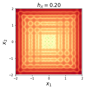
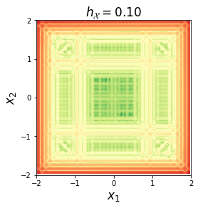
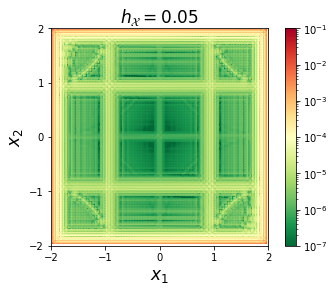
Figure 1. $L^{\infty}$-error for the approximant $\widehat{\mathcal{K}}_{A}^{\mathcal{Y}}=S_{\mathcal{X}}\mathcal{K}_{A}S_{\mathcal{Y}}$ for the Duffing oscillator at smoothness degree $k=1$, fill distances $h_{\mathcal{X}}\in\{0.2,0.1,0.05\}$ and $h_{\mathcal{Y}}=h_{\mathcal{X}}$.

Table 2. Case $\mathcal{Y}=\mathcal{X}$: Maximum errors for the predicted dynamics of the Duffing oscillator for the approximation $S_{\mathcal{X}}\mathcal{K}_{A}S_{\mathcal{X}}$ for four different fill distances and three different smoothness degrees.

$k$ / $h_{\mathcal{X}}$	0.2	0.1	0.05	0.025
1	2.05147	1.91387	1.82118	1.76882
2	2.29052	2.03404	1.84288	1.72993
3	2.52979	2.21211	1.92156	1.73675

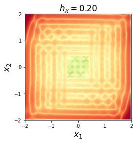
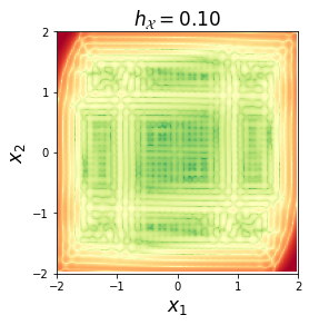
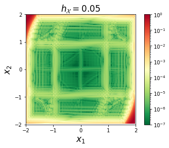
Figure 2. Case $\mathcal{Y}=\mathcal{X}$: Absolute approximation error for the approximant $S_{\mathcal{X}}\mathcal{K}_{A}S_{\mathcal{X}}$ for the Duffing oscillator at smoothness degree $k=1$, fill distances $h_{\mathcal{X}}\in\{0.2,0.1,0.05\}$ and $h_{\mathcal{Y}}=h_{\mathcal{X}}$.

6.2. Lorenz system

In a second numerical experiment, we consider the chaotic Lorenz 69 system, which is given by

$$\dot{x}_{1} =\sigma(x_{2}-x_{1}),$$

$$\dot{x}_{2} =x_{1}(\rho-x_{3})-x_{2},$$ (6.2)

$$\dot{x}_{3} =x_{1}x_{2}-\beta x_{3},$$

where $\sigma=10$, $\rho=28$, and $\beta=8/3$. Here, we let $\Omega_{X}=(-0.5,0.5)^{3}$ and fill the domain with four different meshes with mesh sizes $h_{\mathcal{X}}\in\{0.2,0.1,0.05,0.025\}$ as before, but this time in three dimensions. After simulating the flow, the domain $\Omega_{Y}$ is chosen as the smallest box including all propagated points. The validation grid is again chosen as the union of the centers of the cube cells defined by the $\mathcal{X}$-grid in order to keep the maximum distance from the interpolation points.

The results are collected in Table 3. Contrary to the previous example, where the performance of the two proposed methods was similar, we observe that in particular for large fill distances, the approximation with $S_{\mathcal{X}}\mathcal{K}_{A}$ leads to smaller errors compared to $S_{\mathcal{X}}\mathcal{K}_{A}S_{\mathcal{Y}}$.

Table 3. Maximum errors of the predicted dynamics of the Lorenz 69 model for the approximations $S_{\mathcal{X}}\mathcal{K}_{A}$ (left) and $S_{\mathcal{X}}\mathcal{K}_{A}S_{\mathcal{Y}}$ (right) for four different fill distances and three different smoothness degrees

$k$ / $h_{\mathcal{X}}$	0.2	0.1	0.05	0.025
1	0.06793	0.01497	0.00316	0.00069
2	0.07461	0.00945	0.00097	0.00009
3	0.09688	0.00821	0.00047	0.00002

$k$ / $h_{\mathcal{X}}$	0.2	0.1	0.05	0.025
1	0.22827	0.06824	0.01666	0.00073
2	0.27389	0.07084	0.01024	0.00009
3	0.28858	0.08690	0.00840	0.00002

7. Conclusions

We have shown in Proposition 5 that the kernel EDMD approximant of the Koopman operator $\mathcal{K}_{\mathcal{A}}$ – typically defined as the solution of a linear regression problem – may be equivalently expressed as a compression in native spaces by using interpolation operators. Based on this novel representation, we derived the first uniform finite-data error estimates for kEDMD. This enabled us to prove convergence in the infinite-data limit with convergence rates depending on the smoothness of the dynamics in Theorem 15. To this end, we have rigorously shown invariance of a rich class of fractional Sobolev spaces under the Koopman operator – a key property leveraged in the subsequent analysis. These are generated by Wendland kernels (compactly-supported radial basis functions of minimal degree) and are particularly attractive from a numerical perspective [30].

Appendix A Conditions on the boundary of a bounded domain

In this paper, we consider several conditions on the regularity of the boundary of a bounded domain $\Omega\subset\mathbb{R}^{d}$. Recall that a domain is a non-empty connected open set.

Definition 17.

Let $\Omega\subset\mathbb{R}^{d}$ be a bounded domain.

1. ([1, §4.9]) We say that $\Omega$ has a Lipschitz boundary if for every $x\in\partial\Omega$ there is a neighborhood $U_{x}$ of $x$ such that $U_{x}\cap\partial\Omega$ is the graph of a Lipschitz-continuous function, i.e. there exist a Lipschitz-continuous function $\varphi:\mathbb{R}^{d-1}\to\mathbb{R}$ and a rigid motion (i.e., a rotation plus a translation) $T:\mathbb{R}^{d}\to\mathbb{R}^{d}$ such that

   $$U_{x}\cap\Omega=U_{x}\cap\big{\{}T(y):y\in\mathbb{R}^{d},\,y_{d}<\varphi(y_{1},\ldots,y_{d-1})\big{\}}.$$

2. ([13]) $\Omega$ satisfies the uniform cone condition if there exists a locally finite countable open cover $\{U_{j}\}$ of the boundary of $\Omega$ and a corresponding sequence $\{C_{j}\}$ of finite cones, each congruent to some fixed finite cone $C$, such that

   1. There exists $M>0$ such that every $U_{j}$ has diameter less then $M$

   2. $\{x\in\Omega:\operatorname{dist}(x,\partial\Omega)<\delta\}\subset\bigcup_{j}U_{j}$ for some $\delta>0$

   3. $Q_{j}:=\bigcup_{x\in\Omega\cap U_{j}}(x+C_{j})\subset\Omega$ for every $j$

   4. For some finite $R$, every collection of $R+1$ of the sets $Q_{j}$ has empty intersection.

3. ([30, Definition 3.6]) $\Omega$ satisfies the interior cone condition if there are an angle $\theta\in(0,\pi/2)$ and a radius $r>0$ such that the following holds: for every $x\in\Omega$ there exists $\xi(x)\in\mathbb{R}^{d}$, $\|\xi(x)\|_{2}=1$, such that the cone

   $$C\big{(}x,\xi(x),\theta,r\big{)}:=\{x+\lambda y:y\in\mathbb{R}^{d},\,\|y\|=1,\,y^{\top}\xi(x)\geq\cos\theta,\,\lambda\in[0,r]\}$$

   is contained in $\Omega$.

In Theorem 10, the domain needs to have a Lipschitz boundary in the sense of [3, Definition 1.4.4], which, on bounded domains, is easily seen to be implied by the Lipschitz condition above. To obtain the interpolation estimates in Theorem 14, the interior cone condition is needed, which is precisely the cone condition from [1, Paragraph 4.6] and is implied by the Lipschitz boundary condition (see [1, Paragraph 4.11]).

Appendix B Bounds on the Koopman operator norm

In this section, we prove explicit bounds on the operator norms $\|\mathcal{K}_{A}\|_{H^{\sigma}(\Omega_{Y})\to H^{\sigma}(\Omega_{X})}$ for $\sigma\in\mathbb{N}$. We denote by $\mathcal{L}^{k}(\mathbb{R}^{d},\mathbb{R}^{n})$ the linear space of all $k$-multilinear mappings $\Psi:(\mathbb{R}^{d})^{k}\to\mathbb{R}^{n}$. A multilinear map $\Psi\in\mathcal{L}^{k}(\mathbb{R}^{d},\mathbb{R}^{n})$ is called symmetric if $\Psi(Pv)=\Psi(v)$ for any permutation matrix $P\in\mathbb{R}^{d\times d}$ and all $v\in(\mathbb{R}^{d})^{k}$. By $\mathcal{L}_{s}^{k}(\mathbb{R}^{d},\mathbb{R}^{n})$ we denote the set of all symmetric $k$-multilinear maps.

For the $k$-th total derivative $\mathcal{D}^{k}A$ of $A:\Omega_{X}\to\Omega_{Y}$ we have $\mathcal{D}^{k}A(x)\in\mathcal{L}^{k}_{s}(\mathbb{R}^{d},\mathbb{R}^{d})$, $x\in\Omega_{X}$, by setting

$$\mathcal{D}^{k}A(x)(e_{i_{1}},\ldots,e_{i_{k}})=\partial_{i_{1}}\cdots\partial_{i_{k}}A(x),$$

where $e_{i}$ denotes the $i$-th standard basis vector. For scalar-valued $f:\Omega_{Y}\to\mathbb{R}$ we have accordingly $f^{(k)}(y):=\mathcal{D}^{k}f(y)\in\mathcal{L}^{k}_{s}(\mathbb{R}^{d},\mathbb{R})$. For example, the second derivative of $f$ can be written as $f^{(2)}(y)(x_{1},x_{2})=x_{1}^{\top}H_{f}(y)x_{2}$, where $H_{f}(y)$ denotes the Hessian of $f$ at $y$.

For $\sigma\in\mathbb{N}$ we denote the set of all partitions $\pi$ of $\{1,\dots,\sigma\}$ by $\Pi_{\sigma}$. For a partition $\pi\in\Pi_{\sigma}$, $\left\lvert\pi\right\rvert$ denotes the number of blocks $B$ in the partition $\pi$.

For $\alpha\in\mathbb{N}_{0}^{d}$, we denote by $\mathcal{P}(\alpha)$ the set of all vectors $\beta\in[1:d]^{|\alpha|}$ in which any index $k\in[1:d]$ appears exactly $\alpha_{k}$ times. For example, for $\alpha=(2,1)$ we have $\mathcal{P}(\alpha)=\{(1,1,2),(1,2,1),(2,1,1)\}$.

Theorem 18.

Let $\sigma\in\mathbb{N}$, and assume in addition that $A\in C_{b}^{\sigma}(\Omega_{X},\mathbb{R}^{d})$. Then we have

$$\left\lVert\operatorname{\mathcal{K}_{A}}\right\rVert_{H^{\sigma}({Y})\to H^{\sigma}({X})}\leq\bigg{(}\max\bigg{\{}c_{0},\sum_{1\leq|\alpha|\leq\sigma}S_{\alpha}(A)\bigg{\}}\bigg{)}^{1/2},$$

where $c_{0}:=\sup_{x\in\Omega_{X}}|\det DA(x)|^{-1}$, and for $\alpha\in\mathbb{N}_{0}^{d}$, $|\alpha|=m$, and any $\beta\in\mathcal{P}(\alpha)$,

$$S_{\alpha}(A):=\sup_{x\in\Omega_{X}}|\det DA(x)|^{-1}\sum_{k=1}^{m}\sum_{|\alpha^{\prime}|=k}\Bigg{|}\sum_{\begin{subarray}{c}\pi\in\Pi_{m}\\ |\pi|=k\end{subarray}}\sum_{\beta^{\prime}\in\mathcal{P}(\alpha^{\prime})}\partial_{\beta,B_{1}}A_{\beta^{\prime}_{1}}(x)\cdots\partial_{\beta,B_{k}}A_{\beta^{\prime}_{k}}(x)\Bigg{|}^{2}.$$

Here, $B_{i}$ denotes the $i$-th block of the partition $\pi$, and $\partial_{\beta,B}$ stands for the operator $\partial_{\beta_{j_{1}}}\cdots\partial_{\beta_{j_{\ell}}}$, where $B=\{j_{1},\ldots,j_{\ell}\}$.

Proof.

We prove by induction over $\sigma\in\mathbb{N}$ that for $f\in H^{\sigma}(\Omega_{Y})$ we have

$$\|\mathcal{K}_{A}f\|_{H^{\sigma}(\Omega_{X})}^{2}\,\leq\,c_{0}\|f\|_{L^{2}(\Omega_{Y})}^{2}+\sum_{k=1}^{\sigma}\bigg{(}\sum_{k\leq|\alpha|\leq\sigma}S_{\alpha}(A)\bigg{)}\sum_{|\gamma|=k}\|D^{\gamma}f\|_{L^{2}(\Omega_{Y})}^{2}.$$ (B.1)

Then the statement of the theorem follows immediately. The anchor for eq. B.1 has been set in the first step of the proof of Theorem 11, where it was shown that $\|\mathcal{K}_{A}\|_{L^{2}(\Omega_{Y})\to L^{2}(\Omega_{X})}^{2}\leq c_{0}$. Next, let $\sigma\in\mathbb{N}$, $\sigma\geq 1$. For any $\alpha\in\mathbb{N}_{0}^{d}$ with $|\alpha|=\sigma$, we have $D^{\alpha}=\partial_{\beta}$ with some (any) $\beta\in\mathcal{P}(\alpha)$. Now, consider Faà di Bruno’s formula in combinatorial form (see [14, p. 219]):

$$(f\circ A)^{(\sigma)}(x)(z_{1},\ldots,z_{\sigma})=\sum_{\pi\in\Pi_{\sigma}}f^{({\left\lvert\pi\right\rvert})}(A(x))\big{(}\mathcal{D}^{\left\lvert B_{1}\right\rvert}A(x)(z_{B_{1}}),\dots,\mathcal{D}^{\left\lvert B_{|\pi|}\right\rvert}A(x)(z_{B_{|\pi|}})\big{)},$$

where $z_{B_{j}}\in(\mathbb{R}^{d})^{|B_{j}|}$ are the components of $(z_{1},\ldots,z_{\sigma})$ with indices in the block $B_{j}$. If we denote $e^{\beta}=(e_{\beta_{1}},\ldots,e_{\beta_{\sigma}})$, then

$$D^{\alpha}(f\circ A)(x) =\partial_{\beta}(f\circ A)(x)=(f\circ A)^{(\sigma)}(x)(e^{\beta})$$

$$=\sum_{k=1}^{\sigma}\sum_{\begin{subarray}{c}\pi\in\Pi_{\sigma}\\ |\pi|=k\end{subarray}}f^{(k)}(A(x))\big{(}\mathcal{D}^{\left\lvert B_{1}\right\rvert}A(x)(e^{\beta}_{B_{1}}),\dots,\mathcal{D}^{\left\lvert B_{k}\right\rvert}A(x)(e^{\beta}_{B_{k}})\big{)}$$

$$=\sum_{k=1}^{\sigma}\sum_{\begin{subarray}{c}\pi\in\Pi_{\sigma}\\ |\pi|=k\end{subarray}}f^{(k)}(A(x))\big{(}\partial_{\beta,B_{1}}A(x),\dots,\partial_{\beta,B_{k}}A(x)\big{)}$$

$$=\sum_{k=1}^{\sigma}\sum_{\begin{subarray}{c}\pi\in\Pi_{\sigma}\\ |\pi|=k\end{subarray}}\sum_{\beta^{\prime}\in[1:d]^{k}}\partial_{\beta,B_{1}}A_{\beta^{\prime}_{1}}(x)\cdots\partial_{\beta,B_{k}}A_{\beta^{\prime}_{k}}(x)\cdot f^{(k)}(A(x))(e^{\beta^{\prime}})$$

$$=\sum_{k=1}^{\sigma}\sum_{\begin{subarray}{c}\pi\in\Pi_{\sigma}\\ |\pi|=k\end{subarray}}\sum_{\beta^{\prime}\in[1:d]^{k}}\partial_{\beta,B_{1}}A_{\beta^{\prime}_{1}}(x)\cdots\partial_{\beta,B_{k}}A_{\beta^{\prime}_{k}}(x)\cdot\partial_{\beta^{\prime}}f(A(x))$$

$$=\sum_{k=1}^{\sigma}\sum_{|\alpha^{\prime}|=k}D^{\alpha^{\prime}}f(A(x))\underbrace{\sum_{\begin{subarray}{c}\pi\in\Pi_{\sigma}\\ |\pi|=k\end{subarray}}\sum_{\beta^{\prime}\in\mathcal{P}(\alpha^{\prime})}\partial_{\beta,B_{1}}A_{\beta^{\prime}_{1}}(x)\cdots\partial_{\beta,B_{k}}A_{\beta^{\prime}_{k}}(x)}_{=:A_{\alpha,k,\alpha^{\prime}}(x)}.$$

Thus, we have $D^{\alpha}(f\circ A)=\sum_{k=1}^{\sigma}\sum_{|\alpha^{\prime}|=k}[(D^{\alpha^{\prime}}f)\circ A]\cdot A_{\alpha,k,\alpha^{\prime}}$, and we estimate

$$\|D^{\alpha}(f\circ A)\|_{L^{2}(\Omega_{X})}^{2} =\int_{\Omega_{X}}\bigg{(}\sum_{k,\alpha^{\prime}}[(D^{\alpha^{\prime}}f)\circ A]\cdot A_{\alpha,k,\alpha^{\prime}}\bigg{)}^{2}\,dx$$

$$=\int_{\Omega_{Y}}\bigg{(}\sum_{k,\alpha^{\prime}}(D^{\alpha^{\prime}}f)\cdot[A_{\alpha,k,\alpha^{\prime}}\circ A^{-1}]\bigg{)}^{2}|\det DA^{-1}|\,dy$$

$$=\int_{\Omega_{Y}}\bigg{(}\sum_{k,\alpha^{\prime}}(D^{\alpha^{\prime}}f)\cdot\underbrace{[A_{\alpha,k,\alpha^{\prime}}\circ A^{-1}]|\det DA^{-1}|^{1/2}}_{=:\widetilde{A}_{\alpha,k,\alpha^{\prime}}}\bigg{)}^{2}\,dy$$

$$\leq\int_{\Omega_{Y}}\bigg{(}\sum_{k,\alpha^{\prime}}|D^{\alpha^{\prime}}f|^{2}\bigg{)}\bigg{(}\sum_{k,\alpha^{\prime}}|\widetilde{A}_{\alpha},{k,\alpha^{\prime}}|^{2}\bigg{)}\,dy$$

$$\leq\bigg{(}\sup_{y\in\Omega_{Y}}\sum_{k,\alpha^{\prime}}|\widetilde{A}_{\alpha,k,\alpha^{\prime}}(y)|^{2}\bigg{)}\bigg{(}\sum_{k,\alpha^{\prime}}\int_{\Omega_{Y}}|D^{\alpha^{\prime}}f|^{2}\,dy\bigg{)}$$

$$\leq\bigg{(}\sup_{x\in\Omega_{X}}\sum_{k,\alpha^{\prime}}\frac{|A_{\alpha,k,\alpha^{\prime}}(x)|^{2}}{|\det DA(x)|}\bigg{)}\sum_{1\leq|\gamma|\leq\sigma}\|D^{\gamma}f\|_{L^{2}(\Omega_{Y})}^{2}$$

$$=S_{\alpha}(A)\sum_{1\leq|\gamma|\leq\sigma}\|D^{\gamma}f\|_{L^{2}(\Omega_{Y})}^{2}.$$

Therefore, we obtain by assumption that

$$\|\mathcal{K}_{A}f\|_{H^{\sigma}(\Omega_{X})}^{2} =\|\mathcal{K}_{A}f\|_{H^{\sigma-1}(\Omega_{X})}^{2}+\sum_{|\alpha|=\sigma}\|D^{\alpha}(f\circ A)\|_{L^{2}(\Omega_{X})}^{2}$$

$$\leq c_{0}\|f\|_{L^{2}(\Omega_{Y})}^{2}+\sum_{k=1}^{\sigma-1}\bigg{(}\sum_{k\leq|\alpha|\leq\sigma-1}S_{\alpha}(A)\bigg{)}\sum_{|\gamma|=k}\|D^{\gamma}f\|_{L^{2}(\Omega_{Y})}^{2}$$

$$\hskip 70.27834pt+\sum_{|\alpha|=\sigma}S_{\alpha}(A)\sum_{1\leq|\gamma|\leq\sigma}\|D^{\gamma}f\|_{L^{2}(\Omega_{Y})}^{2}$$

$$=c_{0}\|f\|_{L^{2}(\Omega_{Y})}^{2}+\sum_{k=1}^{\sigma}\bigg{(}\sum_{k\leq|\alpha|\leq\sigma}S_{\alpha}(A)\bigg{)}\sum_{|\gamma|=k}\|D^{\gamma}f\|_{L^{2}(\Omega_{Y})}^{2},$$

as we wished to prove. ∎

In the particular case $\sigma=1$, Theorem 18 yields the following corollary.

Corollary 19.

We have

$$\left\lVert\operatorname{\mathcal{K}_{A}}\right\rVert_{H^{1}(\Omega_{Y})\to H^{1}(\Omega_{X})}\leq\max\bigg{\{}c_{0},\sup_{x\in\Omega_{X}}\frac{\|DA(x)\|_{F}^{2}}{|\det DA(x)|}\bigg{\}}^{1/2}.$$

Remark 20.

In fact, it is not hard to see that the Frobenius norm $\|DA(x)\|_{F}$ above can be replaced by the spectral norm $\|DA(x)\|_{2\to 2}$ (cf. [11]).

References

• [1] RobertΒ A Adams and John JΒ F Fournier. Sobolev spaces, volume 140. Elsevier/Academic Press, Amsterdam, second edition, 2003.
• [2] Omri Azencot, NΒ Benjamin Erichson, Vanessa Lin, and Michael Mahoney. Forecasting sequential data using consistent Koopman autoencoders. In International Conference on Machine Learning, pages 475–485. PMLR, 2020.
• [3] SusanneΒ C Brenner and LΒ R Scott. The Mathematical Theory of Finite Element Methods. Springer New York, 2008.
• [4] BingniΒ W Brunton, LiseΒ A Johnson, JeffreyΒ G Ojemann, and JΒ Nathan Kutz. Extracting spatial–temporal coherent patterns in large-scale neural recordings using dynamic mode decomposition. Journal of Neuroscience Methods, 258:1–15, 2016.
• [5] StevenΒ L. Brunton, Marko BudiΕ‘iΔ‡, Eurika Kaiser, and J.Β Nathan Kutz. Modern Koopman Theory for Dynamical Systems. SIAM Review, 64(2):229–340, 2022.
• [6] SΒ N Chandler-Wilde, DΒ P Hewett, and AΒ Moiola. Interpolation of Hilbert and Sobolev spaces: quantitative estimates and counterexamples. Mathematika, 61:414–443, 2015.
• [7] MΒ J Colbrook, QΒ Li, RΒ V Raut, and AΒ Townsend. Beyond expectations: residual dynamic mode decomposition and variance for stochastic dynamical systems. Nonlinear Dynamics, 112:2037–2061, 2024.
• [8] AkshunnaΒ S Dogra and William Redman. Optimizing neural networks via Koopman operator theory. Advances in Neural Information Processing Systems, 33:2087–2097, 2020.
• [9] GEΒ Fasshauer. Meshfree methods. Handbook of Theoretical and Computational Nanotechnology, 27:33–97, 2005.
• [10] Dimitrios Giannakis, Anastasiya Kolchinskaya, Dmitry Krasnov, and JΓΆrg Schumacher. Koopman analysis of the long-term evolution in a turbulent convection cell. Journal of Fluid Mechanics, 847:735–767, 2018.
• [11] VΒ Gol’dshtein, LΒ Gurov, and AΒ Romanov. Homeomorphisms that induce monomorphisms of Sobolev spaces. Israel Journal of Mathematics, 91:31–60, 1995.
• [12] Efrain Gonzalez, Moad Abudia, Michael Jury, Rushikesh Kamalapurkar, and JoelΒ A. Rosenfeld. The kernel perspective on dynamic mode decomposition. Preprint, arxiv:2106.00106, 2023.
• [13] MΒ Hegland and JΒ T Marti. Numerical computation of least constants for the Sobolev inequality. Numerische Mathematik, 48(6):607–616, November 1986.
• [14] Warren Johnson. The curious history of Faa di Bruno’s formula. American Mathematical Monthly, 109:217–234, 03 2002.
• [15] Stefan Klus, Feliks NΓΌske, and Boumediene Hamzi. Kernel-based approximation of the Koopman generator and SchrΓΆdinger operator. Entropy, 22(7):722, 2020.
• [16] BΒ O Koopman. Hamiltonian systems and transformation in Hilbert space. Proceedings of the National Academy of Sciences of the United States of America, 17:315, 1931.
• [17] Milan Korda and Igor MeziΔ‡. On convergence of extended dynamic mode decomposition to the Koopman operator. J. Nonlinear Science, 28(2):687–710, 2018.
• [18] WΒ McLean. Strongly Elliptic Systems and Boundary Integral Equations. Cambridge University Press, 2000.
• [19] I.Β MeziΔ‡. On numerical approximations of the Koopman operator. Mathematics, 10:1180, 2022.
• [20] Igor MeziΔ‡. Spectral properties of dynamical systems, model reduction and decompositions. Nonlinear Dynamics, 41(1-3):309–325, 2005.
• [21] Igor MeziΔ‡. Analysis of fluid flows via spectral properties of the Koopman operator. Annual Review of Fluid Mechanics, 45:357–378, 2013.
• [22] F.Β NΓΌske, S.Β Peitz, F.Β Philipp, M.Β Schaller, and KΒ Worthmann. Finite-data error bounds for Koopman-based prediction and control. Journal of Nonlinear Science, 33:14, 2023.
• [23] VΒ I Paulsen and MΒ Raghupathi. An Introduction to the Theory of Reproducing Kernel Hilbert Spaces. Cambridge University Press, 2016.
• [24] FΒ M Philipp, Manuel Schaller, SΒ Boshoff, Sebastian Peitz, Feliks NΓΌske, and Karl Worthmann. Extended dynamic mode decomposition: Sharp bounds on the sample efficiency. Preprint, arXiv:2402.02494, 2024.
• [25] Friedrich Philipp, Manuel Schaller, Karl Worthmann, Sebastian Peitz, and Feliks NΓΌske. Error analysis of kernel EDMD for prediction and control in the Koopman framework. Preprint, arxiv:2312.10460, 2023.
• [26] Friedrich Philipp, Manuel Schaller, Karl Worthmann, Sebastian Peitz, and Feliks NΓΌske. Error bounds for kernel-based approximations of the Koopman operator. Preprint, arxiv:2301.08637, 2023.
• [27] Manuel Schaller, Karl Worthmann, Friedrich Philipp, Sebastian Peitz, and Feliks NΓΌske. Towards reliable data-based optimal and predictive control using extended DMD. IFAC-PapersOnLine, 56(1):169–174, 2023.
• [28] IΒ Steinwart and AΒ Christmann. Support Vector Machines. Springer Science+Business Media, LLC, 2008.
• [29] Luc Tartar. An Introduction to Sobolev Spaces and Interpolation Spaces (Lecture Notes of the Unione Matematica Italiana). Springer, 2007.
• [30] Holger Wendland. Scattered data approximation, volumeΒ 17. Cambridge university press, 2004.
• [31] MΒ O Williams, CΒ W Rowley, and IΒ Kevrekidis. A kernel-based method for data-driven Koopman spectral analysis. Journal of Computational Dynamics, 2:247–265, 2015.
• [32] Hao Wu, Feliks NΓΌske, Fabian Paul, Stefan Klus, PΓ©ter Koltai, and Frank NoΓ©. Variational Koopman models: Slow collective variables and molecular kinetics from short off-equilibrium simulations. The Journal of Chemical Physics, 146(15), 2017.
• [33] Rishikesh Yadav and Alexandre Mauroy. Approximation of the Koopman operator via bernstein polynomials. arXiv preprint arXiv:2403.02438, 2024.
• [34] C.Β Zhang and E.Β Zuazua. A quantitative analysis of Koopman operator methods for system identification and predictions. Comptes Rendus MΓ©canique, 351:1–31, 2023.