Evaluation of transition rates from nonequilibrium instantons

Abstract

Equilibrium rate theories play a crucial role in understanding rare, reactive events. However, they are inapplicable to a range of irreversible processes in systems driven far from thermodynamic equilibrium like active and biological matter. Here, we develop a general, computationally efficient nonequilibrium rate theory in the weak-noise limit based on an instanton approximation to the stochastic path integral and illustrate its wide range of application in the study of rare nonequilibrium events. We demonstrate excellent agreement of the instanton rates with numerically exact results for a particle under a non-conservative force. We also study phase transitions in an active field theory. We elucidate how activity alters the stability of the two phases and their rates of interconversion in a manner that can be well-described by modifying classical nucleation theory.

Unlike their equilibrium counterparts, rare nonequilibrium transitions are not governed by the energetics of static transition states. This renders efficient equilibrium techniques for computing rates and elucidating mechanisms largely invalid. Instead, reaction rates in systems driven far from thermodynamic equilibrium are dependent on the details of their trajectories. This is formalized by Freidlin–Wentzell theory in the weak-noise limit with the optimal transition path or instanton [1, 2, 3]. Instantons have recently emerged as a powerful computational tool, offering insights into a wide variety of nonequilibrium phenomena across diverse disciplines like fluid dynamics, soft active matter, biology, and chemistry [4, 5, 6, 7, 8, 9, 10, 11, 12, 13, 14, 15]. In this work, we develop a rigorous, numerically efficient nonequilibrium instanton rate theory (NEQI) that provides a quantitative understanding of transitions in complex driven systems. We show the instanton rates computed with our method are in excellent agreement with numerically exact results at weak noise for a particle under a non-gradient force and illustrate dramatic changes of transition rates and mechanisms due to nonequilibrium driving. Further, we apply our method to an active field theory relevant to the study of how phase transforms are altered in the presence of active forces, revealing how insights from classical nucleation theory can be recovered even in nonequilibrium phase transitions [16, 17, 18].

We consider a system with position vector $\mathsf{x}=\{x_{1},...,x_{f}\}$ described by overdamped Brownian motion

$$\dot{\mathsf{x}}(t)=\mathbf{\mu}\mathsf{F}[\mathsf{x}(t)]+\sqrt{2\epsilon}\,\mathbf{\Lambda}\,\eta(t),$$ (1)

where $\dot{\mathsf{x}}(t)=\mathrm{d}\mathsf{x}/\mathrm{d}t$, $\mathsf{F}[\mathsf{x}(t)]$ is the sum of conservative and non-conservative forces exerted on the system, $\mathbf{D}=\mathbf{\Lambda}\mathbf{\Lambda}^{\!\text{T}}$ is a non-singular diffusion matrix, and $\mathbf{\mu}=\beta\epsilon\mathbf{D}$ is the mobility matrix at inverse temperature $\beta=1/k_{\text{B}}T$. The stochastic white noise, $\eta(t)$, defined via $\braket{\eta_{i}(t)}=0$ and $\braket{\eta_{i}(t)\eta_{j}(t^{\prime})}=\delta_{ij}\delta(t-t^{\prime})$, where $i,j\in[1,f]$, has a scale denoted by $\epsilon$. We examine rate problems, where, in the absence of the nonequilibrium driving, an unstable transition state (TS) at $\mathsf{x}^{\ddagger}$ lies in between the metastable reactant and product configurations at $\mathsf{x}_{\text{R}}$ and $\mathsf{x}_{\text{P}}$. All three configurations are fixed points of the force, but whereas the derivative matrix $\nabla F$ is negative definite at the reactant and product configurations, it exhibits one positive eigenvalue at the TS. This corresponds to the typical crossing of a potential-energy barrier, where an approximation to the rate is given by Kramers–Langer theory (KLT) [19, 20, 21, 22, 23, 24].

For systems driven far out of equilibrium by a non-conservative force, the steady-state probability distribution is generally not known, and KLT does not apply. Nevertheless, the exact rate constant for a transition from reactant to product can be defined via [25]

$$k =\frac{\braket{h_{\text{R}}(0)\dot{h}_{\text{P}}(t_{\text{f}})}}{\braket{h_{\text{R}}}},$$ (2)

where the brackets indicate an average over trajectories of duration $t_{\text{rel}}\ll t_{\text{f}}\ll 1/k$, and we assume the typical separation between the timescale of the system’s relaxation dynamics $t_{\text{rel}}$ and the timescale of the rare event $1/k$. The indicator functions $h_{\text{R}}=\Theta[\sigma^{\ddagger}-\sigma(\mathsf{x})]$ and $h_{\text{P}}=1-h_{\text{R}}$ define the reactant and product regions, which are separated by a dividing surface $\sigma^{\ddagger}$ along an order parameter $\sigma(\mathsf{x})$. The flux–side correlation function can be written as an integral over the dividing surface parameterized by the $(f-1)$-dimensional vector $\mathsf{s}$

$$\braket{h_{\text{R}}(0)\dot{h}_{\text{P}}(t_{\text{f}})} =\int\rho(\mathsf{x}_{\sigma},t_{\text{f}};\mathsf{x}_{\text{R}},0)\,\dot{{x}}_{\sigma}(t_{\text{f}})\,\mathrm{d}\mathsf{s},$$ (3)

where $\rho(\mathsf{x}_{\sigma},t_{\text{f}};\mathsf{x}_{\text{R}},0)$ is the joint probability density of starting at position $\mathsf{x}_{\text{R}}$ at $t=0$ and reaching the point $\mathsf{x}_{\sigma}$ on the dividing surface at time $t_{\text{f}}$, and $\dot{x}_{\sigma}=\nabla\sigma(\mathsf{x})\cdot\dot{\mathsf{x}}$ is the velocity normal to $\sigma(\mathsf{x})$. Because of the separation of timescales, the rate does not depend on the precise initial conditions as long as the probability density is concentrated within the reactant basin, which allowed the convenient choice $\rho(t=0)=\delta[\mathsf{x}(0)-\mathsf{x}_{\text{R}}]$ [26, 27, 28, 29].

The probability density in Eq. (3) can be expressed as an integral over all paths connecting $\mathsf{x}_{\text{i}}$ and $\mathsf{x}_{\text{f}}$ in time $t_{\text{f}}$,

$$\rho(\mathsf{x}_{\text{f}},t_{\text{f}};\mathsf{x}_{\text{i}},0) =\int_{\mathsf{x}(0)=\mathsf{x}_{\text{i}}}^{\mathsf{x}(t_{\text{f}})=\mathsf{x}_{\text{f}}}\mathrm{e}^{-S[\mathsf{x}(t)]/\epsilon}\,\mathcal{D}[\mathsf{x}(t)],$$ (4)

each of which is exponentially weighted by its Onsager–Machlup action $S[\mathsf{x}]=\int_{0}^{t_{\text{f}}}\mathcal{L}(\mathsf{x},\dot{\mathsf{x}})\,\mathrm{d}t$ [2, 3, 1], where the time-dependence of positions and velocities is implied, and the Lagrangian is given by

$$\mathcal{L}(\mathsf{x},\dot{\mathsf{x}}) =\frac{1}{4}[\dot{\mathsf{x}}-\mathbf{\mu}\mathsf{F}(\mathsf{x})]^{\text{T}}\mathbf{D}^{-1}\,[\dot{\mathsf{x}}-\mathbf{\mu}\mathsf{F}(\mathsf{x})].$$ (5)

The exact evaluation of Eq. (4) is unfeasible for complex systems because it involves a sum over infinitely many paths. Some importance sampling methods exist to estimate it for systems away from equilibrium [30, 31]. In the weak-noise limit, however, we can use Laplace’s method to devise an efficient approximation about the minimum-action path or instanton, $\bar{\mathsf{x}}(t)$.

The instanton, which can be interpreted as the optimal transition path, constitutes the centerpiece of our rate theory. The action of the instanton is determined by its endpoints and the propagation time so that it can be written as $S\equiv S(\mathsf{x}_{\text{i}},\mathsf{x}_{\text{f}};t_{\text{f}})=\int_{0}^{t_{\text{f}}}\bar{\mathsf{p}}^{\text{T}}\!\mathbf{D}\bar{\mathsf{p}}\,\mathrm{d}t$, where $\bar{\mathsf{p}}=\mathbf{D}^{-1}[\dot{\bar{\mathsf{x}}}-\mathbf{\mu}\mathsf{F}(\bar{\mathsf{x}})]/2$ is the canonical momentum along the instanton. The Lagrangian in Eq. (5) can be Legendre transformed to obtain the corresponding Hamiltonian, whose value $E=\bar{\mathsf{p}}^{\text{T}}\mathbf{D}\bar{\mathsf{p}}+\bar{\mathsf{p}}^{\text{T}}\mathbf{\mu}\mathsf{F}(\bar{\mathsf{x}})$ is conserved along the instanton because we consider forces without explicit time dependence. The Hamilton–Jacobi formalism naturally yields the well-known relations for the instanton energy and the momentum at the endpoint [32, 33]

$$\bar{\mathsf{p}}_{\text{f}} \equiv\bar{\mathsf{p}}(t_{\text{f}})=\frac{\partial S}{\partial\mathsf{x}_{\text{f}}},\qquad\frac{\partial S}{\partial t_{\text{f}}}=-E.$$ (6)

For the Laplace approximation of the rate, we require an instanton from reactant to product that minimizes the action not only in coordinate space but also in time $t_{\text{f}}$, which is achieved when $E=0$ or equivalently $t_{\text{f}}\rightarrow\infty$. Consequently, the instanton takes the form of a “double kink” illustrated in the SI, connecting between the three fixed points of the force, even in the presence of a non-gradient force. In spite of the infinite propagation time, the action remains finite because the dwell phases do not contribute.

From the stationarity conditions $\delta S=0$ and $E=0$ follows $\dot{\bar{\mathsf{x}}}^{2}=[\mathbf{\mu}\mathsf{F}(\bar{\mathsf{x}})]^{2}$. At equilibrium, the action is directly related to the height of the potential-energy barrier because the instanton minimizes the potential along its path, thus aligning with the mobility-scaled conservative force $\mathbf{\mu}\mathsf{F}_{\text{c}}=-\mathbf{\mu}\nabla V$. Consequently, $\dot{\bar{\mathsf{x}}}=\pm\mathbf{\mu}\mathsf{F}_{\text{c}}$, where the minus sign corresponds to the activation path from reactant to TS, and the plus sign corresponds to the relaxation path, which follows the force into the product configuration. Notably, only the activation path contributes to the action. Unlike the relaxation path, which remains aligned with the force also under nonequilibrium conditions, the activation path generally deviates, leading to changes in transition rate and mechanism.

Since the relaxation path does not contribute to the rate [34], the natural choice for the location of the dividing surface is the unstable fixed point of the total force, to which we will refer as a TS. Therefore, we can focus solely on the activation path, which we henceforth call the instanton. Combining Eqs. (2), (3) and (4) leads to the path-integral representation of the rate constant

$$k\,Z_{\text{R}}=\lim_{N\rightarrow\infty}\int\frac{\dot{x}_{\sigma}(t_{\text{f}})\,\mathrm{e}^{-S_{N}/\epsilon}\,\mathrm{d}\mathsf{x}_{1}...\mathrm{d}\mathsf{x}_{N-1}\mathrm{d}\mathsf{s}}{(\text{det}[4\pi\epsilon\tau\mathbf{D}])^{N/2}},$$ (7)

where, in order to evaluate the action numerically, we discretized the paths into $N$ equal-time segments of length $\tau=t_{\text{f}}/N$. In the instanton limit, the reactant path partition function $Z_{\text{R}}$=1. The discretized action $S_{N}\equiv S_{N}(\mathsf{x}_{0},...,\mathsf{x}_{N};t_{\text{f}})$ is a function of the “beads” $\mathsf{x}_{n}$, which constitute copies of the system along the path

$$S_{N}=\frac{\tau}{4}\sum_{n=0}^{N-1}\left[\frac{\mathsf{x}_{n+1}-\mathsf{x}_{n}}{\tau}-\mathbf{\mu}F(\mathsf{x}_{n})\right]^{\text{T}}\\ \times\mathbf{D}^{-1}\left[\frac{\mathsf{x}_{n+1}-\mathsf{x}_{n}}{\tau}-\mathbf{\mu}F(\mathsf{x}_{n})\right].$$ (8)

We aim to evaluate the integrals over the beads and the dividing surface with Laplace’s method. Hence, the instanton with endpoints $\mathsf{x}_{0}=\mathsf{x}_{\text{R}}$ and $\mathsf{x}_{N}=\mathsf{x}^{\ddagger}$ must satisfy $\nabla_{\text{s}}S_{N}=0$, where $\nabla_{\text{s}}=(\partial/\partial\mathsf{x}_{1},...,\partial/\partial\mathsf{x}_{N-1},\partial/\partial\mathsf{s})$ is the gradient with respect to the positions of all intermediate beads and the parameters of the dividing surface. The optimal path can therefore be located with standard optimization algorithms [35] (see SI). From the stationarity condition $\partial S_{N}/\partial s_{i}=\bar{\mathsf{p}}_{\text{f}}\cdot\partial\mathsf{x}_{N}/\partial s_{i}=0$, we find that the momentum at the endpoint is orthogonal to the dividing surface [28]. Given that the mobility-scaled force and the instanton velocity are parallel at the TS, it follows that $\dot{\bar{x}}_{\sigma}(t_{\text{f}})=\bar{\mathsf{p}}_{\text{f}}^{\text{T}}\mathbf{D}\bar{\mathsf{p}}_{\text{f}}/\bar{p}_{\text{f}}$, where $\bar{p}_{\text{f}}=\lVert\bar{\mathsf{p}}_{\text{f}}\rVert$.

Approximating Eq. (7) by Laplace’s method now appears straightforward. However, the instanton, as an infinite-time trajectory, can dwell at the reactant or the TS for an arbitrary time without changing its action (see SI). Hence, there is an infinite number of instantons that are related by continuous time translation. This leads to the emergence of a Goldstone mode, which manifests itself as a zero eigenvalue in the second-derivative matrix of the action, $\nabla_{\text{s}}^{2}S_{N}$, and thus cannot be integrated over by Laplace’s method. Previous work avoided this difficulty by considering explicitly time-dependent forces that break time-translation symmetry [26, 27, 28].

However, progress can be made by noting that a small translation along the zero mode can be related to a time translation of the instanton, $\mathrm{d}\zeta_{0}=\sqrt{B_{t}/\tau}\,\mathrm{d}t^{\prime}$ [36, 34], where $B_{t}=\int\dot{\bar{\mathsf{x}}}^{2}\,\mathrm{d}t$ is a normalization constant . This allows us to transform the integral over the Goldstone mode to an integral over a collective time, e.g., the time to reach the TS. By noting that the prefactor $\bar{\mathsf{p}}_{\text{f}}^{\text{T}}\mathbf{D}\bar{\mathsf{p}}_{\text{f}}$ is identical to the instanton energy [Eq. (6)], this time integral is readily solved by substitution, leading to the nonequilibrium instanton formula for the rate constant

$$k \sim\frac{1}{4\pi\,\tau}\sqrt{\frac{B_{t}}{\tau\bar{p}_{\text{f}}^{2}\Sigma}}\,\mathrm{e}^{-S_{N}/\epsilon},$$ (9)

where $\Sigma=\det^{\prime}[2\tau\nabla^{2}_{\text{s}}S_{N}](\text{det}[\mathbf{D}])^{N}$ encodes fluctuations around the optimal path and the prime indicates omission of the zero eigenvalue. In contrast to the numerical derivatives in path space implied by the rate equation in Ref. 38, all quantities in Eq. (9) are efficiently evaluated from a single path, the instanton. By construction, Eq. (9) becomes exact in the limit $\epsilon\rightarrow 0$ and reduces to KLT at equilibrium .

The instanton rate is defined in the infinite-time limit. In practice, the propagation time is extended until convergence is reached, while ensuring convergence also with respect to the number of beads (see SI for details). Note that because $\Sigma\propto\bar{p}_{\text{f}}^{\,-2}$ [26, 28], the term $\bar{p}_{\text{f}}^{2}\Sigma$ can be treated as a slowly varying prefactor despite $\bar{p}_{\text{f}}$ going to zero in the infinite-time limit [40, 41]. We can leverage the banded structure of $\nabla^{2}_{\text{s}}S$ to reduce memory requirements and the scaling of the diagonalization to $\mathcal{O}(N^{2})$. In the SI, we derive an equivalent instanton rate formula in the “trajectory formalism” [42], which further reduces this scaling to $\mathcal{O}(N)$ [43, 44, 45, 36, 46, 33] and lends itself to solutions with matrix Riccati type equations [47, 48, 49, 50, 28].

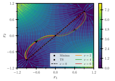
Figure 1: Instantons at different values of $\nu$ on a color map of the potential defined in the text and a stream plot depicting the conservative force field. The forward (solid) and backward (transparent) instantons, whose direction is indicated by the black arrows, do not coincide out of equilibrium ($\nu\neq 0$).

We apply our new method to a model system in two dimensions with total force

$$\mathsf{F}(\mathsf{x}) =-\frac{\partial V(\mathsf{x})}{\partial\mathsf{x}}+\nu\begin{pmatrix}x_{-}^{3}-x_{-}\\ x_{-}^{3}-x_{-}\end{pmatrix},$$ (10)

where $x_{\pm}=x_{1}\pm x_{2}$, and the non-conservative force is scaled by the driving strength $\nu$. We consider the potential $V(\mathsf{x})=A(x_{+}^{2}-B^{2})^{2}/B^{4}+x_{-}^{2}$ with $A=2$ and $B=1.8$, and set $\mathbf{\mu}=\mathbf{D}=\mathbb{I}$ for simplicity, where $\mathbb{I}$ is the identity matrix. In Fig. 1, we illustrate how nonequilibrium driving alters the transition mechanism. At equilibrium, the instanton follows the minimum-potential pathway along $x_{+}$, whereas the activation paths in the driven systems are curved, thus achieving a lower action. It can be seen that the forward and backward instantons lie on top of one another at equilibrium, in agreement with semiclassical instanton theories based on linear response [36, 51, 52]. Conversely, the forward and backward transition mechanisms generally differ for driven processes ($\nu>0$) because they break detailed balance.

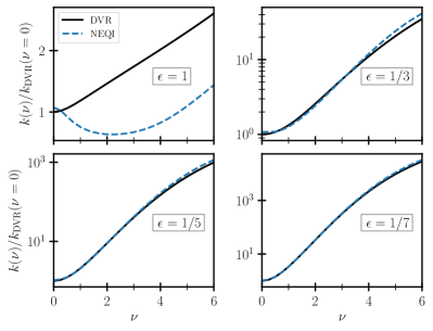
Figure 2: Rate constants for the model defined in Eq. (10) over a range of noise strengths $\epsilon$ and driving strengths $\nu$ computed from nonequilibrium instanton theory (NEQI) and a numerically exact discrete variable representation (DVR) of the Fokker–Planck operator. For each $\epsilon$, the results are given relative to the DVR equilibrium rate ($\nu=0$).

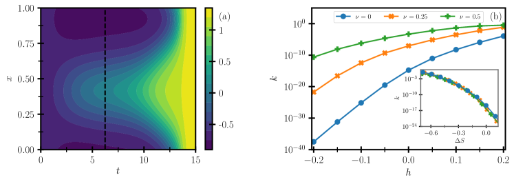
Figure 3: Instanton results for the active field theory defined in the text with parameters $\kappa=0.01$, $u=1/4$, $a=-1/2$, $\mu=1$. (a) Instanton at $h=0.1$ and $\nu=0.5$, where the color map shows the configuration of the field $\phi$ as a function of space and time along the path. The phase transition proceeds from the uniform reactant state ($\phi\approx-0.71$) to the uniform product state ($\phi\approx 1.32$) via a non-uniform TS, whose location is indicated by the dashed line. At the TS, part of the field extends towards the product, forming a critical nucleus. (b) Instanton rate constants over a range of applied fields $h$ and driving strengths $\nu$ with $\epsilon=5\cdot 10^{-3}$. The inset shows the same rate constants as a function of the difference between the instanton actions of the forward and the backward processes, $\Delta S$.

We present the rate constants computed from these instantons for various values of the noise strength in Fig. 2 alongside numerically exact results from a discrete variable representation of the Fokker–Planck operator [53, 54, 55]. Generically, the transition rate increases with the addition of the nonequilibrium driving, consistent with expectations from thermodynamic speed limits [56]. Our NEQI method captures the dramatic speed ups of the rate due to nonequilibrium driving and converges to the exact result at weak noise as expected.

To illustrate the generality of our approach, we next consider the phase transformation of a collection of active particles. Rather than consider an explicit-particle model, we employ a coarse-grained representation or active field theory known as Active model A dynamics [57, 58], which has proven fruitful in understanding the emergent phenomena of these systems on large length scales. The Langevin equation for a non-conserved scalar field $\phi$ in $f$ dimensions is

$$\dot{\phi}(\mathsf{x},t) =\mu F[\phi(\mathsf{x},t)]+\sqrt{2\epsilon}\,\eta(\mathsf{x},t),$$ (11)

where the mobility $\mu$ is constant, the white noise is defined via $\braket{\eta(\mathsf{x},t)\eta(\mathsf{x}^{\prime},t^{\prime})}=\delta(\mathsf{x}-\mathsf{x}^{\prime})\delta(t-t^{\prime})$, and $F(\phi)=-\delta V/\delta\phi+F_{\text{nc}}(\phi)$ is the drift that again contains gradient and non-gradient terms. Our nonequilibrium instanton theory directly extends to such field-theoretical descriptions, where the action,

$$S[\phi(\mathsf{x},t)] =\frac{1}{4}\int_{0}^{t_{\text{f}}}\int\left(\dot{\phi}(\mathsf{x},t)-\mu F[\phi(\mathsf{x},t)]\right)^{2}\mathrm{d}\mathsf{x}\,\mathrm{d}t,$$ (12)

must be discretized not only in time but also in space. We take the potential to be $V[\phi]=\int[\kappa\,|\nabla\phi|^{2}/2+a\phi^{2}+u\phi^{4}-h\phi]\mathrm{d}\mathsf{x}$, a sum of a square-gradient term with stiffness $\kappa$ and a free-energy density parameterized by $a<0$, $u>0$ and field $h$. The time-reversal symmetry of the system is broken by adding the strongly non-local, non-conservative force $F_{\text{nc}}[\phi(\mathsf{x})]=\nu\int\phi^{2}(\mathsf{x}^{\prime})\,\mathrm{d}\mathsf{x}^{\prime}$ [13].

An additional complication arises because transitions of fields typically involve the formation of an interface. A system with periodic boundary conditions is invariant under translation of the interface, leading to up to $f$ zero modes at the TS. However, similar to the time-translation mode, the integral over these zero modes can be transformed to an integral over space [59], where $B_{x}=\int\kappa|\nabla\phi^{\ddagger}|^{2}\,\mathrm{d}\mathsf{x}$ is the Jacobian of the transformation, and $\phi^{\ddagger}(\mathsf{x})$ is the TS configuration of the field. Along with the volume factor $\mathcal{V}$ from the integral over space, this leads to the instanton expression for the nonequilibrium rate constant in field space

$$\frac{k}{\mathcal{V}} \sim\frac{1}{4\pi\tau}\sqrt{\frac{B_{t}}{\tau\xi^{f}\bar{p}_{\text{f}}^{2}\Sigma}}\,\left(\frac{B_{x}}{4\pi\epsilon\tau\kappa}\right)^{\!f/2}\mathrm{e}^{-S_{N}/\epsilon},$$ (13)

which reduces to the field-space generalization of KLT at equilibrium [60, 59, 61]. Here, $\xi$ is the spatial resolution of the grid , and $B_{t}=\int\dot{\bar{\phi}}(\mathsf{x},t)^{2}\,\mathrm{d}\mathsf{x}\,\mathrm{d}t$. As before, the instanton $\bar{\phi}(\mathsf{x},t)$ is the minimum-action path from reactant to TS, where each bead $\phi_{n}$ now corresponds to a field configuration. Hence, the instanton satisfies $\nabla_{\phi}S=0$, where $\nabla_{\phi}$ is the derivative vector with respect to all intermediate beads and the parameters of the dividing surface. The fluctuation determinant $\Sigma=\text{det}^{\prime}[2\tau\nabla_{\phi}^{2}S_{N}/\xi^{f}]$ has the modes from time translation and translation of the interface removed, and $\bar{p}_{\text{f}}=\partial S_{N}/\partial\phi_{N}/\xi^{f}$ (see SI).

We can now employ our nonequilibrium instanton theory to study nucleation in the active model A. The field is defined in a one-dimensional, periodic box of length $1$ discretized by $65$ points. An optimal transition path of this system starting in the $\phi<0$ phase and transitioning to the $\phi>0$ phase is illustrated in Fig. 3(a). The path exhibits the formation of a critical nucleus at the TS, where the field partially extends from the reactant towards the product. In Fig. 3(b), we present the instanton rate constants for this phase transition over a range of applied fields and driving strengths. Notably, the driving accelerates the rates for all values of $h$, which is accompanied by a decrease in the size of the critical nucleus required for a transition (see SI). The speed-up is most pronounced for processes with high equilibrium barriers. Despite these nonequilibrium effects, the inset of Fig. 3(b) reveals that the rate curves for different $\nu$ nearly collapse when one accounts for the relative stability of the two phases using the difference in instanton action between forward and backward processes. This suggests that the activity primarily shifts the coexistence line between the two phases, not alters the effective surface tension. This shift could be incorporated into a modified classical nucleation theory through a renormalized chemical potential [63]. Extending this analysis to conservative field theories like active model B would be an interesting future direction [64].

In conclusion, we developed a rigorous instanton rate theory for nonequilibrium transitions in the weak-noise limit, valid for both particle-based systems and active field theories. The efficiency of the method allows applications to complex high-dimensional systems. NEQI provides not only quantitative rate estimates but also intuitive insight into the mechanism of nonequilibrium transitions by locating the optimal transition path, complementing nonequilibrium sampling approaches outside of the weak-noise limit [30, 31]. Due to its generality, efficiency and conceptual simplicity, we believe the theory to find wide application in the description of rare transitions in dissipative systems across scales.

The source code for an instanton calculation and the data that supports the findings of this study are openly available online [65].

ERH is grateful for financial support from the Swiss National Science Foundation through Grant 214242. DTL was supported by NSF Grant No. CHE-1954580 and the Alfred P. Sloan Foundation. The authors thank Dr. Jorge L. Rosa-Raíces for support with the DVR calculations.

References

- Freidlin and Wentzell [2012] M. I. Freidlin and A. D. Wentzell, Random Perturbations Of Dynamical Systems, 3rd ed. (Springer, Berlin Heidelberg, 2012).
- Onsager and Machlup [1953] L. Onsager and S. Machlup, Phys. Rev. 91, 1505 (1953).
- Graham [1973] R. Graham, Statistical theory of instabilities in stationary nonequilibrium systems with applications to lasers and nonlinear optics, in Springer Tracts in Modern Physics, edited by G. Höhler (Springer, Berlin Heidelberg, 1973) pp. 1–97.
- E et al. [2004] W. E, W. Ren, and E. Vanden-Eijnden, Commun. Pure Appl. Math. 57, 637 (2004).
- Heymann and Vanden-Eijnden [2008a] M. Heymann and E. Vanden-Eijnden, Commun. Pure Appl. Math. 61, 1052 (2008a).
- Heymann and Vanden-Eijnden [2008b] M. Heymann and E. Vanden-Eijnden, Phys. Rev. Lett. 100, 140601 (2008b).
- Kohn et al. [2006] R. V. Kohn, F. Otto, M. G. Reznikoff, and E. Vanden-Eijnden, Commun. Pure Appl. Math. 60, 393 (2006).
- Grafke et al. [2015] T. Grafke, R. Grauer, and T. Schäfer, J. Phys. A: Math. Theor. 48, 333001 (2015).
- Grafke et al. [2017] T. Grafke, M. E. Cates, and E. Vanden-Eijnden, Phys. Rev. Lett. 119, 188003 (2017).
- Fuchs et al. [2022] A. Fuchs, C. Herbert, J. Rolland, M. Wächter, F. Bouchet, and J. Peinke, Phys. Rev. Lett. 129, 034502 (2022).
- Chaves-O’Flynn et al. [2011] G. D. Chaves-O’Flynn, D. L. Stein, A. D. Kent, and E. Vanden-Eijnden, J. Appl. Phys. 109, 07C918 (2011).
- de la Cruz et al. [2018] R. de la Cruz, R. Perez-Carrasco, P. Guerrero, T. Alarcon, and K. M. Page, Phys. Rev. Lett. 120, 128102 (2018).
- Zakine and Vanden-Eijnden [2023] R. Zakine and E. Vanden-Eijnden, Phys. Rev. X 13, 041044 (2023).
- Woillez et al. [2019] E. Woillez, Y. Zhao, Y. Kafri, V. Lecomte, and J. Tailleur, Phys. Rev. Lett. 122, 258001 (2019).
- Bouchet et al. [2019] F. Bouchet, J. Rolland, and E. Simonnet, Phys. Rev. Lett. 122, 074502 (2019).
- Cates and Nardini [2023] M. Cates and C. Nardini, Phys. Rev. Lett. 130, 098203 (2023).
- Richard et al. [2016] D. Richard, H. Löwen, and T. Speck, Soft Matter 12, 5257 (2016).
- Redner et al. [2016] G. S. Redner, C. G. Wagner, A. Baskaran, and M. F. Hagan, Phys. Rev. Lett. 117, 148002 (2016).
- Hänggi et al. [1990] P. Hänggi, P. Talkner, and M. Borkovec, Rev. Mod. Phys. 62, 251 (1990).
- Kramers [1940] H. Kramers, Physica 7, 284 (1940).
- Langer [1969] J. Langer, Ann. Phys. 54, 258 (1969).
- Langer and Turski [1973] J. S. Langer and L. A. Turski, Phys. Rev. A 8, 3230 (1973).
- Pollak and Miret‐Artés [2023] E. Pollak and S. Miret‐Artés, ChemPhysChem 24, e202300272 (2023).
- Berezhkovskii and Szabo [2004] A. Berezhkovskii and A. Szabo, J. Chem. Phys. 122, 014503 (2004).
- Chandler [1978] D. Chandler, J. Chem. Phys. 68, 2959 (1978).
- Lehmann et al. [2000a] J. Lehmann, P. Reimann, and P. Hänggi, Phys. Rev. E 62, 6282 (2000a).
- Lehmann et al. [2000b] J. Lehmann, P. Reimann, and P. Hänggi, Phys Rev Lett 84, 1639 (2000b).
- Lehmann et al. [2003] J. Lehmann, P. Reimann, and P. Hänggi, Phys. Status Solidi B 237, 53 (2003).
- Getfert and Reimann [2010] S. Getfert and P. Reimann, Chem. Phys. 375, 386 (2010).
- Das et al. [2022] A. Das, B. Kuznets-Speck, and D. T. Limmer, Phys. Rev. Lett. 128, 028005 (2022).
- Allen et al. [2009] R. J. Allen, C. Valeriani, and P. R. ten Wolde, J. Phys. Condens. Matter 21, 463102 (2009).
- Landau and Lifshitz [1976] L. D. Landau and E. M. Lifshitz, Mechanics (Butterworth-Heinemann, Oxford, 1976).
- Heller and Richardson [2020a] E. R. Heller and J. O. Richardson, J. Chem. Phys. 152, 034106 (2020a).
- Luckock and McKane [1990] H. C. Luckock and A. J. McKane, Phys. Rev. A 42, 1982 (1990).
- Fletcher [1987] R. Fletcher, Practical Methods of Optimization, 2nd ed. (Wiley, Chichester, 1987).
- Richardson [2018] J. O. Richardson, Int. Rev. Phys. Chem. 37, 171 (2018).
- Note [1] Note that for an instanton of a system at equilibrium with isotropic diffusion, where .
- Bouchet and Reygner [2016] F. Bouchet and J. Reygner, Ann. Henri Poincaré 17, 3499 (2016).
- Note [2] If a system has several instantons (e.g., due to symmetry) that are sufficiently far separated in path space, the rate is given by the sum over the individual contributions.
- Bender and Orszag [1978] C. M. Bender and S. A. Orszag, Advanced Mathematical Methods for Scientists and Engineers (McGraw-Hill, New York, 1978).
- Fang et al. [2023] W. Fang, E. R. Heller, and J. O. Richardson, Chem. Sci. 14, 10777 (2023).
- Hunt and Ross [1981] K. L. C. Hunt and J. Ross, J. Chem. Phys. 75, 976 (1981).
- Althorpe [2011] S. C. Althorpe, J. Chem. Phys. 134, 114104 (2011).
- Winter and Richardson [2019] P. Winter and J. O. Richardson, J. Chem. Theory Comput. 15, 2816 (2019).
- Richardson [2015] J. O. Richardson, J. Chem. Phys. 143, 134116 (2015).
- Richardson et al. [2015] J. O. Richardson, R. Bauer, and M. Thoss, J. Chem. Phys. 143, 134115 (2015).
- Schorlepp et al. [2021] T. Schorlepp, T. Grafke, and R. Grauer, J. Phys. A: Math. Theor. 54, 235003 (2021).
- Grafke et al. [2023] T. Grafke, T. Schäfer, and E. Vanden‐Eijnden, Commun. Pure Appl. Math. , 1 (2023).
- Schorlepp et al. [2023] T. Schorlepp, T. Grafke, and R. Grauer, J. Stat. Phys. 190, 50 (2023).
- Bouchet and Reygner [2022] F. Bouchet and J. Reygner, J. Stat. Phys. 189, 21 (2022).
- Ansari et al. [2022] I. M. Ansari, E. R. Heller, G. Trenins, and J. O. Richardson, Phil. Trans. R. Soc. A 380, 20200378 (2022).
- Heller and Richardson [2020b] E. R. Heller and J. O. Richardson, J. Chem. Phys. 152, 244117 (2020b).
- Colbert and Miller [1992] D. T. Colbert and W. H. Miller, J. Chem. Phys. 96, 1982 (1992).
- Piserchia and Barone [2015] A. Piserchia and V. Barone, Phys. Chem. Chem. Phys. 17, 17362 (2015).
- Shizgal [2015] B. Shizgal, Spectral Methods in Chemistry and Physics: Applications to Kinetic Theory and Quantum Mechanics (Springer, Dordrecht, 2015).
- Kuznets-Speck and Limmer [2021] B. Kuznets-Speck and D. T. Limmer, Proc. Natl. Acad. Sci. 118, e2020863118 (2021).
- Cates and Tailleur [2015] M. E. Cates and J. Tailleur, Annu. Rev. Conden. Ma. P. 6, 219 (2015).
- Caballero and Cates [2020] F. Caballero and M. E. Cates, Phys. Rev. Lett. 124, 240604 (2020).
- Cottingham et al. [1993] W. N. Cottingham, D. Kalafatis, and R. V. Mau, Phys. Rev. B 48, 6788 (1993).
- Ekstedt [2022] A. Ekstedt, J. High Energy Phys. 2022 (8), 115.
- Simeone et al. [2023] D. Simeone, O. Tissot, P. Garcia, and L. Luneville, Phys. Rev. Lett. 131, 117101 (2023).
- Note [3] For brevity we choose the same grid spacing along all degrees of freedom. Choosing different spacings corresponds to the replacement .
- Cho and Jacobs [2023] Y. Cho and W. M. Jacobs, Phys. Rev. Lett. 130, 128203 (2023).
- Wittkowski et al. [2014] R. Wittkowski, A. Tiribocchi, J. Stenhammar, R. J. Allen, D. Marenduzzo, and M. E. Cates, Nat. Comm. 5, 4351 (2014).
- [65] E. R. Heller and D. T. Limmer, Source data: 10.5281/zenodo.10871269.