Squeezing below the ground state of motion of a continuously monitored levitating nanoparticle

Abstract

Squeezing is a crucial resource for quantum information processing and quantum sensing. In levitated nanomechanics, squeezed states of motion can be generated via temporal control of the trapping frequency of a massive particle. However, the amount of achievable squeezing typically suffers from detrimental environmental effects. We analyze the performance of a scheme that, by embedding careful time-control of trapping potentials and fully accounting for the most relevant sources of noise – including measurement backaction – achieves significant levels of mechanical squeezing. The feasibility of our proposal, which is close to experimental state-of-the-art, makes it a valuable tool for quantum state engineering.

Quantum sensing, which aims at achieving the efficient probing of the properties of a quantum system and through quantum resources, is a task of key relevance in applications such as thermometry [1], environment characterization [2, 3, 4, 5], detection of gravitational waves [6], quantum illumination and quantum radars [7, 8] and being able to detect gravity-induced entanglement [9, 10]. To infer the information about the target system, quantum sensing uses auxiliary probing systems that can be directly controlled and measured, such that after the interaction the measurement results of the probing systems reflect the property of the target system. By suitably engineering the initial state of the probing system, it is often possible to obtain a significant sensing advantage [11, 12, 13, 14, 15, 16, 17, 18]. Specifically, squeezed states of massive particles embody a key ingredient in tackling many of the above quests [19, 20, 21, 22, 23, 24, 25], and the development of simple approaches to generate such states becomes a pivotal step in the development of the field  [26, 27, 28, 29, 30].

Levitated nanomechanics offers a promising route to generate highly squeezed states of massive particles. In such a class of experiments, a nanoparticle is trapped within the waist of a focused laser beam, which provides a quadratic potential. Such systems have attracted a lot of interest in recent years: as the particle is levitated, interactions with the environmental phonons are suppressed, resulting in reduced damping and thermalisation rates. Thus, the mechanical quality factor of the oscillator can reach values up to $10^{10}$ when operating in a high-vacuum chamber [31, 32], allowing these systems to detect forces up to the attoNewton scale [33]. This makes levitated mechanical systems an excellent platform for various quantum experiments, ranging from gravitational experiments that require high accuracies [34, 35, 36, 37], to possible future generation of position superpositions with mesoscopic objects [38, 39, 40, 41, 42]. Squeezed states are a useful resource for all these experiments, as reduced position uncertainty enhances the signal-to-noise ratio for the detection, while states with increased position variance, i.e. large position superposition states, can be used in matter-wave interferometry [31, 42]. While the generation of squeezed states of light is routinely performed [43, 22], that for massive levitated particles has proved to be a challenging task, mostly due to the difficulty of preserving their quantum properties.

For a refined study, here we distinguish squeezed states between “squashed” and genuinely squeezed states. So far, only “squashed” states, i.e. states whose smallest quadrature uncertainty is larger than that of the ground state, have been achieved in levitation experiments [44, 45]. Such class of states is fundamentally distinct from that of genuinely squeezed ones, where the reduction of uncertainty in one of the quadratures is below the zero-point fluctuation. Genuine quantum advantage only stem from genuinely squeezed states, which makes the conditions necessary to generate a truly squeezed state in a levitation experiment crucial for the purpose of demonstrating quantum advantages.

(a))

(b))

Figure 1: Illustration of the squeezing protocol and the proposed setting. Panel a): Squeezing protocol for a quantum harmonic oscillator (QHO) performed by repeatedly switching the trap frequency between $\omega_{1}$ and $\omega_{2}$. Frequency $\omega_{j}$ is maintained for the time interval $t_{j}~{}(j=1,2)$. The time required to perform a single squeezing cycle is $\tau=t_{1}+t_{2}$, while the full process might require multiple cycles to obtain the desired degree of squeezing. Panel b): Illustration of the potential sources of noises to the system. The levitated particle interacts with spurious optical modes, undergoes scattering from the residual gas in the vacuum chamber, and measurement backaction induced by the continuous monitoring system. The corresponding mechanisms are formally described by the dissipators in Eq. 3.

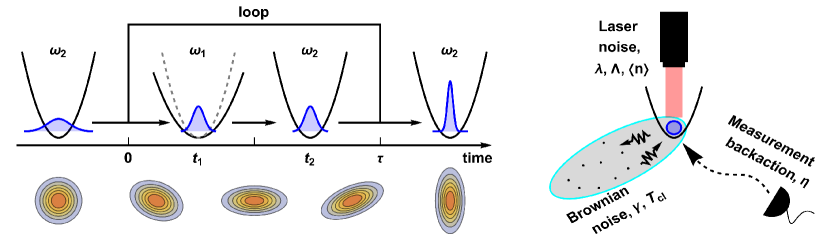
[-0.5cm]a)                                                                                                b)

In this paper, we propose a protocol for the generation of highly squeezed motional states of a massive levitated particle. Our scheme leverages the dynamical switching between two frequencies of a quantum oscillator [46, 47, 48] that has been employed to experimentally generate squeezed states of atomic systems [49]. We apply our protocol to the case of a continuously monitored levitated nanoparticle exposed to collisional, thermal and photon-recoil noise. We show that high levels of squeezing are achievable within a range of parameters compatible with current state-of-the-art setups. We also demonstrate the role of continuous monitoring in achieving squashed states and its apparent immateriality for the task of generating genuinely squeezed ones. Our analysis also allows to establish the conditions that need to be achieved in order to quench the disrupting effects of the open dynamics.

The remainder of the paper is structured as follows. In Sec. I we introduce the protocol for dynamical squeezing, including the implications of a continuous-measurement approach. The solution of the dynamics is given in Sec. II, where we discuss the role that each of the experimental parameters has for the protocol efficiency. Finally, in Sec. III we discuss the experimental feasibility of our protocol and its potential implementation in realistic experimental settings. Sec. IV offers our concluding remarks and future perspectives.

I The squeezing protocol in open system dynamics

The squeezing protocol – The energy of the centre-of-mass motion of a nanoparticle trapped in a time-dependent quadratic optical potential is

$$\hat{H}_{S}(t)=\frac{\hat{p}^{2}}{2m}+\frac{1}{2}m\omega^{2}(t)\hat{x}^{2},$$ (1)

where $\hat{x}$ and $\hat{p}$ are the position and momentum operators of the quantum harmonic oscillator (QHO), $m$ is its mass, and $\omega(t)$ the trap frequency. The squeezing protocol is performed by switching between two frequencies, $\omega_{1}$ and $\omega_{2}$, each being kept constant for a time interval $t_{1}$ and $t_{2}$ respectively [46]. Assuming $\omega_{1}<\omega_{2}$, the control protocol reads

$$\omega(t)=\begin{cases}\omega_{1},\quad 0+n\tau\leq t<t_{1}+n\tau,\\ \omega_{2},\quad t_{1}+n\tau\leq t<t_{1}+t_{2}+n\tau\end{cases}$$ (2)

with $t_{i}=\pi/2\omega_{i}~{}(i=1,2)$, $\tau=t_{1}+t_{2}$ and $n$ labelling the number of squeezing cycles. We assume the system is initially prepared in the quadratic potential with $\omega(t)=\omega_{2}$. The effect of the squeezing protocol is illustrated in Fig. 1a) and detailed in Apd. A. In particular, the squeezing amplitude after $N$ cycles is approximately $r=N\ln(\omega_{1}/\omega_{2})/2$. Needless to say, such growth will not continue indefinitely, and the system variance will eventually stabilise due to the decoherence processes that we now address.

Open dynamics under continuous measurement – In a levitated nanoparticle experiment, the system is optically trapped by a laser and placed in a cold vacuum chamber. The levitated particle interacts with both the laser and the residual gas of the vacuum chamber, resulting in an open system dynamics, which therefore impacts the performance of the squeezing protocol. In particular, we consider the following dissipators [cf. Fig. 1b)]

$$D_{\text{cl}}[\hat{\rho}] =-\frac{i\gamma}{2\hbar}[\hat{x},\{\hat{p},\hat{\rho}\}]-\frac{\gamma mk_{B}T_{\text{cl}}}{\hbar^{2}}[\hat{x},[\hat{x},\hat{\rho}]]-\frac{\gamma}{16mk_{B}T_{\text{cl}}}[\hat{p},[\hat{p},\hat{\rho}]],$$ (3a)

$$D_{\text{th}}[\hat{\rho}] =\frac{i\lambda}{4\hbar}\left([\hat{p},\{\hat{x},\hat{\rho}\}]-[\hat{x},\{\hat{p},\hat{\rho}\}]\right)-\frac{\lambda(2\overline{n}+1)}{4\hbar m\omega}\left(m^{2}\omega^{2}[\hat{x},[\hat{x},\hat{\rho}]]+[\hat{p},[\hat{p},\hat{\rho}]]\right),$$ (3b)

$$D_{\text{lc}}[\hat{\rho}] =-\Lambda[\hat{x},[\hat{x},\hat{\rho}]],$$ (3c)

where $D_{\text{cl}}$ is the modified Caldeira-Leggett dissipator for the collisional noise that arises from the interaction between the system and surrounding residual gas [50, 51], $D_{\text{th}}$ is the thermalisation dissipator that arises from the interaction between the system and the optical modes from the laser, and $D_{\text{lc}}$ describes the decoherence in position due to photon recoils. Here $\gamma,\lambda,\Lambda>0$ are the respective coupling strengths, $m$ is the mass of the nanoparticle, $T_{\text{cl}}$ is the temperature of the chamber, and $\overline{n}$ is the mean excitation number of the particle.

We assume that the position of the nanoparticle is continuously monitored, thus causing a backaction effect that is accounted for by the localization dissipator

$$D[\hat{\rho}]=\sqrt{2\eta\Lambda}H_{\hat{x}}[\hat{\rho}]\mathrm{d}W,$$ (4)

where $H_{\hat{x}}[\hat{\rho}]=\{\hat{x},\hat{\rho}\}-2\text{Tr}\left[\hat{x}\hat{\rho}\right]$ describes the effect of the continuous position measurement, $\eta$ is the measurement efficiency, and $W$ is a Wiener process. By combining the system dynamics with the dissipators as addressed above, the full master equation reads

$${\mathrm{d}}\hat{\rho}=-\frac{i}{\hbar}[\hat{H}_{S},\hat{\rho}]{\mathrm{d}t}+\sum_{i}D_{\text{i}}[\hat{\rho}]{\mathrm{d}t}+\sqrt{2\eta\Lambda}H_{\hat{x}}[\hat{\rho}]\mathrm{d}W,$$ (5)

where the label $i=\text{cl},\text{th},\text{lc}$ refers to the superoperators in Eq. 3.

Description of the dynamics – The process described in Eq. 5 preserves the Gaussian nature of the input state throughout the time evolution. The evolved state can thus be fully characterised by first and second moments of the quadratures $\hat{x}$ and $\hat{p}$ of the system. We define the mean vector $\bm{r}=(\braket{\hat{x}},\braket{\hat{p}})^{T}$ and the covariance matrix (CM) $\bm{\sigma}$ such that $\sigma_{\bm{r}_{i},\bm{r}_{j}}=\frac{1}{2}\left(\braket{\hat{\bm{r}}_{i}\hat{\bm{r}}_{j}}+\braket{\hat{\bm{r}}_{j}\hat{\bm{r}}_{i}}\right)-\braket{\hat{\bm{r}}_{i}}\braket{\hat{\bm{r}}_{j}}$. The CM of the system satisfies the quantum Riccati equation [52]

$$\dot{\bm{\sigma}}=\bm{A}\bm{\sigma}+\bm{\sigma}\bm{A}^{T}+\bm{D}-\bm{\sigma}\bm{B}\bm{B}^{T}\bm{\sigma}$$ (6)

where we have introduced the drift, diffusion, and backaction matrices

$$\bm{A}=\begin{pmatrix}-a_{1}&1/m\\ -m\omega^{2}&-a_{2}\end{pmatrix},~{}\bm{D}=\begin{pmatrix}d_{1}&0\\ 0&d_{2}\end{pmatrix},~{}\bm{B}=\begin{pmatrix}0&b\\ 0&0\end{pmatrix}$$ (7)

with

$$a_{1} =\frac{1}{2}\lambda,\quad a_{2}=a_{1}+\gamma,\quad b=2\sqrt{2\eta\Lambda},$$ (8a)

$$d_{1} =\frac{\hbar^{2}\gamma}{8k_{B}mT_{\text{cl}}}+\frac{\hbar\lambda}{2m\omega}\left(2\overline{n}+1\right),$$ (8b)

$$d_{2} =2\gamma k_{B}mT_{\text{cl}}+\frac{1}{2}\lambda\hbar m\omega\left(2\overline{n}+1\right)+2\hbar^{2}\Lambda.$$ (8c)

In the drift matrix $\bm{A}$, the off-diagonal terms characterise the QHO system in Eq. 1 given the mass and the trap frequency, while the diagonal terms characterise the damping rates in the mean position and momentum of the system. Characterising the drifting matrix $\bm{A}$, we find the time periods in Eq. 2 need to be modified for the open system dynamics, such that $t_{i}=\pi/2\Omega_{i}$ with $\Omega_{i}=\sqrt{\omega_{i}^{2}-(a_{1}-a_{2})^{2}/4}$. The diagonal terms of the diffusion matrix $\bm{D}$ are determined by the dissipation defined in Eq. 3. The continuous measurement leads to an additional term in the dynamics that is characterised by the matrix $\bm{B}$, which contains the efficiency $\eta$ of the continuous measurement. For $\eta=0$, Eq. 6 reduces to the quantum Langevin equation. The connection between the master equation and the Gaussian formalism is discussed in Apd. B.

II Characteristics of the asymptotic state to the protocol

Before investigating the performance of the squeezing protocol in a realistic experimental setting, we first study the asymptotic state of the squeezing protocol, whose dynamics are governed by Eq. 6 for the cases with and without continuous measurement, respectively. In particular, we denote the position variances for the asymptotic CM without the squeezing protocol $\bm{\sigma}^{L,(R)}_{\infty}$ as $\sigma^{L,(R)}_{xx}$, that with the squeezing protocol $\bm{\sigma}^{L(R),\text{sq}}_{\infty}$ as $\sigma_{xx}^{L(R),\text{sq}}$. The superscript $L$ ($R$) stands for the case without (with) continuous measurement.

Asymptotic state without continuous measurement – Given the initial system CM $\bm{\sigma}_{0}$, the evolved system CM $\bm{\sigma}^{L}_{t}$ for $\eta=0$ is the solution of the quantum Lyapunov equation resulting from setting $B=0$ in Eq. (6). This can be cast as

$$\bm{\sigma}^{L}_{t}=e^{t\bm{A}}(\bm{\sigma}_{0}-\bm{X})e^{t\bm{A}^{T}}+\bm{X},$$ (9a)

where the characteristic matrix $$\bm{X}$$ is the solution to the homogeneous equation

$$\bm{A}\bm{X}+\bm{X}\bm{A}^{T}+\bm{D}=\bm{0}.$$ (9b)

For a time-independent problem with constant drift and diffusion matrices $\bm{A}$ and $\bm{D}$, we have the asymptotic solution

$$\bm{\sigma}^{L}_{t\to\infty}=\bm{X}.$$ (10)

Under the action of the squeezing protocol in Eq. 2, we are led to the time-evolved CM after $n$ squeezing loops

$$\bm{\sigma}^{L,\text{sq}}_{t=n\tau}=(\bm{S}^{L}_{2}\circ\bm{S}^{L}_{1}(\bm{\sigma}_{0}))^{n}$$ (11)

with $\bm{S}^{L}_{i}(\bm{\sigma})=e^{t_{i}\bm{A}_{i}}(\bm{\sigma}-\bm{X}_{i})e^{t_{i}\bm{A}_{i}^{T}}+\bm{X}_{i}~{}(i=1,2)$ describing the squeezing operation when the trap frequency is set to $\omega_{i}$, matrices $\bm{A}_{i}$ and $\bm{X}_{i}$ the drift and characteristic matrices in Eqs. 7 and 9b, and $\circ$ standing for the composition of operations. Based on Eq. 11, the dynamics switches depending on the trap frequency, and corresponding asymptotic state with the squeezing protocol $\bm{\sigma}^{L,\text{sq}}_{\infty}$ can be computed numerically.

Asymptotic state with continuous measurement – The case with continuous measurement is studied in a similar manner as that without it. Given the initial system variance $\bm{\sigma}_{0}$, the evolved system variance $\bm{\sigma}^{R}_{t}$ following the quantum Riccati equation in Eq. 6 can be solved analytically. The solution $\bm{\sigma}^{R}_{t}$ can be obtained via [53]

$$\bm{\delta}_{t}-\bm{{\cal X}}_{2}=e^{-t\bm{{\cal A}}^{T}}(\bm{\delta}_{0}-\bm{{\cal X}}_{2})e^{-t\bm{{\cal A}}},$$ (12)

where we define $\bm{\delta}_{t}=(\bm{\sigma}^{R}_{t}-\bm{{\cal X}}_{1})^{-1}$, $\bm{{\cal A}}=\bm{A}-\bm{{\cal X}}_{1}\bm{B}\bm{B}^{T}$. The characteristic matrices $\bm{{\cal X}}_{1}$ and $\bm{{\cal X}}_{2}$ satisfy the conditions

$$\bm{A}\bm{{\cal X}}_{1}+\bm{{\cal X}}_{1}\bm{A}^{T}+\bm{D}-\bm{{\cal X}}_{1}\bm{B}\bm{B}^{T}\bm{{\cal X}}_{1}=\bm{0},$$ (13)

$$\bm{{\cal A}}^{T}\bm{{\cal X}}_{2}+\bm{{\cal X}}_{2}\bm{{\cal A}}-\bm{B}\bm{B}^{T}=\bm{0}.$$

The derivation of such solution is shown in Apd. C. For a time-independent QHO system with fixed matrices $\bm{A}$, $\bm{D}$ and $\bm{B}$, the system variance govern by Eq. 12 converges at $t\to\infty$, such that

$$\bm{\sigma}^{R}_{t\to\infty}=\bm{{\cal X}}_{1}+\bm{{\cal X}}_{2}^{-1}.$$ (14)

When the squeezing protocol is performed, the dynamics of the system variance is characterised by an expression similar to Eq. 11, namely

$$\bm{\sigma}^{R,\text{sq}}_{t=n\tau}=(\bm{S}^{R}_{2}\circ\bm{S}^{R}_{1}(\bm{\sigma}_{0}))^{n},$$ (15)

where the squeezing processes $\bm{S}^{R}_{1,2}$ are given by Eq. 12 for the respective frequency $\omega_{1,2}$. The corresponding asymptotic state (which we compute numerically) is denoted as $\bm{\sigma}^{R,\text{sq}}_{\infty}$.

Features of the asymptotic states – The squeezing process described by Eq. 11 may cause an unstable asymptotic state due to the explosive expansion of one quadrature during the squeezing of the other quadrature. This issue can be circumvented by applying continuous measurement along with the squeezing protocol as the dynamics described by Eq. 15. Indeed, suppose the variance of a system’s quadrature $\sigma_{n}$ follows the relation $\sigma_{n+1}=e^{sr}\sigma_{n}+\chi$ at $n$-th squeezing cycle, where ${sr}$ is the squeezing parameter and $\chi>0$ is the amount of diffusion over one squeezing cycle. The quadrature variance $\sigma_{\infty}$ approaches to a steady point ${\chi}/{(1-e^{sr})}$ if $sr<0$ and to the infinity if $sr\geq 0$. Experimentally, the infinity variance means that the system can become unstable after a number of squeezing cycles, when one quadrature of the system expands too much to be well contained by the trap.

We demonstrate this issue with the system’s momentum variance, when the system is squeezed in its position. Without applying the continuous measurement, Eq. 11 gives the squeezing parameters for each term in the CM, where the momentum one reads

$${sr}_{pp}\approx-\frac{\pi(a_{1}+a_{2})(\Omega_{1}+\Omega_{2})}{2\Omega_{1}\Omega_{2}}+\ln\left(\frac{\Omega_{2}^{2}}{\Omega_{1}^{2}}+O(\Delta a)\right),$$ (16)

with $\Delta a=a_{2}-a_{1}>0$ and $\Omega_{i}=\sqrt{\omega_{i}^{2}-(a_{1}-a_{2})^{2}/4}$. The full expressions for all squeezing parameters are given in Apd. D. Given the definition $\omega_{1}<\omega_{2}$ (hence $\Omega_{1}<\Omega_{2}$), and the small damping regime $\Delta a\to 0$, we notice it is possible to have ${sr}_{pp}>0$ when the damping rate $a_{1}$ is small, while the other two parameters ${sr}_{xx}$ and ${sr}_{xp}$ remain negative for any setting of $\Omega_{1,2}$ and $a_{1,2}$, as illustrated by Fig. 2a). This leads to the explosion of the system momentum variance (whose asymptotic value goes to infinity) in the regime of high quality factors $Q\sim\omega_{2}/a_{1}$. This issue can be circumvented when the continuous measurement is applied to the system, as shown by the open and filled diamonds in Fig. 2b), representing the cases without and with continuous measurement ($b=2$), respectively. Therefore, we conclude that continuous measurement is crucial for applying the squeezing protocol in the high-quality regime, since it guarantees that the system under the squeezing protocol will always reach a stable state with a finite position and momentum variances.

(a))

(b))

Figure 2: Analysis of the asymptotic states. Panel a) shows the squeezing rates given by Eq. 16 against the damping rate $a_{1}$. Here we set $2\omega_{1}=\omega_{2}=3\pi/2$, $m=a_{2}=1$ and $d_{1}=d_{2}=2$, from which we compute $a_{1}\approx 0.39$. Panel b) shows the asymptotic momentum variance without continuous measurement (open diamonds, computed from Eq. 11) and with continuous measurement (filled diamonds, $b=2$, computed from Eq. 15).

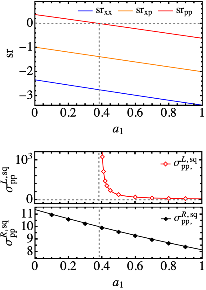
[-5.4cm][-5.4cm]a)b)

(a))

(b))

(c))

Figure 3: Investigation on the position variances for the asymptotic states and the capability of the squeezing protocol given different experimental settings. Panel a) shows the asymptotic position variance without the squeezing protocol against the trap frequency $\omega$ in Eq. 1. The solid line represents the position variance $\sigma^{L}_{xx}$ of Eq. 10 for the case without continuous measurement ($b=0$), in comparison to the position variance $\sigma^{R}_{xx}$ of Eq. 14 for the cases with different measurement strengths ($b=1,3,5$). The reference lines are $\sigma^{L}_{xx}$ with frequency $\omega\to\infty$ and the ground state variance at frequency $\omega_{2}$, i.e. $\sigma^{g}_{xx}=1/3\pi$. Panel b) demonstrates the dynamics of the system position variance when the squeezing protocol is performed. Starting from an arbitrary state, the system position variance equilibrates to $X_{xx}^{\omega_{2}}$ at the time $t=4$. Then, the squeezing protocols without continuous measurement ($\bm{\sigma}^{L,\text{sq}}_{t}$, solid gray line) and with continuous measurement ($\bm{\sigma}^{R,\text{sq}}_{t}$, dashed gray line, $b=3$) are applied. Here, we say that the system is squashed if $\sigma^{g}_{xx}<\sigma^{L(R),\text{sq}}_{xx}<X_{xx}^{\omega_{2}}$, and that it is squeezed if $\sigma^{L(R),\text{sq}}_{xx}<\sigma^{g}_{xx}$. Panel c) shows the ratio between the variances for the squeezed asymptotic state and the ground state, i.e. $\sigma^{L(R),\text{sq}}_{xx}/\sigma^{g}_{xx}$, given different values of $a$, $d$ and $b$. Here the blue region represents for the settings that only achieve squashing, while the red region represents for the settings that achieve squeezing. The borders between two regions (i.e. when $\sigma^{L(R),\text{sq}}_{xx}=\sigma^{g}_{xx}$) are indicated by the black dotted line ($b=0$) and gray dashed lines ($b=3,5$) in the panel.

[-0.3cm]a)                                               b)                                               c)

Features of the squeezing protocol – We show the behaviors of the position variances of the asymptotic states with and without the squeezing protocol and the continuous measurement in Fig. 3c). For the demonstration, we take the parameters $\hbar=m=a_{1,2}=1$, $d_{1,2}=0.5$ and $b=1,3,5$ for the matrices $\bm{A}$, $\bm{D}$, $\bm{B}$ given by Eq. 8.

We first compute the position variance $\sigma^{L}_{xx}$ of the initial state, which changes given different fixed tray frequency $\omega$ (this is the frequency $\omega$ appearing in the Eq. 1), as shown by the solid blue line in Fig. 3a). Here, two black reference lines are given: the first one (dot-dashed line) represents the ground state position variance $\sigma^{g}_{xx}={\hbar}/{(2m\omega_{2})}=1/3\pi$ at frequency $\omega_{2}=3\pi/2$. The second shows the position variance for an infinitely large frequency, $X_{xx}^{\infty}=d_{1}/2(a_{1}+a_{2})$ (dotted line). Clearly, the larger the trap frequency, the smaller the asymptotic state position variance. However, it is not possible to achieve a value of $X_{xx}^{\infty}$ below the ground state position variance $\sigma^{g}_{xx}$. On the other hand, the same relation for the asymptotic state position variances under continuous measurement $\sigma^{R}_{xx}$ are shown with blue dashed lines with strength $b=1,3,5$. Comparing with the case without continuous measurement ($\sigma^{L}_{xx}$, blue solid line), the cases with continuous measurement show that a stronger continuous measurement reduces the position variance of the system. One can have a genuinely squeezed state (with a variance below that of the ground state, $\sigma_{xx}^{R}\leq\sigma^{g}_{xx}$) with a strong continuous measurement (e.g. $b=5$).

To demonstrate the performance of the squeezing protocol, we show the dynamics of the position variance of the system in Fig. 3b). We take two trap frequencies $\omega_{1}=3\pi/4$ and $\omega_{2}=3\pi/2$, such that $\omega_{1}/\omega_{2}=1/2$ and the time for one squeezing loop is $t_{1}+t_{2}=1$. Here, the continuous gray line represents the case without continuous measurement, and the gray dashed line represents the case with continuous measurement ($b=3$). For both scenarios, the system starts from an arbitrary initial state and evolves with trap frequency $\omega_{2}$ with no squeezing protocol applied until it reaches the asymptotic state $X_{xx}^{\omega_{2}}$, which occurs already at $t=4$. Then, the squeezing protocol is applied to the system with and without continuous measurement, respectively. As we can see in our model, we can achieve good degrees of quantum squeezing for both scenarios, leading to the position variances being much smaller than the ground state one, $\sigma_{xx}^{R,\text{sq}}<\sigma_{xx}^{L,\text{sq}}<\sigma^{g}_{xx}$. Moreover, when continuous measurement is performed, we find the overall amplitude of the oscillation of the system is smaller than that without the continuous measurement. This could be advantageous as it suggests that in this case the system remains localised in a smaller region.

The capability of the squeezing protocol given different settings is shown in Fig. 3c), where we show the ratio between the position variances for the asymptotic state and the ground state $\sigma^{L,\text{sq}}_{xx}/\sigma^{g}_{xx}$ under different environmental settings (we take $a_{1}=a_{2}=a$ and $d_{1}=d_{2}=d$). For the values of the parameters in the blue region, the protocol can only squash the system. Conversely, for those in the red region, the protocol can squeeze the system below the ground state variance. The border between the blue and red regions is indicated by the black dotted line, on which one has $\sigma^{L,\text{sq}}_{xx}=\sigma^{g}_{xx}$. The continuous measurement can improve the squeezing over all environmental settings, as indicated by the border of $\sigma_{xx}^{R,\text{sq}}=\sigma^{g}_{xx}$ (dashed lines, $b=3$ and $b=5$) moving towards the blue region as the value of $b$ increases.

III Testing in experimental settings

$m$	$\omega/2\pi$	$\gamma$	$\lambda$	$\Lambda$	$T_{\text{cl}}$	$\overline{n}$	$\eta$
($\mathrm{fg}$)	($\mathrm{kHz}$)	($\mathrm{Hz}$)	($\mathrm{Hz}$)	($\mathrm{m}^{-2}\mathrm{Hz}$)	($\mathrm{K}$)
1	$50\sim 100$	$\geq 10^{-7}$		$10^{23}\sim 10^{26}$	$50$	$10^{7}$	$\leq 0.3$

TAB. 1: Collection of the experimental parameters and their values for the discussion in Sec. III. The connection of the parameter to the respective environment noise is illustrated in Fig. 1b).

To infer the capability of our squeezing protocol in a real experiment, we substitute the parameters in Eq. 7 with those of recent experiments [44, 45, 54, 55, 56, 57, 58]. As a reference, we consider the following setting. Suppose a silica nanoparticle of radius $R=50$ $\mathrm{nm}$ and mass $1$ $\mathrm{fg}$ ($\rho=2200$ $\mathrm{k}\mathrm{g}\mathrm{/}\mathrm{m}^{3}\mathrm{)}$ is levitated in an optical trap, which can oscillate between two frequencies $\omega_{1}/2\pi=50$ $\mathrm{kHz}$ and $\omega_{2}/2\pi=100$ $\mathrm{kHz}$. The experiment is performed in a cryostat and ultra-high-vacuum environment, such that the environment temperature $T_{\text{cl}}=50$ $\mathrm{K}$, and the quality factor $Q=\omega/\gamma$ can be as high as $10^{10}$ [58]. Thus, the damping rates (from the collisional and thermal noises) are weak and they can be estimated by $\gamma\sim\lambda\sim 10^{3}(P/$\mathrm{mbar}$)~{}$\mathrm{Hz}$$, where we assume that the chamber pressure can go as low as $P\geq 10^{-10}$ $\mathrm{mbar}$ [58]. The photon-recoil rate can be estimated by the equation [59, 60, 61]

$$\Lambda=\frac{7\pi\varepsilon_{0}}{30\hbar}\left(\frac{\epsilon_{c}VE_{t}}{2\pi}\right)^{2}k_{0}^{5},$$ (17)

where $\varepsilon_{0}$ is the vacuum permittivity, $\epsilon_{c}=3{(\varepsilon-1)}/{(\varepsilon+2)}$ is written in terms of the the relative dielectric constant $\varepsilon$ of the nanoparticle, whose volume is $V$, $k_{0}=\omega_{0}/c$ with $c$ the speed of light and $\omega_{0}={2\pi c}/{\lambda}$ the laser beam frequency. Following the analysis in Apd. E, we estimate $\Lambda\sim 10^{26}$ $\mathrm{m}^{-2}\mathrm{Hz}$ [62, 61, 63]. We take the mean occupation number of the particle at temperature $50$ $\mathrm{K}$ to be $\overline{n}=10^{7}$. However, the occupation number can be further reduced to $\sim 0.5$ with specific cooling techniques [64], which further reduce the effect of the thermal noise. We estimate that the efficiency of the measurement is no more than $30\%$ [65], and summarise these values in Tab. 1.

(a))

(b))

Figure 4: Contributions of the noises and the squeezing ratio against the quality factor. Panel a) shows the noise contributions from Eq. 18, which rise from the collisional noise ($d_{2}^{\gamma}$), the thermal noise ($d_{2}^{\lambda}$) and the photon-recoil noise ($d_{2}^{\Lambda}$). Panel b) shows the logarithmic relation of the squeezing ratio $\zeta_{\text{sq}}=\sqrt{\sigma_{xx}^{\text{sq}}(\tau)/\sigma_{xx}^{g}}$ against the quality factor $Q=\omega/\gamma(\lambda)$. The blue (red dashed) line represents the cases for $\Lambda=10^{26}$ ($10^{23}$) $\mathrm{m}^{-2}\mathrm{Hz}$, and the square (triangle) represents the corresponding case with $\eta=0.3$.

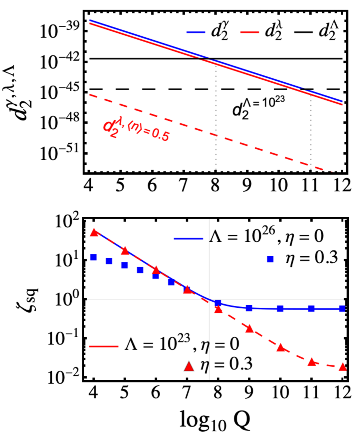
[-4.8cm][-4.8cm]a)b)

We first investigate the contributions of the noises given the setting discussed above. In particular, we scrutinize $d_{2}$ in Eq. 7 and compare the order of magnitudes for each terms. We find the following values (in unit $\mathrm{m}^{2}\mathrm{k}\mathrm{g}^{2}\mathrm{Hz}^{3}$)

$$d_{2}^{\gamma} =2\gamma k_{B}mT_{\text{cl}}\sim 10^{-45},$$ (18a)

$$d_{2}^{\lambda} =\overline{n}\lambda\hbar m\omega\sim 10^{-46},$$ (18b)

$$d_{2}^{\Lambda} =2\hbar^{2}\Lambda\sim 10^{-42},$$ (18c)

where we have taken $\gamma=\lambda=10^{-6}$ $\mathrm{Hz}$, $\Lambda=10^{26}$ $\mathrm{m}^{-2}\mathrm{Hz}$, and $\overline{n}=10^{7}$. This suggests that the strength of collisional and thermal noises are comparable at $T_{\text{cl}}=50$ $\mathrm{K}$, and they can be smaller than the photon-recoil noise for large enough qualify factor $Q$. Indeed, collisional, thermal and photon-recoil noises are comparable when $Q\sim 10^{8}$, as shown by Fig. 4a). On the other hand, if the photon-recoil rate is reduced by $3$ orders, i.e. $\Lambda\sim 10^{23}$ $\mathrm{m}^{-2}\mathrm{Hz}$, collisional and photon-recoil noises are comparable when $Q\sim 10^{11}$.

We then consider the following squeezing experiment [cf. Fig. 3b)]. The levitated particle firstly equilibrates at trap frequency $\omega_{2}$, such that the centre of motion of the particle is a QHO system in the asymptotic state given by Eq. 10. Then, the squeezing protocol is applied to the system at $t=0$, and we measure its position variance at the end of the protocol when $t=\tau$. We denote the position variance of the system at time $t$ to be $\sigma^{\text{sq}}_{xx}(t)$, and take the position variance of the ground state $\sigma^{\text{g}}_{xx}$ at frequency $\omega_{2}$ as the reference. In the best scenario (corresponding to $\gamma=\lambda=10^{-6}$ $\mathrm{Hz}$, $\Lambda=10^{23}$ $\mathrm{m}^{-2}\mathrm{Hz}$, $\overline{n}=10^{7}$), we have

$$\sigma^{\text{sq}}_{xx}(0)=X_{xx}^{\omega_{2}} \approx 3.1\times 10^{-3}\,$\mathrm{n}\mathrm{m}^{2}$,$$ (19a)

$$\sigma^{\text{g}}_{xx}=\frac{\hbar}{2m\omega_{2}} \approx 8.4\times 10^{-5}\,$\mathrm{n}\mathrm{m}^{2}$.$$ (19b)

Hence, the system has an initial position spread being a factor $\zeta_{\text{sq}}(0)=\sqrt{\sigma^{\text{sq}}_{xx}(0)/\sigma^{\text{g}}_{xx}}\sim 10^{4}$ larger than the ground state. In the worst scenario ($\Lambda=10^{26}$ $\mathrm{m}^{-2}\mathrm{Hz}$), such a factor becomes $\zeta^{\prime}_{\text{sq}}(0)\sim 10^{6}$. The capability of the squeezing protocol in a realistic experimental settings is demonstrated by the squeezing ratio $\zeta_{\text{sq}}=\sqrt{\sigma_{xx}^{\text{sq}}(\tau)/\sigma_{xx}^{g}}$ in Fig. 4b), where a value of $\zeta_{\text{sq}}<1$ means the position variance of the system is squeezed below that of the ground state. We consider two cases for the the photon-recoil rate, i.e. $\Lambda=10^{26}$ or $10^{23}$ $\mathrm{m}^{-2}\mathrm{Hz}$, without continuous measurement ($\eta=0$). For small quality factors $Q$, we see that the squeezing ratio $\zeta_{\text{sq}}$ coincides in both cases (blue continuous and red dashed lines), indeed the dynamics is dominated by the collisional and thermal noises. Conversely, we see a plateau (at $Q>10^{8}$ for $\Lambda=10^{26}$ $\mathrm{m}^{-2}\mathrm{Hz}$, and at $Q>10^{11}$ for $\Lambda=10^{23}$ $\mathrm{m}^{-2}\mathrm{Hz}$) when the photon recoils becomes the dominant noise contribution [cf. Fig. 4a)]. In both cases, the squeezing ratio $\zeta_{\text{sq}}$ at high quality factor is below 1, indicating that one can achieve genuine squeezing in a levitation experiment at ultra high vacuum. Based on our model, we have $\zeta_{\text{sq}}\approx 0.58$ at $Q=10^{12}$ for $\Lambda=10^{26}$ $\mathrm{m}^{-2}\mathrm{Hz}$ and $\zeta_{\text{sq}}\approx 0.02$ at $Q=10^{12}$ for $\Lambda=10^{23}$ $\mathrm{m}^{-2}\mathrm{Hz}$.

Squares and triangles in Fig. 4b) represent the cases taking the continuous measurement with $\eta=0.3$, which only provide a small improvement to the squeezing (e.g. $\zeta_{\text{sq}}^{\eta=0.3}\approx 0.57$ at $Q=10^{12}$ for $\Lambda=10^{26}$ $\mathrm{m}^{-2}\mathrm{Hz}$), which cannot be seen using the logarithmic scale. Indeed, the effect of the continuous measurement becomes only prominent when the photon-recoil noise is large ($\Lambda=10^{26}$ $\mathrm{m}^{-2}\mathrm{Hz}$) and the qualify factor is low ($Q<10^{8}$), thus enhancing the squashing effect. If the photon-recoil noise can be reduced (e.g. when $\Lambda=10^{23}$ $\mathrm{m}^{-2}\mathrm{Hz}$), the continuous measurement would not produce any improvement in the squeezing even for the low qualify factor [cf. red line and triangles in the figure]. Indeed, the continuous measurement effect described by Eq. 4 is proportional to the photon-recoil noise $\Lambda$.

IV Conclusions

We have proposed a squeezing protocol (via frequency jumps) applied to a levitated nanoparticle subjected to continuous monitoring of its position. The dynamics of the system is influenced by the collisional, thermal, and photon-recoil noise, and influenced by the stochastic noise caused by the continuous measurement. We have estimated the potential for achieving large squeezing of the considered massive quantum system, considering parameters from recent experiments. We have found that while the photon-recoil noise plays a dominant role, in the high quality-factor regime, the position spread of the system can still be squeezed below the ground state variance. The backaction from continuous measurement does not help squeezing performances. Our study addresses the engineering of genuine quantum resources for sensing and metrology in levitated optomechanics, while also providing a route to the achievement of states that will be crucial for investigations on the foundations of quantum mechanics. The closeness of our assessment to experimental reality paves the way to a ready implementation of the scheme.

Appendix A The squeezing protocol

Squeezing of the motion of a harmonic oscillator through the dynamical switching of frequency has been proposed in Ref. [46, 47, 48], and has been employed to experimentally generate squeezing in atomic systems [49]. This operation is based on the Bogoliubov transformation which describes the effect of switching the frequency of the oscillator. Given the Hamiltonian in Eq. 1, we call $\{\hat{a},\hat{a}^{\dagger}\}$ ($\{\hat{b},\hat{b}^{\dagger}\}$) the ladder operators corresponding to frequency $\omega_{1}$ ($\omega_{2}$). They satisfy the relations

$$\hat{b}=\mu\hat{a}+\nu\hat{a}^{\dagger},\qquad\hat{b}^{\dagger}=\mu\hat{a}^{\dagger}+\nu\hat{a},$$ (20)

where $\mu=\cosh(r)=(\omega_{1}+\omega_{2})/{2\sqrt{\omega_{1}\omega_{2}}}$, $\nu=\sinh(r)=(\omega_{1}-\omega_{2})/{2\sqrt{\omega_{1}\omega_{2}}}$ and $r=\frac{1}{2}\ln(\omega_{2}/\omega_{1})$. The Bogoliubov transformation is linked to the squeezing operation such that $\hat{b}=\hat{S}^{\dagger}(r)\hat{a}\hat{S}(r)$ with

$$\hat{S}(r)=\exp\left[\frac{1}{2}(r\hat{a}^{2}-r\hat{a}^{{\dagger}2})\right].$$ (21)

Therefore, switching the frequency of the oscillator leads to a squeezing operation on the system.

To achieve squeezing in the position of the system, a squeezing protocol is defined by Eq. 2 in the main text, which gives the equations for the expectation values of the quadrature operators $\hat{x}$ and $\hat{p}$ as

$$\frac{\mathrm{d}}{\mathrm{d}t}\braket{\hat{x}} =\frac{\braket{\hat{p}}}{m},$$ (22a)

$$\frac{\mathrm{d}}{\mathrm{d}t}\braket{\hat{p}} =-m\omega^{2}\braket{\hat{x}}.$$ (22b)

Indeed, in each time period $t_{i}$, the dynamics of the quadratures in Eq. 22 can be solved analytically with $\omega=\omega_{i}$. By defining the initial mean position and momentum of the system as $x_{0}=\braket{\hat{x}(0)}$ and $p_{0}=\braket{\hat{p}(0)}$, the evolution results in the transformation $(x_{0},p_{0})^{T}\mapsto\bm{M}_{i}(t)(x_{0},p_{0})^{T}$ with

$$\bm{M}_{i}(t)=\begin{pmatrix}\cos(\omega_{i}t)&\sin(\omega_{i}t)/m\omega_{i}\\ -m\omega_{i}\sin(\omega_{i}t)&\cos(\omega_{i}t)\end{pmatrix}.$$ (23)

This transformation leads to the combined action of rotation and squeezing of the system. In particular, the protocol defined in Eq. 2 acts on the system in the following way [cf. Fig. 1b) where the protocol is illustrated]: when $\omega=\omega_{1}$, the system is squeezed along the $\hat{x}$ quadrature. When $\omega=\omega_{2}$, the system is squeezed along the $\hat{p}$ quadrature. However, after the first part of squeezing $t\geq t_{1}=\pi/2\omega_{1}$, the quadratures of the system swap due to the rotation of the system, $\hat{x}\leftrightarrow\hat{p}$. Therefore, the second part of the protocol acts on the same quadrature as the first part does. After time $\tau$, this gives the transformation of the average values of the quadratures $x_{\tau}=\braket{\hat{x}(\tau)}$ and $p_{\tau}=\braket{\hat{p}(\tau)}$ as

$$(x_{\tau},p_{\tau})^{T} =\bm{M}_{2}(t_{2})\circ\bm{M}_{1}(t_{1})~{}(x_{0},p_{0})^{T}$$ (24)

$$=-\left(e^{r}x_{0},e^{-r}p_{0}\right),$$

where we have defined $e^{r}\equiv\omega_{1}/\omega_{2}$, and the squeezing parameter $r=\ln{\omega_{1}}/{\omega_{2}}$. Eq. 24 results in squeezing of the position quadrature, so that the variance $\sigma_{xx}(0)=\braket{\hat{x}^{2}(0)}$ transforms to

$$\sigma_{xx}(\tau)=e^{2r}\sigma_{xx}(0),$$ (25)

where we set $\braket{\hat{x}(0)}=0$. Thus, a total degree of squeezing $e^{2r}$ is achieved after a time $\tau=\pi/2\omega_{1}+\pi/2\omega_{2}$.

Appendix B Connection between the matrix and the Gaussian formalism

The Gaussian process described by Eq. 5 can be fully characterised by the first and second moments of the quadratures by taking $\mathrm{d}\braket{\hat{O}}=\text{Tr}\left[\hat{O}\,\mathrm{d}\hat{\rho}\right]$ and using the invariance of trace under cyclic permutation of its arguments [66]. Given the definitions $\hat{\bm{r}}=\{\hat{x},\hat{p}\}$ and $\bm{\sigma}_{\bm{r}_{i},\bm{r}_{j}}=\frac{1}{2}\left(\braket{\hat{\bm{r}}_{i}\hat{\bm{r}}_{j}}+\braket{\hat{\bm{r}}_{j}\hat{\bm{r}}_{i}}\right)-\braket{\hat{\bm{r}}_{i}}\braket{\hat{\bm{r}}_{j}}$, we can write the equation for the system variances as

$$\dot{\sigma}_{x,x} =\frac{2}{m}\sigma_{x,p}-\lambda\sigma_{x,x}+\frac{\gamma\hbar^{2}}{8k_{B}mT_{\text{cl}}}+\frac{\lambda\hbar}{2m\omega}(2\overline{n}+1)$$

$$-8\eta\Lambda\sigma^{2}_{x,x},$$ (26a)

$$\dot{\sigma}_{p,p} =-2m\omega^{2}\sigma_{x,p}+(2\gamma-\lambda)\sigma_{p,p}+2\gamma k_{B}mT_{\text{cl}}$$

$$+\frac{1}{2}\lambda\hbar m\omega(2\overline{n}+1)+2\Lambda\hbar^{2}-8\eta\Lambda\sigma^{2}_{x,p},$$ (26b)

$$\dot{\sigma}_{x,p} =\frac{1}{m}\sigma_{p,p}-m\omega^{2}\sigma_{x,x}-(\lambda-\gamma)\sigma_{x,p}-\frac{i\hbar}{2}(\lambda+\gamma)$$

$$-8\eta\Lambda\sigma_{x,x}\sigma_{x,p}.$$ (26c)

The original Riccati equation Eq. 6 reads [52]

$$\dot{\bm{\sigma}} =\tilde{\bm{A}}\bm{\sigma}+\bm{\sigma}\tilde{\bm{A}}^{T}+\tilde{\bm{D}}-\bm{\sigma}\bm{B}\bm{B}^{T}\bm{\sigma},$$ (27a)

where

$$\tilde{\bm{A}} =\bm{B}-\bm{\Omega}\bm{C}\bm{\sigma}_{B}\frac{1}{\bm{\sigma}_{B}+\bm{\sigma}_{M}}\bm{\Omega}\bm{C}^{T},$$ (27b)

$$\tilde{\bm{D}} =\bm{D}+\bm{\Omega}\bm{C}\bm{\sigma}_{B}\frac{1}{\bm{\sigma}_{B}+\bm{\sigma}_{M}}\bm{\sigma}_{B}\bm{C}^{T}\bm{\Omega},$$ (27c)

$$\bm{B} =\bm{C}\bm{\Omega}\sqrt{\frac{1}{\bm{\sigma}_{B}+\bm{\sigma}_{M}}},$$ (27d)

$$\bm{\Omega} =\begin{pmatrix}0&1\\ -1&0\end{pmatrix},\quad\bm{C}=2\sqrt{\Lambda}~{}\begin{pmatrix}1&0\\ 0&0\end{pmatrix},$$ (27e)

with $\bm{A}$ being the drift matrix, $\bm{D}$ the diffusion matrix, $\bm{\Omega}$ the symplectic matrix, $\bm{C}$ the coupling matrix between the system and the light mode, $\bm{\sigma}_{B}$ and $\bm{\sigma}_{M}$ the CMs for the light mode and the measurement, respectively. When the continuous measurement is considered, and assuming no thermal photon, the CM for the light mode is

$$\bm{\sigma}_{B}=\mathds{1}_{2},$$ (28)

where $\mathds{1}_{2}$ is the identity matrix. For a perfectly efficient measurement ($\eta=1$), the CM for the Gaussian measurement reads

$$\bm{\sigma}_{M}=\begin{pmatrix}s&0\\ 0&1/s\end{pmatrix}\bm{\sigma}_{B}.$$ (29)

Here, the factor $s\in(0,\infty)$ characterises the type of the general-dyne detection: the choice $s=1$ ($s\rightarrow\infty$) is for a heterodyne (detection and gives the (homodyne) measurement. For an inefficient Gaussian measurement ($\eta\in]0,1[$), the resulting CM is that of a mixture [52, 67]

$$\bm{\sigma}_{M}^{\ast}=\frac{1}{\eta}\bm{\sigma}_{M}+\frac{1-\eta}{\eta}\bm{\sigma}_{B}.$$ (30)

Considering the homodyne detection, and taking $\bm{\sigma}_{M}^{\ast}$ instead of $\bm{\sigma}_{M}$ in Eq. 6, one has

$$\tilde{\bm{A}}=\bm{A},\quad\tilde{\bm{D}}=\bm{D},\quad\bm{B}=\begin{pmatrix}0&b\\ 0&0\end{pmatrix}$$ (31)

with $b=\sqrt{8\eta\Lambda}$. By comparing Eqs. 6, 26 and 31, one can get the values for $a_{1},a_{2},d_{1},d_{2},b$ in Eq. 7 that link Eq. 6 to the stochastic master equation Eq. 5 in the main text. This reduces to the Langevin equation in Eq. 6 for $\eta=0$.

Appendix C Investigation on the squeezing protocol in open dynamics

Here we derive the solution of Eq. 6 following the method in Ref. [53, 68].

Quantum Langevin equation – For $\eta=0$, Eq. 6 can be transformed to a first-order linear differential equation

$$\frac{\mathrm{d}}{\mathrm{d}t}\begin{pmatrix}\bm{N}_{t}\\ \bm{\Psi}_{t}\end{pmatrix}=\bm{\mathcal{H}}\begin{pmatrix}\bm{N}_{t}\\ \bm{\Psi}_{t}\end{pmatrix},\text{ with }\bm{\mathcal{H}}=\begin{pmatrix}-\bm{A}^{T}&\bm{0}\\ \bm{D}&\bm{A}\end{pmatrix},$$ (32)

where we introduce

$$\bm{\Psi}_{t}=\bm{\sigma}_{t}\bm{N}_{t},\quad\text{and}\quad\dot{\bm{N}}_{t}=-\bm{A}^{T}\bm{N}_{t},$$ (33)

and let $\bm{N}_{0}$ to be the identity matrix $\bm{\mathds{1}}$. The linear different equation given by Eq. 32 can be solved by making the matrix $\bm{\mathcal{H}}$ diagonal. Consider the similarity transformation

$$\bm{T}=\begin{pmatrix}\mathds{1}&\bm{0}\\ \bm{X}&\mathds{1}\end{pmatrix},$$ (34)

such that $\bm{T}\bm{T}^{-1}=\bm{T}^{-1}\bm{T}=\mathds{1}$, and define $\bm{X}$ as the solution to the equation

$$\bm{A}\bm{X}+\bm{X}\bm{A}^{T}+\bm{D}=\bm{0}.$$ (35)

Apply the transformation on $\bm{\mathcal{H}}$, such that

$$\tilde{\bm{\mathcal{H}}}\equiv\bm{T}^{-1}{\bm{\mathcal{H}}}\bm{T}=\begin{pmatrix}-\bm{A}^{T}&\bm{0}\\ \bm{0}&\bm{A}\end{pmatrix}.$$ (36)

where the transformed matrix $\bm{\mathcal{H}}$ becomes diagonal. Correspondingly, Eq. 32 is transformed to

$$\frac{\mathrm{d}}{\mathrm{d}t}\begin{pmatrix}\tilde{\bm{N}}_{t}\\ \tilde{\bm{\Psi}}_{t}\end{pmatrix}=\tilde{\bm{\mathcal{H}}}\begin{pmatrix}\tilde{\bm{N}}_{t}\\ \tilde{\bm{\Psi}}_{t}\end{pmatrix},$$ (37)

with the transformed vector defined as

$$\begin{pmatrix}\tilde{\bm{N}}_{t}\\ \tilde{\bm{\Psi}}_{t}\end{pmatrix}\equiv\bm{T}^{-1}\begin{pmatrix}\bm{N}_{t}\\ \bm{\Psi}_{t}\end{pmatrix}=\begin{pmatrix}\bm{N}_{t}\\ \bm{\Psi}_{t}-\bm{X}\bm{N}_{t}\end{pmatrix}.$$ (38)

The transformed differential equation has the solution

$$\begin{pmatrix}\tilde{\bm{N}}_{t}\\ \tilde{\bm{\Psi}}_{t}\end{pmatrix}=e^{t\tilde{\bm{\mathcal{H}}}}\begin{pmatrix}\tilde{\bm{N}}_{0}\\ \tilde{\bm{\Psi}}_{0}\end{pmatrix},$$ (39)

which in details reads

$$\bm{N}_{t} =\tilde{\bm{N}}_{t}=e^{-t\bm{A}^{T}}\tilde{\bm{N}}_{0}=e^{-t\bm{A}^{T}}\bm{X}_{0}=e^{-t\bm{A}^{T}},$$ (40)

$$\bm{\Psi}_{t} -\bm{X}\bm{N}_{t}=\tilde{\bm{\Psi}}_{t}=e^{t\bm{A}}\tilde{\bm{\Psi}}_{0}=e^{t\bm{A}}(\bm{\sigma}_{0}-\bm{X}).$$

By applying Eq. 33 to Eq. 40, one can get the solution to the CM for the system $\bm{\sigma}_{t}$ as in Eq. 9 for the quantum Langevin equation. If the squeezing protocol is not performed, i.e. a time-independent QHO with constant drifting and diffusion matrices $\bm{A}$ and $\bm{D}$, the asymptotic state for Eq. 9 can be easily shown to be the characteristic matrix $\bm{X}$ given by Eq. 35, such that $\bm{\sigma}_{t\to\infty}=\bm{X}$.

One can attempt to find the asymptotic state of the squeezing dynamics described by Eq. 11. By introducing $\Delta\bm{X}=\bm{X}_{1}-\bm{X}_{2}$ and $\bm{\alpha}$ satisfying

$$\bm{\alpha}-e^{t_{2}\bm{A}_{2}}e^{t_{1}\bm{A}_{1}}\bm{\alpha}e^{t_{1}\bm{A}_{1}^{T}}e^{t_{2}\bm{A}_{2}^{T}}=\Delta\bm{X}-e^{t_{2}\bm{A}_{2}}\Delta\bm{X}e^{t_{2}\bm{A}_{2}^{T}},$$ (41)

the CM for one round of squeezing, i.e. at time $\tau=t_{1}+t_{2}$, results from

$$\bm{\sigma}_{\tau}-\bm{X}_{1}+\bm{\alpha}=e^{t_{2}\bm{A}_{2}}e^{t_{1}\bm{A}_{1}}(\bm{\sigma}_{0}-\bm{X}_{1}+\bm{\alpha})e^{t_{1}\bm{A}_{1}^{T}}e^{t_{2}\bm{A}_{2}^{T}},$$ (42)

and the asymptotic state is given by $\bm{\sigma}^{\text{sq}}_{t\to\infty}=\bm{X}_{1}-\bm{\alpha}$.

Quantum Riccati equation – A similar transformation can be done introducing

$$\bm{\Psi}_{t}=\bm{\sigma}_{t}\bm{N}_{t},\quad\text{and}\quad\dot{\bm{N}}_{t}=-\bm{A}^{T}\bm{N}_{t}+\bm{B}\bm{B}^{T}\bm{\sigma}_{t}\bm{N}_{t},$$ (43)

such that one has

$$\frac{\mathrm{d}}{\mathrm{d}t}\begin{pmatrix}N_{t}\\ \Psi_{t}\end{pmatrix}=\mathcal{H}\begin{pmatrix}N_{t}\\ \Psi_{t}\end{pmatrix},\text{ with }\mathcal{H}=\begin{pmatrix}-A^{T}&BB^{T}\\ D&A\end{pmatrix},$$ (44)

and $\bm{N}_{0}$ is given by the identity matrix. Introduce two similarity transformations,

$$\bm{T}_{1}=\begin{pmatrix}\mathds{1}&\bm{0}\\ \bm{{\cal X}}_{1}&\mathds{1}\end{pmatrix},\quad\bm{T}_{2}=\begin{pmatrix}\mathds{1}&\bm{{\cal X}}_{2}\\ \bm{0}&\mathds{1}\end{pmatrix},$$ (45)

and letting $\bm{{\cal X}}_{1}$ and $\bm{{\cal X}}_{2}$ be the solutions to the equations

$$\bm{A}\bm{{\cal X}}_{1}+\bm{{\cal X}}_{1}\bm{A}^{T}+\bm{D}-\bm{{\cal X}}_{1}\bm{B}\bm{B}^{T}\bm{{\cal X}}_{1}=\bm{0},$$ (46a)

$$\bm{{\cal A}}^{T}\bm{{\cal X}}_{2}+\bm{{\cal X}}_{2}\bm{{\cal A}}-\bm{B}\bm{B}^{T}=\bm{0},$$ (46b)

the characterisation matrix is diagonalised such that

$$\bm{\mathcal{H}}^{\prime\prime}=\bm{T}_{2}^{-1}\bm{T}_{1}^{-1}\bm{{\cal H}}\bm{T}_{1}\bm{T}_{2}=\begin{pmatrix}-\bm{{\cal A}}^{T}&\bm{0}\\ \bm{0}&\bm{{\cal A}}\end{pmatrix},$$ (47)

where we define $\bm{{\cal A}}=\bm{A}-\bm{{\cal X}}_{1}\bm{B}\bm{B}^{T}$. Define the transformed vector

$$\begin{pmatrix}\bm{N}^{\prime\prime}_{t}\\ \bm{\Psi}^{\prime\prime}_{t}\end{pmatrix} \equiv\bm{T}_{2}^{-1}\bm{T}_{1}^{-1}\begin{pmatrix}\bm{N}_{t}\\ \bm{\Psi}_{t}\end{pmatrix}$$ (48)

$$=\begin{pmatrix}\bm{N}_{t}+\bm{{\cal X}}_{2}\bm{{\cal X}}_{1}\bm{N}_{t}-\bm{{\cal X}}_{2}\bm{\Psi}_{t}\\ \bm{\Psi}_{t}-\bm{{\cal X}}_{1}\bm{N}_{t}\end{pmatrix},$$ (49)

The differential equation in Eq. 44 can be solved as

$$\begin{pmatrix}\bm{N}^{\prime\prime}_{t}\\ \bm{\Psi}^{\prime\prime}_{t}\end{pmatrix}=e^{t\bm{\mathcal{H}}^{\prime\prime}}\begin{pmatrix}\bm{N}^{\prime\prime}_{0}\\ \bm{\Psi}^{\prime\prime}_{0}\end{pmatrix},$$ (50)

and the solution on the CM for the system is then given by

$$(\bm{\sigma}_{t}-\bm{{\cal X}}_{1})\bm{\xi}_{t}^{-1}=e^{t\bm{{\cal A}}}(\bm{\sigma}_{0}-\bm{{\cal X}}_{1})\bm{\xi}_{0}^{-1}e^{t\bm{{\cal A}}^{T}},$$ (51)

where we take $\bm{\xi}_{t}=\mathds{1}-\bm{{\cal X}}_{2}(\bm{\sigma}_{t}-\bm{{\cal X}}_{1})$. Take the inverse of Eq. 51 and define $\bm{\delta}_{t}=(\bm{\sigma}_{t}-\bm{{\cal X}}_{1})^{-1}$, the solution gives Eq. 12 in the main text.

The asymptotic state of Eq. 12 without the squeezing protocol reads $\bm{\sigma}_{t\to\infty}=\bm{X}_{1}+\bm{X}_{2}^{-1}$. The asymptotic state with the squeezing protocol is however difficult to attain, therefore we take the numerical solution instead.

Appendix D The squeezing protocol

Suppose the quadrature variance follows the relation $\sigma_{n+1}=e^{sr}\sigma_{n}+\chi$ after one squeezing process, which can be recast into the form

$$\sigma_{n+1}-\frac{\chi}{1-e^{sr}}=e^{sr}\left(\sigma_{n}-\frac{\chi}{1-e^{sr}}\right).$$ (52)

One can see that, for a finite $\chi>0$, this dynamics leads the variance to a steady positive value $\sigma_{\infty}\to\frac{\chi}{1-e^{sr}}$ when ${sr}<0$, or to the infinity $\sigma_{\infty}\to\infty$ when ${sr}>0$. The squeezing parameters in our protocol can be acquired by setting the diffusion to be zero in Eq. 11 ($d_{1,2}\to 0$ leads to $\chi\to 0$ while leaving $e^{sr}$ unchanged), which read

$${sr}_{xx} =f+\ln\left({\Omega_{1}^{2}}/{\Omega_{2}^{2}}\right),$$ (53)

$${sr}_{pp} =f+\ln\left(\frac{\Omega_{2}^{2}}{\Omega_{1}^{2}}+\Delta a\frac{m(\Omega_{2}^{2}-\Omega_{1}^{2})}{\Omega_{1}^{2}}\frac{\sigma_{xp,n}}{\sigma_{pp,n}}\right.$$

$$~{}~{}~{}~{}~{}~{}~{}~{}+\left.\Delta a^{2}\frac{m^{2}(\Omega_{2}^{2}-\Omega_{1}^{2})^{2}}{4\Omega_{1}^{2}\Omega_{2}^{2}}\frac{\sigma_{xx,n}}{\sigma_{pp,n}}\right),$$ (54)

$${sr}_{xp} =f+\ln\left(1+\Delta a\frac{m(\Omega_{2}^{2}-\Omega_{1}^{2})}{2\Omega_{2}^{2}}\frac{\sigma_{xx,n}}{\sigma_{xp,n}}\right),$$ (55)

where $f={\pi(a_{1}+a_{2})(\Omega_{1}+\Omega_{2})}/{(2\Omega_{1}\Omega_{2})}$ and $\Delta a=a_{2}-a_{1}$. In the limit of $\Delta a\to 0$, this gives Eq. 16.

Appendix E Range of coefficients

Pars (unit)	Values	Pars (unit)	Values
$R$ ($\mathrm{nm}$)	50	$\lambda$ ($\mathrm{nm}$)	$1550$
$P_{t}$ ($\mathrm{W}$)	0.50	$W_{t}$ ($\mathrm{nm}$)	$1000$
$\varepsilon_{0}$ ($\mathrm{F}\mathrm{/}\mathrm{n}\mathrm{m}$)	$8.9\times 10^{-21}$	$\epsilon$	$2$
$A_{x}$	$1$	$A_{y}$	$0.9$

TAB. 2: Collection of the experimental parameters and their values for the computation of the photon-recoil rate.

The dissipation due to gas is described by Eq. 3a where $T$ is the temperature of the chamber and $\gamma$ is the viscous friction that can be calculated from kinetic gas theory [69, 70]:

$$\gamma=\frac{64}{3}\frac{R^{2}P}{mv_{\mathrm{gas}}}\sim 10^{3}(P/$\mathrm{mbar}$)~{}$\mathrm{Hz}$.$$ (56)

with the mean gas velocity $v_{\mathrm{gas}}=\sqrt{8k_{b}T_{\text{cl}}/(\pi m_{\mathrm{gas}})}$, and $m_{\mathrm{gas}}\approx 10^{-24}\,$\mathrm{kg}$$ is the average of the gas molecules. $R$ is the radius of the nanoparticle and $P$ is the pressure in the vacuum chamber. Our estimation has been achieved in the latest experiment [58]. The thermal dissipation due to energy exchange with the laser is described by Eq. 3b, where the coupling rate is estimated by $\lambda\sim\gamma$ as they contribute equally to the damping rate in momentum, i.e. $a_{2}\approx\lambda+\gamma$. We set $\overline{n}=(\exp(\hbar\omega/k_{b}T)-1))^{-1}\sim 10^{7}$ as the mean occupation of the nanoparticle at $\omega/2\pi=100$ $\mathrm{kHz}$ and $T=50$ $\mathrm{K}$. This gives the estimation of the thermalisation rate such that

$$\lambda\overline{n}\sim 10^{8}(P/$\mathrm{mbar}$)~{}$\mathrm{Hz}$.$$ (57)

The position detection due to the measurements of the photons scattered back from the nanoparticle is described by Eq. 3c, where the coupling strengths reads [59, 61, 60]

$$\Lambda=\frac{7\pi\varepsilon_{0}}{30\hbar}\left(\frac{\epsilon_{c}VE_{t}}{2\pi}\right)^{2}k_{0}^{5}\sim 7\times 10^{25}~{}($\mathrm{m}^{-2}\mathrm{Hz}$),$$ (58)

where $\varepsilon_{0}$ is the vacuum permittivity, $\epsilon_{c}=3{(\varepsilon-1)}/{(\varepsilon+2)}$, and $\epsilon$ is the relative dielectric constant of the nanoparticle. $V$ is the volume of the nanoparticle, $k_{0}=\omega_{0}/c$ with $c$ being the speed of light and $\omega_{0}={2\pi c}/{\lambda}$ the laser beam frequency. We take $E_{t}=\sqrt{{4P_{t}}/{\pi\varepsilon_{0}cW_{t}^{2}A_{x}A_{y}}}$ where $P_{t}$ is the tweezer power, $W_{t}$ is the tweezer waist, $A_{x}$ and $A_{y}$ are the asymmetry factor [61]. Taking the values in Tab. 2, we give the estimation of the rate for the photon recoils to be $\Lambda\sim 10^{26}$ $\mathrm{m}^{-2}\mathrm{Hz}$. Reducing the photon-recoil rate by $3$ orders seems to be possible in a future experiment, by reducing the tweezer power to $30\,$\mathrm{mW}$$ [71], the particle radius to $40\,$\mathrm{nm}$$ and the tweezer waist to $2\,$\mathrm{\SIUnitSymbolMicro m}$$ (or just the particle radius to $35$ $\mathrm{nm}$). Based on these estimation we provide our discussion below Eq. 17.