\NewEnviron

notforprint*\BODY \NewEnvirontrivial\BODY \NewEnvironignore* \NewEnvironskipproof \NewEnvironnoignore*\BODY

Beyond boundaries: Gary Lorden’s groundbreaking contributions to sequential analysis

\nameJay Bartroffa and Alexander G. Tartakovskyb CONTACT Jay Bartroff. Email: bartroff@austin.utexas.edu a University of Texas at Austin, Austin, Texas, USA; bAGT StatConsult, Los Angeles, California, USA
Abstract

Gary Lorden provided a number of fundamental and novel insights to sequential hypothesis testing and changepoint detection. In this article we provide an overview of Lorden’s contributions in the context of existing results in those areas, and some extensions made possible by Lorden’s work, mentioning also areas of application including threat detection in physical-computer systems, near-Earth space informatics, epidemiology, clinical trials, and finance.

keywords:
Sequential hypothesis testing; changepoint detection; CUSUM; multihypothesis sequential tests.

1 Introduction

The purpose of this article is to provide an overview of Gary Lorden’s contributions to the field of sequential analysis. Lorden obtained fundamental and wide-reaching results in sequential hypothesis testing and changepoint detection, which we aim to present in the context of those areas. Beginning with hypothesis testing in Section 2, after describing the testing setup and optimality of the sequential probability ratio test (SPRT, Section 2.2), we cover Lorden’s fundamental inequality for excess over the boundary (Section 2.3), Lorden’s results on multi-parameter testing and their application to near-optimality of the multihypothesis SPRT (Section 2.4), Lorden’s contributions to the Keifer-Weiss problem of testing while minimizing the expected sample size at a parameter value between the hypotheses and other results building off of his (Section 2.5), optimal testing of composite hypotheses (Section 2.6), and optimal multistage testing (Section 2.7). In Section 3 we cover Lorden’s fundamental minimax changepoint detection theory and related results in the field. Finally, in Section 4, we mention some of Lorden’s consulting work, both within and outside academia.

2 Sequential Hypothesis Testing

2.1 General Formulation of the Multihypothesis Testing Problem

We begin with formulating the following multihypothesis testing problem for a general, non-i.i.d. stochastic model. Let $(\Omega,{\mathscr{F}},{\mathscr{F}}_{n},{\mathsf{P}})$, $n\in\mathbb{Z}_{+}=\{0,1,2,\ldots\}$, be a filtered probability space with standard assumptions about the monotonicity of the sub-$\sigma$-algebras ${\mathscr{F}}_{n}$. The sub-$\sigma$-algebra ${\mathscr{F}}_{n}=\sigma({\mathbf{X}}^{n})$ of ${\mathscr{F}}$ is assumed to be generated by the sequence ${\mathbf{X}}^{n}=\{X_{t},\>1\leqslant t\leqslant n\}$ observed up to time $n$, which is defined on the space $(\Omega,{\mathscr{F}})$ (${\mathscr{F}}_{0}$ is trivial). The hypotheses are $\operatorname{\mathcal{H}}_{i}:~{}{\mathsf{P}}={\mathsf{P}}_{i}$, $i=0,1,\dots,N$, where ${\mathsf{P}}_{0},{\mathsf{P}}_{1},\dots,{\mathsf{P}}_{N}$ are given probability measures assumed to be locally mutually absolutely continuous, i.e., their restrictions ${\mathsf{P}}_{i}^{n}={\mathsf{P}}|_{{\mathscr{F}}_{n}}$ and ${\mathsf{P}}_{j}^{n}={\mathsf{P}}_{j}|_{{\mathscr{F}}_{n}}$ to ${\mathscr{F}}_{n}$ are equivalent for all $1\leqslant n<\infty$ and all $i,j=0,1,\dots,N$, $i\neq j$. Let ${\mathsf{Q}}^{n}$ be a restriction to ${\mathscr{F}}_{n}$ of a $\sigma$-finite measure $Q$ on $(\Omega,{\mathscr{F}})$. Under ${\mathsf{P}}_{i}$ the sample ${\mathbf{X}}^{n}=(X_{1},\dots,X_{n})$ has joint density $p_{i,n}({\mathbf{X}}^{n})$ with respect to the dominating measure ${\mathsf{Q}}^{n}$ for all $n\in\mathbb{N}$, which can be written as

$$p_{i,n}({\mathbf{X}}^{n})=\prod_{t=1}^{n}f_{i,t}(X_{t}|{\mathbf{X}}^{t-1}),\quad i=0,1,\dots,N,$$ (1)

where $f_{i,n}(X_{n}|{\mathbf{X}}^{n-1})$, $n\geqslant 1$ are corresponding conditional densities.

For $n\in\mathbb{N}$, define the likelihood ratio (LR) process between the hypotheses $\operatorname{\mathcal{H}}_{i}$ and $\operatorname{\mathcal{H}}_{j}$ as

$$\Lambda_{ij}(n)=\frac{{\mathrm{d}}{\mathsf{P}}_{i}^{n}}{{\mathrm{d}}{\mathsf{P}}_{j}^{n}}({\mathbf{X}}^{n})=\frac{p_{i,n}({\mathbf{X}}^{n})}{p_{j,n}({\mathbf{X}}^{n})}=\prod_{t=1}^{n}\frac{f_{i,t}(X_{t}|{\mathbf{X}}^{t-1})}{f_{j,t}(X_{t}|{\mathbf{X}}^{t-1})}$$

and the log-likelihood ratio (LLR) process as

$$\lambda_{ij}(n)=\log\Lambda_{ij}(n)=\sum_{t=1}^{n}\log\left[\frac{f_{i,t}(X_{t}|{\mathbf{X}}^{t-1})}{f_{j,t}(X_{t}|{\mathbf{X}}^{t-1})}\right].$$

In the particular case of i.i.d. observations, under hypothesis $\operatorname{\mathcal{H}}_{i}$ the observations are independent and identically distributed with a common density $f_{i}(X_{n})$, $n=1,2,\dots$, so the joint density $p_{i,n}({\mathbf{X}}^{n})=p_{i}({\mathbf{X}}^{n})$ in (1) is

$$p_{i}({\mathbf{X}}^{n})=\prod_{t=1}^{n}f_{i}(X_{t}),\quad i=0,1,\dots,N.$$ (2)

A multihypothesis sequential test is a pair $\delta=(T,d)$, where $T$ is a stopping time with respect to the filtration $\{{\mathscr{F}}_{n}\}_{n\in\mathbb{Z}_{+}}$ and $d=d({\mathbf{X}}^{T})$ is an ${\mathscr{F}}_{T}$-measurable terminal decision function with values in the set $\{0,1,\dots,N\}$. Specifically, $d=i$ means that the hypothesis $\operatorname{\mathcal{H}}_{i}$ is accepted upon stopping, $\left\{d=i\right\}=\left\{T<\infty,~{}\delta~{}\text{accepts~{}$\operatorname{\mathcal{H}}_{i}$}\right\}$. Let $\alpha_{ij}(\delta)={\mathsf{P}}_{i}(d=j)$, $i\neq j$, $i,j=0,1,\dots,N$, denote the error probabilities of the test $\delta$, i.e., the probabilities of accepting the hypothesis $\operatorname{\mathcal{H}}_{j}$ when $\operatorname{\mathcal{H}}_{i}$ is true.

Introduce the class of tests with probabilities of errors $\alpha_{ij}(\delta)$ that do not exceed the prespecified numbers $0<\alpha_{ij}<1$:

$${\mathbb{C}}({\bm{\alpha}})=\left\{\delta:\alpha_{ij}(\delta)\leqslant\alpha_{ij}~{}\text{for}~{}i,j=0,1,\dots,N,\,i\neq j\right\},$$ (3)

where ${\bm{\alpha}}=(\alpha_{ij})$ is a matrix of given error probabilities that are positive numbers less than $1$.

Let ${\mathsf{E}}_{i}$ denote the expectation under the hypothesis $\operatorname{\mathcal{H}}_{i}$ (i.e., under the measure ${\mathsf{P}}_{i}$). The goal of a statistician is to find a sequential test that would minimize the expected sample sizes ${\mathsf{E}}_{i}[T]$ for all hypotheses $\operatorname{\mathcal{H}}_{i}$, $i=0,1,\dots,N$ at least approximately, say asymptotically for small probabilities of errors as $\alpha_{ij}\to 0$.

2.2 Optimality of Wald’s SPRT for Testing Two Hypotheses

Assume first that $N=1$, i.e., that we are dealing with two hypotheses $\operatorname{\mathcal{H}}_{0}$ and $\operatorname{\mathcal{H}}_{1}$. In the mid 1940s, Wald (1945, 1947) introduced the Sequential Probability Ratio Test (SPRT) for the sequence of i.i.d. observations $X_{1},X_{2},\dots$, in which case the LR $\Lambda_{1,0}(n)=\Lambda_{n}$ is $\Lambda_{n}=\prod_{t=1}^{n}~{}[f_{1}(X_{t})/f_{0}(X_{t})]$. After $n$ observations have been made Wald’s SPRT prescribes for each $n\geqslant 1$:

$\displaystyle\text{stop and accept}~{}~{}\operatorname{\mathcal{H}}_{1}$ $\displaystyle\text{if}\quad\Lambda_{n}\geqslant A_{1};$
$\displaystyle\text{stop and accept}~{}~{}\operatorname{\mathcal{H}}_{0}$ $\displaystyle\text{if}\quad\Lambda_{n}\leqslant A_{0};$
continue sampling $\displaystyle\text{if}\quad A_{0}<\Lambda_{n}<A_{1},$

where $A_{0}<1<A_{1}$ are two thresholds.

Let $Z_{t}=\log[f_{1}(X_{t})/f_{0}(X_{t})]$ be the LLR for the observation $X_{t}$, so the LLR for the sample ${\mathbf{X}}^{n}$ is the sum

$$\lambda_{10}(n)=\lambda_{n}=\sum_{t=1}^{n}Z_{t},\quad n=1,2,\dots$$ (4)

Let $a_{0}=\log A_{0}<0$ and $a_{1}=\log A_{1}>0$. The SPRT $\delta_{*}(a_{0},a_{1})=(T_{*},d_{*})$ can be represented in the form

$$T_{*}(a_{0},a_{1})=\inf\left\{n\geqslant 1:\lambda_{n}\notin(a_{0},a_{1})\right\},\quad d_{*}(a_{0},a_{1})=\begin{cases}1&\text{if}~{}~{}\lambda_{T_{*}}\geqslant a_{1}\\ 0&\text{if}~{}~{}\lambda_{T_{*}}\leqslant a_{0}.\end{cases}$$ (5)

In the case of two hypotheses, the class of tests (3) is of the form

$${\mathbb{C}}(\alpha_{0},\alpha_{1})=\left\{\delta:\alpha_{0}(\delta)\leqslant\alpha_{0}~{}\text{and }~{}\alpha_{1}(\delta)\leqslant\alpha_{1}\right\},$$

i.e., it upper-bounds the probabilities of errors of Type 1 (false positive) $\alpha_{0}(\delta)=\alpha_{0,1}(\delta)$ and Type 2 (false negative) $\alpha_{1}(\delta)=\alpha_{1,0}(\delta)$, respectively.

Wald’s SPRT has an extraordinary optimality property: it minimizes both expected sample sizes ${\mathsf{E}}_{0}[T]$ and ${\mathsf{E}}_{1}[T]$ in the class of sequential (and non-sequential) tests ${\mathbb{C}}(\alpha_{0},\alpha_{1})$ with given error probabilities as long as the observations are i.i.d. under both hypotheses. More specifically, Wald and Wolfowitz (1948) proved, using a Bayesian approach, that if $\alpha_{0}+\alpha_{1}<1$ and thresholds $a_{0}$ and $a_{1}$ can be selected in such a way that $\alpha_{0}(\delta_{*})=\alpha_{0}$ and $\alpha_{1}(\delta_{*})=\alpha_{1}$, then the SPRT $\delta_{*}$ is strictly optimal in the class ${\mathbb{C}}(\alpha_{0},\alpha_{1})$, i.e.,

$${\mathsf{E}}_{i}[T_{*}]=\inf_{\delta\in{\mathbb{C}}(\alpha_{0},\alpha_{1})}{\mathsf{E}}_{i}[T]\quad\text{for}~{}i=0,1.$$

Lai (1981) proved that the SPRT is also first-order asymptotically optimal for general non-i.i.d. models (1) with dependent and non-identically distributed observations when the normalized log-likelihood ratio $n^{-1}\lambda_{n}$ converges $1$-quickly to finite numbers $I_{i}$ under ${\mathsf{P}}_{i}$, $i=0,1$, that is

$$\inf_{\delta\in{\mathbb{C}}(\alpha_{0},\alpha_{1})}{\mathsf{E}}_{i}[T]={\mathsf{E}}_{i}[T_{*}](1+o(1))\quad\text{as}~{}\max(\alpha_{0},\alpha_{1})\to 0\quad\text{for}~{}i=0,1$$

where $o(1)\to 0$ as $\max(\alpha_{0},\alpha_{1})\to 0$.

2.3 Lorden’s (1970) Inequality for the Excess Over the Boundary

Partially motivated by seeking improved estimates of the error probabilities and other operating characteristics of Wald’s SPRT discussed in Section 2.2, Lorden (1970) considered an upper bound for estimating a random walk’s “worst case” expected overshoot

$$\sup_{a\geqslant 0}{\mathsf{E}}[R_{a}],$$ (6)

where

$\displaystyle a$ $\displaystyle\geqslant 0\quad\mbox{is the boundary},$
$\displaystyle R_{a}$ $\displaystyle=S_{T(a)}-a\quad\mbox{is the overshoot,}$ (7)
$\displaystyle S_{n}$ $\displaystyle=\sum_{t=1}^{n}Z_{t}\quad\mbox{is the random walk,}$
$\displaystyle T(a)$ $\displaystyle=\inf\{n\geqslant 1:\;S_{n}>a\}\quad\mbox{is the stopping time,}$

and, relaxing slightly our notation from Section 2.2, here the $Z_{n}$ are i.i.d. random variables with positive mean $m$; let $Z$ denote a variate with the same distribution as the $Z_{n}$. Wald’s (1946) equation tells us that, whenever the following quantities are finite,

$$m{\mathsf{E}}[T(a)]={\mathsf{E}}[S_{T(a)}]=a+{\mathsf{E}}[R_{a}],$$

so an upper bound on ${\mathsf{E}}[R_{a}]$ provides an upper bound on the expected stopping time ${\mathsf{E}}[T(a)]$ for the random walk $S_{n}$ to cross the boundary $a$. This is closely related to estimates of the expected stopping time ${\mathsf{E}}[T_{*}]$ of the SPRT in (5), as we shall see below.

Wald (1947) provided the upper bound for (6) of

$$\sup_{a\geqslant 0}{\mathsf{E}}[Z-a|Z>a],$$

which is exact for the exponential distribution and provides reasonable bounds in some other cases, but has serious deficiencies in general: it can be difficult to calculate, is overly conservative in cases like when the distribution of $Z$ has large “gaps,” and may be infinite even when ${\mathsf{E}}[(Z^{+})^{2}]<\infty$, a sufficient condition for finiteness of (6). Here and throughout this section, $z^{+}=\max\{z,0\}$ is the positive part of $z$.

For nonnegative $Z$, results from renewal theory (see Feller 1966) provide estimates of ${\mathsf{E}}[R_{a}]$ close to ${\mathsf{E}}[Z^{2}]/m={\mathsf{E}}[(Z^{+})^{2}]/m$ for both $a=0$ and as $a\rightarrow\infty$. Lorden showed that this is indeed an upper bound for (6) more generally: for arbitrary i.i.d. $Z_{n}$ allowed to be discrete or continuous, and take both positive and negative values, a necessary generalization of the renewal theory results for application to sequential testing and changepoint detection and analysis in which the $Z_{n}$ are log-likelihood summands or other sequential test statistic terms.

Theorem 1 (Lorden (1970), Theorem 1).

If $Z,Z_{1},Z_{2},\ldots$ are i.i.d. random variables with mean ${\mathsf{E}}[Z]>0$ and ${\mathsf{E}}[(Z^{+})^{2}]<\infty$, then $R_{a}$ as defined in (7) satisfies

$$\sup_{a\geqslant 0}{\mathsf{E}}[R_{a}]\leqslant\frac{{\mathsf{E}}[(Z^{+})^{2}]}{{\mathsf{E}}[Z]}.$$ (8)

Lorden’s proof of this theorem involves a number of characteristically clever techniques, of which we highlight a few here. First, he considers the stochastic process $a\mapsto R_{a}$, noting that (w.p. $1$) it is piecewise-linear, each “piece” having slope $-1$. Next, since $a\mapsto R_{a}$ and even $a\mapsto{\mathsf{E}}[R_{a}]$ can behave erratically and be resistant to estimation and bounding, Lorden uses the smoothing technique of instead estimating $\int_{0}^{b}{\mathsf{E}}[R_{a}]{\mathrm{d}}a$ for $b\geqslant 0$, which is more regularly behaved, as Lorden shows. Finally, the smoothed expected overshoot $\int_{0}^{b}{\mathsf{E}}[R_{a}]{\mathrm{d}}a$ is bounded from above using properties of the process $R_{a}$, and then bounded from below using the following sub-additivity property of the integrand $a\mapsto{\mathsf{E}}[R_{a}]$ established from the sub-additivity of $a\mapsto{\mathsf{E}}[T(a)]$ and Wald’s equation: For any $0\leqslant a\leqslant b$,

$\displaystyle{\mathsf{E}}[R_{a}]+{\mathsf{E}}[R_{b-a}]$ $\displaystyle={\mathsf{E}}[S_{T(a)}]-a+{\mathsf{E}}[S_{T(b-a)}]-(b-a)$
$\displaystyle=m{\mathsf{E}}[T(a)]+m{\mathsf{E}}[T(b)]-b\quad\mbox{(Wald's equation)}$
$\displaystyle\geqslant m{\mathsf{E}}[T(b)]-b\quad\mbox{(sub-additivity of ${\mathsf{E}}[T(b)]$)}$
$\displaystyle={\mathsf{E}}[S_{T(b)}]-b\quad\mbox{(Wald's equation)}$
$\displaystyle={\mathsf{E}}[R_{b}].$

Returning to the stopping time $T_{*}$ of the SPRT in (5), now let the $Z_{n}$ be the log-likelihood ratio terms as in (4), $a_{0}$ and $a_{1}$ the boundaries in (5), and expectation and probability are under the alternative hypothesis density $f_{1}$. The random walk $S_{n}$ now coincides with the log-likelihood ratio statistic $\lambda_{n}$ in (4), although we continue to use the $S$ notation here for clarity. In order to relate $T_{*}$ to $T(a_{1})$ Lorden observes that

$$S_{T_{*}}\leqslant\min\{S_{T_{*}},a_{1}\}+(S_{T(a_{1})}-a_{1}),$$ (9)

and then applying (8) to the latter term gives the upper bound

$${\mathsf{E}}[T_{*}]\leqslant\frac{(1-\alpha_{1})a_{1}-\alpha_{1}a_{0}}{m}+\frac{{\mathsf{E}}[(Z^{+})^{2}]}{m^{2}}$$ (10)

on the expected stopping time of the SPRT under the alternative hypothesis, with a bound under the null hypothesis obtained analogously. Wald (1947) provides a well-known upper bound on the type II error probability $\alpha_{1}$, but in order to apply (10) what is needed is clearly a lower bound on $\alpha_{1}$, and a lower bound on $\alpha_{0}$ for the corresponding bound under the null. Both of these can be obtained by another application of Lorden’s theorem, as follows. Wald’s argument gives that

$$\frac{\alpha_{0}}{1-\alpha_{1}}={\mathsf{E}}[\exp(-S_{T_{*}})|S_{T_{*}}>a_{1}].$$

Using the conditional Jensen’s inequality with a bound like (9) after multiplying by the indicator of the event $\{S_{T_{*}}>a_{1}\}$, Lorden obtains

$$\frac{\alpha_{0}}{1-\alpha_{1}}\geqslant\exp[-{\mathsf{E}}[(S_{T_{*}}|S_{T_{*}}>a_{1})]\geqslant\exp\left[-\left(a_{1}+\frac{{\mathsf{E}}[(Z^{+})^{2}]}{(1-\alpha_{1})m}\right)\right].$$

Using the standard upper bound $\alpha_{1}\leqslant e^{-a_{1}}$, this gives

$$\alpha_{0}\geqslant(1-e^{-a_{1}})\exp\left[-\left(a_{1}+\frac{{\mathsf{E}}[(Z^{+})^{2}]}{(1-e^{-a_{1}})m}\right)\right],$$

with an analogous lower bound for $\alpha_{1}$.

Lorden (1970, Section 2) also obtains generalizations of (8) to cases in which the variates $Z_{n}$ are not necessarily i.i.d. They key property is the sub-additivity of $T(a)$ for which Lorden assumes the sufficient condition

$${\mathsf{E}}[(Z_{n}^{+})^{2}|T(a)\geqslant n]\leqslant r\cdot{\mathsf{E}}[Z_{n}|T(a)\geqslant n]$$

for some factor $r$. Under this condition Lorden obtains analogous bounds on ${\mathsf{E}}[R_{a}]$ and bounds on the moments $\sup_{a\geqslant 0}{\mathsf{E}}[(R_{a})^{p}]$ for non-i.i.d. observations $Z_{n}$ (Lorden 1970, Theorems 2 and 3), as well as bounds on the tail probability ${\mathsf{P}}(R_{a}>x)$ for i.i.d. observations (Lorden 1970, Theorem 4).

Other than his seminal 1971 paper on changepoint detection, Lorden (1970) is his most highly cited paper. In addition to its uses in sequential testing, changepoint detection, and renewal theory, it has found applications in reliability theory (Rausand and Hoyland 2003), clinical trial design (Whitehead 1997), finance (Novak 2011), and queuing theory (Kalashnikov 2013), among other applications. Perhaps reflecting its fundamental nature and wealth of applications, Lorden’s Inequality – as (8) has become known – even has its own Wikipedia entry (https://en.wikipedia.org/wiki/Lorden%27s_inequality).

2.4 Near Optimality of the Multihypothesis SPRT

We now return to the multihypothesis model with $N>1$ in Subsection 2.1, in particular (1) and (2). In what follows we will mostly address the i.i.d. case (2). The problem of sequentially testing many hypotheses is substantially more difficult than that of testing two hypotheses. For multiple-decision testing problems, it is usually very difficult, if not impossible, to obtain optimal solutions. Finding an optimal test in the class (3) that minimizes expected sample sizes ${\mathsf{E}}_{i}[T]$ for all hypotheses $\operatorname{\mathcal{H}}_{i}$, $i=0,1,\dots,N$ is not manageable even in the i.i.d. case. For this reason, a substantial part of the development of sequential multihypothesis testing in the 20th century has been directed toward the study of certain combinations of one-sided sequential probability ratio tests when observations are i.i.d.; see, e.g., Armitage (1950); Chernoff (1959); Kiefer and Sacks (1963); Lorden (1967, 1977a).

The results of the ingenious paper Lorden (1977a) are of fundamental importance as they establish third-order asymptotic optimality of the accepting multihypothesis test that he proposed. More specifically, Lorden established that just as the SPRT is optimal in the class ${\mathbb{C}}(\alpha_{0},\alpha_{1})$ for testing two hypotheses, certain combinations of one-sided SPRTs are nearly optimal in a third-order sense in the class ${\mathbb{C}}({\bm{\alpha}})$, i.e., subject to error probability constraints expected sample sizes are minimized to within the negligible additive $o(1)$ term:

$$\inf_{\delta\in{\mathbb{C}}({\bm{\alpha}})}{\mathsf{E}}_{i}[T]={\mathsf{E}}_{i}[T_{*}]+o(1)\quad\text{as}~{}{\alpha_{\rm max}}\to 0\quad\text{for all}~{}0\leqslant i\leqslant N,$$ (11)

where ${\alpha_{\rm max}}=\max_{0\leqslant i,j\leqslant N,i\neq j}\alpha_{ij}$ and $T_{*}$ is the stopping time of the multihypothesis test $\delta_{*}$, which is defined below.

We now define a test proposed by Lorden, which we will refer to as the accepting Matrix SPRT. Write ${\mathcal{N}}=\{0,1,\dots,N\}$. For a threshold matrix $\mathbf{A}=(A_{ij})_{i,j\in{\mathcal{N}}}$, with $A_{ij}>0$ for $i\neq j$ and the $A_{ii}$ are immaterial (00, say), define the Matrix SPRT (MSPRT) $\delta_{*}=(T_{*},d_{*})$, built on $(N+1)N/2$ one-sided SPRTs between the hypotheses $\operatorname{\mathcal{H}}_{i}$ and $\operatorname{\mathcal{H}}_{j}$, as follows:

$$\text{Stop at the first $n\geqslant 1$ such that, for some $i$},~{}\Lambda_{ij}(n)\geqslant A_{ji}~{}\text{for all $j\neq i$},$$ (12)

and accept the unique $\operatorname{\mathcal{H}}_{i}$ that satisfies these inequalities. Note that for $N=1$ the MSPRT coincides with Wald’s SPRT.

Let $a_{ji}=\log A_{ji}$. Introducing the Markov accepting times for the hypotheses $\operatorname{\mathcal{H}}_{i}$ as

$$T_{i}=\inf\left\{n\geqslant 1:\lambda_{i0}(n)\geqslant\max_{\stackrel{{\scriptstyle 1\leqslant j\leqslant N}}{{j\neq i}}}[\lambda_{j0}(n)+a_{ji}]\right\},\quad i=0,1,\dots,N,$$ (13)

the test in (12) can also be written in the following form:

$$T_{*}=\min_{0\leqslant j\leqslant N}T_{j},\qquad d_{*}=i\quad\mbox{if}\quad T_{*}=T_{i}.$$ (14)

Thus, in the MSPRT, each component SPRT is extended until, for some $i\in{\mathcal{N}}$, all $N$ SPRTs involving $\operatorname{\mathcal{H}}_{i}$ accept $\operatorname{\mathcal{H}}_{i}$.

The MSPRT is not strictly optimal for $N>1$. However, the MSPRT is a good approximation to the optimal multihypothesis test. Under certain conditions and with some choice of the threshold matrix $\mathbf{A}$, it minimizes the expected sample sizes ${\mathsf{E}}_{i}[T]$ for all $i=0,1,\dots,N$ to within a vanishing $o(1)$ term for small error probabilities; see (11).

Consider first the first-order asymptotic criterion: Find a multihypothesis test $\delta_{*}({\bm{\alpha}})=(d_{*}({\bm{\alpha}}),T_{*}({\bm{\alpha}}))$ such that

$$\lim_{{\alpha_{\rm max}}\to 0}\frac{\inf_{\delta\in{\mathbb{C}}({\bm{\alpha}})}{\mathsf{E}}_{i}[T]}{{\mathsf{E}}_{i}[T_{*}({\bm{\alpha}})]}=1\quad\text{for all}~{}i=0,1,\dots,N.$$ (15)

Using Wald’s likelihood ratio identity, it is easily shown that $\alpha_{ij}(\delta_{*})\leqslant\exp(-a_{ij})$ for $i,j=0,1,\dots,N$, $i\neq j$, so selecting $a_{ji}=|\log\alpha_{ji}|$ implies $\delta_{*}\in{\mathbb{C}}({\bm{\alpha}})$. These inequalities are similar to Wald’s in the binary hypothesis case and are very imprecise. Using Wald’s approach it is rather easy to prove that the MSPRT with boundaries $a_{ji}=|\log\alpha_{ji}|$ is first-order asymptotically optimal, minimizing expected sample sizes as long as the Kullback-Leibler information numbers $I_{ij}={\mathsf{E}}_{i}[\lambda_{ij}(1)]$ are positive and finite; see Tartakovsky, Nikiforov, and Basseville (2015, Section 4.3.1).

In his ingenious paper, Lorden (1977a) substantially improved this result showing that with a sophisticated design that includes accurate estimation of thresholds accounting for overshoots, the MSPRT is nearly optimal in the third-order sense, i.e., it minimizes expected sample sizes for all hypotheses up to an additive disappearing term, as stated in (11). This result holds only for i.i.d. models with the finite second moments for the log-likelihood ratios, ${\mathsf{E}}_{i}[\lambda_{ij}(1)^{2}]<\infty$, $i,j=0,1,\dots,N$.

Specifically, assume the second-moment condition

$${\mathsf{E}}_{i}[\lambda_{ij}(1)]^{2}<\infty,\quad i,j=0,1,\dots,N$$ (16)

and define the numbers

$$\mathcal{L}_{ij}=\exp\left\{-\sum_{n=1}^{\infty}\frac{1}{n}[{\mathsf{P}}_{j}(\lambda_{ij}(n)>0)+{\mathsf{P}}_{i}(\lambda_{ij}(n)\leqslant 0)]\right\},~{}i,j=0,1,\dots,N.$$ (17)

These numbers are symmetric, $\mathcal{L}_{ij}=\mathcal{L}_{ji}$, and $0<\mathcal{L}_{ij}\leqslant 1$ ($\mathcal{L}_{ii}\equiv 1$). Furthermore, $\mathcal{L}_{ij}=1$ only if the measures ${\mathsf{P}}_{i}^{n}$ and ${\mathsf{P}}_{j}^{n}$ are singular, so that the absolute continuity assumption is violated.

For $i,j\in{\mathcal{N}}$ ($i\neq j$), define one-sided SPRTs

$$\tau_{ij}(a)=\inf\left\{n\geqslant 0:\lambda_{ij}(n)\geqslant a\right\}.$$ (18)

Using a renewal-theoretic argument, it can be shown that the numbers $\mathcal{L}_{ij}$ are tightly related to the overshoots in the one-sided tests. If the LLR $\lambda_{ij}(1)$ is non-arithmetic under $\operatorname{\mathcal{H}}_{i}$, then

$$\mathcal{L}_{ij}=\zeta_{ij}I_{ij},\quad\zeta_{ij}=\lim_{a\to\infty}{\mathsf{E}}_{i}\left\{\exp\left[-(\lambda_{ij}(\tau_{ij}(a))-a)\right]\right\}$$ (19)

(see, e.g., Theorem 3.1.3 in Tartakovsky, Nikiforov, and Basseville (2015)).

It turns out that the $\mathcal{L}$-numbers play a significant role both in the Bayes and the frequentist settings, allowing to induce corrections to the boundaries needed to attain optimum.

Consider the Bayes multihypothesis problem with the prior distribution of hypotheses ${\bm{\pi}}=(\pi_{0}(0),\pi_{0}(1),\dots,\pi_{0}(N))$, where $\pi_{0}(i)={\mathsf{P}}(\operatorname{\mathcal{H}}_{i})$, and the loss incurred when stopping at time $T=n$ and making the decision $d=j$ while the hypothesis $\operatorname{\mathcal{H}}_{i}$ is true is $L_{n}(\operatorname{\mathcal{H}}_{i},d=j,{\mathbf{X}}^{n})=L_{ij}+cn$, where $c>0$ is the cost of making one observation or sampling cost and where $0<L_{ij}<\infty$ for $i\neq j$ and 0 if $i=j$.

The average (integrated) risk of the test $\delta=(T,d)$ is

$$\rho_{c}^{\pi}(\delta)=\sum_{i=0}^{N}\pi_{0}(i)\left[\sum_{j=0}^{N}L_{ij}{\mathsf{P}}_{i}(d=j)+c\,{\mathsf{E}}_{i}[T]\right].$$

It follows from Theorem 1 of Lorden (1977a) that, as $c\to 0$, the MSPRT $\delta_{*}$ defined in (12) with the thresholds $A_{ji}(c)=(\pi_{0}(j)/\pi_{0}(i))L_{ji}\mathcal{L}_{ij}/c$ is asymptotically third-order optimal (i.e., to within $o(c)$) under the second moment condition (16):

$$\rho_{c}^{\pi}(\delta^{*})=\inf_{\delta}~{}\rho_{c}^{\pi}(\delta)+o(c)\quad\text{as}~{}~{}c\to 0,$$

where infimum is taken over all sequential or non-sequential tests.

Using this Bayes asymptotic optimality result, it can be proven that the MSPRT is also nearly optimal to within $o(1)$ with respect to the expected sample sizes ${\mathsf{E}}_{i}[T]$ for all hypotheses in the classes of tests with constraints imposed on the error probabilities. In other words, the MSPRT has an asymptotic property similar to the exact optimality of the SPRT for two hypotheses. This result is more practical than the above Bayes optimality.

The following theorem spells out the details. This theorem mimics Theorem 4 and Corollary in Lorden (1977a). Recall that $\alpha_{ij}(\delta)={\mathsf{P}}_{i}(d=j)$ is the probability to erroneously accept the hypothesis $\operatorname{\mathcal{H}}_{j}$ when $\operatorname{\mathcal{H}}_{i}$ is true. In addition, write $\tilde{\alpha}_{i}(\delta)={\mathsf{P}}_{i}(d\neq i)$ for the probability of erroneous rejection of $\operatorname{\mathcal{H}}_{i}$ when it is true, and $\beta_{j}(\delta)=\sum_{i=0}^{N}w_{ij}{\mathsf{P}}_{i}(d=j)$ for the weighted probability of accepting $\operatorname{\mathcal{H}}_{j}$, where $(w_{ij})_{i,j\in{\mathcal{N}}}$ is a given matrix of positive weights. Recall the definition of the class of tests (3) for which the probabilities of errors ${\mathsf{P}}_{i}(d=j)$ do not exceed prescribed values $\alpha_{ij}$ and introduce two more classes that upper-bound the weighted probabilities of errors $\beta_{j}(\delta)$ and probabilities of errors $\tilde{\alpha}_{i}(\delta)$, respectively,

$\displaystyle\overline{{\mathbb{C}}}({\bm{\beta}})$ $\displaystyle=\left\{\delta:\beta_{j}(\delta)\leqslant\beta_{j}~{}~{}\text{for}~{}j=0,1,\dots,N\right\},$ (20)
$\displaystyle\tilde{{\mathbb{C}}}(\tilde{{\bm{\alpha}}})$ $\displaystyle=\left\{\delta:\tilde{\alpha}_{i}(\delta)\leqslant\tilde{\alpha}_{i}~{}~{}\text{for}~{}i=0,1,\dots,N\right\}.$ (21)

If $A_{ij}=A_{ij}(c)$ is a function of the small parameter $c$, then the error probabilities $\alpha_{ij}^{*}(c)$, $\tilde{\alpha}^{*}_{i}(c)$ and $\beta_{j}^{*}(c)$ of the MSPRT $\delta_{*}(c)$ are also functions of this parameter, and if $A_{ji}(c)\to\infty$, then $\alpha_{ij}^{*}(c),\beta^{*}_{j}(c)\to 0$ as $c\to 0$. Note that $\tilde{\alpha}^{*}_{i}(c)=\sum_{j\neq i}\alpha^{*}_{ij}(c)$, so it also goes to zero as $c\to 0$. We write ${\bm{\beta}}^{*}(c)$ for the vector $(\beta_{0}^{*}(c),\beta_{1}^{*}(c),\dots,\beta_{N}^{*}(c))$, $\tilde{{\bm{\alpha}}}^{*}(c)$ for the vector $(\tilde{\alpha}_{0}^{*}(c),\tilde{\alpha}_{1}^{*}(c),\dots,\tilde{\alpha}_{N}^{*}(c))$ and ${\bm{\alpha}}^{*}(c)$ for the matrix $(\alpha_{ij}^{*}(c))_{i,j\in{\mathcal{N}}}$.

Theorem 2 (MSPRT near optimality).

Assume that the second moment condition (16) holds.

(i)

If the thresholds in the MSPRT are selected as $A_{ji}(c)=w_{ji}\mathcal{L}_{ij}/c$, $i,j=0,1,\dots,N$, then

$${\mathsf{E}}_{i}[T^{*}(c)]=\inf_{\delta\in\overline{{\mathbb{C}}}({\bm{\beta}}^{*}(c))}{\mathsf{E}}_{i}[T]+o(1)\quad\text{as}~{}c\to 0~{}~{}\text{for all}~{}~{}i=0,1,\dots,N,$$ (22)

i.e., the MSPRT minimizes to within $o(1)$ the expected sample sizes among all tests whose weighted error probabilities are less than or equal to those of $\delta^{*}(c)$.

(ii)

For any matrix $\mathbf{B}=(B_{ij})$ ($B_{ij}>0$, $i\neq j$), let $A_{ji}=B_{ji}/c$. The MSPRT $\delta^{*}(c)$ asymptotically minimizes the expected sample sizes for all hypotheses to within $o(1)$ as $c\to 0$ among all tests whose error probabilities $\alpha_{ij}(\delta)$ are less than or equal to those of $\delta^{*}(c)$ as well as whose error probabilities $\tilde{\alpha}_{i}(\delta)$ are less than or equal to those of $\delta^{*}(c)$, i.e.,

$${\mathsf{E}}_{i}[T^{*}(c)]=\inf_{\delta\in{\mathbb{C}}({\bm{\alpha}}^{*}(c))}{\mathsf{E}}_{i}[T]+o(1)\quad\text{as}~{}~{}c\to 0\quad\text{for all}~{}~{}i=0,1,\dots,N$$ (23)

and

$${\mathsf{E}}_{i}[T^{*}(c)]=\inf_{\delta\in\tilde{{\mathbb{C}}}(\tilde{{\bm{\alpha}}}^{*}(c))}{\mathsf{E}}_{i}[T]+o(1)\quad\text{as}~{}~{}c\to 0\quad\text{for all}~{}~{}i=0,1,\dots,N.$$ (24)

The intuition behind these results is that since the MSPRT is a combination of one-sided SPRTs $\tau_{ij}(a_{ji})$ defined in (18) and since the $\zeta_{ij}=\mathcal{L}_{ij}/I_{ij}$ are correction factors to the error probability bound ${\mathsf{P}}_{j}(\tau_{ij}(a_{ji})<\infty)\leqslant e^{-a_{ji}}$, the asymptotic approximation

$${\mathsf{P}}_{j}(\tau_{ij}(a_{ji})<\infty)=\zeta_{ij}e^{-a_{ji}}(1+o(1))\quad\text{as}~{}a_{ji}\to\infty,$$

works well even for moderate values of $a_{ji}$. So taking $a_{ji}=\log(I_{ij}/\mathcal{L}_{ij}\alpha)$ allows one to attain a nearly optimal solution in the frequentist problem. The proofs of these results are extremely tedious and require many non-standard and sophisticated mathematical tools developed by Lorden.

Notice that Theorem 2 only addresses the asymptotically symmetric case where

$$\lim_{c\to 0}~{}\frac{\log\beta_{j}^{*}(c)}{\log\beta_{k}^{*}(c)}=1,\quad\lim_{c\to 0}~{}\frac{\log\tilde{\alpha}_{i}^{*}(c)}{\log\tilde{\alpha}_{k}^{*}(c)}=1\quad\text{and}\quad\lim_{c\to 0}~{}\frac{\log\alpha_{ij}^{*}(c)}{\log\alpha_{ks}^{*}(c)}=1.$$ (25)

Introducing for the hypotheses $\operatorname{\mathcal{H}}_{i}$ different observation costs $c_{i}$ that may go to 00 at different rates, i.e., setting $A_{ji}=B_{ji}/c_{i}$, the results of Theorem 2 can be generalized to the more general asymmetric case where the ratios in (25) are bounded away from zero and infinity. This generalization is important for certain applications such as the detection of targets when the hypothesis $\operatorname{\mathcal{H}}_{0}$ is associated with the target absence and $\operatorname{\mathcal{H}}_{i}$ with its presence in a specific location. Then $\alpha_{0j}=\alpha_{0}$ is the false alarm probability, $\alpha_{i0}=\alpha_{1}$ is the misdetection probability, and $\alpha_{ij}=\alpha_{2}$ ($i,j\neq 0$) is the misidentification probability. Usually, the required false alarm probability is much smaller than $\alpha_{1}$ and $\alpha_{2}$, say $\alpha_{0}=10^{-6}$ and $\alpha_{1}=\alpha_{2}=10^{-2}$, so that the ratio is $3$ rather than $1$.

For completeness, consider now the general non-i.i.d. case (1). In this case there is no way to obtain third-order optimality results as in Theorem 2. Only first-order asymptotic optimality results exist. Specifically, if we assume that the SLLN for the LLR $\lambda_{ij}(n)$ with the rate $n$ holds, i.e., there exist finite positive numbers $I_{ij}$, $i,j=0,1,\dots,N$, $i\neq j$ such that $n^{-1}\lambda_{ij}(n)$ converges almost surely and moreover completely under ${\mathsf{P}}_{i}$ to $I_{ij}$ as $n\to\infty$, i.e.,

$$\lim_{n\to\infty}\sum_{t=n}^{\infty}{\mathsf{P}}_{i}\left(\left|n^{-1}\lambda_{ij}(n)-I_{ij}\right|>\varepsilon\right)=0\quad\text{for all}~{}\varepsilon>0,$$

then the MSPRT minimizes the expected sample sizes to first order whenever thresholds are so selected that $\alpha_{ij}(\delta^{*})\leqslant\alpha_{ij}$ and $a_{ji}\sim|\log\alpha_{ji}|$, in particular as $a_{ji}=|\log\alpha_{ji}|$:

$$\inf_{\delta\in{\mathbb{C}}({\bm{\alpha}})}{\mathsf{E}}_{i}[T]\sim\max_{\stackrel{{\scriptstyle 0\leqslant j\leqslant N}}{{j\neq i}}}\frac{|\log\alpha_{ji}|}{I_{ij}}\sim{\mathsf{E}}_{i}[T_{*}]\quad\text{for all}~{}i=0,1,\dots,N~{}~{}\text{as}~{}{\alpha_{\rm max}}\to 0.$$ (26)

This result generalizes the first-order optimality of the SPRT established by Lai (1981). Further details and generalizations to higher moments of the sample size and asymptotically non-stationary cases can be found in Tartakovsky (1998). Note that this first-order optimality property implies the result (15) in the i.i.d. case whenever Kullback–Leibler information numbers $I_{ij}={\mathsf{E}}_{i}[\lambda_{ij}(1)]$ are finite. In other words, in the i.i.d. case, the second-moment condition is not needed. Besides, it follows from Tartakovsky (1998) that if $0<I_{ij}<\infty$, then not only the expected sample sizes are minimized, but also all positive moments of the sample size ${\mathsf{E}}_{i}[T^{r}]$ for all $r\geqslant 1$.

The outlined Lorden’s results and methods can be effectively used in many other problems and many applications. As an example, consider the multistream (or multichannel) problem with two decisions and multiple data streams addressed by Fellouris and Tartakovsky (2017) and (Tartakovsky 2020, Ch 1). Sequential hypothesis testing in multiple data streams (e.g., sensors, populations, multichannel systems) has a number of important practical applications such as Public health (quickly detecting an epidemic present in only a fraction of hospitals and data sources), Genomics (determining intervals of copy number variations, which are short and sparse, in multiple DNA sequences Siegmund (2013)), Environmental monitoring (rapidly discovering anomalies such as hazardous materials or intruders typically affecting only a small fraction of the many sensors covering a given area), Military defense (detecting an unknown number of objects in noisy observations obtained by radars, sonars, or optical sensors that are typically multichannel in range, velocity, and space), Cybersecurity (rapidly detecting and localizing malicious activity in multiple data streams).

Suppose observations are sequentially acquired over time in $N$ streams. The observations in the $i$th data stream correspond to a realization of a stochastic process $X(i)=\{X_{n}(i)\}_{n\in\mathbb{N}}$, where $i\in{\mathcal{N}}:=\{1,\ldots,N\}$ and $\mathbb{N}=\{1,2,\dots\}$. Let ${\mathsf{P}}$ stand for the distribution of ${\mathbf{X}}=(X(1),\ldots,X(N))$. Let $\operatorname{\mathcal{H}}_{0}$ be the null hypothesis according to which all $N$ streams are not affected, i.e., there are no “signals” in all streams at all. For any given non-empty subset of components, ${\mathscr{B}}\subset{\mathcal{N}}$, let $\operatorname{\mathcal{H}}_{{\mathscr{B}}}$ be the hypothesis according to which only the components $X(i)$ with $i$ in ${\mathscr{B}}$ contain signals. Denote by ${\mathsf{P}}_{0}$ and ${\mathsf{P}}_{{\mathscr{B}}}$ the distributions of ${\mathbf{X}}$ under hypotheses $\operatorname{\mathcal{H}}_{0}$ and $\operatorname{\mathcal{H}}_{{\mathscr{B}}}$, respectively. Next, let $\mathcal{P}$ be a class of subsets of ${\mathcal{N}}$ that incorporates a priori information that may be available regarding the subset of affected streams. Denote by $|{\mathscr{B}}|$ the size of a subset ${\mathscr{B}}$, i.e., the number of signals under $\operatorname{\mathcal{H}}_{\mathscr{B}}$, and by $|\mathcal{P}|$ the size of class $\mathcal{P}$, i.e., the number of possible alternatives in $\mathcal{P}$. For example, if we know upper $\overline{K}\leqslant N$ and lower $\underline{K}\geqslant 1$ bounds on the size of the affected subset or when we know that at most $K$ streams can be affected, then $\mathcal{P}=\mathcal{P}_{\underline{K},\overline{K}}=\{{\mathscr{B}}\subset{\mathcal{N}}:\underline{K}\leqslant|{\mathscr{B}}|\leqslant\overline{K}\}$ and $\mathcal{P}=\mathcal{P}_{K}=\{{\mathscr{B}}\subset{\mathcal{N}}:1\leqslant|{\mathscr{B}}|\leqslant K\}$, respectively. Note that $|\mathcal{P}|$ takes its maximum value $2^{N}-1$ when there is no prior information regarding the subset of affected streams, i.e., $\mathcal{P}=\mathcal{P}_{N}$.

We are interested in testing $\operatorname{\mathcal{H}}_{0}$, the simple null hypothesis that there are no signals in all data streams, against the composite alternative, $\operatorname{\mathcal{H}}_{1}$, according to which the subset of streams with signals belongs to $\mathcal{P}$. Write ${\mathsf{P}}_{0}^{n}={\mathsf{P}}_{0}|_{{\mathscr{F}}_{n}}$ and ${\mathsf{P}}_{\mathscr{B}}^{n}={\mathsf{P}}_{\mathscr{B}}|_{{\mathscr{F}}_{n}}$ for restrictions of probability measures ${\mathsf{P}}_{0}$ and ${\mathsf{P}}_{\mathscr{B}}$ to the $\sigma$-algebra ${\mathscr{F}}_{n}$ and let $p_{0}({\mathbf{X}}^{n})$ and $p_{\mathscr{B}}({\mathbf{X}}^{n})$ denote the corresponding probability densities of these measures with respect to some non-degenerate $\sigma$-finite measure, where ${\mathbf{X}}^{n}=({\mathbf{X}}_{1},\dots,{\mathbf{X}}_{n})$ stands for the concatenation of the first $n$ observations from all data streams. In what follows, we restrict ourselves to the i.i.d. case where observations across streams are independent and also independent in particular streams with densities $g_{i}(x)$ and $f_{i}(x)$ if the $i$-th stream is not affected and contains a signal, respectively. Then the hypothesis testing problem can be written as

$\displaystyle\operatorname{\mathcal{H}}_{0}:$ $\displaystyle\quad p({\mathbf{X}}^{n})=p_{0}({\mathbf{X}}^{n})=\prod_{i=1}^{N}\prod_{t=1}^{n}g_{i}(X_{t}(i));$
$\displaystyle\operatorname{\mathcal{H}}_{1}=\bigcup_{{\mathscr{B}}\in\mathcal{P}}\operatorname{\mathcal{H}}_{{\mathscr{B}}}:$ $\displaystyle\quad p_{\mathscr{B}}({\mathbf{X}}^{n})=\prod_{i\in{\mathscr{B}}}\prod_{t=1}^{n}f_{i}(X_{t}(i))\times\prod_{i\in{\mathcal{N}}\setminus{\mathscr{B}}}\prod_{t=1}^{n}g_{i}(X_{t}(i)).$

Since the hypothesis testing problem is binary the terminal decision $d$ takes two values 00 and $1$, so $d\in\{0,1\}$ is a ${\mathscr{F}}_{T}$-measurable random variable such that $\{d=j\}=\{T<\infty,\operatorname{\mathcal{H}}_{j}\;\text{is selected}\}$, $j=0,1$.

A sequential test should be designed in such a way that the type-I (false alarm) and type-II (missed detection) error probabilities are controlled, i.e., do not exceed given, user-specified levels. Denote by ${\mathbb{C}_{\mathcal{P}}}(\alpha_{0},\alpha_{1})$ the class of sequential tests with the probability of false alarm below $\alpha_{0}\in(0,1)$ and the probability of missed detection below $\alpha_{1}\in(0,1)$, i.e.,

$${\mathbb{C}_{\mathcal{P}}}(\alpha_{0},\alpha_{1})=\left\{\delta:{\mathsf{P}}_{0}(d=1)\leqslant\alpha_{0}~{}~{}\text{and}~{}~{}\max_{{\mathscr{B}}\in\mathcal{P}}{\mathsf{P}}_{{\mathscr{B}}}(d=0)\leqslant\alpha_{1}\right\}.$$ (27)

In general, it is not possible to design the tests that are third-order (to within $o(1)$) or even second-order (to within a constant term $O(1)$) asymptotically optimal as ${\alpha_{\rm max}}=\max(\alpha_{0},\alpha_{1})\to 0$. Only finding a test $T_{*}$ that minimizes the expected sample sizes ${\mathsf{E}}_{0}[T]$ and ${\mathsf{E}}_{{\mathscr{B}}}[T]$ for every ${\mathscr{B}}\in\mathcal{P}$ to first order is possible, that is,

$\displaystyle{\mathsf{E}}_{0}[T_{*}]$ $\displaystyle\sim\inf\limits_{\delta\in{\mathbb{C}_{\mathcal{P}}}(\alpha_{0},\alpha_{1})}{\mathsf{E}}_{0}[T],$
$\displaystyle{\mathsf{E}}_{{\mathscr{B}}}[T_{*}]$ $\displaystyle\sim\inf\limits_{\delta\in{\mathbb{C}_{\mathcal{P}}}(\alpha_{0},\alpha_{1})}{\mathsf{E}}_{{\mathscr{B}}}[T]\quad\text{for all}~{}{\mathscr{B}}\in\mathcal{P},$

where ${\mathsf{E}}_{0}$ and ${\mathsf{E}}_{{\mathscr{B}}}$ are expectations under ${\mathsf{P}}_{0}$ and ${\mathsf{P}}_{\mathscr{B}}$, respectively.

Hereafter we use the notation $x_{\alpha}\sim y_{\alpha}$ as $\alpha\to 0$ when $\lim_{\alpha\to 0}(x_{\alpha}/y_{\alpha})=1$.

Let $\mathcal{P}$ be an arbitrary class of subsets of ${\mathcal{N}}$. For any ${\mathscr{B}}\in\mathcal{P}$, let $\Lambda_{{\mathscr{B}}}(n)$ be the likelihood ratio of $\operatorname{\mathcal{H}}_{{\mathscr{B}}}$ against $\operatorname{\mathcal{H}}_{0}$ given the observations from all streams up to time $n$, and let $\lambda_{{\mathscr{B}}}(n)$ be the corresponding log-likelihood ratio (LLR),

$\displaystyle\Lambda_{{\mathscr{B}}}(n)$ $\displaystyle=\frac{{\mathrm{d}}{\mathsf{P}}_{{\mathscr{B}}}^{n}}{{\mathrm{d}}{\mathsf{P}}_{0}^{n}}=\prod_{i\in{\mathscr{B}}}\prod_{t=1}^{n}\frac{f_{i}(X_{t}(i))}{g_{i}(X_{t}(i))},$
$\displaystyle\lambda_{{\mathscr{B}}}(n)$ $\displaystyle=\log\Lambda_{{\mathscr{B}}}(n)=\sum_{i\in{\mathscr{B}}}\sum_{t=1}^{n}\log\left[\frac{f_{i}(X_{t}(i))}{g_{i}(X_{t}(i))}\right].$

The natural popular statistic for testing $\operatorname{\mathcal{H}}_{0}$ against $\operatorname{\mathcal{H}}_{1}$ at time $n$ is the maximum (generalized) likelihood ratio (GLR) statistic

$\displaystyle\widehat{\Lambda}(n)=\max_{{\mathscr{B}}\in\mathcal{P}}\;\Lambda_{{\mathscr{B}}}(n).$

However, applying the conventional GLR statistic leads only to the first-order asymptotically optimal test. In order to obtain second and third-order optimality, we need to modify the GLR statistic into the weighed GLR

$\displaystyle\widehat{\Lambda}(n;{\bm{\pi}})=\max_{{\mathscr{B}}\in\mathcal{P}}\;\pi_{\mathscr{B}}\Lambda_{{\mathscr{B}}}(n),$

where ${\bm{\pi}}=\{\pi_{{\mathscr{B}}},{\mathscr{B}}\in\mathcal{P}\}$ is a probability mass function on ${\mathcal{N}}$ fully supported on $\mathcal{P}$, i.e., $\pi_{{\mathscr{B}}}>0$ for all ${\mathscr{B}}\in\mathcal{P}$ and $\sum_{{\mathscr{B}}\in\mathcal{P}}\pi_{{\mathscr{B}}}=1$. The corresponding weighted generalized log-likelihood ratio (GLLR) statistic is

$$\widehat{\lambda}(n;{\bm{\pi}})=\max_{{\mathscr{B}}\in\mathcal{P}}\left(\lambda_{{\mathscr{B}}}(n)+\log\pi_{{\mathscr{B}}}\right).$$

The Generalized Sequential Likelihood Ratio Test (GSLRT) $\widehat{\delta}=(\widehat{T},\widehat{d})$ is defined as follows:

$\displaystyle\widehat{T}=\inf\{n\geqslant 1:\widehat{\lambda}(n;{\bm{\pi}}_{1})\geqslant a_{1}\;\text{or}\;\widehat{\lambda}(n;{\bm{\pi}}_{0})\leqslant-a_{0}\},\quad\widehat{d}=\begin{cases}1&\;\text{if}\quad\widehat{\lambda}(\widehat{T};{\bm{\pi}}_{1})\geqslant a_{1}\\ 0&\;\text{if}\quad\widehat{\lambda}(\widehat{T};{\bm{\pi}}_{0})\leqslant-a_{0}\\ \end{cases},$

where ${\bm{\pi}}_{j}=\{\pi_{j,{\mathscr{B}}},{\mathscr{B}}\in\mathcal{P}\}$, $j=0,1$ are not necessarily identical weights and $a_{0},a_{1}>0$ are thresholds that should be selected appropriately in order to guarantee the desired error probabilities, i.e., so that $\widehat{T}$ belongs to class ${\mathbb{C}_{\mathcal{P}}}(\alpha_{0},\alpha_{1})$ for given $\alpha_{0}$ and $\alpha_{1}$ with almost exact equalities. The LLR in the $i$-th stream is $\lambda_{i}(n)=\sum_{t=1}^{n}\log[f_{i}(X_{n}(i))/g_{i}(X_{n}(i))]$, so that $\lambda_{\mathscr{B}}(n)=\sum_{i\in{\mathscr{B}}}\lambda_{i}(n)$.

The $\mathcal{L}$-number is

$$\mathcal{L}_{{\mathscr{B}}}=\exp\left\{-\sum_{n=1}^{\infty}\frac{1}{n}\Bigl{[}{\mathsf{P}}_{0}(\lambda_{{\mathscr{B}}}(n)>0)+{\mathsf{P}}_{{\mathscr{B}}}(\lambda_{{\mathscr{B}}}(n)\leqslant 0)\Bigr{]}\right\},$$ (28)

which takes into account the overshoot; compare with the $\mathcal{L}$-numbers (17) introduced by Lorden.

Denote by ${\widehat{\delta}}_{*}({\bm{\pi}})=({\widehat{T}}_{*}({\bm{\pi}}),{\widehat{d}}_{*}({\bm{\pi}}))$ the GSLRT with weights

$$\pi_{1,{\mathscr{B}}}=\frac{\pi_{{\mathscr{B}}}}{\mathcal{L}_{\mathscr{B}}\sum_{{\mathscr{B}}\in\mathcal{P}}(\pi_{\mathscr{B}}/\mathcal{L}_{\mathscr{B}})}\quad\text{and}\quad\pi_{0,{\mathscr{B}}}=\frac{\pi_{{\mathscr{B}}}\,\mathcal{L}_{\mathscr{B}}}{\sum_{{\mathscr{B}}\in\mathcal{P}}(\pi_{\mathscr{B}}\,\mathcal{L}_{\mathscr{B}})},\quad{\mathscr{B}}\in\mathcal{P}.$$ (29)

The next theorem states that ${\widehat{\delta}}_{*}({\bm{\pi}})$ is third-order asymptotically optimal, minimizing the weighted expected sample size ${\mathsf{E}}^{{\bm{\pi}}}[T]$ to within an $o(1)$ term, where ${\mathsf{E}}^{{\bm{\pi}}}$ is expectation with respect to the probability measure ${\mathsf{P}}^{{\bm{\pi}}}=\sum_{{\mathscr{B}}\in\mathcal{P}}\pi_{\mathscr{B}}\,{\mathsf{P}}_{\mathscr{B}}$, i.e., the weighted expectation ${\mathsf{E}}^{{\bm{\pi}}}[\cdot]=\sum_{{\mathscr{B}}\in\mathcal{P}}\pi_{\mathscr{B}}\,{\mathsf{E}}_{\mathscr{B}}[\cdot]$.

Theorem 3.

Assume the second moment conditions for LLRs ${\mathsf{E}}_{i}|\lambda_{i}(1)|^{2}<\infty$ and ${\mathsf{E}}_{0}|\lambda_{i}(1)|^{2}<\infty$, $i=1,\dots,N$. Let $\alpha_{0}$ and $\alpha_{1}$ approach 00 so that $|\log\alpha_{0}|/|\log\alpha_{1}|\to 1$. If thresholds $a_{0}$ and $a_{1}$ are selected so that ${\widehat{\delta}}_{*}({\bm{\pi}})$ belongs to ${\mathbb{C}_{\mathcal{P}}}(\alpha_{0},\alpha_{1})$, ${\mathsf{P}}_{0}({\widehat{d}}_{*}({\bm{\pi}})=1)\sim\alpha_{0}$, and ${\mathsf{P}}_{1}({\widehat{d}}_{*}({\bm{\pi}})=0)\sim\alpha_{1}$, then the GSLRT is asymptotically optimal to third order in the class ${\mathbb{C}_{\mathcal{P}}}(\alpha_{0},\alpha_{1})$:

$$\inf_{\delta\in{\mathbb{C}_{\mathcal{P}}}(\alpha_{0},\alpha_{1})}{\mathsf{E}}^{{\bm{\pi}}}[T]={\mathsf{E}}^{{\bm{\pi}}}[{\widehat{T}}_{*}({\bm{\pi}})]+o(1)\quad\text{as}~{}{\alpha_{\rm max}}\to 0.$$

The central idea of the proof of this result is to consider a purely Bayesian sequential testing problem with the $1+|\mathcal{P}|$ states “$\operatorname{\mathcal{H}}_{0}:\text{density}~{}g_{i}$ for all $i=1,\dots,N$” and “$\operatorname{\mathcal{H}}_{1}^{\mathscr{B}}:\text{density}~{}f_{\mathscr{B}}$ for ${\mathscr{B}}\in\mathcal{P}$”, and two terminal decisions $d=0$ (accept $\operatorname{\mathcal{H}}_{0}$) and $d=1$ (accept $\operatorname{\mathcal{H}}_{1}=\,{\textstyle\bigcup}\,_{{\mathscr{B}}\in\mathcal{P}}H_{1}^{\mathscr{B}}$). Then we can exploit Lorden’s methods and results to get the proof. Without Lorden’s paper Lorden (1977a) this would not be possible. Moreover, the whole idea of using $\mathcal{L}$-numbers for corrections is based on Lorden’s fundamental contribution to the field.

Specifically, let $c$ denote the sampling cost per observation and let the loss $L(d,\operatorname{\mathcal{H}})$ associated with making a decision $d$ when the hypothesis $\operatorname{\mathcal{H}}$ is correct be

$$L(d=i,\operatorname{\mathcal{H}}=\operatorname{\mathcal{H}}_{j})=\begin{cases}L_{1}&\text{if}~{}i=0,j=1\\ L_{0}&\text{if}~{}i=1,j=0\\ 0&\text{otherwise}\end{cases}\;.$$

Let $p_{0}=\operatorname{\mathsf{P}}(\operatorname{\mathcal{H}}_{0})$ be the prior probability of the hypothesis $\operatorname{\mathcal{H}}_{0}$ and $p_{\mathscr{B}}=\operatorname{\mathsf{P}}(\operatorname{\mathcal{H}}_{1}^{\mathscr{B}}|\operatorname{\mathcal{H}}_{1})$ be the prior probability of $\operatorname{\mathcal{H}}_{1}^{\mathscr{B}}$ given that $\operatorname{\mathcal{H}}_{1}$ is correct. Define the probability measure ${\mathbf{P}}=p_{0}\,{\mathsf{P}}_{0}+(1-p_{0})\,{\mathsf{P}}^{{\bm{\pi}}}$ and let ${\mathbf{E}}$ denote the corresponding expectation.

The average risk of a sequential test $\delta=(T,d)$ is $\rho_{c}(\delta)=\mathcal{R}_{s}(\delta)+c\,{\mathbf{E}}[T]$, where $c\,{\mathbf{E}}[T]$ is the average cost of sampling and $\mathcal{R}_{s}(\delta)$ is the average risk due to a wrong decision upon stopping,

$\displaystyle c\,{\mathbf{E}}[T]$ $\displaystyle=c\left\{p_{0}\,{\mathsf{E}}_{0}[T]+(1-p_{0})\,{\mathsf{E}}^{{\bm{\pi}}}[T]\right\},$
$\displaystyle\mathcal{R}_{s}(\delta)$ $\displaystyle={\mathbf{E}}[L(d,H)]=p_{0}\,L_{0}\,{\mathsf{P}}_{0}(d=1)+(1-p_{0})\,L_{1}\,{\mathsf{P}}^{{\bm{\pi}}}(d=0).$

Let thresholds $-a_{0}(c)$ and $a_{1}(c)$ be chosen as

$$-a_{0}(c)=-\log\left(\frac{1-p_{0}}{p_{0}}\frac{L_{1}}{c}\right)\quad\text{and}\quad a_{1}(c)=\log\left(\frac{p_{0}}{1-p_{0}}\frac{L_{0}}{c}\right)$$ (30)

and let ${\widehat{\delta}}_{*}^{c}({\bm{\pi}})$ denote the sequential test ${\widehat{\delta}}_{*}({\bm{\pi}})$ whose thresholds are defined in (30). It follows from Lorden (1977a) that ${\widehat{\delta}}_{*}^{c}({\bm{\pi}})$ is nearly Bayes for a small cost $c$ under the second moment conditions ${\mathsf{E}}_{i}|\lambda_{i}(1)|^{2}<\infty$:

$$\rho_{c}({\widehat{\delta}}_{*}^{c}({\bm{\pi}}))=\inf_{\delta}\rho_{c}(\delta)+o(c)\quad\text{as}~{}c\to 0.$$ (31)

Using this third-order asymptotic optimality result it can be shown that the conclusion of Theorem 3 holds. Further details can be found in Section 1.5.4.2 (pp. 53–56) of Tartakovsky (2020).

2.5 Lorden’s 2-SPRT and the Kiefer–Weiss Minimax Optimality

Suppose that based on a sequence of independent observations $\{X_{n}\}_{n\geqslant 1}$ with common parametric density $f_{\theta}$ one wishes to test the hypothesis $\operatorname{\mathcal{H}}_{0}:\theta=\theta_{0}$ versus $\operatorname{\mathcal{H}}_{1}:\theta=\theta_{1}$ ($\theta_{0}<\theta_{1}$) with error probabilities at most $\alpha_{0}$ and $\alpha_{1}$. Even though the SPRT has the remarkable optimality property of minimizing the expected sample size for both statistical hypotheses ${\mathsf{E}}_{\theta_{i}}[T]$, $i=0,1$, its performance may be poor when the true parameter value $\theta=\vartheta\in(\theta_{0},\theta_{1})$ differs from putative ones $\theta_{0}$ or $\theta_{1}$. Its expected sample size ${\mathsf{E}}_{\vartheta}[T]$ can be even much larger than that of the fixed sample size Neyman-Pearson test. See, e.g., Section 5.2 in Tartakovsky, Nikiforov, and Basseville (2015). Much work has been directed toward finding sequential tests that reduce the expected sample size of the SPRT for parameter values between the hypotheses.

Let ${\mathbb{C}}(\alpha_{0},\alpha_{1})=\{\delta:\alpha_{i}(\delta)\leqslant\alpha_{i},~{}i=0,1\}$ denote the class of tests with error probabilities at most $\alpha_{0}$ and $\alpha_{1}$ and let

$${\mathsf{ESS}}(\alpha_{0},\alpha_{1})=\inf_{\delta\in{\mathbb{C}}(\alpha_{0},\alpha_{1})}\sup_{\theta}{\mathsf{E}}_{\theta}[T]$$

denote the expected sample size of an optimal test in the class ${\mathbb{C}}(\alpha_{0},\alpha_{1})$ in the worst-case scenario. The problem of finding a test $\delta_{0}=(T_{0},d_{0})$ such that $\sup_{\theta}{\mathsf{E}}_{\theta}[T_{0}]={\mathsf{ESS}}(\alpha_{0},\alpha_{1})$ subject to the error probability constraints $\alpha_{0}$ and $\alpha_{1}$ is known as the Kiefer–Weiss problem. No strictly optimal test has been found so far. Kiefer and Weiss (1957) presented structured results about tests which minimize the expected sample size ${\mathsf{E}}_{\theta}[T]$ at a selected point $\theta=\vartheta\in(\theta_{0},\theta_{1})$, which is referred to as the modified Kiefer–Weiss problem. Weiss (1962) proved that the Kiefer–Weiss problem reduces to the modified problem in symmetric cases for normal and binomial distributions. Lorden (1976) made a valuable contribution to the modified Kiefer–Weiss problem for two not necessarily parametric hypotheses $\operatorname{\mathcal{H}}_{i}:{\mathsf{P}}={\mathsf{P}}_{i}$, $i=0,1$, when the observations $X_{1},X_{2},\dots$ are i.i.d. and their true probability distribution ${\mathsf{G}}$ may be different from ${\mathsf{P}}_{0}$ and ${\mathsf{P}}_{1}$. Lorden (1976) introduced a simple binary combination of one-sided SPRTs that he called 2-SPRT and proved that this test is third-order asymptotically optimal. Later, Lorden (1980) proved theorems that characterize the basic structure of optimal sequential tests for the modified Kiefer–Weiss problem. His work has generated several works related to both the modified Kiefer–Weiss problem and the original Kiefer–Weiss problem of minimizing the maximal expected sample size; see, e.g., Huffman (1983), Dragalin and Novikov (1987), and Tartakovsky, Nikiforov, and Basseville (2015, Section 5.3).

Consider the following multihypothesis version of the modified Kiefer–Weiss problem. Let $(\Omega,{\mathscr{F}},{\mathscr{F}}_{n},{\mathsf{P}})$, $n\in\mathbb{Z}_{+}$, be a filtered probability space where the sub-$\sigma$-algebra ${\mathscr{F}}_{n}=\sigma({\mathbf{X}}^{n})$ of ${\mathscr{F}}$ is generated by the sequence of observations ${\mathbf{X}}^{n}=\{X_{t},\>1\leqslant t\leqslant n\}$. The goal is to test the $N+1$ hypotheses $\operatorname{\mathcal{H}}_{i}:~{}{\mathsf{P}}={\mathsf{P}}_{i}$, $i=0,1,\dots,N$, where ${\mathsf{P}}_{0},{\mathsf{P}}_{1},\dots,{\mathsf{P}}_{N}$ are given probability measures which are locally mutually absolutely continuous, i.e., their restrictions ${\mathsf{P}}_{i}^{n}$ and ${\mathsf{P}}_{j}^{n}$ to ${\mathscr{F}}_{n}$ are equivalent for all $i,j=0,1,\dots,N$, $i\neq j$. The true probability measure is either one of ${\mathsf{P}}_{i}$ or an “intermediate” measure ${\mathsf{G}}$ which is also locally absolute continuous with respect to ${\mathsf{P}}_{i}$. Let ${\mathsf{Q}}^{n}$ be a dominating measure. The observations are i.i.d. under ${\mathsf{P}}_{i}$ and ${\mathsf{G}}$ so the sample ${\mathbf{X}}^{n}=(X_{1},\dots,X_{n})$ has joint densities

$$p_{i}({\mathbf{X}}^{n})=\begin{cases}\prod_{t=1}^{n}f_{i}(X_{t})&\quad\text{for}~{}i=0,1,\dots,N,\\ \prod_{t=1}^{n}g(X_{t})&\quad\text{for}~{}i=N+1\end{cases}$$

with respect to ${\mathsf{Q}}^{n}$, where $f_{i}(X_{t})$ and $g(X_{t})$, $t\geqslant 1$, are corresponding densities for the $t$-th observation.

For $n\in\mathbb{N}$ and $i=0,1,\dots,N$, define the LR and LLR processes

$\displaystyle\Lambda_{i}(n)=\frac{{\mathrm{d}}{\mathsf{G}}^{n}}{{\mathrm{d}}{\mathsf{P}}_{i}^{n}}({\mathbf{X}}^{n})=\prod_{t=1}^{n}\frac{g(X_{t})}{f_{i}(X_{t})},\quad\lambda_{i}(n)=\log\Lambda_{i}(n)=\sum_{t=1}^{n}\log\left[\frac{g(X_{t})}{f_{i}(X_{t})}\right],$

with $\Lambda_{i}(0)=1$ and $\lambda_{i}(0)=0$.

For a matrix of positive thresholds $\mathbf{A}=(a_{ij})$, introduce the Markov times

$$T_{i}=\inf\left\{t:\min_{\stackrel{{\scriptstyle 0\leqslant j\leqslant N}}{{j\neq i}}}[\lambda_{j}(t)-a_{ji}]\geqslant 0\right\}$$ (32)

and define the test $\delta^{\star}=(T^{\star},d^{\star})$ as

$$T^{\star}=\min_{0\leqslant i\leqslant N}T_{i},\qquad d^{\star}=i\quad\mbox{if}\quad T^{\star}=T_{i}.$$ (33)

Note that $T_{i}$ is the time of accepting the hypothesis $H_{i}$, and also that it is a straightforward modification of the MSPRT (13)-(14). Indeed, the procedure (33) can be equivalently represented as:

$$\text{Stop at the first $n\geqslant 1$ such that for some~{}$i$,}\quad\frac{{\mathrm{d}}{\mathsf{G}}^{n}}{{\mathrm{d}}{\mathsf{P}}_{j}^{n}}({\mathbf{X}}^{n})\geqslant e^{a_{ji}}\quad\text{for all~{}$j\neq i$},$$ (34)

and accept $H_{i}$ for the unique $i$ that satisfies these inequalities. Comparing with the MSPRT (12) we see that the likelihood ratios between the hypotheses $H_{j}$ and $H_{i}$ are now replaced with the likelihood ratios between the measures ${\mathsf{G}}$ and ${\mathsf{P}}_{i}$. Hence, we will call it the modified accepting MSPRT.

Using Wald’s likelihood ratio identity, it is easy to show that the probabilities of errors $\alpha_{ij}(\delta^{\star})={\mathsf{P}}_{i}(d^{\star}=j)$ of the modified MSPRT satisfy the inequalities

$$\alpha_{ij}(\delta^{\star})\leqslant e^{-a_{ij}}{\mathsf{G}}(d^{\star}=j)\quad\text{for}~{}i,j=0,1,\ldots,N,i\neq j.$$

See Tartakovsky, Nikiforov, and Basseville (2015, Lemma 5.3.1 (page 230)). In the symmetric case where $a_{ij}=a$ and ${\mathsf{G}}(d^{\star}=j)=N^{-1}$,

$$\alpha_{ij}(\delta^{\star})\leqslant N^{-1}e^{-a}.$$

The case of two hypotheses $\operatorname{\mathcal{H}}_{0}$ and $\operatorname{\mathcal{H}}_{1}$ ($N=1$) considered by Lorden (1976) is of special interest. Here the modified MSPRT reduces to two parallel one-sided SPRTs,

$$T_{0}=\inf\left\{n\geqslant 1:\lambda_{1}(n)\geqslant a_{1}\right\},\quad T_{1}=\inf\left\{n\geqslant 1:\lambda_{0}(n)\geqslant a_{0}\right\}.$$ (35)

Its stopping time is $T^{\star}=\min(T_{0},T_{1})$ and the terminal decision is $d^{\star}=\arg\min_{i=0,1}T_{i}$. Lorden (1976) called this test the $2$-SPRT. If $a_{i}=\log(1/\alpha_{i})$, $i=0,1$, then $\alpha_{i}(\delta^{\star})={\mathsf{P}}_{i}(d^{\star}\neq i)\leqslant\alpha_{i}$, i.e., this test belongs to class ${\mathbb{C}}(\alpha_{0},\alpha_{1})=\{\delta:\alpha_{0}(\delta)\leqslant\alpha_{0},\alpha_{1}(\delta)\leqslant\alpha_{1}\}$. These upper bounds may be rather conservative. For example, in the symmetric case ${\mathsf{G}}(d^{\star}=1)={\mathsf{G}}(d^{\star}=0)=1/2$, we have $\alpha_{i}(\delta^{\star})\leqslant\alpha_{i}/2$.

Let ${\mathsf{E}}_{{\mathsf{G}}}$ denote expectation under ${\mathsf{G}}$ and let $I_{i}={\mathsf{E}}_{{\mathsf{G}}}[\lambda_{i}(1)]$, $i=0,1$, denote Kullback–Leibler information numbers. The following theorem proved by Lorden (1976) establishes third-order asymptotic optimality of Lorden’s 2-SPRT for small probabilities of errors $\alpha_{i}$. Its proof is based on Bayesian arguments. It follows from Theorem 1 in Lorden (1977a), which was proved a year later.

Theorem 4.

Let the observations $\{X_{n}\}_{n\geqslant 1}$ be i.i.d. under ${\mathsf{G}},{\mathsf{P}}_{0}$, and ${\mathsf{P}}_{1}$. Assume that the Kullback-Leibler information numbers $I_{0}$ and $I_{1}$ are positive and, in addition, the second-moment conditions ${\mathsf{E}}_{{\mathsf{G}}}|\lambda_{i}(1)|^{2}<\infty$, $i=0,1$, hold. Let $\alpha^{\star}_{0}(a_{0},a_{1})$ and $\alpha^{\star}_{1}(a_{0},a_{1})$ denote the error probabilities of the 2-SPRT $\delta^{\star}(a_{0},a_{1})=(T^{\star}(a_{0},a_{1}),d^{\star}(a_{0},a_{1}))$. Let ${\mathsf{ESS}}(a_{0},a_{1})$ denote infimum of the expected sample size ${\mathsf{E}}_{{\mathsf{G}}}[T]$ over all tests with ${\mathsf{P}}_{0}(d=1)\leqslant\alpha_{0}^{\star}(a_{0},a_{1})$ and ${\mathsf{P}}_{1}(d=0)\leqslant\alpha_{1}^{\star}(a_{0},a_{1})$. Then

$${\mathsf{ESS}}(a_{0},a_{1})={\mathsf{E}}_{{\mathsf{G}}}[T^{\star}(a_{0},a_{1})]+o(1)\quad\text{as}~{}\min(a_{0},a_{1})\to\infty,$$ (36)

where $o(1)\to 0$ as $\min(a_{0},a_{1})\to\infty$.

This theorem implies that if the thresholds $a_{0}$ and $a_{1}$ in the 2-SPRT are selected so that the error probabilities $\alpha^{\star}_{0}(a_{0},a_{1})=\alpha_{0}$ and $\alpha^{\star}_{1}(a_{0},a_{1})=\alpha_{1}$ are exactly equal to the given values $\alpha_{0}$ and $\alpha_{1}$, then it is third-order asymptotically optimal as ${\alpha_{\rm max}}\to 0$ in the class ${\mathbb{C}}(\alpha_{0},\alpha_{1})$. The requirement of exact error probabilities can also be relaxed to the asymptotic equalities $\alpha^{\star}_{i}(a_{0},a_{1})=\alpha_{i}(1+o(1))$, $i=0,1$.

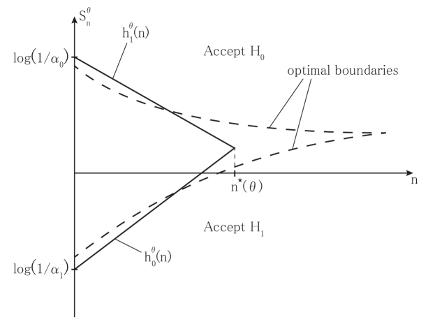
The importance of this result cannot be overstated since the very simple test proposed by Lorden is almost optimal. At the same time, the optimal test can also be computed using Bellman’s backward induction algorithm since the optimal sequential test is truncated, i.e., has bounded maximal sample size, as shown by Kiefer and Weiss (1957). For one-parameter exponential families, the optimal bounds are curved in the $(S_{n},n)$ plane, where $S_{n}=\sum_{t=1}^{n}X_{i}$, and finding them typically requires substantial computation. In contrast, Lorden’s 2-SPRT approximates optimal curved boundaries with simple linear ones, so the continuation region is a triangle, as shown in Figure 1, below.

Lorden (1976) performed an extensive performance analysis for testing the mean $\theta$ of the Gaussian distribution $X_{n}\sim{\mathcal{N}}(\theta,1)$ with the hypotheses $\operatorname{\mathcal{H}}_{i}:\theta=\theta_{i}$, ($i=0,1$) in the symmetric case where $\alpha_{0}=\alpha_{1}$ and ${\mathsf{G}}\sim{\mathcal{N}}(\theta_{\star},1)$, $\theta_{\star}=(\theta_{0}+\theta_{1})/2$. The conclusion is that the $2$-SPRT performs very closely to the optimal test with its curved boundaries obtained using backward induction. The efficiency depends on the error probabilities, but it was over $99\%$ in all his performed experiments. Similar results were obtained by Huffman (1983) for the exponential example $f_{\theta}(x)=\theta e^{-\theta x}$, $x\geqslant 0$, $\theta>0$. Here the $2$-SPRT has efficiency over $98\%$ and almost always over $99\%$ for a broad range of error probabilities and parameter values.

The results of Theorem 4 can be extended to the multiple hypothesis case. Specifically, the modified matrix SPRT defined in (32)–(34) is also third-order asymptotically optimal as ${\alpha_{\rm max}}=\max_{1\leqslant i\leqslant N}\alpha_{i}\to 0$ in the class of tests

$${\mathbb{C}}({\bm{\alpha}})=\left\{\delta:\alpha_{i}(\delta)\leqslant\alpha_{i}~{}\text{for}~{}i=0,1,\dots,N\right\},$$

where $\alpha_{i}(\delta)={\mathsf{P}}_{i}(d\neq i)$ and ${\bm{\alpha}}=(\alpha_{0},\alpha_{1},\dots,\alpha_{N})$ is a vector of given error probabilities, c.f. Tartakovsky, Nikiforov, and Basseville (2015, Theorem 5.3.3 (page 240)).

Lorden’s results have led to further research related to the minimax Kiefer–Weiss problem of establishing near-optimal solutions for the least favorable intermediate distribution ${\mathsf{G}}$ in the single-parameter exponential family.

We now consider the parametric case ${\mathsf{G}}={\mathsf{P}}_{\theta}$, ${\mathsf{P}}_{i}={\mathsf{P}}_{\theta_{i}}$ where the hypotheses are $H_{0}:\theta=\theta_{0}$ and $H_{1}:\theta=\theta_{1}$, $\theta_{0}<\theta_{1}$. Let $\theta$ be an arbitrary point belonging to the interval $(\theta_{0},\theta_{1})$ and let $\delta^{\star}(\theta)=(d^{\star}(\theta),T^{\star}(\theta))$ denote the $2$-SPRT tuned to $\theta$. In other words, $T^{\star}(\theta)=\min(T_{0}^{\theta},T_{1}^{\theta})$, where the $T_{i}^{\theta}$’s are defined by (35) with the LLRs $\lambda_{i}^{\theta}(n)=\log[{\mathrm{d}}{\mathsf{P}}_{\theta}^{n}/{\mathrm{d}}{\mathsf{P}}_{\theta_{i}}^{n}]({\mathbf{X}}^{n})$, $i=0,1$, tuned to $\theta$.

Theorem 4 implies that the $2$-SPRT $\delta^{\star}(\theta)$ is third-order asymptotically optimal in terms of minimizing ${\mathsf{E}}_{\theta}[T]$ at the intermediate point $\theta\in(\theta_{0},\theta_{1})$ when the second moments ${\mathsf{E}}_{\theta}|\lambda_{0}^{\theta}(1)|^{2}$ and ${\mathsf{E}}_{\theta}|\lambda_{1}^{\theta}(1)|^{2}$ are finite and the thresholds $a_{i}$ are selected in such a way that the error probabilities are either exactly equal to the given numbers $\alpha_{i}$ or at least close to $\alpha_{i}$, the latter requirement being a difficult task. However, setting $a_{i}=|\log\alpha_{i}|$ embeds the $2$-SPRT into the class ${\mathbb{C}}(\alpha_{0},\alpha_{1})$ and Theorem 4 suggests that if one can find a nearly least favorable point $\theta^{*}$, i.e. $\theta^{*}$ can be selected so that $\sup_{\theta}{\mathsf{E}}_{\theta}[T^{\star}(\theta^{*})]\approx{\mathsf{E}}_{\theta^{*}}[T^{\star}(\theta^{*})]$, then $\delta^{\star}(\theta^{*})$ is an approximate solution to the Kiefer–Weiss problem of minimizing $\sup_{\theta}{\mathsf{E}}_{\theta}[T]$.

Consider the single-parameter exponential family $\{f_{\theta}(x),\theta\in\Theta\}$ assuming that the common density $f_{\theta}(x)$ of the i.i.d. observations $X_{1},X_{2},\dots$ is such that

$$\frac{f_{\theta}(X_{n})}{f_{\widetilde{\theta}}(X_{n})}=\exp\left\{(\theta-\widetilde{\theta})X_{n}-(b(\theta)-b(\widetilde{\theta}))\right\},\quad n=1,2,\dots$$ (37)

where $b(\theta)$ is a convex and infinitely differentiable function on $\widetilde{\Theta}\subset\Theta$. A simple calculation shows that ${\mathsf{E}}_{\theta}[X_{1}]=\overset{\bm{.}}{b}(\theta)$ , $\sigma^{2}_{\theta}={\mathsf{var}}_{\theta}(X_{1})=\ddot{b}(\theta)$, and the Kullback–Leibler numbers are

$$I(\theta,\theta_{i})=(\theta-\theta_{i})\overset{\bm{.}}{b}(\theta)-(b(\theta)-b(\theta_{i})).$$

Without loss of generality we assume that $\inf_{\theta\in\widetilde{\Theta}}\sigma^{2}_{\theta}>0$, $\sup_{\theta\in\widetilde{\Theta}}\sigma^{2}_{\theta}<\infty$.

It turns out that it is possible to determine the nearly least favorable point $\theta_{\star}(\alpha_{0},\alpha_{1},\theta_{0},\theta_{1})$ such that the $2$-SPRT with thresholds $a_{i}=\log(1/\alpha_{i})$ is second-order asymptotically minimax for the exponential family (37), i.e., the residual term in the difference between the expectation of the sample size of the optimal test and the 2-SPRT is of order $O(1)$ for small error probabilities. This problem was first addressed by Huffman (1983) who suggested the $\theta_{\star}(\alpha_{0},\alpha_{1},\theta_{0},\theta_{1})$ which leads to the residual term of order $o(|\log{\alpha_{\rm max}}|^{1/2})$. This result was strengthened by Dragalin and Novikov (1987) who have established the second-order optimality of Huffman’s version of 2-SPRT. Specifically, writing

$$S_{n}^{\theta}=S_{n}-{\mathsf{E}}_{\theta}[X_{1}]n\equiv S_{n}-\overset{\bm{.}}{b}(\theta)n$$

and noting that

$$\lambda_{i}^{\theta}(n):=\sum_{t=1}^{n}\log\left[\frac{f_{\theta}(X_{t})}{f_{\theta_{i}}(X_{t})}\right]=(\theta-\theta_{i})S_{n}^{\theta}+I(\theta,\theta_{i})n,$$

it is easy to see that the stopping times $T_{i}^{\theta}$ can be written as

$\displaystyle T_{0}^{\theta}$ $\displaystyle=\inf\left\{n:\lambda_{1}^{\theta}(n)\geqslant|\log\alpha_{1}|\right\}=\inf\left\{n:S_{n}^{\theta}\leqslant(\theta_{1}-\theta)^{-1}[-|\log\alpha_{1}|+I(\theta,\theta_{1})n]\right\},$
$\displaystyle T_{1}^{\theta}$ $\displaystyle=\inf\left\{n:\lambda_{0}^{\theta}(n)\geqslant|\log\alpha_{0}|\right\}=\inf\left\{n:S_{n}^{\theta}\geqslant(\theta-\theta_{0})^{-1}[|\log\alpha_{0}|-I(\theta,\theta_{0})n]\right\}.$

Therefore, the stopping time $T^{\star}(\theta)=\min(T_{0}^{\theta},T_{1}^{\theta})$ of the $2$-SPRT tuned to $\theta$ can be represented as

$$T^{\star}(\theta)=\min\left\{n\geqslant 1:S_{n}^{\theta}\notin(h_{0}^{\theta}(n),h_{1}^{\theta}(n))\right\},$$

where the boundaries $h_{1}^{\theta}(n)$ and $h_{0}^{\theta}(n)$ are linear functions of $n$:

$$h_{1}^{\theta}(n)=\frac{|\log\alpha_{0}|-I(\theta,\theta_{0})\,n}{\theta-\theta_{0}},\quad h_{0}^{\theta}(n)=\frac{-|\log\alpha_{1}|+I(\theta,\theta_{1})\,n}{\theta_{1}-\theta}.$$

Define $\gamma(\theta,\theta_{i})=(\theta-\theta_{i})/I(\theta,\theta_{i})$. Since $\gamma(\theta,\theta_{1})<0<\gamma(\theta,\theta_{0})$, it is easily verified that these boundaries intersect at the point

$$n^{\star}(\theta)=\frac{1}{\gamma(\theta,\theta_{0})+|\gamma(\theta,\theta_{1})|}\left[\frac{\gamma(\theta,\theta_{0})}{I(\theta,\theta_{1})}|\log\alpha_{1}|+\frac{|\gamma(\theta,\theta_{1})|}{I(\theta,\theta_{0})}|\log\alpha_{0}|\right].$$ (38)

Therefore, the region of continuation of observations is a triangle, as shown in Figure 1. This means that the $2$-SPRT is a truncated test with the maximal number of steps $n^{\star}(\theta)$. Figure 1 also shows the typical curved boundaries of the optimal truncated test that can be computed using Bellman’s backward induction.

Refer to caption
Figure 1: The boundaries $h_{1}^{\theta}(n)$ and $h_{0}^{\theta}(n)$ of the $2$-SPRT (solid) and optimal boundaries (dashed) as functions of $n$.

By Corollary 5.3.1 in Tartakovsky, Nikiforov, and Basseville (2015), the $2$-SPRT $\delta^{\star}(\theta)$ minimizes all positive moments of the stopping time distribution at the point $\theta$ to first order (as $\alpha_{\max}\to 0$) in the class ${\mathbb{C}}(\alpha_{0},\alpha_{1})$ as long as the ratio $|\log\alpha_{0}|/|\log\alpha_{1}|$ is bounded away from zero and infinity,

$$\lim_{\alpha_{\max}\to 0}\frac{|\log\alpha_{0}|}{|\log\alpha_{1}|}=c,\quad 0<c<\infty,$$ (39)

and the following asymptotics hold:

$$\inf_{\delta\in{\mathbb{C}}(\alpha_{0},\alpha_{1})}{\mathsf{E}}_{\theta}[T]\sim{\mathsf{E}}_{\theta}[T^{\star}(\theta)]\sim\min\left[\frac{|\log\alpha_{1}|}{I(\theta,\theta_{0})},\frac{|\log\alpha_{0}|}{I(\theta,\theta_{1})}\right]\quad\text{as}~{}~{}\alpha_{\max}\to 0.$$ (40)

The right-hand side of the asymptotic equality (40) is maximized at $\theta=\theta^{*}$ that satisfies the equation

$$\frac{|\log\alpha_{1}|}{I(\theta^{*},\theta_{0})}=\frac{|\log\alpha_{0}|}{I(\theta^{*},\theta_{1})}(\equiv n^{\star}(\theta^{*}))$$ (41)

in which case

$$\inf_{\delta\in{\mathbb{C}}(\alpha_{0},\alpha_{1})}{\mathsf{E}}_{\theta^{*}}[T]\sim{\mathsf{E}}_{\theta^{*}}[T^{\star}(\theta^{*})]\sim n^{\star}(\theta^{*})\quad\text{as}~{}~{}\alpha_{\max}\to 0$$

and $\sup_{\theta}{\mathsf{E}}_{\theta}[T^{\star}(\theta^{*})]\approx n^{\star}(\theta^{*})$. Next, we observe that the function $n^{\star}(\theta)$ attains its minimum at the point $\theta=\theta^{*}$. Thus, the point $\theta^{*}$ has two properties simultaneously – it minimizes the time of truncation $\min_{\theta\in(\theta_{0},\theta_{1})}n^{\star}(\theta)=n^{\star}(\theta^{*})$ on one hand, and approximately maximizes the expected sample size of the $2$-SPRT on the other hand. Hence, we may expect that $\delta^{\star}(\theta^{*})$ is asymptotically minimax. This is indeed the case

$$\inf_{\delta\in{\mathbb{C}}(\alpha_{0},\alpha_{1})}~{}\sup_{\theta\in\Theta}{\mathsf{E}}_{\theta}[T]\sim\sup_{\theta\in\Theta}{\mathsf{E}}_{\theta}[T^{\star}(\theta^{*})]\sim{\mathsf{E}}_{\theta^{*}}[T^{\star}(\theta^{*})]\sim n^{\star}(\theta^{*}),$$

so that the $2$-SPRT tuned to the point $\theta^{*}$, which is found from (41), is first-order minimax. However, with this choice the supremum of ${\mathsf{E}}_{\theta}[T^{\star}(\theta^{*})]$ over $\theta$ is attained at the point $\theta^{*}$ only to within the term $o(n^{\star}(\theta^{*}))$. This result can be improved to within $O(1)$ by choosing the tuning point in a slightly different manner as $\theta_{\star}=\theta^{*}+C\cdot n^{\star}(\theta^{*})^{-1/2}$. Specifically, Huffman (1983) suggested to use the tuning point

$$\theta_{\star}=\theta^{*}+\frac{r^{*}}{\sigma_{\theta^{*}}\sqrt{n^{\star}(\theta^{*})}},$$ (42)

where $r^{*}$ is a solution of the equation

$$\Phi(r^{*})=\frac{|\gamma(\theta^{*},\theta_{1})|}{|\gamma(\theta^{*},\theta_{1})|+\gamma(\theta^{*},\theta_{0})}$$

($\Phi(x)$ is the cdf of the standard normal variable). The residual term in Huffman’s approximation is of order $o(n^{\star}(\theta^{\star})^{1/2})$. Dragalin and Novikov (1987) found a more accurate estimate of the residual term in the expansion for the expected sample size showing that it is of order $O(1)$.

The following theorem states the final result. We recall that $n^{\star}(\theta)$ is defined in (38) and, as usual, we write $\varphi(x)={\mathrm{d}}\Phi(x)/{\mathrm{d}}x$ for density of the standard normal distribution $\Phi(x)$.

Theorem 5.

Let the observed random variables $X_{1},X_{2},\dots$ be i.i.d. from the exponential family (37). Let the thresholds in the $2$-SPRT be selected as $a_{1}=|\log\alpha_{1}|$ and $a_{0}=|\log\alpha_{0}|$, and let the tuning point $\theta_{\star}$ be as in (42). If the condition (39) holds, then as $\alpha_{\max}\to 0$,

$\displaystyle{\mathsf{E}}_{\theta_{\star}}[T^{\star}(\theta_{\star})]$ $\displaystyle=n^{\star}(\theta^{*})-\sigma_{\theta^{*}}\left[(\gamma(\theta^{*},\theta_{0})+|\gamma(\theta^{*},\theta_{1})|)\varphi(r^{*})\sqrt{n^{\star}(\theta^{*})}\right]+O(1),$
$\displaystyle\sup_{\theta\in\Theta}{\mathsf{E}}_{\theta}[T^{\star}(\theta_{\star})]$ $\displaystyle={\mathsf{E}}_{\theta_{\star}}[T^{\star}(\theta_{\star})]+O(1),$
$\displaystyle\inf_{\delta\in{\mathbb{C}}(\alpha_{0},\alpha_{1})}\sup_{\theta\in\Theta}{\mathsf{E}}_{\theta}[T]$ $\displaystyle={\mathsf{E}}_{\theta_{\star}}[T^{\star}(\theta_{\star})]+O(1).$

Therefore, the $2$-SPRT $\delta^{\star}(\theta_{\star})$ is second-order asymptotically minimax.

As we have already pointed out, the formulas $a_{i}=|\log\alpha_{i}|$, which guarantee the inequalities $\alpha_{i}(\delta^{\star}(\theta))\leqslant\alpha_{i}$, are rather conservative. An improvement can be obtained by observing that

$\displaystyle\alpha_{1}(\delta^{\star}(\theta))$ $\displaystyle={\mathsf{P}}_{\theta}(T^{\star}=T_{0}^{\theta})e^{-a_{1}}{\mathsf{E}}_{\theta}\left\{e^{-(a_{1}-\lambda_{1}^{\theta}(T_{0}^{\theta}))}|T^{\star}=T_{0}^{\theta}\right\},$
$\displaystyle\alpha_{0}(\delta^{\star}(\theta))$ $\displaystyle={\mathsf{P}}_{\theta}(T^{\star}=T_{1}^{\theta})e^{-a_{0}}{\mathsf{E}}_{\theta}\left\{e^{-(a_{0}-\lambda_{0}^{\theta}(T_{1}^{\theta}))}|T^{\star}=T_{1}^{\theta}\right\}$

and by noticing that asymptotically as $a_{i}\to\infty$,

$\displaystyle{\mathsf{P}}_{\theta}(T^{\star}=T_{1}^{\theta})\to\frac{|\gamma(\theta,\theta_{1})|}{|\gamma(\theta,\theta_{1})|+\gamma(\theta,\theta_{0})},\quad{\mathsf{P}}_{\theta}(T^{\star}=T_{0}^{\theta})\to\frac{\gamma(\theta,\theta_{0})}{|\gamma(\theta,\theta_{1})|+\gamma(\theta,\theta_{0})},$
$\displaystyle{\mathsf{E}}_{\theta}\left\{e^{-(a_{0}-\lambda_{0}^{\theta}(T_{1}^{\theta}))}|T^{\star}=T_{1}^{\theta}\right\}\to\zeta_{0}^{\theta},\quad{\mathsf{E}}_{\theta}\left\{e^{-(a_{1}-\lambda_{1}^{\theta}(T_{0}^{\theta}))}|T^{\star}=T_{0}^{\theta}\right\}\to\zeta_{1}^{\theta}.$

For the nonarithmetic case $\zeta_{i}^{\theta}$ can be computed using the renewal-theoretic argument similar to (17) and (19):

$$\zeta_{i}^{\theta}=\frac{1}{I(\theta,\theta_{i})}\exp\left\{-\sum_{n=1}^{\infty}\frac{1}{n}\left[{\mathsf{P}}_{\theta}(\lambda_{i}^{\theta}(n)>0)+{\mathsf{P}}_{i}(\lambda_{i}^{\theta}(n)\leqslant 0)\right]\right\}.$$

This yields

$$\alpha_{0}(\delta^{\star}(\theta))\sim\frac{|\gamma(\theta,\theta_{1})|}{|\gamma(\theta,\theta_{1})|+\gamma(\theta,\theta_{0})}\zeta_{0}^{\theta}e^{-a_{0}},\quad\alpha_{1}(\delta^{\star}(\theta))\sim\frac{\gamma(\theta,\theta_{0})}{|\gamma(\theta,\theta_{1})|+\gamma(\theta,\theta_{0})}\zeta_{1}^{\theta}e^{-a_{1}}.$$

2.6 Near Uniform Optimality of the GLR SPRT for Composite Hypotheses

For practical purposes, it is much more important to design tests that would minimize the expected sample size ${\mathsf{E}}_{\theta}[T]$ for all possible parameter values (i.e., uniformly optimal) rather than to solve the minimax Kiefer–Weiss problem of minimizing ${\mathsf{E}}_{\theta}[T]$ at a least favorable point. In this section, our ultimate goal is to discuss how to design sequential tests that are at least approximately uniformly optimal for small error probabilities or asymptotically Bayesian for small cost of observations for testing composite hypotheses. Assume that the sequence of i.i.d. observations $X_{1},X_{2},\dots$ comes from a common distribution ${\mathsf{P}}_{\theta}$ with density $f_{\theta}(x)$ with respect to some non-degenerate sigma-finite measure, where the $\ell$-dimensional parameter $\theta=(\theta_{1},\dots,\theta_{\ell})$ belongs to a subset $\Theta$ of the Euclidean space $\mathbb{R}^{\ell}$. The parameter space $\Theta$ is split into $3$ disjoint sets $\Theta_{0},\Theta_{1}$ and ${\mathsf{I}_{\mathrm{in}}}$, i.e., $\Theta=\Theta_{0}\,{\textstyle\bigcup}\,\Theta_{2}\,{\textstyle\bigcup}\,{\mathsf{I}_{\mathrm{in}}}$. The problem is to test the two composite hypotheses $\operatorname{\mathcal{H}}_{0}:\theta\in\Theta_{0}$ against $\operatorname{\mathcal{H}}_{1}:\theta\in\Theta_{1}$. The subset ${\mathsf{I}_{\mathrm{in}}}$ of $\Theta$ represents an indifference zone where the loss $L(\theta,d)$ associated with correct or incorrect decisions $d$ is zero, i.e., no constraints on the probabilities ${\mathsf{P}}_{\theta}(d=i)$ are imposed if $\theta\in{\mathsf{I}_{\mathrm{in}}}$. The indifference zone is usually introduced since, in most applications, the correct action is not critical and often not even possible when the hypotheses are very close. However, in principle ${\mathsf{I}_{\mathrm{in}}}$ may be an empty set.

We are interested in finding a sequential test $\delta=(T,d)$ that minimizes the expected sample size ${\mathsf{E}}_{\theta}[T]$ uniformly for all $\theta\in\Theta$ in the class of tests ${\mathbb{C}}(\alpha_{0},\alpha_{1})$ in which the maximal error probabilities $\sup_{\theta\in\Theta_{i}}{\mathsf{P}}_{\theta}(d\neq i)$ are upper-bounded by the given values:

$${\mathbb{C}}(\alpha_{0},\alpha_{1})=\left\{\delta:\sup_{\theta\in\Theta_{0}}{\mathsf{P}}_{\theta}(d=1)\leqslant\alpha_{0}~{}~{}\text{and}~{}~{}\sup_{\theta\in\Theta_{1}}{\mathsf{P}}_{\theta}(d=0)\leqslant\alpha_{1}\right\}.$$ (43)

In other words, we are interested in the following frequentist problem: Find a test $\delta_{\rm opt}$ such that

$$\inf_{\delta\in{\mathbb{C}}(\alpha_{0},\alpha_{1})}{\mathsf{E}}_{\theta}[T]={\mathsf{E}}_{\theta}[T_{\rm opt}]\quad\text{uniformly in}~{}~{}\theta\in\Theta.$$ (44)

Unfortunately, such a uniformly optimal solution does not exist, and one has to resort to finding asymptotic approximations for small error probabilities. In the frequentist setting, it is possible to find first-order asymptotically optimal tests that satisfy

$$\lim_{{\alpha_{\rm max}}\to 0}\frac{\inf_{\delta\in{\mathbb{C}}(\alpha_{0},\alpha_{1})}{\mathsf{E}}_{\theta}[T]}{{\mathsf{E}}_{\theta}[T]}=1\quad\text{for all}~{}~{}\theta\in\Theta.$$ (45)

In addition to the frequentist problems (44)-(45), it is of interest to consider a Bayesian approach putting an a priori distribution $W(\theta)$ on $\Theta$ with a cost $c$ per observation and a loss function $L(\theta)$ at the point $\theta$ associated with accepting the incorrect hypothesis and find asymptotically optimal tests when the cost $c$ is small. The Bayes average (integrated) risk of a sequential test $\delta=(T,d)$ is

$$\rho_{c}^{W}(\delta)=\int_{\theta\leqslant\theta_{0}}L(\theta){\mathsf{P}}_{\theta}(d=1)\,W({\mathrm{d}}\theta)+\int_{\theta\geqslant\theta_{1}}L(\theta){\mathsf{P}}_{\theta}(d=0)\,W({\mathrm{d}}\theta)+c\int_{\Theta}{\mathsf{E}}_{\theta}[T]\,W({\mathrm{d}}\theta).$$

It turns out that in the Bayesian context, it is possible to find tests that are not only asymptotically (as $c\to 0$) first-order optimal, $\inf_{\delta}\rho_{c}^{W}(\delta)=\rho_{c}^{W}(\delta)(1+o(1))$, but also second-order optimal, i.e., $\inf_{\delta}\rho_{c}^{W}(\delta)=\rho_{c}^{W}(\delta)+O(c)$ and even third-order optimal, i.e., $\inf_{\delta}\rho_{c}^{W}(\delta)=\rho_{c}^{W}(\delta)+o(c)$.

In the case of the one-parameter exponential family (37), using optimal stopping theory, it can be shown that the optimal Bayesian test $\delta_{\rm opt}=(T_{\rm opt},d_{\rm opt})$ is

$$T_{\rm opt}=\inf\left\{n\geqslant 1:(S_{n},n)\in\mathcal{B}_{c}\right\},\quad d_{\rm opt}=j~{}~{}\text{if}~{}(S_{n},n)\in\mathcal{B}_{c}^{j},\quad j=0,1,$$

where $S_{n}=X_{1}+\cdots+X_{n}$ and $\mathcal{B}_{c}=\mathcal{B}_{c}^{0}\,{\textstyle\bigcup}\,\mathcal{B}_{c}^{1}$ is a set that can be found numerically.

Schwarz (1962) derived the test $\delta^{\star}(\hat{\theta})$ with $\hat{\theta}=\{\hat{\theta}_{n}\}$ being the maximum likelihood estimator (MLE) of $\theta$, as an asymptotic solution as $c\to 0$ to the Bayesian problem with the $0-1$ loss function. Specifically, the a posteriori risk of stopping is

$$R_{n}^{\rm st}(S_{n})=\min_{i=0,1}\left\{\frac{\int_{\Theta_{i}}\exp\left\{\theta S_{n}-nb(\theta)\right\}\,W({\mathrm{d}}\theta)}{\int_{\Theta}\exp\left\{\theta S_{n}-nb(\theta)\right\}\,W({\mathrm{d}}\theta)}\right\},$$ (46)

where $\Theta_{0}=\{\theta\leqslant\theta_{0}\}$, $\Theta_{1}=\{\theta\geqslant\theta_{1}\}$. Schwarz showed that $\mathcal{B}_{c}/|\log c|\to\mathcal{B}_{0}$ as $c\to 0$ and proposed a simple procedure: continue sampling until $R_{n}^{\rm st}(S_{n})$ is less than $c$ and upon stopping accept the hypothesis for which the minimum is attained in (46). Denote this procedure by $\widetilde{\delta}(c)=(\widetilde{T}(c),\widetilde{d}(c))$. Applying Laplace’s asymptotic integration method to evaluate the integrals in (46) leads to the likelihood ratio test where the true parameter is replaced by the MLE $\hat{\theta}_{n}$. This approximation prescribes stopping sampling at the time $\widehat{T}(\hat{\theta})=\min(\widehat{T}_{0}(\hat{\theta}),\widehat{T}_{1}(\hat{\theta}))$, where

$\displaystyle\widehat{T}_{i}(\hat{\theta})=\inf\left\{n:\sup_{\theta\in\Theta}[\theta S_{n}-nb(\theta)]-[\theta_{i}S_{n}-nb(\theta_{i})]\geqslant|\log c|\right\}.$ (47)

The terminal decision rule $\hat{d}(\hat{\theta})$ of the test $\hat{\delta}(\hat{\theta})=(\widehat{T}(\hat{\theta}),\hat{d}(\hat{\theta}))$ accepts $\operatorname{\mathcal{H}}_{0}$ if $\hat{\theta}_{\widehat{T}}<\theta^{*}$, where $\theta^{*}$ is such that $I(\theta^{*},\theta_{0})=I(\theta^{*},\theta_{1})$. Note also that

$$\widehat{T}=\inf\left\{n\geqslant 1:n\max[I(\hat{\theta}_{n},\theta_{0}),I(\hat{\theta}_{n},\theta_{1})]\geqslant|\log c|\right\}.$$ (48)

The tests which use the maximum likelihood estimators of unknown parameters are usually referred to as the Generalized Sequential Likelihood Ratio Tests (GSLRT).

Wong (1968) showed that the GSLRT $\hat{\delta}$ is first-order asymptotically Bayes as $c\to 0$:

$$\rho_{c}^{W}(\hat{\delta})\sim\inf_{\delta}\rho_{c}^{W}(\delta)\sim c|\log c|\int_{\Theta}\frac{W({\mathrm{d}}\theta)}{I_{\max}(\theta)},\quad{\mathsf{E}}_{\theta}[\widehat{T}]\sim\frac{|\log c|}{I_{\max}(\theta)}\quad\text{for every}~{}~{}\theta\in\Theta,$$

where $I_{\max}(\theta)=\max\left\{I(\theta,\theta_{0}),I(\theta,\theta_{1})\right\}$.

Kiefer and Sacks (1963) showed that the procedure $\widetilde{\delta}(c)=(\widetilde{T}(c),\widetilde{d}(c))$ with the stopping time

$$\widetilde{T}(c)=\inf\left\{n\geqslant 1:R_{n}^{\rm st}(S_{n})\leqslant c\right\}$$

proposed by Schwarz (1962), is also first-order asymptotically Bayes, i.e., for any prior distribution $W$, $\rho_{c}^{W}(\widetilde{\delta}(c))\sim\inf_{\delta}\rho_{c}^{W}(\delta)$ as $c\to 0$. Lorden (1967) refined this result by introducing the stopping region as the first $n$ such that $R_{n}^{\rm st}(S_{n})\leqslant Qc$, where $Q$ is a positive constant, and showed that it can be made second-order asymptotically optimal, i.e., $\inf_{\delta}\rho_{c}^{W}(\delta)=\rho_{c}^{W}(\widetilde{\delta}(Qc))+O(c)$ as $c\to 0$, while $\inf_{\delta}\rho_{c}^{W}(\delta)=O(c|\log c|)$. Notice that the problem addressed by Lorden (1967) is much more general than what we are discussing here, since it encompasses general i.i.d. models – not only exponential families – and multiple-decision cases.

A breakthrough in the Bayesian theory for testing separated hypotheses about the parameter of the one-parameter exponential family (37) was achieved by Lorden (1977b) (an unpublished manuscript), where he showed that the family of GSLRTs can be designed to guarantee the third-order asymptotic optimality, i.e., to attain the Bayes risk to within $o(c)$ as $c\to 0$. Lorden gave sufficient conditions for families of tests to be third-order asymptotically Bayes and examples of such procedures based not only on the GLR approach but also on mixtures of likelihood ratios. In addition, the error probabilities of the GSLRTs have been evaluated asymptotically as a consequence of a general theorem on boundary-crossing probabilities. Due to the importance of this work, we give a more detailed overview of Lorden’s theory. Notice that the paper Lorden (1977b) is an extension to a continuous parameter case of the results obtained by Lorden (1977a) for multiple discrete cases that we discussed in Subsection 2.4.

The hypotheses to be tested are $\operatorname{\mathcal{H}}_{0}:\underline{\theta}\leqslant\theta\leqslant\theta_{0}$ and $\operatorname{\mathcal{H}}_{1}:\overline{\theta}\geqslant\theta\geqslant\theta_{1}$, where $\underline{\theta}$ and $\overline{\theta}$ are interior points of the natural parameter space $\Theta$. Let $\hat{\theta}_{n}\in[\underline{\theta},\overline{\theta}]$ be the MLE that maximizes the likelihood over $\theta$ in $[\underline{\theta},\overline{\theta}]$. Lorden’s GSLRT stops at $\widehat{T}$ which is the minimum of the Markov times $\widehat{T}_{0},\widehat{T}_{1}$ defined as

$\displaystyle\widehat{T}_{0}(\hat{\theta})$ $\displaystyle=\inf\left\{n\geqslant 1:\sum_{k=1}^{n}\log\left[\frac{f_{\hat{\theta}_{n}}(X_{k})}{f_{\theta_{0}}(X_{k})}~{}h_{0}(\hat{\theta}_{n})\right]\geqslant a~{}\text{and}~{}\hat{\theta}_{n}\geqslant\theta^{*}\right\},$ (49)
$\displaystyle\widehat{T}_{1}(\hat{\theta})$ $\displaystyle=\inf\left\{n\geqslant 1:\sum_{k=1}^{n}\log\left[\frac{f_{\hat{\theta}_{n}}(X_{k})}{f_{\theta_{1}}(X_{k})}~{}h_{1}(\hat{\theta}_{n})\right]\geqslant a~{}\text{and}~{}\hat{\theta}_{n}\leqslant\theta^{*}\right\},$

where $a$ is a threshold, $\theta^{*}$ satisfies $I(\theta^{*},\theta_{0})=I(\theta^{*},\theta_{1})$, and $h_{0},h_{1}$ are positive continuous functions on $[\theta^{*},\overline{\theta}],[\underline{\theta},\theta^{*}]$, respectively. The hypothesis $\operatorname{\mathcal{H}}_{i}$ is rejected when $\widehat{T}=\widehat{T}_{i}$. To summarize, Lorden’s family of GSPRTs is defined as

$$\widehat{T}(\hat{\theta})=\min\left\{\widehat{T}_{0}(\hat{\theta}),\widehat{T}_{1}(\hat{\theta})\right\},\quad\hat{d}=\begin{cases}0&\text{if}~{}~{}\widehat{T}(\hat{\theta})=\widehat{T}_{1}(\hat{\theta})\\ 1&\text{if}~{}\widehat{T}(\hat{\theta})=\widehat{T}_{0}(\hat{\theta})\end{cases},$$ (50)

with the $\widehat{T}_{i}(\hat{\theta})$’s in (49).

Write

$$\lambda_{n}(\theta,\theta_{i})=\sum_{k=1}^{n}\log\left[\frac{f_{\theta}(X_{k})}{f_{\theta_{i}}(X_{k})}\right]=(\theta-\theta_{i})S_{n}-[b(\theta)-b(\theta_{i})]n$$

for the LLR between points $\theta$ and $\theta_{i}$.

Lorden assumes that the prior distribution $W(\theta)$ has a continuous density $w(\theta)$ positive on $[\underline{\theta},\overline{\theta}]$, and that the loss $L(\theta)$ equals zero in the indifference zone $(\theta_{0},\theta_{1})$ and is continuous and positive elsewhere and bounded away from 00 on $[\underline{\theta},\theta_{0}]\,{\textstyle\bigcup}\,[\theta_{1},\overline{\theta}]$. The main results in (Lorden 1977b, Theorem 1) can be briefly outlined as follows.

(i)

Under these assumptions the family of GSLRTs defined by (49)–(50) with $a=|\log c|-\tfrac{1}{2}\log|\log c|$ is second-order asymptotically optimal, i.e.,

$$\rho_{c}^{w}(\hat{\delta})=\inf_{\delta}\rho_{c}^{w}(\delta)+O(c)\quad\text{as}~{}c\to 0,$$

where $\rho_{c}^{w}(\delta)$ is the average risk of the test $\delta=(T,d)$:

$$\rho_{c}^{w}(\delta)=\int_{\underline{\theta}}^{\theta_{0}}L(\theta){\mathsf{P}}_{\theta}(d=1)w(\theta)\,{\mathrm{d}}\theta+\int_{\theta_{1}}^{\overline{\theta}}L(\theta){\mathsf{P}}_{\theta}(d=0)w(\theta)\,{\mathrm{d}}\theta+c\int_{\underline{\theta}}^{\overline{\theta}}{\mathsf{E}}_{\theta}[T]w(\theta)\,{\mathrm{d}}\theta.$$
(ii)

This result can be improved from $O(c)$ to $o(c)$, i.e., to the third order

$$\rho_{c}^{w}(\hat{\delta})=\inf_{\delta}\rho_{c}^{w}(\delta)+o(c)\quad\text{as}~{}c\to 0,$$

making the right choice of the functions $h_{0}$ and $h_{1}$ by setting

$$h_{i}(\theta)=\sqrt{\frac{2\pi}{I^{3}(\theta,\theta_{i})\ddot{b}(\theta)}}~{}\frac{w(\theta)|\overset{\bm{.}}{b}(\theta)-\overset{\bm{.}}{b}(\theta_{i})|}{w(\theta_{i})L(\theta_{i})\zeta(\theta,\theta_{i})},\quad i=0,1,$$

where $\zeta(\theta,\theta_{i})={\mathcal{L}}(\theta,\theta_{i})/I(\theta,\theta_{i})$ is a correction for the overshoot over the boundary, the factor which is the subject of renewal theory. Specifically,

$$\zeta(\theta,\theta_{i})=\lim_{a\to\infty}{\mathsf{E}}_{\theta}\exp\left\{-[\lambda_{\tau_{a}}(\theta,\theta_{i})-a]\right\},\quad\tau_{a}=\inf\left\{n:\lambda_{n}(\theta,\theta_{i})\geqslant a\right\},$$ (51)

where in the non-arithmetic case $\zeta(\theta,\theta_{i})$ can be computed as

$$\zeta(\theta,\theta_{i})=\frac{1}{I(\theta,\theta_{i})}\exp\left\{-\sum_{n=1}^{\infty}\frac{1}{n}\left[{\mathsf{P}}_{\theta}(\lambda_{n}(\theta,\theta_{i})\leqslant 0)+{\mathsf{P}}_{\theta_{i}}(\lambda_{n}(\theta,\theta_{i})>0)\right]\right\}.$$ (52)

Since the Bayes average risk $\inf_{\delta}\rho_{c}^{w}(\delta)$ is of order $c|\log c|$, this implies that the asymptotic relative efficiency $\mathcal{E}_{c}=[\rho_{c}^{w}(\hat{\delta})-\inf_{\delta}\rho_{c}^{w}(\delta)]/\rho_{c}^{w}(\hat{\delta})$ of Lorden’s test is of order $1-o(1/|\log c|)$ as $c\to 0$.

Note the crucial difference between Schwarz’s GSLRT (47) and Lorden’s GSLRT (50). While in the Schwarz test $h_{i}\equiv 1$ and the threshold is $a=|\log c|$, in the Lorden test, there are two innovations. First, the threshold is smaller by $\tfrac{1}{2}\log|\log c|$, and second, there are adaptive weights $h_{i}(\hat{\theta}_{n})$ in the GLR statistic. Since the stopping times $\widehat{T}_{i}$ can be obviously written as

$\displaystyle\widehat{T}_{0}(\hat{\theta})$ $\displaystyle=\inf\left\{n\geqslant 1:\lambda_{n}(\hat{\theta}_{n},\theta_{0})\geqslant a-\log h_{0}(\hat{\theta}_{n})~{}\text{and}~{}\hat{\theta}_{n}\geqslant\theta^{*}\right\},$ (53)
$\displaystyle\widehat{T}_{1}(\hat{\theta})$ $\displaystyle=\inf\left\{n\geqslant 1:\lambda_{n}(\hat{\theta}_{n},\theta_{1})\geqslant a-\log h_{1}(\hat{\theta}_{n})~{}\text{and}~{}\hat{\theta}_{n}\leqslant\theta^{*}\right\},$

Lorden’s GSLRT can alternatively be viewed as the GSLRT with curved adaptive boundaries

$$a_{i}(\hat{\theta}_{n})=|\log c|-\tfrac{1}{2}\log|\log c|-\log h_{i}(\hat{\theta}_{n}),\quad i=0,1,$$

that depend on the behavior of the MLE $\hat{\theta}_{n}$. These two innovations make this modification of the GLR test nearly optimal.

The formal mathematical proof by Lorden is very involved, so we give only a heuristic sketch that fixes the main ideas of the approach. The Bayesian consideration naturally leads to the mixture LR statistics

$$\bar{\Lambda}_{n}^{i}=\frac{\int_{\underline{\theta}}^{\overline{\theta}}e^{\theta S_{n}-nb(\theta)}w(\theta)\,{\mathrm{d}}\theta}{\int_{\Theta_{i}}L(\theta)e^{\theta S_{n}-nb(\theta)}w(\theta)\,{\mathrm{d}}\theta},\quad i=0,1,$$

where $\Theta_{0}=[\underline{\theta},\theta_{0}]$, $\Theta_{1}=[\theta_{1},\overline{\theta}]$ and $L(\theta)=1$ for the simple $0-1$ loss function. Indeed, the a posteriori stopping risk is given by

$$R_{n}^{\rm st}(S_{n})=\min_{i=0,1}\left\{\frac{\int_{\Theta_{i}}L(\theta)e^{\theta S_{n}-nb(\theta)}w(\theta)\,{\mathrm{d}}\theta}{\int_{\underline{\theta}}^{\overline{\theta}}e^{\theta S_{n}-nb(\theta)}w(\theta)\,{\mathrm{d}}\theta}\right\}.$$ (54)

A candidate for the approximate optimum is the procedure that stops as soon as $R_{n}^{\rm st}(S_{n})\leqslant A_{c}$ for some $A_{c}\approx c$. This is equivalent to stopping as soon as $\max_{i=0,1}\bar{\Lambda}_{n}^{i}\geqslant 1/A_{c}$. The GLR statistics are approximated as

$$\hat{\Lambda}_{n}^{i}=\frac{\max_{\theta\in[\underline{\theta},\overline{\theta}]}~{}e^{\theta S_{n}-nb(\theta)}}{\max_{\theta\in\Theta_{i}}~{}e^{\theta S_{n}-nb(\theta)}}\approx\frac{\max_{\theta\in[\underline{\theta},\overline{\theta}]}~{}e^{\theta S_{n}-nb(\theta)}}{e^{\theta_{i}S_{n}-nb(\theta_{i})}},\quad i=0,1,$$

and the stopping posterior risk (54) is approximated as

$$R_{n}^{\rm st}(S_{n})\approx\min_{i=0,1}\frac{w(\theta_{i})L(\theta_{i})[\ddot{b}(\hat{\theta}_{n})/2\pi n]^{1/2}}{w(\hat{\theta}_{n})|\overset{\bm{.}}{b}(\theta_{i})-\overset{\bm{.}}{b}(\hat{\theta}_{n})|}~{}e^{-\lambda_{n}(\hat{\theta}_{n},\theta_{i})},$$ (55)

where $i=0$ if $\hat{\theta}_{n}\leqslant\theta^{*}$ and $i=1$ otherwise. These approximations follow from the well-known asymptotic expansions for integrals, i.e., Laplace’s integration method and its variations.

Next, Lorden showed that there exists $Q>1$ such that if the stopping risk exceeds $Qc$, then the continuation risk is smaller than the stopping risk, and hence, it is approximately optimal to stop at the first time such that $R_{n}^{\rm st}$ falls below $Qc$. This result, along with the approximation (55), yields $T^{0}\approx\min(\tau_{0},\tau_{1})$, where

$$\tau_{i}=\inf\left\{n:e^{-\lambda_{n}(\hat{\theta}_{n},\theta_{i})}/\widetilde{h}_{i}(\hat{\theta}_{n})n^{1/2}\leqslant Qc\right\}=\inf\left\{n:\lambda_{n}(\hat{\theta}_{n},\theta_{i})\geqslant-\log[n^{1/2}\widetilde{h}_{i}(\hat{\theta}_{n})Qc]\right\}$$

with $\widetilde{h}_{i}(\hat{\theta}_{n})$ given by

$$\widetilde{h}_{i}(\hat{\theta}_{n})=\sqrt{\frac{2\pi}{\ddot{b}(\hat{\theta}_{n})}}\frac{w(\theta)|\overset{\bm{.}}{b}(\hat{\theta}_{n})-\overset{\bm{.}}{b}(\theta_{i})|}{w(\theta_{i})L(\theta_{i})}.$$

For small $c$, the expectation ${\mathsf{E}}_{\theta}[\tau_{i}]$ is of order $|\log c|$, so $n^{1/2}$ can be replaced by $|\log c|^{1/2}$, which yields

$$\tau_{i}\approx\widehat{T}_{i}=\inf\left\{n:\lambda_{n}(\hat{\theta}_{n},\theta_{i})\geqslant-\log[c|\log c|^{1/2}Q\widetilde{h}_{i}(\hat{\theta}_{n})]\right\}.$$

Note that these stopping times look exactly like the ones defined in (53) with the stopping boundaries

$$a_{i}(\hat{\theta}_{n})=|\log c|-\tfrac{1}{2}\log|\log c|-\log[Q\widetilde{h}_{i}(\hat{\theta}_{n})],\quad i=0,1.$$

The test based of these stopping times is already optimal to second order. However, to make it third-order optimal one must choose the constant $Q$ carefully to account for the overshoots. Specifically, using this result, Lorden proves that the risks of an optimal rule and of the GSLRT are both connected to the risks of the family of one-sided tests $\tau_{a}(\theta)=\inf\left\{n:\lambda_{n}(\theta,\theta_{i})\geqslant a\right\}$, which are strictly optimal in the problem

$$\rho(\theta,v)=\inf_{T}\left\{{\mathsf{E}}_{\theta}T+v{\mathsf{P}}_{\theta_{i}}(T<\infty)\right\}=\inf_{T}{\mathsf{E}}_{\theta}\left\{T+v\prod_{n=1}^{T}\frac{p_{\theta_{i}}(X_{n})}{p_{\theta}(X_{n})}\right\}$$

if we set $a=\log[v{\mathcal{L}}(\theta,\theta_{i})]$. Therefore, if we now take $Q=1/{\mathcal{L}}(\theta,\theta_{i})$, then the resulting test will be nearly optimal to within $o(c)$. Since $\theta$ is unknown, we need to replace it with the estimate $\hat{\theta}_{n}$ to obtain

$$a_{i}(\hat{\theta}_{n})=|\log c|-\tfrac{1}{2}\log|\log c|-\log[\widetilde{h}_{i}(\hat{\theta}_{n})/{\mathcal{L}}(\hat{\theta}_{n},\theta_{i})]=|\log c|-\tfrac{1}{2}\log|\log c|-\log[h_{i}(\hat{\theta}_{n})].$$

In addition, it is interesting to compare Lorden’s approach with the Kiefer–Sacks test that stops the first time $R_{n}^{\rm st}$ becomes smaller than $c$. Lorden’s approach allows us to show that the test with the stopping time

$$\widehat{T}=\inf\left\{n:R_{n}^{\rm st}(S_{n})\leqslant c/{\mathcal{L}}(\hat{\theta}_{n})\right\},$$

where ${\mathcal{L}}(\hat{\theta}_{n})={\mathcal{L}}(\hat{\theta}_{n},\theta_{1})$ if $\hat{\theta}_{n}<\theta^{*}$ and ${\mathcal{L}}(\hat{\theta}_{n})={\mathcal{L}}(\hat{\theta}_{n},\theta_{0})$ otherwise, is nearly optimal to within $o(c)$. Recall that the factor $\zeta(\theta,\theta_{i})=I(\theta,\theta_{i})^{-1}{\mathcal{L}}(\theta,\theta_{i})$ provides a necessary correction for the excess over the thresholds at stopping; see (51). This gives a considerable improvement over the Kiefer–Sacks test that ignores the overshoots, and not necessarily in the case of testing close hypotheses when ${\mathcal{L}}(\theta,\theta_{i})\ll 1$, but it may be important even if the parameter values are well separated. For example, in the binomial case with the success probabilities $\theta_{1}=0.6$ and $\theta_{0}=0.4$, ${\mathcal{L}}(\theta_{1},\theta_{0})\approx 1/15$, so Lorden’s test will stop much earlier.

Observe, however, that the implementation of Lorden’s fully optimized GSLRT may be problematic since usually computing the numbers $\zeta(\theta,\theta_{i})$ is not possible analytically except for some particular models such as the exponential. For example, when testing the mean in the Gaussian case, these numbers can be computed only numerically. Siegmund’s (1985) corrected Brownian motion approximations can be used but these are of sufficient accuracy only when the difference between $\theta$ and $\theta_{i}$ is relatively small. Therefore, for practical purposes, only partially optimized solutions, which provide $O(c)$-optimality, are always feasible. A work around is a discretization of the parameter space.

Let $\hat{\alpha}_{0}(\theta)={\mathsf{P}}_{\theta}(\hat{d}=1)$, $\theta\in\Theta_{0}=[\underline{\theta},\theta_{0}]$ and $\hat{\alpha}_{1}(\theta)={\mathsf{P}}_{\theta}(\hat{d}=0)$, $\theta\in\Theta_{1}=[\theta_{1},\overline{\theta}]$ denote the error probabilities of the GSLRT $\hat{\delta}_{a}$. Note that due to the monotonicity of $\hat{\alpha}_{i}(\theta)$, $\sup_{\theta\in\Theta_{i}}\hat{\alpha}_{i}(\theta)=\hat{\alpha}_{i}(\theta_{i})$. In addition to the Bayesian third-order optimality property, Lorden established asymptotic approximations to the error probabilities of the GSLRT. Specifically, by Theorem 2 of Lorden (1977b),

$$\hat{\alpha}_{i}(\theta_{i})=\sqrt{a}e^{-a}C_{i}(\theta_{i})(1+o(1)),\quad i=0,1\quad\text{as}~{}a\to\infty,$$ (56)

where

$\displaystyle C_{0}(\theta_{0})$ $\displaystyle=\int_{\theta^{*}}^{\overline{\theta}}\zeta(\theta,\theta_{0})h_{0}(\theta)\sqrt{\frac{\ddot{b}(\theta)}{2\pi I(\theta,\theta_{0})}}\,{\mathrm{d}}\theta,$
$\displaystyle C_{1}(\theta_{1})$ $\displaystyle=\int_{\underline{\theta}}^{\theta^{*}}\zeta(\theta,\theta_{1})h_{1}(\theta)\sqrt{\frac{\ddot{b}(\theta)}{2\pi I(\theta,\theta_{1})}}\,{\mathrm{d}}\theta$

and where $\zeta(\theta,\theta_{i})$, $i=0,1$, are defined in (51)–(52). These approximations are important for frequentist problems, which are of the main interest in most applications. Although there are no strict upper bounds on the error probabilities so that there is no prescription on how to embed the GSLRT into class ${\mathbb{C}}(\alpha_{0},\alpha_{1})$, the asymptotic approximations (56) allow us to select thresholds $a_{i}$ in the stopping times $\widehat{T}_{i}$ so that $\hat{\alpha}_{i}(\theta_{i})\approx\alpha_{i}$, $i=0,1$, at least for sufficiently small $\alpha_{i}$. Note that in this latter case, $a$ in (53) should be replaced with $a_{i}$, the roots of the transcendental equations

$$a_{i}-\frac{1}{2}\log a_{i}=\log[C_{i}(\theta_{i})/\alpha_{i}],\quad i=0,1.$$

With this choice, the GSLRT is asymptotically uniformly first-order optimal with respect to the expected sample size, i.e.,

$$\inf_{\delta\in{\mathbb{C}}(\alpha_{0},\alpha_{1})}{\mathsf{E}}_{\theta}[T]={\mathsf{E}}_{\theta}[\widehat{T}](1+o(1))\quad\text{as}~{}\alpha_{\max}\to 0\quad\text{for all}~{}\theta\in[\underline{\theta},\overline{\theta}],$$

where the $o(1)$ term can be shown to be of order $O(\log|\log\alpha_{\max}|/|\log\alpha_{\max}|)$. We should note that this result is correct not only in the asymptotically symmetric case where $\log\alpha_{0}\sim\log\alpha_{1}$ and $a_{0}\sim a_{1}$ as $\alpha_{\max}\to 0$, but also in the asymmetric case where $a_{0}$ and $a_{1}$ go to infinity with different rates as long as $a_{1}e^{-a_{0}}\to 0$.

Note that the Schwarz–Lorden asymptotic theory assumes a fixed indifference zone that does not allow for local alternatives, i.e., $\theta_{1}$ cannot approach $\theta_{0}$ as $c\to 0$. In other words, this theory is limited to the case where the width of the indifference zone $\theta_{1}-\theta_{0}$ is considerably larger than $c^{1/2}$.

2.7 Optimal Multistage Testing

What is the fewest number of stages for which a multistage hypothesis test can be asymptotically equivalent to an optimal fully sequential test? Lorden (1983) took up this question and reached the definitive answer of needing 3 stages in general, except in a special symmetric situation in which 2 stages are possible, described in the next section. Here, “needing 3 stages” means allowing the possibility of 3 stages, although Lorden’s optimal procedures can (and do, with probability approaching $1$) terminate earlier; see Section 2.7.3. Lorden (1983) shows this first in the simple vs. simple testing setup, and then for testing separated composite hypotheses in an exponential family. In this area again, Lorden’s work was groundbreaking and formed the foundation for later, more general theoretical investigations in optimal multistage testing (e.g. Bartroff 2006a, b, 2007; Xing and Fellouris 2023) and in applications to clinical trial designs where the problem is sometimes known as “sample size adjustment” or “re-estimation” (e.g., Bartroff and Lai 2008a, b; Bartroff, Lai, and Shih 2013). In this literature especially, multistage procedures are often referred to as group sequential. Throughout this section, i.i.d. observations are assumed.

2.7.1 Simple vs. Simple Testing: Multistage Competitors of the SPRT

Beginning with the simple vs. simple testing setup of Section 2.2 and adopting the notation there, some of Lorden’s main ideas can be seen by first considering the symmetric case where the error probabilities $\alpha_{0},\alpha_{1}\to 0$ in such a way that

$$\frac{\log\alpha_{1}^{-1}}{I_{0}}\sim\frac{\log\alpha_{0}^{-1}}{I_{1}}.$$ (57)

Letting $\lambda_{n}$ be the log-likelihood ratio statistic in (4) and $t\to\infty$ an argument parameterizing $\alpha_{0},\alpha_{1}\to 0$, Lorden (1983) begins by arguing that there is a sample size $n=n(t)\geqslant t$ such that $n=t+o(t)$,

$${\mathsf{P}}_{0}(-\lambda_{n}<tI_{0})\to 0,\quad\mbox{and}\quad{\mathsf{P}}_{1}(\lambda_{n}<tI_{1})\to 0.$$ (58)

More explicitly, this is achievable by taking $n=t+\delta_{t}$ with

$$\sqrt{t}\ll\delta_{t}\ll t$$ (59)

since, assuming finite second moments ${\mathsf{E}}_{i}[\lambda_{1}^{2}]<\infty$, Chebyshev’s inequality gives

$${\mathsf{P}}_{1}(\lambda_{n}<tI_{1})\leqslant\frac{{\mathsf{var}}_{1}(\lambda_{1})/n}{I_{1}^{2}(1-t/n)^{2}}$$

which, ignoring constants, under (59) is

$$\frac{1/n}{(1-t/n)^{2}}=\frac{n}{\delta_{t}^{2}}=\frac{t+\delta_{t}}{\delta_{t}^{2}}=o(1)$$

as $t\to\infty$. A similar argument shows that the other probability in (58) approaches 00 as well.

In this symmetric situation an optimal 2-stage competitor to the SPRT can be described in terms of $n(t)$, which is the size of the first stage with $t$ taken to be the larger of the two sides of (57). Note that, for either $i=0$ or $1$, we have $tI_{i}\sim\log\alpha_{1-i}^{-1}$ so that $t$ is asymptotically the same as the expected stopping time of the SPRT (under either hypothesis) and the first stage $n(t)$ is of the same order but slightly larger. The procedure stops after the first stage if

$$\lambda_{n(t)}\not\in(\log\alpha_{1},\log\alpha_{0}^{-1}),$$ (60)

making the appropriate terminal decision. Using (58), the probability under the null of terminating and making the correct terminal decision after this first stage is

$${\mathsf{P}}_{0}(\lambda_{n(t)}\leqslant\log\alpha_{1})={\mathsf{P}}_{0}(-\lambda_{n(t)}\geqslant\log\alpha_{1}^{-1})\geqslant{\mathsf{P}}_{0}(-\lambda_{n(t)}\geqslant tI_{0})\to 1,$$ (61)

with a similar argument showing that

$${\mathsf{P}}_{1}(\lambda_{n(t)}\geqslant\log\alpha_{0}^{-1})\to 1.$$ (62)

Otherwise, the test continues to a total sample size $n_{2}$ which is that of the fixed-sample size test with error probabilities $\alpha_{0},\alpha_{1}$ and uses that terminal decision rule. This can be accomplished in at most $n_{2}\leqslant Ct\leqslant Cn(t)$ total observations for some constant $C$. Thus, under the null, the total expected sample size is at most

$$n(t)+Cn(t){\mathsf{P}}_{0}(\lambda_{n(t)}>\log\alpha_{1})=n(t)[1+o(1)]\sim t\sim\frac{\log\alpha_{1}^{-1}}{I_{0}},$$

and is of the same order $I_{1}^{-1}\log\alpha_{0}^{-1}$ under the alternative by a similar argument. By definition of the 2 stages, the procedure has type I error probability at most $2\alpha_{0}$, and type II error probability at most $2\alpha_{1}$, so repeating the construction with $\alpha_{i}/2$ replacing $\alpha_{i}$ ($i=0,1$) controls the error probabilities at the nominal levels and does not affect the asymptotic estimates above. Thus, this 2-stage procedure is asymptotically as efficient as the SPRT in this symmetric case.

If the asymptotic equivalence (57) does not hold but we assume that

$$\frac{\log\alpha_{0}^{-1}}{\log\alpha_{1}^{-1}}\quad\mbox{is bounded away from $0$ and $\infty$,}$$ (63)

Lorden shows that no 2-stage test can be asymptotically optimal; this itself is a nontrivial result which we discuss in the next section. But for this case Lorden gives a 3-stage procedure that is a slight modification of the one above. Letting $t_{1}$ and $t_{2}$ be the left- and right-hand sides of (57), respectively, the first stage of Lorden’s procedure is of size $\min\{n(t_{1}),n(t_{2})\}$, and the second stage (if needed) brings the total sample size to $\max\{n(t_{1}),n(t_{2})\}$, both using the stopping rule (60) and corresponding decision rule. If not stopped after the second stage, a third stage is employed that brings the total sample size to that of the fixed-sample size with error probabilities $\alpha_{i}$, which is $\leqslant C\max\{n(t_{1}),n(t_{2})\}$as above, and uses that terminal decision rule. Since

$$n(t_{i+1})\sim t_{i+1}\sim\frac{\log\alpha_{1-i}^{-1}}{I_{i}}\quad\mbox{for both}\quad i=0,1$$

and (61) and (62) hold for $n(t_{1})$ and $n(t_{2})$, respectively, the expected sample size of this 3-stage procedure is asymptotically equal to the corresponding side of (57), and is thus minimized under both the null and alternative.

2.7.2 The Necessity of 3 Stages

Continuing with the simple vs. simple testing setup of the previous section, Lorden’s (1983, Corollary 1) result mentioned above that, in the absence of symmetry (57), 3 stages are necessary for asymptotic optimality, is far from obvious since it may seem that the first 2 stages of the 3 stage procedure defined above would suffice. That is, why is it that a first stage of $\min\{n(t_{1}),n(t_{2})\}$ and (if needed) a second stage giving total sample size $\max\{n(t_{1}),n(t_{2})\}$ would not be optimal? One clue may be that, if that were true, then the same reasoning would seem to imply that a single-stage test could be optimal under symmetry (57), which is known to not hold. More generally, Lorden provides the following general result about asymptotically optimal $k$-stage ($k\geqslant 2$) tests: that their expected sample size after $k-1$ stages must be asymptotically the same as after $k$ stages. In other words, the final stage of an asymptotically optimal multistage test is asymptotically negligible in size, but necessary. In what follows let $I(f,g)$ denote the information number for arbitrary densities $f,g$.

Theorem 6 (Lorden (1983), Theorem 3).

For testing $f_{0}$ vs. $f_{1}$ in the setup of Section 2.2, let $N$ denote the sample size of a $k$-stage ($k\geqslant 2$) test with error probabilities $\alpha_{0}$ and $\alpha_{1}$, and let $M$ be the total sample size of this test after $k-1$ stages. If $N$ is asymptotically optimal as $\alpha_{0},\alpha_{1}\to 0$ and $g$ is a density distinct from $f_{0}$ such that

$$\frac{\log\alpha_{1}^{-1}}{\log\alpha_{0}^{-1}}\geqslant Q>\frac{I(g,f_{1})}{I(g,f_{0})}$$

for some $Q>0$ as $\alpha_{0},\alpha_{1}\to 0$, then

$\displaystyle M$ $\displaystyle\to\frac{\log\alpha_{0}^{-1}}{I(g,f_{0})}\quad\mbox{in $g$-probability, and}$
$\displaystyle{\mathsf{E}}_{g}[M]$ $\displaystyle\sim\frac{\log\alpha_{0}^{-1}}{I(g,f_{0})}\sim{\mathsf{E}}_{g}[N]$

as $\alpha_{0}\to 0$.

Lorden’s proof of this theorem is technical and requires detailed upper bounds on the conditional error probabilities after the $(k-1)$st stage; that is, the probabilities of test error given the first $M$ observations. Roughly speaking, showing that these conditional error probabilities are small shows that their corresponding sample size $M$ must be large, so large in fact that it is asymptotically equivalent to its maximum value $N$.

Lorden (1983, Corollary 1) then uses Theorem 6 to show that there is an asymptotically optimal 2-stage test if and only if the symmetry condition (57) holds, with the construction of the 2-stage test above providing the “if” argument. For the converse, applying Theorem 6 with $g=f_{1}$ shows that the first stage of an optimal 2-stage test must be asymptotic to $(\log\alpha_{0}^{-1})/I_{1}$. After reversing the roles of $f_{0}$ and $f_{1}$ in the theorem and applying it again with $g=f_{0}$, it also shows that the first stage must be asymptotic to $(\log\alpha_{1}^{-1})/I_{0}$, establishing symmetry (57).

2.7.3 Composite Hypotheses

For testing separated hypotheses $\theta\leqslant\theta_{0}$ vs. $\theta\geqslant\theta_{1}>\theta_{0}$ about the 1-dimensional parameter $\theta$ of an exponential family, Lorden (1983, Section 3) constructs an asymptotically optimal 3-stage test utilizing a description of the optimal stopping boundary related to Schwarz’s (1962) study of Bayes asymptotic shapes for fully sequential tests, described in Section 2.6. Let $n(\theta)$ denote the expected sample size to Schwarz’s boundary under $\theta$. Lorden’s test utilizes the “worst case” competing parameter value $\theta^{*}\in(\theta_{0},\theta_{1})$, which is characterized as the unique solution of (41) and which maximizes the expected sample size $n(\theta^{*})=\max_{\theta}n(\theta)\equiv n^{\star}$, given by (41). The first stage size of Lorden’s procedure is a fixed fraction of $n^{\star}$. If the procedure does not stop after the first stage, utilizing Schwarz’s boundary, the second stage brings the total sample size to $\min\{n^{\star},(1+\varepsilon)n(\widehat{\theta})\}$, where $\widehat{\theta}$ is the MLE of $\theta$ from the first stage data and $\varepsilon\searrow 0$ is a chosen sequence. Finally, if needed, the third stage brings the total sample size up to $n^{\star}$. Under (63), Lorden (1983, Theorem 1) proves that this test asymptotically minimizes the expected sample size to first order, not just for $\theta$ in the hypotheses but uniformly in $\theta$ over any interval in the parameter space containing $[\theta_{0},\theta_{1}]$. The first order term is of order $\log\alpha_{i}^{-1}$, as above, and the second order term is of order $O(((\log\alpha_{i}^{-1})\log\log\alpha_{i}^{-1})^{1/2})$, $i=0,1$.

These results were extended to asymptotically optimal 3-stage tests of multidimensional parameters in Bartroff (2006a) and Bartroff and Lai (2008a), and more general multidimensional composite hypotheses in Bartroff and Lai (2008b). On the other hand, Lorden’s procedures were generalized to optimal $k$-stage tests, for arbitrary $k\geqslant 3$, in Bartroff (2006b, 2007).

Regarding the necessity of 3 stages in this composite hypothesis setting, Lorden (1983, Corollary 2) proves that, under (63), 3 stages are necessary (and sufficient, by his own procedure) for asymptotic optimality at more than 3 values of $\theta$, and so certainly for asymptotic optimality over an interval of $\theta$ values, as in Lorden’s result. An interesting detail that shows this result to be best possible is that an optimal 2-stage test can be constructed at 3 values of $\theta$ if the special symmetry condition $I(\theta^{\prime},\theta_{0})I(\theta_{0},\theta_{1})=I(\theta^{\prime},\theta_{1})I(\theta_{1},\theta_{0})$ holds for some $\theta^{\prime}\neq\theta_{0},\theta_{1}$. Then a 2-stage procedure similar to the one described in Section 2.7.1 that uses second stage total sample size of $\log\alpha_{0}^{-1}/I(\theta^{\prime},\theta_{0})$ will be optimal at the 3 values $\theta=\theta^{\prime}$, $\theta_{0}$, and $\theta_{1}$.

3 Sequential Changepoint Detection: Lorden’s Minimax Change Detection Theory

In a variety of practical applications, the observed process abruptly changes statistical properties at an unknown point in time. Examples include but are not limited to aerospace navigation and flight systems integrity monitoring, cyber-security, identification of terrorist activity, industrial monitoring, air pollution monitoring, radar, sonar, and electrooptics surveillance systems. As a result, it has been of interest to many practitioners for some time. In classical quickest changepoint detection, one’s aim is to detect changes in the distribution as quickly as possible, minimizing the expected delay to detection assuming the change is in effect.

More specifically, the changepoint problem posits that one obtains a series of observations $X_{1},X_{2},\dots$ such that, for some value $\nu$, $\nu\in\mathbb{Z}_{+}=\{0,1,2,\dots\}$ (the changepoint), $X_{1},X_{2},\dots,X_{\nu}$ have one distribution and $X_{\nu+1},X_{\nu+2},\dots$ have another distribution. The changepoint $\nu$ is unknown, and the sequence $\{X_{n}\}_{n\geqslant 1}$ is being monitored for detecting a change. A sequential detection procedure is a stopping time $T$ with respect to the $X$s, so that after observing $X_{1},X_{2},\dots,X_{T}$ it is declared that a change is in effect. That is, $T$ is an integer-valued random variable, such that the event $\{T=n\}$ belongs to the sigma-algebra ${\mathscr{F}}_{n}=\sigma(X_{1},\dots,X_{n})$ generated by observations $X_{1},\dots,X_{n}$.

Historically, the subject of changepoint detection first began to emerge in the 1920–1930s motivated by quality control considerations. Shewhart’s charts were popular in the past Shewhart (1931). Optimal and nearly optimal sequential detection procedures were developed much later in the 1950s–1970s, after the emergence of Sequential Analysis Wald (1947). The ideas set in motion by Shewhart and Wald have formed a platform for vast research on sequential changepoint detection.

The desire to detect the change quickly causes one to be trigger-happy, which, on one hand, leads to an unacceptably high level of false alarm rate – terminating the process prematurely before a real change has occurred. On the other hand, attempting to avoid false alarms too strenuously causes a long delay between the true change point and the time it is detected. Thus, the essence of the problem is to attain a tradeoff between two contradicting performance measures – the loss associated with the delay in detecting a true change and that associated with raising a false alarm. A good sequential detection procedure is expected to minimize the average loss associated with the detection delay, subject to a constraint on the loss associated with false alarms, or vice versa.

Let $p_{\nu}({\mathbf{X}}^{n})=p(X_{1},\dots,X_{n}|\nu)$ denote the joint probability density of the sample ${\mathbf{X}}^{n}=(X_{1},\dots,X_{n})$ when the changepoint $\nu$ is fixed ($0\leqslant\nu<\infty$) and $p_{\infty}({\mathbf{X}}^{n})$ the joint density when $\nu=\infty$, i.e., when there is never a change. Let ${\mathsf{P}}_{\nu},{\mathsf{P}}_{\infty}$ and ${\mathsf{E}}_{\nu},{\mathsf{E}}_{\infty}$ denote the corresponding probability measures and expectations. Assume that the observations $\{X_{n}\}_{n\geqslant 1}$ are independent and such that $X_{1},\ldots,X_{\nu}$ are each distributed according to a common (pre-change) density $f_{0}(x)$, while $X_{\nu+1},X_{\nu+2},\ldots$ each follows a common (post-change) density $f_{1}(x)$. In this i.i.d. case, the model can be written as

$$p_{\nu}({\mathbf{X}}^{n})=\begin{cases}\prod_{t=1}^{\nu}f_{0}(X_{t})\times\prod_{t=\nu+1}^{n}f_{1}(X_{)}&\text{for}~{}n\geqslant\nu+1\\ p_{\infty}({\mathbf{X}}^{n})=\prod_{t=1}^{n}f_{0}(X_{t})&\text{for}~{}1\leqslant n\leqslant\nu\end{cases}.$$ (64)

Note that we assume that $X_{\nu}$ is the last pre-change observation, which is different from many publications (including Lorden’s) where it is assumed that $X_{\nu}$ is the first post-change observation. The diagram below illustrates this case

$$\underbrace{X_{1},\cdots,X_{\nu}}_{\text{i.i.d., $f_{0}$}},~{}\underbrace{X_{\nu+1},X_{\nu+2},\cdots}_{\text{i.i.d., $f_{1}$}}.$$

Denote by $\operatorname{\mathcal{H}}_{\infty}:\nu=\infty$ the hypothesis that the change never occurs and by $\operatorname{\mathcal{H}}_{\nu}$ the hypothesis that the change occurs at time $0\leqslant\nu<\infty$. Define the likelihood ratio and the corresponding log-likelihood ratio for the $t$-th observation $X_{t}$

$$\mathsf{LR}_{t}=\frac{f_{1}(X_{t})}{f_{0}(X_{t})},\quad Z_{t}=\log\frac{f_{1}(X_{t})}{f_{0}(X_{t})},\quad t=1,2,\dots$$

We now introduce the CUMULATIVE SUM (CUSUM) detection procedure, which was first proposed by Page (1954). The changepoint detection problem can be considered as a problem of testing two hypotheses: $\operatorname{\mathcal{H}}_{\nu}$ that the change occurs at a fixed point $0\leqslant\nu<\infty$ against the alternative $\operatorname{\mathcal{H}}_{\infty}:\nu=\infty$ that the change never occurs. The likelihood ratio between these hypotheses is $\Lambda_{n}^{\nu}=\prod_{t=\nu+1}^{n}\mathsf{LR}_{t}$ for $\nu<n$ and $1$ for $\nu\geqslant n$. Since the hypothesis $\operatorname{\mathcal{H}}_{\nu}$ is composite, we may apply the GLR approach maximizing the likelihood ratio $\Lambda_{n}^{\nu}$ over $\nu$ to obtain the GLR statistic

$$V_{n}=\max_{\nu\geqslant 0}\prod_{t=\nu+1}^{n}\mathsf{LR}_{t},\quad n\geqslant 1.$$

It is easy to verify that the logarithmic version of this statistic

$$W_{n}=\log V_{n}=\max_{\nu\geqslant 0}\sum_{t=\nu+1}^{n}Z_{t}$$ (65)

obeys the recursion

$$W_{n}=\left(W_{n-1}+Z_{n}\right)^{+},\quad n\geqslant 1,~{}~{}W_{0}=0.$$ (66)

This statistic is called the CUSUM statistic. Page’s CUSUM procedure is the first time $n\geqslant 1$ such that the CUSUM statistic $W_{n}$ exceeds a positive threshold $a$:

$$T_{a}=\inf\{n\geqslant 1:W_{n}\geqslant a\}.$$ (67)

Page (1954) suggested measuring the risk due to a false alarm by the mean time to false alarm ${\mathsf{E}}_{\infty}[T]$ and the risk associated with a true change detection by the mean time to detection ${\mathsf{E}}_{0}[T]$ when the change occurs at the very beginning. He called these performance characteristics the Average Run Length (ARL). Page also analyzed the CUSUM procedure defined by (65)–(67) using these operating characteristics. While the false alarm rate is reasonable to measure by the ARL to false alarm $\operatorname{\mathsf{ARLFA}}(T)={\mathsf{E}}_{\infty}[T]$, the risk due to a true change detection is reasonable to measure by the conditional expected delay to detection ${\mathsf{E}}_{\nu}[T-\nu|T>\nu]$ for any possible change point $\nu\in\mathbb{Z}_{+}$ but not necessarily by the ARL to detection ${\mathsf{E}}_{0}[T]$. Ideally, a good detection procedure has to guarantee small values of the expected detection delay for all change points $\nu\in\mathbb{Z}_{+}$ when $\operatorname{\mathsf{ARLFA}}(T)$ is set at a certain level. However, if the false alarm risk is measured in terms of the ARL to false alarm, i.e., it is required that $\operatorname{\mathsf{ARLFA}}(T)\geqslant\gamma$ for some $\gamma\geqslant 1$, then a procedure that minimizes the conditional expected delay to detection ${\mathsf{E}}_{\nu}[T-\nu|T>\nu]$ uniformly over all $\nu$ does not exist. For this reason, we have to resort to different optimality criteria, e.g., Bayesian and minimax criteria.

The minimax approach posits that the changepoint is an unknown not necessarily random number. Even if it is random its distribution is unknown.

Lorden (1971) was the first who addressed the minimax change detection problem and developed the first minimax theory. He proposed to measure the false alarm risk by the ARL to false alarm $\operatorname{\mathsf{ARLFA}}(T)={\mathsf{E}}_{\infty}[T]$, i.e., to consider the class of change detection procedures

$${\mathbb{C}}(\gamma)=\left\{T:\operatorname{\mathsf{ARLFA}}(T)\geqslant\gamma\right\},\quad\gamma\geqslant 1$$

and the risk associated with detection delay by the worst-case expected detection delay

$${\mathsf{ESEDD}}(T)=\sup_{0\leqslant\nu<\infty}\biggl{\{}\operatornamewithlimits{ess\,sup}{\mathsf{E}}_{\nu}[(T-\nu)^{+}|X_{1},\dots,X_{\nu}]\biggr{\}}.$$ (68)

In other words, the conditional expected detection delay is maximized over all possible trajectories of observations $(X_{1},\dots,X_{\nu})$ up to the changepoint and then over the changepoint $\nu$.

Lorden’s minimax criterion is

$$\inf_{T}\sup_{\nu\geqslant 0}\operatornamewithlimits{ess\,sup}_{\omega}{\mathsf{E}}_{\nu}[T-\nu\mid T>\nu,{\mathscr{F}}_{\nu}]\quad\text{subject to}~{}\operatorname{\mathsf{ARLFA}}(T)\geqslant\gamma,$$

i.e., Lorden’s minimax optimization problem seeks to

$$\text{Find $T_{\mathrm{opt}}\in{\mathbb{C}}(\gamma)$ such that ${\mathsf{ESEDD}}(T_{\mathrm{opt}})=\inf_{T\in{\mathbb{C}}(\gamma)}{\mathsf{ESEDD}}(T)$ for every $\gamma\geqslant 1$}.$$ (69)

Lorden (1971) showed that Page’s CUSUM procedure is first-order asymptotically minimax as $\gamma\to\infty$. This result was the first optimality result in the minimax change detection problem. Due to the importance of this result as well as the popularity of Lorden’s minimax criterion not only among statisticians but also among a variety of practitioners, we now present more details.

To establish the asymptotic optimality of Page’s CUSUM procedure, Lorden uses an interesting trick that allows one to use one-sided hypothesis tests for evaluation of a set of change detection procedures, including Page’s. Let $\tau=\tau(\alpha)$ be a stopping time with respect to $X_{1},X_{2},\ldots$ such that

$${\mathsf{P}}_{\infty}(\tau<\infty)\leqslant\alpha,$$ (70)

where $\alpha\in(0,1)$. For $k=0,1,2,\dots$ define the stopping time $\tau_{k}$ obtained by applying $\tau$ to the sequence $X_{k+1},X_{k+2},\dots$ and let $\tau^{*}=\min_{k\geqslant 0}(\tau_{k}+k)$.

The following theorem (see Theorem 2 in Lorden (1971)) allows us to construct nearly optimal change detection procedures and to prove near optimality of the CUSUM procedure. Recall that ${\mathsf{P}}_{\infty}$ corresponds to the distribution with density $f_{0}(x)$ and ${\mathsf{P}}_{0}$ corresponds to the distribution with density $f_{1}(x)$.

Theorem 7.

The random variable $\tau^{*}$ is a stopping time with respect to $X_{1},X_{2},\dots$ and if condition (70) is satisfied, then the following two inequalities hold:

$${\mathsf{E}}_{\infty}[\tau^{*}]\geqslant 1/\alpha$$ (71)

and

$${\mathsf{E}}_{0}[\tau^{*}]\leqslant{\mathsf{E}}_{0}[\tau].$$ (72)

The cumulative LLR for the sample $(X_{k+1},\dots,X_{n})$ is $\lambda_{n}^{k}=\sum_{t=k+1}^{n}Z_{t}.$ Let $\tau(\alpha)$ denote the stopping time of the one-sided SPRT for testing $f_{0}$ versus $f_{1}$ with threshold $|\log\alpha|$:

$$\tau(\alpha)=\inf\left\{n\geqslant 1:\lambda_{n}^{0}\geqslant|\log\alpha|\right\}.$$

Then ${\mathsf{P}}_{\infty}(\tau(\alpha)<\infty)\leqslant\alpha$, so condition (70) holds. If the Kullback-Leibler information number $I={\mathsf{E}}_{0}[Z_{1}]$ is positive and finite, then it is well-known that

$${\mathsf{E}}_{0}[\tau(\alpha)]=\frac{|\log\alpha|}{I}(1+o(1))\quad\text{as}~{}\alpha\to 0.$$

Next, note that the CUSUM statistic defined in (65) is the maximum of $\lambda_{n}^{k}$ over $k\geqslant 0$, so the stopping time of the CUSUM procedure (66) can obviously be written as $T_{a}=\min_{k\geqslant 0}\{\tau_{k}(\alpha)+k\}\equiv\tau^{*}$ for $a=a_{\alpha}=|\log\alpha|$, where

$$\tau_{k}(\alpha)=\inf\left\{n\geqslant 1:\lambda_{k+n}^{k}\geqslant|\log\alpha|\right\}.$$

It follows from Theorem 7 that if we set $\alpha=\gamma^{-1}$, then ${\mathsf{E}}_{\infty}[T_{a_{\gamma}}]\geqslant\gamma$, so $T_{a_{\gamma}}\in{\mathbb{C}}(\gamma)$, and

$${\mathsf{ESEDD}}(T_{a_{\gamma}})\equiv{\mathsf{E}}_{0}[T_{a_{\gamma}}]=\frac{\log\gamma}{I}(1+o(1))\quad\text{as}~{}\gamma\to\infty.$$

To complete the proof of the first-order asymptotic optimality of the CUSUM procedure with threshold $a=a_{\gamma}=\log\gamma$ it suffices to establish that this is the best one can do, i.e., to prove the asymptotic lower bound

$$\inf_{T\in{\mathbb{C}}(\gamma)}{\mathsf{ESEDD}}(T)\geqslant\frac{\log\gamma}{I}(1+o(1))\quad\text{as}~{}\gamma\to\infty,$$ (73)

which also yields

$$\inf_{T\in{\mathbb{C}}(\gamma)}{\mathsf{ESEDD}}(T)\sim\frac{\log\gamma}{I}\sim{\mathsf{ESEDD}}(T_{a_{\gamma}})\quad\text{as}~{}\gamma\to\infty.$$

In Theorem 3 Lorden (1971) proved this fact using a quite sophisticated argument. Note, however, that Lai (1998) established the lower bound (73) in a general non-i.i.d. case assuming that $n^{-1}\lambda_{\nu+n}^{\nu}$ converges as $n\to\infty$ to a positive and finite number $I$ under a certain additional condition. In the i.i.d. case, by the SLLN $n^{-1}\lambda_{\nu+n}^{\nu}$ converges to the Kullback–Leibler information number $I$ almost surely under ${\mathsf{P}}_{\nu}$, which implies that as $M\to\infty$ for all $\varepsilon>0$

$$\sup_{\nu\geqslant 0}{\mathsf{P}}_{\nu}\left\{\frac{1}{M}\max_{0\leqslant n\leqslant M}\lambda_{\nu+n}^{\nu}\geqslant(1+\varepsilon)I\right\}={\mathsf{P}}_{0}\left\{\frac{1}{M}\max_{0\leqslant n\leqslant M}\lambda_{n}^{0}\geqslant(1+\varepsilon)I\right\}\to 0.$$ (74)

Using (74), the lower bound (73) can be obtained from Theorem 1 in Lai (1998) as a particular case.

To handle a composite parametric post-change hypothesis, which is typically the case in applications, let $f_{\theta}(x)$ be the post-change density, $\theta\in\Theta$. Write $Z_{n}(\theta)=\log[f_{\theta}(X_{n})/f_{0}(X_{n})]$. Then inequality (72) in Theorem 7 holds for expectation ${\mathsf{E}}_{\theta}[\tau^{*}]$. Also, if we assume that the Kullback-Leibler information number $I(\theta)={\mathsf{E}}_{\theta}[Z_{1}(\theta)]$ is positive and finite, then asymptotic lower bound (73) holds with $I(\theta)$, i.e.,

$$\inf_{T\in{\mathbb{C}}(\gamma)}{\mathsf{ESEDD}}_{\theta}(T)\geqslant\frac{\log\gamma}{I(\theta)}(1+o(1))\quad\text{as}~{}\gamma\to\infty,$$ (75)

where ${\mathsf{ESEDD}}_{\theta}(T)=\sup_{0\leqslant\nu<\infty}\operatornamewithlimits{ess\,sup}{\mathsf{E}}_{\nu,\theta}[(T-\nu)^{+}|{\mathscr{F}}_{\nu}]$ and ${\mathsf{E}}_{\nu,\theta}$ is the expectation under probability measure ${\mathsf{P}}_{\nu,\theta}$ when the change occurs at $\nu$ with the post-change density $f_{\theta}$.

Lorden (1971) addressed the composite hypothesis for the exponential family (37) with $f_{0}=f_{\theta=0}$, i.e.,

$$\frac{f_{\theta}(X_{n})}{f_{0}(X_{n})}=\exp\left\{\theta X_{n}-b(\theta)\right\},\quad\theta\in\Theta,\quad n=1,2,\dots$$

where $b(\theta)$ is a convex and infinitely differentiable function on the natural parameter space $\Theta$, $b(0)=0$. Let $\widetilde{\Theta}=\Theta-0$.

In order to find asymptotically optimal procedures by applying Theorem 7 along with inequality (75) we need to determine stopping times, $\tau(\gamma)\in{\mathbb{C}}(\gamma)$, such that

$${\mathsf{P}}_{0}(\tau(\gamma)<\infty)\leqslant 1/\gamma\quad\text{for}~{}\gamma>0$$ (76)

and

$${\mathsf{E}}_{\theta}[\tau(\gamma)]=\frac{\log\gamma}{I(\theta)}(1+o(1))\quad\text{as}~{}\gamma\to\infty\quad\text{for all}~{}\theta\in\widetilde{\Theta},$$ (77)

where $I(\theta)=\theta\overset{\bm{.}}{b}(\theta)-b(\theta)$.

The LLR for the sample $(X_{k+1},\dots,X_{n})$ is

$$\lambda_{n}^{k}(\theta)=:\log\left[\prod_{t=k+1}^{n}\frac{f_{\theta}(X_{t})}{f_{0}(X_{t})}\right]=\theta S_{n}^{k}-(n-k)b(\theta),$$

where $S_{n}^{k}=X_{k+1}+\cdots+X_{n}$. Define the GLR one-sided test

$$\tau(h)=\inf\left\{n\geqslant 1:\sup_{\theta\geqslant|\theta_{1}|}\left[\theta S_{n}^{0}-nb(\theta)\right]>h(\gamma)\right\},$$

where $\theta_{1}$ may be either a fixed value if the alternative hypothesis is $\theta\leqslant-\theta_{1}$ or $\theta\geqslant\theta_{1}$ or $\theta_{1}(\gamma)\to 0$ as $\gamma\to\infty$ if the hypothesis is $\theta\neq 0$. Lorden shows that

$${\mathsf{P}}_{0}(\tau(h)<\infty)\leqslant\exp\left\{-h(\gamma)\right\}\left[1+\frac{h(\gamma)}{\min(I(\theta_{1}),I(-\theta_{1})}\right],$$ (78)

so $h(\gamma)$ can be selected so that $h(\gamma)\sim\log\gamma$ as $\gamma\to\infty$. Hence, (76) and (77) hold. Applying $\tau(h)$ to $X_{k+1},X_{k+2},\dots$ we obtain the stopping time $\tau_{k}(h)$, so that $\tau^{*}(h)=\min_{k\geqslant 0}(\tau_{k}+k)$ is the stopping time of the GLR CUSUM procedure,

$$\tau^{*}(h)=\inf\left\{n\geqslant 1:\max_{0\leqslant\nu\leqslant n}\sup_{\theta\geqslant|\theta_{1}|}\left[\theta S_{n}^{\nu}-(n-\nu)b(\theta)\right]>h(\gamma)\right\}.$$

Thus, the GLR CUSUM procedure is asymptotically first-order minimax.

The inequality (78) is usually overly pessimistic. A much better result gives the approximation

$${\mathsf{P}}_{0}(\tau(h)<\infty)\approx\sqrt{h(\gamma)}\exp\left\{-h(\gamma)\right\}C,$$

which follows from (56). However, the latter one does not guarantee the inequality ${\mathsf{P}}_{0}(\tau(h)<\infty)\leqslant\gamma^{-1}$, and therefore, the inequality ${\mathsf{E}}_{\infty}[\tau^{*}(h)]\geqslant\gamma$.

We conclude with some remarks on later, related developments.

REMARKS

1. 15 years later Moustakides (1986) improved Lorden’s asymptotic theory by proving, using optimal stopping theory, that for any ARL to false alarm $\gamma\geqslant 1$ the CUSUM procedure is strictly optimal if threshold $a=a(\gamma)$ is selected so that $\operatorname{\mathsf{ARLFA}}(T_{a})=\gamma$.

2. Shiryaev (1996) showed that the CUSUM procedure is strictly optimal in the continuous-time case for detecting the change in the mean of the Wiener process for Lorden’s minimax criterion.

3. Pollak (1985) introduced a different minimax criterion of minimizing the supremum expected detection delay $\sup_{\nu\geqslant 0}{\mathsf{E}}[T-\nu|T>\nu]$ and a modification of the conventional Shiryaev–Roberts (SR) procedure (the SRP procedure) that starts from the random point distributed with the quasi-stationary distribution of the SR statistic and proved that it is third-order asymptotically minimax minimizing the $\sup_{\nu\geqslant 0}{\mathsf{E}}[T-\nu|T>\nu]$ to within $o(1)$ as $\gamma\to\infty$ in class ${\mathbb{C}}(\gamma)$.

4. Tartakovsky, Pollak, and Polunchenko (2012) proved that the specially designed SR-$r$ procedure that starts from a fixed point $r=r(\gamma)$ is third-order asymptotically optimal with respect to Pollak’s measure $\sup_{\nu\geqslant 0}{\mathsf{E}}[T-\nu|T>\nu]$ in the class ${\mathbb{C}}(\gamma)$ as $\gamma\to\infty$.

5. Polunchenko and Tartakovsky (2010) proved that the specially designed SR-$r$ procedure that starts from a fixed point $r=r(\gamma)$ is strictly optimal with respect to Pollak’s measure $\sup_{\nu\geqslant 0}{\mathsf{E}}[T-\nu|T>\nu)]$ in the class ${\mathbb{C}}(\gamma)$ for a particular model.

6. Pollak and Tartakovsky (2009) proved strict optimality of the repeated SR procedure that starts from zero in the problem of detecting distant changes.

7. Moustakides, Polunchenko, and Tartakovsky (2009) performed a detailed comparison of CUSUM and SR procedures which shows that the CUSUM is better in terms of the conditional expected detection delay ${\mathsf{E}}_{\nu}[T-\nu|\mid T>\nu]$ for relatively small values of the change point $\nu$ but less effective than the SR procedure for relatively large $\nu$.

8. Lorden and Pollak (2005, 2008) proposed adaptive SR and CUSUM procedures that exploit one-step delayed estimators of unknown parameters $\theta$ (an estimate $\hat{\theta}_{n-1}$ is used after observing the sample of size $n$) as in the Robbins–Siegmund one-sided adaptive SPRT (see Robbins and Siegmund (1972, 1974)) and compared their performance with that of the mixture-based SR procedure.

4 Consulting, Hollywood, and Major League Baseball

With his creativity and generosity of ideas, it is not surprising that Lorden was in demand as an academic collaborator and consultant, and much of his early work on changepoint detection arose from collaborations with researchers at the Jet Propulsion Laboratory (JPL) in Pasadena, California, which is managed for NASA by Lorden’s home institution of Caltech.

But Lorden was also an uncommonly effective, engaging, and entertaining communicator and this caused many outside academics to seek him out as a consultant too. Lorden would routinely be interviewed by reporters and appear on the evening news, explaining things like the odds of winning the latest lottery jackpot. Lorden also “moonlighted” as an expert witness in court cases involving statistics and mathematics.

Eventually Hollywood came calling, and in 2005 Lorden was asked to be the math consultant for a (then) new CBS television show called NUMB3RS. In a bit of art imitating life, the show was about a Caltech professor who used math to help the FBI solve crimes, and Lorden worked with the show’s writers to accurately incorporate mathematical topics into the storylines. An aspect of the relationship that Lorden particulalry relished, that he related to us, was that the show’s creators initially considered setting the show at MIT (Caltech’s rival), but decided to change the venue after learning more about Caltech and Lorden. The show would go on to be a hit, running for 118 episodes over 6 seasons. If a viewer of the show knew something of Lorden’s work they could see some of his favorite topics (and many topics in this survey article) woven into the episodes’ plot lines including changepoint detection, hypothesis testing, Bayesian methods, gambling math, cryptography, and sports statistics among others. With Keith Devlin, Lorden wrote a popular general audience book (Devlin and Lorden 2007) on the mathematical topics appearing in the show. For example, Devlin and Lorden (2007, Chapter 4) explain the basic concept of changepoint detection:

“the determination that a definite change has occurred, as opposed to normal fluctuations,”

and goes on to discuss the importance of this method for quick response to potential bioterrorist attacks and for designing efficient algorithms to pinpoint various kinds of criminal activity, such as to detect an increase in rates of crimes in certain geographical areas and to track changes in financial transactions that could be associated with criminal activity.

Another high-profile consulting project came in 2018 when Lorden, Bartroff, and others were chosen by the Commissioner of Major League Baseball (MLB) to be statisticians on a committee with physicists, engineers, and baseball experts studying MLB’s then-recent surge in home runs. The committee studied vast amounts of Statcast game data, as well as laboratory tests on the properties of the baseball that can affect home run production, including Lorden traveling to Costa Rica to inspect baseball manufacturer Rawlings’ production plant there. The committee made recommendations (Nathan et al., 2018) to MLB and Rawlings for future monitoring, testing, and storage of baseballs.

Acknowledgements

AT: I am grateful to Gary Lorden for multiple helpful and insightful conversations starting in 1993 and Gary’s many papers that we have discussed in this article. Gary’s work meaningfully influenced my research, from 1977 on.

JB: I am lucky to be able to call Gary Lorden not only my PhD advisor, but also a mentor and friend. Gary had a profound effect on my life, both within and “beyond the boundaries” of academics.

References

  • Armitage (1950) Armitage, P. 1950. “Sequential analysis with more than two alternative hypotheses, and its relation to discriminant function analysis.” Journal of the Royal Statistical Society - Series B Methodology 12 (1): 137–144.
  • Bartroff (2006a) Bartroff, J. 2006a. “Efficient three-stage $t$-tests.” In Recent Developments in Nonparametric Inference and Probability: Festschrift for Michael Woodroofe, edited by Michael Woodroofe and Jiayang Sun, Vol. 50 of IMS Lecture Notes Monograph Series, Hayward, 105–111. Institute of Mathematical Statistics.
  • Bartroff (2006b) Bartroff, J. 2006b. “Optimal multistage sampling in a boundary-crossing problem.” Sequential Analysis 25: 59–84.
  • Bartroff (2007) Bartroff, J. 2007. “Asymptotically optimal multistage tests of simple hypotheses.” The Annals of Statistics 35: 2075–2105.
  • Bartroff and Lai (2008a) Bartroff, J., and T. L. Lai. 2008a. “Efficient adaptive designs with mid-course sample size adjustment in clinical trials.” Statistics in Medicine 27: 1593–1611.
  • Bartroff and Lai (2008b) Bartroff, J., and T. L. Lai. 2008b. “Generalized likelihood ratio statistics and uncertainty adjustments in adaptive design of clinical trials.” Sequential Analysis 27: 254–276.
  • Bartroff, Lai, and Shih (2013) Bartroff, J., T. L. Lai, and M. Shih. 2013. Sequential Experimentation in Clinical Trials: Design and Analysis. New York: Springer.
  • Chernoff (1959) Chernoff, Herman. 1959. “Sequential design of experiments.” Annals of Mathematical Statistics 30 (3): 755–770.
  • Devlin and Lorden (2007) Devlin, Keith, and Gary Lorden. 2007. The Numbers Behind NUMB3RS: Solving Crime With Mathematics. New York: Penguin Books.
  • Dragalin and Novikov (1987) Dragalin, V. P., and A. A. Novikov. 1987. “Asymptotic solution of the Kiefer–Weiss problem for processes with independent increments.” Theory of Probability and its Applications 32 (4): 617–627.
  • Feller (1966) Feller, William. 1966. An Introduction to Probability Theory and Its Applications (2nd ed.). Vol. 2 of Series in Probability and Mathematical Statistics. John Wiley & Sons, Inc.
  • Fellouris and Tartakovsky (2017) Fellouris, Georgios, and Alexander G. Tartakovsky. 2017. “Multichannel sequential detection—Part I: Non-i.i.d. data.” IEEE Transactions on Information Theory 63 (7): 4551–4571.
  • Huffman (1983) Huffman, M. D. 1983. “An efficient approximate solution to the Kiefer–Weiss problem.” Annals of Statistics 11 (1): 306–316.
  • Kalashnikov (2013) Kalashnikov, Vladimir V. 2013. Mathematical Methods in Queuing Theory. Vol. 271. Springer Science & Business Media.
  • Kiefer and Sacks (1963) Kiefer, Jack, and J. Sacks. 1963. “Asymptotically optimal sequential inference and design.” Annals of Mathematical Statistics 34 (3): 705–750.
  • Kiefer and Weiss (1957) Kiefer, Jack, and Lionel Weiss. 1957. “Properties of generalized sequential probability ratio tests.” Annals of Mathematical Statistics 28 (1): 57–74.
  • Lai (1981) Lai, Tze Leung. 1981. “Asymptotic optimality of invariant sequential probability ratio tests.” Annals of Statistics 9 (2): 318–333.
  • Lai (1998) Lai, Tze Leung. 1998. “Information bounds and quick detection of parameter changes in stochastic systems.” IEEE Transactions on Information Theory 44 (7): 2917–2929.
  • Lorden (1967) Lorden, Gary. 1967. “Integrated risk of asymptotically Bayes sequential tests.” Annals of Mathematical Statistics 38 (5): 1399–1422.
  • Lorden (1970) Lorden, Gary. 1970. “On excess over the boundary.” Annals of Mathematical Statistics 41 (2): 520–527.
  • Lorden (1971) Lorden, Gary. 1971. “Procedures for reacting to a change in distribution.” Annals of Mathematical Statistics 42 (6): 1897–1908.
  • Lorden (1976) Lorden, Gary. 1976. “2-SPRT’s and the modified Kiefer-Weiss problem of minimizing an expected sample size.” Annals of Statistics 4 (2): 281–291.
  • Lorden (1977a) Lorden, Gary. 1977a. “Nearly-optimal sequential tests for finitely many parameter values.” Annals of Statistics 5 (1): 1–21.
  • Lorden (1977b) Lorden, Gary. 1977b. “Nearly optimal sequential tests for exponential families.” Unpublished Manuscript. Available from http://jaybartroff.com/research/gary.pdf
  • Lorden (1980) Lorden, Gary. 1980. “Structure of sequential tests minimizing an expected sample size.” Probability Theory and Related Fields 51 (2): 291–302.
  • Lorden (1983) Lorden, Gary. 1983. “Asymptotic efficiency of three-stage hypothesis tests.” The Annals of Statistics 11: 129–140.
  • Lorden and Pollak (2005) Lorden, Gary, and Moshe Pollak. 2005. “Nonanticipating estimation applied to sequential analysis and changepoint detection.” Annals of Statistics 33 (3): 1422–1454.
  • Lorden and Pollak (2008) Lorden, Gary, and Moshe Pollak. 2008. “Sequential change-point detection procedures that are nearly optimal and computationally simple.” Sequential Analysis 27 (4): 476–512.
  • Moustakides (1986) Moustakides, George V. 1986. “Optimal stopping times for detecting changes in distributions.” Annals of Statistics 14 (4): 1379–1387.
  • Moustakides, Polunchenko, and Tartakovsky (2009) Moustakides, George V., Aleksey S. Polunchenko, and Alexander G. Tartakovsky. 2009. “Numerical comparison of CUSUM and Shiryaev–Roberts procedures for detecting changes in distributions.” Communications in Statistics - Theory and Methods 38 (16–17): 3225–3239.
  • Nathan et al., (2018) Nathan, A., Albert, J., Bartroff, J., Blandford, R., Brooks, D., Derenski, J., Goldstein, L., Hosoi, P., Lorden, G., and Smith, L. (2018). Report of the committee studying home run rates in major league baseball. Technical report, Commissioner of Major League Baseball.
  • Novak (2011) Novak, Serguei Y. 2011. Extreme Value Methods with Applications to Finance. CRC Press.
  • Page (1954) Page, E. S. 1954. “Continuous inspection schemes.” Biometrika 41 (1–2): 100–114.
  • Pollak and Tartakovsky (2009) Pollak, M., and A. G. Tartakovsky. 2009. “Optimality properties of the Shiryaev–Roberts procedure.” Statistica Sinica 19 (4): 1729–1739.
  • Pollak (1985) Pollak, Moshe. 1985. “Optimal detection of a change in distribution.” Annals of Statistics 13 (1): 206–227.
  • Polunchenko and Tartakovsky (2010) Polunchenko, A. S., and A. G. Tartakovsky. 2010. “On Optimality of the Shiryaev–Roberts Procedure for Detecting a Change in Distribution.” Annals of Statistics 38 (6): 3445–3457.
  • Rausand and Hoyland (2003) Rausand, Marvin, and Arnljot Hoyland. 2003. System Reliability Theory: Models, Statistical Methods, and Applications. Vol. 396. John Wiley & Sons.
  • Robbins and Siegmund (1972) Robbins, Herbert, and David Siegmund. 1972. “A class of stopping rules for testing parameter hypotheses.” In Proceedings of the Sixth Berkeley Symposium on Mathematical Statistics and Probability, June 21–July 18, 1970, edited by L. M. Le Cam, J. Neyman, and E. L. Scott, Vol. 4: Biology and Health, 37–41. Berkeley, CA, USA: University of California Press.
  • Robbins and Siegmund (1974) Robbins, Herbert, and David Siegmund. 1974. “The expected sample size of some tests of power one.” Annals of Statistics 2 (3): 415–436.
  • Schwarz (1962) Schwarz, G. 1962. “Asymptotic shapes of Bayes sequential testing regions.” Annals of Mathematical Statistics 33 (1): 224–236.
  • Shewhart (1931) Shewhart, Walter Andrew. 1931. Economic Control of Quality of Manufactured Products. New York, USA: D. Van Nostrand Co.
  • Shiryaev (1996) Shiryaev, A. N. 1996. “Minimax optimality of the method of cumulative sums (CUSUM) in the case of continuous time.” Russian Mathematical Surveys 51 (4): 750–751.
  • Siegmund (1985) Siegmund, David. 1985. Sequential Analysis: Tests and Confidence Intervals. Series in Statistics. New York, USA: Springer-Verlag.
  • Siegmund (2013) Siegmund, David. 2013. “Change-points: From Sequential Detection to Biology and Back.” Sequential Analysis 32 (1): 2–14.
  • Tartakovsky (1998) Tartakovsky, A. G. 1998. “Asymptotic Optimality of Certain Multihypothesis Sequential Tests: Non-i.i.d. Case.” Statistical Inference for Stochastic Processes 1 (3): 265–295.
  • Tartakovsky (2020) Tartakovsky, A. G. 2020. Sequential Change Detection and Hypothesis Testing: General Non-i.i.d. Stochastic Models and Asymptotically Optimal Rules. Monographs on Statistics and Applied Probability 165. Boca Raton, London, New York: Chapman & Hall/CRC Press, Taylor & Francis Group.
  • Tartakovsky, Nikiforov, and Basseville (2015) Tartakovsky, A. G., I. V. Nikiforov, and M. Basseville. 2015. Sequential Analysis: Hypothesis Testing and Changepoint Detection. Monographs on Statistics and Applied Probability 136. Boca Raton, London, New York: Chapman & Hall/CRC Press, Taylor & Francis Group.
  • Tartakovsky, Pollak, and Polunchenko (2012) Tartakovsky, Alexander G., Moshe Pollak, and Aleksey S. Polunchenko. 2012. “Third-order Asymptotic Optimality of the Generalized Shiryaev–Roberts Changepoint Detection Procedures.” Theory of Probability and its Applications 56 (3): 457–484.
  • Wald (1945) Wald, Abraham. 1945. “Sequential tests of statistical hypotheses.” Annals of Mathematical Statistics 16 (2): 117–186.
  • Wald (1946) Wald, Abraham. 1946. “Differentiation Under the Expectation Sign in the Fundamental Identity of Sequential Analysis.” Annals of Mathematical Statistics 17 (4): 493–497.
  • Wald (1947) Wald, Abraham. 1947. Sequential Analysis. New York, USA: John Wiley & Sons, Inc.
  • Wald and Wolfowitz (1948) Wald, Abraham, and J. Wolfowitz. 1948. “Optimum Character of the Sequential Probability Ratio Test.” Annals of Mathematical Statistics 19 (3): 326–339.
  • Weiss (1962) Weiss, Lionel. 1962. “On Sequential Tests Which Minimize the Maximum Expected Sample Size.” Journal of the American Statistical Association 57 (299): 551–557.
  • Whitehead (1997) Whitehead, John. 1997. The Design and Analysis of Sequential Clinical Trials. John Wiley & Sons.
  • Wong (1968) Wong, Seok Pin. 1968. “Asymptotically Optimum Properties of Certain Sequential Tests.” Annals of Mathematical Statistics 39 (4): 1244–1263.
  • Xing and Fellouris (2023) Xing, Yiming, and Georgios Fellouris. 2023. “Signal recovery with multistage tests and without sparsity constraints.” IEEE Transactions on Information Theory .