Many-Objective Evolutionary Influence Maximization:
Balancing Spread, Budget, Fairness, and Time

Abstract.

The Influence Maximization (IM) problem seeks to discover the set of nodes in a graph that can spread the information propagation at most. This problem is known to be NP-hard, and it is usually studied by maximizing the influence (spread) and, optionally, optimizing a second objective, such as minimizing the seed set size or maximizing the influence fairness. However, in many practical scenarios multiple aspects of the IM problem must be optimized at the same time. In this work, we propose a first case study where several IM-specific objective functions, namely budget, fairness, communities, and time, are optimized on top of the maximization of influence and minimization of the seed set size. To this aim, we introduce MOEIM (Many-Objective Evolutionary Algorithm for Influence Maximization), a Multi-Objective Evolutionary Algorithm (MOEA) based on NSGA-II incorporating graph-aware operators and a smart initialization. We compare MOEIM in two experimental settings, including a total of nine graph datasets, two heuristic methods, a related MOEA, and a state-of-the-art Deep Learning approach. The experiments show that MOEIM overall outperforms the competitors in most of the tested many-objective settings. To conclude, we also investigate the correlation between the objectives, leading to novel insights into the topic. The codebase is available at https://github.com/eliacunegatti/MOEIM.

1. Introduction

Many real-world problems can be modelled through the interaction between multiple entities. Be it aimed at measuring the effect of political campaigns or commercial advertising, characterizing the connections over a social network such as Facebook or X, the mutual dependencies between parts of a distributed system, the co-purchasing of goods, or the impact of a scientific article over the research community, many such problems can be modelled through a social network, namely a graph $\mathcal{G}=(\mathcal{V},\mathcal{E})$ where $\mathcal{V}$ denotes the set of entities in the network (i.e., the vertices, or nodes, of the graph) and $\mathcal{E}$ denotes their connections (the edges). Such graph can be either directed or undirected (depending on the direction of the information over the edges), weighted or unweighted (depending on the possibility to quantify a given numerical property of each edge), and static or dynamic (if nodes and edges are time-variant).

The specific meaning of entities and connections, obviously, depends on the semantics of the application domain. Nevertheless, one common need in many domains is to identify the most influential nodes over the network, i.e., the subset (usually called seed set) of nodes from which the influence (a concept that is, in turn, application-dependent) can propagate over the highest possible number of other nodes. The search for such seed set is usually referred to as the Influence Maximization (IM) problem, and has been originally defined by Kempe et al. in (Kempe et al., 2003). This problem has been proven to be NP-hard, attracting over the years a massive research effort from the machine learning and optimization community.

The earliest algorithmic attempts at effectively solving the IM problem resorted to greedy heuristics, such as (Leskovec et al., 2007; Goyal et al., 2011), with more recent methods combining greedy approaches with statistics-based models (Tang et al., 2015, 2018). Other works, such as (Bucur and Iacca, 2016; Lotf, Jalil Jabari and Azgomi, Mohammad Abdollahi and Dishabi, Mohammad Reza Ebrahimi, 2022; Chawla, Aviral and Cheney, Nick, 2023), focused on the use of Evolutionary Algorithms (EAs). More recently, Deep Learning (DL) methods, e.g., based on deep Reinforcement Learning (RL) (Li et al., 2023; Chen et al., 2023), Learnable Embeddings (Panagopoulos et al., 2020; Ling et al., 2023), or combinations of deep RL and EAs (Ma, Lijia and Shao, Zengyang and Li, Xiaocong and Lin, Qiuzhen and Li, Jianqiang and Leung, Victor CM and Nandi, Asoke K, 2022), have also been proposed.

An important limitation in the current state of the art is the fact that, apart from a few works that we will discuss in detail later, most research in the field focuses on the standard, single-objective IM problem formulation from (Kempe et al., 2003), where the only goal is to maximize the number of influenced nodes. On the other hand, various other aspects of the IM problem can be of interest in practical applications, such as minimizing the seed set size, as well as achieving fairness (either at the beginning, or the end of the influence propagation) across the communities in the network, or optimizing the time and budget (also called seed cost) needed to propagate the influence.

The only works that tried to handle multiple objectives in the IM formulation, e.g., influence and seed set size (Bucur et al., 2017, 2018), influence and fairness (Gong and Guo, 2023; Feng et al., 2023; Razaghi et al., 2022), or influence and time/budget (Pham et al., 2019; Biswas et al., 2022b), either consider at most two, or occasionally (Biswas et al., 2022a) three objectives, or model one of the objectives as an additional constraint. To the best of our knowledge, no work has addressed, so far, the problem of many-objective Influence Maximization, i.e., solving the IM problem by explicitly handling more than three objectives at the same time.

Contributions

In this work, we endeavor in a first attempt at effectively solving this many-objective IM problem. 1 We consider six different many-objective IM problem formulations, with up to six objectives simultaneously handled in terms of Pareto optimization. 2 We propose MOEIM (Many-Objective Evolutionary Algorithm for Influence Maximization), a Multi-Objective Evolutionary Algorithm (MOEA) based on NSGA-II (Deb, K. and Pratap, A. and Agarwal, S. and Meyarivan, T., 2002) and leveraging on the graph-aware operators and smart initialization mechanism from (Giovanni Iacca and Kateryna Konotopska and Doina Bucur and Alberto Tonda, 2021). 3 We compare MOEIM in two experimental settings, including a total of nine graph datasets, two heuristic methods (Leskovec et al., 2007; Goyal et al., 2011), another MOEA from (Bucur et al., 2018), and a state-of-the-art DL technique, DeepIM (Ling et al., 2023). 4 Our experimental analysis reveals that in most cases MOEIM significantly outperforms the competitors in terms of achieved hypervolumes, proving to be a competitive solution for many-objective IM problems. 5 We conduct a correlation analysis of the objective functions, to provide novel insights on IM.

The rest of the paper is structured as follows. In the next section, we introduce the main concepts on the IM problem. Then, Section 3 briefly summarizes the related work. The methods are presented in Section 4. Section 5 presents the experimental setup, while Section 6 discusses the results. Finally, we draw the conclusions in Section 7.

2. Background

The IM problem is defined as a combinatorial optimization problem over a directed/undirected graph $\mathcal{G}$. The main goal of the problem is to find a subset of nodes, called seed set ($S$), that can spread the influence the most under a given propagation model $\sigma$, i.e., $\operatorname*{argmax}_{S}|\sigma(S)|$. The propagation model simulates the influence spread over discrete timesteps $t\in[0,\tau]$, such that at each timestep $t_{i}$ each of the active nodes resulting from the previous timestep $t_{i-1}$ tries to activate (i.e., propagate the influence to) the nodes in its neighborhood. The pseudocode of the generic propagation model is provided in Algorithm 1.

Algorithm 1 Propagation model $\sigma(S)$. $S$ is the seed set, $G$ is the graph, $\tau$ is the maximum number of timesteps, $p$ (needed only for IC) is the probability that an edge will be activated.

$S$$\mathcal{G}$, $\tau$, [$p$]

1:$A\leftarrow S$ $\triangleright$ The set of activated nodes

2:$B\leftarrow S$ $\triangleright$ Nodes activated in the previous timestep

3:$t=0$ $\triangleright$ Timestep counter $B$ not empty and $t<\tau$

4:$C\leftarrow\emptyset$ $\triangleright$ Nodes activated in the current timestep $n\in B$ $m\in\text{neighbours}(n)\setminus A$

5:$C\leftarrow C\cup\{m\}$ with probability $p$ $\triangleright$ [r]Activation attempt

6:($p$ differs for IC/WC/LT)

7:$B\leftarrow C$

8:$A\leftarrow A\cup B$

9:$t=t+1$

10:$|A|$ $\triangleright$ Total number of activated nodes

The activation attempt (line 6 in the pseudocode) is probabilistic and depends on the specific propagation model considered. While various models do exist, the most used are: the Independent Cascade (IC), the Weighted Cascade (WC), and the Linear Threshold (LT) models, proposed in (Kempe et al., 2003). 1 In IC, the probability of activating a new node is based on a hyperparameter $p$, that is given as input to the propagation model. Note that, here, $p$ is equal for all the nodes. Referring to Figure 1 (left), $p_{i,j}=p~{}\forall~{}{i,j}$. 2 In WC, which can be seen as a non-parametric version of IC, the probability of activating a node $n$ is inversely proportional to its in-degree $d_{n}^{in}$ (i.e., $p_{m,n}=1/d_{n}^{in}$). Referring to Figure 1 (left), $p_{a,d}=1/2$ and $p_{a,e}=p_{c,e}=1/3$). 3 Finally, in the LT model each edge has a weight $p$ computed as in the WC model, but the stochasticity relies on the threshold activation $\theta$ assigned to each node (the original model defined in (Kempe et al., 2003) sets uniformly samples $\theta$ in $[0,1]$ for each node), see Figure 1 (right). Namely, during the propagation process, a new node $n$ can be activated if the sum of its incoming weights (corresponding to the active nodes among its neighbours) is higher than its threshold $\theta_{n}$, i.e., $\sum_{m\in\text{neighbours}(n)}p_{m,n}\geq\theta_{n}$.

Due to the stochasticity of the propagation models, the influence propagation is computed through Monte Carlo simulations multiple times (usually $100$, see (Bucur and Iacca, 2016)) for each seed set $S$, and then averaged.

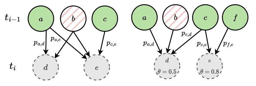
Figure 1. Graphical representation of the IC and WC models (left), and LT model (right). The top row shows activated nodes (green circles) and non-activated nodes (dashed red circles) at timestep $t_{i-1}$. The bottom row shows the nodes that can be activated at timestep $t_{i}$.

3. Related work

We categorize the related works based on how they formulate the IM problem and, in particular, on the objectives they consider, which reflect the same objective functions we consider in our study.

Influence For solving the IM problem, the majority of works builds upon the milestone work (Kempe et al., 2003), which uses a greedy algorithm with approximation guarantees. To reduce the computational cost, several heuristics have been proposed (Leskovec et al., 2007; Chen, Wei and Wang, Yajun and Yang, Siyu, 2009; Jiang, Qingye and Song, Guojie and Gao, Cong and Wang, Yu and Si, Wenjun and Xie, Kunqing, 2011; Wang et al., 2016). A technique based on the statistical estimation of the number of nodes from which the seed set should be sampled has been proposed in (Tang et al., 2015), and then extended to online processing (Tang et al., 2018). As an alternative, various approaches based on EAs emerged (Bucur and Iacca, 2016; Lotf, Jalil Jabari and Azgomi, Mohammad Abdollahi and Dishabi, Mohammad Reza Ebrahimi, 2022; Chawla, Aviral and Cheney, Nick, 2023), which have a computational advantage over the heuristics. The most recent line of works instead focuses on DL approaches, either based on RL (Li et al., 2023; Chen et al., 2023), Learnable Embeddings (Panagopoulos et al., 2020; Ling et al., 2023), or combination of deep RL with EAs (Ma, Lijia and Shao, Zengyang and Li, Xiaocong and Lin, Qiuzhen and Li, Jianqiang and Leung, Victor CM and Nandi, Asoke K, 2022). Of note, all these works only focus on maximizing the influence, fixing a priori the seed set size.

Seed set size Several works proposed to optimize, along with the influence, the seed set size, so to have a min-max IM problem formulation. The earliest works proposed the use of MOEAs (Bucur et al., 2017, 2018; Cunegatti et al., 2022). In (Biswas et al., 2022a), the authors employ a MOEA to optimize seed set size, influence, and budget jointly. Other approaches employ swarm intelligence methods, such as in (Olivares et al., 2021; Riquelme et al., 2023), where the authors employ multi-objective Particle Swarm Optimization (with either scalarization or lexicographic ordering) to maximize the influence while minimizing the seed set size.

Communities This objective aims to fairly distribute the influenced nodes across all the parts (i.e., the communities) of the network. In the literature, some works proposed to combine influence and communities into as single, monotone objective (Tsang et al., 2019; Ali et al., 2023; Rui et al., 2023), while other works focused on Pareto optimization (Gong and Guo, 2023; Feng et al., 2023) or Graph Embeddings (Khajehnejad et al., 2020).

Fairness This objective aims to fairly allocate the nodes in the seed set w.r.t. the network communities they belong to. This objective has been defined in (Stoica et al., 2020; Becker et al., 2022) and handled in various ways, e.g., through multi-objective constrained optimization (Tsang et al., 2019; Razaghi et al., 2022), integer programming (Farnad et al., 2020), and DL (Feng et al., 2023).

Budget The budget, along with the seed set size, is the most studied objective function in IM. The idea behind this objective is that each node in the seed set has a cost (that is usually assumed to be proportional to its out-degree) that needs to be smaller than (or equal to) a fixed value. While this problem could be trivially solved by selecting in the seed set the $k$ nodes with the highest out-degree in the graph, this may represent a sub-optimal solution, depending on the topological structure of the graph at hand. Instead, it is more practical to consider only the sum of the out-degrees of the nodes in the seed set as the actual budget, without imposing any predefined limit on it. Limited budget optimization has been explored in (Bian, Song and Guo, Qintian and Wang, Sibo and Yu, Jeffrey Xu, 2020; Perrault, Pierre and Healey, Jennifer and Wen, Zheng and Valko, Michal, 2020; Pham et al., 2019), while explicit multi-objective settings taking budget into account have been investigated in (Biswas et al., 2022b).

Time As shown in Algorithm 1, the propagation process can stop in two cases: either where no new nodes can be activated anymore, or once a given timestep limit $\tau$ is reached. Using as proxy for the time the number of timesteps of propagation is therefore crucial to reduce the computational cost needed to solve the IM problem. The earliest work that attempted to optimize the propagation time over IM problem relies on a greedy approach (Liu et al., 2012). Later, specific algorithms have been proposed (Chen et al., 2012; Pham et al., 2019) to avoid the complexity of greedy heuristics. The trade-off between influence and time has been empirically analyzed in (Tong et al., 2020), while the relation between fairness and time has been studied in (Ali et al., 2023).

4. Methods

We now introduce the objective functions adopted in the experimentation and the proposed MOEIM algorithm.

4.1. Objective functions

We consider a total of six different objective functions that are specific to the IM problem, namely:

1. Influence ($\mathcal{I}^{\uparrow}$): This refers to the number of nodes in a graph that, starting from a given seed set $S$, are activated throughout the propagation process returned by Algorithm 1. We refer to the set of nodes activated starting from the seed set $S$ as $\sigma(S)$. This function has to be maximized.

2. Seed set size ($\mathcal{S}^{\downarrow}$): This is the number of nodes in the seed set ($|S|$), as given in input to Algorithm 1. This function has to be minimized.

3. Communities: ($\mathcal{C}^{\uparrow}$): For a given set of activated nodes that are not present in the seed set, namely $\sigma(S)\setminus S$, this metric measures the distance between the ideal distribution of activated nodes in each community (i.e., a uniform distribution), and the empirical distribution of activated nodes (Farnad et al., 2020). Throughout this whole work, the communities are referred to as subsets of nodes in a graph that are strongly connected among them while being less connected with the other parts of the graph, and have been computed using the Leiden algorithm (Traag, Vincent A and Waltman, Ludo and Van Eck, Nees Jan, 2019). Since we treat Communities as a problem of matching an empirical distribution of probability with an ideal one, we employ the Jensen-Shannon distance, defined as:

   (1) $$JSD(p,q)=\frac{1}{2}KL(p||M)+\frac{1}{2}KL(q||M)$$

   where $KL$ is the Kullback-Leibler divergence, $p$ and $q$ are the two probability distribution functions, and $M=\frac{(p+q)}{2}$. The Jensen-Shannon divergence is bound in $[0,1]$. As said, in the IM problem one of the probability distributions is fixed (namely, a uniform distribution $\mathcal{U}(1,c)$, where $c$ is the number of communities). Thus, we normalize $JSD$ by dividing it by the maximum $JSD$ distance that can occur in our setup, which is obtained by measuring the distance between a uniform distribution function and the Kronecker’s delta function $\delta$ (which represents the case in which only nodes from a single community are influenced):

   (2) $$JSD_{N}(p,\mathcal{U}(1,c))=\frac{JSD(p,\mathcal{U}(1,c))}{JSD(\delta,\mathcal{U}(1,c))}$$

   In other words, this metric measures if all communities are influenced fairly at the end of the propagation process. This function has to be maximized.

4. Fairness ($\mathcal{F}^{\uparrow}$): Fairness has the same core idea of Communities, i.e., optimizing the nodes’ allocation throughout all the communities. However, differently from the previous metric that is calculated over $\sigma(S)\setminus S$, fairness is measured on the seed set $S$, i.e., it measures if the propagation starts fairly from each community. It is computed exactly as Communities, but on $S$. This function has to be maximized.

5. Budget ($\mathcal{B}^{\downarrow}$): The budget refers to the sum of the out-degrees of the nodes in the selected seed set $S$, i.e., $b=\sum_{n\in S}d_{n}^{out}$. This function has to be minimized.

6. Time ($\mathcal{T}^{\downarrow}$): This is the total propagation time to influence the nodes for which we use, as a proxy, the number of timesteps in the while loop of Algorithm 1. This function is usually referred to as the number of hops of the propagation model. This function has to be minimized.

4.2. MOEIM

Here we present MOEIM, which is composed of three main components, namely: (1) smart initialization (2) many-objective evolutionary optimization, and (3) graph-aware evolutionary operators, described below.

Smart initialization

Each candidate solution represents a possible seed set (i.e., each solution is a set of nodes used as starting points for the propagation process). Practically, each individual consists in a set of integers where each integer is the id of a node used in the seed set. Taking inspiration from (Konotopska, Kateryna and Iacca, Giovanni, 2021), we apply a smart initialization technique that generates an initial population based on the individual capability of each node to influence the network. More specifically, to improve diversity in the initial population, a ratio of $(1-\lambda)$ initial solutions (with $\lambda$ being a hyperparameter) is initialized randomly with a size randomly sampled in $[1,k]$, while a ratio of $\lambda$ is created using the following procedure. First of all, we simulate the influence propagation of each single node for $\tau=3$ hops. Then, we keep the best $k$ nodes (i.e., those that, taken individually, are able to influence the highest number of nodes in the graph), where $k$ is again the maximum size of the individual. Among these $k$ nodes, we filter out those with a out-degree lower than $\Theta$, which is another hyperparameter. Each individual in the $\lambda$ fraction of the initial population is then created with a size randomly sampled in $[1,k]$ by inserting the filtered nodes with probabilities proportional to their out-degree, akin to roulette selection.

Many-objective evolutionary optimization

For the evolutionary optimization core, we rely on the NSGA-II algorithm modified to solve the IM problem as in (Bucur et al., 2018), and made available in (Giovanni Iacca and Kateryna Konotopska and Doina Bucur and Alberto Tonda, 2021). Such an algorithm has been employed due to its ability to seamlessly add new objective functions to the optimization process. However, unlike the existing multi-objective approaches to IM, which as seen earlier employ at most two or three objectives, here we extend the number of objectives up to six. In fact, we study: (1) the case in which we optimize $\mathcal{I}^{\uparrow}$ and $\mathcal{S}^{\downarrow}$ (as in (Bucur et al., 2017, 2018; Cunegatti et al., 2022)); (2) the case in which ($\mathcal{I}^{\uparrow}$-$\mathcal{S}^{\downarrow}$) plus each objective among $\mathcal{C}^{\uparrow}$, $\mathcal{F}^{\uparrow}$, $\mathcal{B}^{\downarrow}$, and $\mathcal{T}^{\downarrow}$ are optimized, resulting in four three-objectives problems; and (3) the case in which we optimize all the metrics from Section 4.1, thus resulting in a six-objectives problem.

Graph-aware evolutionary operators

As demonstrated in previous works (Konotopska, Kateryna and Iacca, Giovanni, 2021; Chawla, Aviral and Cheney, Nick, 2023), while standard one-point crossover is effective for obtaining state-of-the-art performance on the IM problem, graph-aware mutation operators can provide a dramatic performance boost w.r.t. naïve mutations such as random node sampling.

Here, we employ a total of five different mutation operators previously introduced in (Konotopska, Kateryna and Iacca, Giovanni, 2021), of which two are stochastic, while three are graph-aware, to draw a balance between stochasticity and graph-based knowledge. As for the stochastic operators, we use: (1) Global Random Insert Mutation and (2) Global Random Removal Mutation, which respectively randomly adds nodes to the individual, or removes nodes from it. As for the graph-aware operators, we use: (1) Local Neighbor Mutation, where a new node is randomly selected among the neighbors of the node to mutate; (2) Local Neighbor Second-Degree Mutation, which selects a new node in the neighborhood of the nodes to mutate, with probability proportional to its out-degree; (3) Global Low Degree Mutation, where the new node is selected from the whole graph with probability inversely proportional to its out-degree. At each mutation, one of the above mutation operators is selected with uniform probability.

5. Experimental setup

We perform two separate experimental analyses of MOEIM. The first setting [outer color=s1color,fill color=s1color]1 compares our proposed method against two existing heuristics from (Wang et al., 2016; Leskovec et al., 2007) and the state-of-the-art MOEA from (Bucur et al., 2018). The second setting [outer color=s2color,fill color=s2color]2 is focused on comparing the performances of MOEIM w.r.t. a state-of-the-art DL technique, DeepIM (Ling et al., 2023).

Datasets

For the first experimental setting [outer color=s1color,fill color=s1color]1, we selected six different datasets to include directed and undirected, sparse and dense graphs (with an average out-degree from $6$ to $50$), ranging from $\sim$1k to $\sim$9k nodes and $\sim$25k to $\sim$100k edges. We also selected such datasets to cover a broad spectrum of values w.r.t. the number of communities, from $6$ to $46$. The selected datasets are: email-eu-Core^∗ (Leskovec, Jure and Kleinberg, Jon and Faloutsos, Christos, 2007), where nodes represent European research institutions and edges are emails exchanged among them; facebook-combined^∗ (Leskovec, Jure and Mcauley, Julian, 2012), where nodes are Facebook profiles and edges corresponds to friendship among users; gnutella^∗ (Leskovec, Jure and Kleinberg, Jon and Faloutsos, Christos, 2007), which is a peer-to-peer file sharing network; wiki-vote^∗ (Leskovec, Jure and Huttenlocher, Daniel and Kleinberg, Jon, 2010), where nodes corresponds to administrators of Wikipedia and edges corresponds to who-vote-for-whom during an internal election; lastfm^∗ (Benedek Rozemberczki and Rik Sarkar, 2020) is the social network LastFM of Asian users, where nodes are users and edges correspond to mutual following; and Ca-HepTh^∗ (Leskovec, Jure and Kleinberg, Jon and Faloutsos, Christos, 2007) is a collaboration network of High Energy Physics Theory among the arXiv papers of who-cites-whom.

For the second experimental setting [outer color=s2color,fill color=s2color]2, we selected the three publicly available datasets used in (Ling et al., 2023), to allow for a direct comparison with the results presented in the original paper. In particular, the three datasets tested are Jazz^+,- (Gleiser, Pablo M and Danon, Leon, 2003), which is a collaboration network among Jazz musicians/bands, Cora-ML (McCallum et al., 2000), where nodes are Computer Science papers and edges are citations among them, and Power Grid^+,- (Watts, Duncan J and Strogatz, Steven H, 1998), where nodes are power relay points and edges correspond to line connecting them.

For both settings, each dataset has been pre-processed, to remove disconnected components (i.e., portions of the graph disconnected from the largest component of the graph) and low-quality communities. For that, we so relied on the pre-processing approach designed in (Rui et al., 2023), where each final graph represents the largest weakly connected components of the original graph and the communities with less than $10$ nodes are removed. The properties of all datasets, after this pre-processing, are available in Table 1.

Baselines

For the first experimental setting [outer color=s1color,fill color=s1color]1, we selected as baselines two heuristic algorithms, namely Generalized Degree Discount (GDD) (Wang et al., 2016) and Cost-Effective Lazy Forward selection (CELF) (Leskovec et al., 2007). They are both designed to maximize the influence under a constraint on the seed set size, and they both work by adding nodes iteratively until reaching the selected budget. More specifically, GDD adds nodes to the seed set nodes greedily based on the nodes’ out-degree, while CELF is a faster version of the GDD designed to work as a hill-climbing two-pass greedy approach. As a third baseline, we chose the MOEA presented in (Bucur et al., 2018), since it was the first EA proposed for solving the multi-objective IM problem.

For the second experimental setting [outer color=s2color,fill color=s2color]2, we only compare to DeepIM (Ling et al., 2023), since, from the numerical results reported in the original paper, this method outperformed other DL-based approaches when tested on the three selected datasets we tested in our experiments.

Table 1. Tested datasets. Top (bottom) rows: setting [outer color=s1color,fill color=s1color]1 ([outer color=s2color,fill color=s2color]2).

Network Nodes Edges Communities Nodes’ degree Type Num. Min. Max. Avg. Std. Max. email-eu-Core 986 25552 7 57 308 51.83 60.32 546 Directed facebook-combined 4039 88234 17 19 548 43.69 52.41 1045 Undirected gnutella 6299 20776 20 11 753 6.6 8.54 97 Directed wiki-vote 7066 103663 6 29 1959 29.34 60.55 1167 Directed lastfm 7624 27806 23 11 1015 7.29 11.5 216 Undirected CA-HepTh 8638 24827 46 15 625 5.75 6.46 65 Undirected Jazz 198 2742 3 61 73 27.7 17.41 100 Undirected Cora-ML 2810 7981 22 12 441 5.68 8.45 246 Undirected Power Grid 4941 6594 38 31 233 2.67 1.79 19 Undirected

Hyperparameter setting

For the first experimental setting [outer color=s1color,fill color=s1color]1, we set the maximum seed set size to $k=100$ for all the algorithms under comparison, as done in (Bucur et al., 2018). Regarding the time limit ($\tau$), it is worth mentioning that several works (Lee, Jong-Ryul and Chung, Chin-Wan, 2014; Gong, Maoguo and Yan, Jianan and Shen, Bo and Ma, Lijia and Cai, Qing, 2016; Konotopska, Kateryna and Iacca, Giovanni, 2021) empirically showed how setting $\tau$ to a value as low as $2$ (i.e., 2-hop) provides a computationally efficient approximation of influence propagation, yielding final influence values that are practically equivalent to those achieved by CELF. Here, we opt for a value of $\tau=5$ (as (Gong and Guo, 2023)), which provides a fair compromise between the the 2-hop approximation and an unbounded spread process (i.e., $\tau=\infty$). For a fair comparison, such time limit has been applied to all the baselines (GDD, CELF, and MOEA) as well as to MOEIM in the various combinations of objectives (see Section 6.1). In this experimental setting, we use two different propagation models (as in (Bucur et al., 2018; Cunegatti et al., 2022)), namely WC and IC, setting $p=0.05$ in the latter.

For the second experimental setting [outer color=s2color,fill color=s2color]2, for a fair comparison, we relied on the same IM setting adopted in (Ling et al., 2023), where $k$ was set to $20\%$ of nodes in the graph, while no limits on $\tau$ and budget were applied. As in (Ling et al., 2023), in this case we use as propagation models WC and LT, setting the threshold of each node uniformly sampled in $[0.3,0.6]$ in the latter.

For all the experiments, the evolutionary hyperparameters of MOEIM and MOEA (Bucur et al., 2018) have been kept fixed in both experimental settings [outer color=s1color,fill color=s1color]1 and [outer color=s2color,fill color=s2color]2, setting the population size to $100$, the number of offspring to $100$, the number of elites to $2$, the tournament size to $5$ (as in (Cunegatti et al., 2022)), and the number of generations to $100$. For both experimental settings, the fitness evaluation of MOEA and MOEIM solutions have been computed by running 100 Monte Carlo simulations of the tested propagation model. Only for MOEIM the $\lambda=0.33$ of the initial population has been initiated with smart initialization presented in Section 4.2 where $\Theta$ is set to the average out-degree of the graph. The rest of the population is randomly initialized.

Computational setup

To run the experiments, we employed a workstation with an Intel(R) Core(TM) i9-10980XE CPU $@3GHz$ with $18$ cores ($36$ threads) and 125 GB of RAM. Our code is implemented in Python3.8, running in multi-threading.

Table 2. Avg. $\pm$ std. dev. hypervolume ($HV$) achieved by the algorithms under comparison and our proposed MOEIM, across 10 runs for MOEIM, MOEA, and GDD, and (because of computational limits, as discussed in (Bucur et al., 2018)) 3 runs for CELF ($\mathcal{I}^{\uparrow}$: Influence; $\mathcal{S}^{\downarrow}$: Seed set size; $\mathcal{C}^{\uparrow}$: Communities; $\mathcal{F}^{\uparrow}$: Fairness; $\mathcal{B}^{\downarrow}$: Budget; $\mathcal{T}^{\downarrow}$: Time). The column ${HV}_{\textrm{$\mathcal{I}^{\uparrow}$-$\mathcal{S}^{\downarrow}$}}$ indicates the $HV$ in the 2D ($\mathcal{I}^{\uparrow}$-$\mathcal{S}^{\downarrow}$) space, while the next four columns indicate the $HV$ calculated in the corresponding 3D space, and ${HV}_{\textrm{all}}$ indicates the $HV$ calculated in a 6D space in which all objectives ($\mathcal{I}^{\uparrow}$-$\mathcal{S}^{\downarrow}$-$\mathcal{C}^{\uparrow}$-$\mathcal{F}^{\uparrow}$-$\mathcal{B}^{\downarrow}$-$\mathcal{T}^{\downarrow}$) are considered. For MOEIM, we show the case where 2 objectives ($\mathcal{I}^{\uparrow}$-$\mathcal{S}^{\downarrow}$), the combinations of 3 objectives ($\mathcal{I}^{\uparrow}$-$\mathcal{S}^{\downarrow}$ plus either $\mathcal{C}^{\uparrow}$, $\mathcal{F}^{\uparrow}$, $\mathcal{B}^{\downarrow}$ or $\mathcal{S}^{\downarrow}$), and all objectives ($\mathcal{I}^{\uparrow}$-$\mathcal{S}^{\downarrow}$-$\mathcal{C}^{\uparrow}$-$\mathcal{F}^{\uparrow}$-$\mathcal{B}^{\downarrow}$-$\mathcal{T}^{\downarrow}$) are considered during the evolutionary process. The colored (underlined) cells indicate the highest (second highest) value per column, separately per each dataset, propagation model, and combination of objectives considered to calculate the $HV$.

Algorithm Independent Cascade (IC) Weighted Cascade (WC) ${HV}_{\textrm{$\mathcal{I}^{\uparrow}$-$\mathcal{S}^{\downarrow}$}}$ ${HV}_{\textrm{$\mathcal{I}^{\uparrow}$-$\mathcal{S}^{\downarrow}$-$\mathcal{C}^{\uparrow}$}}$ ${HV}_{\textrm{$\mathcal{I}^{\uparrow}$-$\mathcal{S}^{\downarrow}$-$\mathcal{F}^{\uparrow}$}}$ ${HV}_{\textrm{$\mathcal{I}^{\uparrow}$-$\mathcal{S}^{\downarrow}$-$\mathcal{B}^{\downarrow}$}}$ ${HV}_{\textrm{$\mathcal{I}^{\uparrow}$-$\mathcal{S}^{\downarrow}$-$\mathcal{T}^{\downarrow}$}}$ ${HV}_{\textrm{all}}$ ${HV}_{\textrm{$\mathcal{I}^{\uparrow}$-$\mathcal{S}^{\downarrow}$}}$ ${HV}_{\textrm{$\mathcal{I}^{\uparrow}$-$\mathcal{S}^{\downarrow}$-$\mathcal{C}^{\uparrow}$}}$ ${HV}_{\textrm{$\mathcal{I}^{\uparrow}$-$\mathcal{S}^{\downarrow}$-$\mathcal{F}^{\uparrow}$}}$ ${HV}_{\textrm{$\mathcal{I}^{\uparrow}$-$\mathcal{S}^{\downarrow}$-$\mathcal{B}^{\downarrow}$}}$ ${HV}_{\textrm{$\mathcal{I}^{\uparrow}$-$\mathcal{S}^{\downarrow}$-$\mathcal{T}^{\downarrow}$}}$ ${HV}_{\textrm{all}}$ email-eu-Core GDD (Wang et al., 2016) $4.90{\textrm{e}}{-1}\pm 3.72{\textrm{e}}{-5}$ $4.62{\textrm{e}}{-1}\pm 2.29{\textrm{e}}{-4}$ $4.19{\textrm{e}}{-1}\pm 3.82{\textrm{e}}{-6}$ $4.57{\textrm{e}}{-1}\pm 8.45{\textrm{e}}{-5}$ $6.18{\textrm{e}}{-2}\pm 3.62{\textrm{e}}{-3}$ $3.21{\textrm{e}}{-2}\pm 2.94{\textrm{e}}{-3}$ $4.11{\textrm{e}}{-1}\pm 2.26{\textrm{e}}{-4}$ $3.78{\textrm{e}}{-1}\pm 7.52{\textrm{e}}{-5}$ $3.01{\textrm{e}}{-1}\pm 1.21{\textrm{e}}{-4}$ $\mathbf{3.10{\textrm{e}}{-1}\pm 4.47{\textrm{e}}{-4}}$ $7.45{\textrm{e}}{-2}\pm 5.62{\textrm{e}}{-3}$ $2.68{\textrm{e}}{-2}\pm 4.93{\textrm{e}}{-3}$ CELF (Leskovec et al., 2007) $4.87{\textrm{e}}{-1}\pm 8.97{\textrm{e}}{-4}$ $4.58{\textrm{e}}{-1}\pm 7.86{\textrm{e}}{-4}$ $4.00{\textrm{e}}{-1}\pm 3.54{\textrm{e}}{-3}$ $4.60{\textrm{e}}{-1}\pm 1.12{\textrm{e}}{-3}$ $2.52{\textrm{e}}{-2}\pm 1.43{\textrm{e}}{-2}$ $1.43{\textrm{e}}{-2}\pm 1.05{\textrm{e}}{-2}$ $3.80{\textrm{e}}{-1}\pm 1.40{\textrm{e}}{-3}$ $3.47{\textrm{e}}{-1}\pm 1.49{\textrm{e}}{-3}$ $3.17{\textrm{e}}{-1}\pm 6.99{\textrm{e}}{-3}$ $3.07{\textrm{e}}{-1}\pm 1.32{\textrm{e}}{-3}$ $7.01{\textrm{e}}{-2}\pm 1.62{\textrm{e}}{-3}$ $3.59{\textrm{e}}{-2}\pm 3.62{\textrm{e}}{-3}$ MOEA (Bucur et al., 2018) $4.96{\textrm{e}}{-1}\pm 1.84{\textrm{e}}{-3}$ $4.68{\textrm{e}}{-1}\pm 1.80{\textrm{e}}{-3}$ $4.17{\textrm{e}}{-1}\pm 1.39{\textrm{e}}{-2}$ $4.53{\textrm{e}}{-1}\pm 2.14{\textrm{e}}{-3}$ $1.97{\textrm{e}}{-2}\pm 2.79{\textrm{e}}{-2}$ $3.00{\textrm{e}}{-3}\pm 9.49{\textrm{e}}{-3}$ $3.59{\textrm{e}}{-1}\pm 6.48{\textrm{e}}{-3}$ $3.26{\textrm{e}}{-1}\pm 6.57{\textrm{e}}{-3}$ $3.15{\textrm{e}}{-1}\pm 7.68{\textrm{e}}{-3}$ $2.53{\textrm{e}}{-1}\pm 1.84{\textrm{e}}{-3}$ $4.97{\textrm{e}}{-2}\pm 5.22{\textrm{e}}{-3}$ $2.11{\textrm{e}}{-2}\pm 5.25{\textrm{e}}{-3}$ MOEIM ($\mathcal{I}^{\uparrow}$-$\mathcal{S}^{\downarrow}$) $\mathbf{4.99{\textrm{e}}{-1}\pm 5.99{\textrm{e}}{-4}}$ $4.70{\textrm{e}}{-1}\pm 5.59{\textrm{e}}{-4}$ $4.18{\textrm{e}}{-1}\pm 4.33{\textrm{e}}{-3}$ $4.54{\textrm{e}}{-1}\pm 3.18{\textrm{e}}{-3}$ $0.00{\textrm{e}}{0}\pm 0.00{\textrm{e}}{0}$ $3.43{\textrm{e}}{-4}\pm 1.08{\textrm{e}}{-3}$ $\mathbf{4.13{\textrm{e}}{-1}\pm 1.37{\textrm{e}}{-3}}$ $\mathbf{3.82{\textrm{e}}{-1}\pm 1.30{\textrm{e}}{-3}}$ $3.52{\textrm{e}}{-1}\pm 1.63{\textrm{e}}{-2}$ $2.56{\textrm{e}}{-1}\pm 3.49{\textrm{e}}{-4}$ $7.06{\textrm{e}}{-2}\pm 5.46{\textrm{e}}{-3}$ $1.67{\textrm{e}}{-2}\pm 6.13{\textrm{e}}{-3}$ MOEIM ($\mathcal{I}^{\uparrow}$-$\mathcal{S}^{\downarrow}$-$\mathcal{C}^{\uparrow}$) $4.95{\textrm{e}}{-1}\pm 1.68{\textrm{e}}{-3}$ $\mathbf{4.72{\textrm{e}}{-1}\pm 1.53{\textrm{e}}{-3}}$ $4.17{\textrm{e}}{-1}\pm 5.05{\textrm{e}}{-3}$ $4.54{\textrm{e}}{-1}\pm 1.17{\textrm{e}}{-3}$ $1.92{\textrm{e}}{-2}\pm 2.49{\textrm{e}}{-2}$ $3.08{\textrm{e}}{-3}\pm 4.51{\textrm{e}}{-3}$ $4.09{\textrm{e}}{-1}\pm 1.20{\textrm{e}}{-3}$ $3.80{\textrm{e}}{-1}\pm 1.20{\textrm{e}}{-3}$ $3.76{\textrm{e}}{-1}\pm 2.09{\textrm{e}}{-3}$ $2.57{\textrm{e}}{-1}\pm 8.29{\textrm{e}}{-4}$ $7.98{\textrm{e}}{-2}\pm 4.57{\textrm{e}}{-3}$ $2.76{\textrm{e}}{-2}\pm 4.99{\textrm{e}}{-3}$ MOEIM ($\mathcal{I}^{\uparrow}$-$\mathcal{S}^{\downarrow}$-$\mathcal{F}^{\uparrow}$) $4.95{\textrm{e}}{-1}\pm 6.50{\textrm{e}}{-4}$ $4.67{\textrm{e}}{-1}\pm 8.70{\textrm{e}}{-4}$ $\mathbf{4.64{\textrm{e}}{-1}\pm 1.48{\textrm{e}}{-3}}$ $4.55{\textrm{e}}{-1}\pm 2.05{\textrm{e}}{-3}$ $5.67{\textrm{e}}{-3}\pm 4.11{\textrm{e}}{-3}$ $2.31{\textrm{e}}{-3}\pm 5.26{\textrm{e}}{-3}$ $4.06{\textrm{e}}{-1}\pm 1.39{\textrm{e}}{-3}$ $2.11{\textrm{e}}{-1}\pm 1.98{\textrm{e}}{-3}$ $\mathbf{3.89{\textrm{e}}{-1}\pm 1.28{\textrm{e}}{-3}}$ $2.60{\textrm{e}}{-1}\pm 1.79{\textrm{e}}{-3}$ $7.61{\textrm{e}}{-2}\pm 2.28{\textrm{e}}{-3}$ $3.40{\textrm{e}}{-2}\pm 4.03{\textrm{e}}{-3}$ MOEIM ($\mathcal{I}^{\uparrow}$-$\mathcal{S}^{\downarrow}$-$\mathcal{B}^{\downarrow}$) $4.91{\textrm{e}}{-1}\pm 1.82{\textrm{e}}{-3}$ $4.63{\textrm{e}}{-1}\pm 1.83{\textrm{e}}{-3}$ $4.41{\textrm{e}}{-1}\pm 4.35{\textrm{e}}{-3}$ $\mathbf{4.74{\textrm{e}}{-1}\pm 1.70{\textrm{e}}{-3}}$ $1.38{\textrm{e}}{-1}\pm 2.81{\textrm{e}}{-3}$ $3.45{\textrm{e}}{-2}\pm 6.53{\textrm{e}}{-3}$ $3.94{\textrm{e}}{-1}\pm 9.16{\textrm{e}}{-4}$ $3.63{\textrm{e}}{-1}\pm 6.83{\textrm{e}}{-4}$ $3.61{\textrm{e}}{-1}\pm 2.82{\textrm{e}}{-3}$ $2.66{\textrm{e}}{-1}\pm 1.16{\textrm{e}}{-3}$ $8.83{\textrm{e}}{-2}\pm 6.41{\textrm{e}}{-4}$ $3.97{\textrm{e}}{-2}\pm 1.45{\textrm{e}}{-3}$ MOEIM ($\mathcal{I}^{\uparrow}$-$\mathcal{S}^{\downarrow}$-$\mathcal{T}^{\downarrow}$) $4.98{\textrm{e}}{-1}\pm 6.78{\textrm{e}}{-4}$ $4.69{\textrm{e}}{-1}\pm 5.90{\textrm{e}}{-4}$ $4.22{\textrm{e}}{-1}\pm 8.15{\textrm{e}}{-3}$ $4.64{\textrm{e}}{-1}\pm 3.29{\textrm{e}}{-4}$ $1.60{\textrm{e}}{-1}\pm 5.66{\textrm{e}}{-3}$ $4.37{\textrm{e}}{-2}\pm,3.57{\textrm{e}}{-3}$ $4.10{\textrm{e}}{-1}\pm 7.90{\textrm{e}}{-4}$ $3.79{\textrm{e}}{-1}\pm 7.93{\textrm{e}}{-4}$ $3.61{\textrm{e}}{-1}\pm 5.18{\textrm{e}}{-3}$ $2.59{\textrm{e}}{-1}\pm 1.23{\textrm{e}}{-3}$ $\mathbf{9.44{\textrm{e}}{-2}\pm 7.78{\textrm{e}}{-4}}$ $3.56{\textrm{e}}{-2}\pm 8.13{\textrm{e}}{-4}$ MOEIM (all) $4.86{\textrm{e}}{-1}\pm 5.43{\textrm{e}}{-4}$ $4.61{\textrm{e}}{-1}\pm 6.62{\textrm{e}}{-4}$ $4.46{\textrm{e}}{-1}\pm 2.55{\textrm{e}}{-3}$ $4.66{\textrm{e}}{-1}\pm 8.19{\textrm{e}}{-4}$ $\mathbf{1.60{\textrm{e}}{-1}\pm 1.30{\textrm{e}}{-3}}$ $\pagecolor{red!70}\mathbf{7.29{\textrm{e}}{-2}\pm 3.77{\textrm{e}}{-3}}$ $3.81{\textrm{e}}{-1}\pm 2.42{\textrm{e}}{-3}$ $3.50{\textrm{e}}{-1}\pm 2.35{\textrm{e}}{-3}$ $3.57{\textrm{e}}{-1}\pm 1.36{\textrm{e}}{-3}$ $2.55{\textrm{e}}{-1}\pm 8.23{\textrm{e}}{-4}$ $8.99{\textrm{e}}{-2}\pm 4.20{\textrm{e}}{-4}$ $\pagecolor{red!70}\mathbf{4.25{\textrm{e}}{-2}\pm 7.43{\textrm{e}}{-4}}$ facebook-combined GDD (Wang et al., 2016) $5.15{\textrm{e}}{-1}\pm 4.22{\textrm{e}}{-5}$ $3.65{\textrm{e}}{-1}\pm 4.30{\textrm{e}}{-4}$ $2.95{\textrm{e}}{-1}\pm 2.38{\textrm{e}}{-5}$ $4.62{\textrm{e}}{-1}\pm 2.92{\textrm{e}}{-4}$ $0.00{\textrm{e}}{0}\pm 0.00{\textrm{e}}{0}$ $0.00{\textrm{e}}{0}\pm 0.00{\textrm{e}}{0}$ $2.07{\textrm{e}}{-1}\pm 9.42{\textrm{e}}{-5}$ $1.34{\textrm{e}}{-1}\pm 4.89{\textrm{e}}{-5}$ $8.76{\textrm{e}}{-2}\pm 3.38{\textrm{e}}{-5}$ $1.70{\textrm{e}}{-1}\pm 5.91{\textrm{e}}{-5}$ $4.66{\textrm{e}}{-3}\pm 3.30{\textrm{e}}{-3}$ $1.81{\textrm{e}}{-4}\pm 1.91{\textrm{e}}{-4}$ CELF (Leskovec et al., 2007) $5.18{\textrm{e}}{-1}\pm 4.99{\textrm{e}}{-4}$ $3.65{\textrm{e}}{-1}\pm 1.08{\textrm{e}}{-3}$ $2.84{\textrm{e}}{-1}\pm 9.19{\textrm{e}}{-3}$ $4.73{\textrm{e}}{-1}\pm 1.64{\textrm{e}}{-3}$ $0.00{\textrm{e}}{0}\pm 0.00{\textrm{e}}{0}$ $0.00{\textrm{e}}{0}\pm 0.00{\textrm{e}}{0}$ $2.46{\textrm{e}}{-1}\pm 1.10{\textrm{e}}{-3}$ $1.84{\textrm{e}}{-1}\pm 7.23{\textrm{e}}{-4}$ $1.37{\textrm{e}}{-1}\pm 3.06{\textrm{e}}{-3}$ $2.04{\textrm{e}}{-1}\pm 6.49{\textrm{e}}{-4}$ $2.33{\textrm{e}}{-3}\pm 3.29{\textrm{e}}{-3}$ $1.18{\textrm{e}}{-4}\pm 2.05{\textrm{e}}{-4}$ MOEA (Bucur et al., 2018) $5.02{\textrm{e}}{-1}\pm 4.35{\textrm{e}}{-3}$ $3.47{\textrm{e}}{-1}\pm 5.72{\textrm{e}}{-3}$ $2.98{\textrm{e}}{-1}\pm 5.97{\textrm{e}}{-3}$ $4.74{\textrm{e}}{-1}\pm 1.52{\textrm{e}}{-3}$ $0.00{\textrm{e}}{0}\pm 0.00{\textrm{e}}{0}$ $0.00{\textrm{e}}{0}\pm 0.00{\textrm{e}}{0}$ $1.96{\textrm{e}}{-1}\pm 5.32{\textrm{e}}{-3}$ $1.32{\textrm{e}}{-1}\pm 7.79{\textrm{e}}{-3}$ $1.21{\textrm{e}}{-1}\pm 6.25{\textrm{e}}{-3}$ $1.71{\textrm{e}}{-1}\pm 3.28{\textrm{e}}{-3}$ $0.00{\textrm{e}}{0}\pm 0.00{\textrm{e}}{0}$ $1.25{\textrm{e}}{-4}\pm 1.49{\textrm{e}}{-4}$ MOEIM ($\mathcal{I}^{\uparrow}$-$\mathcal{S}^{\downarrow}$) $\mathbf{5.22{\textrm{e}}{-1}\pm 8.53{\textrm{e}}{-4}}$ $\underline{3.78{\textrm{e}}{-1}\pm 5.26{\textrm{e}}{-3}}$ $3.18{\textrm{e}}{-1}\pm 5.60{\textrm{e}}{-3}$ $4.80{\textrm{e}}{-1}\pm 4.06{\textrm{e}}{-3}$ $0.00{\textrm{e}}{0}\pm 0.00{\textrm{e}}{0}$ $0.00{\textrm{e}}{0}\pm 0.00{\textrm{e}}{0}$ $\mathbf{2.50{\textrm{e}}{-1}\pm 2.78{\textrm{e}}{-4}}$ $1.89{\textrm{e}}{-1}\pm 9.27{\textrm{e}}{-4}$ $1.49{\textrm{e}}{-1}\pm 9.40{\textrm{e}}{-4}$ $2.06{\textrm{e}}{-1}\pm 1.25{\textrm{e}}{-3}$ $8.34{\textrm{e}}{-3}\pm 3.15{\textrm{e}}{-3}$ $2.56{\textrm{e}}{-4}\pm 2.42{\textrm{e}}{-4}$ MOEIM ($\mathcal{I}^{\uparrow}$-$\mathcal{S}^{\downarrow}$-$\mathcal{C}^{\uparrow}$) $5.19{\textrm{e}}{-1}\pm 1.03{\textrm{e}}{-3}$ $\mathbf{3.93{\textrm{e}}{-1}\pm 1.88{\textrm{e}}{-3}}$ $3.10{\textrm{e}}{-1}\pm 9.67{\textrm{e}}{-3}$ $4.78{\textrm{e}}{-1}\pm 1.31{\textrm{e}}{-3}$ $0.00{\textrm{e}}{0}\pm 0.00{\textrm{e}}{0}$ $1.58{\textrm{e}}{-4}\pm 5.01{\textrm{e}}{-4}$ $2.46{\textrm{e}}{-1}\pm 1.15{\textrm{e}}{-3}$ $\mathbf{1.95{\textrm{e}}{-1}\pm 8.70{\textrm{e}}{-4}}$ $1.65{\textrm{e}}{-1}\pm 3.67{\textrm{e}}{-3}$ $2.04{\textrm{e}}{-1}\pm 1.37{\textrm{e}}{-3}$ $4.09{\textrm{e}}{-3}\pm 2.98{\textrm{e}}{-3}$ $1.97{\textrm{e}}{-4}\pm 2.19{\textrm{e}}{-4}$ MOEIM ($\mathcal{I}^{\uparrow}$-$\mathcal{S}^{\downarrow}$-$\mathcal{F}^{\uparrow}$) $5.14{\textrm{e}}{-1}\pm 1.38{\textrm{e}}{-3}$ $3.71{\textrm{e}}{-1}\pm 4.36{\textrm{e}}{-4}$ $\mathbf{3.73{\textrm{e}}{-1}\pm 2.11{\textrm{e}}{-3}}$ $\underline{4.86{\textrm{e}}{-1}\pm 3.54{\textrm{e}}{-3}}$ $3.18{\textrm{e}}{-3}\pm 4.49{\textrm{e}}{-3}$ $1.13{\textrm{e}}{-4}\pm 2.39{\textrm{e}}{-4}$ $2.41{\textrm{e}}{-1}\pm 1.75{\textrm{e}}{-3}$ $1.87{\textrm{e}}{-1}\pm 2.13{\textrm{e}}{-3}$ $\mathbf{1.79{\textrm{e}}{-1}\pm 1.40{\textrm{e}}{-3}}$ $2.02{\textrm{e}}{-1}\pm 1.22{\textrm{e}}{-3}$ $8.46{\textrm{e}}{-3}\pm 2.61{\textrm{e}}{-3}$ $6.99{\textrm{e}}{-4}\pm 6.83{\textrm{e}}{-4}$ MOEIM ($\mathcal{I}^{\uparrow}$-$\mathcal{S}^{\downarrow}$-$\mathcal{B}^{\downarrow}$) $5.03{\textrm{e}}{-1}\pm 1.40{\textrm{e}}{-3}$ $3.54{\textrm{e}}{-1}\pm 2.86{\textrm{e}}{-3}$ $3.28{\textrm{e}}{-1}\pm 6.31{\textrm{e}}{-4}$ $\mathbf{4.91{\textrm{e}}{-1}\pm 1.28{\textrm{e}}{-3}}$ $\mathbf{7.66{\textrm{e}}{-2}\pm 4.09{\textrm{e}}{-3}}$ $6.72{\textrm{e}}{-3}\pm 1.52{\textrm{e}}{-3}$ $2.41{\textrm{e}}{-1}\pm 2.13{\textrm{e}}{-3}$ $1.80{\textrm{e}}{-1}\pm 2.15{\textrm{e}}{-3}$ $1.48{\textrm{e}}{-1}\pm 2.27{\textrm{e}}{-3}$ $\mathbf{2.07{\textrm{e}}{-1}\pm 1.47{\textrm{e}}{-3}}$ $1.70{\textrm{e}}{-2}\pm 1.75{\textrm{e}}{-3}$ $2.12{\textrm{e}}{-3}\pm 6.82{\textrm{e}}{-4}$ MOEIM ($\mathcal{I}^{\uparrow}$-$\mathcal{S}^{\downarrow}$-$\mathcal{T}^{\downarrow}$) $5.21{\textrm{e}}{-1}\pm 3.96{\textrm{e}}{-4}$ $3.70{\textrm{e}}{-1}\pm 3.58{\textrm{e}}{-3}$ $3.11{\textrm{e}}{-1}\pm 1.25{\textrm{e}}{-2}$ $4.82{\textrm{e}}{-1}\pm 5.86{\textrm{e}}{-4}$ $7.59{\textrm{e}}{-2}\pm 2.84{\textrm{e}}{-3}$ $5.86{\textrm{e}}{-3}\pm 1.25{\textrm{e}}{-3}$ $2.48{\textrm{e}}{-1}\pm 7.09{\textrm{e}}{-4}$ $1.88{\textrm{e}}{-1}\pm 1.06{\textrm{e}}{-3}$ $1.51{\textrm{e}}{-1}\pm 2.52{\textrm{e}}{-3}$ $2.06{\textrm{e}}{-1}\pm 4.93{\textrm{e}}{-4}$ $\mathbf{1.85{\textrm{e}}{-2}\pm 1.55{\textrm{e}}{-3}}$ $2.20{\textrm{e}}{-3}\pm 3.36{\textrm{e}}{-4}$ MOEIM (all) $4.91{\textrm{e}}{-1}\pm 1.66{\textrm{e}}{-3}$ $3.53{\textrm{e}}{-1}\pm 3.71{\textrm{e}}{-3}$ $\underline{3.50{\textrm{e}}{-1}\pm 1.44{\textrm{e}}{-3}}$ $4.78{\textrm{e}}{-1}\pm 1.31{\textrm{e}}{-3}$ $6.40{\textrm{e}}{-2}\pm 2.02{\textrm{e}}{-3}$ $\pagecolor{red!70}\mathbf{9.22{\textrm{e}}{-3}\pm 1.01{\textrm{e}}{-3}}$ $2.22{\textrm{e}}{-1}\pm 4.23{\textrm{e}}{-3}$ $1.66{\textrm{e}}{-1}\pm 3.35{\textrm{e}}{-3}$ $1.60{\textrm{e}}{-1}\pm 2.19{\textrm{e}}{-3}$ $1.88{\textrm{e}}{-1}\pm 3.00{\textrm{e}}{-3}$ $1.61{\textrm{e}}{-2}\pm 3.21{\textrm{e}}{-4}$ $\pagecolor{red!70}\mathbf{3.89{\textrm{e}}{-3}\pm 3.53{\textrm{e}}{-4}}$ gnutella GDD (Wang et al., 2016) $\pagecolor{blue!70}1.55{\textrm{e}}{-2}\pm 7.03{\textrm{e}}{-6}$ $\pagecolor{green!80}\mathbf{1.01{\textrm{e}}{-2}\pm 9.04{\textrm{e}}{-6}}$ $9.90{\textrm{e}}{-3}\pm 3.79{\textrm{e}}{-6}$ $9.06{\textrm{e}}{-3}\pm 7.26{\textrm{e}}{-6}$ $9.75{\textrm{e}}{-3}\pm 1.46{\textrm{e}}{-4}$ $1.84{\textrm{e}}{-3}\pm 1.63{\textrm{e}}{-5}$ $1.64{\textrm{e}}{-1}\pm 1.64{\textrm{e}}{-4}$ $1.43{\textrm{e}}{-1}\pm 1.30{\textrm{e}}{-4}$ $1.04{\textrm{e}}{-1}\pm 1.07{\textrm{e}}{-4}$ $1.09{\textrm{e}}{-1}\pm 1.51{\textrm{e}}{-4}$ $6.95{\textrm{e}}{-3}\pm 2.25{\textrm{e}}{-3}$ $1.23{\textrm{e}}{-3}\pm 6.39{\textrm{e}}{-4}$ CELF (Leskovec et al., 2007) $1.53{\textrm{e}}{-2}\pm 1.11{\textrm{e}}{-4}$ $8.34{\textrm{e}}{-3}\pm 1.71{\textrm{e}}{-4}$ $7.81{\textrm{e}}{-3}\pm 4.94{\textrm{e}}{-4}$ $9.48{\textrm{e}}{-3}\pm 3.19{\textrm{e}}{-5}$ $8.58{\textrm{e}}{-3}\pm 1.65{\textrm{e}}{-4}$ $1.33{\textrm{e}}{-3}\pm 1.56{\textrm{e}}{-4}$ $\mathbf{2.93{\textrm{e}}{-1}\pm 2.29{\textrm{e}}{-3}}$ $\mathbf{2.68{\textrm{e}}{-1}\pm 2.68{\textrm{e}}{-3}}$ $1.93{\textrm{e}}{-1}\pm 4.30{\textrm{e}}{-3}$ $\mathbf{2.30{\textrm{e}}{-1}\pm 1.69{\textrm{e}}{-3}}$ $3.63{\textrm{e}}{-3}\pm 3.76{\textrm{e}}{-5}$ $3.67{\textrm{e}}{-4}\pm 1.43{\textrm{e}}{-6}$ MOEA (Bucur et al., 2018) $1.34{\textrm{e}}{-2}\pm 1.55{\textrm{e}}{-4}$ $7.48{\textrm{e}}{-3}\pm 2.36{\textrm{e}}{-4}$ $9.33{\textrm{e}}{-3}\pm 9.90{\textrm{e}}{-5}$ $8.58{\textrm{e}}{-3}\pm 6.39{\textrm{e}}{-5}$ $8.51{\textrm{e}}{-3}\pm 8.23{\textrm{e}}{-5}$ $1.70{\textrm{e}}{-3}\pm 7.55{\textrm{e}}{-5}$ $1.86{\textrm{e}}{-1}\pm 5.41{\textrm{e}}{-3}$ $1.64{\textrm{e}}{-1}\pm 5.68{\textrm{e}}{-3}$ $1.22{\textrm{e}}{-1}\pm 4.75{\textrm{e}}{-3}$ $1.57{\textrm{e}}{-1}\pm 5.12{\textrm{e}}{-3}$ $1.93{\textrm{e}}{-3}\pm 1.39{\textrm{e}}{-3}$ $1.92{\textrm{e}}{-4}\pm 2.06{\textrm{e}}{-4}$ MOEIM ($\mathcal{I}^{\uparrow}$-$\mathcal{S}^{\downarrow}$) $1.55{\textrm{e}}{-2}\pm 1.22{\textrm{e}}{-4}$ $9.54{\textrm{e}}{-3}\pm 1.43{\textrm{e}}{-4}$ $1.06{\textrm{e}}{-2}\pm 2.45{\textrm{e}}{-4}$ $8.34{\textrm{e}}{-3}\pm 3.02{\textrm{e}}{-5}$ $9.06{\textrm{e}}{-3}\pm 1.38{\textrm{e}}{-4}$ $1.61{\textrm{e}}{-3}\pm 7.57{\textrm{e}}{-5}$ $2.90{\textrm{e}}{-1}\pm 1.26{\textrm{e}}{-3}$ $2.66{\textrm{e}}{-1}\pm 9.10{\textrm{e}}{-4}$ $2.08{\textrm{e}}{-1}\pm 1.24{\textrm{e}}{-3}$ $2.06{\textrm{e}}{-1}\pm 2.21{\textrm{e}}{-3}$ $2.83{\textrm{e}}{-3}\pm 6.74{\textrm{e}}{-4}$ $2.22{\textrm{e}}{-4}\pm 1.38{\textrm{e}}{-4}$ MOEIM ($\mathcal{I}^{\uparrow}$-$\mathcal{S}^{\downarrow}$-$\mathcal{C}^{\uparrow}$) $1.52{\textrm{e}}{-2}\pm 9.41{\textrm{e}}{-5}$ $9.73{\textrm{e}}{-3}\pm 1.18{\textrm{e}}{-4}$ $1.18{\textrm{e}}{-2}\pm 2.29{\textrm{e}}{-4}$ $8.28{\textrm{e}}{-3}\pm 6.27{\textrm{e}}{-5}$ $9.50{\textrm{e}}{-3}\pm 2.05{\textrm{e}}{-4}$ $2.02{\textrm{e}}{-3}\pm 1.06{\textrm{e}}{-4}$ $2.80{\textrm{e}}{-1}\pm 3.58{\textrm{e}}{-3}$ $2.61{\textrm{e}}{-1}\pm 3.37{\textrm{e}}{-3}$ $2.07{\textrm{e}}{-1}\pm 6.51{\textrm{e}}{-3}$ $2.00{\textrm{e}}{-1}\pm 3.09{\textrm{e}}{-3}$ $0.00{\textrm{e}}{0}\pm 0.00{\textrm{e}}{0}$ $3.46{\textrm{e}}{-4}\pm 2.95{\textrm{e}}{-4}$ MOEIM ($\mathcal{I}^{\uparrow}$-$\mathcal{S}^{\downarrow}$-$\mathcal{F}^{\uparrow}$) $1.43{\textrm{e}}{-2}\pm 7.34{\textrm{e}}{-5}$ $8.75{\textrm{e}}{-3}\pm 8.07{\textrm{e}}{-5}$ $\pagecolor{green!80}\mathbf{1.23{\textrm{e}}{-2}\pm 1.55{\textrm{e}}{-4}}$ $8.57{\textrm{e}}{-3}\pm 3.50{\textrm{e}}{-4}$ $9.37{\textrm{e}}{-3}\pm 9.72{\textrm{e}}{-5}$ $2.47{\textrm{e}}{-3}\pm 1.16{\textrm{e}}{-4}$ $2.71{\textrm{e}}{-1}\pm 1.58{\textrm{e}}{-3}$ $2.49{\textrm{e}}{-1}\pm 1.53{\textrm{e}}{-3}$ $\mathbf{2.33{\textrm{e}}{-1}\pm 4.13{\textrm{e}}{-3}}$ $1.90{\textrm{e}}{-1}\pm 1.83{\textrm{e}}{-3}$ $6.40{\textrm{e}}{-3}\pm 2.02{\textrm{e}}{-3}$ $8.61{\textrm{e}}{-4}\pm 3.24{\textrm{e}}{-4}$ MOEIM ($\mathcal{I}^{\uparrow}$-$\mathcal{S}^{\downarrow}$-$\mathcal{B}^{\downarrow}$) $1.43{\textrm{e}}{-2}\pm 8.04{\textrm{e}}{-5}$ $8.52{\textrm{e}}{-3}\pm 1.50{\textrm{e}}{-4}$ $1.11{\textrm{e}}{-2}\pm 2.64{\textrm{e}}{-4}$ $\pagecolor{green!80}\mathbf{1.05{\textrm{e}}{-2}\pm 6.82{\textrm{e}}{-5}}$ $1.04{\textrm{e}}{-2}\pm 3.95{\textrm{e}}{-4}$ $2.75{\textrm{e}}{-3}\pm 1.08{\textrm{e}}{-4}$ $2.82{\textrm{e}}{-1}\pm 1.56{\textrm{e}}{-3}$ $2.59{\textrm{e}}{-1}\pm 8.24{\textrm{e}}{-4}$ $2.12{\textrm{e}}{-1}\pm 1.37{\textrm{e}}{-3}$ $2.19{\textrm{e}}{-1}\pm 2.68{\textrm{e}}{-3}$ $3.98{\textrm{e}}{-3}\pm 7.49{\textrm{e}}{-4}$ $4.47{\textrm{e}}{-4}\pm 1.46{\textrm{e}}{-4}$ MOEIM ($\mathcal{I}^{\uparrow}$-$\mathcal{S}^{\downarrow}$-$\mathcal{T}^{\downarrow}$) $1.52{\textrm{e}}{-2}\pm 2.64{\textrm{e}}{-4}$ $9.27{\textrm{e}}{-3}\pm 3.50{\textrm{e}}{-4}$ $1.08{\textrm{e}}{-2}\pm 4.58{\textrm{e}}{-4}$ $9.27{\textrm{e}}{-3}\pm 9.49{\textrm{e}}{-5}$ $\pagecolor{green!80}\mathbf{1.14{\textrm{e}}{-2}\pm 1.94{\textrm{e}}{-4}}$ $2.26{\textrm{e}}{-3}\pm 1.19{\textrm{e}}{-4}$ $2.81{\textrm{e}}{-1}\pm 2.54{\textrm{e}}{-3}$ $2.57{\textrm{e}}{-1}\pm 2.44{\textrm{e}}{-3}$ $2.01{\textrm{e}}{-1}\pm 4.29{\textrm{e}}{-3}$ $1.98{\textrm{e}}{-1}\pm 2.72{\textrm{e}}{-3}$ $\mathbf{1.74{\textrm{e}}{-2}\pm 1.26{\textrm{e}}{-3}}$ $4.28{\textrm{e}}{-3}\pm 8.34{\textrm{e}}{-4}$ MOEIM (all) $1.36{\textrm{e}}{-2}\pm 4.89{\textrm{e}}{-5}$ $7.86{\textrm{e}}{-3}\pm 8.30{\textrm{e}}{-5}$ $1.11{\textrm{e}}{-2}\pm 1.81{\textrm{e}}{-4}$ $1.01{\textrm{e}}{-2}\pm 2.77{\textrm{e}}{-5}$ $1.05{\textrm{e}}{-2}\pm 1.65{\textrm{e}}{-4}$ $\pagecolor{red!70}\mathbf{2.81{\textrm{e}}{-3}\pm 5.96{\textrm{e}}{-5}}$ $2.46{\textrm{e}}{-1}\pm 1.92{\textrm{e}}{-3}$ $2.26{\textrm{e}}{-1}\pm 2.33{\textrm{e}}{-3}$ $2.03{\textrm{e}}{-1}\pm 7.72{\textrm{e}}{-4}$ $1.73{\textrm{e}}{-1}\pm 1.25{\textrm{e}}{-3}$ $1.57{\textrm{e}}{-2}\pm 1.40{\textrm{e}}{-3}$ $\pagecolor{red!70}\mathbf{5.53{\textrm{e}}{-3}\pm 3.62{\textrm{e}}{-4}}$ wiki-vote GDD (Wang et al., 2016) $1.79{\textrm{e}}{-1}\pm 3.33{\textrm{e}}{-5}$ $1.70{\textrm{e}}{-1}\pm 4.82{\textrm{e}}{-5}$ $1.63{\textrm{e}}{-1}\pm 3.54{\textrm{e}}{-5}$ $1.59{\textrm{e}}{-1}\pm 7.96{\textrm{e}}{-5}$ $2.13{\textrm{e}}{-2}\pm 2.28{\textrm{e}}{-3}$ $7.07{\textrm{e}}{-3}\pm 1.62{\textrm{e}}{-3}$ $6.94{\textrm{e}}{-2}\pm 1.15{\textrm{e}}{-5}$ $6.60{\textrm{e}}{-2}\pm 2.61{\textrm{e}}{-5}$ $6.43{\textrm{e}}{-2}\pm 9.02{\textrm{e}}{-6}$ $5.10{\textrm{e}}{-2}\pm 2.64{\textrm{e}}{-5}$ $1.47{\textrm{e}}{-2}\pm 6.13{\textrm{e}}{-4}$ $8.78{\textrm{e}}{-3}\pm 4.62{\textrm{e}}{-5}$ CELF (Leskovec et al., 2007) $1.76{\textrm{e}}{-1}\pm 1.01{\textrm{e}}{-3}$ $1.67{\textrm{e}}{-1}\pm 9.63{\textrm{e}}{-4}$ $1.35{\textrm{e}}{-1}\pm 9.46{\textrm{e}}{-3}$ $1.63{\textrm{e}}{-1}\pm 4.87{\textrm{e}}{-4}$ $5.96{\textrm{e}}{-3}\pm 8.43{\textrm{e}}{-3}$ $8.49{\textrm{e}}{-4}\pm 1.47{\textrm{e}}{-3}$ $8.06{\textrm{e}}{-2}\pm 8.86{\textrm{e}}{-4}$ $7.48{\textrm{e}}{-2}\pm 9.77{\textrm{e}}{-4}$ $6.88{\textrm{e}}{-2}\pm 2.10{\textrm{e}}{-3}$ $\pagecolor{green!80}\mathbf{5.96{\textrm{e}}{-2}\pm 4.37{\textrm{e}}{-4}}$ $1.66{\textrm{e}}{-2}\pm 7.10{\textrm{e}}{-4}$ $9.01{\textrm{e}}{-3}\pm 2.32{\textrm{e}}{-4}$ MOEA (Bucur et al., 2018) $1.67{\textrm{e}}{-1}\pm 1.62{\textrm{e}}{-3}$ $1.58{\textrm{e}}{-1}\pm 1.06{\textrm{e}}{-3}$ $1.55{\textrm{e}}{-1}\pm 1.55{\textrm{e}}{-3}$ $1.57{\textrm{e}}{-1}\pm 1.34{\textrm{e}}{-3}$ $0.00{\textrm{e}}{0}\pm 0.00{\textrm{e}}{0}$ $0.00{\textrm{e}}{0}\pm 0.00{\textrm{e}}{0}$ $5.20{\textrm{e}}{-2}\pm 1.49{\textrm{e}}{-3}$ $4.69{\textrm{e}}{-2}\pm 1.75{\textrm{e}}{-3}$ $4.59{\textrm{e}}{-2}\pm 2.30{\textrm{e}}{-3}$ $4.33{\textrm{e}}{-2}\pm 1.15{\textrm{e}}{-3}$ $1.13{\textrm{e}}{-2}\pm 9.34{\textrm{e}}{-4}$ $6.96{\textrm{e}}{-3}\pm 4.38{\textrm{e}}{-4}$ MOEIM ($\mathcal{I}^{\uparrow}$-$\mathcal{S}^{\downarrow}$) $\mathbf{1.84{\textrm{e}}{-1}\pm 1.24{\textrm{e}}{-4}}$ $\pagecolor{green!80}\mathbf{1.75{\textrm{e}}{-1}\pm 1.96{\textrm{e}}{-4}}$ $1.45{\textrm{e}}{-1}\pm 2.03{\textrm{e}}{-3}$ $1.68{\textrm{e}}{-1}\pm 6.91{\textrm{e}}{-4}$ $1.66{\textrm{e}}{-2}\pm 4.14{\textrm{e}}{-3}$ $4.69{\textrm{e}}{-3}\pm 2.62{\textrm{e}}{-3}$ $\mathbf{8.53{\textrm{e}}{-2}\pm 6.97{\textrm{e}}{-5}}$ $\pagecolor{green!80}\mathbf{8.02{\textrm{e}}{-2}\pm 1.02{\textrm{e}}{-4}}$ $7.82{\textrm{e}}{-2}\pm 1.11{\textrm{e}}{-3}$ $5.60{\textrm{e}}{-2}\pm 7.76{\textrm{e}}{-5}$ $1.80{\textrm{e}}{-2}\pm 2.54{\textrm{e}}{-4}$ $9.25{\textrm{e}}{-3}\pm 1.51{\textrm{e}}{-4}$ MOEIM ($\mathcal{I}^{\uparrow}$-$\mathcal{S}^{\downarrow}$-$\mathcal{C}^{\uparrow}$) $1.81{\textrm{e}}{-1}\pm 4.71{\textrm{e}}{-4}$ $1.74{\textrm{e}}{-1}\pm 4.62{\textrm{e}}{-4}$ $1.58{\textrm{e}}{-1}\pm 5.29{\textrm{e}}{-3}$ $1.67{\textrm{e}}{-1}\pm 6.26{\textrm{e}}{-4}$ $1.70{\textrm{e}}{-2}\pm 8.58{\textrm{e}}{-4}$ $5.10{\textrm{e}}{-3}\pm 1.16{\textrm{e}}{-3}$ $8.28{\textrm{e}}{-2}\pm 1.97{\textrm{e}}{-4}$ $7.92{\textrm{e}}{-2}\pm 2.76{\textrm{e}}{-4}$ $8.08{\textrm{e}}{-2}\pm 2.49{\textrm{e}}{-4}$ $5.57{\textrm{e}}{-2}\pm 2.95{\textrm{e}}{-4}$ $1.77{\textrm{e}}{-2}\pm 1.23{\textrm{e}}{-4}$ $1.02{\textrm{e}}{-2}\pm 2.30{\textrm{e}}{-4}$ MOEIM ($\mathcal{I}^{\uparrow}$-$\mathcal{S}^{\downarrow}$-$\mathcal{F}^{\uparrow}$) $1.81{\textrm{e}}{-1}\pm 4.93{\textrm{e}}{-4}$ $1.72{\textrm{e}}{-1}\pm 4.26{\textrm{e}}{-4}$ $\pagecolor{green!80}\mathbf{1.78{\textrm{e}}{-1}\pm 4.11{\textrm{e}}{-4}}$ $1.67{\textrm{e}}{-1}\pm 6.52{\textrm{e}}{-4}$ $1.11{\textrm{e}}{-2}\pm 1.34{\textrm{e}}{-3}$ $4.77{\textrm{e}}{-3}\pm 1.29{\textrm{e}}{-3}$ $8.29{\textrm{e}}{-2}\pm 2.60{\textrm{e}}{-4}$ $7.89{\textrm{e}}{-2}\pm 2.71{\textrm{e}}{-4}$ $\pagecolor{green!80}\mathbf{8.20{\textrm{e}}{-2}\pm 1.91{\textrm{e}}{-4}}$ $5.64{\textrm{e}}{-2}\pm 2.81{\textrm{e}}{-4}$ $1.80{\textrm{e}}{-2}\pm 1.53{\textrm{e}}{-4}$ $1.06{\textrm{e}}{-2}\pm 1.25{\textrm{e}}{-4}$ MOEIM ($\mathcal{I}^{\uparrow}$-$\mathcal{S}^{\downarrow}$-$\mathcal{B}^{\downarrow}$) $1.80{\textrm{e}}{-1}\pm 7.94{\textrm{e}}{-4}$ $1.71{\textrm{e}}{-1}\pm 9.19{\textrm{e}}{-4}$ $1.68{\textrm{e}}{-1}\pm 6.98{\textrm{e}}{-4}$ $\pagecolor{green!80}\mathbf{1.69{\textrm{e}}{-1}\pm 8.32{\textrm{e}}{-4}}$ $2.18{\textrm{e}}{-2}\pm 2.84{\textrm{e}}{-3}$ $1.26{\textrm{e}}{-2}\pm 1.94{\textrm{e}}{-4}$ $7.94{\textrm{e}}{-2}\pm 4.30{\textrm{e}}{-4}$ $7.47{\textrm{e}}{-2}\pm 4.30{\textrm{e}}{-4}$ $7.55{\textrm{e}}{-2}\pm 6.72{\textrm{e}}{-4}$ $5.74{\textrm{e}}{-2}\pm 1.11{\textrm{e}}{-4}$ $2.07{\textrm{e}}{-2}\pm 2.80{\textrm{e}}{-4}$ $1.21{\textrm{e}}{-2}\pm 2.44{\textrm{e}}{-3}$ MOEIM ($\mathcal{I}^{\uparrow}$-$\mathcal{S}^{\downarrow}$-$\mathcal{T}^{\downarrow}$) $1.83{\textrm{e}}{-1}\pm 1.03{\textrm{e}}{-3}$ $1.74{\textrm{e}}{-1}\pm 9.38{\textrm{e}}{-4}$ $1.48{\textrm{e}}{-1}\pm 3.14{\textrm{e}}{-3}$ $1.69{\textrm{e}}{-1}\pm 5.45{\textrm{e}}{-4}$ $\pagecolor{green!80}\mathbf{3.99{\textrm{e}}{-2}\pm 4.09{\textrm{e}}{-4}}$ $1.50{\textrm{e}}{-2}\pm 2.21{\textrm{e}}{-3}$ $8.41{\textrm{e}}{-2}\pm 1.52{\textrm{e}}{-4}$ $7.92{\textrm{e}}{-2}\pm 1.62{\textrm{e}}{-4}$ $7.71{\textrm{e}}{-2}\pm 1.03{\textrm{e}}{-3}$ $5.62{\textrm{e}}{-2}\pm 1.33{\textrm{e}}{-4}$ $\pagecolor{green!80}\mathbf{2.34{\textrm{e}}{-2}\pm 4.99{\textrm{e}}{-5}}$ $1.30{\textrm{e}}{-2}\pm 3.65{\textrm{e}}{-4}$ MOEIM (all) $1.72{\textrm{e}}{-1}\pm 4.71{\textrm{e}}{-4}$ $1.64{\textrm{e}}{-1}\pm 4.69{\textrm{e}}{-4}$ $1.67{\textrm{e}}{-1}\pm 7.59{\textrm{e}}{-4}$ $1.59{\textrm{e}}{-1}\pm 2.45{\textrm{e}}{-4}$ $3.69{\textrm{e}}{-2}\pm 9.70{\textrm{e}}{-4}$ $\pagecolor{red!70}\mathbf{2.04{\textrm{e}}{-2}\pm 6.60{\textrm{e}}{-4}}$ $7.55{\textrm{e}}{-2}\pm 7.02{\textrm{e}}{-4}$ $7.16{\textrm{e}}{-2}\pm 6.84{\textrm{e}}{-4}$ $7.32{\textrm{e}}{-2}\pm 6.19{\textrm{e}}{-4}$ $5.29{\textrm{e}}{-2}\pm 5.15{\textrm{e}}{-4}$ $2.15{\textrm{e}}{-2}\pm 1.85{\textrm{e}}{-4}$ $\pagecolor{red!70}\mathbf{1.32{\textrm{e}}{-2}\pm 1.75{\textrm{e}}{-4}}$ lastfm GDD (Wang et al., 2016) $\mathbf{7.16{\textrm{e}}{-2}\pm 4.14{\textrm{e}}{-5}}$ $\pagecolor{green!80}\mathbf{4.02{\textrm{e}}{-2}\pm 3.49{\textrm{e}}{-5}}$ $3.67{\textrm{e}}{-2}\pm 2.45{\textrm{e}}{-5}$ $5.45{\textrm{e}}{-2}\pm 1.81{\textrm{e}}{-5}$ $3.03{\textrm{e}}{-3}\pm 7.27{\textrm{e}}{-4}$ $2.25{\textrm{e}}{-4}\pm 1.67{\textrm{e}}{-4}$ $1.88{\textrm{e}}{-1}\pm 1.37{\textrm{e}}{-4}$ $1.20{\textrm{e}}{-1}\pm 1.25{\textrm{e}}{-4}$ $7.52{\textrm{e}}{-2}\pm 6.00{\textrm{e}}{-5}$ $1.33{\textrm{e}}{-1}\pm 7.10{\textrm{e}}{-5}$ $3.75{\textrm{e}}{-3}\pm 1.06{\textrm{e}}{-3}$ $2.89{\textrm{e}}{-4}\pm 6.84{\textrm{e}}{-5}$ CELF (Leskovec et al., 2007) $6.31{\textrm{e}}{-2}\pm 6.68{\textrm{e}}{-4}$ $3.15{\textrm{e}}{-2}\pm 4.13{\textrm{e}}{-4}$ $2.48{\textrm{e}}{-2}\pm 6.73{\textrm{e}}{-4}$ $5.35{\textrm{e}}{-2}\pm 1.58{\textrm{e}}{-4}$ $2.63{\textrm{e}}{-3}\pm 4.80{\textrm{e}}{-4}$ $1.27{\textrm{e}}{-4}\pm 6.40{\textrm{e}}{-5}$ $1.90{\textrm{e}}{-1}\pm 1.70{\textrm{e}}{-3}$ $1.27{\textrm{e}}{-1}\pm 6.78{\textrm{e}}{-4}$ $9.32{\textrm{e}}{-2}\pm 3.35{\textrm{e}}{-4}$ $1.41{\textrm{e}}{-1}\pm 1.25{\textrm{e}}{-3}$ $5.66{\textrm{e}}{-3}\pm 9.10{\textrm{e}}{-4}$ $4.16{\textrm{e}}{-4}\pm 1.43{\textrm{e}}{-3}$ MOEA (Bucur et al., 2018) $5.35{\textrm{e}}{-2}\pm 6.52{\textrm{e}}{-5}$ $2.66{\textrm{e}}{-2}\pm 4.43{\textrm{e}}{-4}$ $2.68{\textrm{e}}{-2}\pm 1.30{\textrm{e}}{-3}$ $4.78{\textrm{e}}{-2}\pm 5.21{\textrm{e}}{-5}$ $2.04{\textrm{e}}{-3}\pm 8.84{\textrm{e}}{-4}$ $1.67{\textrm{e}}{-4}\pm 7.88{\textrm{e}}{-5}$ $1.09{\textrm{e}}{-1}\pm 4.73{\textrm{e}}{-3}$ $6.77{\textrm{e}}{-2}\pm 2.67{\textrm{e}}{-3}$ $5.62{\textrm{e}}{-2}\pm 3.37{\textrm{e}}{-3}$ $9.44{\textrm{e}}{-2}\pm 3.43{\textrm{e}}{-3}$ $4.79{\textrm{e}}{-3}\pm 1.67{\textrm{e}}{-3}$ $6.51{\textrm{e}}{-4}\pm 4.08{\textrm{e}}{-4}$ MOEIM ($\mathcal{I}^{\uparrow}$-$\mathcal{S}^{\downarrow}$) $6.76{\textrm{e}}{-2}\pm 5.83{\textrm{e}}{-4}$ $3.55{\textrm{e}}{-2}\pm 4.56{\textrm{e}}{-4}$ $3.11{\textrm{e}}{-2}\pm 5.66{\textrm{e}}{-5}$ $5.45{\textrm{e}}{-2}\pm 3.51{\textrm{e}}{-4}$ $1.94{\textrm{e}}{-3}\pm 2.60{\textrm{e}}{-4}$ $9.18{\textrm{e}}{-5}\pm 4.95{\textrm{e}}{-5}$ $\mathbf{1.97{\textrm{e}}{-1}\pm 5.55{\textrm{e}}{-4}}$ $1.37{\textrm{e}}{-1}\pm 6.39{\textrm{e}}{-4}$ $1.07{\textrm{e}}{-1}\pm 2.05{\textrm{e}}{-3}$ $\pagecolor{green!80}\mathbf{1.44{\textrm{e}}{-1}\pm 3.74{\textrm{e}}{-4}}$ $5.09{\textrm{e}}{-3}\pm 1.26{\textrm{e}}{-3}$ $3.49{\textrm{e}}{-4}\pm 2.03{\textrm{e}}{-4}$ MOEIM ($\mathcal{I}^{\uparrow}$-$\mathcal{S}^{\downarrow}$-$\mathcal{C}^{\uparrow}$) $6.67{\textrm{e}}{-2}\pm 4.76{\textrm{e}}{-4}$ $3.71{\textrm{e}}{-2}\pm 2.08{\textrm{e}}{-4}$ $3.60{\textrm{e}}{-2}\pm 7.13{\textrm{e}}{-4}$ $5.47{\textrm{e}}{-2}\pm 2.59{\textrm{e}}{-4}$ $3.34{\textrm{e}}{-3}\pm 5.70{\textrm{e}}{-4}$ $3.12{\textrm{e}}{-4}\pm 1.95{\textrm{e}}{-4}$ $1.89{\textrm{e}}{-1}\pm 7.93{\textrm{e}}{-4}$ $\pagecolor{green!80}\mathbf{1.42{\textrm{e}}{-1}\pm 1.72{\textrm{e}}{-3}}$ $1.20{\textrm{e}}{-1}\pm 2.96{\textrm{e}}{-3}$ $1.42{\textrm{e}}{-1}\pm 4.56{\textrm{e}}{-4}$ $6.64{\textrm{e}}{-3}\pm 1.67{\textrm{e}}{-3}$ $8.15{\textrm{e}}{-4}\pm 3.02{\textrm{e}}{-4}$ MOEIM ($\mathcal{I}^{\uparrow}$-$\mathcal{S}^{\downarrow}$-$\mathcal{F}^{\uparrow}$) $6.38{\textrm{e}}{-2}\pm 3.91{\textrm{e}}{-4}$ $3.44{\textrm{e}}{-2}\pm 6.78{\textrm{e}}{-4}$ $\pagecolor{green!80}\mathbf{4.28{\textrm{e}}{-2}\pm 3.51{\textrm{e}}{-4}}$ $5.43{\textrm{e}}{-2}\pm 4.21{\textrm{e}}{-4}$ $4.09{\textrm{e}}{-3}\pm 1.14{\textrm{e}}{-3}$ $7.51{\textrm{e}}{-4}\pm 2.17{\textrm{e}}{-4}$ $1.83{\textrm{e}}{-1}\pm 7.87{\textrm{e}}{-4}$ $1.30{\textrm{e}}{-1}\pm 1.79{\textrm{e}}{-3}$ $\pagecolor{green!80}\mathbf{1.26{\textrm{e}}{-1}\pm 8.53{\textrm{e}}{-4}}$ $1.39{\textrm{e}}{-1}\pm 6.79{\textrm{e}}{-4}$ $7.03{\textrm{e}}{-3}\pm 1.05{\textrm{e}}{-3}$ $1.07{\textrm{e}}{-3}\pm 3.15{\textrm{e}}{-4}$ MOEIM ($\mathcal{I}^{\uparrow}$-$\mathcal{S}^{\downarrow}$-$\mathcal{B}^{\downarrow}$) $6.33{\textrm{e}}{-2}\pm 5.11{\textrm{e}}{-4}$ $3.29{\textrm{e}}{-2}\pm 2.77{\textrm{e}}{-4}$ $3.57{\textrm{e}}{-2}\pm 1.13{\textrm{e}}{-3}$ $\pagecolor{green!80}\mathbf{5.54{\textrm{e}}{-2}\pm 3.63{\textrm{e}}{-4}}$ $7.62{\textrm{e}}{-3}\pm 3.53{\textrm{e}}{-4}$ $1.09{\textrm{e}}{-3}\pm 1.37{\textrm{e}}{-4}$ $1.81{\textrm{e}}{-1}\pm 1.40{\textrm{e}}{-3}$ $1.26{\textrm{e}}{-1}\pm 7.01{\textrm{e}}{-4}$ $1.07{\textrm{e}}{-1}\pm 4.39{\textrm{e}}{-4}$ $1.40{\textrm{e}}{-1}\pm 9.64{\textrm{e}}{-4}$ $9.97{\textrm{e}}{-3}\pm 5.51{\textrm{e}}{-4}$ $2.21{\textrm{e}}{-3}\pm 2.89{\textrm{e}}{-4}$ MOEIM ($\mathcal{I}^{\uparrow}$-$\mathcal{S}^{\downarrow}$-$\mathcal{T}^{\downarrow}$) $6.67{\textrm{e}}{-2}\pm 6.05{\textrm{e}}{-4}$ $3.47{\textrm{e}}{-2}\pm 8.44{\textrm{e}}{-4}$ $3.13{\textrm{e}}{-2}\pm 8.41{\textrm{e}}{-4}$ $5.42{\textrm{e}}{-2}\pm 2.81{\textrm{e}}{-4}$ $\pagecolor{green!80}\mathbf{9.79{\textrm{e}}{-3}\pm 5.70{\textrm{e}}{-4}}$ $1.37{\textrm{e}}{-3}\pm 1.55{\textrm{e}}{-4}$ $1.93{\textrm{e}}{-1}\pm 2.48{\textrm{e}}{-3}$ $1.32{\textrm{e}}{-1}\pm 2.99{\textrm{e}}{-3}$ $1.02{\textrm{e}}{-1}\pm 4.55{\textrm{e}}{-3}$ $1.42{\textrm{e}}{-1}\pm 5.50{\textrm{e}}{-4}$ $1.22{\textrm{e}}{-2}\pm 7.10{\textrm{e}}{-4}$ $1.69{\textrm{e}}{-3}\pm 2.37{\textrm{e}}{-4}$ MOEIM (all) $6.15{\textrm{e}}{-2}\pm 2.95{\textrm{e}}{-4}$ $3.26{\textrm{e}}{-2}\pm 2.63{\textrm{e}}{-4}$ $3.90{\textrm{e}}{-2}\pm 1.64{\textrm{e}}{-4}$ $5.40{\textrm{e}}{-2}\pm 2.45{\textrm{e}}{-4}$ $8.96{\textrm{e}}{-3}\pm 1.57{\textrm{e}}{-4}$ $\pagecolor{red!70}\mathbf{1.76{\textrm{e}}{-3}\pm 8.95{\textrm{e}}{-5}}$ $1.69{\textrm{e}}{-1}\pm 5.81{\textrm{e}}{-4}$ $1.18{\textrm{e}}{-1}\pm 5.37{\textrm{e}}{-4}$ $1.09{\textrm{e}}{-1}\pm 1.08{\textrm{e}}{-3}$ $1.29{\textrm{e}}{-1}\pm 4.31{\textrm{e}}{-4}$ $\pagecolor{green!80}\mathbf{1.27{\textrm{e}}{-2}\pm 3.73{\textrm{e}}{-4}}$ $\pagecolor{red!70}\mathbf{3.14{\textrm{e}}{-3}\pm 3.21{\textrm{e}}{-4}}$ CA-HepTh GDD (Wang et al., 2016) $\mathbf{2.90{\textrm{e}}{-2}\pm 1.44{\textrm{e}}{-5}}$ $\pagecolor{green!80}\mathbf{1.43{\textrm{e}}{-2}\pm 1.72{\textrm{e}}{-5}}$ $1.41{\textrm{e}}{-2}\pm 5.81{\textrm{e}}{-6}$ $2.08{\textrm{e}}{-2}\pm 1.94{\textrm{e}}{-5}$ $6.31{\textrm{e}}{-3}\pm 2.13{\textrm{e}}{-5}$ $8.43{\textrm{e}}{-4}\pm 8.78{\textrm{e}}{-6}$ $8.75{\textrm{e}}{-2}\pm 3.64{\textrm{e}}{-5}$ $5.26{\textrm{e}}{-2}\pm 4.03{\textrm{e}}{-5}$ $3.34{\textrm{e}}{-2}\pm 1.32{\textrm{e}}{-5}$ $5.99{\textrm{e}}{-2}\pm 2.81{\textrm{e}}{-5}$ $2.52{\textrm{e}}{-3}\pm 3.48{\textrm{e}}{-4}$ $3.79{\textrm{e}}{-4}\pm 1.80{\textrm{e}}{-4}$ CELF (Leskovec et al., 2007) $2.62{\textrm{e}}{-2}\pm 2.80{\textrm{e}}{-4}$ $1.09{\textrm{e}}{-2}\pm 1.62{\textrm{e}}{-4}$ $8.86{\textrm{e}}{-3}\pm 1.56{\textrm{e}}{-4}$ $2.00{\textrm{e}}{-2}\pm 1.17{\textrm{e}}{-4}$ $5.47{\textrm{e}}{-3}\pm 5.46{\textrm{e}}{-5}$ $4.99{\textrm{e}}{-4}\pm 1.17{\textrm{e}}{-5}$ $9.17{\textrm{e}}{-2}\pm 1.07{\textrm{e}}{-4}$ $5.64{\textrm{e}}{-2}\pm 3.88{\textrm{e}}{-4}$ $4.21{\textrm{e}}{-2}\pm 1.35{\textrm{e}}{-3}$ $6.61{\textrm{e}}{-2}\pm 2.87{\textrm{e}}{-4}$ $4.72{\textrm{e}}{-3}\pm 1.07{\textrm{e}}{-3}$ $5.17{\textrm{e}}{-4}\pm 2.31{\textrm{e}}{-4}$ MOEA (Bucur et al., 2018) $2.00{\textrm{e}}{-2}\pm 6.46{\textrm{e}}{-4}$ $7.84{\textrm{e}}{-3}\pm 4.22{\textrm{e}}{-4}$ $9.63{\textrm{e}}{-3}\pm 4.26{\textrm{e}}{-4}$ $1.73{\textrm{e}}{-2}\pm 3.95{\textrm{e}}{-4}$ $4.24{\textrm{e}}{-3}\pm 1.34{\textrm{e}}{-4}$ $5.84{\textrm{e}}{-4}\pm 3.28{\textrm{e}}{-5}$ $5.69{\textrm{e}}{-2}\pm 1.15{\textrm{e}}{-3}$ $3.35{\textrm{e}}{-2}\pm 1.11{\textrm{e}}{-3}$ $2.87{\textrm{e}}{-2}\pm 5.24{\textrm{e}}{-4}$ $4.84{\textrm{e}}{-2}\pm 9.00{\textrm{e}}{-4}$ $4.70{\textrm{e}}{-3}\pm 8.12{\textrm{e}}{-4}$ $5.90{\textrm{e}}{-4}\pm 2.18{\textrm{e}}{-4}$ MOEIM ($\mathcal{I}^{\uparrow}$-$\mathcal{S}^{\downarrow}$) $2.76{\textrm{e}}{-2}\pm 1.10{\textrm{e}}{-4}$ $1.23{\textrm{e}}{-2}\pm 7.88{\textrm{e}}{-5}$ $1.12{\textrm{e}}{-2}\pm 1.76{\textrm{e}}{-4}$ $2.07{\textrm{e}}{-2}\pm 8.60{\textrm{e}}{-5}$ $5.66{\textrm{e}}{-3}\pm 7.38{\textrm{e}}{-5}$ $6.40{\textrm{e}}{-4}\pm 1.81{\textrm{e}}{-5}$ $9.43{\textrm{e}}{-2}\pm 3.42{\textrm{e}}{-4}$ $6.01{\textrm{e}}{-2}\pm 2.19{\textrm{e}}{-4}$ $4.84{\textrm{e}}{-2}\pm 1.72{\textrm{e}}{-3}$ $6.80{\textrm{e}}{-2}\pm 2.39{\textrm{e}}{-4}$ $5.40{\textrm{e}}{-3}\pm 5.99{\textrm{e}}{-4}$ $5.84{\textrm{e}}{-4}\pm 1.22{\textrm{e}}{-4}$ MOEIM ($\mathcal{I}^{\uparrow}$-$\mathcal{S}^{\downarrow}$-$\mathcal{C}^{\uparrow}$) $2.62{\textrm{e}}{-2}\pm 1.77{\textrm{e}}{-4}$ $1.30{\textrm{e}}{-2}\pm 1.06{\textrm{e}}{-4}$ $1.28{\textrm{e}}{-2}\pm 3.01{\textrm{e}}{-4}$ $2.02{\textrm{e}}{-2}\pm 8.37{\textrm{e}}{-5}$ $5.61{\textrm{e}}{-3}\pm 1.10{\textrm{e}}{-4}$ $8.74{\textrm{e}}{-4}\pm 3.34{\textrm{e}}{-5}$ $9.20{\textrm{e}}{-2}\pm 4.02{\textrm{e}}{-4}$ $\pagecolor{green!80}\mathbf{6.23{\textrm{e}}{-2}\pm 9.97{\textrm{e}}{-5}}$ $5.29{\textrm{e}}{-2}\pm 2.16{\textrm{e}}{-4}$ $6.80{\textrm{e}}{-2}\pm 3.06{\textrm{e}}{-4}$ $5.02{\textrm{e}}{-3}\pm 6.67{\textrm{e}}{-4}$ $7.26{\textrm{e}}{-4}\pm 2.06{\textrm{e}}{-4}$ MOEIM ($\mathcal{I}^{\uparrow}$-$\mathcal{S}^{\downarrow}$-$\mathcal{F}^{\uparrow}$) $2.48{\textrm{e}}{-2}\pm 2.22{\textrm{e}}{-4}$ $1.11{\textrm{e}}{-2}\pm 1.03{\textrm{e}}{-4}$ $\pagecolor{green!80}\mathbf{1.48{\textrm{e}}{-2}\pm 1.45{\textrm{e}}{-4}}$ $2.04{\textrm{e}}{-2}\pm 9.91{\textrm{e}}{-5}$ $6.42{\textrm{e}}{-3}\pm 8.81{\textrm{e}}{-5}$ $1.23{\textrm{e}}{-3}\pm 4.80{\textrm{e}}{-5}$ $8.76{\textrm{e}}{-2}\pm 8.54{\textrm{e}}{-4}$ $5.73{\textrm{e}}{-2}\pm 9.90{\textrm{e}}{-4}$ $\pagecolor{green!80}\mathbf{5.50{\textrm{e}}{-2}\pm 1.32{\textrm{e}}{-3}}$ $6.63{\textrm{e}}{-2}\pm 2.58{\textrm{e}}{-4}$ $7.12{\textrm{e}}{-3}\pm 4.37{\textrm{e}}{-4}$ $1.26{\textrm{e}}{-3}\pm 3.13{\textrm{e}}{-4}$ MOEIM ($\mathcal{I}^{\uparrow}$-$\mathcal{S}^{\downarrow}$-$\mathcal{B}^{\downarrow}$) $2.54{\textrm{e}}{-2}\pm 1.25{\textrm{e}}{-4}$ $1.10{\textrm{e}}{-2}\pm 7.67{\textrm{e}}{-5}$ $1.34{\textrm{e}}{-2}\pm 2.39{\textrm{e}}{-4}$ $\pagecolor{green!80}\mathbf{2.10{\textrm{e}}{-2}\pm 2.64{\textrm{e}}{-5}}$ $7.39{\textrm{e}}{-3}\pm 7.15{\textrm{e}}{-5}$ $1.22{\textrm{e}}{-3}\pm 4.21{\textrm{e}}{-5}$ $8.68{\textrm{e}}{-2}\pm 6.38{\textrm{e}}{-4}$ $5.58{\textrm{e}}{-2}\pm 4.37{\textrm{e}}{-4}$ $4.92{\textrm{e}}{-2}\pm 2.79{\textrm{e}}{-4}$ $6.69{\textrm{e}}{-2}\pm 3.27{\textrm{e}}{-4}$ $8.77{\textrm{e}}{-3}\pm 5.66{\textrm{e}}{-4}$ $1.88{\textrm{e}}{-3}\pm 1.59{\textrm{e}}{-4}$ MOEIM ($\mathcal{I}^{\uparrow}$-$\mathcal{S}^{\downarrow}$-$\mathcal{T}^{\downarrow}$) $2.70{\textrm{e}}{-2}\pm 1.25{\textrm{e}}{-4}$ $1.19{\textrm{e}}{-2}\pm 1.40{\textrm{e}}{-4}$ $1.16{\textrm{e}}{-2}\pm 3.89{\textrm{e}}{-4}$ $2.05{\textrm{e}}{-2}\pm 7.87{\textrm{e}}{-5}$ $\pagecolor{green!80}\mathbf{8.29{\textrm{e}}{-3}\pm 1.06{\textrm{e}}{-4}}$ $1.09{\textrm{e}}{-3}\pm 6.06{\textrm{e}}{-5}$ $9.42{\textrm{e}}{-2}\pm 3.14{\textrm{e}}{-4}$ $6.03{\textrm{e}}{-2}\pm 3.03{\textrm{e}}{-4}$ $4.83{\textrm{e}}{-2}\pm 4.50{\textrm{e}}{-4}$ $\pagecolor{green!80}\mathbf{6.80{\textrm{e}}{-2}\pm 1.40{\textrm{e}}{-4}}$ $9.35{\textrm{e}}{-3}\pm 3.32{\textrm{e}}{-4}$ $1.45{\textrm{e}}{-3}\pm 1.26{\textrm{e}}{-4}$ MOEIM (all) $2.48{\textrm{e}}{-2}\pm 1.12{\textrm{e}}{-4}$ $1.16{\textrm{e}}{-2}\pm 4.41{\textrm{e}}{-5}$ $1.40{\textrm{e}}{-2}\pm 1.03{\textrm{e}}{-4}$ $2.06{\textrm{e}}{-2}\pm 4.15{\textrm{e}}{-5}$ $7.96{\textrm{e}}{-3}\pm 2.09{\textrm{e}}{-4}$ $\pagecolor{red!70}\mathbf{1.49{\textrm{e}}{-3}\pm 4.30{\textrm{e}}{-5}}$ $8.46{\textrm{e}}{-2}\pm 3.15{\textrm{e}}{-4}$ $5.45{\textrm{e}}{-2}\pm 2.83{\textrm{e}}{-4}$ $5.02{\textrm{e}}{-2}\pm 7.96{\textrm{e}}{-4}$ $6.52{\textrm{e}}{-2}\pm 3.54{\textrm{e}}{-4}$ $\pagecolor{green!80}\mathbf{1.03{\textrm{e}}{-2}\pm 5.22{\textrm{e}}{-4}}$ $\pagecolor{red!70}\mathbf{2.37{\textrm{e}}{-3}\pm 1.87{\textrm{e}}{-4}}$

6. Results

We present now the results of the two experimental settings, followed by a detailed statistical analysis. We conclude this section with an analysis of the correlation between the objective functions.

6.1. Setting [outer color=s1color,fill color=s1color]1: MOEIM vs. optimization methods

The first experimental setting aims to analyze the performance of MOEIM w.r.t. the the existing optimization methods for IM. These experiments are designed to understand if in the classical ($\mathcal{I}^{\uparrow}$-$\mathcal{S}^{\downarrow}$) setting MOEIM can produce better results, but also to analyze the performance of MOEIM when considering additional objective functions. We tested MOEIM in six different optimization settings, namely the ($\mathcal{I}^{\uparrow}$-$\mathcal{S}^{\downarrow}$) setting used in (Bucur et al., 2018), four different settings where each of the additional objective functions (i.e., $\mathcal{C}^{\uparrow}$, $\mathcal{F}^{\uparrow}$, $\mathcal{B}^{\downarrow}$, $\mathcal{T}^{\downarrow}$) are added to ($\mathcal{I}^{\uparrow}$-$\mathcal{S}^{\downarrow}$) in the optimization process and, to conclude, a setting called “(all)” where all the six objective functions are optimized together. The baselines are computed as proposed in the original papers, i.e., GDD (Wang et al., 2016) and CELF (Leskovec et al., 2007) are executed under a seed set size constraint, while MOEA is executed on the base case ($\mathcal{I}^{\uparrow}$-$\mathcal{S}^{\downarrow}$), as in (Bucur et al., 2018). The results of such experiments are available in Table 2, where for each algorithm we extracted the hypervolume (Shang, Ke and Ishibuchi, Hisao and He, Linjun and Pang, Lie Meng, 2020) w.r.t. all the six optimization settings mentioned above. The hypervolume is computed over the normalized values of each objective function as: $\text{$\mathcal{I}^{\uparrow}$}\in[0,|\mathcal{V}|]$, $\text{$\mathcal{S}^{\downarrow}$}\in[0,k]$, $\text{$\mathcal{C}^{\uparrow}$}\in[0,1]$, $\text{$\mathcal{F}^{\uparrow}$}\in[0,1]$, $\text{$\mathcal{B}^{\downarrow}$}\in[0,b]$, where $b=\sum_{i}^{k}d_{v_{i}}^{out}$ with $v$ being the list of the top-$k$ nodes by out-degree, and $\text{$\mathcal{T}^{\downarrow}$}\in[0,\tau]$.

Overall, MOEIM (in any of its $6$ configurations) turns out to outperform the three baselines in $61$ cases out of $72$ (namely, 6 datasets $\times$ 2 propagation models $\times$ 6 combinations of objectives), see the colored cells. In $10$ of out of the remaining $11$ cases, one of the $6$ MOEIM configurations turns out to be the second best (the only case where this does not happen is when calculating the hypervolume in the ($\mathcal{I}^{\uparrow}$-$\mathcal{S}^{\downarrow}$-$\mathcal{B}^{\downarrow}$) space on the email-eu-Core dataset, where GDD and CELF are respectively the first and second best algorithms). More interesting, we notice that our proposed MOEIM turns out not to be the best only in some cases that present a pattern: 1) on sparse graphs (such as gnutella, CA-HepTh, and lastfm, see Table 1); and 2) in the ($\mathcal{I}^{\uparrow}$,$\mathcal{S}^{\downarrow}$) and the $\mathcal{B}^{\downarrow}$ settings with the WC model. In the first case, our proposed algorithm struggles since its design is based on smart initialization and graph-aware operators, which require strong connectivity of the graphs and high variance between node’s out-degrees to be effective. Hence, in the sparser graphs, even if the solutions are at least always the second best, the low connectivity and low variance of out-degree leads to suboptimal results. The case of $\mathcal{B}^{\downarrow}$ is instead most likely due to smart initialization, which by design selects in the seed set the nodes with the highest out-degree, while the other baselines do not have this kind of bias on the seed set initialization.

The final consideration concerns the combination of objective functions. Ideally, when optimizing a third objective function (i.e., ($\mathcal{I}^{\uparrow}$-$\mathcal{S}^{\downarrow}$) plus either $\mathcal{C}^{\uparrow}$, $\mathcal{F}^{\uparrow}$, $\mathcal{B}^{\downarrow}$ or $\mathcal{S}^{\downarrow}$, see the “Algorithm” column in Table 2), the hypervolume w.r.t. ($\mathcal{I}^{\uparrow}$-$\mathcal{S}^{\downarrow}$) plus the third objective (top row of the table) should provide the highest results. This happens in several cases, as in the ($\mathcal{I}^{\uparrow}$-$\mathcal{S}^{\downarrow}$), “all”, and when optimizing $\mathcal{C}^{\uparrow}$, $\mathcal{F}^{\uparrow}$, and $\mathcal{B}^{\downarrow}$. On the other hand, when optimizing $\mathcal{T}^{\downarrow}$, the best hypervolume turns out to be related to ($\mathcal{I}^{\uparrow}$-$\mathcal{S}^{\downarrow}$-$\mathcal{B}^{\downarrow}$) for the “all” setting, shading lights to possible correlation between objective functions, that we discuss below. The analysis of the correlation is also motivated to explain why, when the additional objective functions are added to ($\mathcal{I}^{\uparrow}$-$\mathcal{S}^{\downarrow}$), the hypervolume of ($\mathcal{I}^{\uparrow}$-$\mathcal{S}^{\downarrow}$) decreases.

6.2. Setting [outer color=s2color,fill color=s2color]2: MOEIM vs. DeepIM

In this section, we compare MOEIM with DeepIM (Ling et al., 2023), a state-of-the-art DL approach for the IM problem. DeepIM is a Graph Neural Network (GNN)-based Diffusion Model designed to translate the discrete optimization IM problem into a continuous space, and then solve it by means of DL. Since in (Ling et al., 2023) it has been empirically proven that DeepIM outperforms other DL-based algorithms specifically designed for IM (such as PIANO (Li et al., 2023) and ToupleGDD (Chen et al., 2023)), we directly take the numerical results reported in that paper, considering the three different datasets mentioned above (Jazz, Cora-ML, and Power Grid) under two different diffusion models (IC and LT). In this setting, we run our MOEIM only on the ($\mathcal{I}^{\uparrow}$-$\mathcal{S}^{\downarrow}$) setting, for which the DeepIM results can be derived directly from the original paper. Furthermore, for MOEIM we use the same hyperparameters as in the first experimental setting. For the sake of visualization, in Figure 2 we show the non-dominated solutions found by MOEIM (in the best, median and worst case across the $10$ available runs) along with the solutions found by DeepIM reported in (Ling et al., 2023).

As can be seen from the figure, MOEIM is able to outperform DeepIM on almost all propagation models and datasets. The only exception is the Power Grid dataset with LT, where the results are almost identical until a seed set size of $k=10\%$ of the graph size, after which DeepIM shows superior performance. As discussed in the previous experimental setting, this trend is most likely due to the fact that this dataset is the sparsest one (i.e., the one with the lowest avg. out-degree) among those tested in this setting, which makes the initialization and graph-aware operators less effective.

On the other hand the superiority of MOEIM is particularly clear on the Jazz dataset with the LT model, where it only needs a seed set size of $10\%$ of the graph size to influence the whole network, while DeepIM achieves the same results using twice the number of nodes. Overall, it appears that in most cases MOEIM tends to provide better performance than DeepIM, which as said is currently the best DL-based approach available in the literature.

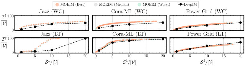
Figure 2. Non-dominated solutions found MOEIM and DeepIM (Ling et al., 2023). For MOEIM, we provide the worst, median and best sets of non-dominated solutions found across $10$ runs. To allow for a direct comparison with the results reported in (Ling et al., 2023), the x-axis and y-axis show, respectively, the seed set size $\mathcal{S}^{\downarrow}$ and the final influence $\mathcal{I}^{\uparrow}$, both normalized w.r.t. the size of each network, $|\mathcal{V}|$. For DeepIM, we show the results available in the original paper, where they are reported separately for each value of $\mathcal{S}^{\downarrow}$/$|\mathcal{V}|$.

Table 3. Results of the statistical tests, performed by using the Holm-Bonferroni procedure (Holm, Sture, 1979), using “MOEIM (all)” as reference (Rank=8.82). Note that, for simplicity of notation, we omit “MOEIM” from the other settings of our algorithm. “Rank” refers to the ranking of the algorithm (the higher, the better). “$z$” is the statistic computed on the rank, “$p$” is the $p$-value, computed as the value of the cumulative normal distribution related to $z$. $\alpha/j$ is the significance threshold adjusted for each row of the table. “Reject” indicates if the sequential null hypothesis (of equivalence between the reference and the algorithm on the row) can be rejected or not.

Method	Rank	$z$	$p$	$\alpha/j$	Rejected
$\mathcal{I}^{\uparrow}$-$\mathcal{S}^{\downarrow}$-$\mathcal{B}^{\downarrow}$	6.56e+00	-4.71e+00	1.21e-06	5.00e-02	True
$\mathcal{I}^{\uparrow}$-$\mathcal{S}^{\downarrow}$-$\mathcal{T}^{\downarrow}$	6.52e+00	-4.83e+00	6.76e-07	2.50e-02	True
$\mathcal{I}^{\uparrow}$-$\mathcal{S}^{\downarrow}$-$\mathcal{F}^{\uparrow}$	4.97e+00	-9.22e+00	1.54e-20	1.67e-02	True
$\mathcal{I}^{\uparrow}$-$\mathcal{S}^{\downarrow}$-$\mathcal{C}^{\uparrow}$	3.55e+00	-1.32e+01	3.24e-40	1.25e-02	True
GGD	3.46e+00	-1.35e+01	9.96e-42	1.00e-02	True
CELF	3.36e+00	-1.38e+01	2.31e-43	8.33e-03	True
MOEA	2.27e+00	-1.69e+01	5.01e-64	7.14e-03	True
$\mathcal{I}^{\uparrow}$-$\mathcal{S}^{\downarrow}$	2.15e+00	-1.72e+01	1.79e-66	6.25e-03	True

6.3. Statistical analysis

To ensure the statistical relevance of our results, we performed a statistical comparison on the hypervolumes achieved by the algorithms under comparison in the first experimental setting [outer color=s1color,fill color=s1color]1, by using the Holm-Bonferroni procedure (Holm, Sture, 1979), with significance threshold $\alpha=0.05$ and the null hypothesis of statistical equivalence. From this test (whose results are shown in Table 3), it emerges that the best-performing method is MOEIM in the “all” setting (i.e., the one considering all six objective functions), which allows rejecting the null hypothesis in all the cases. This is clearly a confirmation of an expected result, as we expect the hypervolume to be maximized when we optimize all the objectives simultaneously.

Table 4. Results of the statistical tests using the Tukey HSD procedure (Tukey, John W, 1949) for pairwise comparisons. Note that, for simplicity of notation, we omit “MOEIM” from the settings of our algorithm. “Mean difference” refers to the mean of the difference on the hypervolume achieved by the methods in each pairwise comparison, “$p\textrm{-adj}$” refers to the adjusted $p$-value, “Lower CI” and “Upper CI” refer to the lower and upper bound for the $95\%$ CI (Confidence Interval). “Reject” indicates if the null hypothesis (of statistical equivalence between Methods 1 and 2) can be rejected or not. We highlight the cases for which the hypothesis can be rejected.

Method 1	Method 2	Mean difference	$p\textrm{-adj}$	Lower CI	Upper CI	Rejected
$\mathcal{I}^{\uparrow}$-$\mathcal{S}^{\downarrow}$	$\mathcal{I}^{\uparrow}$-$\mathcal{S}^{\downarrow}$-$\mathcal{B}^{\downarrow}$	6.90e-3	3.00e-4	2.10e-3	1.16e-2	True
$\mathcal{I}^{\uparrow}$-$\mathcal{S}^{\downarrow}$	$\mathcal{I}^{\uparrow}$-$\mathcal{S}^{\downarrow}$-$\mathcal{C}^{\uparrow}$	1.40e-3	9.93e-1	-3.40e-3	6.20e-3	False
$\mathcal{I}^{\uparrow}$-$\mathcal{S}^{\downarrow}$	$\mathcal{I}^{\uparrow}$-$\mathcal{S}^{\downarrow}$-$\mathcal{F}^{\uparrow}$	2.10e-3	9.06e-1	-2.70e-3	6.90e-3	False
$\mathcal{I}^{\uparrow}$-$\mathcal{S}^{\downarrow}$	$\mathcal{I}^{\uparrow}$-$\mathcal{S}^{\downarrow}$-$\mathcal{T}^{\downarrow}$	7.70e-3	0.00e+0	3.00e-3	1.25e-2	True
$\mathcal{I}^{\uparrow}$-$\mathcal{S}^{\downarrow}$	all	1.20e-2	0.00e+0	7.30e-3	1.68e-2	True
$\mathcal{I}^{\uparrow}$-$\mathcal{S}^{\downarrow}$	CELF	2.40e-3	9.80e-1	-4.60e-3	9.40e-3	False
$\mathcal{I}^{\uparrow}$-$\mathcal{S}^{\downarrow}$	GGD	3.80e-3	2.62e-1	-1.00e-3	8.50e-3	False
$\mathcal{I}^{\uparrow}$-$\mathcal{S}^{\downarrow}$	MOEA	0.00e+0	1.00e+0	-4.70e-3	4.80e-3	False
$\mathcal{I}^{\uparrow}$-$\mathcal{S}^{\downarrow}$-$\mathcal{B}^{\downarrow}$	$\mathcal{I}^{\uparrow}$-$\mathcal{S}^{\downarrow}$-$\mathcal{C}^{\uparrow}$	-5.50e-3	1.09e-2	-1.03e-2	-7.00e-4	True
$\mathcal{I}^{\uparrow}$-$\mathcal{S}^{\downarrow}$-$\mathcal{B}^{\downarrow}$	$\mathcal{I}^{\uparrow}$-$\mathcal{S}^{\downarrow}$-$\mathcal{F}^{\uparrow}$	-4.80e-3	5.11e-2	-9.50e-3	0.00e+0	False
$\mathcal{I}^{\uparrow}$-$\mathcal{S}^{\downarrow}$-$\mathcal{B}^{\downarrow}$	$\mathcal{I}^{\uparrow}$-$\mathcal{S}^{\downarrow}$-$\mathcal{T}^{\downarrow}$	9.00e-4	1.00e+0	-3.90e-3	5.60e-3	False
$\mathcal{I}^{\uparrow}$-$\mathcal{S}^{\downarrow}$-$\mathcal{B}^{\downarrow}$	all	5.20e-3	2.28e-2	4.00e-4	9.90e-3	True
$\mathcal{I}^{\uparrow}$-$\mathcal{S}^{\downarrow}$-$\mathcal{B}^{\downarrow}$	CELF	-4.50e-3	5.53e-1	-1.15e-2	2.50e-3	False
$\mathcal{I}^{\uparrow}$-$\mathcal{S}^{\downarrow}$-$\mathcal{B}^{\downarrow}$	GGD	-3.10e-3	5.19e-1	-7.90e-3	1.60e-3	False
$\mathcal{I}^{\uparrow}$-$\mathcal{S}^{\downarrow}$-$\mathcal{B}^{\downarrow}$	MOEA	-6.90e-3	3.00e-4	-1.16e-2	-2.10e-3	True
$\mathcal{I}^{\uparrow}$-$\mathcal{S}^{\downarrow}$-$\mathcal{C}^{\uparrow}$	$\mathcal{I}^{\uparrow}$-$\mathcal{S}^{\downarrow}$-$\mathcal{F}^{\uparrow}$	7.00e-4	1.00e+0	-4.00e-3	5.50e-3	False
$\mathcal{I}^{\uparrow}$-$\mathcal{S}^{\downarrow}$-$\mathcal{C}^{\uparrow}$	$\mathcal{I}^{\uparrow}$-$\mathcal{S}^{\downarrow}$-$\mathcal{T}^{\downarrow}$	6.40e-3	1.30e-3	1.60e-3	1.11e-2	True
$\mathcal{I}^{\uparrow}$-$\mathcal{S}^{\downarrow}$-$\mathcal{C}^{\uparrow}$	all	1.07e-2	0.00e+0	5.90e-3	1.54e-2	True
$\mathcal{I}^{\uparrow}$-$\mathcal{S}^{\downarrow}$-$\mathcal{C}^{\uparrow}$	CELF	1.00e-3	1.00e+0	-6.00e-3	8.00e-3	False
$\mathcal{I}^{\uparrow}$-$\mathcal{S}^{\downarrow}$-$\mathcal{C}^{\uparrow}$	GGD	2.40e-3	8.36e-1	-2.40e-3	7.10e-3	False
$\mathcal{I}^{\uparrow}$-$\mathcal{S}^{\downarrow}$-$\mathcal{C}^{\uparrow}$	MOEA	-1.40e-3	9.94e-1	-6.10e-3	3.40e-3	False
$\mathcal{I}^{\uparrow}$-$\mathcal{S}^{\downarrow}$-$\mathcal{F}^{\uparrow}$	$\mathcal{I}^{\uparrow}$-$\mathcal{S}^{\downarrow}$-$\mathcal{T}^{\downarrow}$	5.60e-3	8.10e-3	8.00e-4	1.04e-2	True
$\mathcal{I}^{\uparrow}$-$\mathcal{S}^{\downarrow}$-$\mathcal{F}^{\uparrow}$	all	9.90e-3	0.00e+0	5.10e-3	1.47e-2	True
$\mathcal{I}^{\uparrow}$-$\mathcal{S}^{\downarrow}$-$\mathcal{F}^{\uparrow}$	CELF	3.00e-4	1.00e+0	-6.80e-3	7.30e-3	False
$\mathcal{I}^{\uparrow}$-$\mathcal{S}^{\downarrow}$-$\mathcal{F}^{\uparrow}$	GGD	1.60e-3	9.79e-1	-3.10e-3	6.40e-3	False
$\mathcal{I}^{\uparrow}$-$\mathcal{S}^{\downarrow}$-$\mathcal{F}^{\uparrow}$	MOEA	-2.10e-3	9.12e-1	-6.90e-3	2.70e-3	False
$\mathcal{I}^{\uparrow}$-$\mathcal{S}^{\downarrow}$-$\mathcal{T}^{\downarrow}$	all	4.30e-3	1.17e-1	-5.00e-4	9.10e-3	False
$\mathcal{I}^{\uparrow}$-$\mathcal{S}^{\downarrow}$-$\mathcal{T}^{\downarrow}$	CELF	-5.40e-3	3.03e-1	-1.24e-2	1.70e-3	False
$\mathcal{I}^{\uparrow}$-$\mathcal{S}^{\downarrow}$-$\mathcal{T}^{\downarrow}$	GGD	-4.00e-3	1.89e-1	-8.80e-3	8.00e-4	False
$\mathcal{I}^{\uparrow}$-$\mathcal{S}^{\downarrow}$-$\mathcal{T}^{\downarrow}$	MOEA	-7.70e-3	0.00e+0	-1.25e-2	-2.90e-3	True
all	CELF	-9.70e-3	7.00e-4	-1.67e-2	-2.60e-3	True
all	GGD	-8.30e-3	0.00e+0	-1.31e-2	-3.50e-3	True
all	MOEA	-1.20e-2	0.00e+0	-1.68e-2	-7.20e-3	True
CELF	GGD	1.40e-3	1.00e+0	-5.70e-3	8.40e-3	False
CELF	MOEA	-2.40e-3	9.81e-1	-9.40e-3	4.70e-3	False
GGD	MOEA	-3.70e-3	2.71e-1	-8.50e-3	1.00e-3	False

Moreover, to statistically assess the pairwise comparisons among the algorithms, we also performed a Tukey HSD test (Tukey, John W, 1949) for multiple comparisons, keeping the same significance threshold and null hypothesis. These results (presented in Table 4) show that, while in Table 2 all the MOEIM settings seem to outperform the baseline methods, only the “all” setting reliably does so. It is worth noting that this may result be due to the fact that, since this test is based on the actual Hypervolumes (instead of their ranking, as in the Holm-Bonferroni test) and we are aggregating the results obtained across several datasets, the standard deviation of the Hypervolumes obtained with the other MOEIM settings proposed in this paper is too high to lead to statistically significant results.

Finally, it is important to note that we could not perform any statistical test between our methods and DeepIM considered in the second experimental setting [outer color=s2color,fill color=s2color]2, since the DeepIM results have been taken directly from the original paper without raw data availability.

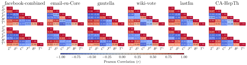
Figure 3. Pearson correlation among the objectives ($\mathcal{I}^{\uparrow}$: Influence; $\mathcal{S}^{\downarrow}$: Seed set size; $\mathcal{C}^{\uparrow}$: Communities; $\mathcal{F}^{\uparrow}$: Fairness; $\mathcal{B}^{\downarrow}$: Budget; $\mathcal{T}^{\downarrow}$: Time). This correlation has been computed over the results of the 10 runs available for the “MOEIM (all)” setting (see Table 2 for details). Top row: IC model, bottom row: WC model.

6.4. Analysis of objective function correlation

We conclude our analysis studying the correlation between the objective functions. This study has been conducted to better understand the hypervolume trend on $\mathcal{T}^{\downarrow}$ of Table 2 and explain the reason why the hypervolume computed over ($\mathcal{I}^{\uparrow}$-$\mathcal{S}^{\downarrow}$) decreases when adding objective functions. Figure 3 displays the Pearson correlation among the proposed objective functions. Such correlation has been computed separately for each $\langle$dataset, propagation model$\rangle$ combination on the results of MOEIM (all). For this analysis, each entry corresponds to the vector of the normalized objectives (see Section 6.1) for each non-dominated solution found across the $10$ runs of MOEIM (all). The analysis clearly shows how all the objective functions added to the base setting objectives (i.e., $\mathcal{I}^{\uparrow}$ and $\mathcal{S}^{\downarrow}$) are negatively correlated with them. In fact, $\mathcal{C}^{\uparrow}$ and $\mathcal{F}^{\uparrow}$ are negatively correlated (w.r.t. to both $\mathcal{I}^{\uparrow}$ and $\mathcal{S}^{\downarrow}$), while $\mathcal{B}^{\downarrow}$ and $\mathcal{T}^{\downarrow}$ are positively correlated (always w.r.t. $\mathcal{I}^{\uparrow}$ and $\mathcal{S}^{\downarrow}$), but these latter two objectives are minimized. The highest correlation turns out to be between $\mathcal{B}^{\downarrow}$ and $\mathcal{I}^{\uparrow}$, since as expected selecting (in the seed set) nodes with high out-degree leads to improving the overall influence spread, and between $\mathcal{S}^{\downarrow}$ and $\mathcal{I}^{\uparrow}$. Of note, the correlation between $\mathcal{C}^{\uparrow}$ and $\mathcal{F}^{\uparrow}$ turns out to be extremely high, since such objectives, even tough formulated differently, share the same spirit of fair allocation on either the final influence or the seed set allocation. To conclude, the reason why, in some cases, the hypervolume in the $\mathcal{B}^{\downarrow}$ or “all” settings is higher w.r.t. ($\mathcal{I}^{\uparrow}$-$\mathcal{S}^{\downarrow}$-$\mathcal{T}^{\downarrow}$) is due to the positive correlation between $\mathcal{T}^{\downarrow}$ with both $\mathcal{B}^{\downarrow}$ and $\mathcal{S}^{\downarrow}$.

7. Conclusions

We presented a new setting for the IM problem, where up to six objective functions are considered in the optimization process. For solving such a task, we proposed MOEIM, a MOEA designed to leverage graph information thanks to the use of graph-aware operators and a smart initialization of the initial population. The numerical results confirm the effectiveness of the proposed approach w.r.t. the state of the art, including a recently proposed DL-based method. Moreover, our results allowed us to investigate the correlation objectives, providing insightful information on IM.

The approach presented in this work opens up several possibilities to expand the IM problem even further, as new objectives can be easily added to our codebase. Moreover, while in this work we mainly focused on static graphs and propagation models taken independently, another possibility for future works could be to conduct similar multi-objective studies on dynamic graphs, or to aim at assessing the solutions robustness w.r.t. multiple propagation models.

References

• (1)
• Ali et al. (2023) Junaid Ali, Mahmoudreza Babaei, Abhijnan Chakraborty, Baharan Mirzasoleiman, Krishna Gummadi, and Adish Singla. 2023. On the fairness of time-critical influence maximization in social networks. IEEE Transactions on Knowledge and Data Engineering 35, 3 (2023), 2875–2886.
• Becker et al. (2022) Ruben Becker, Gianlorenzo D’angelo, Sajjad Ghobadi, and Hugo Gilbert. 2022. Fairness in influence maximization through randomization. Journal of Artificial Intelligence Research 73 (2022), 1251–1283.
• Benedek Rozemberczki and Rik Sarkar (2020) Benedek Rozemberczki and Rik Sarkar. 2020. Characteristic Functions on Graphs: Birds of a Feather, from Statistical Descriptors to Parametric Models. In International Conference on Information and Knowledge Management. ACM, New York, NY, USA, 1325–1334.
• Bian, Song and Guo, Qintian and Wang, Sibo and Yu, Jeffrey Xu (2020) Bian, Song and Guo, Qintian and Wang, Sibo and Yu, Jeffrey Xu. 2020. Efficient algorithms for budgeted influence maximization on massive social networks. Proceedings of the VLDB Endowment 13, 9 (2020), 1498–1510.
• Biswas et al. (2022a) Tarun K Biswas, Alireza Abbasi, and Ripon K Chakrabortty. 2022a. An improved clustering based multi-objective evolutionary algorithm for influence maximization under variable-length solutions. Knowledge-Based Systems 256 (2022), 109856.
• Biswas et al. (2022b) Tarun K Biswas, Alireza Abbasi, and Ripon K Chakrabortty. 2022b. Multi-Objective Influence Maximization Under Varying-Size Solutions and Constraints. In IEEE/ACM International Conference on Advances in Social Networks Analysis and Mining. IEEE, New York, NY, USA, 285–292.
• Bucur and Iacca (2016) Doina Bucur and Giovanni Iacca. 2016. Influence maximization in social networks with genetic algorithms. In Applications of Evolutionary Computation. Springer, Cham, Switzerland, 379–392.
• Bucur et al. (2017) Doina Bucur, Giovanni Iacca, Andrea Marcelli, Giovanni Squillero, and Alberto Tonda. 2017. Multi-objective evolutionary algorithms for influence maximization in social networks. In Applications of Evolutionary Computation. Springer, Cham, Switzerland, 221–233.
• Bucur et al. (2018) Doina Bucur, Giovanni Iacca, Andrea Marcelli, Giovanni Squillero, and Alberto Tonda. 2018. Improving multi-objective evolutionary influence maximization in social networks. In Applications of Evolutionary Computation. Springer, Cham, Switzerland, 117–124.
• Chawla, Aviral and Cheney, Nick (2023) Chawla, Aviral and Cheney, Nick. 2023. Neighbor-Hop Mutation for Genetic Algorithm in Influence Maximization. In Conference on Genetic and Evolutionary Computation Companion. ACM, New York, NY, USA, 187–190.
• Chen et al. (2023) Tiantian Chen, Siwen Yan, Jianxiong Guo, and Weili Wu. 2023. ToupleGDD: A Fine-Designed Solution of Influence Maximization by Deep Reinforcement Learning. IEEE Transactions on Computational Social Systems (early access) (2023), 1–12.
• Chen et al. (2012) Wei Chen, Wei Lu, and Ning Zhang. 2012. Time-critical influence maximization in social networks with time-delayed diffusion process. In AAAI Conference on Artificial Intelligence, Vol. 26. Association for the Advancement of Artificial Intelligence, Washington DC, USA, 591–598.
• Chen, Wei and Wang, Yajun and Yang, Siyu (2009) Chen, Wei and Wang, Yajun and Yang, Siyu. 2009. Efficient influence maximization in social networks. In ACM SIGKDD International Conference on Knowledge Discovery and Data Mining. ACM, New York, NY, USA, 199–208.
• Cunegatti et al. (2022) Elia Cunegatti, Giovanni Iacca, and Doina Bucur. 2022. Large-scale multi-objective influence maximisation with network downscaling. In Parallel Problem Solving from Nature. Springer, Cham, Switzerland, 207–220.
• Deb, K. and Pratap, A. and Agarwal, S. and Meyarivan, T. (2002) Deb, K. and Pratap, A. and Agarwal, S. and Meyarivan, T. 2002. A fast and elitist multiobjective genetic algorithm: NSGA-II. IEEE Transactions on Evolutionary Computation 6, 2 (2002), 182–197.
• Farnad et al. (2020) Golnoosh Farnad, Behrouz Babaki, and Michel Gendreau. 2020. A unifying framework for fairness-aware influence maximization. In The Web Conference Companion. ACM, New York, NY, USA, 714–722.
• Feng et al. (2023) Yuting Feng, Ankitkumar Patel, Bogdan Cautis, and Hossein Vahabi. 2023. Influence Maximization with Fairness at Scale. arXiv preprint arXiv:2306.01587.
• Giovanni Iacca and Kateryna Konotopska and Doina Bucur and Alberto Tonda (2021) Giovanni Iacca and Kateryna Konotopska and Doina Bucur and Alberto Tonda. 2021. An evolutionary framework for maximizing influence propagation in social networks. Software Impacts 9 (2021), 100107.
• Gleiser, Pablo M and Danon, Leon (2003) Gleiser, Pablo M and Danon, Leon. 2003. Community structure in jazz. Advances in complex systems 6, 04 (2003), 565–573.
• Gong and Guo (2023) Hao Gong and Chunxiang Guo. 2023. Influence maximization considering fairness: A multi-objective optimization approach with prior knowledge. Expert Systems with Applications 214 (2023), 119138.
• Gong, Maoguo and Yan, Jianan and Shen, Bo and Ma, Lijia and Cai, Qing (2016) Gong, Maoguo and Yan, Jianan and Shen, Bo and Ma, Lijia and Cai, Qing. 2016. Influence maximization in social networks based on discrete particle swarm optimization. Information Sciences 367 (2016), 600–614.
• Goyal et al. (2011) Amit Goyal, Wei Lu, and Laks VS Lakshmanan. 2011. CELF++ optimizing the greedy algorithm for influence maximization in social networks. In International Conference on World Wide Web Companion. ACM, New York, NY, USA, 47–48.
• Holm, Sture (1979) Holm, Sture. 1979. A simple sequentially rejective multiple test procedure. Scandinavian journal of statistics 6, 2 (1979), 65–70.
• Jiang, Qingye and Song, Guojie and Gao, Cong and Wang, Yu and Si, Wenjun and Xie, Kunqing (2011) Jiang, Qingye and Song, Guojie and Gao, Cong and Wang, Yu and Si, Wenjun and Xie, Kunqing. 2011. Simulated annealing based influence maximization in social networks. In AAAI Conference on Artificial intelligence, Vol. 25. Association for the Advancement of Artificial Intelligence, Washington DC, USA, 127–132.
• Jure Leskovec and Andrej Krevl (2014) Jure Leskovec and Andrej Krevl. 2014. SNAP Datasets: Stanford Large Network Dataset Collection. http://snap.stanford.edu/data.
• Kempe et al. (2003) David Kempe, Jon Kleinberg, and Éva Tardos. 2003. Maximizing the spread of influence through a social network. In ACM SIGKDD International Conference on Knowledge Discovery and Data Mining. ACM, New York, NY, USA, 137–146.
• Khajehnejad et al. (2020) Moein Khajehnejad, Ahmad Asgharian Rezaei, Mahmoudreza Babaei, Jessica Hoffmann, Mahdi Jalili, and Adrian Weller. 2020. Adversarial graph embeddings for fair influence maximization over social networks. arXiv preprint arXiv:2005.04074.
• Konotopska, Kateryna and Iacca, Giovanni (2021) Konotopska, Kateryna and Iacca, Giovanni. 2021. Graph-aware evolutionary algorithms for influence maximization. In Genetic and Evolutionary Computation Conference Companion. ACM, New York, NY, USA, 1467–1475.
• Lee, Jong-Ryul and Chung, Chin-Wan (2014) Lee, Jong-Ryul and Chung, Chin-Wan. 2014. A fast approximation for influence maximization in large social networks. In International Conference on World Wide Web. ACM, New York, NY, USA, 1157–1162.
• Leskovec et al. (2007) Jure Leskovec, Andreas Krause, Carlos Guestrin, Christos Faloutsos, Jeanne VanBriesen, and Natalie Glance. 2007. Cost-effective outbreak detection in networks. In ACM SIGKDD International Conference on Knowledge Discovery and Data Mining. ACM, New York, NY, USA, 420–429.
• Leskovec, Jure and Huttenlocher, Daniel and Kleinberg, Jon (2010) Leskovec, Jure and Huttenlocher, Daniel and Kleinberg, Jon. 2010. Signed networks in social media. In SIGCHI Conference on Human Factors in Computing Systems. ACM, New York, NY, USA, 1361–1370.
• Leskovec, Jure and Kleinberg, Jon and Faloutsos, Christos (2007) Leskovec, Jure and Kleinberg, Jon and Faloutsos, Christos. 2007. Graph evolution: Densification and shrinking diameters. ACM Transactions on Knowledge Discovery from Data 1, 1 (2007), 2–es.
• Leskovec, Jure and Mcauley, Julian (2012) Leskovec, Jure and Mcauley, Julian. 2012. Learning to discover social circles in ego networks. Advances in Neural Information Processing Systems 25 (2012), 9 pages.
• Li et al. (2023) Hui Li, Mengting Xu, Sourav S Bhowmick, Joty Shafiq Rayhan, Changsheng Sun, and Jiangtao Cui. 2023. PIANO: Influence maximization meets deep reinforcement learning. IEEE Transactions on Computational Social Systems 10, 3 (2023), 1288–1300.
• Ling et al. (2023) Chen Ling, Junji Jiang, Junxiang Wang, My T Thai, Renhao Xue, James Song, Meikang Qiu, and Liang Zhao. 2023. Deep graph representation learning and optimization for influence maximization. In International Conference on Machine Learning. PMLR, Honolulu, HI, USA, 21350–21361.
• Liu et al. (2012) Bo Liu, Gao Cong, Dong Xu, and Yifeng Zeng. 2012. Time constrained influence maximization in social networks. In IEEE International Conference on Data Mining. IEEE, New York, NY, USA, 439–448.
• Lotf, Jalil Jabari and Azgomi, Mohammad Abdollahi and Dishabi, Mohammad Reza Ebrahimi (2022) Lotf, Jalil Jabari and Azgomi, Mohammad Abdollahi and Dishabi, Mohammad Reza Ebrahimi. 2022. An improved influence maximization method for social networks based on genetic algorithm. Physica A: Statistical Mechanics and its Applications 586 (2022), 126480.
• Ma, Lijia and Shao, Zengyang and Li, Xiaocong and Lin, Qiuzhen and Li, Jianqiang and Leung, Victor CM and Nandi, Asoke K (2022) Ma, Lijia and Shao, Zengyang and Li, Xiaocong and Lin, Qiuzhen and Li, Jianqiang and Leung, Victor CM and Nandi, Asoke K. 2022. Influence maximization in complex networks by using evolutionary deep reinforcement learning. IEEE Transactions on Emerging Topics in Computational Intelligence 7 (2022), 995–1009. Issue 4.
• McCallum et al. (2000) Andrew Kachites McCallum, Kamal Nigam, Jason Rennie, and Kristie Seymore. 2000. Automating the construction of internet portals with machine learning. Information Retrieval 3 (2000), 127–163.
• Olivares et al. (2021) Rodrigo Olivares, Francisco Muñoz, and Fabián Riquelme. 2021. A multi-objective linear threshold influence spread model solved by swarm intelligence-based methods. Knowledge-Based Systems 212 (2021), 106623.
• Panagopoulos et al. (2020) George Panagopoulos, Fragkiskos D Malliaros, and Michalis Vazirgiannis. 2020. Multi-task learning for influence estimation and maximization. IEEE Transactions on Knowledge and Data Engineering 34, 9 (2020), 4398–4409.
• Peixoto, Tiago P (2020) Peixoto, Tiago P. 2020. The Netzschleuder network catalogue and repository. https://networks.skewed.de.
• Perrault, Pierre and Healey, Jennifer and Wen, Zheng and Valko, Michal (2020) Perrault, Pierre and Healey, Jennifer and Wen, Zheng and Valko, Michal. 2020. Budgeted online influence maximization. In International Conference on Machine Learning. PMLR, virtual event, 7620–7631.
• Pham et al. (2019) Canh V Pham, Hieu V Duong, Huan X Hoang, and My T Thai. 2019. Competitive influence maximization within time and budget constraints in online social networks: An algorithmic approach. Applied Sciences 9, 11 (2019), 2274.
• Razaghi et al. (2022) Behnam Razaghi, Mehdy Roayaei, and Nasrollah Moghadam Charkari. 2022. On the Group-Fairness-Aware Influence Maximization in Social Networks. IEEE Transactions on Computational Social Systems 10, 6 (2022), 3406–3414.
• Riquelme et al. (2023) Fabián Riquelme, Francisco Muñoz, and Rodrigo Olivares. 2023. A depth-based heuristic to solve the multi-objective influence spread problem using particle swarm optimization. OPSEARCH 60 (2023), 1267–1285.
• Rossi and Ahmed (2015) Ryan Rossi and Nesreen Ahmed. 2015. The network data repository with interactive graph analytics and visualization. In AAAI Conference on Artificial Intelligence, Vol. 29. Association for the Advancement of Artificial Intelligence, Washington DC, USA, 4292–4293.
• Rui et al. (2023) Xiaobin Rui, Zhixiao Wang, Jiayu Zhao, Lichao Sun, and Wei Chen. 2023. Scalable Fair Influence Maximization. Advances in Neural Information Processing Systems 1 (2023), 12 pages.
• Shang, Ke and Ishibuchi, Hisao and He, Linjun and Pang, Lie Meng (2020) Shang, Ke and Ishibuchi, Hisao and He, Linjun and Pang, Lie Meng. 2020. A survey on the hypervolume indicator in evolutionary multiobjective optimization. IEEE Transactions on Evolutionary Computation 25, 1 (2020), 1–20.
• Stoica et al. (2020) Ana-Andreea Stoica, Jessy Xinyi Han, and Augustin Chaintreau. 2020. Seeding network influence in biased networks and the benefits of diversity. In The Web Conference. ACM, New York, NY, USA, 2089–2098.
• Tang et al. (2018) Jing Tang, Xueyan Tang, Xiaokui Xiao, and Junsong Yuan. 2018. Online processing algorithms for influence maximization. In ACM SIGMOD International Conference on Management of Data. ACM, New York, NY, USA, 991–1005.
• Tang et al. (2015) Youze Tang, Yanchen Shi, and Xiaokui Xiao. 2015. Influence maximization in near-linear time: A martingale approach. In ACM SIGMOD International Conference on Management of Data. ACM, New York, NY, USA, 1539–1554.
• Tong et al. (2020) Guangmo Tong, Ruiqi Wang, Zheng Dong, and Xiang Li. 2020. Time-constrained adaptive influence maximization. IEEE Transactions on Computational Social Systems 8, 1 (2020), 33–44.
• Traag, Vincent A and Waltman, Ludo and Van Eck, Nees Jan (2019) Traag, Vincent A and Waltman, Ludo and Van Eck, Nees Jan. 2019. From Louvain to Leiden: guaranteeing well-connected communities. Scientific reports 9, 1 (2019), 5233.
• Tsang et al. (2019) Alan Tsang, Bryan Wilder, Eric Rice, Milind Tambe, and Yair Zick. 2019. Group-fairness in influence maximization. arXiv preprint arXiv:1903.00967.
• Tukey, John W (1949) Tukey, John W. 1949. Comparing individual means in the analysis of variance. Biometrics 5, 2 (1949), 99–114.
• Wang et al. (2016) Xiaojie Wang, Xue Zhang, Chengli Zhao, and Dongyun Yi. 2016. Maximizing the spread of influence via generalized degree discount. PloS ONE 11, 10 (2016), e0164393.
• Watts, Duncan J and Strogatz, Steven H (1998) Watts, Duncan J and Strogatz, Steven H. 1998. Collective dynamics of ‘small-world’networks. Nature 393, 6684 (1998), 440–442.