Robust Numerical Algebraic Geometry

Abstract

The field of numerical algebraic geometry consists of algorithms for numerically solving systems of polynomial equations. When the system is exact, such as having rational coefficients, the solution set is well-defined. However, for a member of a parameterized family of polynomial systems where the parameter values may be measured with imprecision or arise from prior numerical computations, uncertainty may arise in the structure of the solution set, including the number of isolated solutions, the existence of higher dimensional solution components, and the number of irreducible components along with their multiplicities. The loci where these structures change form a stratification of exceptional algebraic sets in the space of parameters. We describe methodologies for making the interpretation of numerical results more robust by searching for nearby parameter values on an exceptional set. We demonstrate these techniques on several illustrative examples and then treat several more substantial problems arising from the kinematics of mechanisms and robots.

1 Introduction

Numerical algebraic geometry concerns algorithms for numerically solving systems of polynomial equations, primarily based on homotopy methods, often also referred to as polynomial continuation. Reference texts for numerical algebraic geometry are [6, 44], and software packages that implement its algorithms are available in [5, 9, 27, 48]. Built on a foundation of methods for finding all isolated solutions, the field has grown to include algorithms for computing the irreducible decomposition of algebraic sets along with operations such as membership testing, intersection, and projection. The basic construct of the field is a witness set, say ${\mathcal{W}}$, in which a pure $D$-dimensional algebraic set, say $X\subset{\mathbb{C}}^{n}$, is represented by a structure having three members:

$${\mathcal{W}}=\{f,L,W\}$$ (1)

where $f:{\mathbb{C}}^{n}\rightarrow{\mathbb{C}}^{k}$ is a polynomial system such that $X$ is a $D$-dimensional component of $V(f)=\{x\in{\mathbb{C}}^{n}\,|\,f(x)=0\}$, $L:{\mathbb{C}}^{n}\rightarrow{\mathbb{C}}^{D}$ is a slicing system of $D$ generic linear polynomials, and $W=X\cap V(L)$ is a witness point set for $X$. Given a witness set, one can sample the set it represents by moving its slicing system in a homotopy. Given witness sets for two components, one can compute their intersection, obtaining witness sets for the components of the intersection [23]. A witness set can be decomposed into its irreducible components using monodromy [41] to group together points on the same irreducible component and using a trace test [8, 10, 17, 28, 42] to verify when this process is complete. Algorithms built on these and related techniques compute a numerical irreducible decomposition of $V(f)$, producing a collection of witness sets, one for each irreducible component. In a similar fashion, one may construct pseudo-witness sets for projections of algebraic sets [19, 20], which is the geometric equivalent of symbolic elimination. Altogether, using algorithms for intersection, union, projection, and membership testing, one can represent and manipulate constructible algebraic sets.

Applications of algebraic geometry often involve parameterized families of polynomial systems of the form $f(x;p):{\mathbb{C}}^{n}\times{\mathbb{C}}^{m}\rightarrow{\mathbb{C}}^{k}$, where $x$ is an array of variables and $p$ is an array of parameters. For example, in kinematic analysis, $x$ may be variables describing the relative displacement at joints between parts while $p$ may describe the length of links or the axis of a rotational joint. In kinematic synthesis, where one seeks to find a mechanism to produce a desired motion, these roles may be interchanged. The long history of research in kinematics and its applications to mechanisms and robotics is extensive; [38, 52] provide useful overviews. In multi-view computer vision, the variables of a scene reconstruction describe the location of objects and cameras in three-dimensional space while the parameters are the coordinates of features observed in the camera images [1, 13, 24, 30]. In chemical equilibrium, concentrations are variables and reaction rates are parameters [34, Chap. 9] and [12, 37]. In short, in a single instance of the family, variables are the unknowns while parameters are given, and the parameter space defines a family of problems having the same polynomial structure. In the simplest case, the parameters are merely the coefficients of polynomials with a fixed set of monomials while, in many applications, the coefficients are often polynomial functions of the parameters. In general, one can consider a parameter space that is an irreducible algebraic set or, with minor additional conditions, even a complex analytic set [36]. However, for simplicity, we will assume here that the parameter space is the complex Euclidean space ${\mathbb{C}}^{m}$.

The algorithms of numerical algebraic geometry compute using floating point arithmetic, so function evaluations and solution points are consequently inexact. Furthermore, in applications, parameters may be values measured with imprecision or they may be numerical values produced in prior stages of computation. In light of these uncertainties, the results reported by the algorithms may require interpretation. For example, a coordinate of a solution point computed as near zero may indicate that there is an exact solution nearby with that coordinate exactly zero, but this is not assured. Moreover, if the polynomial system is given with uncertain parameters or with coefficients presented as floating point values, there is some uncertainty about which problem is being posed. The interpretation of the solution set, such as classifying how many endpoints of a homotopy have converged to finite solution points versus how many have diverged to infinity, is subject to judgements about round-off errors from inexactly evaluating inexactly specified polynomials. Similar judgements must be made when categorizing singular versus nonsingular solutions, sorting solutions versus nonsolutions when utilizing randomization, concluding that a witness set is complete via a trace test, or counting multiplicities according to how many homotopy paths converge to (nearly) the same point. Our aim in this article is to lay out methodologies for making these interpretations more robust yielding robust numerical algebraic geometry.

In a parameterized family, the irreducible decomposition has the same structure for generic parameters, that is, the sets of parameters where the structure changes lie on proper algebraic subsets of the parameter space. By structure, we mean features over the complex numbers described by integers, such as the number of irreducible components, their dimensions and degrees, and the multiplicity of the witness points. Within any irreducible algebraic subset of parameter space, there may exist algebraic subsets of lower dimension where these integer features change again, creating a stratification of algebraic sets of successively greater specialization. In an early discussion of this phenomenon, Kahan [26] called such sets pejorative manifolds, but we prefer the more neutral term exceptional sets. Typically, an analyst would like to know that the problem they have posed is close to an exceptional set. Moreover, since such sets have zero measure in their containing parameter space, the fact that a posed problem falls quite close to an exceptional set may indicate that this is not a coincidence, and in fact, the exceptional case is the true item of interest. Moreover, constraining the problem to lie on an exceptional set can convert an ill-conditioned problem into a well-conditioned one [26].

Factoring a single multivariate polynomial presents a special case of the phenomena we presently address. Wu and Zeng [53] note that factorization of such a polynomial is ill-posed when coefficient perturbations are considered since the factors change discontinuously as the coefficients approach a factorization submanifold. Their answer to this problem is to define a metric for the distance between polynomials and a partial ordering on the factorization structures. This partial ordering corresponds to algebraic set inclusion in the stratification of factorization structures, and in the parlance of Wu and Zeng, each such set is said to be more singular than any set that contains it. (Roughly, a polynomial with more factors is more singular than one with fewer, and for the same degree, a factor appearing with multiplicity is more singular that a product of distinct factors.) Wu and Zeng regularize the numerical factorization problem by requiring the user to provide an uncertainty ball around the given polynomial. Among all the possible factorization manifolds that intersect the uncertainty ball, they define the numerical factorization to be the nearest polynomial on the exceptional set of highest singularity. As the radius of the uncertainty ball grows, the numerical factorization may change to one of higher singularity. So, while the problem remains ill-posed at critical radii, it has become well-posed everywhere else. In the case of a single polynomial of moderate degree, the number of possible specializations is small enough that one can enumerate them all. This gives the potential of finding the unique numerical factorization for most uncertainty radii, and a finite list of alternatives for any range of radii, functionalities provided by Wu and Zeng’s software package.

For parameterized systems of polynomials, enumeration of the possible irreducible decomposition structures is a formidable task, and we do not attempt it here. However, in the process of computing a decomposition, there typically will be only a few places where the uncertainty in judging how to classify points warrants exploration of the alternatives. The same can be said for more limited objectives, such as computing only the isolated solutions of a system by homotopy, where one may question the number of solution paths deemed to have landed at infinity or observe a cluster of path endpoints that might indicate a single solution point of higher multiplicity. If the uncertainty is due solely to floating point round-off and we have access to either a symbolic description or a refinable numerical description of the parameter values, then the correct judgement can be made with high confidence by increasing the precision of the computation. Such results might then be certified either by symbolic computations or by verifiable numerics, such as Smale’s alpha theory [39] (see also [7, Ch. 8]) or by techniques from interval analysis [32]. Our concern in this article is for cases where there is inherent uncertainty in the parameters. This may arise from empirical measurements of the parameters or, perhaps, the parameters arise from prior computations in finite precision. We assume that the questionable structural element has been identified and our task is to find the nearest point in parameter space where the special structure occurs.

After describing some robustness scenarios in Section 2, Section 3 provides a framework for robustness in numerical algebraic geometry. This framework is then applied to a variety of structures: fewer finite solutions in Section 4, existence of higher-dimensional components in Section 5, components that further decompose into irreducible components in Section 6, and solution sets of higher multiplicity in Section 7. We formulate the algebraic conditions implied by each type of structure and use local optimization techniques to find a nearby set of parameters satisfying them. After treating each type of specialized structure and illustrating on a small example, we show the effectiveness of the approach on three more substantial problems coming from the kinematics of mechanisms and robots in Section 8. A short conclusion is provided in Section 9. Files for the examples, which are all computed using Bertini [5], are available at https://doi.org/10.7274/25328878.

2 Robustness scenarios

Before presenting our approach to robustifying numerical algebraic geometry, we discuss scenarios where proximity to an exceptional set leads to ill-conditioning.

To abbreviate the discussion, we use the phrase “with probability one” as shorthand for the more precise, and stronger, condition that exceptions are a proper algebraic subset of the relevant parameter space, where the parameter space in question should be clear from context. Similarly, a point in parameter space is “generic” if it lies in the dense Zariski-open set that is the complement of the set of exceptions. For example, the reference to “a system of $D$ generic linear polynomials,” $L:{\mathbb{C}}^{n}\rightarrow{\mathbb{C}}^{D}$, just after (1) means a system of the form $Ax+b$ where matrix $[A\>\>b\,]$ has been chosen from the dense Zariski-open subset of ${\mathbb{C}}^{D\times(n+1)}$ where $V(L)$ intersects $X$ transversely. In numerical work, we make the assumption that a random number generator suffices for choosing generic points.

Our discussion utilizes the concept of a fiber product [45]. For algebraic sets $A$ and $B$ with algebraic maps $\pi_{A}:A\rightarrow Y$ and $\pi_{B}:B\rightarrow Y$, the fiber product of $A$ with $B$ over $Y$ is

$$A\times_{Y}B=\{(a,b)\in A\times B\,|\,\pi_{A}(a)=\pi_{B}(b)\}.$$ (2)

One may similarly form fiber products between three or more algebraic sets. In this article, the maps involved in forming fiber products will all be natural projections of the form $(x,p)\mapsto p$. Moreover, for polynomial systems $f,g:{\mathbb{C}}^{n}\times{\mathbb{C}}^{m}\rightarrow{\mathbb{C}}^{k}$, if $A$ and $B$ in ${\mathbb{C}}^{n}\times{\mathbb{C}}^{m}$ are irreducible components of $V(f(x,p))$ and $V(g(x,p))$, respectively, then the fiber product of $A$ with $B$ over ${\mathbb{C}}^{m}$ is an algebraic set in $V(f(x_{1},p_{1}),g(x_{2},p_{2}),p_{1}-p_{2})$, a so-called reduction to the diagonal which is isomorphic to an algebraic set in $V(f(x_{1},p),g(x_{2},p))\subset{\mathbb{C}}^{n}\times{\mathbb{C}}^{n}\times{\mathbb{C}}^{m}$. In this situation, we refer to $\{f(x_{1},p),g(x_{2},p)\}$ as a fiber product system. We note the convention used throughout is that $f(x,p)$ means that both $x$ and $p$ are considered as variables which is in contrast to $f(x;p)$ where $x$ are variables and $p$ are parameters.

2.1 Multiplicity example

As a simple first example, consider solving $V(f)$ for the single polynomial $f=x^{2}+2\sqrt{2}x+2$, which has the factorization $(x+\sqrt{2})^{2}$ and hence $V(f)$ is the single point $x=-\sqrt{2}$ of multiplicity 2. If instead of the exact symbolic form of $f$, we are given an eight-digit version of it, say

$${\tilde{f}}_{8}=x^{2}+2.8284271x+2,$$

the Matlab roots command, operating in double precision, returns the two roots

$$x_{8}=-1.414213550000000\pm 0.000187073241389\text{i}$$

where $\text{i}=\sqrt{-1}$. Using these roots as initial guesses for Newton’s method, the solutions of the sixteen-digit version of $f$,

$${\tilde{f}}_{16}=x^{2}+2.828427124746190x+2,$$

are computed in double precision as

$$x_{16}=-1.414213553589213\pm 0.000000183520060\text{i}.$$

One may work the problem in increasingly higher precision by considering a sequence of approximations $a_{\ell}$ of $2\sqrt{2}$ rounded off to $\ell$ digits. For every $\ell$, ${\tilde{f}}_{\ell}=x^{2}+a_{\ell}x+2$ has a pair of roots in the vicinity of $-\sqrt{2}$. A numerical package with adjustable precision can refine ${\tilde{f}}_{\ell}$ and a solution $x_{\ell}$ until $|x_{\ell}+\sqrt{2}|$ is smaller than any positive error tolerance one might set. Whether a computer program using this refinement process reports two isolated roots or one double root depends on settings for its precision and tolerance. If the same program is only given ${\tilde{f}}_{8}$ or ${\tilde{f}}_{16}$, the roots stay distinct no matter what precision is used for Newton’s method.

We can stabilize this situation by asking if there exists a nearby polynomial with a double root. That is, we ask if there is a polynomial near to ${\tilde{f}}_{8}$ of the form $\hat{f}(x;p)=x^{2}+px+2$ with a root that also satisfies the derivative $\hat{f}^{\prime}(x;p)=2x+p$. Solving $V(\hat{f}(x,p),\hat{f}^{\prime}(x,p))$ in ${\mathbb{C}}^{2}$ with Newton’s method and an initial guess taking $x=x_{8}$ and $p=a_{8}$, returns

$$(\hat{x},\hat{p})=(-1.414213562373095,2.828427124746190),$$

where the imaginary parts have converged to zero within machine epsilon. Moreover, the Jacobian matrix for this structured system is clearly nonsingular:

$$J\left[\begin{array}[]{c}\hat{f}\\ \hat{f}^{\prime}\end{array}\right]=\left[\begin{array}[]{cc}2x+p&x\\ 2&1\end{array}\right]\approx\left[\begin{array}[]{cc}0&-1.414213562373095\\ 2&1\end{array}\right].$$

The good conditioning of this double-root problem not only leads to a quickly convergent, accurate answer, but also it could be used to certify the answer via alpha theory [39] or interval analysis [32]. The acceptance of the double root as the “correct” answer depends on whether $\hat{p}$ is within the tolerance of the given data. After all, if the user really wants the roots of ${\tilde{f}}_{8}$ as given, then $x_{8}$ is the better answer. However, if the coefficient on $x$ is acknowledged to be only known to eight digits, then the double root $\hat{x}$ is the preferred answer.

Suppose that we reformulate such that the parameter space has two entries, say

$$\tilde{f}(x;p)=x^{2}+p_{1}x+p_{2},$$

then we may search for the system with a double root nearest to ${\tilde{f}}_{8}$ as

$$\min\|p-(2.8284271,2)\|\text{ subject to }(\tilde{f}(x,p),\tilde{f}^{\prime}(x,p))=0.$$

Using the Euclidean norm, the global optimum is attained at the nonsingular point

$$(x,p_{1},p_{2})=(-1.414213558248730,\>2.828427116497461,\>1.999999988334534),$$

which again shows that there is a polynomial $\tilde{f}$ near the given polynomial, ${\tilde{f}}_{8}$, such that $\tilde{f}$ has a double root. This illustrates the flavor of the approach put forward in [53], although they also treat multivariate polynomials, which have a richer set of factorization structures than just multiplicity.

2.2 Divergent solutions

In numerical algebraic geometry, one of the most common objectives is to find the isolated solutions of a “square” polynomial system, say $f(x;p):{\mathbb{C}}^{n}\times{\mathbb{C}}^{m}\rightarrow{\mathbb{C}}^{n}$, at a given parameter point, say $p=p^{*}$. (Here, square means the number of equations equals the number of variables.) A standard result of the field states that the number of isolated solutions is constant for all $p$ in a nonempty open Zariski set in ${\mathbb{C}}^{m}$. In other words, the exceptions are a proper algebraic subset of ${\mathbb{C}}^{m}$, say $P^{*}$. A key technique in the field uses this fact to build homotopies for finding all isolated points. In particular, if we have all isolated solutions, say $S_{1}\subset{\mathbb{C}}^{n}$, of start system $f(x;p_{1})$ for a generic set of parameters, $p_{1}$, then the homotopy $f(x;\phi(t))=0$ for a general enough continuous path $\phi(t):[0,1]\rightarrow{\mathbb{C}}^{m}$ with $\phi(1)=p_{1}$ and $\phi(0)=p_{0}$ defines $\#S_{1}$ continuous paths whose limits as $t\rightarrow 0$ include all isolated solutions of a target system $f(x;p_{0})$, e.g., see [36] or [44, Thm. 7.1.1]. The conditions for a “general enough” path are very mild; in fact, $\phi(t)=tp_{1}+(1-t)p_{0}$ suffices with probability one when $p_{1}$ is chosen randomly, independent of $p_{0}$. Many ab initio homotopies, which solve a system from scratch, fit into this mold. For example, polyhedral homotopies are formed by considering the family of systems having the same monomials as the target system, so that the parameter space consists of the coefficients of the monomials [25, 29, 49]. After solving one $f(x;p_{1})$ for generic $p_{1}$ by such a technique, one may proceed to solve any target system in the family by parameter homotopy. If the target parameters are special, i.e., if $p_{0}\in P^{*}$, then $f(x;p_{0})$ has fewer isolated solutions than $f(x;p_{1})$ meaning that some solution paths of the homotopy either diverge to infinity or some of the endpoints lie on a positive-dimensional solution component. Diverging to infinity can be handled by homogenizing $f$ and working on a projective space [33]. Thus, paths that originally diverged to infinity are transformed to converge to a point with homogeneous coordinate equal to zero.

When one executes a parameter homotopy using floating point arithmetic, the computed homogeneous coordinate of a divergent path is typically not exactly zero but rather some complex number near zero. This also occurs when $p_{0}$ is slightly perturbed off of the special set $P^{*}$. Usually, one does not know the conditions that define the algebraic set $P^{*}$, but even so, with a solution near infinity in hand, one may wonder how far $p_{0}$ is from $P^{*}$. Suppose that due to round-off or measurement error, $p_{0}$ is uncertain. Then it could be of high interest to know whether the closest point of $P^{*}$ is within the uncertainty ball centered on $p_{0}$.

It often happens that more than one endpoint of a homotopy falls near infinity. In such cases, it is of interest to find a nearby point in parameter space where all those points land on infinity simultaneously. Let us assume that $f(x;p)$ has been homogenized so that $x$ has homogeneous coordinates $[x_{0},x_{1},\ldots,x_{n}]\in{\mathbb{P}}^{n}$, with $x_{0}=0$ being the hyperplane at infinity. To consider $j>1$ points simultaneously, we must introduce a double subscript notation, where point $x_{i}\in{\mathbb{P}}^{n}$ has coordinates $x_{i}=[x_{i0},\ldots,x_{in}]$. Point $x_{i}$ is a solution at infinity if it satisfies the augmented system $F(x_{i};p)=\{f(x_{i};p),x_{i0}\}=0$, so sending $j>1$ points to infinity simultaneously requires

$$\{F(x_{1};p),\ldots,F(x_{j};p)\}=0,$$ (3)

which is the $j^{\rm th}$ fiber product system for the projection $(x,p)\mapsto p$ [45]. We note that the isolated solutions to $f(x;p)$ are not necessarily independent in the sense that imposing (3) for $j$ points may result in forcing more than $j$ endpoints to lie at infinity.

2.3 Emergent solutions

When a parameterized system has more equations than unknowns, $f(x;p):{\mathbb{C}}^{n}\times{\mathbb{C}}^{m}\rightarrow{\mathbb{C}}^{k}$ with $k>n$, there may exist exceptional sets where the number of isolated solutions increases. A familiar example is a linear system $Ax=b$ where full-rank matrix $A$ has more rows than columns. For most choices of $b$ in Euclidean space, the system is incompatible and has no solutions, but for $b$ lying in the column space of $A$, there will be a unique solution. In the more general nonlinear case, one method for finding all isolated solutions is to replace $f$ with a “square” randomization $R_{n}f:{\mathbb{C}}^{n}\times{\mathbb{C}}^{m}\rightarrow{\mathbb{C}}^{n}$ wherein each of the $n$ polynomials of system $R_{n}f$ is a random linear combination of the polynomials in $f$. Theorem 13.5.1 (item (2)) of [44] implies that, with probability one, the isolated points in $V(R_{n}f)$ include all the isolated points in $V(f)$. After solving $R_{n}f$ by homotopy, one sorts solutions vs. nonsolutions by evaluating $f$ at each solution of $R_{n}f$. If $V(R_{n}f)$ contains nonsolutions for generic parameters $p\in{\mathbb{C}}^{m}$, then there may exist an exceptional set $P^{*}\subset{\mathbb{C}}^{m}$ where one or more of these satisfy $f$ to become solutions. Bertini’s Theorem [44, Thm A.8.7] tells us that the nonsolutions will be nonsingular with probability one. However, if they emerge as singular solutions of $V(f)$ as $p\rightarrow P^{*}$, then they will be ill-conditioned near $P^{*}$. Even if the nonsolutions remain well-conditioned as solutions of $R_{n}f$, meaning that the Jacobian matrix with respect to the variables $J(R_{n}f)=R_{n}\cdot Jf$ is far from singular, the problem of solving $f$ for parameters in the vicinity of $P^{*}$ is ill-conditioned from the standpoint that the number of solutions changes discontinuously as we approach $P^{*}$. The numerical difficulty arises in deciding whether or not $f(x;p)=0$ when the floating point evaluation of $f$ is near, but not exactly, zero. For nonsingular emergent solutions, sensitivity analysis, e.g., singular value decomposition, of the full Jacobian matrix with respect to both the variables and the parameters can estimate the distance in parameter space from the given parameters to $P^{*}$, while alpha theory or interval analysis can provide provable bounds. In the case of singular emergent solutions, multiplicity conditions will have to be imposed as well (see below). In any case, the simultaneous emergence of $j$ solutions requires them to satisfy the $j^{\rm th}$ fiber product system $\{f(x_{1};p),\ldots,f(x_{j};p)\}$.

2.4 Sets of exceptional dimension

Polynomial systems often have solution sets of positive dimension. This happens by force if there are fewer equations than unknowns, but it can happen more generally as well. Moreover, a polynomial system can have solution components at several different dimensions. For $x\in V(f)$, the local dimension at $x$, denoted $\dim_{x}V(f)$, is the highest dimension of all the solution components containing $x$. For a parameterized system with the natural projection $\pi(x,p)=p$, the fiber above $p^{*}\in{\mathbb{C}}^{m}$ is $V(f(x;p^{*}))$ and the fiber dimension at point $(x^{*},p^{*})\in V(f(x,p))$ is $\dim_{x^{*}}V(f(x;p^{*}))$. Define ${\mathcal{D}}_{h}$ as the closure of the set $\{(x,p)\in{\mathbb{C}}^{N}\times{\mathbb{C}}^{m}\,|\,\dim_{x}V(f(x;p))=h\}$, which is an algebraic set. A parameterized polynomial system has a set of exceptional dimension wherever ${\mathcal{D}}_{H}$ intersects ${\mathcal{D}}_{h}$ for $H>h$, that is, exceptions occur at parameter values $p^{*}\in{\mathbb{C}}^{m}$ where the fiber dimension increases. The sets $\pi({\mathcal{D}}_{h})$ form a stratification of parameter space with each containment progressing to higher and higher fiber dimension. Since the structure of the solution set changes every time there is a change in dimension, each such change is another example of ill-conditioning. As presented in [45] and discussed below in Section 5, fiber products provide a way of finding exceptional sets.

In numerical algebraic geometry, sets of exceptional dimension can be understood as a case of emergent solutions. Holding $p$ constant, a witness point set for a pure $D$-dimensional component of $V(f(x;p))$ is found by intersecting with a codimension $D$ generic affine linear space, $L_{D}(x)$. For $D>n-k$, this is accomplished by first computing the isolated solutions of the randomized system $\{R_{n-D}f(x;p),L_{D}(x)\}$, where $R_{\ell}f$ denotes $\ell$ generic linear combinations of the polynomials in $f$ and $L_{D}(x)$ is a system of $D$ generic affine linear equations. When $p^{*}$ is on a set of exceptional dimension, nonsolutions emerge as solutions to $f$ as $p\rightarrow p^{*}$. For a degree $d$ irreducible component to emerge, $d$ new witness points must emerge simultaneously, which leads to a fiber product formulation of the same general form as (3), with $F$ now defined as $F(x;p)=\{R_{n-D}f(x;p),L_{D}(x)\}$. While the $d$ witness points of a degree $d$ component must satisfy the $d^{\rm th}$ fiber product, it may happen that imposing the $j^{\rm th}$ fiber product for $j<d$ suffices. In particular, a different bound based on counting dimensions often comes into play first [45].

2.5 Exceptional decomposition

Once one finds a witness set ${\mathcal{W}}=\{f,L_{D},W\}$ for a pure $D$-dimensional component $X$ of $V(f)$, it is often of interest to decompose $X$ into its irreducible components, which are the closure of the connected components of $X$ after removing its singularities, $X\setminus X_{\rm sing}$. For a single polynomial, irreducible components correspond exactly with factors, so irreducible decomposition is the generalization of factorization to systems of polynomials. Ill-conditioning occurs near a point in parameter space where a component decomposes into more irreducible components than general points in the neighborhood. Again, we get a stratification of parameter space where components decompose more and more finely.

Every pure-dimensional algebraic set satisfies a linear trace condition, and irreducible components correspond with the smallest subsets of a witness point set $W$ that satisfy the trace test [8, 17, 28, 42]. Ill-conditioning occurs when a trace test for a proper subset $W_{1}\subsetneq W$ evaluates to approximately zero. We may then ask if there is a parameter point nearby where that test is exactly zero, indicating that $X$ decomposes, with $W_{1}$ representing a lower degree component. (The number of points in a witness set is equal to the degree of the algebraic set it represents.) As presented in Section 6, since the trace test involves all the points $W_{1}$ simultaneously, a kind of fiber product system ensues.

2.6 Exceptional multiplicity

Our opening example of a single polynomial with a double root generalizes to systems of polynomials. As we approach a subset of parameter space where witness points merge, the components they represent coincide, forming a component of higher multiplicity. When we speak of the multiplicity of an irreducible component, we mean the multiplicity of its witness points cut out by a generic slice. However, when randomization is used to find witness points of $V(f)$, $f(x):{\mathbb{C}}^{n}\rightarrow{\mathbb{C}}^{k}$ at dimensions $D>n-k$, the multiplicity of a witness point as a solution of $\{R_{n-D}f(x),L_{D}(x)\}$ may be greater than its multiplicity as a solution of $\{f,L_{D}(x)\}$, with equality only guaranteed for either multiplicity 1, that is, for nonsingular points or when the multiplicity with respect to the randomized system is $2$ [44, Thm. 13.5.1]. Section 7 discusses in more detail how multiplicity is defined in terms of Macaulay matrices and local Hilbert functions. For the moment, it suffices to say that the Macaulay matrix evaluated at a generic point of an irreducible algebraic set reveals the set’s local Hilbert function and multiplicity, and provides an algebraic condition for it. As such, we again get a stratification of parameter space associated with changing the local Hilbert function and increasing the multiplicity.

Since every generic point of an irreducible algebraic set has the same multiplicity, the conditions necessary to set the multiplicity of a component may be asserted for several witness points simultaneously. As in the previous cases, asserting an algebraic condition for several points simultaneously is a form of fiber product.

2.7 Summary

Each case discussed above—divergent solutions, emergent solutions, exceptional dimension, exceptional decomposition, and exceptional multiplicity—can lead to a kind of ill-conditioning wherein small changes in parameters result in a discrete change in an integer property of the solution set. Given a parameterized polynomial system $f(x;p)$ along with parameters near such a discontinuity, one may consider variations in the parameters and pose the question of finding the nearest point in parameter space where the exceptional condition occurs. In each case, imposing the exceptional condition on several points simultaneously results in a fiber product system. In particular, when the exceptional condition applies to an irreducible component of degree $d>1$, it automatically applies to a set of $d$ witness points, and consequently, fiber products are key to robustifying numerical irreducible decomposition.

3 Robustness framework

As described in Section 2, the key tool for robust numerical algebraic geometry is fiber products [45]. In order to motivate the notation, we first consider a simple example of $f(x;p)=p_{1}x+p_{2}$. Of course, for general $p\in{\mathbb{C}}^{2}$, $V(f(x;p))$ consists of a single point, namely $x=-p_{2}/p_{1}$. Suppose that one aims to compute a parameter point $p$ so that $V(f(x;p))={\mathbb{C}}$, which we trivially know for this problem is simply $p=0$. From the generic behavior of $f$, one knows that if $V(f(x;p))$ contains at least two distinct points, then it must contain all of ${\mathbb{C}}$. Thus, for generic $c_{1},c_{2}\in{\mathbb{C}}$, this can be formulated as the fiber product system

$${\mathcal{F}}(x_{1},x_{2},p)=\left[\begin{array}[]{c}p_{1}x_{1}+p_{2}\\ x_{1}-c_{1}\\ \hline\cr p_{1}x_{2}+p_{2}\\ x_{2}-c_{2}\end{array}\right]=0.$$ (4)

In ${\mathcal{F}}$, the original parameters $p$ are variables and the original variables are copied twice to correspond with the two different solutions. For the projection map $\pi(x_{1},x_{2},p)=p$ onto the original parameters, $\pi(V({\mathcal{F}}))=\{0\}$, which, substituting back into the original $f$ shows that $V(f(x;0))={\mathbb{C}}$ as requested.

The basic idea is that each component system of the fiber product imposes a condition on the parameters. In (4), the first component system cuts the original parameter space, a plane, down to a line. The second component system then cuts the line down to a point. Any additional component systems would not reduce the dimension further as the fiber over $p=0$ is ${\mathbb{C}}$. The following formalizes this behavior. To allow flexibility, we allow for auxiliary variables and constants arising from randomizations and slicing to be included in each component system.

Theorem 3.1.

Suppose that $f(x;p)$ is a polynomial system and $A\subset V(f(x,p))\subset{\mathbb{C}}^{n}\times{\mathbb{C}}^{m}$ is an irreducible algebraic set. For auxiliary variables $y$ and constants $c$ used for randomization and slicing, let $F_{c}(x,y,p)$ be a polynomial system which imposes a condition on the parameter space when $(x,p)\in A$. For $a\geq 0$ and generic constants $c_{1},\dots,c_{a}$, consider the fiber product system ${\mathcal{F}}_{a}$ and projection map $\pi_{a}$ with

$${\mathcal{F}}_{a}(x_{1},\dots,x_{a},y_{1},\dots,y_{a},p)=\left[\begin{array}[]{c}F_{c_{1}}(x_{1},y_{1},p)\\ \vdots\\ F_{c_{a}}(x_{a},y_{a},p)\end{array}\right]\hbox{~{}~{}~{}~{}and~{}~{}~{}~{}}\pi_{a}(x_{1},\dots,x_{a},y_{1},\dots,y_{a},p)=p.$$ (5)

Let $\Delta_{a}\subset V({\mathcal{F}}_{a})$ be an algebraic set of components to ignore such that there is a natural inclusion of $\Delta_{a}$ into $\Delta_{a^{\prime}}$ for all $a<a^{\prime}$. Let $V_{A}({\mathcal{F}}_{a})$ denote the solution set upon the restriction that $(x_{j},p)\in A$ for $j=1,\dots,a$. Then, exactly one of the following must hold:

1. $\dim\overline{\pi_{a}(V_{A}({\mathcal{F}}_{a})\setminus\Delta_{a})}>\dim\overline{\pi_{a+1}(V_{A}({\mathcal{F}}_{a+1})\setminus\Delta_{a+1})}$ or

2. $\dim\overline{\pi_{a}(V_{A}({\mathcal{F}}_{a})\setminus\Delta_{a})}=\dim\overline{\pi_{j}(V_{A}({\mathcal{F}}_{j})\setminus\Delta_{j})}$ for all $j\geq a$.

Proof.

Clearly, $\dim\overline{\pi_{k}(V_{A}({\mathcal{F}}_{a})\setminus\Delta_{a})}\geq\dim\overline{\pi_{a+1}(V_{A}({\mathcal{F}}_{a+1})\setminus\Delta_{a+1})}$ as the latter contains the same conditions as the former. So, if Item 1 does not hold, then we must have that $\dim\overline{\pi_{a}(V_{A}({\mathcal{F}}_{a})\setminus\Delta_{a})}=\dim\overline{\pi_{a+1}(V_{A}({\mathcal{F}}_{a+1})\setminus\Delta_{a+1})}$. Thus, the system $F_{c_{a+1}}$ did not cause the parameter space to drop in dimension. By genericity, this must be true for any additional generic system and thus Item 2 holds. ∎

Remark 3.2.

A common example for $A$ is to ignore base points as illustrated in Section 4.2. A common example for $\Delta_{a}$ to ignore are diagonal components, e.g.

$$\{(x_{1},\dots,x_{a},y_{1},\dots,y_{a},p)~{}|~{}(x_{j},y_{j})=(x_{j^{\prime}},y_{j^{\prime}})\hbox{~{}for~{}}j\neq j^{\prime}\}.$$

The idea of Thm. 3.1 is to keep imposing the same condition until the dimension stabilizes. However, one may want to impose various conditions, such as conditions on different dimensions of the solution set. This can be accomplished by stacking such fiber product systems. The only difference is that the number of component systems used to stabilize the dimension from the generic parameter space may be smaller on proper algebraic subsets of the parameter space. An example of this is presented in Section 8.3.

Corollary 3.3.

With the basic setup from Thm. 3.1, suppose that one aims to impose $r$ conditions on the parameter space, where, for $b=1,\dots,r$ and $a\geq 0$, each ${\mathcal{F}}^{b}_{a}$ is as in (5). Then, there exists $a_{1},\dots,a_{r}\geq 0$ such that the dimension of the closure of the image of the solution set of

$${\mathcal{F}}=\left[\begin{array}[]{c}{\mathcal{F}}^{1}_{a_{1}}(x_{1},p)\\ \vdots\\ {\mathcal{F}}^{r}_{a_{r}}(x_{r},p)\end{array}\right]$$

after consistently removing components to ignore onto the original parameters $p$ stabilizes.

Remark 3.4.

In the multiplicity one case, Lemma 3 of [19] provides a local linear algebra approach to compute the dimension of the image from a general point on the component. From an approximation, one can utilize a numerical rank revealing method such as the singular value decomposition. When all else fails, one could use a guess and check method to determine if the fiber product system described the proper parameter space.

Once one has a properly constructed fiber product system ${\mathcal{F}}$, the next step is to recover a parameter value $p^{*}$ nearby $\hat{p}$, where $\hat{p}$ is an approximation to an initial parameter value $\tilde{p}$, such that $p^{*}$ and $\tilde{p}$ are exceptional parameter values lying in the projection of the solution set $V({\mathcal{F}})$ onto the parameter space. Here, one must choose a notion of “nearby,” such as the standard Euclidean distance or an alternative based on knowledge about uncertainty in $\hat{p}$. Over the complex numbers, one may utilize isotropic coordinates [50] so that the square of the Euclidean distance corresponds with a bilinear polynomial. To keep notation simple, we write this as the local optimization problem

$$p^{*}=\arg\min\|p-\hat{p}\|\hbox{~{}such that~{}}{\mathcal{F}}(x,p)=0.$$ (6)

Although there are many local optimization methods and distance metrics, all examples below use the square of the standard Euclidean distance with a gradient descent homotopy [14]. In such cases, ${\mathcal{F}}$ is constructed to be a well-constrained system and we aim to compute a nearby critical point of (6) using a homogenized version of Lagrange multipliers:

$${\mathcal{G}}(x,p,\lambda)=\left[\begin{array}[]{c}{\mathcal{F}}(x,p)\\ \lambda_{0}\nabla(\|p-\hat{p}\|_{2}^{2})+\sum_{j=1}^{M}\lambda_{j}\nabla({\mathcal{F}}_{j})\end{array}\right]$$

where $\nabla(q)$ is the gradient of $q$ and $\lambda\in{\mathbb{P}}^{M}$. If $\hat{x}$ such that ${\mathcal{F}}(\hat{x},\hat{p})\approx 0$, then the gradient descent homotopy is simply

$${\mathcal{H}}(x,p,\lambda,t)=\left[\begin{array}[]{c}{\mathcal{F}}(x,p)-t{\mathcal{F}}(\hat{x},\hat{p})\\ \lambda_{0}\nabla(\|p-\hat{p}\|_{2}^{2})+\sum_{j=1}^{M}\lambda_{j}\nabla({\mathcal{F}}_{j})\end{array}\right]$$ (7)

where the starting point at $t=1$ is $(\hat{x},\hat{p},[1,0\dots,0])$. Note that such a gradient descent homotopy is local in that it may not work in cases such as when the perturbation is too large or a “nearby” component did not actually exist with the given formulation. In such cases, one may need to consider alternative formulations, e.g., isotropic coordinates, as well as consider alternative local optimization methods.

4 Projective space and solutions at infinity

The first structure to consider applying this robust framework to is to compute parameter values which have fewer finite solutions.

4.1 Solutions at infinity

For a parameterized polynomial system $f(x;p)$, one can consider solutions at infinity by considering a homogenization (or multihomogenization) of $f$ with variables in projective space (or product of projective spaces). Thus, solutions at infinity correspond with a homogenizing variable being equal to $0$. For simplicity, suppose that we have replaced $f$ with a homogenized version together with an affine linear patch to perform computations in affine space. For a single condition in the spirit of Thm. 3.1, suppose that we are interested in reducing the number of finite solutions by forcing solutions to be inside of the hyperplane at infinity defined by $x_{0}=0$. This yields the following.

Corollary 4.1.

With the setup described above, Thm. 3.1 holds when applied to

$$F(x,p)=\left[\begin{array}[]{c}f(x;p)\\ x_{0}\end{array}\right].$$

In particular, this component system has no random constants nor auxiliary variables.

In the multiprojective setting, Cor. 3.3 would apply to having solutions in different hyperplanes at infinity, e.g., see Section 8.3.

For perturbed parameter values $\hat{p}$, one is looking for solutions to $f(x;\hat{p})=0$ for which a homogenizing coordinate is close to $0$. If there are $s$ such points, then the number of component systems forming the fiber product is at most $s$ but could be strictly smaller than $s$ due to relations amongst the solutions.

4.2 Illustrative example

Consider the parameterized family of polynomial systems

$$f(x;p)=\left[\begin{array}[]{c}x_{1}^{2}+p_{1}x_{1}+p_{2}\\ (x_{1}+p_{3})x_{2}+2x_{1}-3\end{array}\right].$$ (8)

For generic $p\in{\mathbb{C}}^{3}$, $f(x;p)=0$ has two finite solutions. However, for the parameter values $\tilde{p}=(-2.3716,0.98608803,-0.5377)$, taken as exact, $f$ has only one finite solution. The reason for this reduction is that, for these parameter values, one of the two roots of the first polynomial happens to be $x_{1}=-\tilde{p}_{3}$, at which value the second polynomial evaluates to $0x_{2}+2\tilde{p}_{3}-3\neq 0$. To demonstrate the robustness framework, we consider starting with a perturbed parameter value $\hat{p}$ obtained from adding to $\tilde{p}$ an error in each coordinate drawn from a Gaussian distribution with mean $0$ and standard deviation $0.01$, denoted $\mathcal{N}(0,0.01^{2})$, namely $\hat{p}=(-2.3728,0.9607,-0.5349)$ to 4 decimal places. If $\hat{p}$ is treated as exact, then $f(x;\hat{p})=0$ has two finite solutions where one solution has large magnitude. So, we aim to recover $p^{*}$ near $\hat{p}$ with one finite solution by pushing the large magnitude solution to infinity.

The first step is to create a homogenization of $f$ in (8) together with a generic affine patch. Using a single homogenizing coordinate, say $x_{0}$, this yields

$$f(x;p)=\left[\begin{array}[]{c}x_{1}^{2}+p_{1}x_{0}x_{1}+p_{2}x_{0}^{2}\\ x_{1}x_{2}+2x_{0}x_{1}+p_{3}x_{0}x_{2}-3x_{0}^{2}\\ c_{0}x_{0}+c_{1}x_{1}+c_{2}x_{2}-1\end{array}\right]$$ (9)

where $c\in{\mathbb{C}}^{3}$ is chosen randomly. Note that, for every $p\in{\mathbb{C}}^{3}$, $x=(0,0,1/c_{2})$ is a solution at infinity so that we take $A=\overline{V(f)\setminus\left(\{(0,0,1/c_{2})\}\times{\mathbb{C}}^{3}\right)}$ which is irreducible and consistent with Thm. 3.1. For $\hat{p}$, numerical approximations of the solutions are shown in Table 1 with the first solution being the aforementioned point that is ignored. The second solution listed has $x_{0}$ near $0$ and, thus, we aim to adjust the parameters so that it also lies on the hyperplane at infinity defined by $x_{0}=0$.

Table 1: Solutions to (9) for $\hat{p}$ where $\text{i}=\sqrt{-1}$

Solution	$x_{0}$				$x_{1}$				$x_{2}$
1	0.0000	+	0.0000i		0.0000	+	0.0000i		–0.2235	+	0.8253i
2	0.0020	–	0.0072i		0.0010	–	0.0037i		–0.2263	+	0.8289i
3	–0.0368	+	2.7475i		–0.0682	+	5.0964i		0.0198	–	1.4776i

Since there is only a single solution to push to infinity, Cor. 4.1 yields

$${\mathcal{F}}=\left[\begin{array}[]{c}x_{1}^{2}+p_{1}x_{0}x_{1}+p_{2}x_{0}^{2}\\ x_{1}x_{2}+2x_{0}x_{1}+p_{3}x_{0}x_{2}-3x_{0}^{2}\\ c_{0}x_{0}+c_{1}x_{1}+c_{2}x_{2}-1\\ x_{0}\end{array}\right].$$ (10)

Since there is only a single component system, there are no other components to ignore so we take $\Delta=\emptyset$. For illustration purposes, one can easily verify that the closure of the image of the projection onto $p\in{\mathbb{C}}^{3}$ of $V_{A}({\mathcal{F}})$ is $V(p_{3}^{2}-p_{1}p_{3}+p_{2})$. Such a defining equation can be determined using symbolic computation, e.g., via Grobner bases, or exactness recovery methods from numerical values, e.g., [2].

The critical point system constructed using homogenized Lagrange multipliers yields

$$\mathcal{G}=\left[\begin{array}[]{c}x_{1}^{2}+p_{1}x_{0}x_{1}+p_{2}x_{0}^{2}\\ x_{1}x_{2}+2x_{0}x_{1}+p_{3}x_{0}x_{2}-3x_{0}^{2}\\ c_{0}x_{0}+c_{1}x_{1}+c_{2}x_{2}-1\\ x_{0}\\ \lambda_{1}(p_{1}x_{1}+2p_{2}x_{0})+\lambda_{2}(2x_{1}+p_{3}x_{2}-6x_{0})+\lambda_{3}c_{0}+\lambda_{4}\\ \lambda_{1}(2x_{1}+p_{1}x_{0})+\lambda_{2}(x_{2}+2x_{0})+\lambda_{3}c_{1}\\ \lambda_{2}(x_{1}+p_{3}x_{0})+\lambda_{3}c_{2}\\ \lambda_{0}(p_{1}-\hat{p}_{1})+\lambda_{1}x_{0}x_{1}\\ \lambda_{0}(p_{2}-\hat{p}_{2})+\lambda_{1}x_{0}^{2}\\ \lambda_{0}(p_{3}-\hat{p}_{3})+\lambda_{2}x_{0}x_{2}\\ \end{array}\right].$$ (11)

Taking the second solution in Table 1 as $\hat{x}$, a gradient descent homotopy (7) recovers a nearby parameter value having the desired structure of only one finite solution, which is provided in Table 2 to 8 decimal places. The exceptional set is two-dimensional, so we do not expect to recover $\tilde{p}$ exactly, just a point nearby consistent with the variance of the distribution of $\hat{p}$ around $\tilde{p}$.

Table 2: Initial (exact), perturbed (8 decimals), and recovered (8 decimals) parameter values

Parameter	Initial ($\tilde{p}$)	Perturbed ($\hat{p}$)	Recovered ($p^{*}$)
$p_{1}$	–2.37160000	–2.37284227	–2.36891717
$p_{2}$	0.98608803	0.96067280	0.96814820
$p_{3}$	–0.53770000	–0.53492792	–0.52506952

Since the solution at infinity is singular, Remark 3.4 does not apply for computing dimensions using linear algebra. However, if we instead utilize a 2-homogeneous formulation, there are no base points. Moreover, Remark 3.4 applies due to the nonsingularity. In particular, using two homogenizing coordinates, say $x_{0}$ and $x_{3}$, this yields

$$f(x;p)=\left[\begin{array}[]{c}x_{1}^{2}+p_{1}x_{1}x_{0}+p_{2}x_{0}^{2}\\ x_{1}x_{2}+2x_{1}x_{3}+p_{3}x_{0}x_{2}-3x_{0}x_{3}\\ \Box x_{0}+\Box x_{1}-1\\ \Box x_{2}+\Box x_{3}-1\\ \end{array}\right]$$ (12)

where $\Box$ represents a random complex number. Forming ${\mathcal{F}}=\{f,x_{3}\}$, the gradient descent homotopy leads to the same results as in Table 2.

5 Witness points and randomization

The next structure to consider applying this robust framework to is to compute parameter values which have solution components of various dimensions.

5.1 Witness points

As described in Section 2, pure-dimensional solution components can be described by witness sets. A key decision in numerical algebraic geometry, such as part of a dimension-by-dimension algorithm for computing a numerical irreducible decomposition, e.g., [21, 40, 43], is to determine if a solution to a randomized system $Rf$ is actually a solution to the original system $f$. For exact systems, this can be determined robustly by using the randomized system to refine the point and evaluate the original system using higher precision. Moreover, in the exact case, a nonsolution, i.e., a point satisfying $Rf=0$ and $f\neq 0$, can be certifiably determined [22]. This becomes a precarious task for systems with error.

Since discussions about multiplicity are provided later in Section 7, consider here that one is aiming for a pure $D$-dimensional component of degree $d$ where each irreducible component has multiplicity $1$ with respect to $f$. This corresponds with a fiber product where the component systems have $d$ solutions along various linear spaces as summarized in the following.

Corollary 5.1.

With the setup described above, Thm. 3.1 holds when applied to

$$F_{c}(x_{1},\dots,x_{d},p)=\left[\begin{array}[]{c}f(x_{1};p)\\ L_{c}(x_{1})\\ \vdots\\ f(x_{d};p)\\ L_{c}(x_{d})\end{array}\right]$$

where $c$ contains the coefficients of $L_{c}:{\mathbb{C}}^{n}\mapsto{\mathbb{C}}^{D}$.

For perturbed parameter values $\hat{p}$, one is looking for solutions to $Rf(x;\hat{p})=0$ for which $f(x;\hat{p})$ evaluates to something close to $0$. If one is considering witness points on components of various dimensions, then Cor. 3.3 applies with stacking fiber product systems resulting from Cor. 5.1 for each dimension under consideration.

5.2 Illustrative example

Consider the parameterized family of polynomial systems

$$f(x;p)=\left[\begin{array}[]{c}x_{1}x_{2}-2x_{1}+p_{1}x_{2}+p_{2}\\ x_{1}^{2}-2x_{1}+p_{1}x_{1}+p_{2}\end{array}\right].$$ (13)

For generic $p\in{\mathbb{C}}^{3}$, $f(x;p)=0$ consists of two isolated solutions. However, for $\tilde{p}=(1,-2)$, the irreducible decomposition consists of the line $V(x_{1}+1)$ and the point $(2,2)$ as shown in Fig. 1. Perturbing the parameters with $\mathcal{N}(0,0.1^{2})$ error yielded $\hat{p}=(0.9876,-2.2542)$ to 4 decimal places with the corresponding two isolated solutions also shown in Fig. 1.

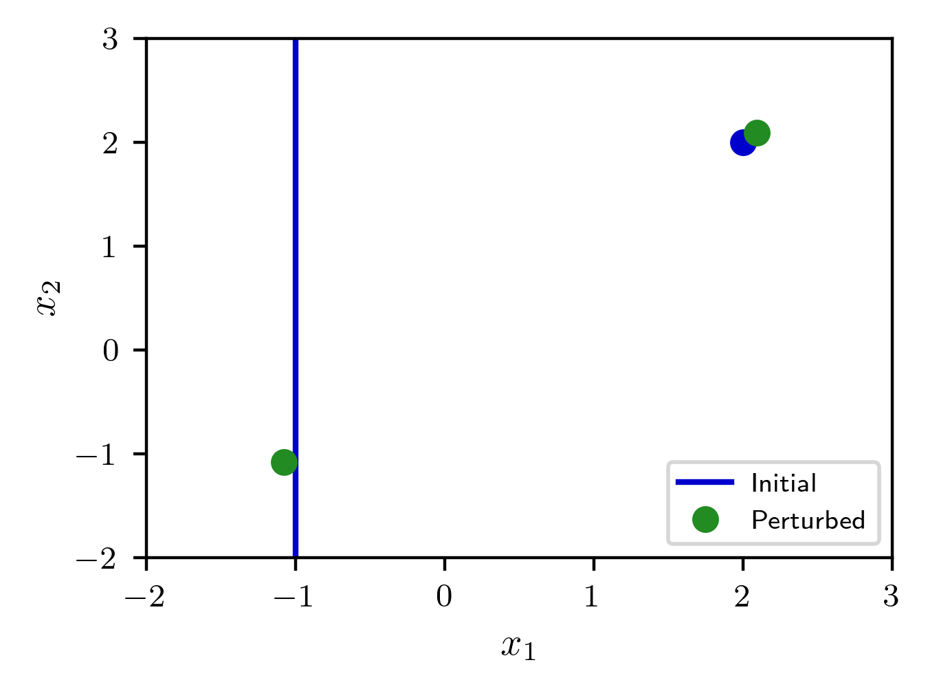
Figure 1: Solution sets for the initial and perturbed parameters

When considering witness points on a one-dimensional component, the system under consideration has the form

$$f_{R}(x;p)=\left[\begin{array}[]{c}Rf(x;p)\\ L(x)\end{array}\right]=\left[\begin{array}[]{c}x_{1}x_{2}-2x_{1}+p_{1}x_{2}+p_{2}+\Box(x_{1}^{2}-2x_{1}+p_{1}x_{1}+p_{2})\\ \Box x_{1}+\Box x_{2}+\Box\end{array}\right]$$ (14)

where each $\Box$ represents an independent random complex number with $R=[1~{}\Box]$. Solving $f_{R}(x;\hat{p})$, there is one solution for which $f(x;\hat{p})$ is far from vanishing (called a nonsolution) and one solution, call it $\hat{x}$ with $\hat{x}_{1}$ in the vicinity of $-1$, for which $f(\hat{x};\hat{p})$ is close to vanishing. Thus, we aim to recover $p^{*}$ near $\hat{p}$ for which this later point is an actual witness point for a one-dimensional line. With this, the fiber product system becomes

$$\mathcal{F}=\left[\begin{array}[]{c}x_{1}x_{2}-2x_{1}+p_{1}x_{2}+p_{2}\\ x_{1}^{2}-2x_{1}+p_{1}x_{1}+p_{2}\\ c_{1}x_{1}+c_{2}x_{2}+c_{3}\end{array}\right]$$ (15)

and the critical point system using homogenized Lagrange multipliers yields

$$\mathcal{G}=\left[\begin{array}[]{c}x_{1}x_{2}-2x_{1}+p_{1}x_{2}+p_{2}\\ x_{1}^{2}-2x_{1}+p_{1}x_{1}+p_{2}\\ c_{1}x_{1}+c_{2}x_{2}+c_{3}\\ \lambda_{1}(x_{2}-2)+\lambda_{2}(2x_{1}+p_{1}-2)+\lambda_{3}c_{1}\\ \lambda_{1}(x_{1}+p_{1})+\lambda_{3}c_{2}\\ \lambda_{0}(p_{1}-\hat{p}_{1})+\lambda_{1}x_{2}+\lambda_{2}x_{1}\\ \lambda_{0}(p_{2}-\hat{p}_{2})+\lambda_{1}+\lambda_{2}\\ \end{array}\right].$$ (16)

With $(\hat{x},\hat{p})$, tracking a single path with a gradient descent homotopy (7) recovers a nearby parameter $p^{*}$ listed in Table 3 to four decimal places. Recomputing a numerical irreducible decomposition for $f(x;p^{*})$ yields a line and an isolated point as requested.

Table 3: Initial (exact), perturbed (4 decimals), and recovered (4 decimals) parameter values

Parameter	Initial ($\tilde{p}$)	Perturbed ($\hat{p}$)	Recovered ($p^{*}$)
$p_{1}$	1	0.9876	1.0992
$p_{2}$	–2	–2.2542	–2.1984

We repeated this process by sampling 500 points from a bivariate Gaussian distribution centered at the initial parameter values $\tilde{p}=(1,-2)$ with covariance matrix $\Sigma=0.1^{2}I_{2}$ where each sample represents parameter values with error. In Fig. 2, the aforementioned $\tilde{p}$ is shown as a square, and $\hat{p}$ and $p^{*}$ are triangles, while the additional sampled values and recovered parameters are shown as circles. For this simple problem, it is easy to verify that all recovered parameter values lie along the line $V(2p_{1}+p_{2})$.

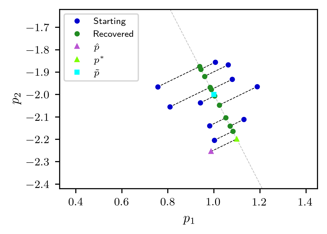
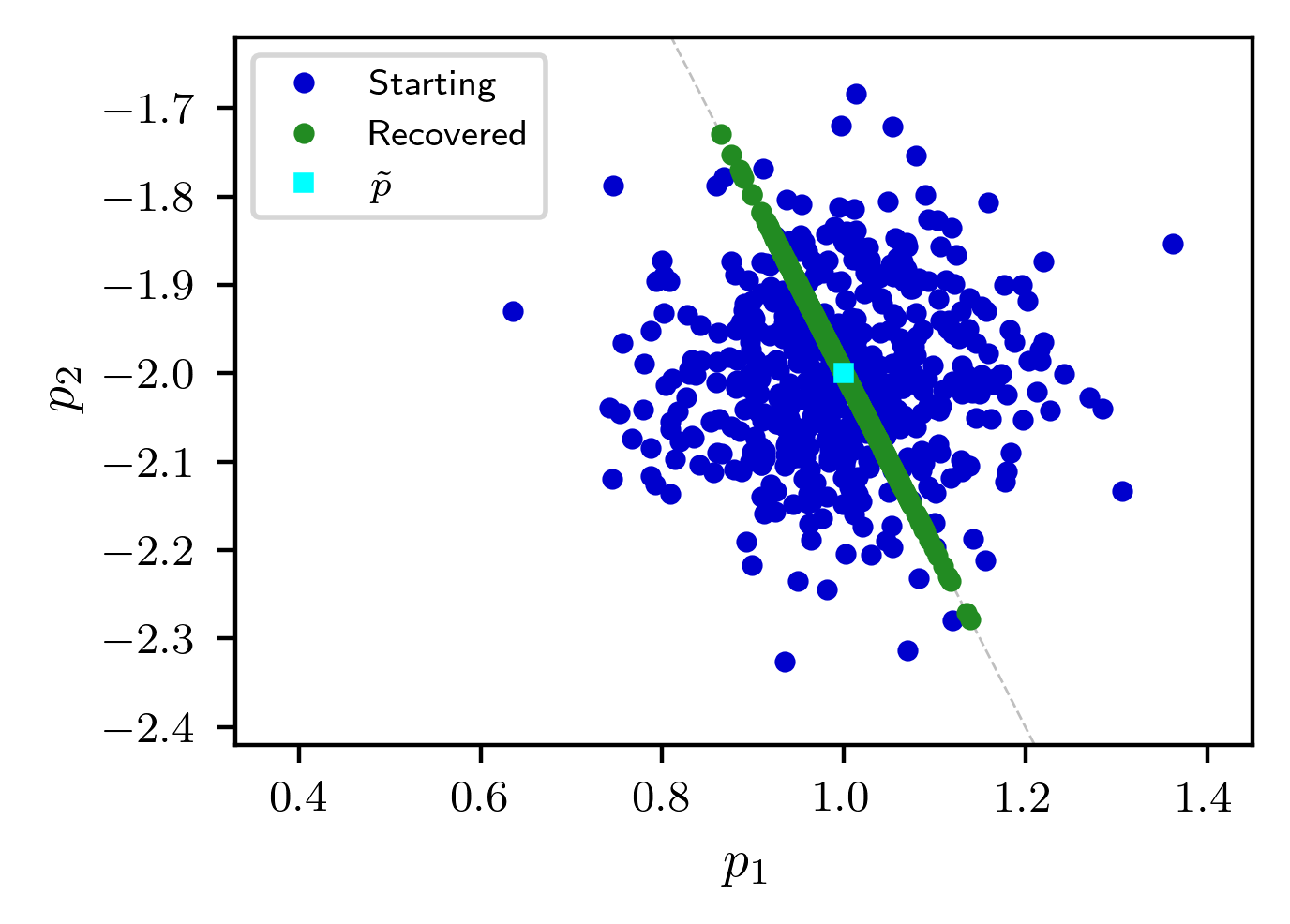
(a)	(b)

Figure 2: (a) Illustration of recovering parameters for various perturbations including the example summarized in Table 3; (b) Illustration using 500 samples

To visualize marginal histograms of the recovered parameter values from the $500$ samples, Fig. 3 shows the $p_{1}$ and $p_{2}$ coordinates along with an intrinsic coordinate parameterizing the line with $0$ corresponding to $\tilde{p}=(1,-2)$.

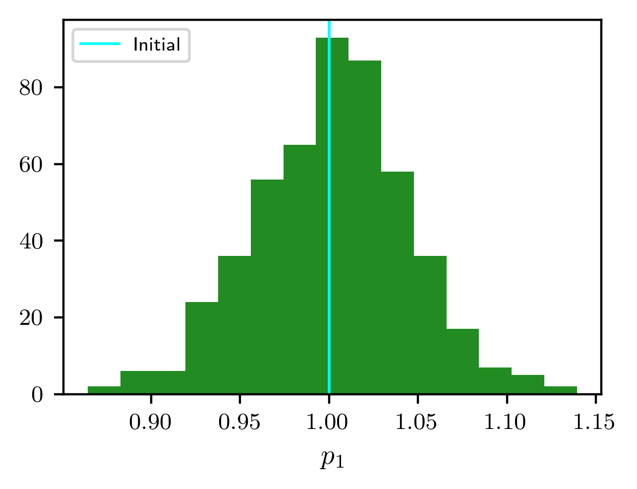
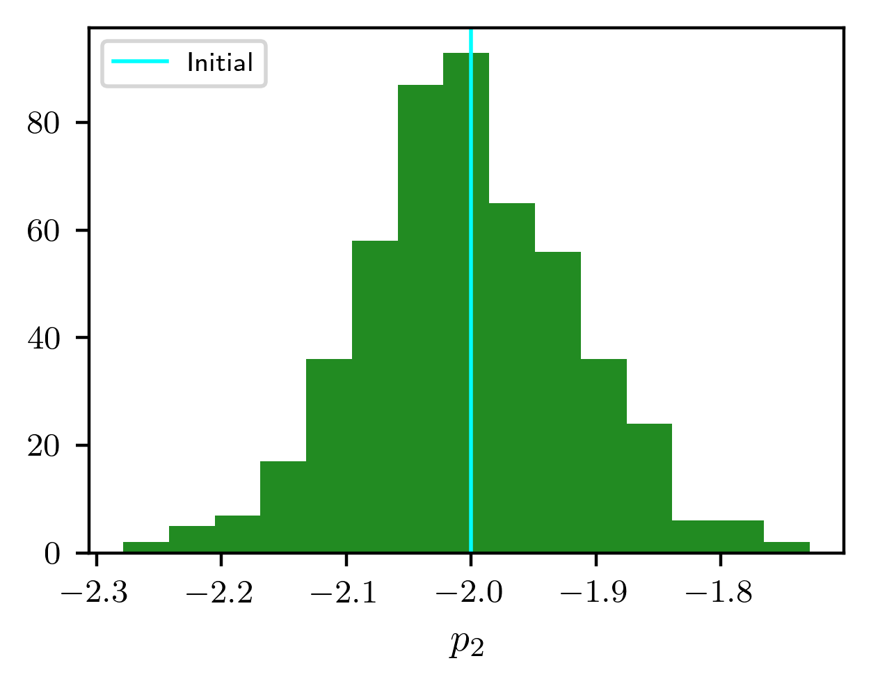
(a)	(b)	(c)

Figure 3: Histograms for (a) $p_{1}$, (b) $p_{2}$, and (c) intrinsic parameterizing coordinate for recovered parameter values from $500$ samples

For a standard multivariate Gaussian, all marginals are Gaussian. So, if we orthogonally project a multivariate Gaussian centered at $\tilde{p}$ onto a linear space passing through $\tilde{p}$, this will yield a Gaussian distribution in the linear space. In the case presented here, the perturbations from the initial parameters are both generated as zero-mean with standard deviation $0.1$, so the recovered parameters along the line should be centered on the initial parameters with that same standard deviation. Figure 3(c) is consistent with that expectation. Moreover, orthogonally projecting the distribution of the perturbed parameters onto the line perpendicular to $V(2p_{1}+p_{2})$ will also be distributed as Gaussian with standard deviation $0.1$. If one were given just the perturbed parameters and their accuracy, described as a statistical distribution, one could calculate a confidence in the null hypothesis that the given parameters are drawn from a distribution centered on an initial value for which $V(f(x;\tilde{p}))$ has one component that is a line. In this case of a single remaining degree of freedom in parameter space, a $Z$-score for $||\hat{p}-p^{*}||$ would be informative.

We will not delve into statistical analyses for more general cases. Nevertheless, we remark that if the exceptional set in parameter space is codimension $s$ and the incoming parameters are perturbed from the exceptional set with a normal distribution ${\mathcal{N}}(0,\sigma^{2}I)$, then the squared distance $\sigma^{-2}||\hat{p}-p^{*}||^{2}$ is a chi-squared distribution with $s$ degrees of freedom. (This assumes that the exceptional set is locally smooth and $\sigma$ is small enough that a local linearization of the exceptional set is accurate on the scale of $\sigma$.) If the perturbations have a more general normal distribution, say ${\mathcal{N}}(0,\Sigma)$, then it would be appropriate to change the norm used in (6) to $(p-\hat{p})^{T}\Sigma^{-1}(p-\hat{p})$ so that we are searching for a maximum likelihood estimate. The same norm would then enter into a chi-square confidence estimate.

6 Traces and numerical irreducible decomposition

With Section 5 considering witness points, the next structure to consider applying this robust framework to is computing parameter values which have solution components that decompose into various irreducible components.

6.1 Reducibility

In a numerical irreducible decomposition, the collection of witness points is partitioned into subsets corresponding with the irreducible components. One approach for performing this decomposition is via the trace test [8, 17, 28, 42] and a key decision is to determine when the linear trace vanishes. For exact systems, this can be determined robustly by computing the linear trace to higher precision, but becomes an uncertain task for systems with error as perturbations tend to destroy reducibility.

The form of the trace test that we will employ here is the second derivative trace test from [8] as this can be employed locally. Suppose that $\{f,L_{D},W\}$ is a witness set for a pure $D$-dimensional component $X$ of $V(f)$. Since discussions about multiplicity are provided in Section 7.1, suppose that each irreducible component of $X$ has multiplicity $1$ with respect to $f$. Moreover, by replacing $f$ with a randomization, we can assume that $f:{\mathbb{C}}^{n}\rightarrow{\mathbb{C}}^{n-D}$. Let $W_{r}\subset W$ consist of $r$ points. Then, there is a pure $D$-dimensional component $X^{\prime}\subset X$ with $X^{\prime}\cap V(L_{D})=W_{r}$ if and only if, for a general $L_{D}^{\prime}:{\mathbb{C}}^{n}\rightarrow{\mathbb{C}}^{D}$ and general $\alpha\in{\mathbb{C}}^{n}$,

$$\alpha\cdot\sum_{j=1}^{r}\ddot{w}_{j}=0$$ (17)

where $\{w_{1},\dots,w_{r}\}=X^{\prime}\cap V(L_{D}^{\prime})$, and $\dot{w}_{j}$ and $\ddot{w}_{j}$ satisfy

$$\left[\begin{array}[]{c}Jf(w_{j})\\ JL_{D}^{\prime}(w_{j})\end{array}\right]\cdot\dot{w}_{j}=\left[\begin{array}[]{c}0\\ 1\end{array}\right]\hbox{~{}~{}and~{}~{}}\left[\begin{array}[]{c}Jf(w_{j})\\ JL_{D}^{\prime}(w_{j})\end{array}\right]\cdot\ddot{w}_{j}=-\left[\begin{array}[]{c}\dot{w}_{j}^{T}\cdot{{\hbox{\rm Hessian}}}(f_{1})(w_{j})\cdot\dot{w}_{j}\\ \vdots\\ \dot{w}_{j}^{T}\cdot{{\hbox{\rm Hessian}}}(f_{n-D})(w_{j})\cdot\dot{w}_{j}\\ 0\end{array}\right].$$

Thus, for chosen slices and randomizing vectors, one can utilize fiber products to recover reducibility of a component of degree $r$.

Corollary 6.1.

With the setup described above, Thm. 3.1 holds when applied to

$$F_{c}(x_{1},\dot{x}_{1},\ddot{x}_{1},\dots,x_{r},\dot{x}_{r},\ddot{x}_{r},p)=\left[\begin{array}[]{c}f(x_{1};p)\\ L_{c}(x_{1})\\ \left[\begin{array}[]{c}Jf(x_{1};p)\\ JL_{c}(x_{1})\end{array}\right]\cdot\dot{x}_{1}-\left[\begin{array}[]{c}0\\ 1\end{array}\right]\\ \left[\begin{array}[]{c}Jf(x_{1};p)\\ JL_{c}(x_{1})\end{array}\right]\cdot\ddot{x}_{1}+\left[\begin{array}[]{c}\dot{x}_{1}^{T}\cdot{{\hbox{\rm Hessian}}}(f_{1})(x_{1};p)\cdot\dot{x}_{1}\\ \vdots\\ \dot{x}_{1}^{T}\cdot{{\hbox{\rm Hessian}}}(f_{n-D})(x_{1};p)\cdot\dot{x}_{j}\\ 0\end{array}\right]\\ \vdots\\ f(x_{r};p)\\ L_{c}(x_{r})\\ \left[\begin{array}[]{c}Jf(x_{r};p)\\ JL_{c}(x_{r})\end{array}\right]\cdot\dot{x}_{r}-\left[\begin{array}[]{c}0\\ 1\end{array}\right]\\ \left[\begin{array}[]{c}Jf(x_{r};p)\\ JL_{c}(x_{r})\end{array}\right]\cdot\ddot{x}_{r}+\left[\begin{array}[]{c}\dot{x}_{r}^{T}\cdot{{\hbox{\rm Hessian}}}(f_{1})(x_{r};p)\cdot\dot{x}_{r}\\ \vdots\\ \dot{x}_{r}^{T}\cdot{{\hbox{\rm Hessian}}}(f_{n-D})(x_{r};p)\cdot\dot{x}_{r}\\ 0\end{array}\right]\\ \alpha_{c}\cdot(\ddot{x}_{1}+\cdots+\ddot{x}_{r})\end{array}\right]$$

where $c$ contains the coefficients of $L_{c}:{\mathbb{C}}^{n}\rightarrow{\mathbb{C}}^{D}$ and $\alpha_{c}\in{\mathbb{C}}^{n}$.

For perturbed parameter values $\hat{p}$, one is looking for collections of points for which (17) is close to $0$. The situation in Cor. 6.1 covers the case when $X$ has degree $d$ and one is considering decomposing $X$ into a degree $r$ and degree $d-r$ component (where $1\leq r\leq d-r\leq d$). If one is considering factorization into more than two components or the factorization of components in different dimensions, then Cor. 3.3 applies with stacking fiber product systems resulting from Cor. 6.1. Moreover, in the multiplicity $1$ case considered here, Remark 3.4 applies.

6.2 Illustrative example

Consider the parameterized family of polynomial systems

$$f(x;p)=p_{1}+p_{2}x_{1}+p_{3}x_{1}^{2}+p_{4}x_{1}^{3}+p_{5}x_{1}x_{2}+p_{6}x_{1}^{2}x_{2}+p_{7}x_{1}^{3}x_{2}+p_{8}x_{2}^{2}+p_{9}x_{1}^{2}x_{2}^{2}+p_{10}x_{1}x_{2}^{3}$$ (18)

from [53]. For generic $p\in{\mathbb{C}}^{10}$, $f(x;p)=0$ defines a quartic plane curve. The problem described in [53, Ex. 2] considers the parameters $\tilde{p}=(-30,20,18,-12,12,-8,0,-5,3,2)$ with perturbation $\hat{p}=(-30,20,18,-12,12.000007,-8,0.0000003,-5,3,2)$ so that

$$f(x;\tilde{p})=(3x_{1}^{2}+2x_{1}x_{2}-5)(x_{2}^{2}-4x_{1}+6)\hbox{~{}~{}and~{}~{}}f(x;\hat{p})=f(x;\tilde{p})+0.0000003x_{1}^{3}x_{2}+0.000007x_{1}x_{2}$$

with the corresponding quartic plane curves illustrated in Fig. 4.

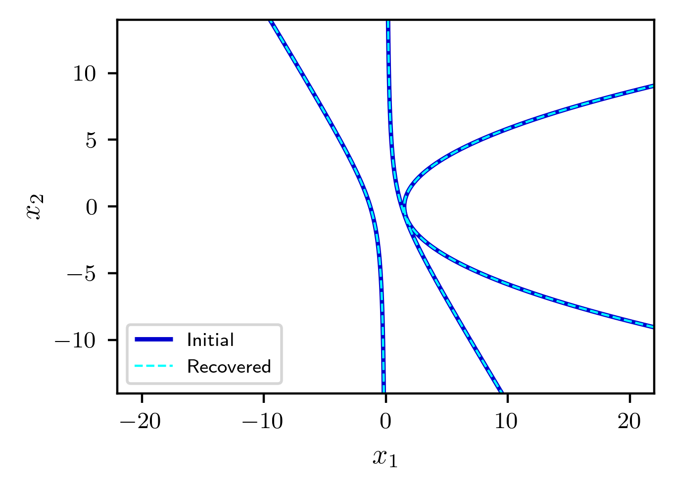
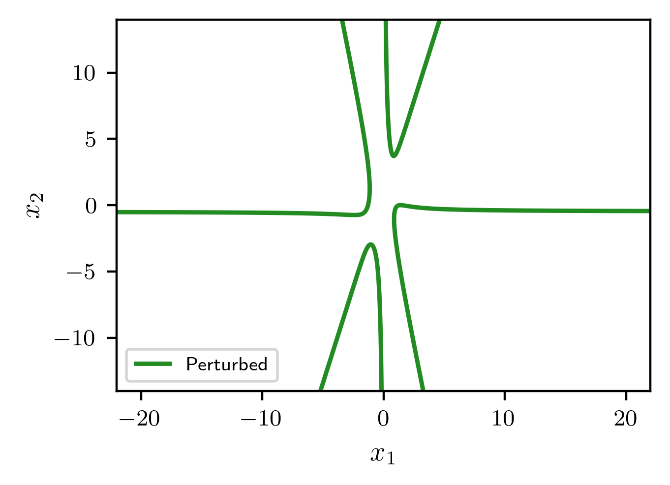
(a)	(b)

Figure 4: Solution sets corresponding to the (a) initial and recovered parameters, and (b) perturbed parameters

For illustration, Table 4 considers the result of intersecting $f(x;\hat{p})=0$ with the linear space defined by $2x_{1}-3x_{2}=1$. Clearly, we see that both $\ddot{w}_{1}+\ddot{w}_{2}$ and $\ddot{w}_{3}+\ddot{w}_{4}$ are close to zero indicating that we should consider computing parameters $p^{*}$ near $\hat{p}$ for which $f(x;p^{*})$ factors into two quadratics via the second derivative trace test, i.e., apply Cor 6.1 with $r=2$.

Table 4: Summary of solutions (8 decimals) satisfying $f(x;\hat{p})=2x_{1}-3x_{2}-1=0$

$j$	$w_{j}$	$\dot{w_{j}}$	$\ddot{w}_{j}$
$1$	$\begin{array}[]{r}1.15384590\\ 0.43589727\end{array}$	$\begin{array}[]{r}0.08241763\\ -0.27838824\end{array}$	$\begin{array}[]{r}0.00546655\\ 0.00364437\end{array}$
$2$	$\begin{array}[]{r}-0.99999993\\ -0.99999995\end{array}$	$\begin{array}[]{r}0.07142858\\ -0.28571428\end{array}$	$\begin{array}[]{r}-0.00546648\\ -0.00364432\end{array}$
$3$	$\begin{array}[]{r}1.64589862\\ 0.76393241\end{array}$	$\begin{array}[]{r}-0.17082057\\ -0.44721371\end{array}$	$\begin{array}[]{r}0.13416408\\ 0.08944272\end{array}$
$4$	$\begin{array}[]{r}8.35410056\\ 5.23606704\end{array}$	$\begin{array}[]{r}1.17082044\\ 0.44721363\end{array}$	$\begin{array}[]{r}-0.13416415\\ -0.08944277\end{array}$

Utilizing Remark 3.4, Table 5 shows the corresponding dimension of parameter space based on the number of component systems utilized. In this case, one sees a stabilization of the dimension of the parameter space to $6$ using $4$ component systems. That is, we expect to recover parameters $p^{*}$ contained in a $6$-dimensional parameter space. The resulting gradient descent homotopy (7) with homogenized Lagrange multipliers is a square system consisting of the same number of variables and equations which is also listed in Table 5. Finally, Table 5 also records the numerical irreducible decomposition of $f(x;p^{*})$ for the corresponding recovered $p^{*}$. This column also indicates that $4$ component systems are needed with the recovered parameters (to $7$ decimal places) provided in Table 6. For comparison, written using double precision, the recovered factorization from [53] and $p^{*}$ is provided in Table 7. The key difference is that [53] enforced $p_{7}=0$ so that the third factor maintained the same monomial structure as the exact system while the second derivative trace test only enforced factorability. Hence, with the additional constraint, the recovered factorization in [53] is further away ($3.76\cdot 10^{-6}$) from $p^{*}$ than $\hat{p}$ ($3.15\cdot 10^{-6}$). Of course, one could impose the additional parameter space condition, namely, $p_{7}=0$, with the second derivative trace test approach and recover the same factorization as [53].

Table 5: Summary for different component systems

Component Systems	Dimension	System Size	Recovered Components
1	9	35	One component of degree 4
2	8	60	One component of degree 4
3	7	85	One component of degree 4
4	6	110	Two components of degree 2
5	6	135	Two components of degree 2

Table 6: Initial (exact), perturbed (exact), and recovered (7 decimals) parameter values

Parameter	Initial ($\tilde{p}$)	Perturbed ($\hat{p}$)	Recovered ($p^{*}$)
$p_{1}$	–30	–30.0000000	–30.0000003
$p_{2}$	20	20.0000000	19.9999994
$p_{3}$	18	18.0000000	18.0000003
$p_{4}$	–12	–12.0000000	–11.9999997
$p_{5}$	12	12.0000070	12.0000057
$p_{6}$	–8	–8.0000000	–8.0000019
$p_{7}$	0	0.0000003	–0.0000014
$p_{8}$	–5	–5.0000000	–5.0000002
$p_{9}$	3	3.0000000	2.9999992
$p_{10}$	2	2.0000000	2.0000006

Table 7: Comparison of factors (double precision)

Factors from [53]	$-30.0000005908641$
	$1-0.600000000000000x_{1}^{2}-0.400000158490569x_{1}x_{2}$
	$1-0.666666625730982x_{1}+0.166666656432746x_{2}^{2}$
Factors from $p^{*}$	$-30.0000003490653$
	$1-0.600000003568289x_{1}^{2}-0.400000104966183x_{1}x_{2}$
	$1-0.666666639555509x_{1}+0.166666672330951x_{2}^{2}-7.87997843076905\cdot 10^{-8}x_{1}x_{2}$

7 Multiplicity and local Hilbert function

The final structure we consider for applying this robust framework to is to compute parameter values which have solutions with specified multiplicity and local Hilbert function.

7.1 Macaulay matrix

For a univariate polynomial $u(x)$, a number $x^{*}$ is said to have multiplicity $\mu\geq 0$ if and only if $u(x^{*})=u^{\prime}(x^{*})=u^{\prime\prime}(x^{*})=\cdots=u^{(\mu-1)}(x^{*})=0$ and $u^{(\mu)}(x^{*})\neq 0$. For a multivariate polynomial system, derivatives are replaced with partial derivatives leading to different ways of having a solution with multiplicity $\mu$. One approach for computing multiplicity in multivariate systems is via Macaulay matrices first introduced in [31] and utilized in various methods such as [3, 11, 15, 16, 46, 51, 54] to name a few.

For $\alpha\in{\mathbb{Z}}_{\geq 0}^{n}$, define

$$|\alpha|=\alpha_{1}+\cdots+\alpha_{n},~{}~{}~{}\alpha!=\alpha_{1}!\cdots\alpha_{n}!,~{}~{}~{}\hbox{and}~{}~{}~{}\partial_{\alpha}=\frac{1}{\alpha!}\frac{\partial^{|\alpha|}}{\partial x^{\alpha}}.$$

For $x^{*}\in{\mathbb{C}}^{n}$, consider the linear functional $\partial_{\alpha}[x^{*}]$ from polynomials in $x$ to ${\mathbb{C}}$ defined by

$$\partial_{\alpha}[x^{*}](g)=(\partial_{\alpha}g)(x^{*})$$

which is simply the coefficient of $(x-x^{*})^{\alpha}$ in an expansion of $g(x)$ about $x^{*}$. For a polynomial system $f:{\mathbb{C}}^{n}\rightarrow{\mathbb{C}}^{k}$ and $d\in{\mathbb{Z}}_{\geq 0}$, the $d^{\rm th}$ Macaulay matrix of $f$ at $x^{*}$ is

$$M_{d}(f,x^{*})=\left[\partial_{\alpha}[x^{*}]\left((x-x^{*})^{\beta}f_{j}\right)\hbox{~{}~{}such that~{}~{}}|\alpha|\leq d,|\beta|\leq\max\{0,d-1\},j=1,\dots,k\right]$$

where the rows are indexed by $(\beta,j)$ while the columns are indexed by $\alpha$. Define $\beta\leq\alpha$ if $\beta_{a}\leq\alpha_{a}$ for all $a=1,\dots,n$. By Leibniz rule,

$$\partial_{\alpha}[x^{*}]\left((x-x^{*})^{\beta}f_{j}\right)=\left\{\begin{array}[]{ll}\partial_{\alpha-\beta}[x^{*}](f_{j})&\hbox{~{}if~{}}\beta\leq\alpha,\\ 0&\hbox{~{}otherwise.}\end{array}\right.$$

For example, $M_{0}(f,x^{*})=f(x^{*})$ and $M_{1}(f,x^{*})=\left[f(x^{*})~{}~{}Jf(x^{*})\right]$. Moreover, there are matrices $A_{d}(f,x^{*})$ and $B_{d}(f,x^{*})$ such that

$$M_{d+1}(f,x^{*})=\left[\begin{array}[]{cc}M_{d}(f,x^{*})&A_{d}(f,x^{*})\\ 0&B_{d}(f,x^{*})\end{array}\right].$$ (19)

The local Hilbert function of $f$ at $x^{*}$ is

$$h_{f,x^{*}}(d)=\dim{{\hbox{\rm null~{}}}}M_{d}(f,x^{*})-\dim{{\hbox{\rm null~{}}}}M_{d-1}(f,x^{*})$$

where one defines $\dim{{\hbox{\rm null~{}}}}M_{-1}(f,x^{*})=0$. In particular, $x^{*}\in V(f)$ if and only if $h(0)=1$. Moreover, if $x^{*}\in V(f)$, then $x^{*}$ is isolated in $V(f)$ if and only if there exists $d^{*}\geq 0$ such that $h_{f,x^{*}}(d)=0$ for all $d>d^{*}$ with multiplicity $\mu=\dim{{\hbox{\rm null~{}}}}M_{d^{*}}(f,x^{*})=\sum_{d=0}^{d^{*}}h_{f,x^{*}}(d)$. Such a statement was used in [3, 51] to construct a local approach to decide if $x^{*}\in V(f)$ was isolated or not.

The following shows how to impose a local Hilbert function condition.

Corollary 7.1.

With the setup described above, let $d\in{\mathbb{Z}}_{\geq 0}$ and $x^{*}\in{\mathbb{C}}^{n}$. If $h_{f,x^{*}}(0)=1$ and $h_{f,x^{*}}(j)\in{\mathbb{Z}}_{\geq 1}$ for $j=1,\dots,d$, then $f(x^{*})=0$ and, for generic square unitary matrices $R_{1},\dots,R_{d}$ of appropriate sizes, the following collection of linear systems defined in terms of matrices $\Sigma_{j}$ and $\Lambda_{j}$ has a unique solution for all $j=1,\dots,d$:

$$\left[\begin{array}[]{cc}M_{j-1}(f,x^{*})&A_{j-1}(f,x^{*})\\ 0&B_{j-1}(f,x^{*})\end{array}\right]\cdot\left[\begin{array}[]{c}\Sigma_{j}\\ R_{j}\left[\begin{array}[]{c}\Lambda_{j}\\ I_{h(j)}\end{array}\right]\end{array}\right]=0$$ (20)

where $h(j)=h_{f,x^{*}}(j)$ and $I_{a}$ is the $a\times a$ identity matrix.

Proof.

The result follows immediately from (19), the definition of the local Hilbert function, and [4, Thm. 2]. In particular, the matrix $R_{j}\left[\begin{array}[]{c}\Lambda_{j}\\ I_{h(j)}\end{array}\right]$ has rank $h(j)=h_{f,x^{*}}(j)$ and thus (20) yields $h(j)$ independent null vectors that are not contained in the null space of $M_{j-1}(f,x^{*})$ as required. Uniqueness follows from [4, Thm. 2] where the total number of unknowns in $\Sigma_{j}$ and $\Lambda_{j}$ is precisely the dimension of the corresponding Grassmannian. ∎

In order to enforce various local Hilbert functions separately at several points, Cor. 7.1 can be applied individually for each point and then all such systems can be collected together. To enforce multiplicity of a component, one applies a local Hilbert function condition at each of the witness points separately with respect to the polynomial system and slicing system together. Then, one simply takes fiber products resulting from the component systems in Cor. 7.1 stacked together via Thm. 3.1 and Cor. 3.3. Additionally, if one aims to enforce a Hilbert function of a zero-scheme, this approach can naturally be generalized following [15].

For perturbed parameter values $\hat{p}$, one is looking for solutions to $f(x;\hat{p})=0$ for which the corresponding Macaulay matrices are nearly rank deficient. This can be determined using numerical rank revealing methods such as the singular value decomposition to determine appropriate null space conditions to apply.

7.2 Illustrative example

Similar to Section 5.2, computing a numerical irreducible decomposition of

$$f(x;p)=\left[\begin{array}[]{c}f_{1}\\ f_{2}\end{array}\right]=\left[\begin{array}[]{c}x_{1}^{3}-2p_{1}x_{1}^{2}-2x_{1}^{2}+p_{1}^{2}x_{1}+4p_{1}x_{1}-p_{1}^{2}-p_{2}\\ x_{1}^{2}x_{2}-2x_{1}^{2}-2p_{1}x_{1}x_{2}+4p_{1}x_{1}+p_{1}^{2}x_{2}-p_{1}^{2}-p_{2}\end{array}\right],$$ (21)

with $\tilde{p}=(1,1)$, has a line and an isolated point in the solution space. However, for this system, the line has multiplicity two. When these parameters are perturbed, say with $\mathcal{N}(0,0.1^{2})$ error yielding $\hat{p}=(1.2346,1.0089)$ to 4 decimal places, the point and line structure breaks into three isolated points. In this case, we want to recover nearby parameters giving the special structure of a one-dimensional line with multiplicity two and an isolated point. As in Section 5.2, we randomize to a single equation and add a slice. After solving

$$f_{R}(x;p)=\left[\begin{array}[]{c}Rf(x;p)\\ L(x)\end{array}\right]=\left[\begin{array}[]{c}f_{1}+\Box f_{2}\\ \Box x_{1}+\Box x_{2}+\Box\end{array}\right]=0,$$ (22)

we choose one of the two solutions near the one-dimensional line. To recover the multiplicity at this component, we add the condition outlined in Cor. 7.1. In particular, as mentioned in Section 2.6, since the randomized system having multiplicity 2 implies the original system has multiplicity 2, we simply work with the randomized system with (20) corresponding to

$$Jf_{R}(x;p)\cdot R_{1}\cdot\left[\begin{array}[]{c}\lambda\\ 1\end{array}\right]=0.$$ (23)

Hence, ${\mathcal{F}}$ consists of the polynomials in (22) and (23). Using a gradient descent homotopy (7) with homogenized Lagrange multipliers yields the recovered parameters listed in Table 8 and pictorially represented in Fig. 5.

Similar to Section 5.2, we repeated this process with 500 samples from a bivariate Gaussian distribution centered at the initial parameter values $\tilde{p}=(1,1)$ with covariance matrix $\Sigma=0.1^{2}I_{2}$. The results of this experiment are summarized in Fig. 5. For this simple problem, it is easy to verify that all recovered parameter values lie along the parabola $V(p_{1}^{2}-p_{2})$. Figure 6 shows histograms of the marginal distributions for $p_{1}$, $p_{2}$, and along an intrinsic parameterization of the tangent line to the parabola at $\tilde{p}$.

Table 8: Initial (exact), perturbed (4 decimals), and recovered (4 decimals) parameter values

Parameter	Initial ($\tilde{p}$)	Perturbed ($\hat{p}$)	Recovered ($p^{*}$)
$p_{1}$	1	1.2346	1.0479
$p_{2}$	1	1.0089	1.0980

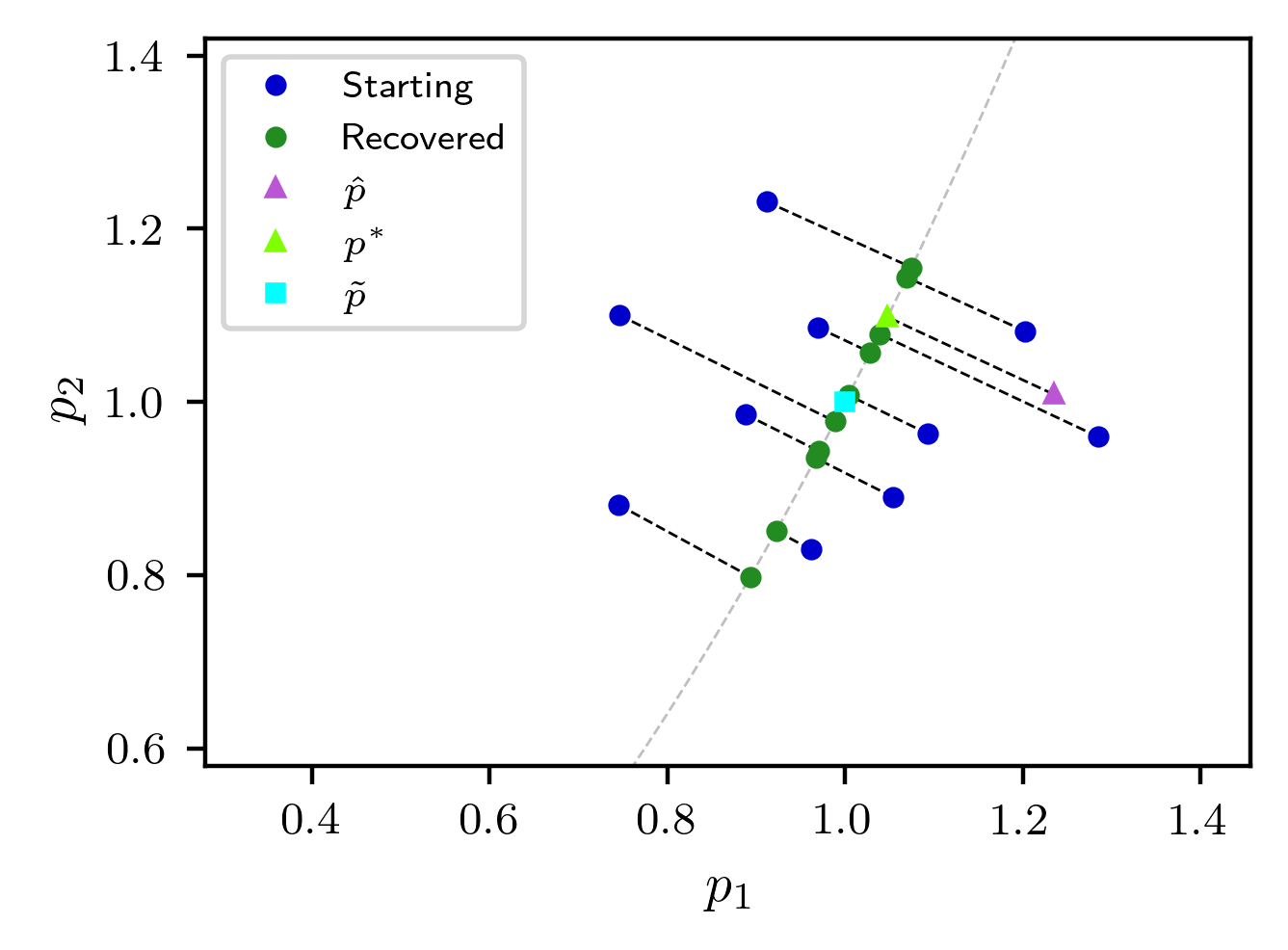
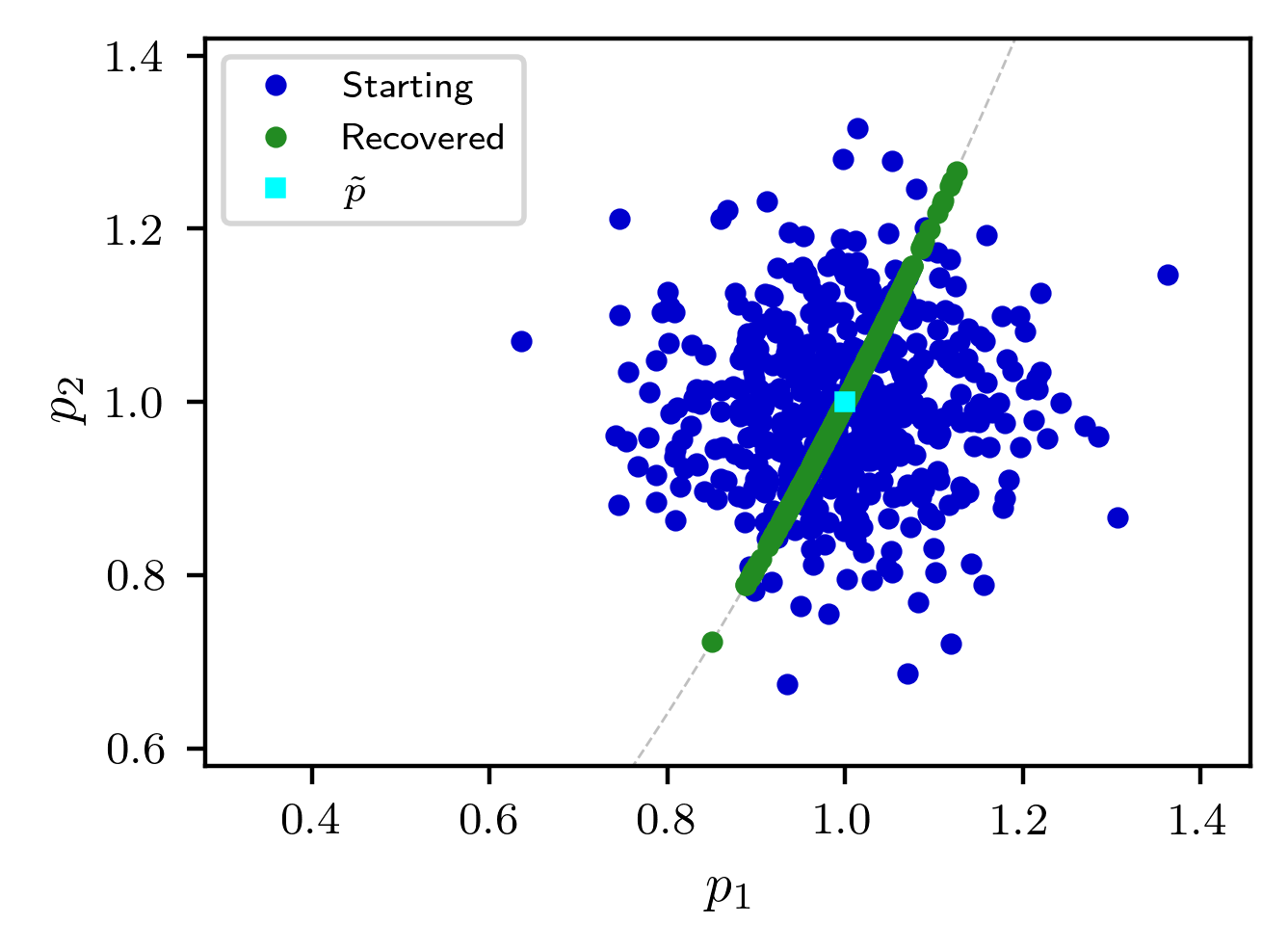
(a)	(b)

Figure 5: (a) Illustration of recovering parameters for various perturbations including the example summarized in Table 8; (b) Illustration using 500 samples

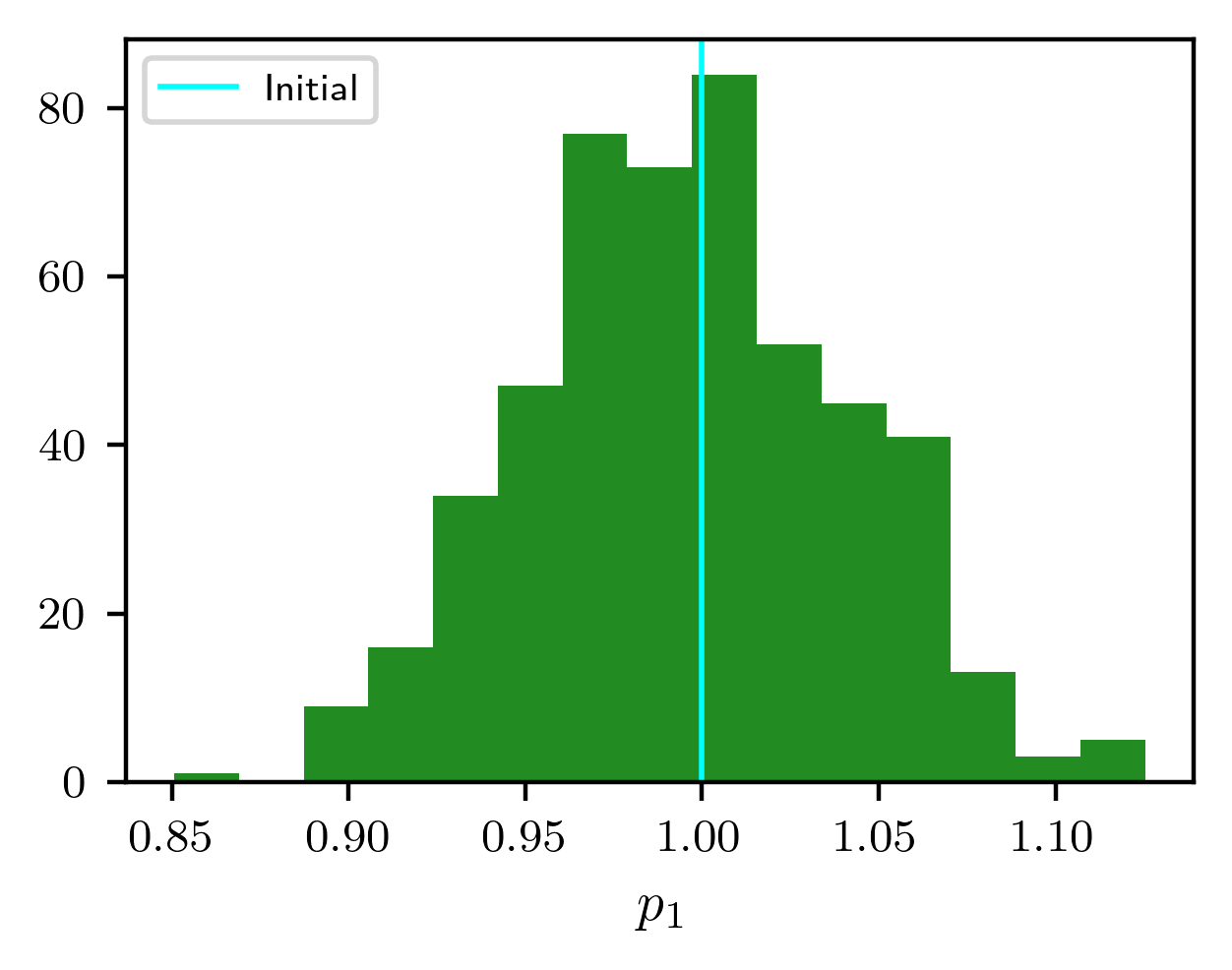
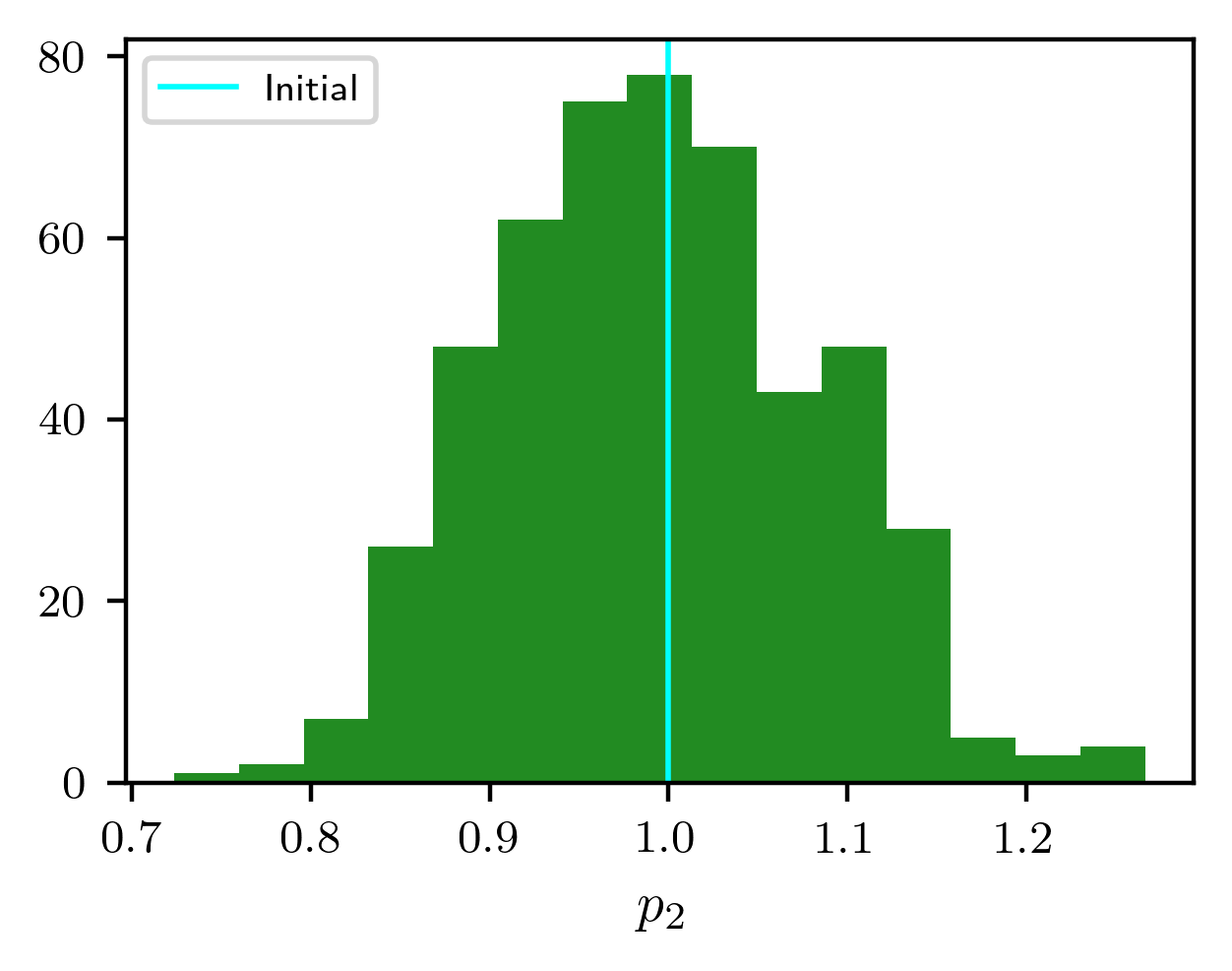
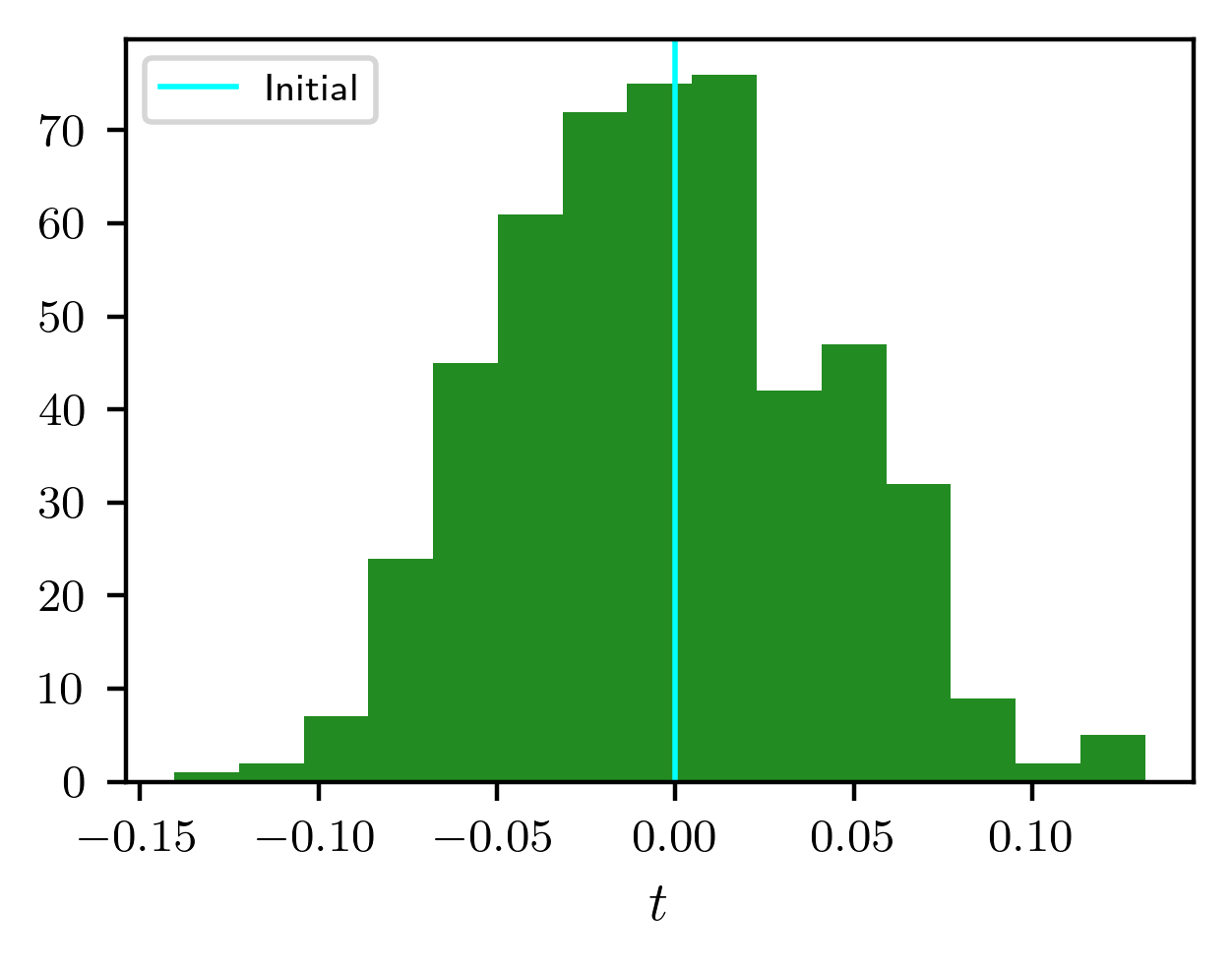
(a)	(b)	(c)

Figure 6: Histograms for (a) $p_{1}$, (b) $p_{2}$, and (c) intrinsic parameterizing coordinate along tangent line for recovered parameter values from $500$ samples

8 Kinematic examples

The examples in Sections 4–7 were designed for illustrative purposes. The following considers three examples derived from the field of kinematics.

8.1 Decomposable 4-bar coupler curve

Consider the 4-bar linkage given by the parameterized family of polynomial systems

$$f(x;p)=\left[\begin{array}[]{c}x_{1}^{2}+x_{2}^{2}-p_{1}^{2}\\ (x_{3}-p_{2})^{2}+x_{4}^{2}-p_{3}^{2}\\ (x_{1}-x_{3})^{2}+(x_{2}-x_{4})^{2}-p_{4}^{2}\end{array}\right].$$ (24)

For generic $p\in{\mathbb{C}}^{4}$, $V(f(x;p))$ is an irreducible sextic $(d=6)$ curve. It is known that $p_{1}=p_{3}$ and $p_{2}=p_{4}$ yields a parallelogram linkage and the solution set factors into a quadratic and quartic curve. Considering initial parameter values $\tilde{p}=(1,2,1,2)$, we perturbed the parameters with $\mathcal{N}(0,0.01^{2})$ error yielding $\hat{p}=(1.0025,2.0101,1.0098,2.0014)$ rounded to four decimals. For illustration, Fig. 7 shows the solution set projected into $(x_{1},x_{4})$ space.

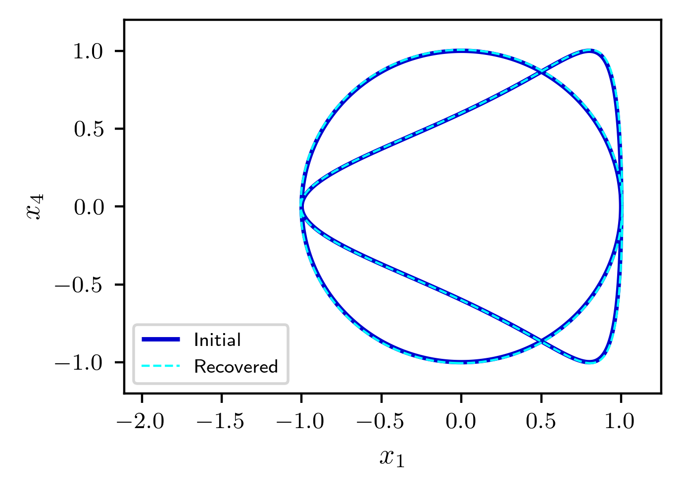
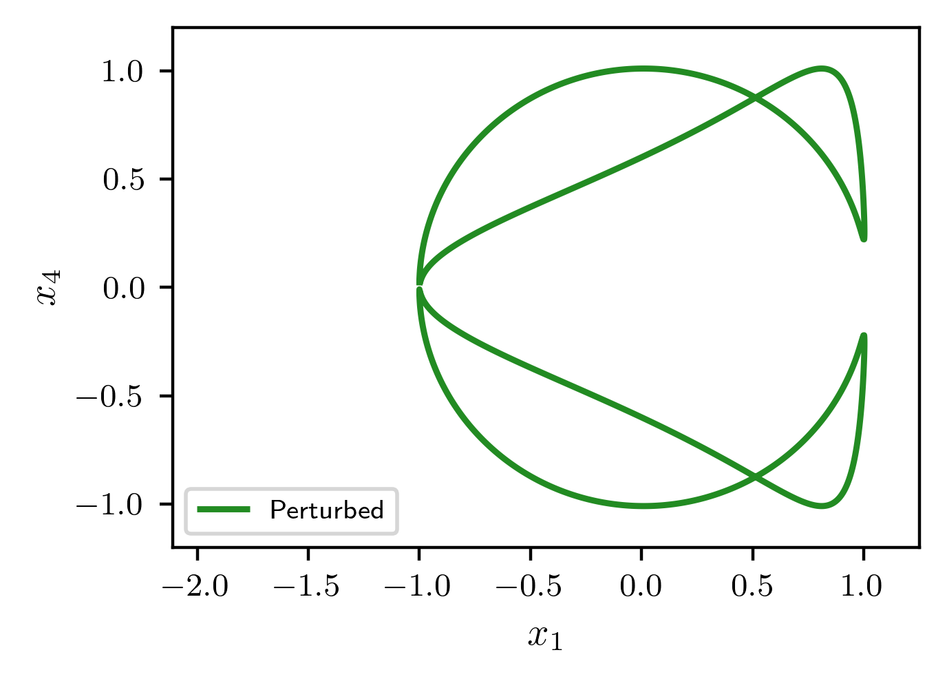
(a)	(b)

Figure 7: Projections of the 4-bar coupler curve in $(x_{1},x_{4})$ space corresponding to (a) initial and recovered parameters, and (b) perturbed parameters

For the perturbed parameter values $\hat{p}$, the sextic curve does not factor, following Section 6.2, linear traces are close to zero for collections of $r=2$ and $d-r=4$ points. Thus, we aim to apply Cor. 6.1 to recover parameters $p^{*}$ near $\hat{p}$ such that the solution set $V(f(x;p^{*}))$ factors into a quadratic curve and a quartic curve using the second derivative trace test. Table 9 summarizes the results of applying Remark 3.4 to determine the number of component systems needed, namely the dimension stabilizes with two systems. The corresponding system sizes are also reported in Table 9, where the systems are square via homogenized Lagrange multipliers. Using a gradient descent homotopy (7) with two component systems, the recovered parameters $p^{*}$ are reported in Table 10 to 4 decimals and one clearly sees the parallelogram linkage structure is recovered. The resulting decomposable solution set $V(f(x;p^{*}))$ is illustrated in Fig. 7(a).

Table 9: Dimensions and system size for different number of component systems

Component Systems	Dimension	System Size
1	3	53
2	2	102
3	2	151
4	2	200

Table 10: Initial (exact), perturbed (4 decimals), and recovered (4 decimals) parameter values

Parameter	Initial ($\tilde{p}$)	Perturbed ($\hat{p}$)	Recovered ($p^{*}$)
$p_{1}$	1	1.0025	1.0062
$p_{2}$	2	2.0101	2.0057
$p_{3}$	1	1.0098	1.0062
$p_{4}$	2	2.0014	2.0057

8.2 Stewart-Gough platform

A Stewart-Gough platform consists of two bodies, a base and an end-plate, connected by six legs as illustrated in Fig. 8. For $j=1,\ldots,6$, the $j^{\rm th}$ leg imposes a square distance $d_{j}$ between point $a_{j}\in{\mathbb{R}}^{3}$ of the base and point $b_{j}\in{\mathbb{R}}^{3}$ of the end-plate. Letting “$*$” denote quaternion multiplication and letting $v^{\prime}$ denote the quaternion conjugate of $v$, the leg constraints may be written as follows, for $j=1,\ldots,6$,

$$f_{j}(e,g;a,b,d)=(a_{j}*a_{j}^{\prime}+b_{j}*b_{j}^{\prime}-d_{j})e*e^{\prime}-e*b_{j}*e^{\prime}*a_{j}^{\prime}*a_{j}*e*b_{j}^{\prime}*e^{\prime}\\ +g*b_{j}^{\prime}*e^{\prime}+e*b_{j}*g^{\prime}-g*e^{\prime}*a_{j}^{\prime}-a_{j}*e*g^{\prime}+g*g^{\prime}=0$$ (25)

where $e,g$ are quaternions in a Study coordinate representation of the position and orientation of the end-plate. Hence, $e,g$ must satisfy the Study quadric

$$Q(e,g)=g_{0}e_{0}+g_{1}e_{1}+g_{2}e_{2}+g_{3}e_{3}=0.$$ (26)

In this example, we set $e_{0}=1$ to dehomogenize the system. For generic parameters $p=(a,b,d)$, this platform can be assembled in 40 rigid configurations over the complex numbers. That is, the solution set of the parameterized polynomial system resulting from the 6 leg constraints in (25) and Study quadratic in (26) consists of 40 isolated points. However, for $\tilde{p}$ reported in Table 12 in Appendix A derived from [18, Ex. 2.2], this platform moves in a circular motion as illustrated in Fig. 8. In particular, this circular motion corresponds to the solution set containing a quadratic curve. To apply the robustness framework, we consider a slight perturbation using $\mathcal{N}(0,(10^{-9})^{2})$ error yielding $\hat{p}$ in Table 12 for which the platform becomes rigid.

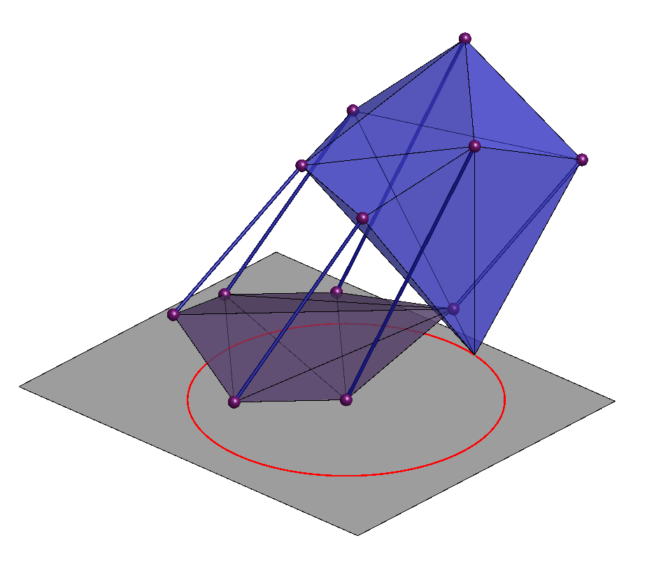
Figure 8: A Stewart-Gough platform. The $z=0$ plane (gray) contains the circular path (red) corresponding to one point of the end-plate

Following Section 5.2, we aim to find $p^{*}$ near $\hat{p}$ for which the solution set contains a quadratic curve. First, we consider a randomization of the 6 leg constraints down to 5 conditions, the Study quadric, and a linear slice, namely

$$f_{R}(e,g;p)=\left[\begin{array}[]{c}f_{1}+\Box f_{6}\\ f_{2}+\Box f_{6}\\ f_{3}+\Box f_{6}\\ f_{4}+\Box f_{6}\\ f_{5}+\Box f_{6}\\ Q\\ \Box e_{1}+\Box e_{2}+\Box e_{3}+\Box g_{0}+\Box g_{1}+\Box g_{2}+\Box g_{3}+\Box\end{array}\right].$$ (27)

For $f_{R}(e,g;\hat{p})$, there are two solutions for which the leg constraints in (25) are close to vanishing, consistent with a degree 2 component having 2 witness points, and 38 solutions which are not close to vanishing. Using Cor. 5.1 with $d=2$ to construct the fiber product system, we apply Remark 3.4 which indicates 4 component systems are needed. The dimensions and corresponding square system sizes via homogenized Lagrange multipliers are reported in Table 11. Tracking the corresponding gradient descent homotopy (7), the recovered parameter values $p^{*}$ are reported in Table 12 in Appendix A for which the corresponding Stewart-Gough platform has regained its motion.

Table 11: Dimension and system size for different number of component systems

Component Systems	Dimension	System Size
1	40	72
2	38	102
3	36	132
4	35	162
5	35	192

8.3 Family containing the 6R inverse kinematics problem

The inverse kinematics problem for six-revolute (6R) mechanisms seeks to determine all ways to assemble a loop of six rigid links connected serially by revolute joints. One formulation [35, 47] sets the problem as a member of the following parameterized system of eight quadratics using a 2-homogeneous construction:

$$f(x;a)=\left[\begin{array}[]{c}f_{0}(x;a)\\ f_{1}(x;a)\\ f_{2}(x;a)\\ f_{3}(x;a)\\ x_{1}^{2}+x_{2}^{2}-x_{0}^{2}\\[2.0pt] x_{5}^{2}+x_{6}^{2}-x_{0}^{2}\\[2.0pt] x_{3}^{2}+x_{4}^{2}-x_{9}^{2}\\[2.0pt] x_{7}^{2}+x_{8}^{2}-x_{9}^{2}\end{array}\right],$$ (28)

where $f_{j}$ has the form

$$f_{j}(x;a)=a_{j0}x_{1}x_{3}+a_{j1}x_{1}x_{4}+a_{j2}x_{2}x_{3}+a_{j3}x_{2}x_{4}+a_{j4}x_{5}x_{7}+a_{j5}x_{5}x_{8}\\ {}+a_{j6}x_{6}x_{7}+a_{j7}x_{6}x_{8}+a_{j8}x_{1}x_{9}+a_{j9}x_{2}x_{9}+a_{j10}x_{3}x_{0}+a_{j11}x_{4}x_{0}\\ {}+a_{j12}x_{5}x_{9}+a_{j13}x_{6}x_{9}+a_{j14}x_{7}x_{0}+a_{j15}x_{8}x_{0}+a_{j16}x_{0}x_{9},$$ (29)

with $x_{0}$ and $x_{9}$ as the homogenizing coordinates. In particular, this system is defined on ${\mathbb{P}}^{4}\times{\mathbb{P}}^{4}$ with corresponding variable sets $\{x_{0},x_{1},x_{2},x_{5},x_{6}\}\times\{x_{3},x_{4},x_{7},x_{8},x_{9}\}$. We dehomogenize the system by solving on the affine patches defined by $x_{1}=1$ and $x_{3}=1$.

With $a$ consisting of 68 values, we take the parameters as the $32$ values in $a$ associated with monomials that do not vanish at infinity, i.e., $V(x_{0})\cup V(x_{9})$, namely $a_{j0},\dots,a_{j7}$ for $j=0,\dots,3$. We fix as constants the $36$ values in $a$ associated with monomials that vanish at infinity, namely $a_{j8},\dots,a_{j16}$ for $j=0,\dots,3$. Table 13 in Appendix A contains the values of these constants used in the computations. For generic parameters, the resulting system has 64 finite solutions. However, for parameters that correspond with a 6R problem, the system should only have 32 finite solutions. Thus, to utilize the robustness framework, we truncated $a\in{\mathbb{C}}^{68}$ corresponding to an actual 6R problem using single precision. Hence, the constants in Table 13 are listed in single precision and the parameter values in Table 14 are listed in both single precision (corresponding to the perturbed parameters) and double precision (corresponding to the initial parameters). Solving the system with the perturbed parameter values results in $64$ points corresponding to finite solutions that are clustered into three groups: $16$ having $|x_{0}|$ close to zero, $16$ having $|x_{9}|$ close to zero, and $32$ having both $|x_{0}|$ and $|x_{9}|$ far from zero as illustrated in Fig. 9.

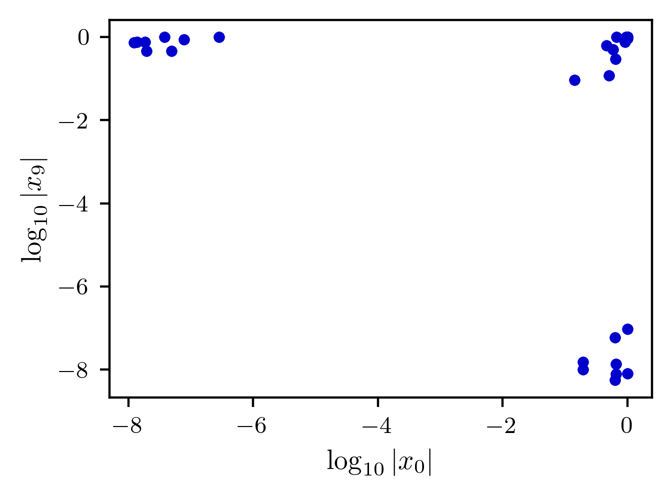
Figure 9: Logarithmic plot of absolute values of homogenizing coordinates for the $64$ solutions

First, suppose that we aim to recover parameters by forcing the $16$ solutions with $|x_{0}|$ close to zero to be at infinity, i.e., actually satisfy $x_{0}=0$. The fiber product system is constructed following Cor. 4.1. Since the solutions are not necessarily independent of each other, we utilized Remark 3.4 applied to the system with 16 component systems and observed that there were actually 4 unnecessary conditions, i.e., only 12 component systems in the fiber product are necessary, which was confirmed by a gradient descent homotopy (7).

It is the same story if one aims to recover parameters by forcing the $16$ solutions with $|x_{9}|$ close to zero to be at infinity. So, now suppose that we aim to recover parameters by forcing both sets of $16$ solutions with either $|x_{0}|$ or $|x_{9}|$ close to zero to be at infinity. Then, applying Remark 3.4, we see that these are not independent and only need $23$ fiber products. Thus, when pushing these $32$ solutions to infinity, we take $12$ for one of the infinities and only $11$ for the other. After adding homogenized Lagrange multipliers, this results in a square system of size 423. Tracking the gradient descent homotopy (7) yields the recovered parameters reported in Table 14 of Appendix A. Solving with the recovered parameters shows that all $32$ of these solutions are pushed back to infinity as illustrated in Fig. 10.

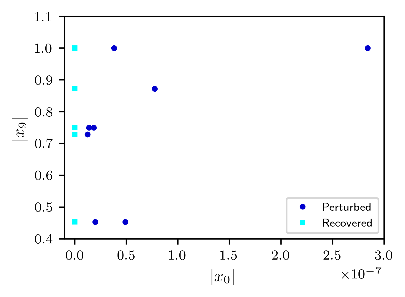
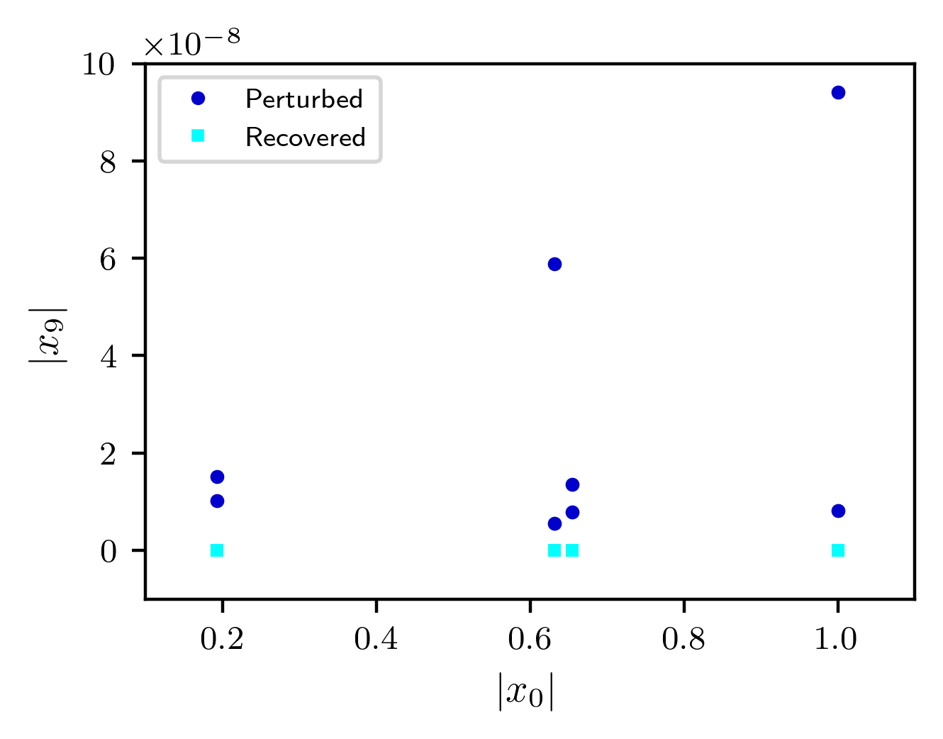
(a)	(b)

Figure 10: Absolute values of the homogenizing coordinates for (a) $16$ solutions associated with $x_{0}=0$ and (b) $16$ solutions associated with $x_{9}=0$

9 Conclusion

After proposing a framework for robustness in numerical algebraic geometry based on fiber products, this framework was applied to a collection of scenarios including fewer finite solutions, existence of higher-dimensional components, components that further decompose into irreducible components, and solution sets of higher multiplicity. For the cases considered here, with information about the questionable structural element already identified, local optimization techniques applied to fiber products produced nearby points in parameter space where the special structure exists. Moreover, in all of the examples presented here, we aimed to recover real parameter values using a gradient descent homotopy based on homogenized Lagrange multipliers associated with the Euclidean distance. For nonreal parameter values, one can utilize isotropic coordinates. Also, there are many other optimization approaches one may use to recover parameter values on exceptional sets and these other approaches could expand the size of the local convergence zone possibly allowing to recover parameters from larger perturbations. Finally, one can adjust the distance metric used such as one based on knowledge about the relative size of the parameters and their uncertainties.

Figures 3 and 6 provide histograms of the recovered parameters arising from perturbations centered at a parameter value on an exceptional set. As described in Section 5.2, perturbations using a Gaussian distribution will yield a Gaussian distribution when projecting onto a linear space. When projecting onto a nonlinear space, such as in Section 7.2, this yields approximately a Gaussian distribution on the tangent space. Further statistical analysis regarding recovered parameters is warranted.

Finally, we note that the codimension of an exceptional set in parameter space may be less than the number of conditions one seeks to impose on the solution set. For example, in the 6R problem of Section 8.3, one might naively expect the exceptional set for sending 32 points to infinity to be codimension 32, but in fact, it is codimension 23. While we have found this result numerically, it raises the more general question of how such results can be understood using the tools of algebraic geometry.

Appendix A Appendix

The following provides tables associated with Sections 8.2 and 8.3.

Table 12: Initial (exact), perturbed (12 decimals), and recovered (12 decimals) parameters

Parameter	Initial $(\tilde{p})$	Perturbed $(\hat{p})$	Recovered $(p^{*})$
$a_{1_{x}}$	0.0000	0.000000000251	0.000000000320
$a_{1_{y}}$	0.0000	0.000000001013	0.000000000982
$a_{1_{z}}$	0.0000	0.000000000980	0.000000000477
$b_{1_{x}}$	0.0000	–0.000000000200	–0.000000000269
$b_{1_{y}}$	0.0000	–0.000000000637	–0.000000000606
$b_{1_{z}}$	1.5000	1.499999998979	1.499999999482
$d_{1}$	3.2500	3.249999999891	3.249999999724
$a_{2_{x}}$	1.0000	1.000000000136	1.000000000272
$a_{2_{y}}$	0.0000	–0.000000000753	–0.000000001236
$a_{2_{z}}$	0.2500	0.249999998300	0.249999998434
$b_{2_{x}}$	1.0000	1.000000001806	1.000000001671
$b_{2_{y}}$	0.0000	–0.000000000886	–0.000000000402
$b_{2_{z}}$	1.0000	0.999999999658	0.999999999525
$d_{2}$	1.5625	1.562499999151	1.562499999240
$a_{3_{x}}$	1.0000	0.999999999712	0.999999999839
$a_{3_{y}}$	1.0000	0.999999999733	0.999999999918
$a_{3_{z}}$	0.0000	0.000000000109	–0.000000000010
$b_{3_{x}}$	1.0000	0.999999998769	0.999999998641
$b_{3_{y}}$	1.0000	0.999999999125	0.999999998940
$b_{3_{z}}$	1.5000	1.499999999413	1.499999999531
$d_{3}$	3.2500	3.250000000389	3.250000000350
$a_{4_{x}}$	–0.5000	–0.500000000115	–0.499999999750
$a_{4_{y}}$	0.5000	0.500000000098	0.500000000171
$a_{4_{z}}$	0.0000	0.000000000167	0.000000000893
$b_{4_{x}}$	–0.5000	–0.499999998762	–0.499999999127
$b_{4_{y}}$	0.5000	0.499999999424	0.499999999351
$b_{4_{z}}$	1.0000	1.000000000799	1.000000000073
$d_{4}$	2.0000	2.000000000415	2.000000000779
$a_{5_{x}}$	0.5000	0.500000000717	0.499999999761
$a_{5_{y}}$	1.5000	1.500000000939	1.500000000405
$a_{5_{z}}$	0.0000	0.000000000105	0.000000000622
$b_{5_{x}}$	0.5000	0.499999998819	0.499999999776
$b_{5_{y}}$	1.5000	1.499999999660	1.500000000194
$b_{5_{z}}$	1.0000	0.999999999603	0.999999999086
$d_{5}$	2.0000	1.999999998435	1.999999998693
$a_{6_{x}}$	–0.2500	–0.250000000190	–0.249999999931
$a_{6_{y}}$	1.2500	1.249999999364	1.250000000155
$a_{6_{z}}$	0.2500	0.250000002270	0.250000001515
$b_{6_{x}}$	–0.2500	–0.249999999033	–0.249999999292
$b_{6_{y}}$	1.2500	1.250000001020	1.250000000228
$b_{6_{z}}$	1.0000	0.999999999682	1.000000000437
$d_{6}$	1.5625	1.562500000179	1.562499999676

Table 13: Constant values truncated to single precision

Constant	Single Precision	Constant	Single Precision
$a_{08}$	7.4052387$\cdot$10-2	$a_{28}$	1.9594662$\cdot$10-1
$a_{09}$	–8.3050031$\cdot$10-2	$a_{29}$	–1.2280341$\cdot$100
$a_{010}$	–3.8615960$\cdot$10-1	$a_{210}$	0.0000000$\cdot$100
$a_{011}$	–7.5526603$\cdot$10-1	$a_{211}$	–7.9034219$\cdot$10-2
$a_{012}$	5.0420168$\cdot$10-1	$a_{212}$	2.6387877$\cdot$10-2
$a_{013}$	–1.0916286$\cdot$100	$a_{213}$	–5.7131429$\cdot$10-2
$a_{014}$	0.0000000$\cdot$100	$a_{214}$	–1.1628081$\cdot$100
$a_{015}$	4.0026384$\cdot$10-1	$a_{215}$	1.2587767$\cdot$100
$a_{016}$	4.9207289$\cdot$10-2	$a_{216}$	2.1625749$\cdot$100
$a_{18}$	–3.7157270$\cdot$10-2	$a_{38}$	–2.0816985$\cdot$10-1
$a_{19}$	3.5436895$\cdot$10-2	$a_{39}$	2.6868319$\cdot$100
$a_{110}$	8.5383480$\cdot$10-2	$a_{310}$	–6.9910317$\cdot$10-1
$a_{111}$	0.0000000$\cdot$100	$a_{311}$	3.5744412$\cdot$10-1
$a_{112}$	–3.9251967$\cdot$10-2	$a_{312}$	1.2499117$\cdot$100
$a_{113}$	0.0000000$\cdot$100	$a_{313}$	1.4677360$\cdot$100
$a_{114}$	–4.3241927$\cdot$10-1	$a_{314}$	1.1651719$\cdot$100
$a_{115}$	0.0000000$\cdot$100	$a_{315}$	1.0763397$\cdot$100
$a_{116}$	1.3873009$\cdot$10-2	$a_{316}$	–6.9686807$\cdot$10-1

Table 14: Initial (double precision), perturbed (truncated single precision), and recovered (double precision) parameters

Parameter	Single$|$Double Precision	Recovered
$a_{00}$	–2.4915068$|$11232596$\cdot$10-1	–2.491506848757833$\cdot$10-1
$a_{01}$	1.6091353$|$78745045$\cdot$100	1.609135324728055$\cdot$100
$a_{02}$	2.7942342$|$61384628$\cdot$10-1	2.794234123846178$\cdot$10-1
$a_{03}$	1.4348015$|$88307759$\cdot$100	1.434801543598025$\cdot$100
$a_{04}$	0.0000000$|$00000000$\cdot$100	2.329107073061927$\cdot$10-8
$a_{05}$	4.0026384$|$20852447$\cdot$10-1	4.002638399151275$\cdot$10-1
$a_{06}$	–8.0052768$|$41704895$\cdot$10-1	–8.005276506597172$\cdot$10-1
$a_{07}$	0.0000000$|$00000000$\cdot$100	1.339330350134300$\cdot$10-8
$a_{10}$	1.2501635$|$03697273$\cdot$10-1	1.250163518996785$\cdot$10-1
$a_{11}$	–6.8660735$|$90276054$\cdot$10-1	–6.866073304900900$\cdot$10-1
$a_{12}$	–1.1922811$|$66678474$\cdot$10-1	–1.192281095708419$\cdot$10-1
$a_{13}$	–7.1994046$|$84195284$\cdot$10-1	–7.199404481832083$\cdot$10-1
$a_{14}$	–4.3241927$|$30334479$\cdot$10-1	–4.324192773933984$\cdot$10-1
$a_{15}$	0.0000000$|$00000000$\cdot$100	1.358542627603532$\cdot$10-8
$a_{16}$	0.0000000$|$00000000$\cdot$100	–1.039184803095887$\cdot$10-9
$a_{17}$	–8.6483854$|$60668959$\cdot$10-1	–8.648385383114613$\cdot$10-1
$a_{20}$	–6.3555007$|$06536143$\cdot$10-1	–6.355500280163283$\cdot$10-1
$a_{21}$	–1.1571992$|$24063992$\cdot$10-1	–1.157199361445811$\cdot$10-1
$a_{22}$	–6.6640447$|$34656436$\cdot$10-1	–6.664044436579097$\cdot$10-1
$a_{23}$	1.1036211$|$15850889$\cdot$10-1	1.103620867759053$\cdot$10-1
$a_{24}$	2.9070203$|$22913935$\cdot$10-1	2.907020211729024$\cdot$10-1
$a_{25}$	1.2587767$|$24480555$\cdot$100	1.258776710166779$\cdot$100
$a_{26}$	–6.2938836$|$22402776$\cdot$10-1	–6.293883708977084$\cdot$10-1
$a_{27}$	5.8140406$|$45827871$\cdot$10-1	5.814040462810132$\cdot$10-1
$a_{30}$	1.4894773$|$41316300$\cdot$100	1.489477303748473$\cdot$100
$a_{31}$	2.3062341$|$36720304$\cdot$10-1	2.306233954795566$\cdot$10-1
$a_{32}$	1.3281073$|$07376312$\cdot$100	1.328107268535429$\cdot$100
$a_{33}$	–2.5864502$|$59957599$\cdot$10-1	–2.586450384436285$\cdot$10-1
$a_{34}$	1.1651719$|$51133394$\cdot$100	1.165171916593329$\cdot$100
$a_{35}$	–2.6908493$|$58556267$\cdot$10-1	–2.690849292497942$\cdot$10-1
$a_{36}$	5.3816987$|$17112534$\cdot$10-1	5.381698714725988$\cdot$10-1
$a_{37}$	5.8258597$|$55666972$\cdot$10-1	5.825859575485448$\cdot$10-1

References

- [1] S. Agarwal, A. Pryhuber, and R. R. Thomas. Ideals of the multiview variety. IEEE Transactions on Pattern Analysis and Machine Intelligence, 43(4):1279–1292, 2021.
- [2] D. J. Bates, J. D. Hauenstein, T. M. McCoy, C. Peterson, and A. J. Sommese. Recovering exact results from inexact numerical data in algebraic geometry. Experimental Mathematics, 22(1):38–50, 2013.
- [3] D. J. Bates, J. D. Hauenstein, C. Peterson, and A. J. Sommese. A numerical local dimension test for points on the solution set of a system of polynomial equations. SIAM Journal on Numerical Analysis, 47(5):3608–3623, 2009.
- [4] D. J. Bates, J. D. Hauenstein, C. Peterson, and A. J. Sommese. Numerical decomposition of the rank-deficiency set of a matrix of multivariate polynomials. In Approximate Commutative Algebra, pages 55–77. Springer Vienna, 2010.
- [5] D. J. Bates, J. D. Hauenstein, A. J. Sommese, and C. W. Wampler. Bertini: Software for numerical algebraic geometry. Available at bertini.nd.edu.
- [6] D. J. Bates, J. D. Hauenstein, A. J. Sommese, and C. W. Wampler. Numerically Solving Polynomial Systems with Bertini. SIAM, Philadelphia, 2013.
- [7] L. Blum, F. Cucker, M. Shub, and S. Smale. Complexity and Real Computation. Springer-Verlag, New York, 1998.
- [8] D. Brake, J. Hauenstein, and A. Liddell. Decomposing solution sets of polynomial systems using derivatives. In G.-M. Greuel, T. Koch, P. Paule, and A. Sommese, editors, Mathematical Software – ICMS 2016, pages 127–135, Cham, 2016. Springer International Publishing.
- [9] P. Breiding and S. Timme. Homotopycontinuation.jl: A package for homotopy continuation in Julia. In J. Davenport, M. Kauers, G. Labahn, and J. Urban, editors, Mathematical Software – ICMS 2018, pages 458–465, Cham, 2018. Springer International Publishing.
- [10] T. Brysiewicz and M. Burr. Sparse trace tests. Math. Comp., 92(344):2893–2922, 2023.
- [11] B. H. Dayton and Z. Zeng. Computing the multiplicity structure in solving polynomial systems. In Proceedings of the 2005 International Symposium on Symbolic and Algebraic Computation, ISSAC ’05, page 116–123, New York, NY, USA, 2005. Association for Computing Machinery.
- [12] A. M. Dickenstein. Algebraic geometry tools in systems biology. Notices of the AMS, 67(11):1706–1715, 2020.
- [13] R. Fabbri, T. Duff, H. Fan, M. H. Regan, D. d. C. de Pinho, E. Tsigaridas, C. W. Wampler, J. D. Hauenstein, P. J. Giblin, B. Kimia, et al. Trifocal relative pose from lines at points. IEEE Transactions on Pattern Analysis and Machine Intelligence, 2022.
- [14] Z. A. Griffin and J. D. Hauenstein. Real solutions to systems of polynomial equations and parameter continuation. Adv. Geom., 15(2):173–187, 2015.
- [15] Z. A. Griffin, J. D. Hauenstein, C. Peterson, and A. J. Sommese. Numerical computation of the Hilbert function and regularity of a zero dimensional scheme. In S. M. Cooper and S. Sather-Wagstaff, editors, Connections Between Algebra, Combinatorics, and Geometry, pages 235–250, New York, NY, 2014. Springer New York.
- [16] W. Hao, A. J. Sommese, and Z. Zeng. Algorithm 931: an algorithm and software for computing multiplicity structures at zeros of nonlinear systems. ACM Trans. Math. Software, 40(1):Art. 5, 16, 2013.
- [17] J. D. Hauenstein and J. I. Rodriguez. Multiprojective witness sets and a trace test. Advances in Geometry, 20(3):297–318, 2020.
- [18] J. D. Hauenstein, S. N. Sherman, and C. W. Wampler. Exceptional Stewart–Gough platforms, Segre embeddings, and the special Euclidean group. SIAM Journal on Applied Algebra and Geometry, 2(1):179–205, 2018.
- [19] J. D. Hauenstein and A. J. Sommese. Witness sets of projections. Appl. Math. Comput., 217(7):3349–3354, 2010.
- [20] J. D. Hauenstein and A. J. Sommese. Membership tests for images of algebraic sets by linear projections. Appl. Math. Comput., 219(12):6809–6818, 2013.
- [21] J. D. Hauenstein, A. J. Sommese, and C. W. Wampler. Regenerative cascade homotopies for solving polynomial systems. Appl. Math Comput., 218(4):1240–1246, 2011.
- [22] J. D. Hauenstein and F. Sottile. Algorithm 921: alphaCertified: Certifying solutions to polynomial systems. ACM Trans. Math. Softw., 38(4), 2012.
- [23] J. D. Hauenstein and C. W. Wampler. Unification and extension of intersection algorithms in numerical algebraic geometry. Appl. Math Comput., 293:226–243, 2017.
- [24] A. Heyden and K. Åström. Algebraic properties of multilinear constraints. Mathematical Methods in the Applied Sciences, 20(13):1135–1162, 1997.
- [25] B. Huber and B. Sturmfels. A polyhedral method for solving sparse polynomial systems. Mathematics of Computation, 64(212):1541–1555, 1995.
- [26] W. Kahan. Conserving confluence curbs ill-condition. Technical report, Computer Science Department, University of California, Berkeley, 1972.
- [27] A. Leykin. NAG4M2: Numerical algebraic geometry for Macaulay2. Available at people.math.gatech.edu/~aleykin3/NAG4M2.
- [28] A. Leykin, J. I. Rodriguez, and F. Sottile. Trace test. Arnold Math. J., 4(1):113–125, 2018.
- [29] T.-Y. Li. Numerical solution of multivariate polynomial systems by homotopy continuation methods. Acta numerica, 6:399–436, 1997.
- [30] Y. Ma, S. Soatto, J. Košecká, and S. Sastry. An Invitation to 3-D Vision: From Images to Geometric Models, volume 26. Springer, 2004.
- [31] F. S. Macaulay. The Algebraic Theory of Modular Systems. Cambridge Mathematical Library. Cambridge University Press, Cambridge, 1994. Revised reprint of the 1916 original, with an introduction by Paul Roberts.
- [32] R. E. Moore. Methods and Applications of Interval Analysis. Society for Industrial and Applied Mathematics, 1979.
- [33] A. P. Morgan. A transformation to avoid solutions at infinity for polynomial systems. Appl. Math. Comput., 18(1):77–86, 1986.
- [34] A. P. Morgan. Solving Polynomial Systems Using Continuation for Engineering and Scientific Problems, volume 57 of Classics in Applied Mathematics. Society for Industrial and Applied Mathematics (SIAM), Philadelphia, PA, 2009. Reprint of the 1987 original.
- [35] A. P. Morgan and A. J. Sommese. A homotopy for solving general polynomial systems that respects m-homogeneous structures. Appl. Math Comput., 24(2):101–113, 1987.
- [36] A. P. Morgan and A. J. Sommese. Coefficient-parameter polynomial continuation. Appl. Math. Comput., 29(2, part II):123–160, 1989.
- [37] M. Pérez Millán, A. Dickenstein, A. Shiu, and C. Conradi. Chemical reaction systems with toric steady states. Bulletin of Mathematical Biology, 74:1027–1065, 2012.
- [38] M. Raghavan and B. Roth. Solving polynomial systems for the kinematic analysis and synthesis of mechanisms and robot manipulators. J. Vib. Acoust., 117(B):71–79, 1995.
- [39] S. Smale. Newton’s method estimates from data at one point. In The Merging of Disciplines: New Directions in Pure, Applied, and Computational Mathematics (Laramie, Wyo., 1985), pages 185–196. Springer, New York, 1986.
- [40] A. J. Sommese and J. Verschelde. Numerical homotopies to compute generic points on positive dimensional algebraic sets. Journal of Complexity, 16(3):572–602, 2000.
- [41] A. J. Sommese, J. Verschelde, and C. W. Wampler. Using monodromy to decompose solution sets of polynomial systems into irreducible components. In Applications of Algebraic Geometry to Coding Theory, Physics and Computation (Eilat, 2001), volume 36 of NATO Sci. Ser. II Math. Phys. Chem., pages 297–315. Kluwer Acad. Publ., Dordrecht, 2001.
- [42] A. J. Sommese, J. Verschelde, and C. W. Wampler. Symmetric functions applied to decomposing solution sets of polynomial systems. SIAM Journal on Numerical Analysis, 40(6):2026–2046, 2002.
- [43] A. J. Sommese and C. W. Wampler. Numerical algebraic geometry. In The Mathematics of Numerical Analysis (Park City, UT, 1995), volume 32 of Lectures in Appl. Math., pages 749–763. Amer. Math. Soc., Providence, RI, 1996.
- [44] A. J. Sommese and C. W. Wampler. The Numerical Solution of Systems of Polynomials Arising in Engineering and Science. World Scientific Publishing Co. Pte. Ltd., Hackensack, NJ, 2005.
- [45] A. J. Sommese and C. W. Wampler. Exceptional sets and fiber products. Found. Comput. Math., 8(2):171–196, 2008.
- [46] H. J. Stetter. Numerical Polynomial Algebra. Society for Industrial and Applied Mathematics, USA, 2004.
- [47] L.-W. Tsai and A. P. Morgan. Solving the kinematics of the most general six-and five-degree-of-freedom manipulators by continuation methods. J. Mech., Trans., and Automation, 107(2):189–200, 1985.
- [48] J. Verschelde. Polynomial homotopy continuation with PHCpack. ACM Communications in Computer Algebra, 44(3/4):217–220, 2011.
- [49] J. Verschelde, P. Verlinden, and R. Cools. Homotopies exploiting newton polytopes for solving sparse polynomial systems. SIAM Journal on Numerical Analysis, 31(3):915–930, 1994.
- [50] C. W. Wampler. Isotropic coordinates, circularity, and Bezout numbers: planar kinematics from a new perspective. In International Design Engineering Technical Conferences and Computers and Information in Engineering Conference, volume 2A: 24th Biennial Mechanisms Conference, page V02AT02A073, 1996.
- [51] C. W. Wampler, J. D. Hauenstein, and A. J. Sommese. Mechanism mobility and a local dimension test. Mechanism and Machine Theory, 46(9):1193–1206, 2011.
- [52] C. W. Wampler and A. J. Sommese. Numerical algebraic geometry and algebraic kinematics. Acta Numer., 20:469–567, 2011.
- [53] W. Wu and Z. Zeng. The numerical factorization of polynomials. Foundations of Computational Mathematics, 17(1):259–286, 2017.
- [54] Z. Zeng. The closedness subspace method for computing the multiplicity structure of a polynomial system. In Interactions of Classical and Numerical Algebraic Geometry, volume 496 of Contemp. Math., pages 347–362. Amer. Math. Soc., Providence, RI, 2009.