ConstraintFlow: A DSL for Specification and Verification of Neural Network Analyses

Abstract.

The uninterpretability of Deep Neural Networks (DNNs) hinders their deployment to safety-critical applications. Recent works have shown that Abstract-Interpretation-based formal certification techniques provide promising avenues for building trust in DNNs to some extent. The intricate mathematical background of Abstract Interpretation poses two main challenges for the users of DNNs in developing these techniques. These are (i) easily designing the algorithms that capture the intricate DNN behavior by balancing cost vs. precision tradeoff, and (ii) maintaining the over-approximation-based soundness of these certifiers. It is important to address these challenges to push the boundaries of DNN certification.

General-purpose programming languages like C++ provide extensive functionality, however, verifying the soundness of the algorithms written in them can be impractical. The most commonly used DNN certification libraries like auto_LiRPA and ERAN prove the correctness of their analyses. However, they consist of only a few hard-coded abstract domains and abstract transformers (or transfer functions) and do not allow the user to define new analyses. Further, these libraries can handle only specific DNN architectures.

To address these issues, we develop a declarative DSL - ConstraintFlow- that can be used to specify Abstract Interpretation-based DNN certifiers. In ConstraintFlow, programmers can easily define various existing and new abstract domains and transformers, all within just a few 10s of Lines of Code as opposed to 1000s of LOCs of existing libraries. We also provide lightweight automatic verification, which can be used to ensure the over-approximation-based soundness of the certifier code written in ConstraintFlow for arbitrary (but bounded) DNN architectures. Using this automated verification procedure, for the first time, we can verify the soundness of state-of-the-art DNN certifiers for arbitrary DNN architectures, all within a few minutes. We prove the soundness of our verification procedure and the completeness of a subset of ConstraintFlow.

Our code is available at https://github.com/uiuc-focal-lab/constraintflow.git

1. Introduction

While deep neural networks (DNNs) can achieve impressive performance, there is a growing consensus on the need for their safety and robustness, particularly in safety-critical domains like autonomous driving (Bojarski et al., 2016), healthcare (Amato et al., 2013), etc., due to their susceptibility against environmental and adversarial noise (Madry et al., 2018; Xu and Singh, 2023). Across various countries, governments have initiated efforts to develop standards for their deployment in safety-critical domains and to safeguard society against their potential misuse (usa, 2023; uka, 2023). Formal certification of DNNs can be used to assess the performance of a DNN on an infinite set of inputs, which provides a more reliable metric of its real-world performance than measuring accuracy on a finite set of test inputs.

State-of-the-art DNN certifiers (Singh et al., 2018a, b; Gehr et al., 2018; Anderson et al., 2019; Singh et al., 2019b; Zhang et al., 2018; Xu et al., 2020b; Tran et al., 2019; Boopathy et al., 2019; Dutta et al., 2018; Ehlers, 2017; Huang et al., 2017; Lyu et al., 2020; Müller et al., 2021; Raghunathan et al., 2018; Salman et al., 2019; Singh et al., 2019a; Tjandraatmadja et al., 2020; Tjeng et al., 2019; Tran et al., 2020; Wang et al., 2018a, b, 2021; Weng et al., 2018; Wong and Kolter, 2018; Wu et al., 2020; Xiang et al., 2017; Zelazny et al., 2022; Sotoudeh et al., 2023; Ugare et al., 2022, 2023) are based on Abstract Interpretation (Cousot and Cousot, 1977). Developing a scalable certifier applicable to realistic networks requires balancing the tradeoff between certifier cost and precision. The current development process is tedious and involves (i) designing efficient algorithms that capture the intricate behaviors of DNNs by balancing the tradeoffs, and (ii) establishing their over-approximation-based soundness. This requires substantial expertise in algorithm design and formal methods. Further, the existing certifier implementations (Singh et al., 2018c; Xu et al., 2020a; Katz et al., 2019; Duong et al., 2023; Scott et al., 2022) primarily concentrate on certifying properties for specific DNN topologies (e.g., feedforward). However, as deep learning frameworks continually introduce new topologies, the designing of new abstract domains and transformers becomes increasingly cumbersome, time-consuming, and a source of unsound results.

In the context of DNN certification, the input to DNN is an infinite set of data points, usually specified as constraints over the possible values of the input layer neurons. These constraints act as elements of an abstract domain. DNN certifiers propagate these constraints through the DNN by defining abstract transformers corresponding to DNN operations. Certifier developers establish the over-approximation-based soundness of the certifiers by proving that the output computed by abstract transformers over-approximates the actual output of the DNN on the concrete inputs.

Existing frameworks: auto_LiRPA (Xu et al., 2020a), ELINA (Singh et al., 2017), and ERAN (Singh et al., 2019b) are commonly used libraries for scalable DNN certification. However, they primarily rely on a restricted set of fixed abstract domains and transformers. They contain large pieces of code implemented in general-purpose programming languages like C++, Python, etc., and do not isolate the mathematical specifications from optimizations, which makes it hard to extend them to specify new abstract domains and transformers. Further, these libraries use intricate pointer arithmetic, which adds to the problems, making it hard to prove the soundness of their implementation. Indeed, subtle implementation bugs are often reported in these libraries (Singh et al., 2018c; Xu et al., 2018; Singh et al., 2018d). Verifying the soundness of these libraries requires (i) identifying the soundness property, (ii) isolating the mathematical logic of abstract transformers from their low-level implementation and optimizations, and (iii) modeling the algorithm’s behavior on a general neural network architecture. All of these tasks are hard and therefore these libraries are not suited for easy development of new sound DNN certifiers.

This work: To overcome these barriers, we envision a framework that can provide a platform to succinctly specify a DNN certifier, automatically verify its soundness for arbitrary DNNs, and generate scalable and memory-efficient code optimized for the underlying architecture. As a first step towards this goal, we propose a novel DSL called ConstraintFlow which can be used to specify a minimal, high-level, functional, declarative, pointer-free description of DNN certifiers based on abstract interpretation. The DSL can also be used to specify constraints encoding the soundness of the certifier, which can be leveraged to automatically verify the specified abstract transformers. We believe that the advantages of compact certifier code and automatic verification in ConstraintFlow can facilitate wider adoption of DNN certification in contemporary AI development pipelines. For example, Figure LABEL:fig:intro shows that we can specify thousands of intricate, unverified C-code lines of the popular DeepPoly certifier from the ERAN library in less than 15 lines of ConstraintFlow.

⬇

1Def shape as (Real l, Real u, PolyExp L, PolyExp U) {(curr[l]<=curr) and (curr[u]>=curr) and (curr[L]<=curr) and (curr[U]>=curr)};

3Func concretize_lower(Neuron n, Real c) = (c >= 0) ? (c * n[l]) : (c * n[u]);

4Func concretize_upper(Neuron n, Real c) = (c >= 0) ? (c * n[u]) : (c * n[l]);

5Func replace_lower(Neuron n, Real c) = (c >= 0) ? (c * n[L]) : (c * n[U]);

6Func replace_upper(Neuron n, Real c) = (c >= 0) ? (c * n[U]) : (c * n[L]);

7Func priority(Neuron n) = n[layer];

8Func backsubs_lower(PolyExp e, Neuron n) = (e.traverse(backward, priority, false, replace_lower){e <= n}).map(concretize_lower);

9Func backsubs_upper(PolyExp e, Neuron n) = (e.traverse(backward, priority, false, replace_upper){e >= n}).map(concretize_upper);

11Transformer DeepPoly{

12 Affine -> (backsubs_lower(prev.dot(curr[w]) + curr[b], curr), backsubs_upper(prev.dot(curr[w]) + curr[b], curr), prev.dot(curr[w]) + curr[b], prev.dot(curr[w]) + curr[b]);

13 Relu -> prev[l] > 0 ? (prev[l], prev[u], prev, prev) : (prev[u] < 0 ? (0, 0, 0, 0) : (0, prev[u], 0, ((prev[u] / (prev[u] - prev[l])) * prev) - ((prev[u] * prev[l]) / (prev[u] - prev[l]))));

14}

16Flow(forward, -priority, false, DeepPoly);\end{lstlisting}

17 \caption{\textbf{Verified} DeepPoly certifier specification in just 13 lines of \cf}

18 \label{fig:intro}

19 % \vspace{-4mm}

20\end{figure}

21% Further, we also support automatic verification for the correctness of the certifier code to eliminate any algorithmic or implementation errors early in the development process. Our main contributions are:

23% \noindent

24\textbf{Main contributions}.

25% \vspace{-2mm}

26\begin{itemize}[noitemsep, nolistsep]

27 \item We present the first DSL called \cf for specifying DNN certifiers that rely on Abstract Interpretation. The \cf design goes beyond supporting existing abstract domains and transformers. It empowers users to define new transformers within existing domains and even create entirely new abstract domains.

28 \item

29 We develop a type-system for ensuring well-typed programs in \cf. We provide operational semantics for \cf.

30 % , providing a foundation for potential future compiler construction, which is currently out of the scope of this work.

31 We develop a novel concept of symbolic DNN and define symbolic semantics for \cf, leveraging which we devise a verification procedure to automatically verify the soundness of DNN certifiers written in \cf.

32 % We convert the soundness conditions into First order logic formulae and use cutting-edge off-the-shelf SMT solvers to check the validity of the formulae. We also prove the soundness of our verification procedure.

33 \item We provide elaborate proofs to establish formal guarantees that include type-soundness, and the soundness of verification procedure w.r.t operational semantics.

34 \item We provide an extensive evaluation to demonstrate the practicality of the DSL for succinctly writing both existing and new certifiers, as well as the utilization of the verification procedure. Our verification procedure enables the proof of correctness for contemporary DNN certifiers, while also being capable of identifying subtle bugs in unsound certifiers.

35\end{itemize}

36%

37The type-system and operational semantics of \cf provide a foundation for building an optimizing compiler for DNN certifiers in the future, which can generate code optimized for the DNN topology and underlying hardware. This will require non-trivial research contributions in (i) identifying domain-specific optimizations to balance analysis precision, memory, and run-time requirements and (ii) designing techniques (e.g., auto-tuners, cost models) to automatically explore different tradeoff frontiers. %We leave extensive investigation in this direction as future work.

38% In summary, our work presents a significant advancement toward addressing the trustworthiness concerns surrounding AI models. By leveraging \cf, developers and researchers across various domains can effectively certify DNNs without requiring extensive manual intervention or specialized expertise. This framework promotes the widespread utilization of certification techniques in the field of AI, fostering safer and more reliable deployments of DNNs.

2. Background

Deep Neural Network. The input to the certifiers is a DNN, which is treated as a Directed Acyclic Graph (DAG) with neurons as the nodes connected by the DNN topology. The value of each neuron is the result of a DNN operation ($f$) whose input is the set of neurons that have outgoing edges leading to the given neuron. We refer to this set of neurons as previous ($p$) in this discussion. There are various types of DNN operations ($f$) used in DNNs including primitive equations (Equation 1) like the Addition ($f_{add}$), Multiplication ($f_{mult}$), Maximum ($f_{max}$) of two neurons, ReLU of a neuron ($f_{r}$), Sigmoid of a neuron ($f_{\sigma}$), etc, and also complex operations (Equation 2) that can be written as compositions of primitive operations, like Affine combination of neurons ($f_{a}$), MaxPool of a list of neurons ($f_{m}$), etc. In Equations 1, 2, the inputs to $f$ are the previous neurons represented as $p$. Note that the input to $f_{r}$ and $f_{\sigma}$ is a single neuron $p_{1}$, while that for $f_{add},f_{mult}$ and $f_{max}$ are two neurons, namely $p_{1}$ and $p_{2}$. The input to $f_{a}$ and $f_{m}$ is a list of neurons represented as $\overline{p}$. In the following equations, bias, and weights, $b,w_{i}\in\mathbb{R}$ are the DNN’s learned parameters.

(1) $$\begin{split}f_{add}(p_{1},p_{2})=p_{1}+p_{2}\qquad f_{mult}(p_{1},p_{2})=p_{1}&*p_{2}\qquad f_{max}(p_{1},p_{2})=\left\{\begin{array}[]{rcl}p_{1}&\text{if }p_{1}\geq p_{2}\\ p_{2}&\text{otherwise}\end{array}\right.\\ f_{r}(p)=\left\{\begin{array}[]{rcl}p&\text{if }p\geq 0\\ 0&\text{otherwise}\end{array}\right.\quad&\quad f_{\sigma}(p)=sigmoid(p)\end{split}$$

(2) $$f_{a}(\overline{p})=b+\sum_{i}w_{i}*p_{i}\qquad f_{m}(\overline{p})=\max_{i}(p_{i})$$

Abstract-Interpretation-based DNN Certifiers. For a given DNN operation $f$, each input is an m-dimensional vector, where m is different for each operation. For instance, $f_{add}:\mathbb{R}\times\mathbb{R}\rightarrow\mathbb{R}$. The DNN certifiers take input - a set (potentially infinite) of inputs to $f$, i.e., if $\mathbf{x}$ represents an input to the given DNN operation $f$, the input to DNN certifiers is a set, $c=\{\mathbf{x_{i}}\}$. So, let $\mathcal{C}$ be the concrete domain where a concrete element $c\in\mathcal{C}$ represents a set of inputs $\{\mathbf{x_{i}}\}$. Two concrete elements $c_{1},c_{2}\in\mathcal{C}$ are ordered by the subset inclusion $\subseteq$. The certification entails defining an abstract domain ($\mathcal{A}$) and abstract transformers ($f^{\sharp}$) corresponding to each operation $f$ in the concrete domain. The DNN certifiers then map the concrete element $c$ to an abstract element using an abstract function $\alpha$, i.e., $a=\alpha(c)$, and then propagate $\alpha$ through the DNN using the abstract transformers. An element $a\in\mathcal{A}$ can be concretized to a set of concrete values using a concretization function $\gamma$.

Definition 2.0.

An abstract transformer $f^{\sharp}$ is sound w.r.t the DNN operation $f$ if $\ \forall a\in\mathcal{A}\cdot\forall c\in\mathcal{C}\cdot c\subseteq\gamma(a)\implies f(c)\subseteq\gamma(f^{\sharp}(a))$, where the semantics of $f$ are lifted to the natural set semantics.

In this work, we consider deterministic DNN operations $f$. Since each concrete element $c$ is a set of inputs to the DNN $({x_{i}})$, $f$ is monotonic w.r.t $\subseteq$. So, $f^{\sharp}$ is sound w.r.t $f$, if $\forall a\in\mathcal{A},f(\gamma(a))\subseteq\gamma(f^{\sharp}(a))$.

DeepPoly DNN Certifier. In this work, we focus on abstract domains which associate additional fields with each neuron in the DNN imposing constraints on the possible values of the neuron. We refer to this set of associated fields as the abstract shape ($s$) and the corresponding constraints as $\mathcal{P}(s,n)$. The abstract domains used by most of the popular abstract interpretation-based DNN certifiers (including DeepPoly) fall into this category. For the DeepPoly abstract domain, $\mathcal{A}$ defined over all the neurons, an abstract element $a\in\mathcal{A}$ can be written as a conjunction of the constraints defined by the abstract shapes of all the neurons, i.e., $a=(s_{1},\cdots,s_{m})$, where $m$ is the total number of neurons in the DNN. For each neuron $n$, the DeepPoly abstract shape is a tuple $s_{n}\equiv\langle l_{n},u_{n},L_{n},U_{n}\rangle$,

(3) $$l_{n},u_{n}\in\mathbb{R}\cup\{-\infty,\infty\}\qquad L_{n},U_{n}\in\{c_{0}+\sum c_{i}n_{i}\ |\ c_{i}\in\mathbb{R}\cup\{-\infty,\infty\}\}$$

For a neuron $n$, its abstract shape $s$ imposes the constraints $\mathcal{P}(s,n)\triangleq(l_{n}\leq n\leq u_{n})\wedge(L_{n}\leq n\leq U_{n})$. The concretization function maps an abstract element $a$ to a set of tuples of neuron values that satisfy the property $\mathcal{P}$, i.e., $\gamma:\mathcal{A}\rightarrow 2^{\mathbb{R}^{m}}$, i.e., $\gamma(a)=\{(n_{1},\cdots n_{m})\in\mathbb{R}^{m}\ |\ \bigwedge^{m}_{i=1}\mathcal{P}(s_{i},n_{i})\}$

(4) $$\gamma(a)=\{(n_{1},\cdots n_{m})\in\mathbb{R}^{m}\ |\ \forall i\in[m],(l_{n_{i}}\leq n_{i}\leq u_{n_{i}})\wedge L_{n_{i}}\leq n_{i}\leq U_{n_{i}}\}$$

The abstract transformer updates the abstract shape of the neuron that is the output to the corresponding concrete operation $f$, while the abstract shapes of other neurons remain unaltered. For the Affine operation (Equation 2), the updated abstract shape corresponding to $f^{\sharp}_{a}$ is $s^{\prime}_{n}=\langle l^{\prime}_{n},u^{\prime}_{n},L^{\prime}_{n},U^{\prime}_{n}\rangle$, where $L^{\prime}_{n}=U^{\prime}_{n}=b+\sum^{l}_{i=1}w_{i}n_{i}$. To compute the lower concrete bound ($l^{\prime}_{n}$), DeepPoly performs a backsubstitution step which starts with the lower polyhedral expression, $e=L^{\prime}_{n}$. At any step, $e=c_{0}^{\prime}+\sum^{l}_{i=1}c^{\prime}_{i}n_{i}$, each $n_{i}$ in $e$ is replaced with its own lower or upper polyhedral bound depending on the sign of the coefficient, i.e., $e\leftarrow c^{\prime}_{0}+\sum^{l}_{i=1}(c^{\prime}_{i}\geq 0\ ?\ c^{\prime}_{i}L_{n_{i}}:c^{\prime}_{i}U_{n_{i}})$. This step is repeated until all the neurons in $e$ are in the input layer, after which the substituent neurons are replaced with their respective lower or upper concrete bounds, i.e., if $e=c^{\prime\prime}_{0}+\sum^{l}_{i=1}c^{\prime\prime}_{i}n_{i}$, then $l^{\prime}_{n}=c^{\prime\prime}_{0}+\sum^{l}_{i=1}(c^{\prime\prime}_{i}\geq 0\ ?\ c^{\prime\prime}_{i}l_{n_{i}}:c^{\prime\prime}_{i}u_{n_{i}})$. The upper concrete bound $u^{\prime}_{n}$ is also computed similarly.

3. Overview

3.1. Goals and Challenges

DSL Design. We illustrate some of the several challenges that need to be addressed by the DSL design. First, the abstract domains used in DNN certification often involve complex data structures, such as polyhedral expressions. In existing implementations (Singh et al., 2018c; Xu et al., 2020a), neurons are represented as data structures that include their metadata, and polyhedral expressions are represented as large arrays using pointers or similar constructs. The complexity of pointer arithmetic can pose challenges in maintaining certifier soundness. Second, modern transformers perform complicated operations over abstract elements like traversals through the DNN. The DSL must provide natural and concise constructs while ensuring their termination based on DSL semantics. Third, DNN certifiers perform analyses using abstract domains, including forward analysis for computing the strongest post-condition, backward analysis for computing the weakest pre-condition, and combinations of these. The DSL must support the wide variety of existing abstract domains, abstract transformers, and certification algorithms, and also allow new practically useful designs.

Verification. Verification is an undecidable problem in general. A common approach is to symbolically execute the algorithm on bounded symbolic inputs satisfying the given preconditions (Torlak and Bodik, 2014, 2013). However, even in the scope of bounded verification, challenges persist. First, the certifier must be sound for all DNNs. So, we need to create a symbolic representation of a general DNN. Defining a symbolic DNN poses a unique challenge. Second, some transformers specify loops that involve input-dependent termination conditions (Singh et al., 2019b). It is challenging to verify such algorithms for any arbitrary DNN architectures because the number of iterations in the loop is only known at runtime. Third, some transformers use calls to solvers like LP, MILP, and SMT to find the bounds of an expression. Since we do not have access to the solvers, they cannot be symbolically executed.

Formal Guarantees. The DSL should provide two sets of correctness guarantees. First, it should establish type soundness, ensuring well-typed programs terminate and yield correct-type values. Proving the termination of constructs involving graph traversals presents a notable challenge. Second, the correctness of symbolic execution needs to be ensured. Symbolic execution methods typically use SMT symbolic variables to represent program variables that are real numbers, integers, or booleans. However, in DNN certification algorithms, some program variables are themselves symbolic. For example, in the DeepPoly certifier, $L$ and $U$ are linear combinations of neurons, where the neurons are symbolic (Equation 3). The exact value of a neuron is never computed even in a concrete execution of the DNN certifier. So, establishing the correctness of verification is challenging, as SMT symbolic variables represent both concrete and symbolic program variables.

3.2. ConstraintFlow DSL through Examples

In ConstraintFlow, a DNN certifier is succinctly specified in 3 steps - (i) the abstract shape associated with each neuron and the soundness property in the form of constraints, (ii) the abstract transformer corresponding to each DNN operation, (iii) the flow of constraints through the DNN. Apart from the basic types like Real, Int, and Bool, we identify the common structures and introduce them as types within the language. These include Neuron, Sym, PolyExp, SymExp, and Ct. All the neurons in the DNN are of the type Neuron. Some DNN certifiers use symbolic variables to specify constraints over the neuron values  (Singh et al., 2018a; Tran et al., 2019; Singh et al., 2018b). We provide a sym construct to declare a symbolic variable, which is of the type Sym. The type PolyExp represents the polyhedral expressions which are linear combinations over neurons, while SymExp represents symbolic expressions which are linear combinations over ConstraintFlow symbolic variables. Polyhedral and symbolic expressions are commonly used in DNN certifiers, but handling them can be complicated for developers. We observe that much of the arithmetic involving them can be automated and so, we introduce them as first-class citizens, allowing direct access to operators like ‘+’. To the best of our knowledge, no existing DSL handles polyhedral expressions at the language level. In addition to binary operations, polyhedral expressions involve complex operations like mapping each constituent neuron to another value. ConstraintFlow provides the map operation, which applies a user-defined function to the constituent neurons and accumulates the results into a new polyhedral expression. Further, the traverse construct enables the repeated application of map until a termination condition is met.

3.2.1. Abstract Domain.

We focus on popular DNN certifiers that associate an abstract shape ($s$) with each neuron separately, which imposes constraints ($\mathcal{P}$) on its possible values. In ConstraintFlow, the shape can be specified for curr (read as current) neuron - which is a syntactic placeholder for all neurons in the DNN. So, to specify the abstract domain, we provide shape construct to specify the abstract shape and also the associated constraints on curr. Using this construct, the DeepPoly shape and the associated constraints can be defined in ConstraintFlow as shown in Line 1 of Figure LABEL:fig:intro, where, $l,u,L,U$ are the user-defined members of abstract shape, which can be accessed using the square bracket (curr [·]) notation. Defining specialized types for common data structures in DNN certification makes it simple to create new abstract shapes. For example, one can maintain two polyhedral lower and upper bounds instead of one to write more precise abstract domains :

⬇

Def shape as (Real l, Real u, PolyExp L1, PolyExp U1, PolyExp L2, PolyExp U2){[curr[l] <= curr, curr[u] >= curr, curr[L1] <= curr, curr[U1] >= curr, curr[L2] <= curr, curr[U2] >= curr]};

The symbolic variables (${\epsilon}$) are used with a default constraint, $-1\leq{\epsilon}_{i}\leq 1$. The symbolic expressions thus define a specific type of multi-dimensional polyhedron, and the constraint $\texttt{\footnotesize{\color[rgb]{0.13,0.13,1}{curr}}}\ \texttt{<>}\ \texttt{\footnotesize{\color[rgb]{0.13,0.13,1}{curr}}}[Z]$ states that curr is embedded in the polyhedron defined by $\texttt{\footnotesize{\color[rgb]{0.13,0.13,1}{curr}}}[Z]$. This constraint translates to - there exists an assignment to each of the symbolic variables in $\texttt{\footnotesize{\color[rgb]{0.13,0.13,1}{curr}}}[Z]$ s.t. $\texttt{\footnotesize{\color[rgb]{0.13,0.13,1}{curr}}}=\texttt{\footnotesize{\color[rgb]{0.13,0.13,1}{curr}}}[Z]$.

⬇

Def shape as (Real l, Real u, PolyExp L, PolyExp U, SymExp Z) {curr[l] <= curr, curr[u] >= curr, curr[L] <= curr, curr[U] >= curr, curr <> curr[Z]};

Further, one can define another abstract domain which is a reduced product of the polyhedral constraints and symbolic constraints. (Details explained in § LABEL:sec:newdefinitions).

3.2.2. Abstract Transformers.

In ConstraintFlow, the computation of each shape member is specified in a declarative style. We discuss the DeepPoly Affine transformer to demonstrate the expressivity of ConstraintFlow. For an affine layer, each neuron is computed as a bias term added to a linear combination of the previous neurons. Since the bias ($b$) and weights ($w_{i}$) of the linear combination are learned parameters for a DNN, they can be accessed as the metadata of a neuron (using square bracket notation) during DNN certification. In the DeepPoly Affine transformer (Figure LABEL:fig:intro), both the polyhedral bounds ($L$ and $U$) are set to $\texttt{\footnotesize{\color[rgb]{0.13,0.13,1}{prev}}}\cdot\texttt{\footnotesize{\color[rgb]{0.13,0.13,1}{dot}}}(\texttt{\footnotesize{\color[rgb]{0.13,0.13,1}{curr}}}[w])+\texttt{\footnotesize{\color[rgb]{0.13,0.13,1}{curr}}}[b]$. There are many ways to compute the concrete lower $l$ and upper bounds $u$. Consider concretize_lower and replace_lower functions from Figure LABEL:fig:intro that respectively replace a neuron with its lower or upper concrete and polyhedral bounds based on its coefficient.

⬇

Func concretize_lower(Neuron n, Real c) = (c >= 0) ? (c * n[l]) : (c * n[u]);

Func replace_lower(Neuron n, Real c) = (c >= 0) ? (c * n[L]) : (c * n[U]);

The map construct in ConstraintFlow can be used to apply a function to all the neurons in a polyhedral expression. We can compute the lower concrete bound for curr, by applying the concretize_lower to all the neurons in the lower polyhedral expression, i.e., (prev.dot (curr [w]) + curr [b]).map (concretize_lower). We can compute a more precise polyhedral lower bound by first applying replace_lower to each constituent neuron, i.e., (prev.dot (curr [w]) + curr [b]).map (replace_lower). We can repeat this several times, after which we can apply concretize_lower to concretize the bound. In the standard implementation, the number of applications of replace_lower is unknown because it is applied until the polyhedral bound only contains neurons from the input layer of the DNN. Although this is precise, it might be costly to perform this computation until the input layer is reached. So, custom stopping criteria can be decided balancing the tradeoff between precision and cost. Note that the order in which the neurons are substituted with their bounds also impacts the precision of the result. To allow a succinct specification of arbitrary graph traversals, ConstraintFlow provides the traverse construct, which decouples the stopping criterion from the neuron traversal order. traverse operates on polyhedral expressions and takes as input the direction of traversal and three functions - the user-defined stopping function, the priority function, and the neuron replacement function. In each step, traverse applies the priority function to each constituent neuron in the polyhedral expression. Then, it applies the neuron replacement function to each constituent neuron with the highest priority if the stopping condition on the neuron evaluates to $\mathsf{false}$ and sums up the outputs to generate a new polyhedral expression. This process continues until either the stopping condition is $\mathsf{true}$ on all the constituent neurons or all the neurons are in the input layer or output layer depending on the order of traversal. We can use traverse to specify the backsubstitution step and hence the DeepPoly affine transformer as shown in Figure  LABEL:fig:intro.

3.2.3. Flow of Constraints.

Existing DNN certifiers propagate constraints from either the input to the output layer or the reverse direction (Wu et al., 2022; Urban et al., 2020; Yang et al., 2021). Further, the order in which abstract shapes of neurons are computed impacts analysis precision. We decouple the specification of the order of application from the actual transformer specification, so the verification procedure’s transformer soundness remains independent of the traversal order. We provide adjustable knobs to define custom flow orders, using a direction, priority function, and a stopping condition. The programmer specifies the above-mentioned arguments and the transformer using the Flow construct, as demonstrated in Figure LABEL:fig:intro, Line 18, for the DeepPoly certifier. The code assigns higher priority to lower-layer neurons, resulting in a BFS traversal. The stopping condition is set to false, so it stops only when reaching the output layer. We verify the soundness of all specified transformers in the Transformer construct. Based on the DNN operation, Flow automatically applies the corresponding transformer, ensuring a composition of only sound transformers.

3.3. Automatic Bounded Verification of the DNN Certifier

Figure 1. Soundness of $f^{\sharp}$ w.r.t $f$

$$f(\gamma(a))\stackrel{{\scriptstyle?}}{{\subseteq}}\gamma(f^{\sharp}(a))$$

$$\equiv\ \Big{(}(\cdot\cdot,p,c,\cdot\cdot)\in f(\gamma(a))\Big{)}\stackrel{{\scriptstyle?}}{{\implies}}\Big{(}(\cdot\cdot,p,c,\cdot\cdot)\in\gamma(f^{\sharp}(a))\Big{)}$$

$$\equiv\ \Big{(}(\mathcal{P}(s_{c},c)\wedge\mathcal{P}(s_{p},p)\wedge f(c,p))\Big{)}\stackrel{{\scriptstyle?}}{{\implies}}\Big{(}(\mathcal{P}(s^{\prime}_{c},c)\wedge\mathcal{P}(s_{p},p)\wedge f^{\sharp}(a^{\prime},a))\Big{)}$$

$$\equiv\ \Big{(}\varphi_{0}\wedge\varphi_{1}\wedge\varphi_{2}\Big{)}\stackrel{{\scriptstyle?}}{{\implies}}\Big{(}\varphi_{3}\implies\varphi_{4}\Big{)}$$

$$\equiv\ \Big{(}\varphi_{0}\wedge\varphi_{1}\wedge\varphi_{2}\wedge\varphi_{3}\Big{)}\stackrel{{\scriptstyle?}}{{\implies}}\varphi_{4}$$

Figure 2. SMT query for Soundness of $f^{\sharp}$ w.r.t $f$

Steps in Figure 2	Corresponding formulae	Translation to DeepPoly ReLU case
Let $a=(\cdots,s_{p},s_{c},\cdots)$		Declare fresh symbolic variables :
		$(l_{p},u_{p},L_{p},U_{p})$, $(l_{c},u_{c},L_{c},U_{c})$
(1) Let $(\cdots,p,c,\cdots)=\gamma(a)$		Declare fresh symbolic variables $c$ and $p$.
	$\varphi_{1}\equiv\mathcal{P}(s_{c},c)\wedge\mathcal{P}(s_{p},p)$	$\varphi_{1}\equiv(l_{p}\leq p\leq u_{p})\wedge(L_{p}\leq p\leq U_{p})$
		$\qquad\wedge(l_{c}\leq c\leq u_{c})\wedge(L_{c}\leq c\leq U_{c})$
(2) Apply $f$ to $\gamma(a)$	$\varphi_{2}\equiv f(c,p)$	$\varphi_{2}\equiv c=f_{r}(p)$
(3) Let $a^{\prime}=f^{\sharp}(a)$	$\varphi_{3}\equiv(a^{\prime}==(\cdots,s_{p},s^{\prime}_{c},\cdots))$	Declare $l^{\prime}_{c},u^{\prime}_{c},L^{\prime}_{c},U^{\prime}_{C}$,
		$\varphi_{3}\equiv(l^{\prime}_{c}=l_{p})\wedge(u^{\prime}_{c}=u_{p})\wedge(L^{\prime}_{c}=p)\wedge(U^{\prime}_{c}=p)$
(4) Apply $\gamma$ to $a^{\prime}$	$\varphi_{4}\equiv\mathcal{P}(s^{\prime}_{c},c)\wedge\mathcal{P}(s^{\prime}_{p},p)$	$\varphi_{4}\equiv(l^{\prime}_{c}\leq c\leq u^{\prime}_{c})\wedge(L^{\prime}_{c}\leq c\leq U^{\prime}_{c})$

Table 1. Generating SMT query for verification of one case of ReLU transformer for DeepPoly certifier.

To prove the soundness of the certifier, we need to prove the soundness of each abstract transformer $f^{\sharp}$ w.r.t the corresponding function concrete $f$, i.e., $\forall a\in\mathcal{A}\cdot f(\gamma(a))\subseteq\gamma(f^{\sharp}(a))$. We start with an arbitrary abstract element $a$, which is a tuple of abstract shapes, i.e., $a=(\cdots,s_{p},s_{c},\cdots)$, where $s_{p}$ and $s_{c}$ represent the abstract shapes corresponding to prev and curr respectively. As shown in Figure 2, there are two steps (1 and 2) to compute $f(\gamma(a))$ and two steps (3 and 4) to compute $\gamma(f^{\sharp}(a))$ staring from $a$. In Table 1, column 2 shows the computations done by the verification procedure corresponding to each of these steps for any abstract transformer $f^{\sharp}$. Column 3 presents a running example for the first case of DeepPoly ReLU transformer in Figure LABEL:fig:intro, i.e., $\varphi_{0}\equiv\texttt{\footnotesize{\color[rgb]{0.13,0.13,1}{prev}}}[l]\geq 0$.

1. The concretization function $\gamma$ is applied to the abstract element $a$, which yields a set of possible values of tuples of neurons that satisfy the property $\mathcal{P}$. This is represented by $\varphi_{1}$.

2. The concrete function $f$ is applied to prev to obtain the value of curr. So, any concrete value $v\in f(\gamma(a))$ where $v=(\cdots,p,c,\cdots)$ must satisfy the corresponding relation $f(c,p)$, i.e., the formula $\varphi_{2}\equiv f(c,p)$ is true on $v$. In the case of ReLU, $f_{r}$ is defined in Equation 2.

3. $f^{\sharp}$ is applied to $a$ to obtain a new abstract element $a^{\prime}$. Note that only the abstract shape corresponding to curr changes, while all others remain unaltered, i.e., $a^{\prime}=(\cdots,\alpha_{p},\alpha^{\prime}_{c},\cdots)$. This is represented by the relation corresponding to $f^{\sharp}$, i.e., $f^{\sharp}(a,a^{\prime})$ is true.

4. $\gamma$ is applied to $a^{\prime}$. This is represented by applying $\mathcal{P}$ to $a^{\prime}$, i.e., $\varphi_{4}\equiv\mathcal{P}(\alpha^{\prime}_{c},c)\wedge\mathcal{P}(\alpha_{p},p)$

The verification problem $f(\gamma(a))\stackrel{{\scriptstyle?}}{{\subseteq}}\gamma(f^{\sharp}(a))$ reduces to $(\varphi_{0}\wedge\varphi_{1}\wedge\varphi_{2}\wedge\varphi_{3})\stackrel{{\scriptstyle?}}{{\implies}}\varphi_{4}$ (derivation shown in Figure 2), which can be verified using an off-the-shelf SMT solver. In this section, we omit the technical details and provide only a simplified view of the procedure to generate the verification query. Since we want to prove the transformer soundness for arbitrary concrete DNNs, the verification process first creates (§ 5.1) and expands a symbolic DNN (§ 5.2) that over-approximates concrete DNNs and acts as an input to the transformer. Then it uses symbolic semantics (§ 5.3) to execute the transformer symbolically to generate symbolic outputs.

Symbolic execution is not sufficient for traverse because it involves loops with input-dependent termination conditions. To verify programs using traverse, we check the correctness and subsequently use the inductive invariant provided by the programmer. We also provide a construct solver that can be used for calls to external solvers. For example, finding the minimum value of an expression $e_{1}$ under some constraints $e_{2}$ can be encoded as $\texttt{\footnotesize{\color[rgb]{0.13,0.13,1}{solver}}}(\texttt{\footnotesize{\color[rgb]{0.13,0.13,1}{minimize}}},e_{1},e_{2})$. Since we do not have access to the solvers, instead of symbolically executing it, a fresh variable $x$ is declared that represents the output. Under the conditions $e_{2}$, the output $x$ must be less than $e_{1}$, i.e., $e_{2}\implies x\leq e_{1}$.

4. ConstraintFlow

Figure 3. Subtyping Lattice

  $\scriptstyle\cdot\ \vdash\Pi\ :\ \Gamma,\tau_{s}\quad\cdot\ \vdash d\ :\ \tau_{s}\quad\Gamma,\tau_{s}\vdash s\ :\ \Gamma^{\prime}$ $\begin{array}[]{c}\inferrule*[lab={\footnotesize{\textsc{T-program}}}]{\cdot\vdash d:\tau_{s}\quad\cdot,\tau_{s}\vdash s:\Gamma}{\cdot\ \vdash d\ ;\ s\ :\ \Gamma,\tau_{s}}\hskip 28.45274pt\inferrule*[lab={\footnotesize{\textsc{T-shape}}}]{\tau_{s}=[x_{1}\mapsto t_{1},\cdots x_{n}\mapsto t_{n}]\\ \\ \forall i\in[n],\bot\sqsubset t_{i}\sqsubset\top}{\cdot\ \vdash\texttt{\footnotesize{\color[rgb]{0.13,0.13,1}{{Def shape as}}}}\ (t_{1}\ x_{1},\cdots,t_{n}\ x_{n}):\tau_{s}}\\ \\ \inferrule*[lab={\footnotesize{\textsc{T-transformer}}}]{x\not\in\Gamma\quad\Gamma^{\prime}=\Gamma[\texttt{\footnotesize{\color[rgb]{0.13,0.13,1}{curr}}}\mapsto\texttt{\footnotesize{\color[rgb]{0.1,0.6,0.2}{Neuron}}})][\texttt{\footnotesize{\color[rgb]{0.13,0.13,1}{prev}}}\mapsto\overline{\texttt{\footnotesize{\color[rgb]{0.1,0.6,0.2}{Neuron}}}}]\\ \\ \forall i\in[m],\Gamma^{\prime},\tau_{s}\vdash\theta_{r_{i}}:(t^{1}_{i},\cdots,t^{n}_{i})\qquad\forall j\in[n],t^{j}=\sqcup_{i\in[m]}(t^{j}_{i})\\ \\ \forall j\in[n],t^{j}\sqsubseteq\tau^{j}_{s}}{\Gamma,\tau_{s}\vdash\texttt{\footnotesize{\color[rgb]{0.13,0.13,1}{Transformer}}}\ x=\{\eta_{1}:\theta_{r_{1}},\cdots\}:\Gamma[x\mapsto(\texttt{\footnotesize{\color[rgb]{0.1,0.6,0.2}{Neuron}}}\times\overline{\texttt{\footnotesize{\color[rgb]{0.1,0.6,0.2}{Neuron}}}})\rightarrow(t^{1},\cdots)]}\end{array}$ Figure 4. Type-checking Rules ($\mathcal{T}$)

4.1. Syntax

Statements. In ConstraintFlow, the certifier program $\Pi$ starts with the shape declaration ($d$) and is followed by a sequence of statements ($s$), i.e., $\Pi$ ::= $d\ ;\ s$. Statements include function definitions ($f$) - specified using Func construct, transformer definitions ($\theta$) - specified using Transformer construct, and the flow of constraints - specified using Flow construct, and ; separated sequence of statements. The output of a function is an expression $e$, while that of a transformer is a tuple of expressions $t\equiv(e_{1},\cdots)$, where each expression represents the output of each member of the abstract shape.

Expressions. Apart from constants ($c$) and variables ($x$), sym is also an expression, which can be used to declare a new symbolic variable ${\epsilon}$. Symbolic variables can be constrained or unconstrained. Currently, for every symbolic variable declared, we implicitly add the constraint most commonly used in DNN certifiers, i.e., $-1\leq{\epsilon}\leq 1$. We allow the standard unary, binary, ternary, and list operators on expressions, some of which, like ‘+’ are overloaded to also apply on polyhedral and symbolic expressions. Each neuron is associated with its abstract shape and metadata, which can be accessed by - $e[x]$, where $e$, for instance - $\texttt{\footnotesize{\color[rgb]{0.13,0.13,1}{curr}}}[l]$. We provide a construct map, which is similar to map-reduce. It takes in a function name and an expression of type PolyExp (or SymExp). The function is applied to all the constituent neurons (or symbolic variables), and adds the results to give a new polyhedral (or symbolic) expression. Finally, as described in § 3, traverse and solver constructs provided in ConstraintFlow are valid expressions. traverse takes in a variable ($x$) representing a polyhedral expression, the direction of traversal ($\delta$), the priority function ($f_{c_{1}}$), stopping function ($f_{c_{2}}$), a replacement function $f_{c_{3}}$, and an invariant. solver takes in an expression ($e_{1}$) that is to be maximized ( or minimized) under the constraints represented by expression $e_{2}$.

Specifying Constraints. To verify a DNN certifier, one needs to provide the soundness property ($\mathcal{P}$) along with the abstract shape. Also, for traverse, the programmer needs to provide an invariant. To define constraints in ConstraintFlow, the operators $==,\leq,\geq$ are overloaded and can be used to compare polyhedral expressions as well as ConstraintFlow symbolic expressions. For example, the constraint $n_{1}+n_{2}\leq n_{3}$ means that for all possible values of $n_{1},n_{2},$ and $n_{3}$ during concrete execution, the constraint must be true. Further, the construct <> can be used to define constraints such as $e_{1}\ \texttt{<>}\ e_{2}$, where $e_{1}$ is a polyhedral expression, and $e_{2}$ is a symbolic expression. Mathematically, the constraint $n_{1}+n_{2}\ \texttt{<>}\ \texttt{\footnotesize{\color[rgb]{0.13,0.13,1}{sym}}}_{1}+2\ \texttt{\footnotesize{\color[rgb]{0.13,0.13,1}{sym}}}_{2}$ means $\exists\ \texttt{\footnotesize{\color[rgb]{0.13,0.13,1}{sym}}}_{1},\texttt{\footnotesize{\color[rgb]{0.13,0.13,1}{sym}}}_{2}\in[-1,1]\cdot\forall n_{1},n_{2},s.t.,n_{1}+n_{2}=\texttt{\footnotesize{\color[rgb]{0.13,0.13,1}{sym}}}_{1}+2\ \texttt{\footnotesize{\color[rgb]{0.13,0.13,1}{sym}}}_{2}$. In ConstraintFlow, the constraints are expressions of type Ct. The binary operators like $\wedge,\vee$ are also overloaded. For example, if $e_{1}$ and $e_{2}$ are of the type Ct, then $e_{1}\wedge e_{2}$ is also a valid constraint of the type Ct. The detailed syntax for ConstraintFlow can be found in Appendix A.

4.2. Type Checking

We define subtyping relations for the basic types in ConstraintFlow in the form of a lattice (Figure 4). An expression type checks if it has some type other than $\top$ or $\bot$. Type-checking proceeds by recording the types of the members of the abstract shape in a record $\tau_{s}$ (T-shape in Figure 4). We maintain a static environment $\Gamma$ which maps the identifiers in the program to their types. The tuple $(\Gamma,\tau_{s})$ forms the typing context in ConstraintFlow (T-program). We use the standard function types that are of the form $t_{1}\times\cdots t_{n}\rightarrow t$, where $t_{i}$ are the types of the arguments to a function, and $t$ is the type of the return expression. The Transformer construct encapsulates the individual abstract transformers associated with each DNN operation. As shown in rule T-transformer, the transformer corresponding to each DNN operation is type-checked. The output of an abstract transformer ($\theta_{r}$) is a tuple of expressions, which recursively undergoes type-checking to ensure consistency with $\tau_{s}$. In T-transformer, the implicit inputs to Transformer are curr and prev. Let there be $n$ members in the user-defined abstract shape and $m$ DNN operations so that each corresponding abstract transformer outputs tuples of expressions with types: $(t^{1}_{i},\cdots t^{n}_{i})$. For each abstract shape element, we define the type $t^{j}=\sqcup_{i\in[m]}t^{j}_{i}$. The transformer type checks if $j\in[n],t^{j}_{i}\sqsubseteq\tau^{j}_{s}$, where $\tau^{j}_{s}$ is the type of the $j$-th shape member. The type of curr is Neuron, and the type of prev depends on the DNN operation. For simplicity, let us consider the case prev is of the type $\overline{\texttt{\footnotesize{\color[rgb]{0.1,0.6,0.2}{Neuron}}}}$. If all the abstract transformers specified in the Transformer construct type-check, then a new binding is created inside $\Gamma$ that maps the transformer name to the type $\texttt{\footnotesize{\color[rgb]{0.1,0.6,0.2}{Neuron}}}\times\overline{\texttt{\footnotesize{\color[rgb]{0.1,0.6,0.2}{Neuron}}}}\rightarrow(t^{1},\cdots t^{m})$. More details on ConstraintFlow type-checking can be found in Appendix B.

4.3. Operational Semantics

The input concrete DNN is represented as a record $\mathcal{D}_{C}$ that maps the metadata and the abstract shape members of all neurons to their respective values. While executing the statements in ConstraintFlow, two stores are maintained - (i) $F$ that maps function names to their arguments and the return expressions, and (ii) $\Theta$ that maps transformer names to their definitions. The general form for the operational semantics for statements in ConstraintFlow is given by: $\langle s,F,\Theta,\mathcal{D}_{C}\rangle\Downarrow F^{\prime},\Theta^{\prime},\mathcal{D}^{\prime}_{C}$. Function definition adds an entry into $F$, while a transformer definition adds an entry into $\Theta$. The Flow construct applies transformer $\theta_{c}$ to the neurons in the DNN $\mathcal{D}_{C}$ and thus modifies it to $\mathcal{D}^{\prime}_{C}$.

Each expression in ConstraintFlow evaluates to a value ($\nu$). The formal definition of values can be found in Appendix C. A record $\rho$ maps the variables in ConstraintFlow to concrete values. The general form for the operational semantics of expressions in ConstraintFlow is: $\langle e,F,\rho,\mathcal{D}_{C}\rangle\Downarrow\nu$, with most of the operations including unary, binary, etc. having their natural operational semantics.

$\scriptstyle\langle\Pi,\mathcal{D}_{C}\rangle\Downarrow\mathcal{D}_{C}^{\prime}\qquad\langle s,F,\Theta,\mathcal{D}_{C}\rangle\Downarrow F^{\prime},\Theta^{\prime},\mathcal{D}_{C}^{\prime}\qquad\langle e,F,\rho,\mathcal{D}_{C}\rangle\Downarrow\nu$
$\begin{array}[]{c}\inferrule*[lab=\textsc{OP-map}]{\langle e,F,\rho,\mathcal{D}_{C}\rangle\Downarrow\nu_{b}^{\prime}\quad\nu_{b}^{\prime}=c_{0}+\sum_{i=0}^{i=l}c_{i}\cdot v_{i}\\ \\ \forall i\in[l],\ \langle f_{c}(v_{i},c_{i}),F,\rho,\mathcal{D}_{C}\rangle\Downarrow\nu_{i}\quad\nu_{b}=c_{0}+\sum_{i=0}^{i=l}\nu_{i}}{\langle e.\texttt{\footnotesize{\color[rgb]{0.13,0.13,1}{map}}}(f_{c}),F,\rho,\mathcal{D}_{C}\rangle\Downarrow\nu_{b}}\hskip 56.9055pt\inferrule*[lab=\textsc{OP-traverse-2}]{\mathsf{V}^{\prime}=\mathsf{P}(\mathsf{V},f_{c_{1}},F,\rho,\mathcal{D}_{C})\quad\nu=c+\nu_{\mathsf{V}^{\prime}}+\nu_{\overline{\mathsf{V}^{\prime}}}\\ \\ \langle\nu_{\mathsf{V}^{\prime}}.\texttt{\footnotesize{\color[rgb]{0.13,0.13,1}{map}}}(f_{c_{3}}),F,\rho,\mathcal{D}_{C}\rangle\Downarrow\nu^{\prime}\\ \\ \nu^{\prime\prime}=c+\nu^{\prime}+\nu_{\overline{\mathsf{V}^{\prime}}}\\ \\ \mathsf{V}^{\prime\prime}=\mathsf{Ft}((\mathsf{V}\setminus\mathsf{V}^{\prime})\cup\mathsf{N}(\mathsf{V}^{\prime},\delta),f_{c_{2}},F,\rho,\mathcal{D}_{C})\\ \\ \langle\nu^{\prime\prime}.\texttt{\footnotesize{\color[rgb]{0.13,0.13,1}{traverse}}},F,\rho,\mathcal{D}_{C},\mathsf{V}^{\prime\prime}\rangle\Downarrow\nu^{\prime\prime\prime}}{\langle\nu.\texttt{\footnotesize{\color[rgb]{0.13,0.13,1}{traverse}}}(\delta,f_{c_{1}},f_{c_{2}},f_{c_{3}}),F,\rho,\mathcal{D}_{C},\mathsf{V}\rangle\Downarrow\nu^{\prime\prime\prime}}\end{array}$

Figure 5. Big-step Operational Semantics ($\mathcal{OP}$) of ConstraintFlow

The operational semantics of map (OP-map) begins by recursively evaluating the input expression $e$, which results in a polyhedral or symbolic expression represented as $\nu_{b}$. Next, the input function $f$ is applied to each component of $\nu_{b}$, yielding individual outputs $\nu_{i}$, which are summed up to obtain the final output. For traverse, the input expression $e$ is first evaluated to yield a polyhedral value $\nu$ (OP-traverse). To facilitate the traversal through the DNN, an active vertex set $\mathsf{V}$ is established. The constituent neurons are retrieved from the value $\nu$ using the $\mathsf{neurons}$ function and then the neurons that satisfy the stopping condition $f_{c_{2}}$ are filtered out, i.e, $\mathsf{Ft}(\mathsf{neurons}(\nu),f_{c_{2}},F,\rho,\mathcal{D}_{C})$. $\mathsf{V}$ is initialized with this set of neurons. The next step (OP-traverse-2) is then repeated until $\mathsf{V}$ is not empty. First, the priority function $f_{c_{1}}$ is then applied to each neuron within $\mathsf{V}$, and the neurons with the highest priority are selected, i.e., $\mathsf{V}^{\prime}=\mathsf{P}(\mathsf{V},f_{c_{1}},F,\rho,\mathcal{D}_{C})$. The value $\nu$ can be split into three parts - a constant $c$, the value containing the neurons from the set $\mathsf{V}^{\prime}$, and the value containing neurons not in the set $\mathsf{V}^{\prime}$, i.e., $\nu=c+\nu_{\mathsf{V}^{\prime}}+\nu_{\overline{\mathsf{V}^{\prime}}}$. Subsequently, the replacement function $f_{c_{3}}$ is applied only to the value $\nu_{\mathsf{V}^{\prime}}$, while retaining the coefficients of the other neurons. The resulting values are then summed to produce a new polyhedral value, i.e., $\nu^{\prime\prime}=c+\nu^{\prime}+\nu_{\overline{\mathsf{V}^{\prime}}}$. Finally, the active set is updated by removing the neurons from the set $\mathsf{V}^{\prime}$ and adding the neighbors of $\mathsf{V}^{\prime}$. Again, the neurons are filtered out that satisfy the stopping condition, i.e., $\mathsf{V}^{\prime\prime}=\mathsf{Ft}((\mathsf{V}\setminus\mathsf{V}^{\prime})\cup\mathsf{N}(\mathsf{V}^{\prime},\delta),f_{c_{2}},F,\rho,\mathcal{D}_{C})$. The process repeats to compute the final value. More details can be found in Appendix D.

4.4. Type soundness

Lemma 4.0.

Given $(\Gamma,\tau_{s})$ and $(F,\rho,\mathcal{D}_{C})$ with finite $\mathcal{D}_{C}$ such that $(F,\rho,\mathcal{D}_{C})$ is consistent with $(\Gamma,\tau_{s})$, if $\ \Gamma,\tau_{s}\vdash e:t$ and $\bot\sqsubset t\sqsubset\top$, then $\langle e,F,\rho,\mathcal{D}_{C}\rangle\Downarrow\nu$ and $\vdash\nu:t^{\prime}$ s.t. $t^{\prime}\sqsubseteq t$.

Lemma 4.0.

Given $(\Gamma,\tau_{s})$ and $(F,\rho,\mathcal{D}_{C})$ with finite $\mathcal{D}_{C}$ such that $(F,\rho,\mathcal{D}_{C})$ is consistent with $(\Gamma,\tau_{s})$, if $\Gamma,\tau_{s}\vdash s:\Gamma^{\prime}$, then $\langle s,F,\rho,\mathcal{D}_{C}\rangle\Downarrow F^{\prime},\rho^{\prime},\mathcal{D}^{\prime}_{C}$ s.t. $(F^{\prime},\rho^{\prime},\mathcal{D}^{\prime}_{C})$ is consistent with $(\Gamma^{\prime},\tau_{s})$.

Theorem 4.3.

A well-typed program in ConstraintFlow successfully terminates according to the operational semantics, i.e., $\mathcal{T}\models\mathcal{OP}$. Formally, if $\cdot\vdash\Pi:\Gamma,\tau_{s}$ then $\langle\Pi,\mathcal{D}_{C}\rangle\Downarrow\mathcal{D}^{\prime}_{C}$

Proof sketch.

The lemmas can be proved by induction on the structures of $e$ and $s$ respectively. For Lemma 4.1, the case where $e\equiv x\cdot\texttt{\footnotesize{\color[rgb]{0.13,0.13,1}{traverse}}}(\delta,f_{1},f_{2},f_{3})\{\_\}$ presents a more intricate situation as it entails traversing through the DNN. We prove this by creating a bit vector $B$ that represents the neurons in the DNN in the topological ordering of the DNN (which is a DAG), where, 1 represents its presence in the active set, while 0 represents its absence. We prove that the value of $B$ is bounded and decreases at least by 1 in each iteration. The detailed proofs can be found in Appendix E. ∎

5. Verifying the Certifier - Bounded Automated Verification

We present bounded verification for verifying the soundness of every abstract transformer specified for a DNN certifier. Bounds are assumed on the maximum number of neurons in the previous layer ($n_{prev}$), and the maximum number of ConstraintFlow symbolic variables used by the certifier ($n_{sym}$). We reduce this verification task to a first-order logic query which can be handled with an off-the-shelf SMT solver. In this section, the term symbolic variables and constraints refer to SMT symbolic variables and constraints, and not the ConstraintFlow symbolic variables ${\epsilon}$ or constraints, unless stated otherwise. Since a concrete DNN is an input to the certifier code, the soundness must be verified for all concrete DNNs. Our key insight is to create a Symbolic DNN that can represent arbitrary concrete DNNs within bounds. We define a novel set of semantics for a symbolic DNN and ensure soundness w.r.t the operational semantics (§ 5.5). This ensures that verifying the soundness of a certifier for a symbolic DNN ensures the soundness for any concrete DNN within the bounds.

Definition 5.0.

A symbolic DNN is a graph $\langle V,E,\mathcal{D}_{S},\mathcal{C}\rangle$, where $V$ is the set of neurons and $E$ is the set of labeled edges where the labels are the DNN operations (e.g., Affine, ReLU). Each node is associated with an abstract shape and metadata. $\mathcal{D}_{S}$ is a record that maps each neuron, its shape members, and metadata to symbolic variables and $\mathcal{C}$ represents constraints over them.

5.1. Symbolic DNN Creation

For each DNN operation $\eta$ (e.g., ReLU), given the abstract transformer, we create a symbolic DNN with neurons representing prev and curr that are respectively the input and output of $\eta$. The edges are only between curr and prev neurons and represent the operation $\eta$. $\mathcal{C}$ encodes $\eta$ and the assumption of the user-specified property $\mathcal{P}$ over all of the neurons in the symbolic DNN. Importantly, we do not make any assumptions about the DNN’s architecture, resulting in the absence of other edges and additional constraints over symbolic variables. Consequently, curr serves as a template for all neurons in concrete DNNs produced by the $\eta$ operation. The symbolic DNN for the example of ReLU operation for DeepPoly certifier is shown in Figure 6a. The property $\mathcal{P}$ for this certifier is that for each neuron $n$, $(l\leq n\leq u)\wedge(L\leq n\leq U)$. Here, prev represents only a single neuron. However, for DNN operations like Affine, the symbolic DNN is initialized with $n_{prev}$ number of prev neurons, where $n_{prev}$ is a configurable parameter representing the maximum number of neurons in the prev list. This parameter is fixed before running the automated verification procedure. Each shape member and metadata associated with these neurons is set to symbolic variables in $\mathcal{D}_{S}$. In subsequent sections, we omit $V$ and $E$ and refer to $\mathcal{D}_{S},\mathcal{C}$ as a symbolic DNN.

Figure 6. Symbolic DNN creation and expansion for DeepPoly. $\mathcal{P}(n)\equiv(l\leq n\leq u)\wedge(L\leq n\leq U)$

5.2. Symbolic DNN Expansion

$\begin{array}[]{c}\hskip 28.45274pt\inferrule*[lab=\textsc{G-map}]{\tau_{s},F,\sigma,\mathcal{D}_{S},\mathcal{C},\mathcal{P}\models e\leadsto\mathcal{D}_{S_{0}},\mathcal{C}_{0}\\ \\ \mathsf{expand}(e,\tau_{s},\sigma,\mathcal{D}_{S_{0}},\mathcal{C}_{0},\mathcal{P})=\mathcal{D}_{S}^{\prime},\mathcal{C}^{\prime}\\ \\ \langle e,F,\sigma,\mathcal{D}^{\prime}_{S},\mathcal{C}^{\prime}\rangle\downarrow\mu,\_\quad\mathsf{expanded}(\mu)=\mathsf{true}\\ \\ \texttt{applyFunc}(\tau_{s},F,\sigma,\mathcal{D}^{\prime}_{S},\mathcal{C}^{\prime},\mathcal{P},f_{c},\mu)=\mathcal{D}^{\prime\prime}_{S},\mathcal{C}^{\prime\prime\prime}}{\tau_{S},F,\sigma,\mathcal{D}_{S},\mathcal{C},\mathcal{P}\models e\cdot\texttt{\footnotesize{\color[rgb]{0.13,0.13,1}{map}}}(f_{c})\leadsto\mathcal{D}_{S}^{\prime\prime},\mathcal{C}^{\prime\prime\prime}}\hskip 28.45274pt\inferrule*[lab=\textsc{E-shape-b}]{\mathsf{expand}(e,F,\sigma,\mathcal{D}_{S},\mathcal{C})=\mathcal{D}^{\prime}_{S},\mathcal{C}^{\prime}\\ \\ \langle e,F,\sigma,\mathcal{D}^{\prime}_{s},\mathcal{C}^{\prime}\rangle\downarrow n,\_\\ \\ \mathsf{expandN}(n,x,\tau_{s},\mathcal{D}^{\prime}_{S},\mathcal{P})=\mathcal{D}^{\prime\prime}_{S},\mathcal{C}^{\prime\prime}}{\mathsf{expand}(e[x],\tau_{s},F,\sigma,\mathcal{D}_{S},\mathcal{C},\mathcal{P})=\mathcal{D}^{\prime\prime}_{S},\mathcal{C}^{\prime}\wedge\mathcal{C}^{\prime\prime}}\hskip 28.45274pt\end{array}$

Figure 7. Symbolic DNN Expansion Rules

We initialized each polyhedral or symbolic ConstraintFlow value with single real-valued symbolic variables. However, for an operation like map, we need the expanded form of the polyhedral value. For example, in the case of ReLU transformer, consider the expression $e\equiv\texttt{\footnotesize{\color[rgb]{0.13,0.13,1}{prev}}}[U].\texttt{\footnotesize{\color[rgb]{0.13,0.13,1}{map}}}(\texttt{\footnotesize{foo}})$, where foo is a user-defined function. We initialized $\texttt{\footnotesize{\color[rgb]{0.13,0.13,1}{prev}}}[U]$ to a single real-valued symbolic variable $\mu_{10}$ (Figure 6a). However, to symbolically evaluate $e$, we need to apply the function foo to all the constituent neurons that appear inside $\texttt{\footnotesize{\color[rgb]{0.13,0.13,1}{prev}}}[U]$. So, instead of representing $\texttt{\footnotesize{\color[rgb]{0.13,0.13,1}{prev}}}[U]$ with a single symbolic variable, we represent it by $\mu_{11}+\mu_{12}*\mu_{13}+\mu_{14}*\mu_{15}$, where $\mu_{11},\mu_{12}$, and $\mu_{14}$ are fresh real-valued symbolic variables representing coefficients, while $\mu_{13}$, and $\mu_{15}$ represent new neurons. The two new neurons (here, $n_{sym}=2$) must be added to the symbolic DNN, along with their metadata, the property $\mathcal{P}$ must be assumed on them and the resulting constraints added to $\mathcal{C}$. The updated symbolic graph $\mathcal{D}^{\prime}_{S},\mathcal{C}^{\prime}$ is represented in Figure 6b. Note that although we have additional neurons in the symbolic DNN, we do not assume any architectural relationship between them. A subset of the rules for symbolic DNN expansion can be found in Figure 7. The complete set of rules is provided in Appendix LABEL:appendix:symsemantics. The symbolic DNN expansion step is written in the form $\tau_{s},F,\sigma,\mathcal{D}_{S},\mathcal{C},\mathcal{P}\models e\leadsto\mathcal{D}_{S}^{\prime},\mathcal{C}^{\prime}$. This step analyzes the expression $e$ for the presence of one of three constructs. For instance, in the rule G-map in Figure 7, the symbolic DNN is first recursively expanded for expression $e$. Then, since it is a map construct, it must be ensured that the output of $e$ is in expanded form. This is done by the $\mathsf{expand}$ rules. The function $f_{c}$ is applied to all the constituent neurons of the output symbolic value $\mu$ and recursively expanded (applyFunc rule).

$\begin{array}[]{c}\inferrule*[lab=\textsc{Check-induction}]{\mathcal{N}=[n^{\prime}_{1},\cdots,n^{\prime}_{j}]\qquad\mu_{b}=\mu^{\mathsf{real}}_{0}+\sum^{j}_{i=1}\mu^{\mathsf{real}}_{i}*n^{\prime}_{i}\qquad\sigma^{\prime}=\sigma[x\mapsto\mu_{b}]\qquad\langle e,F,\sigma^{\prime},\mathcal{D}_{S},\mathcal{C}\rangle\downarrow\mu_{b}^{\prime},\mathcal{C}_{0}\\ \\ \forall i\in[j],\langle f_{c_{2}}(n_{i},\mu_{r_{i}}),F,\sigma^{\prime},\mathcal{D}_{S},\mathcal{C}_{i-1}\rangle\downarrow\mu^{\prime}_{i},\mathcal{C}_{i}\qquad\mathcal{C}^{\prime}_{0}=\mathcal{C}_{j}\qquad\forall i\in[j],\langle f_{c_{3}}(n_{i},\mu_{r_{i}}),F,\sigma^{\prime},\mathcal{D}_{S},\mathcal{C}^{\prime}_{i-1}\rangle\downarrow\mu^{\prime\prime}_{i},\mathcal{C}^{\prime}_{i}\\ \\ \mu^{\prime\prime}=\mu_{r_{0}}+\sum^{j}_{i=1}If(\mu^{\prime}_{i},\mu^{\prime\prime}_{i},\mu_{r_{i}}*n_{i})\qquad\sigma^{\prime\prime}=\sigma[x\mapsto\mu^{\prime\prime}]\qquad\langle e,F,\sigma^{\prime\prime},\mathcal{D}_{S},\mathcal{C}^{\prime}_{j}\rangle\downarrow\mu^{\prime\prime\prime},\mathcal{C}^{\prime\prime}\qquad\mu_{b}^{\prime\prime}=\mathsf{unsat}(\neg(\mathcal{C}_{0}\wedge\mu_{b}^{\prime}\implies\mathcal{C}^{\prime\prime}_{j}\wedge\mu^{\prime\prime\prime}))}{\mathsf{checkInd}(x\cdot\texttt{\footnotesize{\color[rgb]{0.13,0.13,1}{traverse}}}(\delta,f_{c_{1}},f_{c_{2}},f_{c_{3}})\{e\},F,\sigma,\mathcal{D}_{S},\mathcal{C})=\mu_{b}^{\prime\prime}}\\ \\ \inferrule*[lab=\textsc{Check-invariant}]{\langle e,F,\sigma,\mathcal{D}_{S},\mathcal{C}\rangle\downarrow\mu,\mathcal{C}^{\prime}\quad\mu_{b}=\mathsf{unsat}(\neg(\mathcal{C}^{\prime}\implies\mu))\\ \\ \mu_{b}^{\prime}=\mathsf{checkInd}(x\cdot\texttt{\footnotesize{\color[rgb]{0.13,0.13,1}{traverse}}}(\delta,f_{c_{1}},f_{c_{2}},f_{c_{3}})\{e\},F,\sigma,\mathcal{D}_{S},\mathcal{C})}{\mathsf{checkInv}(x\cdot\texttt{\footnotesize{\color[rgb]{0.13,0.13,1}{traverse}}}(\delta,f_{c_{1}},f_{c_{2}},f_{c_{3}})\{e\},F,\sigma,\mathcal{D}_{S},\mathcal{C})=\mu_{b}\wedge\mu_{b}^{\prime},\mathcal{C}^{\prime}}\hskip 5.69046pt\inferrule*[lab=\textsc{Sym-traverse}]{\mathsf{checkInv}(x\cdot\texttt{\footnotesize{\color[rgb]{0.13,0.13,1}{traverse}}}(\delta,f_{c_{1}},f_{c_{2}},f_{c_{3}})\{e\},F,\sigma,\mathcal{D}_{S},\mathcal{C})=\mathsf{true},\mathcal{C}^{\prime}\\ \\ \mu_{b}=\mu_{0}+\sum^{j}_{i=1}\mu_{i}*\mu^{\prime}_{i}\quad\sigma^{\prime}=\sigma[x\mapsto\mu_{b}]\quad\langle e,F,\sigma^{\prime},\mathcal{D}_{S},\mathcal{C}^{\prime}\rangle\downarrow\mu,\mathcal{C}^{\prime\prime}}{\langle x\cdot\texttt{\footnotesize{\color[rgb]{0.13,0.13,1}{traverse}}}(\delta,f_{c_{1}},f_{c_{2}},f_{c_{3}})\{e\},F,\sigma,\mathcal{D}_{S},\mathcal{C}\rangle\downarrow\mu_{b},\mu\wedge\mathcal{C}^{\prime\prime}}\end{array}$

Figure 8. Symbolic Semantics ($\mathcal{S}$) of ConstraintFlow: $\langle e,F,\sigma,\mathcal{D}_{S},\mathcal{C}\rangle\downarrow\mu,\mathcal{C}^{\prime}$

5.3. Symbolic Semantics

Similar to operational semantics, symbolic semantics ($\mathcal{S}$) uses $F$ which maps function names to their formal arguments and return expressions. However, in place of the concrete store $\rho$ used in operational semantics, it uses a symbolic store, $\sigma$, which maps the identifiers to their symbolic values $\mu$ that are in expanded form. Symbolic semantics outputs a symbolic value $\mu$, and also adds additional constraints to $\mathcal{C}$, i.e., $\langle e,F,\sigma,\mathcal{D}_{S},\mathcal{C}\rangle\downarrow\mu,\mathcal{C}^{\prime}$. We discuss the semantics for the more challenging traverse and solver constructs. Detailed semantics are available in Appendices LABEL:appendix:sval and LABEL:appendix:symsemantics.

traverse: Due to the lack of DNN architecture information, full symbolic execution of the loop specified by the traverse construct is not feasible. So, we validate the user-provided invariant’s soundness and subsequently use it for the symbolic semantics of traverse. In the rule Sym-traverse in Figure 8, $e$ is the user-defined invariant for the traversal, $\mu_{b}$ is the output symbolic polyhedral expression, and $\mu$ is the result of applying the invariant $e$ to $\mu_{b}$. We check the soundness of this invariant in two steps (Check-invariant in Figure 8). First, we verify that the invariant is satisfied at the initial state. Here, $\mu$ represents the evaluated invariant expression $e$ applied to the input state of traverse. $\mathsf{unsat}(\neg(\mathcal{C}^{\prime}\implies\mu))$ implies that $\mu$ is true under the conditions, $\mathcal{C}^{\prime}$, which are valid before executing traverse. Second, we verify that the invariant is inductive (Check-induction). In $\mathsf{checkInd}$, $\mathsf{unsat}(\neg(\mathcal{C}_{0}\wedge\mu_{b}^{\prime}\implies\mathcal{C}^{\prime\prime}_{j}\wedge\mu^{\prime\prime\prime}))$ means that under the assumption that the invariant holds before an iteration of traverse, the invariant must hold after one step of traverse. If the invariant is validated, we create a symbolic value of the form $\mu_{0}+\sum^{j}_{i=1}\mu_{i}*\mu^{\prime}_{i}$ to represent the output of $x.\texttt{\footnotesize{\color[rgb]{0.13,0.13,1}{traverse}}}(d,f_{c_{1}},f_{c_{2}},f_{c_{3}})\{e\}$ and assume, in $\mathcal{C}$, that the invariant holds on this output.

solver: Since the algorithm used inside the solver construct is not available, instead of symbolically executing, we create a fresh variable to represent the output of the solver and then impose a property on the variable. Consider the expression $\texttt{\footnotesize{\color[rgb]{0.13,0.13,1}{solver}}}(\texttt{\footnotesize{\color[rgb]{0.13,0.13,1}{minimize}}},e_{1},e_{2})$. Suppose $\langle e_{1},F,\sigma,\mathcal{D}_{S},\mathcal{C}\rangle\downarrow\mu_{1},\mathcal{C}_{1}$ and $\langle e_{2},F,\sigma,\mathcal{D}_{S},\mathcal{C}_{1}\rangle\downarrow\mu_{2},\mathcal{C}_{2}$. In the symbolic execution semantics of the solver construct, the following conditions must be assumed to hold on the symbolic output which is represented by a fresh real-valued symbolic variable, $\mu_{b}$ s.t. $\mu_{2}\implies\mu_{b}\leq\mu_{1}$. This condition means that the output of solver is greater than or equal to any value satisfying the constraints specified in $e_{2}$.

5.4. Queries for Verification

Initially, it is assumed that the property $\mathcal{P}$ holds for all the neurons in the symbolic DNN. To compute the new abstract shape, the user-specified abstract transformer is executed using the symbolic semantics as described in § 5.3. This results in the new abstract shape (for curr) - a tuple of symbolic values $(\mu_{1},\cdots,\mu_{n})$ and a condition, $\mathcal{C}^{\prime}$, which encodes constraints over $\mu_{i}$. To verify the soundness of the abstract transformer, we need to check that if the property $\mathcal{P}$ holds for all the neurons in the symbolic DNN ($\forall n\in\mathcal{D}_{S},\mathcal{P}(\alpha_{n},n)$), then it also holds for the new symbolic abstract shape values, $\mathcal{P}(\alpha^{\prime}_{\texttt{\footnotesize{\color[rgb]{0.13,0.13,1}{curr}}}},\texttt{\footnotesize{\color[rgb]{0.13,0.13,1}{curr}}})$, where $\alpha^{\prime}_{\texttt{\footnotesize{\color[rgb]{0.13,0.13,1}{curr}}}}=(\mu_{1},\cdots,\mu_{n})$. We split the query into two parts: (i) antecedent $p$ - encodes the initial constraints on the symbolic DNN, the computations of the new abstract shape for curr, represented by $\mathcal{R}$, the semantic relationship $\eta$ between curr and prev, and any path conditions relevant to the specific computations we are verifying, $\mathcal{C}^{\prime}$. $p\triangleq(\forall n\in\mathcal{D}_{S},\mathcal{P}(n))\wedge\eta(\texttt{\footnotesize{\color[rgb]{0.13,0.13,1}{curr}}},\texttt{\footnotesize{\color[rgb]{0.13,0.13,1}{prev}}})\wedge\mathcal{R}\wedge\mathcal{C}^{\prime}$ (ii) consequent $q$ - encodes the property $\mathcal{P}$ applied to the new abstract shape of curr. $q\triangleq\mathcal{P}(\alpha^{\prime}_{\texttt{\footnotesize{\color[rgb]{0.13,0.13,1}{curr}}}},\texttt{\footnotesize{\color[rgb]{0.13,0.13,1}{curr}}})$. So, the final query is $valid(p\implies q)?$

Figure 9. Parts of Concrete DNN $\mathcal{D}_{C}$ and Symbolic DNN $\mathcal{D}_{S}$

5.5. Correctness of Verification Procedure

We define a notion of over-approximation of a concrete DNN by a symbolic DNN, a concrete value by a symbolic value, etc. So, any property proved by our verification algorithm for a symbolic DNN also holds for any concrete DNN that is over-approximated by the symbolic DNN. This establishes that our verification procedure is sound. Further, other than traverse and solver constructs, the symbolic semantics are exact w.r.t operational semantics. Thus, the verification is also complete for any transformer that does not use traverse and solver constructs.

Over-approximation. Figure 9 shows a part of a concrete DNN $\mathcal{D}_{C}$ and a part of $\mathcal{D}_{S}$ from Figure 7b. The neuron prev in $\mathcal{D}_{S}$ over-approximates the neuron $n$ in the concrete DNN $\mathcal{D}_{C}$ if $\varphi$ is satisfiable, where $\varphi\equiv(\mu_{7}=-1)\wedge(\mu_{8}=3)\wedge(\mu_{9}=4+5n_{1}+6n_{2})\wedge(\mu_{11}+\mu_{12}*\mu_{13}+\mu_{14}*\mu_{15}=3-2n_{1})$. Further, if $\mu_{2},\mu_{13},\mu_{15}$ represent $n,n_{1},n_{2}$ respectively, they must also be equal, i.e., $\varphi_{1}\equiv\varphi\wedge(\mu_{2}=n)\wedge(\mu_{13}=n_{1})\wedge(\mu_{15}=n_{2})$ must be satisfiable. Note that the neurons in $\mathcal{D}_{C}$ are not assigned any values and are therefore symbolic. So, $\varphi_{1}$ must be satisfiable for all possible values of $n,n_{1},n_{2}$ in $\mathcal{D}_{C}$. Further, the symbolic DNN has another component $\mathcal{C}$ which imposes constraints on $\mu_{i}$. So, the formula must be true under the constraints $\mathcal{C}$, i.e., $\varphi_{2}$ must be true.

(5) $$\varphi_{2}=\forall\{n,n_{1},n_{2}\}\cdot\exists\{\mu_{2},\mu_{13},\mu_{15},\mu_{7},\cdots\}\cdot\big{(}\varphi\wedge(\mu_{2}=n)\wedge(\mu_{13}=n_{1})\wedge(\mu_{15}=n_{2})\wedge\mathcal{C}\big{)}$$

In the symbolic DNN, $\mathcal{C}$ contains (i) the constraints encoded by the property $\mathcal{P}$ assumed on all the neurons in the symbolic DNN, and (ii) the edge relationship between curr and prev.

Definition 5.0.

A symbolic DNN $\mathcal{D}_{S},\mathcal{C}$ over-approximates a concrete DNN $\mathcal{D}_{C}$ if $\forall Y\cdot\exists W\cdot(\mathcal{C}\bigwedge_{t\in\mathsf{dom}(\mathcal{D}_{S})}\mathcal{D}_{S}(t)=\mathcal{D}_{C}(t))$, where $Y$ is the set of neurons and ConstraintFlow symbolic variables in $\mathcal{D}_{C}$ and $W$ is the set of all SMT symbolic variables in $\mathcal{D}_{S}$.

Further, in Equation 5, all the variables inside universal quantifier ($n,n_{1},n_{2}$) are set equal to variables in the existential quantifier $\mu_{2},\mu_{13},\mu_{15}$. So, the equation can be rewritten by simply replacing the variables within the universal quantifier with corresponding variables in the existential quantifier, and removing the corresponding equality constraints, i.e., $\varphi_{3}=\varphi_{2}$

(6) $$\varphi_{3}=\forall\{\mu_{2},\mu_{13},\mu_{15}\}\cdot\exists\{\mu_{7},\mu_{8},\mu_{9},\mu_{11},\mu_{12},\mu_{14}\}\cdot(\varphi\wedge\mathcal{C})$$

Let all the symbolic values in $\mathcal{D}_{S}$ representing neurons and ConstraintFlow symbolic variables in the concrete DNN be represented by the set $Y$ ($\mu_{2},\mu_{13},\mu_{15}$), and all the other symbolic variables used in $\mathcal{D}_{S}$ be $W$. So, a symbolic DNN $\mathcal{D}_{S},\mathcal{C}$ over-approximates a concrete DNN $\mathcal{D}_{C}$ if $\forall Y\cdot\exists W\cdot(\mathcal{C}\wedge\bigwedge_{t\in\mathsf{dom}(\mathcal{D}_{S})}(\mathcal{D}_{S}(t)=\mathcal{D}_{C}(t)))$. There are two types of symbolic variables in $W$ - ones that represent constants during concrete execution and ones that represent polyhedral or symbolic expressions. So, we partition $W$ into two sets, $X$ and $Z$, where $X$ contains the symbolic variables representing constants, while $Z$ contains the other symbolic variables. So, we can then re-write $\varphi_{3}$ as $\varphi_{4}=\forall Y\cdot\exists X\cdot\exists Z\cdot(\mathcal{C}\wedge\bigwedge_{t\in\mathsf{dom}(\mathcal{D}_{S})}(\mathcal{D}_{S}(t)=\mathcal{D}_{C}(t)))$. Note that in the example above, $X=\{\mu_{7},\mu_{8},\mu_{11},\mu_{12},\mu_{14}\},Z=\{\mu_{9}\}$ From Equation 5, since $\mu_{7},\mu_{8},\mu_{11},\mu_{12},\mu_{14}$ are independent of $n,n_{1},n_{2}$, we bring the set $X$ out of the $\forall$ quantifier. Generalizing this notion, we use the definition Over-approx-DNN in Figure 10. The definitions for a symbolic value over-approximating a concrete value, and a symbolic store over-approximating concrete store can be found in (Appendix LABEL:appendix:definitions).

$\begin{array}[]{c}\hskip 28.45274pt\inferrule*[lab={\footnotesize{\textsc{Over-approx-DNN}}}]{\mathsf{dom}(\mathcal{D}_{S})\subseteq\mathsf{dom}(\mathcal{D}_{C})\qquad X=\mathsf{Constants}(\mathcal{D}_{S},\mathcal{C})\\ \\ Y=\mathsf{Neurons}(\mathcal{D}_{S},\mathcal{C})\cup\mathsf{SymbolicVars}(\mathcal{D}_{S},\mathcal{C})\\ \\ Z=\mathsf{PolyExps}(\mathcal{D}_{S},\mathcal{C})\cup\mathsf{SymExps}(\mathcal{D}_{S},\mathcal{C})\cup\mathsf{Constraints}(\mathcal{D}_{S},\mathcal{C})\\ \\ \exists X\cdot\forall Y\cdot\exists Z\cdot\Big{(}\mathcal{C}\wedge\bigwedge_{t\in\mathsf{dom}(\mathcal{D}_{S})}\mathcal{D}_{S}(t)=\mathcal{D}_{C}(t)\Big{)}}{\mathcal{D}_{C}\prec_{\mathcal{C}}\mathcal{D}_{S}}\hskip 28.45274pt\inferrule*[lab={\footnotesize{\textsc{Bisumation}}}]{\langle e,F,\rho,\mathcal{D}_{C}\rangle\Downarrow\nu\\ \\ \langle e,F,\sigma,\mathcal{D}_{S},\mathcal{C}\rangle\downarrow\mu,\mathcal{C}^{\prime}\\ \\ \exists!X\cdot\forall Y\cdot\exists!Z\cdot\Big{(}CS(\mu,\nu)\wedge\mathcal{C}^{\prime}\wedge\mathcal{M}\\ \\ \wedge\bigwedge_{t\in\mathsf{dom}(\mathcal{D}_{S})}\mathcal{D}_{S}(t)=\mathcal{D}_{C}(t)\Big{)}}{\mathopen{\hbox{\set@color${\langle}$}\kern-1.94444pt\leavevmode\hbox{\set@color${\langle}$}}e,F,\rho,\sigma,\mathcal{D}_{C},\mathcal{D}_{S},\mathcal{C}\mathclose{\hbox{\set@color${\rangle}$}\kern-1.94444pt\leavevmode\hbox{\set@color${\rangle}$}}\updownarrow\nu,\mu,\mathcal{C}^{\prime},\mathcal{M}}\hskip 28.45274pt\end{array}$

Figure 10. Definitions for Over-approximation and Bisimulation

Soundness. To prove the soundness of the verification procedure w.r.t operational semantics, we prove two lemmas. First (Lemma LABEL:lemma:graphexpand), if a symbolic DNN over-approximates the concrete DNN, then, expanding the symbolic DNN maintains the over-approximation. Second (Lemma LABEL:lemma:overapprox), for a well-typed expression $e$, the symbolic output value obtained by the verification procedure over-approximates the concrete value obtained by operational semantics. We prove this lemma using bisimulation (rule Bisimulation in Figure 10), where we simultaneously apply the operational semantics to the concrete DNN and the symbolic semantics to the symbolic DNN $\mathcal{D}_{S},\mathcal{C}$. While evaluating the expression $e$ recursively using concrete and symbolic semantics, we collect the values obtained for each sub-expression of $e$ in $\mathcal{M}$ as the constraints $\mu_{i}=\nu_{i}$. Bisimulation $\mathopen{\hbox{\set@color${\langle}$}\kern-1.94444pt\leavevmode\hbox{\set@color${\langle}$}}e,F,\rho,\sigma,\mathcal{D}_{C},\mathcal{D}_{S},\mathcal{C}\mathclose{\hbox{\set@color${\rangle}$}\kern-1.94444pt\leavevmode\hbox{\set@color${\rangle}$}}\updownarrow\nu,\mu,\mathcal{C}^{\prime},\mathcal{M}$, is sound if $\mu$ over-approximates $\nu$.

Theorem 5.3.

For a well-typed program $\Pi$, if ConstraintFlow verification procedure proves it maintains the property $\mathcal{P}$, then upon executing $\Pi$ on all concrete DNNs within the bound of verification, the property $\mathcal{P}$ will be maintained at all neurons in the DNN.

Completeness. In the above lemmas, the symbolic semantics are not exact only for traverse and solver constructs. This implies the completeness of the verification procedure for programs excluding the use of traverse and solver constructs.

Theorem 5.4.

If executing a well-typed program $\Pi$ that does not use traverse and solver constructs on all concrete DNNs within the bounds of verification maintains the property $\mathcal{P}$ for all neurons in the DNN, then it can be proved by the ConstraintFlow verification procedure.

6. Evaluation

We implemented the automated verification procedure in Python and used Z3 SMT solver  (de Moura and Bjørner, 2008) for verification of different DNN certifiers written in ConstraintFlow. All of our experiments were run on a 2.50 GHz 16 core 11th Gen Intel i9-11900H CPU with a main memory of 64 GB. In this section, we present the analyses, evaluations, and case studies to address the following research questions.

1. How easy is it to specify the state-of-the-art DNN certifiers in ConstraintFlow? (§ 6.1)

2. How easy is it to specify new abstract shapes or transformers in ConstraintFlow? (§ LABEL:sec:newdefinitions)

3. Is it possible to verify the soundness of DNN certifiers in ConstraintFlow? (§ 6.2)

4. Is it possible to detect unsound abstract transformers in ConstraintFlow? (§ 6.3)

6.1. Writing existing DNN Certifiers in ConstraintFlow

We investigated diverse state-of-the-art DNN certifiers based on Abstract Interpretation, including DeepPoly (Singh et al., 2019b), CROWN (Zhang et al., 2018), DeepZ (Singh et al., 2018a), RefineZono (Singh et al., 2018b), Vegas (Wu et al., 2022), and ReluVal (Wang et al., 2018c). These widely used DNN certifiers cover a variety of abstract domains, transformers, and flow directions. The ConstraintFlow codes for these DNN certifiers are presented in Appendix LABEL:appendix:casestudies. In ConstraintFlow, these certifiers can be specified declaratively, requiring substantially fewer Lines of Code (LOCs). For instance, in ConstraintFlow, the abstract shape requires only 1 line, and the abstract transformers for these certifiers can be expressed in less than 45 LOCs. This contrasts sharply with existing frameworks (Singh et al., 2018c; Xu et al., 2020a), where abstract shapes demand over 50 LOCs, and abstract transformers comprise 1000s of lines of intricate, unverified code in general-purpose programming languages.

For complex DNN operations like Attention layers, existing DNN certifiers specify transformers for the primitive operations like Sigmoid, Tanh, etc, which are then composed for the final transformer. All of these transformers can be specified succinctly in ConstraintFlow. Detailed transformers for primitives like Max and Mult are showcased in Figure LABEL:fig:attention, with additional examples (Sigmoid, etc.) available in Appendix LABEL:appendix:casestudies. Notably, ConstraintFlow can also handle various flow directions effectively. For instance, the Vegas certifier (Wu et al., 2022), which employs both forward and backward flows, is easily expressed in ConstraintFlow. We provide the code for the Vegas certifier in Figure LABEL:fig:fbincomplete. The abstract shape is the same as the DeepPoly abstract shape discussed above. The transformer for the forward direction is the same as the DeepPoly analysis, while the transformer for the backward analysis replaces operations like ReLU with rev_ReLU.

⬇

1Func lower(Neuron n1, Neuron n2) = min([n1[l]*n2[l], n1[l]*n2[u], n1[u]*n2[l], n1[u]*n2[u]]);

2Func upper(Neuron n1, Neuron n2) = max([n1[l]*n2[l], n1[l]*n2[u], n1[u]*n2[l], n1[u]*n2[u]]);

4Transformer DeepPoly{

5 Max -> (prev0[l] >= prev1[u]) ? (prev0[l], prev0[u], prev0, prev0) : ((prev1[l] >= prev0[u]) ? (prev1[l], prev1[u], prev1, prev1) : (max(prev0[l], prev1[l]), max(prev0[u], prev1[u]), max(prev0[l], prev1[l]), max(prev0[u], prev1[u])));

7 Mult -> (lower(prev0, prev1), upper(prev0, prev1), lower(prev0, prev1), upper(prev0, prev1));

8}\end{lstlisting}

9 % \vspace{-5mm}

10 \caption{Max and Mult transformers for DeepPoly Certifier in \cf}

11 \label{fig:attention}

12 \vspace{-5mm}

13\end{figure}

15\begin{figure}

16 \begin{lstlisting}

17Def shape as (Real l, Real u, PolyExp L, PolyExp U) {...};

18Transformer DeepPoly_forward{ReLU -> ... ;}

19Transformer DeepPoly_backward{rev_ReLU -> ... ;}

20Flow(forward, ..., ... , DeepPoly_forward);

21Flow(backward, ..., ..., DeepPoly_backward); \end{lstlisting}

22 % \vspace{-5mm}

23 \caption{Code Sketch for Vegas Certifier in \cf. The Complete Code can be found in Appendix~\ref{appendix:casestudies}}

24 \label{fig:fbincomplete}

25 % \vspace{-5mm}

26\end{figure}

28% \begin{figure}

29% \begin{lstlisting}

30% def Shape as (Real l, Real u, PolyExp L, PolyExp U){curr[l]<=curr and curr[u]>=curr and curr[L]<=curr and curr[U]>=curr};

31% transformer DeepPoly_forward(curr, prev){

32% Affine -> ... ;

33% }

34% transformer DeepPoly_backward(curr, prev){

35% rev_Affine -> (solver(minimize, curr, (curr[equations].mapList(create_c curr))), solver(maximize, curr, (curr[equations].mapList(create_c curr))), curr[L], curr[U]);

36% }

37% flow(forward, ..., ... , DeepPoly_forward);

38% flow(backward, ..., ..., DeepPoly_backward); \end{lstlisting}

39% \caption{Code Sketch for Vegas Certifier. The complete code can be found in Appendix~\ref{appendix:casestudies}}

40% \label{fig:fbincomplete}

41% \end{figure}

43\subsection{Defining new Abstract Shapes and new Abstract Transformers}

44\label{sec:newdefinitions}

45\textbf{New Abstract Shapes. }

46\cf is powerful enough to allow users to easily design new abstract domains. For example, we designed PolyZ, which is the reduced product of the popular DeepZ and DeepPoly domains using polyhedral and symbolic constraints.

47% We were able to also design the new abstract transformers for them and prove their soundness.

48% We refer to this new DNN certifier as the PolyZ certifier (Figure~\ref{fig:PolyZ}).

49The abstract shape consists of 5 members - two concrete interval bounds - $l$ and $u$ of the type $\float$, two polyhedral bounds $L$ and $U$ of the type $\polyexp$, and a symbolic expression $Z$ of the type $\symexp$.

50The shape constraints state that the neuron’s value satisfies the bounds $l$, $u$, $L$, and $U$ and $\curr \ \embed \ Z$. We also define the abstract transformers for this new domain. The affine transformer is shown in Figure~\ref{fig:PolyZ} and the complete specification is in Appendix~\ref{appendix:casestudies}.

51% Notably, we can verify the soundness of the transformers for primitive operations within 2 seconds. We can also verify the transformer for composite operations like \maxpool and \affine. In the case of \maxpool, the verification time is 730 s (for $n_{prev}=n_{sym}=10$), while that for \affine is a 173 s (for $n_{prev}=n_{sym}=256$).

55% In this code, the Maxpool and ReLU transformers both introduce a new symbolic variable, $\noise$ (represented by \sym in code), with the default constraint $-1 \le \noise \le 1$.

57% \begin{figure}

58% \centering

60% \begin{subfigure}{\linewidth}

61% \begin{lstlisting}[numbers=none]

62% def Shape as (Real l, Real u, PolyExp L, PolyExp U, SymExp Z) {curr[l]<=curr and curr[u]>=curr and curr[L]<=curr and curr[U]>=curr and curr <> curr[Z]};

63% transformer PolyZ(curr, prev){

64% Affine -> (backsubs_lower(prev.dot(curr[weight]) + curr[bias], curr), backsubs_upper(prev.dot(curr[weight]) + curr[bias], curr), prev.dot(curr[weight]) + curr[bias], prev.dot(curr[weight]) + curr[bias], prev[Z].dot(curr[weight]) + curr[bias]);

65% }

66% flow(forward, priority, false, PolyZ);\end{lstlisting}

67% \caption{Code Sketch for PolyZ. The complete code can be found in Appendix~\ref{appendix:casestudies}}

68% \label{fig:PolyZ}

69% \end{subfigure}

70% \hfill

71% % \begin{subfigure}{\linewidth}

72% % \begin{lstlisting}[numbers=none, escapeinside={(*@}{@*)}]

73% % func f(Neuron n1, Neuron n2) = n1[l] (*@\textcolor{red}{\textbf{>}}@*) n2[u];

74% % transformer DeepPoly(curr, prev, currList){

75% % MaxPool -> len(compare(prev, f)) > 0 ?

76% % (max(prev[l]), max(prev[u]), avg(compare(prev, f)), avg(compare(prev, f))) :

77% % (max(prev[l]), max(prev[u]),max(prev[l]), max(prev[u]));

78% % }

79% % \end{lstlisting}

80% % \caption{Standard DeepPoly \maxpool transformer}

81% % \label{fig:standardmaxpool}

82% % \end{subfigure}

83% % \hfill

84% \begin{subfigure}{\linewidth}

85% \begin{lstlisting}[numbers=none, escapeinside={(*@}{@*)}]

86% func f(Neuron n1, Neuron n2) = n1[l] (*@\textcolor{red}{\textbf{>=}}@*) n2[u];

87% transformer DeepPoly(curr, prev, currList){

88% MaxPool -> len(compare(prev, f)) > 0 ? (max(prev[l]), max(prev[u]), avg(compare(prev, f)), avg(compare(prev, f))) : (max(prev[l]), max(prev[u]),max(prev[l]), max(prev[u]));

89% }

90% \end{lstlisting}

91% \caption{New DeepPoly \maxpool transformer}

92% \label{fig:newmaxpool}

93% \end{subfigure}

94% % \vspace{-8mm}

95% \caption{Succinct description of new abstract domains and transformers in \cf}

96% % \label{fig:subfigures}

97% % \vspace{-7mm}

98% \end{figure}

99\begin{figure}

100 \begin{lstlisting}

101Def shape as (Real l, Real u, PolyExp L, PolyExp U, SymExp Z) {curr[l]<=curr and curr[u]>=curr and curr[L]<=curr and curr[U]>=curr and curr <> curr[Z]};

102Transformer PolyZ{

103 Affine -> (max((prev.dot(curr[w]) + curr[b]).map(simplify_lower),backsubs_lower(prev.dot(curr[w]) + curr[b], curr)), min((prev.dot(curr[w]) + curr[b]).map(simplify_upper),backsubs_upper(prev.dot(curr[w]) + curr[b], curr)), prev.dot(curr[w]) + curr[b], prev.dot(curr[w]) + curr[b], prev[z].dot(curr[w]) + curr[b]);

104}

105Flow(forward, priority, false, PolyZ);\end{lstlisting}

106 \caption{Code Sketch for PolyZ. The Complete Code can be found in Appendix~\ref{appendix:casestudies}}

107 \label{fig:PolyZ}

108\end{figure}

109\begin{figure}

110 \begin{lstlisting}[numbers=none, escapeinside={(*@}{@*)}]

111Func f(Neuron n1, Neuron n2) = n1[l] (*@\textcolor{red}{\textbf{>=}}@*) n2[u];

112Transformer DeepPoly{

113 MaxPool -> len(compare(prev, f)) > 0 ? (max(prev[l]), max(prev[u]), avg(compare(prev, f)), avg(compare(prev, f))) : (max(prev[l]), max(prev[u]),max(prev[l]), max(prev[u]));

114}

Figure 11. New DeepPoly MaxPool Transformer

New Abstract Transformers. In ConstraintFlow, we can also concisely specify new abstract transformers for DNN certifiers. For instance, we designed a new MaxPool abstract transformer for the DeepPoly certifier. The standard DeepPoly MaxPool transformer checks if there is a neuron in prev whose lower bound is greater than the upper bounds of all other neurons, i.e., $\exists p\in\texttt{\footnotesize{\color[rgb]{0.13,0.13,1}{prev}}}\cdot\forall q\in(\texttt{\footnotesize{\color[rgb]{0.13,0.13,1}{prev}}}\setminus\{p\})\cdot p[l]\color[rgb]{1,0,0}\bm{>}\color[rgb]{0,0,0}q[u]$. If such a neuron $p$ exists, then that neuron is the output of the MaxPool operation. Otherwise, the lower and upper polyhedral bounds are equal to the lower and upper concrete bounds. However, there can be cases where a neuron’s lower bound is equal to the maximum of the upper bounds of other neurons. For example, let the neurons in prev be $n_{1},n_{2},n_{3}$, s.t., $n_{1}\in[0,1],n_{2}\in[1,2],n_{3}\in[2,3]$. Here, the polyhedral lower bound for MaxPool transformer using DeepPoly’s standard implementation is $\max(0,1,2)=2$. In such cases, we can prove that setting the lower polyhedral bound to $n_{3}$ is sound using the ConstraintFlow verification procedure. Further, it has been shown previously (Singh et al., 2019b) that polyhedral bounds are more precise than interval bounds. So, if $\exists p\in\texttt{\footnotesize{\color[rgb]{0.13,0.13,1}{prev}}}\cdot\forall q\in(\texttt{\footnotesize{\color[rgb]{0.13,0.13,1}{prev}}}\setminus\{p\})\cdot p[l]\color[rgb]{1,0,0}\bm{\geq}\color[rgb]{0,0,0}q[u]$, then it is more precise to set the lower bound to $p$. The code for the new MaxPool transformer is shown in Figure 11 which uses the construct $\texttt{\footnotesize{\color[rgb]{0.13,0.13,1}compare}}(\texttt{\footnotesize{\color[rgb]{0.13,0.13,1}{prev}}},f)$ returning a list of neurons whose lower bound is $\geq$ the upper bounds of all other neurons in prev. If a neuron satisfies the condition described above, we compute the average of the neurons in the non-empty output list using avg, yielding a polyhedral expression.

6.2. Verifying Soundness of DNN Certifiers

Using ConstraintFlow’s bounded automatic verification, for the first time, we can prove the over-approximation-based soundness of the popular DNN certifiers for arbitrary (but bounded) DNNs. We focus on the transformers where the verification problem is known to be decidable. Although, it is possible to express abstract transformers for activation functions like Sigmoid and Tanh in ConstraintFlow, the verification of these abstract transformers may become undecidable (Isac et al., 2023). In the future, this verification can be extended to handle these transformers using $\delta$-complete decision procedures (Gao et al., 2012). The queries we currently verify fall under SMT of Nonlinear Real Arithmetic (NRA), which is decidable, with a doubly exponential runtime in the worst case (Khanh and Ogawa, 2012).

In ConstraintFlow, although verifying transformers for primitive operations directly implies the verification of arbitrary compositions, in some cases, transformers can be more precise if specified directly for composite operations. So, in Tables 2 and  3, we evaluate transformers for primitive and composite separately and present the time taken to generate the query (Column G) and the time taken by the SMT solver to prove the query (Column V). The primitive operations - ReLU, Max, Min, Add, Mult shown in Table 2 can be verified in fractions of second for all existing certifiers. Note that no bounds are assumed for the verification of primitive operations.

For verification of composite operations - Affine and MaxPool- shown in Table 3, the parameters, $n_{prev}$ (maximum number of neurons in a layer) and $n_{sym}$ (maximum length of a polyhedral or symbolic expression) are used during the graph expansion step and impact the verification times. For our experiments, we set $n_{sym}=n_{prev}$. Note that $n_{prev}$ is an upper bound for the maximum number of neurons in a single affine layer, without imposing any restriction on the total neuron count in the DNN. Therefore, the DNN can have an arbitrary number of affine layers, each with at most $n_{prev}$ neurons, thereby, allowing for an arbitrary total number of neurons.

Parameter values. We determine these parameter values through an analysis of DNNs that existing DNN certifiers can handle (Müller et al., 2021; Singh et al., 2019b; Zhang et al., 2018; Lorenz et al., 2021). These can handle a maximum of $10$ neurons for MaxPool. The transformer for Affine includes DNN operations like convolution layers, average pooling layers, and fully connected layers. Typical convolution and average pooling kernel sizes that are handled by existing DNN certifiers are $3\times 3\times 3,64\times 3\times 3,128\times 3\times 3$, etc., resulting in $n_{prev}=9,576,1152$. For fully connected layers, the most commonly used values for $n_{prev}$ are $512,1024,2048$. So, in Table 3, we present the computation times for Affine with $n_{prev}=2048$ and MaxPool transformers with $n_{prev}=10$. In Figure 12, we show how the verification time scales with parameter values ($n_{prev}=n_{sym}$), ranging from $32$ to $8192$, for affine transformers. The times and the parameter values are shown in the log scale for better visualization. The bound $n_{prev}$ is on the number of neurons per Affine layer. For $n_{prev}=8192$, this corresponds to over 64 million parameters per layer. Existing DNN certifiers (Müller et al., 2021; Singh et al., 2019b; Zhang et al., 2018; Lorenz et al., 2021) usually do not operate on larger sizes than this, but the verification time for larger sizes can be extrapolated from the graph for higher values.

Analysis of results. We observe that, for MaxPool, the DeepZ and RefineZono transformers are harder to verify because their queries are doubly quantified due to the <> operator in their specifications. ReluVal is the easiest to verify because the limited abstract shape does not allow it to do the same case analysis explained above for DeepPoly MaxPool. Also, for Vegas, the backward transformer for MaxPool is not available in existing works. For Affine, DeepPoly is the hardest because it uses the traverse construct, which requires additional queries to check the validity of the invariant. Vegas takes the least time because of a relatively simpler verification query. Note that these verification times are not correlated to the actual runtimes of certifiers on concrete DNNs.

New certifiers We can verify the soundness of the new certifier defined in § 11. We can verify the transformers for primitive operations within 2 seconds. We can also verify the transformer for composite operations like MaxPool and Affine. In the case of MaxPool, the verification time is 730 s (for $n_{prev}=n_{sym}=10$), while that for Affine is a 6256 s (for $n_{prev}=n_{sym}=1024$).

Certifiers	ReLU			Max			Min			Add			Mult
	G	V	B	G	V	B	G	V	B	G	V	B	G	V	B
DeepPoly/CROWN	0.149	0.962	1.222	0.076	1.685	0.183	0.074	1.837	0.194	0.063	0.085	0.272	0.161	0.573	0.406
Vegas(Backward)	0.119	0.365	0.323	0.035	0.065	0.173	0.038	0.065	0.246	0.037	0.053	0.207	0.174	0.190	0.225
DeepZ	0.106	0.482	0.480	0.127	0.656	0.169	0.130	0.648	0.191	0.068	0.063	0.057	0.230	0.347	0.015
RefineZono	0.128	0.516	0.533	0.143	0.658	0.868	0.142	0.687	0.139	0.065	0.070	0.231	0.197	0.313	0.282
ReluVal	0.092	0.309	0.140	0.107	0.317	0.148	0.108	0.324	0.121	0.061	0.043	0.158	0.157	0.290	0.031

Table 2. Query generation time (G), verification time (V) for correct implementation, and bug-finding time for randomly introduced bugs (B) in seconds for transformers of primitive operations.

Certifiers	Affine			MaxPool
	G	V	B	G	V	B
DeepPoly / CROWN	18.428	1772.83	455.271	15.336	369.603	81.178
Vegas (Backward)	2.165	8.827	4.389	-	-	-
DeepZ	16.320	898.76	12.213	12.429	444.139	406.962
RefineZono	5.070	353.09	4.396	12.161	400.434	360.718
ReluVal	14.784	590.61	34.131	0.089	4.350	0.077

Table 3. Query generation time (G), verification time (V) for correct implementation, and bug-finding time for randomly introduced bugs (B) in s for transformers of composite operations.

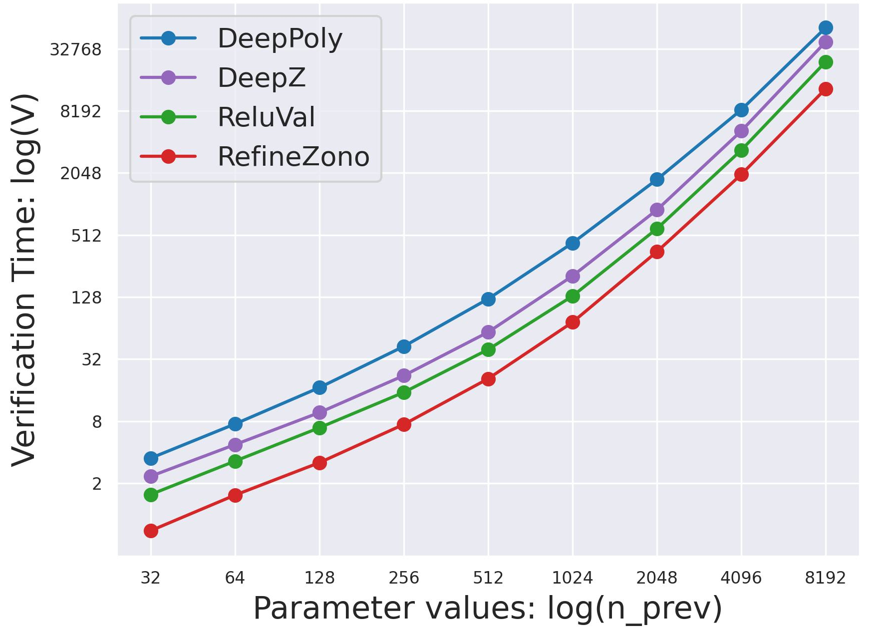
Figure 12. Verification time (in s) for correct Affine transformers.

6.3. Detecting Unsound Abstract Transformers

Using ConstraintFlow, we can identify unsound abstract transformers. We randomly introduce bugs in the existing DNN certifiers. The bugs were introduced for all DNN operations and we were able to detect unsoundness in all of them. The incorrect transformers are shown in Appendix LABEL:appendix:casestudies. For example, for the new MaxPool transformer introduced in Section LABEL:sec:newdefinitions, there can be cases where there are more than one neurons in prev that have equal values for the lower and upper bounds, i.e., $n_{1}[l]=n_{1}[u]=n_{2}[l]=n_{2}[u]$. In such a case, the output of the compare construct will be a list with more than one neuron. So, to convert the output to a polyhedral expression, one must take the average of the neurons and not the sum. Following is an incorrect implementation of the MaxPool transformer, that we can detect.

⬇

transformer DeepPoly{

MaxPool -> len(compare(prev, f)) > 0 ? (max(prev[l]), max(prev[u]), (*@\bfseries\textcolor{red}{sum}@*)(compare(prev, f)), (*@\bfseries\textcolor{red}{sum}@*)(compare(prev, f))) : (max(prev[l]), max(prev[u]),max(prev[l]), max(prev[u]));

}

The bug-finding times for the incorrect implementations of primitive operations are shown in Table 2 - column B, while those for composite operations are shown in Table 3 - column B. For Affine, we use $n_{sym}=n_{prev}=2048$, and for MaxPool, $n_{sym}=n_{prev}=10$. Similar to the verification times for correct implementations, the bug-finding times are usually less than a second. For composite operations, the bug-finding times are always less than the verification times because to disprove the query it is sufficient to find one counter-example. Note that ConstraintFlow verification procedure is not complete for traverse and solver constructs (Theorem 5.4). When solver or traverse is used, we separately check the counter-example generated by the verification procedure.

7. Related Work

DNN Certification. The recent advancements in DNN certification techniques (Albarghouthi, 2021) have led to the organization of competitions to showcase DNN certification capabilities (Brix et al., 2023), the creation of benchmark datasets (Dario Guidotti and Pulina, 2023), the introduction of a DSL for specifying certification properties (Geng et al., 2023; Shriver et al., 2021), and the development of a library for DNN certifiers (Li et al., 2023; Pham et al., 2020). However, they lack formal soundness guarantees and do not offer a systematic approach to designing new certifiers.

Symbolic Execution. Similar to ConstraintFlow DNN expansion step, previous works (Khurshid et al., 2003; Visser et al., 2004) employ lazy initialization for symbolic execution of complex data structures like lists, trees, etc. This strategy initializes object fields with symbolic values only when accessed by the program. However, unlike these works, which possess prior knowledge of the exact fields and structure of the objects, DNN certifier deals with arbitrary DAGs representing DNNs. The graph nodes (neurons) are intricate data structures linked according to an unknown graph topology. Notably, no existing solution creates a symbolic DAG with sufficient generality to represent arbitrary graph topologies.

To handle external function calls,  (Godefroid et al., 2005; Sen et al., 2005; Cadar et al., 2006) use concrete arguments creating unsoundness. To improve on this,  (Cadar et al., 2008; Chipounov et al., 2012; Bucur et al., 2011) create an abstract model to capture the semantics of the external calls. In the context of DNN certification, the external calls are restricted to optimizers such as LP, MILP, and SMT solvers. This restriction makes it possible to simulate their behavior without actually executing them on concrete inputs or creating extensive abstract models.

Invariant synthesis is done by various techniques including computing interpolants (McMillan, 2010), using widening operators and weakest preconditions for path subsumption (Jaffar et al., 2012a, b, 2009), and learning-based techniques (Si et al., 2018; D’Souza et al., 2017; Garg et al., 2014; Ezudheen et al., 2018). These methods suffer from problems like long termination times, generating insufficient invariants, etc. However, if the property to be proven is known beforehand, it can be used to guide the search for a suitable invariant. Fortunately, in ConstraintFlow, the soundness property is known beforehand. This gives an opportunity to automatically synthesize an invariant for traverse in the future.

Verification of the Certifier. The correctness of certifiers can be verified using Abstract Interpretation (Cousot et al., 2019), or by translating the verification problem to first-order logic queries and using off-the-shelf solvers (Vishwanathan et al., 2023; Lin et al., 2023). Some existing works prove the correctness of the symbolic execution w.r.t the language semantics (Keuchel et al., 2022). However, these methods establish the correctness in the scenario where symbolic execution also represents symbolic variables used in concrete executions.

8. Discussion and Future Work

We develop a new DSL ConstraintFlow that can specify state-of-the-art DNN certifiers in just a few lines of code and a verification procedure, enabling for the first time, the verification of the soundness of these DNN certifiers for arbitrary (but bounded) DAG topologies. Given the growing concerns about AI safety, we believe that ConstraintFlow can encourage the community to use DNN certification in practical applications with small effort. As a piece of evidence, the development of libraries such as TensorFlow (Abadi et al., 2016) and PyTorch (Paszke et al., 2019) has substantially propelled the widespread adoption of DNNs. Similarly, ConstraintFlow can enable faster development and deployment of DNN certifiers. Further, ConstraintFlow design allows the following future work:
Compiler Construction - The DSL and its operational semantics provide the foundation for an optimizing compiler for DNN certification algorithms.
Verification Property - In the current formulation, the verification property is the over approximation based soundness of a DNN certifier. Nevertheless, given that all the necessary formalism for verification has now been established, the property can be extended to encompass more intricate aspects, such as encoding precision of a DNN certifier w.r.t a baseline.

Appendix A ConstraintFlow DSL

¡Types¿ $t$ ::= Int — Real — Bool — Neuron — Sym — PolyExp — SymExp — Ct — $\overline{t}$

¡Binary-op¿ $\oplus$ ::= $+$ — $-$ — $*$ — $/$ — $\mathsf{and}$ — $\mathsf{or}$ — $\geq$ — $\leq$ — $==$ — <>

¡Unary-op¿ $\sim$ ::= $\mathsf{not}$

¡Neuron-metadata¿ $m$ ::= weight — bias — layer — equations

¡List-operations¿ $F_{l}$ ::= max — min

¡Solver-op¿ $\mathsf{op}$ ::= maximize — minimize

¡Function-call¿ $f_{c}$ ::= $x$

¡Transformer-call¿ $\theta_{c}$ ::= $x$

¡Direction¿ $\delta$ ::= backward — forward

¡Expression¿ $e$ ::= $c$ — $x$ — sym $e_{1}\ \oplus\ e_{2}$ — $\sim e$ $e_{1}\ ?\ e_{2}\ :\ e_{3}$ $e[m]$ — $e[x]$ $x.\texttt{\footnotesize{\color[rgb]{0.13,0.13,1}{traverse}}}(\delta,f_{c_{1}},f_{c_{2}},f_{c_{3}})\{e\}$ — $\texttt{\footnotesize{\color[rgb]{0.13,0.13,1}{solver}}}(\mathsf{op},e_{1},e_{2})$ $F_{l}(e)$ — $F_{l}(e_{1},e_{2})$ — $\texttt{\footnotesize{\color[rgb]{0.13,0.13,1}compare}}(e,f_{c})$ $\texttt{\footnotesize{\color[rgb]{0.13,0.13,1}{sum}}}(e)$ — $\texttt{\footnotesize{\color[rgb]{0.13,0.13,1}{avg}}}(e)$ — $\texttt{\footnotesize{\color[rgb]{0.13,0.13,1}{len}}}(e)$ — $e_{1}.\texttt{\footnotesize{\color[rgb]{0.13,0.13,1}{dot}}}(e_{2})$ — $e_{1}.\texttt{\footnotesize{\color[rgb]{0.13,0.13,1}concat}}(e_{2})$ $e.\texttt{\footnotesize{\color[rgb]{0.13,0.13,1}{map}}}(f_{c})$ — $e.\texttt{\footnotesize{\color[rgb]{0.13,0.13,1}{mapList}}}(f_{c})$ $f_{c}(e_{1},e_{2},\cdots)$

¡Shape-decl¿ $d$ ::= $\texttt{\footnotesize{\color[rgb]{0.13,0.13,1}{{Def shape as}}}}\ (t_{1}\ x_{1},t_{2}\ x_{2},\cdots)\{e\}$

¡Function-decl¿ $f_{d}$ ::= $\texttt{\footnotesize{\color[rgb]{0.13,0.13,1}{Func}}}\ x(t_{1}\ x_{1},t_{2}\ x_{2},\cdots)$

¡Function-definition¿ $f$ ::= $f_{d}=e$

¡DNN-operation¿ $\eta$ ::= Affine — ReLU — MaxPool — DotProduct — Sigmoid — Tanh — $\cdots$

¡Transformer-decl¿ $\theta_{d}$ ::= $\texttt{\footnotesize{\color[rgb]{0.13,0.13,1}{Transformer}}}\ x([\texttt{\footnotesize{\color[rgb]{0.13,0.13,1}{curr}}}],[\texttt{\footnotesize{\color[rgb]{0.13,0.13,1}{prev}}}])$

¡Transformer-ret¿ $\theta_{r}$ ::= $(e_{1},e_{2},\cdots)$ — $(e\ ?\ \theta_{r_{1}}:\theta_{r_{2}})$

¡Transformer¿ $\theta$ ::= $\theta_{d}=\{\eta_{1}\rightarrow\theta_{r_{1}};\eta_{2}\rightarrow\theta_{r_{2}};\cdots\}$

¡Statement¿ $s$ ::= $\texttt{\footnotesize{\color[rgb]{0.13,0.13,1}{Flow}}}(\delta,f_{c_{1}},f_{c_{2}},\theta_{c})$ — $f$ — $\theta$ — $s_{1}\ ;\ s_{2}$

¡Program¿ $\Pi$ ::= $d\ ;\ s$

Other than standard types such as $\texttt{\footnotesize{\color[rgb]{0.1,0.6,0.2}{Int}}},\texttt{\footnotesize{\color[rgb]{0.1,0.6,0.2}{Real}}},\texttt{\footnotesize{\color[rgb]{0.1,0.6,0.2}{Bool}}}$, we provide datatypes that are specific to DNN certification including $\texttt{\footnotesize{\color[rgb]{0.1,0.6,0.2}{Neuron}}},\texttt{\footnotesize{\color[rgb]{0.1,0.6,0.2}{Sym}}},\texttt{\footnotesize{\color[rgb]{0.1,0.6,0.2}{PolyExp}}},\texttt{\footnotesize{\color[rgb]{0.1,0.6,0.2}{SymExp}}},\texttt{\footnotesize{\color[rgb]{0.1,0.6,0.2}{Ct}}}$. Further, the expression of type $\overline{t}$ are lists with all the elements of type $t$.

We have the standard unary, binary, and ternary operators for expressions. The list operations include computing the sum of a list, finding the maximum or minimum element of a list, the average of a list, the length of a list, the dot product of two lists, and concatenating two lists. Further, the construct compare can be used to define the maximum of a list of neurons which takes in a user-defined function that compares two neurons. Other operations are map, mapList, traverse, solver. function call. These are explained in the main text of the paper.

The metadata of a neuron is configurable. For now, we provide weight, bias, layer number, and equations as the metadata. This can be extended to include other things that are a part of the DNN architecture. For example, we can add boolean metadata such as the ones indicating whether a neuron is a part of the input layer or a part of the output layer. The metadata equations is used to refer to a list of equations relating the neurons from the current layer to the neurons of the next layer. Each neuron in prev corresponds to one equation in $\texttt{\footnotesize{\color[rgb]{0.13,0.13,1}{curr}}}[\texttt{\footnotesize{\color[rgb]{0.13,0.13,1}{equations}}}]$. The metadata weight and bias are referred to as w and b in the main text.

Appendix B Type checking

B.1. Type checking Rules for Expressions

The general form for type-checking for expressions is $\Gamma,\tau_{s}\vdash e\ :\ t$. $\Gamma$ is a static record that stores the types of identifiers defined in the code. These identifiers include function names, transformer names, and the formal arguments of functions and transformers. $\tau_{s}$ stores the types of the shape members defined by the user. The binary operators like $+,and,\leq$ are overloaded to be also used for the new datatypes defined in ConstraintFlow. As in the rule T-comparison-1, the comparison of integers or real numbers outputs a boolean, however, in rule T-comparison-2, the comparison of two PolyExp expressions outputs a constraint of the type Ct.

$\Gamma,\tau_{s}\vdash e\ :\ t$

$$\begin{array}[]{c}\inferrule*[lab={\textsc{T-var}}]{}{\Gamma,\tau_{s}\vdash x:\Gamma(x)}\hskip 28.45274pt\inferrule*[lab={\textsc{T-noise}}]{}{\Gamma,\tau_{s}\vdash{\epsilon}:\texttt{\footnotesize{\color[rgb]{0.1,0.6,0.2}{Sym}}}}\hskip 28.45274pt\inferrule*[lab={\textsc{T-unary}}]{\Gamma,\tau_{s}\vdash e:\texttt{\footnotesize{\color[rgb]{0.1,0.6,0.2}{Bool}}}}{\Gamma,\tau_{s}\vdash\sim e:\texttt{\footnotesize{\color[rgb]{0.1,0.6,0.2}{Bool}}}}\\ \\ \inferrule*[lab={\textsc{T-comparison-1}}]{\Gamma,\tau_{s}\vdash e_{1}:t_{1}\quad\Gamma,\tau_{s}\vdash e_{2}:t_{2}\\ \\ t_{1},t_{2}\in\{\texttt{\footnotesize{\color[rgb]{0.1,0.6,0.2}{Int}}},\texttt{\footnotesize{\color[rgb]{0.1,0.6,0.2}{Real}}}\}\quad\oplus\in\{\geq,\leq,==\}}{\Gamma,\tau_{s}\vdash e_{1}\oplus e_{2}:\texttt{\footnotesize{\color[rgb]{0.1,0.6,0.2}{Bool}}}}\hskip 28.45274pt\inferrule*[lab={\textsc{T-comparison-2}}]{\Gamma,\tau_{s}\vdash e_{1}:t_{1}\quad\Gamma,\tau_{s}\vdash e_{2}:t_{2}\\ \\ t_{1}\sqcup t_{2}=t\quad\texttt{\footnotesize{\color[rgb]{0.1,0.6,0.2}{Real}}}\sqsubset t\sqsubset\top\\ \\ \oplus\in\{\geq,\leq,==\}}{\Gamma,\tau_{s}\vdash e_{1}\oplus e_{2}:\texttt{\footnotesize{\color[rgb]{0.1,0.6,0.2}{Ct}}}}\\ \\ \inferrule*[lab={\textsc{T-comparison-3}}]{\Gamma,\tau_{s}\vdash e_{1}:t_{1}\quad\Gamma,\tau_{s}\vdash e_{2}:t_{2}\\ \\ t_{1}\sqsubseteq\texttt{\footnotesize{\color[rgb]{0.1,0.6,0.2}{PolyExp}}}\\ \\ t_{2}\sqsubseteq\texttt{\footnotesize{\color[rgb]{0.1,0.6,0.2}{SymExp}}}}{\Gamma,\tau_{s}\vdash e_{1}\ \texttt{<>}\ e_{2}:\texttt{\footnotesize{\color[rgb]{0.1,0.6,0.2}{Ct}}}}\hskip 28.45274pt\inferrule*[lab={\textsc{T-binary-bool}}]{\Gamma,\tau_{s}\vdash e_{1}:t_{1}\\ \\ \Gamma,\tau_{s}\vdash e_{2}:t_{2}\\ \\ \oplus\in\{\mathsf{and},\mathsf{or}\}\quad t_{1},t_{2}\in\{\texttt{\footnotesize{\color[rgb]{0.1,0.6,0.2}{Bool}}},\texttt{\footnotesize{\color[rgb]{0.1,0.6,0.2}{Ct}}}\}}{\Gamma,\tau_{s}\vdash e_{1}\oplus e_{2}:t_{1}\sqcup t_{2}}\\ \\ \inferrule*[lab={\textsc{T-binary-arith-1}}]{\Gamma,\tau_{s}\vdash e_{1}:t_{1}\quad\Gamma,\tau_{s}\vdash e_{2}:t_{2}\\ \\ t_{1}\sqcup t_{2}\in\{\texttt{\footnotesize{\color[rgb]{0.1,0.6,0.2}{PolyExp}}},\texttt{\footnotesize{\color[rgb]{0.1,0.6,0.2}{SymExp}}}\}\\ \\ \oplus\in\{+,-\}}{\Gamma,\tau_{s}\vdash e_{1}\oplus e_{2}:t_{1}\sqcup t_{2}}\hskip 28.45274pt\inferrule*[lab={\textsc{T-binary-arith-2}}]{\Gamma,\tau_{s}\vdash e_{1}:t_{1}\quad\Gamma,\tau_{s}\vdash e_{2}:t_{2}\\ \\ t_{2}\sqsubseteq t_{1}\quad t_{2}\sqsubseteq\texttt{\footnotesize{\color[rgb]{0.1,0.6,0.2}{Real}}}\\ \\ \oplus\in\{*,/\}}{\Gamma,\tau_{s}\vdash e_{1}\oplus e_{2}:t_{1}}\\ \\ \inferrule*[lab={\textsc{T-binary-mult}}]{\Gamma,\tau_{s}\vdash e_{1}:t_{1}\quad\Gamma,\tau_{s}\vdash e_{2}:t_{2}\\ \\ t_{1}\sqcup t_{2}\in\{\texttt{\footnotesize{\color[rgb]{0.1,0.6,0.2}{PolyExp}}},\texttt{\footnotesize{\color[rgb]{0.1,0.6,0.2}{SymExp}}}\}\\ \\ t_{1}\sqsubseteq\texttt{\footnotesize{\color[rgb]{0.1,0.6,0.2}{Real}}}\ \mathsf{or}\ t_{2}\sqsubseteq\texttt{\footnotesize{\color[rgb]{0.1,0.6,0.2}{Real}}}}{\Gamma,\tau_{s}\vdash e_{1}*e_{2}:t_{1}\sqcup t_{2}}\hskip 28.45274pt\inferrule*[lab={\textsc{T-ternary}}]{\Gamma,\tau_{s}\vdash e_{1}:\texttt{\footnotesize{\color[rgb]{0.1,0.6,0.2}{Bool}}}\\ \\ \Gamma,\tau_{s}\vdash e_{2}:t_{1}\\ \\ \Gamma,\tau_{s}\vdash e_{3}:t_{2}}{\Gamma,\tau_{s}\vdash(e_{1}\ ?\ e_{2}:e_{3}):t_{1}\sqcup t_{2}}\hskip 28.45274pt\inferrule*[lab={\textsc{T-metadata-b}}]{\Gamma,\tau_{s}\vdash e:\texttt{\footnotesize{\color[rgb]{0.1,0.6,0.2}{Neuron}}}}{\Gamma,\tau_{s}\vdash e[\texttt{\footnotesize{\color[rgb]{0.13,0.13,1}{bias}}}]:\texttt{\footnotesize{\color[rgb]{0.1,0.6,0.2}{Real}}}}\\ \\ \inferrule*[lab={\textsc{T-shape}}]{\Gamma,\tau_{s}\vdash e:\texttt{\footnotesize{\color[rgb]{0.1,0.6,0.2}{Neuron}}}\\ \\ \tau_{s}(x)=t}{\Gamma,\tau_{s}\vdash e[x]:t}\hskip 28.45274pt\inferrule*[lab={\textsc{T-metadata-b2}}]{\Gamma,\tau_{s}\vdash e:\overline{\texttt{\footnotesize{\color[rgb]{0.1,0.6,0.2}{Neuron}}}}}{\Gamma,\tau_{s}\vdash e[\texttt{\footnotesize{\color[rgb]{0.13,0.13,1}{bias}}}]:\overline{\texttt{\footnotesize{\color[rgb]{0.1,0.6,0.2}{Real}}}}}\hskip 28.45274pt\inferrule*[lab={\textsc{T-metadata-shape2}}]{\Gamma,\tau_{s}\vdash e:\overline{\texttt{\footnotesize{\color[rgb]{0.1,0.6,0.2}{Neuron}}}}\\ \\ \tau_{s}(x)=t}{\Gamma,\tau_{s}\vdash e[x]:\overline{t}}\\ \\ \end{array}$$

$$\begin{array}[]{c}\inferrule*[lab={\textsc{T-min-max}}]{F_{l}\in\{\texttt{\footnotesize{\color[rgb]{0.13,0.13,1}{min}}},\texttt{\footnotesize{\color[rgb]{0.13,0.13,1}{max}}}\}\\ \\ \Gamma,\tau_{s}\vdash e:\overline{t}\quad t\sqsubseteq\texttt{\footnotesize{\color[rgb]{0.1,0.6,0.2}{Real}}}}{\Gamma,\tau_{s}\vdash F_{l}(e):t}\hskip 28.45274pt\inferrule*[lab={\textsc{T-compare}}]{\Gamma,\tau_{s}\vdash e:\overline{t}\\ \\ \Gamma(f_{c})=t\times t\rightarrow\texttt{\footnotesize{\color[rgb]{0.1,0.6,0.2}{Bool}}}}{\Gamma,\tau_{s}\vdash\texttt{\footnotesize{\color[rgb]{0.13,0.13,1}compare}}(e,f_{c}):\overline{t}}\hskip 28.45274pt\inferrule*[lab={\textsc{T-function-call}}]{\Gamma(f_{c})=(\Pi_{i}^{n}t_{i})\rightarrow t\\ \\ \forall i,\Gamma,\tau_{s}\vdash e_{i}:t_{i}}{\Gamma,\tau_{s}\vdash f_{c}(e_{1},\cdots,e_{n}):t}\\ \\ \inferrule*[lab={\textsc{T-map-poly}}]{\Gamma,\tau_{s}\vdash e:\texttt{\footnotesize{\color[rgb]{0.1,0.6,0.2}{PolyExp}}}\\ \\ \Gamma,\tau_{s}\vdash f_{c}:\texttt{\footnotesize{\color[rgb]{0.1,0.6,0.2}{Neuron}}}\times\texttt{\footnotesize{\color[rgb]{0.1,0.6,0.2}{Real}}}\rightarrow t\\ \\ t\sqsubseteq\texttt{\footnotesize{\color[rgb]{0.1,0.6,0.2}{PolyExp}}}}{\Gamma,\tau_{s}\vdash e\cdot\texttt{\footnotesize{\color[rgb]{0.13,0.13,1}{map}}}(f_{c}):\texttt{\footnotesize{\color[rgb]{0.1,0.6,0.2}{PolyExp}}}}\hskip 28.45274pt\inferrule*[lab={\textsc{T-map-sym}}]{\Gamma,\tau_{s}\vdash e:\texttt{\footnotesize{\color[rgb]{0.1,0.6,0.2}{SymExp}}}\\ \\ \Gamma,\tau_{s}\vdash f_{c}:\texttt{\footnotesize{\color[rgb]{0.1,0.6,0.2}{Sym}}}\times\texttt{\footnotesize{\color[rgb]{0.1,0.6,0.2}{Real}}}\rightarrow t\\ \\ t\sqsubseteq\texttt{\footnotesize{\color[rgb]{0.1,0.6,0.2}{SymExp}}}}{\Gamma,\tau_{s}\vdash e\cdot\texttt{\footnotesize{\color[rgb]{0.13,0.13,1}{map}}}(f_{c}):\texttt{\footnotesize{\color[rgb]{0.1,0.6,0.2}{PolyExp}}}}\\ \\ \inferrule*[lab={\textsc{T-map-list}}]{\Gamma,\tau_{s}\vdash e:\overline{t}\\ \\ \Gamma,\tau_{s}\vdash f_{c}:t\rightarrow t^{\prime}\\ \\ t\sqsubseteq\texttt{\footnotesize{\color[rgb]{0.1,0.6,0.2}{PolyExp}}}\mathsf{or}t\sqsubseteq\texttt{\footnotesize{\color[rgb]{0.1,0.6,0.2}{SymExp}}}\\ \\ t\in\{\texttt{\footnotesize{\color[rgb]{0.1,0.6,0.2}{Neuron}}},\texttt{\footnotesize{\color[rgb]{0.1,0.6,0.2}{PolyExp}}}\}\implies t^{\prime}=\texttt{\footnotesize{\color[rgb]{0.1,0.6,0.2}{PolyExp}}}\\ \\ t\in\{\texttt{\footnotesize{\color[rgb]{0.1,0.6,0.2}{Sym}}},\texttt{\footnotesize{\color[rgb]{0.1,0.6,0.2}{SymExp}}}\}\implies t^{\prime}=\texttt{\footnotesize{\color[rgb]{0.1,0.6,0.2}{SymExp}}}\\ \\ \text{otherwise }t^{\prime}=t}{\Gamma,\tau_{s}\vdash e\cdot\texttt{\footnotesize{\color[rgb]{0.13,0.13,1}{map}}}(f_{c}):t^{\prime}}\hskip 28.45274pt\inferrule*[lab={\textsc{T-solver}}]{\Gamma,\tau_{s}\vdash e_{1}:\texttt{\footnotesize{\color[rgb]{0.1,0.6,0.2}{PolyExp}}}\\ \\ \Gamma,\tau_{s}\vdash e_{2}:\texttt{\footnotesize{\color[rgb]{0.1,0.6,0.2}{Ct}}}}{\Gamma,\tau_{s}\vdash\texttt{\footnotesize{\color[rgb]{0.13,0.13,1}{solver}}}(\mathsf{op},e_{1},e_{2}):\texttt{\footnotesize{\color[rgb]{0.1,0.6,0.2}{Real}}}}\\ \\ \inferrule*[lab={\textsc{T-traverse}}]{\Gamma,\tau_{s}\vdash e_{1}:\texttt{\footnotesize{\color[rgb]{0.1,0.6,0.2}{PolyExp}}}\quad\Gamma,\tau_{s}\vdash e_{2}:\texttt{\footnotesize{\color[rgb]{0.1,0.6,0.2}{Ct}}}\\ \\ \Gamma,\tau_{s}\vdash f_{c_{1}}:\texttt{\footnotesize{\color[rgb]{0.1,0.6,0.2}{Neuron}}}\rightarrow t^{\prime}\quad\Gamma,\tau_{s}\vdash f_{c_{2}}:\texttt{\footnotesize{\color[rgb]{0.1,0.6,0.2}{Neuron}}}\rightarrow\texttt{\footnotesize{\color[rgb]{0.1,0.6,0.2}{Bool}}}\\ \\ \Gamma,\tau_{s}\vdash f_{c_{3}}:\texttt{\footnotesize{\color[rgb]{0.1,0.6,0.2}{Neuron}}}\times\texttt{\footnotesize{\color[rgb]{0.1,0.6,0.2}{Real}}}\rightarrow t^{\prime\prime}\\ \\ \bot\sqsubset t^{\prime}\sqsubseteq\texttt{\footnotesize{\color[rgb]{0.1,0.6,0.2}{Real}}}\quad\bot\sqsubset t^{\prime\prime}\sqsubseteq\texttt{\footnotesize{\color[rgb]{0.1,0.6,0.2}{PolyExp}}}}{\Gamma,\tau_{s}\vdash e_{1}.\texttt{\footnotesize{\color[rgb]{0.13,0.13,1}{traverse}}}(\delta,f_{c_{1}},f_{c_{2}},f_{c_{3}})\{e_{2}\}:\texttt{\footnotesize{\color[rgb]{0.1,0.6,0.2}{PolyExp}}}}\end{array}$$

B.2. Type checking Rules for Statements

The rules for type-checking statements update either $\tau_{s}$ or $\Gamma$. For function definition statements where the arguments are of the type $t_{1},\cdots,t_{n}$ and the return expression is of type $t$, the type of the function is $(\Pi_{i}^{n}t_{i})\rightarrow t$. $\Gamma$ is updated to map the function name to this type. For transformer definition statements, if they take in the inputs curr and prev, which are optional, the inputs are of type Neuron and $\overline{\texttt{\footnotesize{\color[rgb]{0.1,0.6,0.2}{Neuron}}}}$. The output tuples returned by transformers are the join of the output tuples returned by the return expression of each operation. The type of each transformer is also stored in $\Gamma$. The type of the shape declaration statement is $[t_{1},\cdots,t_{n}]$, where $t_{i}$ is the type of the $i$th declared shape member.

$\Gamma,\tau_{s}\vdash s\ :\ \Gamma^{\prime}$

$$\begin{array}[]{c}\inferrule*[lab={\footnotesize{\textsc{T-func}}}]{\Gamma^{\prime}=\Gamma[x_{1}\mapsto t_{1},\cdots x_{n}\mapsto t_{n}]\\ \\ x\not\in\Gamma\quad\Gamma^{\prime},\tau_{s}\vdash e:t\quad\bot\sqsubset t\sqsubset\top}{\Gamma,\tau_{s}\vdash\texttt{\footnotesize{\color[rgb]{0.13,0.13,1}{Func}}}\ x(t_{1}\ x_{1},\cdots t_{n}\ x_{n})=e:\Gamma[x\mapsto(\Pi_{i}^{n}t_{i})\rightarrow t]}\hskip 28.45274pt\inferrule*[lab=\textsc{T-transformer-call}]{\Gamma(\theta_{c})=\tau}{\Gamma,\tau_{s}\vdash\theta_{c}:\tau}\\ \\ \inferrule*[lab={\textsc{T-transformer-ret-1}}]{\forall i\in[n],\Gamma,\tau_{s}\vdash e_{i}:t_{i}\quad t_{i}\sqsubseteq\tau_{s}(i)}{\Gamma,\tau_{s}\vdash(e_{1},\cdots,e_{n}):(t_{1},\cdots,t_{n})}\hskip 28.45274pt\inferrule*[lab={\textsc{T-transformer-ret-2}}]{\Gamma,\tau_{s}\vdash e:\texttt{\footnotesize{\color[rgb]{0.1,0.6,0.2}{Bool}}}\\ \\ \Gamma,\tau_{s}\vdash\theta_{r_{1}}:(t^{\prime}_{1},\cdots,t^{\prime}_{n})\\ \\ \Gamma,\tau_{s}\vdash\theta_{r_{2}}:(t^{\prime\prime}_{1},\cdots,t^{\prime\prime}_{n})\\ \\ \forall i\in[n],t_{i}=t^{\prime}_{i}\sqcup t^{\prime\prime}_{i}\sqsubset\top}{\Gamma,\tau_{s}\vdash\texttt{\footnotesize{\color[rgb]{0.13,0.13,1}{if}}}(e,\theta_{r_{1}},\theta_{r_{2}}):(t_{1},\cdots,t_{n})}\\ \\ \inferrule*[lab={\textsc{T-transformer}}]{\Gamma^{\prime}=\Gamma[\texttt{\footnotesize{\color[rgb]{0.13,0.13,1}{curr}}}\mapsto\texttt{\footnotesize{\color[rgb]{0.1,0.6,0.2}{Neuron}}})][\texttt{\footnotesize{\color[rgb]{0.13,0.13,1}{prev}}}\mapsto\overline{\texttt{\footnotesize{\color[rgb]{0.1,0.6,0.2}{Neuron}}}}]\\ \\ \forall i\in[m],\Gamma^{\prime},\tau_{s}\vdash\theta_{r_{i}}:(t^{1}_{i},\cdots,t^{n}_{i})\\ \\ x\not\in\Gamma\quad\forall j\in[n],t^{j}=\sqcup_{i\in[m]}(t^{j}_{i})\quad t^{j}\sqsubseteq\tau^{j}_{s}}{\Gamma,\tau_{s}\vdash\texttt{\footnotesize{\color[rgb]{0.13,0.13,1}{Transformer}}}\ x(\texttt{\footnotesize{\color[rgb]{0.13,0.13,1}{curr}}},\texttt{\footnotesize{\color[rgb]{0.13,0.13,1}{prev}}})=\{\eta_{1}:\theta_{r_{1}},\cdots\}:\Gamma[x\mapsto(\texttt{\footnotesize{\color[rgb]{0.1,0.6,0.2}{Neuron}}}\times\overline{\texttt{\footnotesize{\color[rgb]{0.1,0.6,0.2}{Neuron}}}})\rightarrow(t^{1},\cdots)]}\\ \\ \inferrule*[lab={\textsc{T-flow}}]{\Gamma,\tau_{s}\vdash f_{c_{1}}:\texttt{\footnotesize{\color[rgb]{0.1,0.6,0.2}{Neuron}}}\rightarrow t^{\prime}\\ \\ \Gamma,\tau_{s}\vdash f_{c_{2}}:\texttt{\footnotesize{\color[rgb]{0.1,0.6,0.2}{Neuron}}}\rightarrow\texttt{\footnotesize{\color[rgb]{0.1,0.6,0.2}{Bool}}}\\ \\ \theta_{c}\in\Gamma\quad t^{\prime}\sqsubseteq\texttt{\footnotesize{\color[rgb]{0.1,0.6,0.2}{Real}}}}{\Gamma,\tau_{s}\vdash\texttt{\footnotesize{\color[rgb]{0.13,0.13,1}{Flow}}}(\delta,f_{c_{1}},f_{c_{2}},\theta_{c}):\Gamma}\hskip 28.45274pt\inferrule*[lab={\textsc{T-seq}}]{\Gamma,\tau_{s}\vdash s_{1}:\Gamma^{\prime}\\ \\ \Gamma^{\prime},\tau_{s}\vdash s_{2}:\Gamma^{\prime\prime}}{\Gamma,\tau_{s}\vdash s_{1}\ ;\ s_{2}:\Gamma^{\prime\prime}}\end{array}$$

$\cdot\ \vdash d\ :\ \tau_{s}$

$$\begin{array}[]{c}\inferrule*[lab={\textsc{T-shape}}]{\tau_{s}=[x_{1}\mapsto t_{1},\cdots x_{n}\mapsto t_{n}]\\ \\ \forall i\in[n],\bot\sqsubset t_{i}\sqsubset\top}{\cdot\ \vdash\texttt{\footnotesize{\color[rgb]{0.13,0.13,1}{{Def shape as}}}}\ (t_{1}\ x_{1},\cdots,t_{n}\ x_{n}):\tau_{s}}\end{array}$$

$\cdot\ \vdash\Pi\ :\ \Gamma,\tau_{s}$

$$\begin{array}[]{c}\inferrule*[lab={\textsc{T-program}}]{\cdot\vdash d:\tau_{s}\quad\cdot,\tau_{s}\vdash s:\Gamma}{\cdot\ \vdash d\ ;\ s\ :\ \Gamma,\tau_{s}}\end{array}$$

Appendix C Concrete Values in ConstraintFlow

C.1. Definition

¡constant¿ $c$ ::= $1$ — $2$ — $3$ — $\cdots$ — $\mathsf{true}$ — $\mathsf{false}$

¡PolyVal¿ $\nu_{p}$ ::= $c$ — $c*n$ — $\nu_{p}^{\prime}+\nu_{p}^{\prime\prime}$

¡SymVal¿ $\nu_{s}$ ::= $c$ — $c*{\epsilon}$ — $\nu_{s}^{\prime}+\nu_{s}^{\prime\prime}$

¡CtVal¿ $\nu_{c}$ ::= $\nu_{p}==\nu_{p}$ — $\nu_{p}\ \texttt{<>}\ \nu_{s}$

¡Base-val¿ $\nu_{b}$ ::= $c$ — $\nu_{p}$ — $\nu_{s}$ — $\nu_{c}$

¡List-val¿ $\nu_{l}$ ::= $[\nu_{b_{1}},\nu_{b_{2}},\cdots]$

¡Val¿ $\nu$ ::= $\nu_{b}$ — $\nu_{l}$

These are the possible values a concrete expression can evaluate using the operational semantics. The value can be a constant, integer, real number, or boolean. The value can also be a neuron or symbolic variable, or an affine combination of either, which would result in a polyhedral expression or symbolic expression. Since we allow solvers in the operational semantics, constraints, stating that two polyhedral values are equal or a polyhedral value is embedded in a symbolic expression, are also values. Lists of values are also valid values.

C.2. Operations on Concrete Values

$\texttt{\footnotesize{\color[rgb]{0.13,0.13,1}{max}}}(\nu_{l})$

$$\begin{array}[]{c}\inferrule*[lab=\textsc{V-max-emp}]{\nu_{l}=[]}{\texttt{\footnotesize{\color[rgb]{0.13,0.13,1}{max}}}(\nu_{l})=0}\hskip 28.45274pt\inferrule*[lab=\textsc{V-max-non-emp}]{\nu_{l}=[\nu_{b}]}{\texttt{\footnotesize{\color[rgb]{0.13,0.13,1}{max}}}(\nu_{l})=\nu_{b}}\hskip 28.45274pt\inferrule*[lab=\textsc{V-max-non-emp-r}]{\nu_{l}=\nu_{b}^{\prime\prime}::\nu_{l}^{\prime}\quad\nu_{b}^{\prime}=\texttt{\footnotesize{\color[rgb]{0.13,0.13,1}{max}}}(\nu_{l}^{\prime})\\ \\ \nu_{b}^{\prime\prime}\geq\nu_{b}^{\prime}\implies\nu_{b}=\nu_{b}^{\prime\prime}\\ \\ \nu_{b}^{\prime\prime}<\nu_{b}^{\prime}\implies\nu_{b}=\nu_{b}^{\prime}}{\texttt{\footnotesize{\color[rgb]{0.13,0.13,1}{max}}}(\nu_{l})=\nu_{b}}\end{array}$$

These are the rules for computing the maximum value of a list. The lists on which this operation is supported can only be of types $\overline{\texttt{\footnotesize{\color[rgb]{0.1,0.6,0.2}{Int}}}}$ and $\overline{\texttt{\footnotesize{\color[rgb]{0.1,0.6,0.2}{Real}}}}$ so the operations $\geq$ and $<$ are defined. These rules recursively compute the maximum element of the list by comparing each element to the maximum of the remaining elements in the list.

$\texttt{\footnotesize{\color[rgb]{0.13,0.13,1}{min}}}(\nu_{l})$

$$\begin{array}[]{c}\inferrule*[lab=\textsc{V-min-emp}]{\nu_{l}=[]}{\texttt{\footnotesize{\color[rgb]{0.13,0.13,1}{min}}}(\nu_{l})=0}\hskip 28.45274pt\inferrule*[lab=\textsc{V-min-non-emp}]{\nu_{l}=[\nu_{b}]}{\texttt{\footnotesize{\color[rgb]{0.13,0.13,1}{min}}}(\nu_{l})=\nu_{b}}\hskip 28.45274pt\inferrule*[lab=\textsc{V-min-non-emp-r}]{\nu_{l}=\nu_{b}^{\prime\prime}::\nu_{l}^{\prime}\quad\nu_{b}^{\prime}=\texttt{\footnotesize{\color[rgb]{0.13,0.13,1}{min}}}(\nu_{l}^{\prime})\\ \\ \nu_{b}^{\prime\prime}\leq\nu_{b}^{\prime}\implies\nu_{b}=\nu_{b}^{\prime\prime}\\ \\ \nu_{b}^{\prime\prime}>\nu_{b}^{\prime}\implies\nu_{b}=\nu_{b}^{\prime}}{\texttt{\footnotesize{\color[rgb]{0.13,0.13,1}{min}}}(\nu_{l})=\nu_{b}}\end{array}$$

These rules are similar to the above rules, except they compute the minimum element of a list, instead of the maximum one.

$\texttt{\footnotesize{\color[rgb]{0.13,0.13,1}compare}}(\nu_{l},f_{c},F,\rho,\mathcal{D}_{C})$

$$\begin{array}[]{c}\inferrule*[lab=\textsc{Compare}]{\nu_{l}=[\nu_{b_{1}},\cdots\nu_{b_{n}}]\quad F[f_{c}]=(x_{1},x_{2}),e\\ \\ \forall i\in[n],\rho_{i}=\rho[x_{1}\mapsto\nu_{b},x_{2}\mapsto\nu_{b_{i}}]\\ \\ \langle e,F,\rho_{i},\mathcal{D}_{C}\rangle\Downarrow\nu^{\prime}_{b_{i}}\quad\nu_{b}^{\prime}=\bigwedge^{n}_{i=1}\nu^{\prime}_{b_{i}}\\ \\ \nu_{b}^{\prime}=\mathsf{true}\implies\nu_{l}^{\prime\prime}=\nu_{b}::\nu_{l}^{\prime}\quad\nu_{b}^{\prime}=\mathsf{false}\implies\nu_{l}^{\prime\prime}=\nu_{l}^{\prime}}{\texttt{\footnotesize{\color[rgb]{0.13,0.13,1}compare}}(\nu_{b},\nu_{l},\nu_{l}^{\prime},f_{c},F,\rho,\mathcal{D}_{C})=\nu_{l}^{\prime\prime}}\hskip 14.22636pt\inferrule*[lab=\textsc{Compare-non-emp}]{\nu_{l_{1}}=\nu_{b}::\nu_{l}\\ \\ \ \nu_{l_{4}}=\texttt{\footnotesize{\color[rgb]{0.13,0.13,1}compare}}(\nu_{b},\nu_{l_{2}},\nu_{l_{3}},F,\rho,\mathcal{D}_{C})\\ \\ \nu_{l_{5}}=\texttt{\footnotesize{\color[rgb]{0.13,0.13,1}compare}}(\nu_{l},\nu_{l_{2}},\nu_{l_{4}},f_{c},F,\rho,\mathcal{D}_{C})}{\texttt{\footnotesize{\color[rgb]{0.13,0.13,1}compare}}(\nu_{l_{1}},\nu_{l_{2}},\nu_{l_{3}},f_{c},F,\rho,\mathcal{D}_{C})=\nu_{l_{5}}}\\ \\ \inferrule*[lab=\textsc{Compare-emp}]{\nu_{l_{1}}=[]}{\texttt{\footnotesize{\color[rgb]{0.13,0.13,1}compare}}(\nu_{l_{1}},\nu_{l_{2}},\nu_{l_{3}},f_{c},F,\rho,\mathcal{D}_{C})=\nu_{l_{3}}}\hskip 28.45274pt\inferrule*[lab=\textsc{V-compare-emp}]{\nu_{l}=[]}{\texttt{\footnotesize{\color[rgb]{0.13,0.13,1}compare}}(\nu_{l},f_{c},F,\rho,\mathcal{D}_{C})=\nu_{l}}\\ \\ \end{array}$$

$$\begin{array}[]{c}\inferrule*[lab=\textsc{V-compare-non-emp}]{\nu_{l}=[\nu_{b}]}{\texttt{\footnotesize{\color[rgb]{0.13,0.13,1}compare}}(\nu_{l},f_{c},F,\rho,\mathcal{D}_{C})=\nu_{l}}\hskip 28.45274pt\inferrule*[lab=\textsc{V-compare-non-emp-r}]{\nu_{l}=[\nu_{b_{1}},\cdots\nu_{b_{n}}]\\ \\ \nu_{l}^{\prime}=\texttt{\footnotesize{\color[rgb]{0.13,0.13,1}compare}}(\nu_{l},\nu_{l},[],f_{c},F,\rho,\mathcal{D}_{C})}{\texttt{\footnotesize{\color[rgb]{0.13,0.13,1}compare}}(\nu_{l},f_{c},F,\rho,\mathcal{D}_{C})=\nu_{l}^{\prime}}\end{array}$$

These rules define the compare operation. This operation takes as input a list and a function. The function has to take in two arguments, which will be members of the list, and return true if the first argument is greater than the second argument. The compare operation returns a list of all of the elements in the input list that are greater than all other elements. Depending on the function provided, this list could be empty, have one element, or more than one element. The rules Compare, Compare-non-emp, and Compare-emp compute the list of maximum elements while keeping track of an accumulated list of maximums. The rules V-compare-emp, and V-compare-non-emp state that the maximum of a list with 0 or 1 element is that same list.

C.3. Value typing

$$\begin{array}[]{c}\inferrule*[lab={\textsc{V-int}}]{}{\vdash c_{i}:\texttt{\footnotesize{\color[rgb]{0.1,0.6,0.2}{Int}}}}\hskip 28.45274pt\inferrule*[lab={\textsc{V-real}}]{}{\vdash c_{r}:\texttt{\footnotesize{\color[rgb]{0.1,0.6,0.2}{Real}}}}\hskip 28.45274pt\inferrule*[lab={\textsc{V-true}}]{}{\vdash\mathsf{true}:\texttt{\footnotesize{\color[rgb]{0.1,0.6,0.2}{Bool}}}}\hskip 28.45274pt\inferrule*[lab={\textsc{V-false}}]{}{\vdash\mathsf{false}:\texttt{\footnotesize{\color[rgb]{0.1,0.6,0.2}{Bool}}}}\\ \\ \inferrule*[lab={\textsc{V-sym}}]{}{\vdash{\epsilon}:\texttt{\footnotesize{\color[rgb]{0.1,0.6,0.2}{Sym}}}}\hskip 28.45274pt\inferrule*[lab={\textsc{V-neuron}}]{}{\vdash n:\texttt{\footnotesize{\color[rgb]{0.1,0.6,0.2}{Neuron}}}}\hskip 28.45274pt\inferrule*[lab={\textsc{V-polyexp}}]{}{\vdash c+\sum c*n:\texttt{\footnotesize{\color[rgb]{0.1,0.6,0.2}{PolyExp}}}}\hskip 28.45274pt\inferrule*[lab={\textsc{V-symexp}}]{}{\vdash c+\sum c*{\epsilon}:\texttt{\footnotesize{\color[rgb]{0.1,0.6,0.2}{SymExp}}}}\\ \\ \inferrule*[lab={\textsc{V-ct-1}}]{\vdash\nu_{1}:t_{1}\quad\vdash\nu_{2}:t_{2}\\ \\ t_{1}\sqcup t_{2}\in\{\texttt{\footnotesize{\color[rgb]{0.1,0.6,0.2}{PolyExp}}},\texttt{\footnotesize{\color[rgb]{0.1,0.6,0.2}{SymExp}}}\}\\ \\ \oplus\in\{\geq,\leq,==\}}{\vdash\nu_{1}\oplus\nu_{2}:\texttt{\footnotesize{\color[rgb]{0.1,0.6,0.2}{Ct}}}}\hskip 28.45274pt\inferrule*[lab={\textsc{V-ct-2}}]{\vdash\nu_{1}:\texttt{\footnotesize{\color[rgb]{0.1,0.6,0.2}{PolyExp}}}\quad\vdash\nu_{2}:\texttt{\footnotesize{\color[rgb]{0.1,0.6,0.2}{SymExp}}}}{\vdash\nu_{1}\texttt{<>}\nu_{2}:\texttt{\footnotesize{\color[rgb]{0.1,0.6,0.2}{Ct}}}}\hskip 28.45274pt\inferrule*[lab={\textsc{V-list}}]{\vdash\nu_{i}:t_{i}\quad t=\bigsqcup^{n}_{i=1}t_{i}}{\vdash[\nu_{1},\cdots\nu_{n}]:\overline{t}}\end{array}$$

These are the types of possible values in concrete execution. Integers, real numbers, and boolean values have the standard types. Neurons, polyhedral expressions, symbolic variables, and symbolic expressions have the types Neuron, PolyExp, Sym and SymExp respectively. Constraints also use the specialized type, Ct. A list of values, which have the type $t$, has the type $\overline{t}$

Appendix D Operational Semantics of Constraint Flow

D.1. Operational semantics for expressions

The general form for operational semantics for expressions is $\langle e,F,\rho,\mathcal{D}_{C}\rangle\Downarrow\nu$. $F$ is a static record that stores the function names, their formal arguments, and the return expression from the function definitions. $\rho$ maps variables to values. $\mathcal{D}_{C}$ represents the concrete DNN. It maps each neuron’s shape members and metadata to the corresponding concrete value, which comes from the input to the DNN certifier algorithm. The rules Op-shape and Op-metadata evaluate the expression before the shape member or metadata access, and then for the neuron, or each neuron in a list, output the value of the specified shape member or metadata from $\mathcal{D}_{C}$. The rule Op-compare refers to Compare, Compare-non-emp, and Compare-emp defined above. The Traverse rule maintains an active set, that starts from the neurons in its input polyhedral expression. Then, it filters out the elements of the active set for which the stopping condition, $f_{c_{2}}$, evaluates to true, using the rule Filter. After this, it applies the replacement function, $f_{c_{3}}$, to the neurons, and their corresponding coefficient, in the active set with the highest priority (found using the rule Priority). For each neuron to which the replacement function is applied, this neuron is removed from the active set and its neighbors (found using the rule Neighbour). The neighbors are defined as the nodes with outgoing edges to a neuron when traversing in the backward direction and the neurons with incoming edges from a neuron when traversing in the forward direction. All of these steps are repeated while the active set is not empty.

$\langle e,F,\rho,\mathcal{D}_{C}\rangle\Downarrow\nu$

$$\begin{array}[]{c}\inferrule*[lab=\textsc{Op-const}]{}{\langle c,F,\rho,\mathcal{D}_{C}\rangle\Downarrow c}\hskip 28.45274pt\inferrule*[lab=\textsc{Op-var}]{}{\langle x,F,\rho,\mathcal{D}_{C}\rangle\Downarrow\rho(x)}\hskip 28.45274pt\inferrule*[lab=\textsc{Op-sym}]{}{\langle{\epsilon},F,\rho,\mathcal{D}_{C}\rangle\Downarrow{\epsilon}_{new}}\\ \\ \inferrule*[lab=\textsc{Op-unary}]{\langle e,F,\rho,\mathcal{D}_{C}\rangle\Downarrow\nu}{\langle\sim e,F,\rho,\mathcal{D}_{C}\rangle\Downarrow\ \sim\nu}\hskip 28.45274pt\inferrule*[lab=\textsc{Op-binary}]{\langle e_{1},F,\rho,\mathcal{D}_{C}\rangle\Downarrow\nu_{1}\\ \\ \langle e_{2},F,\rho,\mathcal{D}_{C}\rangle\Downarrow\nu_{2}}{\langle e_{1}\oplus e_{2},F,\rho,\mathcal{D}_{C}\rangle\Downarrow\nu_{1}\oplus\nu_{2}}\hskip 28.45274pt\inferrule*[lab=\textsc{Op-ternary}]{\langle e_{1},F,\rho,\mathcal{D}_{C}\rangle\Downarrow\nu_{b_{1}}\\ \\ \langle e_{2},F,\rho,\mathcal{D}_{C}\rangle\Downarrow\nu_{2}\\ \\ \langle e_{3},F,\rho,\mathcal{D}_{C}\rangle\Downarrow\nu_{3}\\ \\ \nu_{b_{1}}=\mathsf{true}\implies\nu=\nu_{2}\\ \\ \nu_{b_{1}}=\mathsf{false}\implies\nu=\nu_{3}}{\langle(e_{1}?e_{2}:e_{3}),F,\rho,\mathcal{D}_{C}\rangle\Downarrow\nu}\\ \\ \inferrule*[lab=\textsc{Op-metadata}]{\langle e,F,\rho,\mathcal{D}_{C}\rangle\Downarrow n\\ \\ \nu=\mathcal{D}_{C}[n[m]]}{\langle e[m],F,\rho,\mathcal{D}_{C}\rangle\Downarrow\nu}\hskip 28.45274pt\inferrule*[lab=\textsc{Op-shape}]{\langle e.F,\rho,\mathcal{D}_{C}\rangle\Downarrow n\\ \\ \nu=\mathcal{D}_{C}[n[x]]}{\langle e[x],F,\rho,\mathcal{D}_{C}\rangle\Downarrow\nu}\\ \\ \inferrule*[lab=\textsc{Op-max}]{\langle e,F,\rho,\mathcal{D}_{C}\rangle\Downarrow\nu^{\prime}}{\langle\texttt{\footnotesize{\color[rgb]{0.13,0.13,1}{max}}}(e),F,\rho,\mathcal{D}_{C}\rangle\Downarrow\max(\nu^{\prime})}\hskip 28.45274pt\inferrule*[lab=\textsc{Op-compare}]{\langle e,F,\rho,\mathcal{D}_{C}\rangle\Downarrow\nu^{\prime}\\ \\ \nu=\texttt{\footnotesize{\color[rgb]{0.13,0.13,1}compare}}(\nu^{\prime},f_{c},F,\rho,\mathcal{D}_{C})}{\langle\texttt{\footnotesize{\color[rgb]{0.13,0.13,1}compare}}(e,f_{c}),F,\rho,\mathcal{D}_{C}\rangle\Downarrow\nu}\\ \\ \\ \\ \end{array}$$

$$\begin{array}[]{c}\inferrule*[lab=\textsc{Op-func-call}]{\forall i\in[n],\ \langle e,F,\rho,\mathcal{D}_{C}\rangle\Downarrow\nu_{i}\\ \\ F(f_{c})=(x_{1},\cdots,x_{n}),e\\ \\ \rho^{\prime}=\rho[x_{1}\mapsto\nu_{1},\cdots x_{n}\mapsto\nu_{n}]\\ \\ \langle e,F,\rho^{\prime},\mathcal{D}_{C}\rangle\Downarrow\nu}{\langle f_{c}(e_{1},\cdots,e_{n}),F,\rho,\mathcal{D}_{C}\rangle\Downarrow\nu}\hskip 28.45274pt\inferrule*[lab=\textsc{Op-map}]{\langle e,F,\rho,\mathcal{D}_{C}\rangle\Downarrow\nu_{b}^{\prime}\quad\nu_{b}^{\prime}=c_{0}+\sum_{i=0}^{i=l}c_{i}\cdot v_{i}\\ \\ \forall i\in[l],\ \langle f_{c}(v_{i},c_{i}),F,\rho,\mathcal{D}_{C}\rangle\Downarrow\nu_{i}\quad\nu_{b}=c_{0}+\sum_{i=0}^{i=l}\nu_{i}}{\langle e.\texttt{\footnotesize{\color[rgb]{0.13,0.13,1}{map}}}(f_{c}),F,\rho,\mathcal{D}_{C}\rangle\Downarrow\nu_{b}}\\ \\ \inferrule*[lab=\textsc{Filter}]{\mathsf{V}^{\prime}=\{v^{\prime}\ |\ (v^{\prime}\in\mathsf{V})\wedge(\langle f_{c}(v^{\prime}),F,\rho,\mathcal{D}_{C}\rangle\Downarrow\mathsf{false})\}}{\mathsf{Ft}(\mathsf{V},f_{c},F,\rho,\mathcal{D}_{C})=\mathsf{V}^{\prime}}\\ \\ \inferrule*[lab=\textsc{Priority}]{\forall v_{i}\in\mathsf{V},\langle f_{c}(v_{i}),F,\rho,\mathcal{D}_{C}\rangle\Downarrow\nu_{i}\\ \\ m=\max_{i}(\nu_{i})\\ \\ \mathsf{V}^{\prime}=\{v^{\prime}\ |\ (v^{\prime}\in\mathsf{V})\wedge(\langle f_{c}(v^{\prime}),F,\rho,\mathcal{D}_{C}\rangle\Downarrow m\}}{\mathsf{P}(\mathsf{V},f_{c},F,\rho,\mathcal{D}_{C})=\mathsf{V}^{\prime}}\\ \\ \inferrule*[lab=\textsc{Neighbour}]{\delta=\texttt{\footnotesize{\color[rgb]{0.13,0.13,1}{forward}}}\implies\mathsf{V}^{\prime}=\{v^{\prime}\ |\ (v,v^{\prime}\in E)\}\\ \\ \delta=\texttt{\footnotesize{\color[rgb]{0.13,0.13,1}{backward}}}\implies\mathsf{V}^{\prime}=\{v^{\prime}\ |\ (v^{\prime},v\in E)\}}{\mathsf{N}(\mathsf{V},\delta)=\mathsf{V}^{\prime}}\\ \\ \inferrule*[lab=\textsc{Vertices}]{\nu=c_{0}+c_{1}\cdot v_{1}+\cdots+c_{l}\cdot v_{l}}{\mathsf{neurons}(\nu)=\{v_{1},\cdots,v_{l}\}}\hskip 28.45274pt\inferrule*[lab=\textsc{Vertices-2}]{\nu=c_{0}+c_{1}\cdot v_{1}+\cdots+c_{l}\cdot v_{l}}{\nu_{\mathsf{V}}=\sum_{v_{j}\in\mathsf{V}}c_{j}\cdot v_{j}}\\ \\ \inferrule*[lab=\textsc{Op-traverse-1}]{}{\langle\nu.\texttt{\footnotesize{\color[rgb]{0.13,0.13,1}{traverse}}}(\delta^{\prime},f_{c_{1}},f_{c_{2}},f_{c_{3}}),F,\rho,\mathcal{D}_{C},\{\}\rangle\Downarrow\nu}\\ \\ \inferrule*[lab=\textsc{Op-traverse-2}]{\mathsf{V}^{\prime}=\mathsf{P}(\mathsf{V},f_{c_{1}},F,\rho,\mathcal{D}_{C})\quad\nu=c+\nu_{\mathsf{V}^{\prime}}+\nu_{\overline{\mathsf{V}^{\prime}}}\\ \\ \langle\nu_{\mathsf{V}^{\prime}}.\texttt{\footnotesize{\color[rgb]{0.13,0.13,1}{map}}}(f_{c_{3}}),F,\rho,\mathcal{D}_{C}\rangle\Downarrow\nu^{\prime}\\ \\ \nu^{\prime\prime}=c+\nu^{\prime}+\nu_{\overline{\mathsf{V}^{\prime}}}\\ \\ \mathsf{V}^{\prime\prime}=\mathsf{Ft}((\mathsf{V}\setminus\mathsf{V}^{\prime})\cup\mathsf{N}(\mathsf{V}^{\prime},\delta),f_{c_{2}},F,\rho,\mathcal{D}_{C})\\ \\ \langle\nu^{\prime\prime}.\texttt{\footnotesize{\color[rgb]{0.13,0.13,1}{traverse}}},F,\rho,\mathcal{D}_{C},\mathsf{V}^{\prime\prime}\rangle\Downarrow\nu^{\prime\prime\prime}}{\langle\nu.\texttt{\footnotesize{\color[rgb]{0.13,0.13,1}{traverse}}}(\delta,f_{c_{1}},f_{c_{2}},f_{c_{3}}),F,\rho,\mathcal{D}_{C},\mathsf{V}\rangle\Downarrow\nu^{\prime\prime\prime}}\\ \\ \inferrule*[lab=\textsc{Op-traverse}]{\langle e,F,\rho,\mathcal{D}_{C}\rangle\Downarrow\nu\quad\mathsf{V}=\mathsf{Ft}(\mathsf{neurons}(\nu),f_{c_{2}},F,\rho,\mathcal{D}_{C})\\ \\ \langle\nu.\texttt{\footnotesize{\color[rgb]{0.13,0.13,1}{traverse}}}(\delta,f_{c_{1}},f_{c_{2}},f_{c_{3}}),F,\rho,\mathcal{D}_{C},\mathsf{V}\rangle\Downarrow\nu^{\prime}}{\langle e_{1}.\texttt{\footnotesize{\color[rgb]{0.13,0.13,1}{traverse}}}(\delta,f_{c_{1}},f_{c_{2}},f_{c_{3}})\{\_\},F,\rho,\mathcal{D}_{C}\rangle\Downarrow\nu^{\prime}}\end{array}$$

D.2. Operation semantics for statements

In operational semantics for statements, function definition statements modify $F$ by adding the function name, arguments, and return expression. Transformer definitions similarly modify $\Theta$ by adding the return tuples for each operation to $\Theta$, which is mapped to by the transformer name. The rules for the flow statement specify that if the constraints flow in the forward direction, the initial active set of neurons is the ones in the input layer. Then, this set is filtered to only retain the neurons for which the stopping condition is evaluated to $\mathsf{false}$. After this, the transformer specified in the flow statement is applied to each neuron in the active set. Lastly, each neuron in the active set is replaced with its neighbors. These steps are repeated until the active set of neurons in empty.

$\langle s,F,\Theta,\mathcal{D}_{C}\rangle\Downarrow F^{\prime},\Theta^{\prime},\mathcal{D}_{C}^{\prime}$

$$\begin{array}[]{c}\inferrule*[lab=\textsc{Op-func-def}]{}{\langle\texttt{\footnotesize{\color[rgb]{0.13,0.13,1}{Func}}}\ x(t_{1}\ x_{1},t_{2}\ x_{2},\cdots)=e,F,\Theta,\mathcal{D}_{C}\rangle\Downarrow F[x\mapsto((x_{1},x_{2},\cdots),e)],\Theta,\mathcal{D}_{C}}\\ \\ \inferrule*[lab=\textsc{Op-transformer-def}]{}{\langle\texttt{\footnotesize{\color[rgb]{0.13,0.13,1}{Transformer}}}\ x=\{\eta_{1}\rightarrow\theta_{r_{1}};\cdots\},F,\Theta,\mathcal{D}_{C}\rangle\Downarrow F,\Theta[x\mapsto(\{\eta_{1}\rightarrow\theta_{r_{1}};\cdots\})],\mathcal{D}_{C}}\\ \\ \inferrule*[lab=\textsc{Op-transformer-ret}]{\forall i\in[n],\langle e_{i},F,\rho,\mathcal{D}_{C}\rangle\Downarrow\nu_{i}}{\langle(e_{1},\cdots,e_{n}),F,\rho,\mathcal{D}_{C}\rangle\Downarrow(\nu_{1},\cdots,\nu_{n})}\hskip 28.45274pt\inferrule*[lab=\textsc{Op-transformer-ret-if}]{\langle e,F,\rho,\mathcal{D}_{C}\rangle\Downarrow\nu\\ \\ \langle\theta_{r_{1}},F,\rho,\mathcal{D}_{C}\rangle\Downarrow t_{1}\quad\langle\theta_{r_{2}},F,\rho,\mathcal{D}_{C}\rangle\Downarrow t_{2}\\ \\ \nu=\mathsf{true}\implies t=t_{1}\quad\nu=\mathsf{false}\implies t=t_{2}}{\langle\texttt{\footnotesize{\color[rgb]{0.13,0.13,1}{if}}}(e,\theta_{r_{1}},\theta_{r_{2}}),F,\rho,\mathcal{D}_{C}\rangle\Downarrow t}\\ \\ \inferrule*[lab=\textsc{Transformer-call}]{\Theta(\theta_{c})=\{\eta_{1}\rightarrow\theta_{r_{1}},\cdots,\eta_{m}\rightarrow\theta_{r_{m}}\}\\ \\ \forall v_{i}\in\mathsf{V},\ \rho_{i}=[\texttt{\footnotesize{\color[rgb]{0.13,0.13,1}{curr}}}\mapsto v_{i}][\texttt{\footnotesize{\color[rgb]{0.13,0.13,1}{prev}}}\mapsto\mathsf{N}(v_{i},\delta)]\\ \\ v_{i}.\mathsf{type}=\eta_{j}\quad\langle\theta_{r_{j}},F,\rho_{i},\mathcal{D}_{C}\rangle\Downarrow(\nu^{1}_{i},\cdots,\nu^{n}_{i})\\ \\ \mathcal{D}^{\prime}_{C}=\mathcal{D}_{C}[v_{i}.\texttt{\footnotesize{\color[rgb]{0.13,0.13,1}{shape}}}\mapsto(\nu^{1}_{i},\cdots,\nu^{n}_{i})]}{\langle\theta_{c},F,\Theta,\mathcal{D}_{C},\mathsf{V},\delta\rangle\Downarrow\mathcal{D}_{C}^{\prime}}\\ \\ \inferrule*[lab=\textsc{Flow-emp}]{}{\langle\texttt{\footnotesize{\color[rgb]{0.13,0.13,1}{Flow}}}(\delta,f_{c_{1}},f_{c_{2}},\theta_{c}),F,\Theta,\mathcal{D}_{C},\{\}\rangle\Downarrow\mathcal{D}_{C}}\hskip 28.45274pt\inferrule*[lab=\textsc{Flow-non-emp}]{\mathsf{V}^{\prime}=\mathsf{P}(\mathsf{V},f_{c_{1}},F,\rho,\mathcal{D}_{C})\\ \\ \langle\theta_{c},F,\Theta,\mathcal{D}_{C},\mathsf{V}^{\prime},\delta\rangle\Downarrow\mathcal{D}_{C}^{\prime}\\ \\ \mathsf{V}^{\prime\prime}=\mathsf{Ft}((\mathsf{V}-\mathsf{V}^{\prime})\cup\mathsf{N}(\mathsf{V}^{\prime},\delta),f_{c_{2}},F,\rho,\mathcal{D}_{C})\\ \\ \langle\texttt{\footnotesize{\color[rgb]{0.13,0.13,1}{Flow}}}(\delta,f_{c_{1}},f_{c_{2}},\theta_{c}),F,\Theta,\mathcal{D}_{C}^{\prime},\mathsf{V}^{\prime\prime}\rangle\Downarrow\mathcal{D}_{C}^{\prime\prime}}{\langle\texttt{\footnotesize{\color[rgb]{0.13,0.13,1}{Flow}}}(\delta,f_{c_{1}},f_{c_{2}},\theta_{c}),F,\Theta,\mathcal{D}_{C},\mathsf{V}\rangle\Downarrow\mathcal{D}_{C}^{\prime\prime}}\\ \\ \inferrule*[lab=\textsc{Op-flow}]{\delta=\texttt{\footnotesize{\color[rgb]{0.13,0.13,1}{forward}}}\implies\mathsf{V}=\mathsf{Ft}(\{v\ |\ v.\mathsf{input}=\mathsf{true}\},f_{c_{2}},F,\rho,\mathcal{D}_{C})\\ \\ \delta=\texttt{\footnotesize{\color[rgb]{0.13,0.13,1}{backward}}}\implies\mathsf{V}=\mathsf{Ft}(\{v\ |\ v.\mathsf{output}=\mathsf{true}\},f_{c_{2}},F,\rho,\mathcal{D}_{C})\\ \\ \langle\texttt{\footnotesize{\color[rgb]{0.13,0.13,1}{Flow}}}(\delta,f_{c_{1}},f_{c_{2}},\theta_{c}),F,\Theta,\mathcal{D}_{C},\mathsf{V}\rangle\Downarrow\mathcal{D}_{C}^{\prime}}{\langle\texttt{\footnotesize{\color[rgb]{0.13,0.13,1}{Flow}}}(\delta,f_{c_{1}},f_{c_{2}},\theta_{c}),F,\Theta,\mathcal{D}_{C}\rangle\Downarrow F,\Theta,\mathcal{D}_{C}^{\prime}}\\ \\ \inferrule*[lab=\textsc{Op-seq}]{\langle s_{1};s_{2},F,\Theta,\mathcal{D}_{C}\rangle\Downarrow F^{\prime},\rho^{\prime},\mathcal{D}_{C}^{\prime}\\ \\ \langle s_{1};s_{2},F^{\prime},\rho^{\prime},\mathcal{D}_{C}^{\prime}\rangle\Downarrow F^{\prime\prime},\rho^{\prime\prime},\mathcal{D}_{C}^{\prime\prime}}{\langle s_{1};s_{2},F,\Theta,\mathcal{D}_{C}\rangle\Downarrow F^{\prime\prime},\rho^{\prime\prime},\mathcal{D}_{C}^{\prime\prime}}\end{array}$$

Appendix E Type Soundness

E.1. Type-checking for expressions

Lemma E.0.

If,

1. $\Gamma,\tau_{s}\vdash e:t$

2. $\bot\sqsubset t\sqsubset\top$

3. $F\sim\Gamma,\tau_{s}$

4. $\rho\sim\Gamma$

5. $\mathcal{D}_{C}\sim\tau_{s}$

6. $\mathcal{D}_{C}$ is finite

then,

1. $\langle e,F,\rho,\mathcal{D}_{C}\rangle\Downarrow\nu$

2. $\vdash\nu:t^{\prime}$

3. $t^{\prime}\sqsubseteq t$

Proof sketch.

This lemma states that if an expression type-checks, then it will terminate in the operational semantics and evaluate to a value. This value will either be the same type that the expression type checks to, or a subtype. We prove this lemma for all expressions, using induction on the structure of an expression. To prove the termination of every expression in ConstraintFlow, the only non-trivial case is traverse. For this case, we use a ranking function and show that it is bounded by 0 and decreases by at least 1 in each iteration. ∎

Proof.

Proof by induction on the structure of $e$
Base Cases:
$\mathbf{e\equiv c}$

$$e\equiv c_{i}\wedge\Gamma,\tau_{s}\models e:\texttt{\footnotesize{\color[rgb]{0.1,0.6,0.2}{Int}}}\text{ or }e\equiv c_{f}\wedge\Gamma,\tau_{s}\models e:\texttt{\footnotesize{\color[rgb]{0.1,0.6,0.2}{Real}}} ...(1)$$ From T-const

$$\text{From {Op-const}}\langle e,F,\rho,\mathcal{D}_{C}\rangle\Downarrow c ...(2)$$ Consequent (1)

$$\text{From {V-int} and {V-real} }\vdash c_{i}:\texttt{\footnotesize{\color[rgb]{0.1,0.6,0.2}{Int}}}\text{ and }\vdash c_{f}:\texttt{\footnotesize{\color[rgb]{0.1,0.6,0.2}{Real}}} ...(3)$$ Consequent 2

$$\texttt{\footnotesize{\color[rgb]{0.1,0.6,0.2}{Int}}}\sqsubseteq\texttt{\footnotesize{\color[rgb]{0.1,0.6,0.2}{Int}}}\text{ and }\texttt{\footnotesize{\color[rgb]{0.1,0.6,0.2}{Real}}}\sqsubseteq\texttt{\footnotesize{\color[rgb]{0.1,0.6,0.2}{Real}}}$$ Consequent (3)

$\mathbf{e\equiv x}$

$$x\in\Gamma ...(1)$$ From (1) and T-var

$$x\in\rho(x) ...(2)$$ From Antecedent (4)

$$\text{From (2) and {Op-var} }\langle x,F,\rho,\mathcal{D}_{C}\rangle\Downarrow\rho(x) ...(3)$$ Consequent (1)

$$\text{From Antecedent (4) }\Gamma,\tau_{s}\vdash\rho(x):\Gamma(x)\quad\Gamma(x)\leq\Gamma(x) ...(4)$$ Consequents (2) and (3)

Induction Cases:
$\mathbf{e\equiv x.\texttt{\footnotesize{\color[rgb]{0.13,0.13,1}{traverse}}}(\delta,f_{c_{1}},f_{c_{2}},f_{c_{3}})}\{e_{1}\}$

1. Start with an active set of neurons, $\mathsf{neurons}(\nu_{2})$ equals to the neurons in the polyhedral expression $\nu_{2}$.

2. Create $\mathsf{V}=\mathsf{Ft}(\mathsf{neurons}(\nu_{2}),f_{c_{2}},F,\rho,\mathcal{D}_{C})$

3. If $\mathsf{V}=\emptyset$, output $\nu_{2}$. Otherwise, do steps d through g below.

4. Create $\mathsf{V}^{\prime}=\mathsf{P}(\mathsf{V},f_{c_{1}},F,\rho,\mathcal{D}_{C})$

$\nu^{\prime}_{2}=c+\nu_{\overline{\mathsf{V}^{\prime}}}+\sum_{n}f_{c_{3}}(c_{n},n)$ where $n$ is all the neurons in $\nu_{2}$ that are also in $\mathsf{V}^{\prime}$ and $c_{n}$ is the coefficient of $n$ in $\nu_{2}$.

References

• (1)
• uka (2023) 2023. AI Safety Summit 2023. https://www.gov.uk/government/publications/ai-safety-summit-2023-the-bletchley-declaration/the-bletchley-declaration-by-countries-attending-the-ai-safety-summit-1-2-november-2023.
• usa (2023) 2023. Executive Order on the Safe, Secure, and Trustworthy Development and Use of Artificial Intelligence. https://www.whitehouse.gov/briefing-room/presidential-actions/2023/10/30/executive-order-on-the-safe-secure-and-trustworthy-development-and-use-of-artificial-intelligence/.
• Abadi et al. (2016) Martín Abadi, Paul Barham, Jianmin Chen, Zhifeng Chen, Andy Davis, Jeffrey Dean, Matthieu Devin, Sanjay Ghemawat, Geoffrey Irving, Michael Isard, Manjunath Kudlur, Josh Levenberg, Rajat Monga, Sherry Moore, Derek G. Murray, Benoit Steiner, Paul Tucker, Vijay Vasudevan, Pete Warden, Martin Wicke, Yuan Yu, and Xiaoqiang Zheng. 2016. TensorFlow: A System for Large-Scale Machine Learning. In 12th USENIX Symposium on Operating Systems Design and Implementation (OSDI 16). USENIX Association, Savannah, GA, 265–283. https://www.usenix.org/conference/osdi16/technical-sessions/presentation/abadi
• Albarghouthi (2021) Aws Albarghouthi. 2021. Introduction to Neural Network Verification. verifieddeeplearning.com. arXiv:2109.10317 [cs.LG] http://verifieddeeplearning.com.
• Amato et al. (2013) Filippo Amato, Alberto López, Eladia María Peña-Méndez, Petr Vaňhara, Aleš Hampl, and Josef Havel. 2013. Artificial neural networks in medical diagnosis. Journal of Applied Biomedicine 11, 2 (2013).
• Anderson et al. (2019) Greg Anderson, Shankara Pailoor, Isil Dillig, and Swarat Chaudhuri. 2019. Optimization and Abstraction: A Synergistic Approach for Analyzing Neural Network Robustness. In Proc. Programming Language Design and Implementation (PLDI). 731–744.
• Bojarski et al. (2016) Mariusz Bojarski, Davide Testa, Daniel Dworakowski, Bernhard Firner, Beat Flepp, Prasoon Goyal, Larry Jackel, Mathew Monfort, Urs Muller, Jiakai Zhang, Xin Zhang, Jake Zhao, and Karol Zieba. 2016. End to End Learning for Self-Driving Cars. (04 2016).
• Boopathy et al. (2019) Akhilan Boopathy, Tsui-Wei Weng, Pin-Yu Chen, Sijia Liu, and Luca Daniel. 2019. CNN-Cert: An Efficient Framework for Certifying Robustness of Convolutional Neural Networks. In Proceedings of the Thirty-Third AAAI Conference on Artificial Intelligence and Thirty-First Innovative Applications of Artificial Intelligence Conference and Ninth AAAI Symposium on Educational Advances in Artificial Intelligence (Honolulu, Hawaii, USA) (AAAI’19/IAAI’19/EAAI’19). AAAI Press, Article 398, 8 pages. https://doi.org/10.1609/aaai.v33i01.33013240
• Brix et al. (2023) Christopher Brix, Mark Niklas Müller, Stanley Bak, Taylor T. Johnson, and Changliu Liu. 2023. First Three Years of the International Verification of Neural Networks Competition (VNN-COMP). CoRR abs/2301.05815 (2023). https://doi.org/10.48550/arXiv.2301.05815 arXiv:2301.05815
• Bucur et al. (2011) Stefan Bucur, Vlad Ureche, Cristian Zamfir, and George Candea. 2011. Parallel Symbolic Execution for Automated Real-World Software Testing. In Proceedings of the Sixth Conference on Computer Systems (Salzburg, Austria) (EuroSys ’11). Association for Computing Machinery, New York, NY, USA, 183–198. https://doi.org/10.1145/1966445.1966463
• Cadar et al. (2008) Cristian Cadar, Daniel Dunbar, and Dawson Engler. 2008. KLEE: Unassisted and Automatic Generation of High-Coverage Tests for Complex Systems Programs. In Proceedings of the 8th USENIX Conference on Operating Systems Design and Implementation (San Diego, California) (OSDI’08). USENIX Association, USA, 209–224.
• Cadar et al. (2006) Cristian Cadar, Vijay Ganesh, Peter M. Pawlowski, David L. Dill, and Dawson R. Engler. 2006. EXE: Automatically Generating Inputs of Death. In Proceedings of the 13th ACM Conference on Computer and Communications Security (Alexandria, Virginia, USA) (CCS ’06). Association for Computing Machinery, New York, NY, USA, 322–335. https://doi.org/10.1145/1180405.1180445
• Chipounov et al. (2012) Vitaly Chipounov, Volodymyr Kuznetsov, and George Candea. 2012. The S2E Platform: Design, Implementation, and Applications. ACM Trans. Comput. Syst. 30, 1, Article 2 (feb 2012), 49 pages. https://doi.org/10.1145/2110356.2110358
• Cousot and Cousot (1977) Patrick Cousot and Radhia Cousot. 1977. Abstract Interpretation: A Unified Lattice Model for Static Analysis of Programs by Construction or Approximation of Fixpoints. In Proceedings of the 4th ACM SIGACT-SIGPLAN Symposium on Principles of Programming Languages (Los Angeles, California) (POPL ’77). Association for Computing Machinery, New York, NY, USA, 238–252. https://doi.org/10.1145/512950.512973
• Cousot et al. (2019) Patrick Cousot, Roberto Giacobazzi, and Francesco Ranzato. 2019. A²I: Abstract² Interpretation. Proc. ACM Program. Lang. 3, POPL, Article 42 (jan 2019), 31 pages. https://doi.org/10.1145/3290355
• Dario Guidotti and Pulina (2023) Armando Tacchella Dario Guidotti, Stefano Demarchi and Luca Pulina. 2023. The Verification of Neural Networks Library (VNN-LIB). https://www.vnnlib.org,2023.
• de Moura and Bjørner (2008) Leonardo Mendonça de Moura and Nikolaj Bjørner. 2008. Z3: An Efficient SMT Solver. In TACAS (Lecture Notes in Computer Science, Vol. 4963). Springer, 337–340.
• D’Souza et al. (2017) Deepak D’Souza, P. Ezudheen, Pranav Garg, P. Madhusudan, and Daniel Neider. 2017. Horn-ICE Learning for Synthesizing Invariants and Contracts. CoRR abs/1712.09418 (2017). arXiv:1712.09418 http://arxiv.org/abs/1712.09418
• Duong et al. (2023) Hai Duong, Linhan Li, ThanhVu Nguyen, and Matthew Dwyer. 2023. A DPLL(T) Framework for Verifying Deep Neural Networks. ArXiv abs/2307.10266 (2023).
• Dutta et al. (2018) Souradeep Dutta, Susmit Jha, Sriram Sankaranarayanan, and Ashish Tiwari. 2018. Output Range Analysis for Deep Feedforward Neural Networks. In NASA Formal Methods, Aaron Dutle, César Muñoz, and Anthony Narkawicz (Eds.). Springer International Publishing, Cham, 121–138.
• Ehlers (2017) Ruediger Ehlers. 2017. Formal verification of piece-wise linear feed-forward neural networks. In International Symposium on Automated Technology for Verification and Analysis.
• Ezudheen et al. (2018) P. Ezudheen, Daniel Neider, Deepak D’Souza, Pranav Garg, and P. Madhusudan. 2018. Horn-ICE learning for synthesizing invariants and contracts. Proc. ACM Program. Lang. 2, OOPSLA (2018), 131:1–131:25. https://doi.org/10.1145/3276501
• Gao et al. (2012) Sicun Gao, Jeremy Avigad, and Edmund M. Clarke. 2012. $\delta$-Complete Decision Procedures for Satisfiability over the Reals. In International Joint Conference on Automated Reasoning. https://api.semanticscholar.org/CorpusID:4508719
• Garg et al. (2014) Pranav Garg, Christof Löding, P. Madhusudan, and Daniel Neider. 2014. ICE: A Robust Framework for Learning Invariants. In Computer Aided Verification - 26th International Conference, CAV 2014, Held as Part of the Vienna Summer of Logic, VSL 2014, Vienna, Austria, July 18-22, 2014. Proceedings (Lecture Notes in Computer Science, Vol. 8559), Armin Biere and Roderick Bloem (Eds.). Springer, 69–87. https://doi.org/10.1007/978-3-319-08867-9_5
• Gehr et al. (2018) Timon Gehr, Matthew Mirman, Dana Drachsler-Cohen, Petar Tsankov, Swarat Chaudhuri, and Martin T. Vechev. 2018. AI2: Safety and Robustness Certification of Neural Networks with Abstract Interpretation. In 2018 IEEE Symposium on Security and Privacy, SP 2018, Proceedings, 21-23 May 2018, San Francisco, California, USA. 3–18. https://doi.org/10.1109/SP.2018.00058
• Geng et al. (2023) Chuqin Geng, Nham Le, Xiaojie Xu, Zhaoyue Wang, Arie Gurfinkel, and Xujie Si. 2023. Towards Reliable Neural Specifications. In Proceedings of the 40th International Conference on Machine Learning (Honolulu, Hawaii, USA) (ICML’23). JMLR.org, Article 449, 17 pages.
• Godefroid et al. (2005) Patrice Godefroid, Nils Klarlund, and Koushik Sen. 2005. DART: Directed Automated Random Testing. In Proceedings of the 2005 ACM SIGPLAN Conference on Programming Language Design and Implementation (Chicago, IL, USA) (PLDI ’05). Association for Computing Machinery, New York, NY, USA, 213–223. https://doi.org/10.1145/1065010.1065036
• Huang et al. (2017) Xiaowei Huang, Marta Kwiatkowska, Sen Wang, and Min Wu. 2017. Safety Verification of Deep Neural Networks. In Computer Aided Verification, Rupak Majumdar and Viktor Kunčak (Eds.). Springer International Publishing, Cham, 3–29.
• Isac et al. (2023) Omri Isac, Yoni Zohar, Clark W. Barrett, and Guy Katz. 2023. DNN Verification, Reachability, and the Exponential Function Problem. CoRR abs/2305.06064 (2023). https://doi.org/10.48550/arXiv.2305.06064 arXiv:2305.06064
• Jaffar et al. (2012a) Joxan Jaffar, Vijayaraghavan Murali, Jorge A. Navas, and Andrew E. Santosa. 2012a. TRACER: A Symbolic Execution Tool for Verification. In Computer Aided Verification, P. Madhusudan and Sanjit A. Seshia (Eds.). Springer Berlin Heidelberg, Berlin, Heidelberg, 758–766.
• Jaffar et al. (2012b) Joxan Jaffar, Jorge A. Navas, and Andrew E. Santosa. 2012b. Unbounded Symbolic Execution for Program Verification. In Runtime Verification, Sarfraz Khurshid and Koushik Sen (Eds.). Springer Berlin Heidelberg, Berlin, Heidelberg, 396–411.
• Jaffar et al. (2009) Joxan Jaffar, Andrew E. Santosa, and Răzvan Voicu. 2009. An Interpolation Method for CLP Traversal. In Principles and Practice of Constraint Programming - CP 2009, Ian P. Gent (Ed.). Springer Berlin Heidelberg, Berlin, Heidelberg, 454–469.
• Katz et al. (2019) Guy Katz, Derek Huang, Duligur Ibeling, Kyle Julian, Christopher Lazarus, Rachel Lim, Parth Shah, Shantanu Thakoor, Haoze Wu, Aleksandar Zeljić, David Dill, Mykel Kochenderfer, and Clark Barrett. 2019. The Marabou Framework for Verification and Analysis of Deep Neural Networks. 443–452. https://doi.org/10.1007/978-3-030-25540-4_26
• Keuchel et al. (2022) Steven Keuchel, Sander Huyghebaert, Georgy Lukyanov, and Dominique Devriese. 2022. Verified Symbolic Execution with Kripke Specification Monads (and No Meta-Programming). Proc. ACM Program. Lang. 6, ICFP, Article 97 (aug 2022), 31 pages. https://doi.org/10.1145/3547628
• Khanh and Ogawa (2012) To Van Khanh and Mizuhito Ogawa. 2012. SMT for Polynomial Constraints on Real Numbers. In TAPAS@SAS. https://api.semanticscholar.org/CorpusID:13959185
• Khurshid et al. (2003) Sarfraz Khurshid, Corina S. PĂsĂreanu, and Willem Visser. 2003. Generalized Symbolic Execution for Model Checking and Testing. In Tools and Algorithms for the Construction and Analysis of Systems, Hubert Garavel and John Hatcliff (Eds.). Springer Berlin Heidelberg, Berlin, Heidelberg, 553–568.
• Li et al. (2023) Linyi Li, Tao Xie, and Bo Li. 2023. SoK: Certified Robustness for Deep Neural Networks. In 44th IEEE Symposium on Security and Privacy, SP 2023, San Francisco, CA, USA, 22-26 May 2023. IEEE.
• Lin et al. (2023) Zhengyao Lin, Xiaohong Chen, Minh-Thai Trinh, John Wang, and Grigore Roşu. 2023. Generating Proof Certificates for a Language-Agnostic Deductive Program Verifier. Proc. ACM Program. Lang. 7, OOPSLA1, Article 77 (apr 2023), 29 pages. https://doi.org/10.1145/3586029
• Lorenz et al. (2021) T. Lorenz, A. Ruoss, M. Balunovic, G. Singh, and M. Vechev. 2021. Robustness Certification for Point Cloud Models. In 2021 IEEE/CVF International Conference on Computer Vision (ICCV). IEEE Computer Society, Los Alamitos, CA, USA, 7588–7598. https://doi.org/10.1109/ICCV48922.2021.00751
• Lyu et al. (2020) Zhaoyang Lyu, Ching-Yun Ko, Zhifeng Kong, Ngai Wong, Dahua Lin, and Luca Daniel. 2020. Fastened CROWN: Tightened Neural Network Robustness Certificates. In The Thirty-Fourth AAAI Conference on Artificial Intelligence, AAAI 2020, The Thirty-Second Innovative Applications of Artificial Intelligence Conference, IAAI 2020, The Tenth AAAI Symposium on Educational Advances in Artificial Intelligence, EAAI 2020, New York, NY, USA, February 7-12, 2020. AAAI Press, 5037–5044. https://ojs.aaai.org/index.php/AAAI/article/view/5944
• Madry et al. (2018) Aleksander Madry, Aleksandar Makelov, Ludwig Schmidt, Dimitris Tsipras, and Adrian Vladu. 2018. Towards Deep Learning Models Resistant to Adversarial Attacks. In International Conference on Learning Representations. https://openreview.net/forum?id=rJzIBfZAb
• McMillan (2010) Kenneth L. McMillan. 2010. Lazy Annotation for Program Testing and Verification. In Computer Aided Verification, Tayssir Touili, Byron Cook, and Paul Jackson (Eds.). Springer Berlin Heidelberg, Berlin, Heidelberg, 104–118.
• Müller et al. (2021) Christoph Müller, François Serre, Gagandeep Singh, Markus Püschel, and Martin T. Vechev. 2021. Scaling Polyhedral Neural Network Verification on GPUs. In Proceedings of Machine Learning and Systems 2021, MLSys 2021, virtual, April 5-9, 2021, Alex Smola, Alex Dimakis, and Ion Stoica (Eds.). mlsys.org. https://proceedings.mlsys.org/paper/2021/hash/ca46c1b9512a7a8315fa3c5a946e8265-Abstract.html
• Paszke et al. (2019) Adam Paszke, Sam Gross, Francisco Massa, Adam Lerer, James Bradbury, Gregory Chanan, Trevor Killeen, Zeming Lin, Natalia Gimelshein, Luca Antiga, Alban Desmaison, Andreas Köpf, Edward Yang, Zach DeVito, Martin Raison, Alykhan Tejani, Sasank Chilamkurthy, Benoit Steiner, Lu Fang, Junjie Bai, and Soumith Chintala. 2019. PyTorch: An Imperative Style, High-Performance Deep Learning Library. Curran Associates Inc., Red Hook, NY, USA.
• Pham et al. (2020) Long H. Pham, Jiaying Li, and Jun Sun. 2020. SOCRATES: Towards a Unified Platform for Neural Network Verification. ArXiv abs/2007.11206 (2020).
• Raghunathan et al. (2018) Aditi Raghunathan, Jacob Steinhardt, and Percy Liang. 2018. Semidefinite Relaxations for Certifying Robustness to Adversarial Examples. In Proceedings of the 32nd International Conference on Neural Information Processing Systems (Montréal, Canada) (NIPS’18). Curran Associates Inc., Red Hook, NY, USA, 10900–10910.
• Salman et al. (2019) Hadi Salman, Greg Yang, Huan Zhang, Cho-Jui Hsieh, and Pengchuan Zhang. 2019. A Convex Relaxation Barrier to Tight Robustness Verification of Neural Networks. Curran Associates Inc., Red Hook, NY, USA.
• Scott et al. (2022) Joseph Scott, Guanting Pan, Elias B. Khalil, and Vijay Ganesh. 2022. Goose: A Meta-Solver for Deep Neural Network Verification. In Proceedings of the 20th Internal Workshop on Satisfiability Modulo Theories co-located with the 11th International Joint Conference on Automated Reasoning (IJCAR 2022) part of the 8th Federated Logic Conference (FLoC 2022), Haifa, Israel, August 11-12, 2022 (CEUR Workshop Proceedings, Vol. 3185), David Déharbe and Antti E. J. Hyvärinen (Eds.). CEUR-WS.org, 99–113. https://ceur-ws.org/Vol-3185/extended678.pdf
• Sen et al. (2005) Koushik Sen, Darko Marinov, and Gul Agha. 2005. CUTE: A Concolic Unit Testing Engine for C. In Proceedings of the 10th European Software Engineering Conference Held Jointly with 13th ACM SIGSOFT International Symposium on Foundations of Software Engineering (Lisbon, Portugal) (ESEC/FSE-13). Association for Computing Machinery, New York, NY, USA, 263–272. https://doi.org/10.1145/1081706.1081750
• Shriver et al. (2021) David Shriver, Sebastian Elbaum, and Matthew B. Dwyer. 2021. DNNV: A Framework for Deep Neural Network Verification. In Computer Aided Verification, Alexandra Silva and K. Rustan M. Leino (Eds.). Springer International Publishing, Cham, 137–150.
• Si et al. (2018) Xujie Si, Hanjun Dai, Mukund Raghothaman, Mayur Naik, and Le Song. 2018. Learning Loop Invariants for Program Verification. In Advances in Neural Information Processing Systems, S. Bengio, H. Wallach, H. Larochelle, K. Grauman, N. Cesa-Bianchi, and R. Garnett (Eds.), Vol. 31. Curran Associates, Inc. https://proceedings.neurips.cc/paper_files/paper/2018/file/65b1e92c585fd4c2159d5f33b5030ff2-Paper.pdf
• Singh et al. (2019a) Gagandeep Singh, Rupanshu Ganvir, Markus Püschel, and Martin Vechev. 2019a. Beyond the Single Neuron Convex Barrier for Neural Network Certification. Curran Associates Inc., Red Hook, NY, USA.
• Singh et al. (2018a) Gagandeep Singh, Timon Gehr, Matthew Mirman, Markus Püschel, and Martin Vechev. 2018a. Fast and effective robustness certification. Advances in Neural Information Processing Systems 31 (2018).
• Singh et al. (2019b) Gagandeep Singh, Timon Gehr, Markus Püschel, and Martin Vechev. 2019b. An abstract domain for certifying neural networks. Proceedings of the ACM on Programming Languages 3, POPL (2019).
• Singh et al. (2018b) Gagandeep Singh, Timon Gehr, Markus Püschel, and Martin T. Vechev. 2018b. Boosting Robustness Certification of Neural Networks. In International Conference on Learning Representations.
• Singh et al. (2018c) Gagandeep Singh, Timon Gehr, Markus Püschel, and Martin T. Vechev. 2018c. ETH Robustness Analyzer for Neural Networks (ERAN). https://github.com/eth-sri/eran.
• Singh et al. (2018d) Gagandeep Singh, Jingxuan He, Christoph Müller, François Serre, Anian Ruoss, Gleb Makarchuk, Markus Püschel, and Martin T. Vechev. 2018d. ELINA: ETH LIbrary for Numerical Analysis. https://github.com/eth-sri/ELINA.
• Singh et al. (2017) Gagandeep Singh, Markus Püschel, and Martin Vechev. 2017. Fast Polyhedra Abstract Domain. In Proceedings of the 44th ACM SIGPLAN Symposium on Principles of Programming Languages (Paris, France) (POPL ’17). Association for Computing Machinery, New York, NY, USA, 46–59. https://doi.org/10.1145/3009837.3009885
• Sotoudeh et al. (2023) Matthew Sotoudeh, Zhe Tao, and Aditya Thakur. 2023. SyReNN: A tool for analyzing deep neural networks. International Journal on Software Tools for Technology Transfer 25 (02 2023), 1–21. https://doi.org/10.1007/s10009-023-00695-1
• Tjandraatmadja et al. (2020) Christian Tjandraatmadja, Ross Anderson, Joey Huchette, Will Ma, Krunal Patel, and Juan Pablo Vielma. 2020. The Convex Relaxation Barrier, Revisited: Tightened Single-Neuron Relaxations for Neural Network Verification. In Proceedings of the 34th International Conference on Neural Information Processing Systems (Vancouver, BC, Canada) (NIPS’20). Curran Associates Inc., Red Hook, NY, USA, Article 1819, 12 pages.
• Tjeng et al. (2019) Vincent Tjeng, Kai Yuanqing Xiao, and Russ Tedrake. 2019. Evaluating Robustness of Neural Networks with Mixed Integer Programming. In 7th International Conference on Learning Representations, ICLR 2019, New Orleans, LA, USA, May 6-9, 2019. OpenReview.net. https://openreview.net/forum?id=HyGIdiRqtm
• Torlak and Bodik (2013) Emina Torlak and Rastislav Bodik. 2013. Growing Solver-Aided Languages with Rosette. In Proceedings of the 2013 ACM International Symposium on New Ideas, New Paradigms, and Reflections on Programming & Software (Indianapolis, Indiana, USA) (Onward! 2013). Association for Computing Machinery, New York, NY, USA, 135–152. https://doi.org/10.1145/2509578.2509586
• Torlak and Bodik (2014) Emina Torlak and Rastislav Bodik. 2014. A Lightweight Symbolic Virtual Machine for Solver-Aided Host Languages. SIGPLAN Not. 49, 6 (jun 2014), 530–541. https://doi.org/10.1145/2666356.2594340
• Tran et al. (2020) Hoang-Dung Tran, Stanley Bak, Weiming Xiang, and Taylor T. Johnson. 2020. Verification of Deep Convolutional Neural Networks Using ImageStars. In Computer Aided Verification: 32nd International Conference, CAV 2020, Los Angeles, CA, USA, July 21–24, 2020, Proceedings, Part I (Los Angeles, CA, USA). Springer-Verlag, Berlin, Heidelberg, 18–42. https://doi.org/10.1007/978-3-030-53288-8_2
• Tran et al. (2019) Hoang-Dung Tran, Diago Manzanas Lopez, Patrick Musau, Xiaodong Yang, Luan Viet Nguyen, Weiming Xiang, and Taylor T. Johnson. 2019. Star-Based Reachability Analysis of Deep Neural Networks. In Formal Methods – The Next 30 Years, Maurice H. ter Beek, Annabelle McIver, and José N. Oliveira (Eds.). Springer International Publishing, Cham, 670–686.
• Ugare et al. (2023) Shubham Ugare, Debangshu Banerjee, Sasa Misailovic, and Gagandeep Singh. 2023. Incremental Verification of Neural Networks. Proc. ACM Program. Lang. 7, PLDI, Article 185 (jun 2023), 26 pages. https://doi.org/10.1145/3591299
• Ugare et al. (2022) Shubham Ugare, Gagandeep Singh, and Sasa Misailovic. 2022. Proof transfer for fast certification of multiple approximate neural networks. Proc. ACM Program. Lang. 6, OOPSLA1, Article 75 (apr 2022), 29 pages. https://doi.org/10.1145/3527319
• Urban et al. (2020) Caterina Urban, Maria Christakis, Valentin Wüstholz, and Fuyuan Zhang. 2020. Perfectly Parallel Fairness Certification of Neural Networks. Proc. ACM Program. Lang. 4, OOPSLA, Article 185 (nov 2020), 30 pages. https://doi.org/10.1145/3428253
• Vishwanathan et al. (2023) Harishankar Vishwanathan, Matan Shachnai, Srinivas Narayana, and Santosh Nagarakatte. 2023. Verifying the Verifier: eBPF Range Analysis Verification. In Computer Aided Verification.
• Visser et al. (2004) Willem Visser, Corina S. Pundefinedsundefinedreanu, and Sarfraz Khurshid. 2004. Test Input Generation with Java PathFinder. In Proceedings of the 2004 ACM SIGSOFT International Symposium on Software Testing and Analysis (Boston, Massachusetts, USA) (ISSTA ’04). Association for Computing Machinery, New York, NY, USA, 97–107. https://doi.org/10.1145/1007512.1007526
• Wang et al. (2018a) Shiqi Wang, Kexin Pei, Justin Whitehouse, Junfeng Yang, and Suman Jana. 2018a. Efficient formal safety analysis of neural networks. In Advances in Neural Information Processing Systems.
• Wang et al. (2018b) Shiqi Wang, Kexin Pei, Justin Whitehouse, Junfeng Yang, and Suman Jana. 2018b. Formal Security Analysis of Neural Networks Using Symbolic Intervals. In Proceedings of the 27th USENIX Conference on Security Symposium (Baltimore, MD, USA) (SEC’18). USENIX Association, USA, 1599–1614.
• Wang et al. (2018c) Shiqi Wang, Kexin Pei, Justin Whitehouse, Junfeng Yang, and Suman Jana. 2018c. Formal Security Analysis of Neural Networks Using Symbolic Intervals. In Proceedings of the 27th USENIX Conference on Security Symposium (Baltimore, MD, USA) (SEC’18). USENIX Association, USA, 1599–1614.
• Wang et al. (2021) Shiqi Wang, Huan Zhang, Kaidi Xu, Xue Lin, Suman Jana, Cho-Jui Hsieh, and J Zico Kolter. 2021. Beta-CROWN: Efficient Bound Propagation with Per-neuron Split Constraints for Complete and Incomplete Neural Network Verification. arXiv preprint arXiv:2103.06624 (2021).
• Weng et al. (2018) Lily Weng, Huan Zhang, Hongge Chen, Zhao Song, Cho-Jui Hsieh, Luca Daniel, Duane Boning, and Inderjit Dhillon. 2018. Towards Fast Computation of Certified Robustness for ReLU Networks. In Proceedings of the 35th International Conference on Machine Learning (Proceedings of Machine Learning Research, Vol. 80), Jennifer Dy and Andreas Krause (Eds.). PMLR, 5276–5285. https://proceedings.mlr.press/v80/weng18a.html
• Wong and Kolter (2018) Eric Wong and J. Zico Kolter. 2018. Provable Defenses against Adversarial Examples via the Convex Outer Adversarial Polytope. In Proceedings of the 35th International Conference on Machine Learning, ICML 2018, Stockholmsmässan, Stockholm, Sweden, July 10-15, 2018 (Proceedings of Machine Learning Research, Vol. 80), Jennifer G. Dy and Andreas Krause (Eds.). PMLR, 5283–5292. http://proceedings.mlr.press/v80/wong18a.html
• Wu et al. (2022) Haoze Wu, Clark Barrett, Mahmood Sharif, Nina Narodytska, and Gagandeep Singh. 2022. Scalable Verification of GNN-Based Job Schedulers. Proc. ACM Program. Lang. 6, OOPSLA2, Article 162 (oct 2022), 30 pages. https://doi.org/10.1145/3563325
• Wu et al. (2020) Haoze Wu, Alex Ozdemir, Aleksandar Zeljić, Kyle Julian, Ahmed Irfan, Divya Gopinath, Sadjad Fouladi, Guy Katz, Corina Pasareanu, and Clark Barrett. 2020. Parallelization Techniques for Verifying Neural Networks. In 2020 Formal Methods in Computer Aided Design (FMCAD). 128–137. https://doi.org/10.34727/2020/isbn.978-3-85448-042-6_20
• Xiang et al. (2017) Weiming Xiang, Hoang-Dung Tran, and Taylor T. Johnson. 2017. Output Reachable Set Estimation and Verification for Multi-Layer Neural Networks. CoRR abs/1708.03322 (2017). arXiv:1708.03322 http://arxiv.org/abs/1708.03322
• Xu and Singh (2023) Changming Xu and Gagandeep Singh. 2023. Robust Universal Adversarial Perturbations. https://openreview.net/forum?id=VpYBxaPLaj-
• Xu et al. (2020a) Kaidi Xu, Zhouxing Shi, Huan Zhang, Yihan Wang, Kai-Wei Chang, Minlie Huang, Bhavya Kailkhura, Xue Lin, and Cho-Jui Hsieh. 2020a. Automatic Perturbation Analysis for Scalable Certified Robustness and Beyond. (2020).
• Xu et al. (2018) Kaidi Xu, Zhouxing Shi, Huan Zhang, Yihan Wang, Kai-Wei Chang, Minlie Huang, Bhavya Kailkhura, Xue Lin, and Cho-Jui Hsieh. 2018. auto_LiRPA: An Automatic Linear Relaxation-based Perturbation Analysis Library for Neural Networks and General Computational Graphs. https://github.com/Verified-Intelligence/auto_LiRPA.
• Xu et al. (2020b) Kaidi Xu, Huan Zhang, Shiqi Wang, Yihan Wang, Suman Sekhar Jana, Xue Lin, and Cho-Jui Hsieh. 2020b. Fast and Complete: Enabling Complete Neural Network Verification with Rapid and Massively Parallel Incomplete Verifiers. ArXiv abs/2011.13824 (2020).
• Yang et al. (2021) Pengfei Yang, Renjue Li, Jianlin Li, Cheng-Chao Huang, Jingyi Wang, Jun Sun, Bai Xue, and Lijun Zhang. 2021. Improving Neural Network Verification through Spurious Region Guided Refinement. 389–408. https://doi.org/10.1007/978-3-030-72016-2_21
• Zelazny et al. (2022) Tom Zelazny, Haoze Wu, Clark W. Barrett, and Guy Katz. 2022. On Optimizing Back-Substitution Methods for Neural Network Verification. 2022 Formal Methods in Computer-Aided Design (FMCAD) (2022), 17–26.
• Zhang et al. (2018) Huan Zhang, Tsui-Wei Weng, Pin-Yu Chen, Cho-Jui Hsieh, and Luca Daniel. 2018. Efficient Neural Network Robustness Certification with General Activation Functions. In Proceedings of the 32nd International Conference on Neural Information Processing Systems (NIPS’18). Curran Associates Inc., Red Hook, NY, USA, 4944–4953.