Constructive proofs of existence and stability of solitary waves in the capillary-gravity Whitham equation

Abstract

In this manuscript, we present a method to prove constructively the existence and spectral stability of solitary waves (solitons) in the capillary-gravity Whitham equation. By employing Fourier series analysis and computer-aided techniques, we successfully approximate the Fourier multiplier operator in this equation, allowing the construction of an approximate inverse for the linearization around an approximate solution $u_{0}$. Then, using a Newton-Kantorovich approach, we provide a sufficient condition under which the existence of a unique solitary wave $\tilde{u}$ in a ball centered at $u_{0}$ is obtained. The verification of such a condition is established combining analytic techniques and rigorous numerical computations. Moreover, we derive a methodology to control the spectrum of the linearization around $\tilde{u}$, enabling the study of spectral stability of the solution. As an illustration, we provide a (constructive) computer-assisted proof of existence of a stable soliton in both the case with capillary effects ($T>0$) and without capillary effects ($T=0$). The methodology presented in this paper can be generalized and provides a new approach for addressing the existence and spectral stability of solitary waves in nonlocal nonlinear equations. All computer-assisted proofs, including the requisite codes, are accessible on GitHub at [7].

Key words. Solitary Waves, Nonlocal Equations, Whitham Equation, Spectral Stability, Newton-Kantorovich Method, Computer-Assisted Proofs

1 Introduction

In this paper, a computer-assisted analysis of solitary wave solutions to the capillary-gravity Whitham equation is presented. Building upon the findings in [8], which primarily addresses the PDE case, we introduce new techniques to rigorously treat Fourier multiplier operators in nonlocal equations. These techniques are applied to the capillary-gravity Whitham equation and the details for its specific analysis are exposed. This equation was originally proposed by Whitham to offer a more accurate model for surface water waves than the celebrated Korteweg-de-Vries (KdV) equation (see [21, 34, 35] for a introduction to this model). The capillary-gravity Whitham equation captures intricate fluid dynamics phenomena, such as peaking and wave breaking. Notably, it features solitary wave solutions, the central topic of study of this article. More specifically, we investigate the existence and spectral stability of traveling solitary waves in the following equation

$$u_{t}+\partial_{x}{\mathbb{M}_{T}}u+\frac{1}{2}u\partial_{x}u=0,$$ (1)

where $\mathbb{M}_{T}$ is a Fourier multiplier operator defined via its symbol

$$\mathcal{F}(\mathbb{M}_{T}u)(\xi)\stackrel{{\scriptstyle\mbox{\tiny{\raisebox{0.0pt}[0.0pt][0.0pt]{def}}}}}{{=}}m_{T}(2\pi\xi)\hat{u}(\xi)\stackrel{{\scriptstyle\mbox{\tiny{\raisebox{0.0pt}[0.0pt][0.0pt]{def}}}}}{{=}}\sqrt{\frac{\tanh(2\pi\xi)(1+T(2\pi\xi)^{2})}{2\pi\xi}}\hat{u}(\xi)$$ (2)

for all $\xi\in\mathbb{R}$. The quantity $T\geq 0$ is the Bond number accounting for the capillary effects (also known as surface tension). If $T=0$, (1) is fully gravitational and becomes the “Whitham equation”. We will keep this distinction of name in mind as the analysis of the cases $T=0$ and $T>0$ will have to be handled separately. Using the traveling wave ansatz $X=x-ct$ in (1), we look for a solitary wave (or soliton) $u:{\mathbb{R}}\to{\mathbb{R}}$ such that

$${\mathbb{M}_{T}}u-cu+u^{2}=0$$ (3)

where $c\in\mathbb{R}$ and $u(x)\to 0$ as $|x|\to\infty.$ Moreover, we look for even solutions to (3), that is solutions $u$ satisfying $u(x)=u(-x)$ for all $x\in{\mathbb{R}}$. Acknowledging the presence of cusped solutions (see [11]), we restrict to smooth solutions to simplify the analysis and ensure smoothness by considering a modified equivalent problem. Specifically, given $\nu>0$ defined in (7), we multiply (3) by the operator $\mathbb{L}_{\nu}=I_{d}-\nu\Delta$ (where $I_{d}$ is the identity operator and $\Delta$ the usual laplacian) and introduce the following zero finding problem

$$\mathbb{F}(u)\stackrel{{\scriptstyle\mbox{\tiny{\raisebox{0.0pt}[0.0pt][0.0pt]{def}}}}}{{=}}\mathbb{L}_{\nu}\left({\mathbb{M}_{T}}u-cu+u^{2}\right)=0.$$ (4)

Our investigation of solitary waves is then achieved by studying the zeros of $\mathbb{F}$ vanishing at infinity. In particular, smooth solutions to (3) are equivalently zeros of $\mathbb{F}$ (cf. Proposition 2.1).

Constructively proving the existence of solutions to nonlocal equations is in general a very challenging, if not impossible, task. As we will present later on, non-constructive existence results are numerous, but only a few provide quantitative results about the solution itself (e.g. its shape, its amplitude, its symmetry, etc). This difficulty arises from the fact that solutions live in an infinite-dimensional function space and the position of the solution in this function space is usually unknown. From that aspect, computer-assisted proofs (CAPs) have become a natural tool to prove constructively the existence of solutions to nonlinear equations. In particular, CAPs allowed to tackle numerous PDE problems, whether on bounded or unbounded domains. We refer the interested reader to the following review papers [26, 15, 32, 20] and the book [27] for additional details. We want to emphasize the work by Enciso et al. in [12] where a constructive proof of existence of a cusped periodic wave was obtained in the Whitham equation ($T=0$). The authors successfully demonstrated the convex profile of the periodic wave, resolving the conjecture proposed by Ehrnström and Wahlén in [11]. The proof is computer-assisted and relies on the approximation of the solution by a mix of Clausen functions (which allows to approximate precisely the cusp) and Fourier series.

To lay the groundwork for subsequent discussions in this paper, we provide a brief overview of existing techniques and their applications to (3). In particular, we distinguish two categories of methods : those relying on the concentration-compactness method and the ones arising from perturbation or bifurcation arguments.

One of the most general approach to tackle nonlocal equations is the concentration-compactness method [23]. Indeed, defining a well-chosen functional $\mathcal{E}:H^{k}({\mathbb{R}})\to{\mathbb{R}}$ such that the minimizers of $\mathcal{E}$ (under some constraints) are solutions to (3), provides general results of existence and energetic stability. For instance, [2] and [3] present a general setting to prove the existence and conditional energetic stability of solitary waves in a large class of nonlocal 1D equations. In particular, [3] obtained the existence of solitary waves (with conditional energetic stability) in (1) for any $T>0$ and $c<\min_{\xi\in{\mathbb{R}}}m_{T}(\xi)$. Note that under the assumption $c<\min_{\xi\in{\mathbb{R}}}m_{T}(\xi)$, the operator $\mathbb{M}_{T}-cI_{d}:H^{\frac{1}{2}}({\mathbb{R}})\to L^{2}({\mathbb{R}})$ has a bounded inverse. This assumption will be required in our set-up as well. In the case of the Whitham equation ($T=0$), the existence of a family of solitary waves of small amplitude has been obtained in [9]. Similarly as in [3], the conditional energetic stability is obtained. Their proof relies on the concentration-compactness method combined with an approximation of solitons by the known KdV solitary waves. In fact, when $T=0$ and $c$ is close to $1$, the solitary waves in the Whitham equation (3) can be approximated by those of KdV equation. This local result allowed the development of bifurcation or perturbation methods to study solitary waves, leading to a second category of techniques.

Indeed, the existence of solitary waves in (1) can be obtained locally using the known explicit solutions in $\text{sech}^{2}$ of the KdV equation. For instance, Stefanov and Wright [29] proved the existence of small amplitude solitary waves as well as periodic traveling waves in the Whitham equation for $c$ slightly bigger than $1.$ In addition, using the known solitons in the KdV equation, they were able to prove spectral stability by controlling the spectrum of the linearization. Johnson et al. [19] extended this result and proved the existence of generalized solitary waves in the capillary-gravity Whitham equation $(T>0)$. Recently, Truong et al. [30, 18] used the center manifold theorem [13, 14] to prove the existence of a bifurcation of solitary waves in both the case $T=0$ and $T>0$. Using a specific system of ODEs as an approximation, a local branch of solutions can be proven. It is worth mentioning that a global bifurcation is obtained in [30] in the Whitham equation, leading to the proof of existence of a cusped soliton with a $C^{\frac{1}{2}}$ regularity. Ehrnstrom et al. [10] obtained a similar result by using a family of periodic solutions converging to the solitary wave as the period goes to infinity. Notably, the concept of a period-limiting sequence had been previously employed in [16]. This approach is central in our analysis, as we leverage the strong connection between the periodic problem and the problem defined on ${\mathbb{R}}$ to constructively establish the existence of solitary waves through a periodic approximation over a sufficiently large interval.

In general, proving constructively the existence of solitary waves and determining their spectral stability , without restriction on the parameters (e.g. $c$ being in an epsilon neighborhood of $1$ in the Whitham equation), is a highly complex problem. In particular, the non-local equation might not be locally approximated by a differential equation. In this paper, we partially address this question for (3) and provide a general methodology to establish constructively the existence of solitons as well as their spectral stability. Specifically, we develop new computer-assisted techniques to handle directly non-local equations, which we present in the following paragraphs.

As a matter of fact, we use the method developed in [8], which is based on Fourier series analysis, and extend it to nonlocal equations. First, one needs to construct an approximate even solution $u_{0}:{\mathbb{R}}\to{\mathbb{R}}$ in an Hilbert space $H^{l}_{e}$ (cf. (17)) such that its support is contained in an interval ${\Omega_{0}}\stackrel{{\scriptstyle\mbox{\tiny{\raisebox{0.0pt}[0.0pt][0.0pt]{def}}}}}{{=}}(-d,d)$. In particular, $u_{0}$ is defined via its Fourier coefficients $(a_{n})_{n\in\mathbb{N}\cup\{0\}}$ on ${\Omega_{0}}$, which is chosen in such a way that $u_{0}$ is smooth (cf. Section 3.1) and even. In other terms,

$$u_{0}(x)=\mathbb{1}_{\Omega_{0}}(x)\left(a_{0}+{2}\sum_{n\in\mathbb{N}}a_{n}\cos\left(\frac{n\pi}{d}x\right)\right)$$

for all $x\in{\mathbb{R}}$, where $\mathbb{1}_{\Omega_{0}}$ is the characteristic function on ${\Omega_{0}}.$ Intuitively, the restriction of $u_{0}$ to ${\Omega_{0}}$ approximates a periodic solution to (3). If $d$ is big enough, then $u_{0}$ is supposedly a good approximation for a solitary wave as well. Now, in the PDE case presented in [8], given a linear differential operator $\mathbb{L}$ with constant coefficients and with an even symbol $l$, we have

$$(\mathbb{L}u_{0})(x)=\mathbb{1}_{\Omega_{0}}(x)\left(l(0)a_{0}+{2}\sum_{n\in\mathbb{N}}l\left(\frac{n\pi}{d}\right)a_{n}\cos\left(\frac{n\pi}{d}x\right)\right)$$

for all $x\in{\mathbb{R}}$. The above is simply obtained leveraging the facts that $u_{0}$ is smooth and that $\mathbb{L}$ is a local operator. The main difficulty in (3) arises from the presence of the nonlocal operator $\mathbb{M}_{T}.$ More specifically, the simple evaluation of the function $\mathbb{M}_{T}u_{0}$ on ${\mathbb{R}}$ is challenging. In this paper, we present a computer-assisted approach to answer this problem. In fact, using the transformation $\Gamma^{\dagger}_{e}$ defined in (22), we prove that $\mathbb{M}_{T}u_{0}$ can be approximated by $\Gamma^{\dagger}_{e}\left(M_{T}\right)u_{0}$, which is given by

$$\left(\Gamma^{\dagger}_{e}\left(M_{T}\right)u_{0}\right)(x)=\mathbb{1}_{\Omega_{0}}(x)\left(m_{T}(0)a_{0}+{2}\sum_{n\in\mathbb{N}}m_{T}\left(\frac{n\pi}{d}\right)a_{n}\cos\left(\frac{n\pi}{d}x\right)\right).$$

Intuitively, $\Gamma^{\dagger}_{e}\left(M_{T}\right)$ is the periodization on ${\Omega_{0}}$ of the operator $\mathbb{M}_{T}$, which had already been introduced and studied in [11]. In particular, we prove that an upper bound for $\|\mathbb{M}_{T}u_{0}-\Gamma^{\dagger}_{e}\left(M_{T}\right)u_{0}\|_{L^{2}({\mathbb{R}})}$ can be computed explicitly with the use of rigorous numerics (cf. Section 4.2). This upper bound depends on the domain of analyticity of $m_{T}$ and we prove that it is exponentially decaying with $d$. Therefore, given a function $u_{0}$ with compact support on a big enough domain ${\Omega_{0}}$, our approach provides a rigorous approximation to $\mathbb{M}_{T}u_{0}$ with high accuracy. This approach can be generalized to Fourier multiplier operators which symbol is analytic on some strip of the complex plane (see Section 6). This is, to the best of our knowledge, a new result for Fourier multiplier operators.

Now, given a fixed approximate solution $u_{0}$, our goal is to develop a Newton-Kantorovich approach in a neighborhood of $u_{0}$. In particular, we require the construction of an approximate inverse $\mathbb{A}_{T}$ of $D\mathbb{F}(u_{0})$. By approximate inverse, we mean an operator $\mathbb{A}_{T}:L^{2}_{e}\to H^{l}_{e}$ (where $L^{2}_{e}$ is the restriction of $L^{2}({\mathbb{R}})$ to even functions) such that the $H^{l}_{e}$ operator norm satisfies $\|I_{d}-\mathbb{A}_{T}D\mathbb{F}(u_{0})\|_{l}<1$ and can be computed explicitly (see Section 4 and the computation of $\mathcal{Z}_{1}$). Generalizing the results of [8], we can readily treat the case $T>0$ since $m_{T}(\xi)\to\infty$ as $|\xi|\to\infty$. However, notice that $m_{0}(\xi)\to-c$ as $|\xi|\to\infty$ meaning the theory developed in [8] does not apply anymore. In fact, as $\xi$ gets large, then $D\mathbb{F}(u_{0})\approx\left(I_{d}-\frac{2}{c}\mathbb{u}_{0}\right)\mathbb{L}$, where $\mathbb{u}_{0}$ is the multiplication operator by $u_{0}$. Consequently, we need to ensure that $I_{d}-\frac{2}{c}\mathbb{u}_{0}:L^{2}\to L^{2}$ is invertible and has a bounded inverse. Having this strategy in mind, we use the construction presented in [6] to build $\mathbb{A}_{0}$ in such a way that $\mathbb{A}_{0}\approx\mathbb{L}^{-1}\mathbb{w}_{0}$ for high frequencies, where $\mathbb{w}_{0}$ is the multiplication operator associated to the function $w_{0}\in L^{2}({\mathbb{R}})$. In particular, $w_{0}$ is chosen so that $(1-\frac{2}{c}{u}_{0})w_{0}\approx 1$. In practice $w_{0}$ is chosen numerically and the quantity $(1-\frac{2}{c}{u}_{0})w_{0}$ can be controlled rigorously thanks to the arithmetic on intervals (see [25] and [4]). Consequently, we can verify explicitly that $\mathbb{A}_{0}$ is indeed an accurate approximate inverse (see Section 4.4). Note that this approach only makes sense if $|u_{0}-\frac{c}{2}|>0$ uniformly. Consequently, we assume that there exists $\epsilon>0$ (for which the existence is verified numerically) such that $u_{0}+\epsilon<\frac{c}{2}$ (cf. Assumption 2) and the construction of the approximate inverse $\mathbb{A}_{0}$ is presented in Section 3.2. This assumption is not surprising as it allows to restrict to smooth solutions (cf. [11] for instance) and avoids the critical cusped solution which happens exactly when the maximal height of the solution is $\frac{c}{2}$ (hence $D\mathbb{F}(u_{0})$ would be singular).

The construction of an approximate inverse is essential in our analysis as it allows to develop a Newton-Kantorovish approach. Indeed, defining

$$\mathbb{T}(u)=u-\mathbb{A}_{T}\mathbb{F}(u)$$

and assuming that $\mathbb{A}_{T}$ is injective, we prove that $\mathbb{T}$ is contracting from a closed ball $\overline{B_{r}(u_{0})}$ in $H^{l}_{e}$ of radius $r$ and centered at $u_{0}$ to itself. Using the Banach fixed point theorem, we obtain the existence of a unique solution in $H^{l}_{e}$ close to $u_{0}$ (cf. Theorem 3.1). In particular, the radius $r$ controls rigorously the accuracy of the numerical approximation $u_{0}$. In practice, $r$ is usually relatively small and provides a sharp control on the true solution (cf. Theorems 4.7 and 4.8). Similarly as in [8], the proof of $\mathbb{T}:\overline{B_{r}(u_{0})}\to\overline{B_{r}(u_{0})}$ being contractive and $\mathbb{A}_{T}$ being injective relies on the explicit computation of some upper bounds $\mathcal{Y}_{0},\mathcal{Z}_{1},\mathcal{Z}_{2}$. We expose the computation of such bounds in Section 4 in a general framework.
On the other hand, being able to construct an approximate inverse allows to control the spectrum of the linearization around a proven solution. Indeed, we can obtain rigorous enclosures of simple eigenvalues using a Newton-Kantorovish approach, but also prove non-existence of eigenvalues. This strategy is used in Section 5 where we control the non-positive part of the spectrum of the linearization around the solutions of Theorems 4.7 and 4.8. In particular, we prove that the zero eigenvalue is simple and that there exists only one negative eigenvalue which is also simple. This allows to conclude about the spectral stability of the aforementioned solitary wave solutions.

Consequently, this paper introduces innovative methodologies to evaluate Fourier multiplier operators and approximate rigorously the inverse of the linearization of (4) around an approximate solution. The existence and spectral stability of solutions to (3) can then be studied via a Newton-Kantorovish approach. These results can be generalized to a large class of nonlocal equations on ${\mathbb{R}}^{n}$ which we describe in Section 6. We organize the paper as follows. Section 2 provides the required notations as well as the set-up of the problem. Then we expose in Section 3 the construction of the approximate solution $u_{0}$ as well as the approximate inverse $\mathbb{A}_{T}$. Moreover, we establish the computer-assisted strategy for the (constructive) proof of solitary waves. In Section 4, we provide explicit computations of bounds which are required in the computer-assisted approach. Combining these analytic bounds with rigorous numerics, we prove the existence of two solitary waves, one in the “full” capillary-gravity Whitham equation $(T>0)$ and one in the Whitham equation $(T=0)$ (cf. Theorems 4.7 and 4.8). Finally, we expose in Section 5 a methodology to control the spectrum of the linearized operator. Proofs of spectral stability are obtained for the aforementioned solutions. The codes to perform the computer-assisted proofs are available at [7]. In particular, all computational aspects are implemented in Julia (cf. [5]) via the package RadiiPolynomial.jl (cf. [17]) which relies on the package IntervalArithmetic.jl (cf. [4]) for rigorous floating-point computations.

2 Formulation of the problem

Recall the Lebesgue notation $L^{2}=L^{2}(\mathbb{R})$ or $L^{2}(\Omega_{0})$ on a bounded domain ${\Omega_{0}}$. More generally, $L^{p}$ denotes the usual $p$ Lebesgue space on $\mathbb{R}$ associated to its norm $\|\cdot\|_{p}$. For a bounded linear operator $\mathbb{B}:L^{2}\to L^{2}$, we define $\mathbb{B}^{*}$ as the adjoint of $\mathbb{B}$ in $L^{2}$. Moreover, if $v\in L^{2}$, we define $\hat{v}\stackrel{{\scriptstyle\mbox{\tiny{\raisebox{0.0pt}[0.0pt][0.0pt]{def}}}}}{{=}}\mathcal{F}(v)$ as the Fourier transform of $v$. More specifically, $\displaystyle\hat{v}(\xi)\stackrel{{\scriptstyle\mbox{\tiny{\raisebox{0.0pt}[0.0pt][0.0pt]{def}}}}}{{=}}\int_{\mathbb{R}}v(x)e^{-2\pi ix\xi}dx$ for all $\xi\in\mathbb{R}.$ Given $u\in L^{\infty}$, denote by

$$\mathbb{u}\colon L^{2} \to L^{2}$$ (5)

$$v \mapsto\mathbb{u}v\stackrel{{\scriptstyle\mbox{\tiny{\raisebox{0.0pt}[0.0pt][0.0pt]{def}}}}}{{=}}uv$$ (6)

the linear multiplication operator associated to $u$. Finally, given $u,v\in L^{2}$, we denote $u*v$ the convolution of $u$ and $v$.

In this paper, given $c\in{\mathbb{R}}$ and $T\geq 0$, we wish to study the existence of solutions to

$${\mathbb{M}_{T}}u-cu+u^{2}=0$$

such that $u$ is even, $u(x)\to 0$ as $|x|\to\infty$ and where $\mathbb{M}_{T}$ is defined in (2).

Having in mind a set-up similar as the one presented in [8], we impose the invertibility of the linear operator $\mathbb{M}_{T}-cI_{d}$. Equivalently, we require $|m_{T}(\xi)-c|>0$ for all $\xi\in{\mathbb{R}}$. This assumption is essential in our analysis and will make sense later on (see (11) or Section 4.1 for instance). The following lemma provides values of $c$ and $T$ for which such a condition is satisfied.

Lemma 2.1.

If $T>0$, then there exists $c_{T}\leq 1$ such that if $c<c_{T}$, then $m_{T}(\xi)-c>0$ for all $\xi\in\mathbb{R}$. If $T=0$ and if $c>1$ or $c<0$, then $|m_{0}(\xi)-c|>0$ for all $\xi\in{\mathbb{R}}$.

Proof.

The proof is a simple analysis of the function $m_{T}$. When $T\geq\frac{1}{3}$, the minimum of $m_{T}$ is reached at $0$ and has a value of 1. When $0<T<\frac{1}{3}$, the minimum is reached at $x=\pm x_{T}$, for some $x_{T}>0$, and has a value $c_{T}\stackrel{{\scriptstyle\mbox{\tiny{\raisebox{0.0pt}[0.0pt][0.0pt]{def}}}}}{{=}}m(x_{T})<1.$ Finally, if $T=0$, notice that $m_{0}$ has a global maximum at $0$ and $m_{0}(0)=1$. Moreover $m_{0}\geq 0$ and $m_{0}(\xi)\to 0$ as $\xi\to\infty$. Therefore, if $c>1$ or if $c<0$, then $|m_{0}(\xi)-c|>0$ for all $\xi\in{\mathbb{R}}$. ∎

In order to ensure that $|m_{T}-c|>0$, we require the following Assumption 1, which is justified by Lemma 2.1.

Assumption 1.

Assume that $T\geq 0$ and $c\in{\mathbb{R}}$ are chosen such that :
Case $T>0$ : If $T>0$, then assume $c<c_{T}$, where $c_{T}$ is defined in Lemma 2.1.
Case $T=0$ : If $T=0$, then assume $c>1$.

Remark 2.1.

The case $T=0$ and $c<0$ could be treated similarly using the analysis of the present paper. We choose not to consider it for simplicity.

At this point, we need to choose a space of functions for our analysis. Let us define $\nu>0$ as

$$\nu\stackrel{{\scriptstyle\mbox{\tiny{\raisebox{0.0pt}[0.0pt][0.0pt]{def}}}}}{{=}}\begin{cases}T&\text{ if }T>0\\ \frac{4}{\pi^{2}}&\text{ if }T=0\end{cases}$$ (7)

and denote

$$\mathbb{L}_{\nu}\stackrel{{\scriptstyle\mbox{\tiny{\raisebox{0.0pt}[0.0pt][0.0pt]{def}}}}}{{=}}I_{d}-\nu\Delta,$$ (8)

where $\Delta$ is the one dimensional Laplacian. In particular, $\mathbb{L}_{\nu}$ has a symbol $l_{\nu}:\mathbb{R}\to\mathbb{R}$ given by

$$l_{\nu}(2\pi\xi)\stackrel{{\scriptstyle\mbox{\tiny{\raisebox{0.0pt}[0.0pt][0.0pt]{def}}}}}{{=}}1+\nu(2\pi\xi)^{2}>0$$

for all $\xi\in\mathbb{R}$. Therefore, supposing that $u$ is a smooth solution to (3), then equivalently $u$ solves the following equation

$$\mathbb{L}_{\nu}\left(\mathbb{M}_{T}-cI_{d}\right)u+\mathbb{L}_{\nu}u^{2}=0.$$ (9)

Let us define

$$\mathbb{L} \stackrel{{\scriptstyle\mbox{\tiny{\raisebox{0.0pt}[0.0pt][0.0pt]{def}}}}}{{=}}\mathbb{L}_{\nu}\left(\mathbb{M}_{T}-cI_{d}\right)$$

$$\mathbb{G}_{1}(u)\stackrel{{\scriptstyle\mbox{\tiny{\raisebox{0.0pt}[0.0pt][0.0pt]{def}}}}}{{=}}u^{2};\leavevmode\nobreak\ \leavevmode\nobreak\ \leavevmode\nobreak\ \leavevmode\nobreak\ \mathbb{G}_{2}(u) \stackrel{{\scriptstyle\mbox{\tiny{\raisebox{0.0pt}[0.0pt][0.0pt]{def}}}}}{{=}}-Tu^{\prime\prime}u\leavevmode\nobreak\ \leavevmode\nobreak\ \text{ and }\leavevmode\nobreak\ \leavevmode\nobreak\ \mathbb{G}_{3}(u)\stackrel{{\scriptstyle\mbox{\tiny{\raisebox{0.0pt}[0.0pt][0.0pt]{def}}}}}{{=}}-2T(u^{\prime})^{2}.$$

Then, denote by $\mathbb{G}(u)\stackrel{{\scriptstyle\mbox{\tiny{\raisebox{0.0pt}[0.0pt][0.0pt]{def}}}}}{{=}}\mathbb{L}_{\nu}u^{2}=\mathbb{G}_{1}(u)+\mathbb{G}_{2}(u)+\mathbb{G}_{3}(u)$ the non-linear term in (9). Moreover, $\mathbb{L}$ has a symbol given by $l:\mathbb{R}\to\mathbb{R}$ where

$$l(2\pi\xi)\stackrel{{\scriptstyle\mbox{\tiny{\raisebox{0.0pt}[0.0pt][0.0pt]{def}}}}}{{=}}(m_{T}(2\pi\xi)-c)l_{\nu}(2\pi\xi)=\left(\sqrt{\frac{\tanh(2\pi\xi)(1+T(2\pi\xi)^{2})}{2\pi\xi}}-c\right)(1+\nu(2\pi\xi)^{2})$$ (10)

for all $\xi\in\mathbb{R}$. Then, following the notations of [8], denote by $H^{l}$ the Hilbert space defined as

$$H^{l}\stackrel{{\scriptstyle\mbox{\tiny{\raisebox{0.0pt}[0.0pt][0.0pt]{def}}}}}{{=}}\{u\in L^{2},\leavevmode\nobreak\ \leavevmode\nobreak\ \|u\|_{l}<\infty\}$$ (11)

and associated with the following inner product and norm

$$(u,v)_{l}\stackrel{{\scriptstyle\mbox{\tiny{\raisebox{0.0pt}[0.0pt][0.0pt]{def}}}}}{{=}}(\mathbb{L}u,\mathbb{L}v)_{2},\leavevmode\nobreak\ \leavevmode\nobreak\ \|u\|_{l}\stackrel{{\scriptstyle\mbox{\tiny{\raisebox{0.0pt}[0.0pt][0.0pt]{def}}}}}{{=}}\|\mathbb{L}u\|_{2}$$

for all $u,v\in H^{l}$. Note that $H^{l}$ is well-defined as $|l(\xi)|>0$ for all $\xi\in{\mathbb{R}}$ under Assumption 1. Now, we show that $H^{l}$ is well-suited for the definition of the non-linearity ${\mathbb{G}}$. In the case $T>0$, we have $H^{l}=H^{\frac{5}{2}}(\mathbb{R})$ by equivalence of norms and $H^{\frac{5}{2}}(\mathbb{R})$ is a Banach algebra (under some normalization of the product, see [1]). In particular, it implies that $\mathbb{G}:H^{l}\to L^{2}$ is a well-defined and smooth operator. Similarly, if $T=0$, then we have $H^{l}=H^{2}(\mathbb{R})$, which is also a Banach algebra (under normalization of the product). In particular, we obtain the following result.

Lemma 2.2.

If $\kappa_{T}>0$ satisfies

$$\kappa_{T}\geq\frac{1}{\min_{\xi\in{\mathbb{R}}}|m_{T}(\xi)-c|^{2}\sqrt{\nu}},$$ (12)

then $\|\mathbb{L}_{\nu}(uv)\|_{2}\leq\kappa_{T}\|u\|_{l}\|v\|_{l}$ for all $u,v\in H^{l}$, where ${\mathbb{L}}_{\nu}$ is defined in (8).

Proof.

The proof follows the step of Lemma 2.4 in [8]. Let $u,v\in H^{l}$ and notice that $1+\nu(2\pi\xi)^{2}\leq 2(1+\nu(2\pi x)^{2})+2(1+\nu(2\pi x-2\pi\xi)^{2})$ for all $x,\xi\in{\mathbb{R}}$. Therefore,

$$\left|l_{\nu}(2\pi\xi)\mathcal{F}\left(uv\right)(\xi)\right| =\left|(1+\nu(2\pi\xi)^{2})\left(\hat{u}*\hat{v}\right)(\xi)\right|$$

$$\leq 2\int_{\mathbb{R}}|(1+\nu(2\pi x)^{2})\hat{u}(x)\hat{v}(\xi-x)|dx+|\hat{u}(x)(1+\nu(2\pi(\xi-x))^{2})\hat{v}(\xi-x)|dx$$

$$\leq 2\max_{\xi\in{\mathbb{R}}} \frac{1+\nu(2\pi\xi)^{2}}{|l(2\pi\xi)|}\int_{\mathbb{R}}|l(2\pi x)\hat{u}(x)\hat{v}(\xi-x)|dx+|\hat{u}(x)l\left(2\pi(\xi-x)\right)\hat{v}(\xi-x)|dx.$$ (13)

Since $l(\xi)=l_{\nu}(\xi)(m_{T}(\xi)-c)$ for all $\xi\in{\mathbb{R}}$ by definition, we have

$$\max_{\xi\in{\mathbb{R}}}\frac{1+\nu(2\pi\xi)^{2}}{|l(2\pi\xi)|}=\max_{\xi\in{\mathbb{R}}}\frac{1}{|m_{T}(\xi)-c|}.$$

Then, notice $\|l\hat{u}\|_{2}=\|u\|_{l}$ by Plancherel’s identity and the definition of the norm on $H^{l}$. Therefore, using Plancherel’s identity again in (2) and using Young’s inequality for the convolution we get

$$\|{\mathbb{L}}_{\nu}(uv)\|_{2}=\|l_{\nu}(2\pi\xi)(u*v)(\xi)\|_{2}\leq 2\max_{\xi\in{\mathbb{R}}}\frac{1}{|m_{T}(\xi)-c|}\left(\|u\|_{l}\|\hat{v}\|_{1}+\|v\|_{l}\|\hat{u}\|_{1}\right).$$ (14)

Now, note that

$$\|\hat{u}\|_{1}=\left\|(\frac{1}{l(2\pi\cdot)})(l(2\pi\cdot)\hat{u})\right\|_{1}\leq\left\|\frac{1}{l(2\pi\cdot)}\right\|_{2}\|l(2\pi\cdot)\hat{u}\|_{2}=\left\|\frac{1}{l(2\pi\cdot)}\right\|_{2}\|u\|_{l}.$$ (15)

Therefore, combining (14) and (15), we obtain

$$\|{\mathbb{L}}_{\nu}(uv)\|_{2}\leq 4\left\|\frac{1}{l(2\pi\cdot)}\right\|_{2}\max_{\xi\in{\mathbb{R}}}\frac{1}{|m_{T}(\xi)-c|}.$$

To conclude the proof it remains to compute $\|\frac{1}{l(2\pi\cdot)}\|_{2}$. We have

$$\int_{\mathbb{R}}\frac{1}{l(2\pi\xi)^{2}}d\xi=\int_{\mathbb{R}}\frac{1}{(1+(2\pi\xi)^{2}))^{2}(m_{T}(2\pi\xi)-c)^{2}}d\xi \leq\max_{\xi\in{\mathbb{R}}}\frac{1}{|m_{T}(\xi)-c|^{2}}\int_{\mathbb{R}}\frac{1}{(1+\nu(2\pi\xi)^{2})^{2}}d\xi$$

$$=\frac{1}{4\sqrt{\nu}}\max_{\xi\in{\mathbb{R}}}\frac{1}{|m_{T}(\xi)-c|^{2}}.$$ (16)

∎

The previous lemma provides the explicit computation of a constant $\kappa_{T}$ such that $\|{\mathbb{G}}(u)\|_{2}\leq\kappa_{T}\|u\|_{l}^{2}$. In particular, the value of $\kappa_{T}$ is essential in our computer-assisted approach (cf. Lemma 4.3 for instance). Moreover, we define

$$\mathbb{F}(u)\stackrel{{\scriptstyle\mbox{\tiny{\raisebox{0.0pt}[0.0pt][0.0pt]{def}}}}}{{=}}\mathbb{L}u+\mathbb{G}(u)$$

where $\mathbb{F}:H^{l}\to L^{2}$. In particular, the zero finding problem $\mathbb{F}(u)=0$ is well-defined on $H^{l}.$ The condition $u\to 0$ as $|x|\to\infty$ is satisfied implicitly if $u\in H^{l}.$

Notice that the set of solutions to (3) possesses a natural translation invariance. In order to isolate this invariance, we choose to look for even solutions. Consequently, denote by $H^{l}_{e}\subset H^{l}$ the Hilbert subspace of $H^{l}$ consisting of real-valued even functions

$$H^{l}_{e}\stackrel{{\scriptstyle\mbox{\tiny{\raisebox{0.0pt}[0.0pt][0.0pt]{def}}}}}{{=}}\{u\in H^{l},\leavevmode\nobreak\ u(x)=u(-x)\in{\mathbb{R}}\text{ for all }x\in\mathbb{R}\}.$$ (17)

We similarly denote $L^{2}_{e}$ as the restriction of $L^{2}$ to even functions. In particular, notice that $l$ (defined in (10)) is even so $\mathbb{L}u\in L^{2}_{e}$. Similarly $\mathbb{G}(u)\in L^{2}_{e}$ for all $u\in H^{l}_{e}.$ Therefore we consider ${\mathbb{L}}$, ${\mathbb{G}}$ and $\mathbb{F}$ as operator from $H^{l}_{e}$ to $L^{2}_{e}$

Remark 2.2.

Note that the choice of the operator $\mathbb{L}_{\nu}$ is justified by the fact that $\mathbb{L}_{\nu}$ is not only an invertible differential operator, but also conserves the even symmetry. This point is essential in our set-up.

Finally, we look for solutions of the following problem

$$\mathbb{F}(u)=0\leavevmode\nobreak\ \leavevmode\nobreak\ \text{ and }\leavevmode\nobreak\ \leavevmode\nobreak\ u\in H^{l}_{e}.$$ (18)

In the case $T>0$, one can easily prove that solutions to (18) are equivalently classical solutions of (3) using some bootstrapping argument (see [8]). In the case $T=0$, because $m_{0}(\xi)\to 0$ as $\xi\to\infty$, the same argument does not apply and an additional condition is needed to obtain the a posteriori regularity of the solution. We summarize these results in the next proposition.

Proposition 2.1.

Let $u\in H^{l}_{e}$ such that $u$ solves ${\mathbb{F}}(u)=0,$ then we separate two cases.

If $T>0$, then $u\in H^{\infty}({\mathbb{R}})\subset C^{\infty}(\mathbb{R})$ and $u$ is an even classical solution of (3).
If $T=0$ and if in addition $u(x)<\frac{c}{2}$ for all $x\in{\mathbb{R}}$, then $u\in H^{\infty}({\mathbb{R}})\subset C^{\infty}(\mathbb{R})$ and $u$ is an even classical solution of (3).

Proof.

The proof of the case $T>0$ follows identical steps as the one of Proposition 2.5 in [8]. For the case $T=0$, the proof is derived in [11]. ∎

The above proposition shows that if one looks for a smooth solution to (3), then equivalently, one can study (18) instead. Consequently, without loss of generality, the strong even solutions of (3) can be studied through the zero finding problem (18). Note that, in the case $T=0$, one needs to verify a posteriori that $u(x)<\frac{c}{2}$ for all $x\in{\mathbb{R}}$ in order to obtain a smooth solution. We illustrate this point in Section 3.2.

Finally, denote by $\|\cdot\|_{l,2}$ the operator norm for any bounded linear operator between the two Hilbert spaces $H^{l}$ and $L^{2}$. Similarly denote by $\|\cdot\|_{l}$, $\|\cdot\|_{2}$ and $\|\cdot\|_{2,l}$ the operator norms for bounded linear operators on $H^{l}\to H^{l}$, $L^{2}\to L^{2}$ and $L^{2}\to H^{l}$ respectively.

2.1 Periodic spaces

In this section we recall some notations on periodic spaces introduced in Section 2.4 of [8]. Indeed, the objects introduced in the previous section possess a Fourier series counterpart. We want to use this correlation in our computer-assisted approach to study (3). Denote

$$\Omega_{0}\stackrel{{\scriptstyle\mbox{\tiny{\raisebox{0.0pt}[0.0pt][0.0pt]{def}}}}}{{=}}(-d,d)$$

where $1<d<\infty$. $\Omega_{0}$ is the domain on which we which we construct the approximate solution $u_{0}$ (cf. Section 3.1). Then, define

$$\tilde{n}\stackrel{{\scriptstyle\mbox{\tiny{\raisebox{0.0pt}[0.0pt][0.0pt]{def}}}}}{{=}}\frac{n}{2d}\in\mathbb{R}$$

for all $n\in\mathbb{Z}$. Denote by $\ell^{p}$ the usual $p$ Lebesgue space for sequences indexed on $\mathbb{Z}$ associated to its norm $\|\cdot\|_{\ell^{p}}$. Then, using coherent notations, we introduce ${X}^{l}$ as the Hilbert space defined as

$${X}^{l}\stackrel{{\scriptstyle\mbox{\tiny{\raisebox{0.0pt}[0.0pt][0.0pt]{def}}}}}{{=}}\{U=(u_{n})_{n\in\mathbb{Z}}\text{ such that $(U,U)_{l}<\infty$}\}$$ (19)

with $(U,V)_{l}\stackrel{{\scriptstyle\mbox{\tiny{\raisebox{0.0pt}[0.0pt][0.0pt]{def}}}}}{{=}}\sum\limits_{\underset{}{n\in\mathbb{Z}}}u_{n}\overline{v_{n}}|l(2\pi\tilde{n})|^{2}$. Similarly, we denote $(\cdot,\cdot)_{\ell^{2}}$ the usual inner product in $\ell^{2}.$ Moreover, denote $X^{k}$ the Hilbert space defined as

$$X^{k}\stackrel{{\scriptstyle\mbox{\tiny{\raisebox{0.0pt}[0.0pt][0.0pt]{def}}}}}{{=}}\left\{U=(u_{n})_{n\in\mathbb{Z}}\text{ such that }\sum_{n\in\mathbb{Z}}|u_{n}|^{2}(1+(2\pi\tilde{n})^{2})^{k}<\infty\right\}.$$

$X^{k}$ is the Fourier series equivalent of $H^{k}.$ Now, given a sequence of Fourier coefficients $U=(u_{n})_{n\in\mathbb{Z}}$ representing an even function, $U$ satisfies

$$u_{n}=u_{-n}\text{ for all }n\in\mathbb{Z}.$$

Therefore, we restrict the indexing of even functions to $\mathbb{N}_{0}$, where

$$\mathbb{N}_{0}\stackrel{{\scriptstyle\mbox{\tiny{\raisebox{0.0pt}[0.0pt][0.0pt]{def}}}}}{{=}}\mathbb{N}\cup\{0\},$$

and construct the full series by symmetry if needed. In other words, $\mathbb{N}_{0}$ is the reduced set associated to the even symmetry. Let $(\alpha_{n})_{n\in\mathbb{N}_{0}}$ be defined as

$$\alpha_{n}\stackrel{{\scriptstyle\mbox{\tiny{\raisebox{0.0pt}[0.0pt][0.0pt]{def}}}}}{{=}}\begin{cases}1&\text{ if }n=0\\ {2}&\text{ otherwise }\end{cases}$$ (20)

and let $\ell^{p}_{e}$ denote the following Banach space

$$\ell^{p}_{e}\stackrel{{\scriptstyle\mbox{\tiny{\raisebox{0.0pt}[0.0pt][0.0pt]{def}}}}}{{=}}\left\{U=(u_{n})_{n\in\mathbb{N}_{0}}:\leavevmode\nobreak\ \|U\|_{p}\stackrel{{\scriptstyle\mbox{\tiny{\raisebox{0.0pt}[0.0pt][0.0pt]{def}}}}}{{=}}\left(\sum_{n\in\mathbb{N}_{0}}\alpha_{n}|u_{n}|^{p}\right)^{\frac{1}{p}}<\infty\right\}.$$

Note that $\ell^{p}_{e}$ possesses the same sequences as the usual $p$ Lebesgue space for sequences indexed on $\mathbb{N}_{0}$ but with a different norm. For the special case $p=2$, $\ell^{2}_{e}$ is Hilbert space on sequences indexed on $\mathbb{N}_{0}$ and we denote $(\cdot,\cdot)_{2}$ its inner product. In particular, for a bounded operator $B:\ell^{2}_{e}\to\ell^{2}_{e}$ (resp. $B:\ell^{2}\to\ell^{2}$), we write $B^{*}$ the adjoint of $B$ in $\ell^{2}_{e}$ (resp. $\ell^{2}$).

Now, using the notations of [8], we define $\gamma:L^{2}\to\ell^{2}$ and $\gamma_{e}:L^{2}_{e}\to\ell^{2}_{e}$ as

$$\left(\gamma(u)\right)_{k}\stackrel{{\scriptstyle\mbox{\tiny{\raisebox{0.0pt}[0.0pt][0.0pt]{def}}}}}{{=}}\frac{1}{|{\Omega_{0}}|}\int_{\Omega_{0}}u(x)e^{-2\pi i\tilde{k}x}dx\leavevmode\nobreak\ \leavevmode\nobreak\ \text{ and }\leavevmode\nobreak\ \leavevmode\nobreak\ \left(\gamma_{e}(u)\right)_{n}\stackrel{{\scriptstyle\mbox{\tiny{\raisebox{0.0pt}[0.0pt][0.0pt]{def}}}}}{{=}}\frac{1}{|{\Omega_{0}}|}\int_{\Omega_{0}}u(x)e^{-2\pi i\tilde{n}x}dx$$ (21)

for all $k\in\mathbb{Z}$ and $n\in\mathbb{N}_{0}$. Similarly, we define $\gamma^{\dagger}:\ell^{2}\to L^{2}$ and $\gamma^{\dagger}_{e}:\ell^{2}_{e}\to L^{2}_{e}$ as

$$\gamma^{\dagger}\left(U\right)(x)\stackrel{{\scriptstyle\mbox{\tiny{\raisebox{0.0pt}[0.0pt][0.0pt]{def}}}}}{{=}}\mathbb{1}_{\Omega_{0}}(x)\sum_{n\in\mathbb{Z}}u_{n}e^{2\pi i\tilde{n}x}\leavevmode\nobreak\ \leavevmode\nobreak\ \text{ and }\leavevmode\nobreak\ \leavevmode\nobreak\ \gamma_{e}^{\dagger}\left(V\right)(x)\stackrel{{\scriptstyle\mbox{\tiny{\raisebox{0.0pt}[0.0pt][0.0pt]{def}}}}}{{=}}\mathbb{1}_{\Omega_{0}}(x)\sum_{n\in\mathbb{N}_{0}}\alpha_{n}v_{n}\cos(2\pi\tilde{n}x)$$ (22)

for all $x\in{\mathbb{R}}$ and all $U=\left(u_{n}\right)_{n\in\mathbb{Z}}\in\ell^{2}$, $V=\left(v_{n}\right)_{n\in\mathbb{N}_{0}}\in\ell^{2}_{e}$, where $\mathbb{1}_{\Omega_{0}}$ is the characteristic function on ${\Omega_{0}}$. Given $u\in L^{2}$, $\gamma(u)$ represents the Fourier coefficients of the restriction of $u$ on ${\Omega_{0}}$. Similarly, $\gamma_{e}(u)$ provides the cosine coefficients indexed on $\mathbb{N}_{0}$ of an even function $u\in L^{2}_{e}$. Conversely, given a sequence $U\in\ell^{2}$ (resp. $V\in\ell^{2}_{e}$) of Fourier coefficients, ${\gamma^{\dagger}}\left(U\right)$ (resp. $\gamma^{\dagger}_{e}\left(V\right)$) is the function representation of $U$ in $L^{2}$ (resp. V in $L^{2}_{e}$) with support contained in ${\Omega_{0}}$. In particular, notice that ${\gamma^{\dagger}}\left(U\right)(x)=\gamma^{\dagger}_{e}\left(V\right)(x)=0$ for all $x\notin{\Omega_{0}}.$ Then, define

$$H_{{\Omega_{0}}} \stackrel{{\scriptstyle\mbox{\tiny{\raisebox{0.0pt}[0.0pt][0.0pt]{def}}}}}{{=}}\left\{u\in H\leavevmode\nobreak\ :\leavevmode\nobreak\ \text{supp}(u)\subset\overline{{\Omega_{0}}}\right\},\leavevmode\nobreak\ \text{ where $H$ is a Hilbert space of functions on ${\mathbb{R}}$}.$$ (23)

For instance, $L^{2}_{{\Omega_{0}}}=\{u\in L^{2}\leavevmode\nobreak\ :\leavevmode\nobreak\ \text{supp}(u)\subset\overline{{\Omega_{0}}}\}$ and $H^{l}_{e,{\Omega_{0}}}=\{u\in H^{l}_{e}\leavevmode\nobreak\ :\leavevmode\nobreak\ \text{supp}(u)\subset\overline{{\Omega_{0}}}\}$.

Then, given an Hilbert space $H$, denote by $\mathcal{B}\left(H\right)$ the set of bounded linear operators from $H$ to itself. Moreover, if $H$ is an Hilbert space on functions defined on ${\mathbb{R}}$, define $\mathcal{B}_{\Omega_{0}}\left(H\right)\subset\mathcal{B}\left(H\right)$ as

$$\mathcal{B}_{\Omega_{0}}(H)\stackrel{{\scriptstyle\mbox{\tiny{\raisebox{0.0pt}[0.0pt][0.0pt]{def}}}}}{{=}}\{\mathbb{B}_{\Omega_{0}}\in\mathcal{B}(H):\mathbb{B}_{\Omega_{0}}=\mathbb{1}_{\Omega_{0}}\mathbb{B}_{\Omega_{0}}\mathbb{1}_{\Omega_{0}}\}.$$ (24)

Finally, define $\Gamma:\mathcal{B}(L^{2})\to\mathcal{B}(\ell^{2})$ and $\Gamma^{\dagger}:\mathcal{B}(\ell^{2})\to\mathcal{B}(L^{2})$ as follows

$$\Gamma(\mathbb{B})\stackrel{{\scriptstyle\mbox{\tiny{\raisebox{0.0pt}[0.0pt][0.0pt]{def}}}}}{{=}}\gamma\mathbb{B}{\gamma^{\dagger}}\leavevmode\nobreak\ \leavevmode\nobreak\ \text{ and }\leavevmode\nobreak\ \leavevmode\nobreak\ \Gamma^{\dagger}(B)\stackrel{{\scriptstyle\mbox{\tiny{\raisebox{0.0pt}[0.0pt][0.0pt]{def}}}}}{{=}}\gamma^{\dagger}{B}\gamma$$ (25)

for all ${\mathbb{B}}\in\mathcal{B}(L^{2})$ and all $B\in\mathcal{B}(\ell^{2})$. Similarly define $\Gamma_{e}:\mathcal{B}(L^{2}_{e})\to\mathcal{B}(\ell^{2}_{e})$ and $\Gamma^{\dagger}_{e}:\mathcal{B}(\ell^{2}_{e})\to\mathcal{B}(L^{2}_{e})$ as

$$\Gamma_{e}(\mathbb{B})\stackrel{{\scriptstyle\mbox{\tiny{\raisebox{0.0pt}[0.0pt][0.0pt]{def}}}}}{{=}}\gamma_{e}\mathbb{B}\gamma^{\dagger}_{e}\leavevmode\nobreak\ \leavevmode\nobreak\ \text{ and }\leavevmode\nobreak\ \leavevmode\nobreak\ \Gamma^{\dagger}_{e}(B)\stackrel{{\scriptstyle\mbox{\tiny{\raisebox{0.0pt}[0.0pt][0.0pt]{def}}}}}{{=}}\gamma^{\dagger}_{e}{B}\gamma_{e}$$ (26)

for all ${\mathbb{B}}\in\mathcal{B}(L^{2}_{e})$ and all $B\in\mathcal{B}(\ell^{2}_{e})$. Intuitively, given a bounded linear operator $\mathbb{B}:L^{2}\to L^{2}$, $\Gamma(\mathbb{B})$ provides a corresponding bounded linear operator $B:\ell^{2}\to\ell^{2}$ on Fourier coefficients. $\Gamma^{\dagger}$ provides the converse construction. Note that since supp$(\gamma^{\dagger}(U))\subset\overline{{\Omega_{0}}}$, then $\mathbb{B}=\Gamma^{\dagger}\left(\Gamma(\mathbb{B})\right)$ if and only if $\mathbb{B}=\mathbb{1}_{\Omega_{0}}\mathbb{B}\mathbb{1}_{\Omega_{0}}$, that is if and only if $\mathbb{B}\in\mathcal{B}_{\Omega_{0}}(L^{2})$. Similar properties for even operators are established by $\Gamma_{e}$ and $\Gamma_{e}^{\dagger}$.

The maps defined above in (21), (22), (25) and (26) are fundamental in our analysis as they allow to pass from the problem on ${\mathbb{R}}$ to the one in either $\ell^{2}_{e}$ or $\ell^{2}$ (depending if we need to restrict to the even symmetry or not) and vice-versa. Furthermore, we provide in the following lemma, which is proven in [8] using Parseval’s identity, that this passage is actually an isometric isomorphism when restricted to the relevant spaces.

Lemma 2.3.

The maps $\sqrt{|{\Omega_{0}}|}\gamma:L^{2}_{{\Omega_{0}}}\to\ell^{2}$ and $\sqrt{|{\Omega_{0}}|}\gamma_{e}:L^{2}_{e,{\Omega_{0}}}\to\ell^{2}_{e}$ (resp. $\Gamma:\mathcal{B}_{\Omega_{0}}(L^{2})\to\mathcal{B}(\ell^{2})$ and $\Gamma_{e}:\mathcal{B}_{\Omega_{0}}(L^{2}_{e})\to\mathcal{B}(\ell^{2}_{e})$) are isometric isomorphisms whose inverses are given by $\frac{1}{\sqrt{|{\Omega_{0}}|}}\gamma^{\dagger}:\ell^{2}\to L^{2}_{{\Omega_{0}}}$ and $\frac{1}{\sqrt{|{\Omega_{0}}|}}\gamma^{\dagger}_{e}:\ell^{2}_{e}\to L^{2}_{e,{\Omega_{0}}}$ (resp. $\Gamma^{\dagger}:\mathcal{B}(\ell^{2})\to\mathcal{B}_{\Omega_{0}}(L^{2})$ and $\Gamma_{e}^{\dagger}:\mathcal{B}(\ell^{2}_{e})\to\mathcal{B}_{\Omega_{0}}(L^{2}_{e})$). In particular,

$$\|u\|_{2}=\sqrt{|{\Omega_{0}}|}\|U\|_{2}\leavevmode\nobreak\ \text{ and }\leavevmode\nobreak\ \|\mathbb{B}\|_{2}=\|B\|_{2}$$

for all $u\in L^{2}_{\Omega_{0}}$ and all $\mathbb{B}\in\mathcal{B}_{\Omega_{0}}(L^{2})$, where $U\stackrel{{\scriptstyle\mbox{\tiny{\raisebox{0.0pt}[0.0pt][0.0pt]{def}}}}}{{=}}\gamma(u)$ and $B\stackrel{{\scriptstyle\mbox{\tiny{\raisebox{0.0pt}[0.0pt][0.0pt]{def}}}}}{{=}}\Gamma(\mathbb{B})$. Similarly,

$$\|u\|_{2}=\sqrt{|{\Omega_{0}}|}\|U\|_{2}\leavevmode\nobreak\ \text{ and }\leavevmode\nobreak\ \|\mathbb{B}\|_{2}=\|B\|_{2}$$

for all $u\in L^{2}_{e,{\Omega_{0}}}$ and all $\mathbb{B}\in\mathcal{B}_{\Omega_{0}}(L^{2}_{e})$, where $U\stackrel{{\scriptstyle\mbox{\tiny{\raisebox{0.0pt}[0.0pt][0.0pt]{def}}}}}{{=}}\gamma_{e}(u)$ and $B\stackrel{{\scriptstyle\mbox{\tiny{\raisebox{0.0pt}[0.0pt][0.0pt]{def}}}}}{{=}}\Gamma_{e}(\mathbb{B})$.

The above lemma not only provides a one-to-one correspondence between the elements in $L^{2}_{\Omega_{0}}$ and $L^{2}_{e,{\Omega_{0}}}$ (resp. $\mathcal{B}_{\Omega_{0}}(L^{2})$ and $\mathcal{B}_{\Omega_{0}}(L^{2}_{e})$) and the ones in $\ell^{2}$ and $\ell^{2}_{e}$ (resp. $\mathcal{B}(\ell^{2})$ and $\mathcal{B}(\ell^{2}_{e})$) but it also provides an identity on norms. In particular, given a bounded linear operator $B:\ell^{2}_{e}\to\ell^{2}_{e}$, which has been obtained numerically for instance, then Lemma 2.3 provides that $\mathbb{B}\stackrel{{\scriptstyle\mbox{\tiny{\raisebox{0.0pt}[0.0pt][0.0pt]{def}}}}}{{=}}\Gamma^{\dagger}_{e}(B)\in L^{2}_{e}$ and $\|\mathbb{B}\|_{2}=\|B\|_{2}$. Consequently, the previous lemma provides a convenient strategy to build bounded linear operators on $L^{2}_{e}$, from which norms computations can be obtained throughout their Fourier coefficients counterpart. This property is essential in our construction of an approximate inverse in Section 3.2.

Now, we define the Hilbert space $X^{l}_{e}$ as

$$X^{l}_{e}\stackrel{{\scriptstyle\mbox{\tiny{\raisebox{0.0pt}[0.0pt][0.0pt]{def}}}}}{{=}}\left\{U=(u_{n})_{n\in\mathbb{N}_{0}}:\|U\|_{l}<\infty\right\}$$

where $X^{l}_{e}$ is associated to its inner product $(\cdot,\cdot)_{l}$ and norm $\|\cdot\|_{l}$ defined as

$$(U,V)_{l}\stackrel{{\scriptstyle\mbox{\tiny{\raisebox{0.0pt}[0.0pt][0.0pt]{def}}}}}{{=}}\sum_{n\in\mathbb{N}_{0}}\alpha_{n}u_{n}\overline{v_{n}}|l(2\pi\tilde{n})|^{2}\leavevmode\nobreak\ \leavevmode\nobreak\ \text{ and }\leavevmode\nobreak\ \leavevmode\nobreak\ \|U\|_{l}\stackrel{{\scriptstyle\mbox{\tiny{\raisebox{0.0pt}[0.0pt][0.0pt]{def}}}}}{{=}}\sqrt{(U,U)_{l}}$$

for all $U=(u_{n})_{n\in\mathbb{N}_{0}},\leavevmode\nobreak\ V=(v_{n})_{n\in\mathbb{N}_{0}}\in X^{l}_{e}.$ Similarly, given $k>0$, define

$$X^{k}_{e}\stackrel{{\scriptstyle\mbox{\tiny{\raisebox{0.0pt}[0.0pt][0.0pt]{def}}}}}{{=}}\left\{U=(u_{n})_{n\in\mathbb{N}_{0}}\text{ such that }\sum_{n\in\mathbb{N}_{0}}\alpha_{n}|u_{n}|^{2}(1+(2\pi\tilde{n})^{2})^{k}<\infty\right\}.$$

Denote by $L:X^{l}_{e}\to\ell^{2}_{e}$, $M_{T}:X^{l}_{e}\to\ell^{2}_{e}$, $L_{\nu}:X^{l}_{e}\to\ell^{2}_{e}$ and $G:X^{l}_{e}\to\ell^{2}_{e}$ the Fourier coefficients representations of $\mathbb{L}$, $\mathbb{M}_{T}$, $\mathbb{L}_{\nu}$ and $\mathbb{G}$ respectively. More specifically, $L$, $M_{T}$ and ${L}_{\nu}$ are infinite diagonal matrices with, respectively, coefficients $\left(l(2\pi\tilde{n})\right)_{n\in\mathbb{N}_{0}}$, $\left(m_{T}(2\pi\tilde{n})\right)_{n\in\mathbb{N}_{0}}$ and $\left({l}_{\nu}(2\pi\tilde{n})\right)_{n\in\mathbb{N}_{0}}$ on the diagonal. Moreover, we have $G(U)=L_{\nu}(U*U)$, where $U*V\stackrel{{\scriptstyle\mbox{\tiny{\raisebox{0.0pt}[0.0pt][0.0pt]{def}}}}}{{=}}\gamma_{e}\left(\gamma^{\dagger}_{e}\left(U\right)\gamma^{\dagger}_{e}\left(V\right)\right)$ is defined as the even discrete convolution for all $U=(u_{n})_{n\in\mathbb{N}_{0}},V=(v_{n})_{n\in\mathbb{N}_{0}}\in X^{l}_{e}$.

Moreover, given $U=(u_{n})_{n\in\mathbb{Z}},V=(v_{n})_{n\in\mathbb{Z}}\in\ell^{1}$, we define the discrete convolution $U*V$ as

$$(U*V)_{n}=\sum_{k\in\mathbb{Z}}u_{n-k}v_{k}=\left(\gamma\left(\gamma^{\dagger}\left(U\right)\gamma^{\dagger}\left(V\right)\right)\right)_{n}$$ (27)

for all $n\in\mathbb{Z}.$ In other terms, $U*V$ is the sequence of Fourier coefficients of the product $uv$ where $u$ and $v$ are the function representation of $U$ and $V$ respectively. In particular, notice that Young’s inequality for the convolution is applicable and we have

$$\|U_{1}*U_{2}\|_{2}\leq\|U_{1}\|_{2}\|U_{2}\|_{1}\text{ and }\|W_{1}*W_{2}\|_{\ell^{2}}\leq\|W_{1}\|_{\ell^{2}}\|W_{2}\|_{\ell^{1}}$$ (28)

for all $U_{1}\in\ell^{2}_{e}$, $U_{2}\in\ell^{1}_{e}$, $W_{1}\in\ell^{2}$ and $W_{2}\in\ell^{1}.$ Now, we define $F(U)\stackrel{{\scriptstyle\mbox{\tiny{\raisebox{0.0pt}[0.0pt][0.0pt]{def}}}}}{{=}}LU+G(U)$ and introduce

$$F(U)=0\leavevmode\nobreak\ \leavevmode\nobreak\ \text{ and }\leavevmode\nobreak\ \leavevmode\nobreak\ U\in X^{l}_{e}$$ (29)

as the periodic equivalent on ${\Omega_{0}}$ of (18). Finally, similarly as in (5), given $U\in\ell^{1}_{e}$, we define the linear (even) discrete convolution operator

$$\mathbb{U}\colon\ell^{2}_{e} \to\ell^{2}_{e}$$ (30)

$$V \mapsto\mathbb{U}V\stackrel{{\scriptstyle\mbox{\tiny{\raisebox{0.0pt}[0.0pt][0.0pt]{def}}}}}{{=}}U*V.$$ (31)

Similarly, given $U\in\ell^{1}$, we denote $\mathbb{U}:\ell^{2}\to\ell^{2}$ the discrete convolution operator associated to $U$. Finally, we slightly abuse notation and denote by $\partial$ the linear operator given by

$$\partial\colon X^{1}\to\ell^{2}$$

$$U\mapsto\partial U=(2\pi i\tilde{n}u_{n})_{n\in\mathbb{Z}}.$$

In other words, given $U\in X^{1}$ and $u_{p}$ its function representation on ${\Omega_{0}}$, then $\partial U$ is the sequence of Fourier coefficients of $\partial u_{p}.$

3 Computer-assisted approach

In this section, we present a Newton-Kantorovich approach and the construction of the required objects to apply it. More specifically, we want to turn the zeros of (18) into fixed points of some contracting operator $\mathbb{T}$ defined below.

Let $u_{0}\in H^{l}_{e}$, such that supp$(u_{0})\subset\overline{{\Omega_{0}}}$, be an approximate solution of (18). Given a bounded injective linear operator $\mathbb{A}_{T}:L^{2}_{e}\to H^{l}_{e}$, which will be defined in Section 3.2, we want to prove that there exists $r>0$ such that $\mathbb{T}:\overline{B_{r}(u_{0})}\to\overline{B_{r}(u_{0})}$ defined as

$$\mathbb{T}(u)\stackrel{{\scriptstyle\mbox{\tiny{\raisebox{0.0pt}[0.0pt][0.0pt]{def}}}}}{{=}}u-\mathbb{A}_{T}\mathbb{F}(u)$$

is well-defined and is a contraction, where ${B_{r}(u_{0})}\subset H^{l}_{e}$ is the open ball centered at $u_{0}$ and of radius $r$. Note that we explicit the dependency in $T$ of $\mathbb{A}_{T}$ as we will need to separate the cases $T=0$ and $T>0$. In order to determine a possible value for $r>0$ that would provide the contraction and the well-definedness of $\mathbb{T}$, we want to build $\mathbb{A}_{T}:L^{2}_{e}\to H^{l}_{e}$, $\mathcal{Y}_{0},\mathcal{Z}_{1}$ and $\mathcal{Z}_{2}>0$ in such a way that the hypotheses of the following Theorem 3.1 are satisfied.

Theorem 3.1.

Let $\mathbb{A}_{T}:L^{2}_{e}\to H^{l}_{e}$ be an injective bounded linear operator and let $\mathcal{Y}_{0},\mathcal{Z}_{1}$ and $\mathcal{Z}_{2}$ be non-negative constants such that

$$\|\mathbb{A}_{T}{\mathbb{F}}(u_{0})\|_{l} \leq\mathcal{Y}_{0}$$

$$\|I_{d}-\mathbb{A}_{T}D{\mathbb{F}}(u_{0})\|_{l} \leq\mathcal{Z}_{1}$$ (32)

$$\|\mathbb{A}_{T}\left({D}{\mathbb{F}}(v)-D{\mathbb{F}}(u_{0})\right)\|_{l} \leq\mathcal{Z}_{2}r,\leavevmode\nobreak\ \leavevmode\nobreak\ \text{for all }v\in\overline{B_{r}(u_{0})}.$$

If there exists $r>0$ such that

$$\mathcal{Z}_{2}r^{2}-(1-\mathcal{Z}_{1})r+\mathcal{Y}_{0}<0,$$ (33)

then there exists a unique $\tilde{u}\in\overline{B_{r}(u_{0})}\subset H^{l}_{e}$ solving (18).

Proof.

The proof can be found in [31]. ∎

3.1 Construction of an approximate solution $u_{0}$

In order to use Theorem 3.1, one first needs to build an approximate solution $u_{0}\in H^{l}_{e}$. We actually need to add some additional constraints on $u_{0}$ which will be necessary in order to perform a computer-assisted approach. These requirements are presented in this section.

We begin by introducing some notation. Define $H^{4}_{e}({\mathbb{R}})$ as the subspace of $H^{4}({\mathbb{R}})$ restricted to even functions, that is

$$H^{4}_{e}({\mathbb{R}})\stackrel{{\scriptstyle\mbox{\tiny{\raisebox{0.0pt}[0.0pt][0.0pt]{def}}}}}{{=}}\{u\in H^{4}({\mathbb{R}}),\leavevmode\nobreak\ u(x)=u(-x)\text{ for all }x\in{\mathbb{R}}\}.$$

Now, let us fix $N\in\mathbb{N}$. $N$ represents the size of the numerical problem ; that is $N$ is the size of the Fourier series truncation. Then, we introduce the following projection operators

$$\left(\pi^{N}_{e}(V)\right)_{n} =\begin{cases}v_{n},&n\in I^{N}_{e}\\ 0,&n\notin I^{N}_{e}\end{cases}\leavevmode\nobreak\ \leavevmode\nobreak\ \text{ and }\leavevmode\nobreak\ \leavevmode\nobreak\ \left(\pi_{e,N}(V)\right)_{n}=\begin{cases}0,&n\in I^{N}_{e}\\ v_{n},&n\notin I^{N}_{e}\end{cases}$$ (34)

$$\left(\pi^{N}(U)\right)_{k} =\begin{cases}u_{k},&k\in I^{N}\\ 0,&n\notin I^{N}\end{cases}\leavevmode\nobreak\ \leavevmode\nobreak\ \text{ and }\leavevmode\nobreak\ \leavevmode\nobreak\ \left(\pi_{N}(U)\right)_{k}=\begin{cases}0,&k\in I^{N}\\ u_{k},&n\notin I^{N}\end{cases}$$ (35)

for all $n\in\mathbb{N}_{0},k\in\mathbb{Z}$ and all $V=(v_{n})_{n\in\mathbb{N}_{0}}\in\ell^{2}_{e},U=(u_{k})_{k\in\mathbb{Z}}\in\ell^{2}$, where $I^{N}_{e}\stackrel{{\scriptstyle\mbox{\tiny{\raisebox{0.0pt}[0.0pt][0.0pt]{def}}}}}{{=}}\{n\in\mathbb{N}_{0},\leavevmode\nobreak\ n\leq N\}$ and $I^{N}\stackrel{{\scriptstyle\mbox{\tiny{\raisebox{0.0pt}[0.0pt][0.0pt]{def}}}}}{{=}}\{n\in\mathbb{Z},\leavevmode\nobreak\ |n|\leq N\}$. In particular if $U$ satisfies $U=\pi^{N}U$ (resp. $V=\pi^{N}_{e}V$), it means that $U$ (resp. $V$) only has a finite number of non-zero coefficients ($V$ and $U$ can be seen as a vectors).

Now that the required notations are introduced, we can present the construction of $u_{0}$. In practice, we start by numerically computing the Fourier coefficients $\tilde{U}_{0}\in\ell^{2}_{e}$ of an approximate solution. In particular, because $\tilde{U}_{0}$ is numerical, we have $\tilde{U}_{0}=\pi^{N}_{e}\tilde{U}_{0}$ ($\tilde{U}_{0}$ is represented as a vector on the computer). The construction of $\tilde{U}_{0}$ can be established using different numerical approaches. In our case, $\tilde{U}_{0}$ is obtained using the relationship that exists between the KdV equation and the Whitham equation. Indeed, it is well-known that the KdV equation $u^{\prime\prime}-\alpha u+\gamma u^{2}=0$ provides approximate solitons for the Whitham equation when the constant $c$ in (3) is close to $1$ (see [19] or [29] for instance). In particular, using the known soliton solutions in $\text{sech}^{2}$ in the KdV equation, we can obtain a first approximate solution $\tilde{U}_{0}\in X^{4}_{e}$. Then, we refine this approximate solution using a Newton method and obtain a new approximate solution that we still denote $\tilde{U}_{0}\in X^{4}_{e}$. If needed, continuation can be used to move along branches and reach the desired value for $c$ and $T$.

Then, notice that $\tilde{u}_{0}\stackrel{{\scriptstyle\mbox{\tiny{\raisebox{0.0pt}[0.0pt][0.0pt]{def}}}}}{{=}}\gamma^{\dagger}_{e}\left(\tilde{U}_{0}\right)\in L^{2}_{e,{\Omega_{0}}}$ but $\tilde{u}_{0}$ is not necessarily smooth. In order to ensure smoothness on ${\mathbb{R}}$, we need to project $\tilde{u}_{0}$ into the space of functions having a null trace at $x=\pm d$. In terms of regularity, we need $u_{0}\in H^{l}_{e,{\Omega_{0}}}$ in order to apply Theorem 3.1. Moreover, Lemma 4.2 presented below requires $u_{0}\in H^{4}_{e,{\Omega_{0}}}({\mathbb{R}})$ to be applicable (that is $u_{0}\in H^{4}_{e}({\mathbb{R}})$ and supp$(u_{0})\subset\overline{{\Omega_{0}}}$). Noticing that $H^{l}_{e}\subset H^{4}_{e}({\mathbb{R}})$, it is enough to construct $u_{0}\in H^{4}_{e,{\Omega_{0}}}({\mathbb{R}})$. Therefore, using Section 4 from [8], we need to ensure that the trace of order 4 of $u_{0}$ at $d$ is null. Equivalently, we need to project $\tilde{u}_{0}$ into the set of functions with a null trace of order 4 and define $u_{0}$ as the projection.

First, note that if $u$ has a null trace of order 4, then equivalently $u(\pm d)=u^{\prime}(\pm d)=u^{\prime\prime}(\pm d)=u^{\prime\prime\prime}(\pm d)=0$. If in addition $u=\gamma^{\dagger}_{e}\left(U\right)$ for some $U\in\ell^{2}_{e}$ such that $U=\pi^{N}_{e}U$, then $u$ is even and periodic, and the null trace conditions reduce to $u(d)=u^{\prime\prime}(d)=0$. Now, note that these two equations can equivalently be written thanks to the coefficients $U$. Indeed, define $\mathcal{T}=\mathcal{T}_{0}\times\mathcal{T}_{2}:\ell^{2}_{e}\to{\mathbb{R}}^{2}$ as

$$\mathcal{T}_{j}(V)\stackrel{{\scriptstyle\mbox{\tiny{\raisebox{0.0pt}[0.0pt][0.0pt]{def}}}}}{{=}}\displaystyle\sum_{n\in I^{N}_{e}}\alpha_{n}v_{n}(-1)^{n}\big{(}\frac{\pi n}{d}\big{)}^{j}$$

for all $V=(v_{n})_{n\in\mathbb{N}_{0}}\in\ell^{2}_{e}$ and $j\in\{0,2\}$, where $\alpha_{n}$ is defined in (20). If $U=\pi^{N}_{e}U$ and if $\mathcal{T}(U)=0$, then $\gamma^{\dagger}_{e}\left(U\right)(d)=\gamma^{\dagger}_{e}\left(U\right)^{\prime\prime}(d)=0$. Therefore, given our approximate solution $\tilde{U}_{0}\in X^{4}_{e}$ such that $U_{0}=\pi^{N}_{e}U_{0}$, then by projecting $\tilde{U}_{0}$ in the kernel of $\mathcal{T}$, we obtain that the function representation of the projection is smooth on ${\mathbb{R}}$. Now, notice that $\mathcal{T}$ can be represented by a $2$ by $N+1$ matrix. We abuse notation and identify $\mathcal{T}$ by its matrix representation. Following the construction presented in [8], we define $D$ to be the diagonal matrix with entries $\left(\frac{1}{l(2\pi\tilde{n})}\right)_{n\in I^{N}_{e}}$ on the diagonal and we build a projection $U_{0}$ of $\tilde{U}_{0}$ in the kernel of ${\mathcal{T}}$ defined as

$$U_{0}\stackrel{{\scriptstyle\mbox{\tiny{\raisebox{0.0pt}[0.0pt][0.0pt]{def}}}}}{{=}}\tilde{U}_{0}-D\mathcal{T}^{*}(\mathcal{T}D\mathcal{T}^{*})^{-1}\mathcal{T}\tilde{U}_{0},$$ (36)

where $\mathcal{T}^{*}$ is the adjoint of $\mathcal{T}.$ We abuse notation in the above equation as $U_{0}$ and $\tilde{U}_{0}$ are seen as vectors in ${\mathbb{R}}^{N+1}.$ Specifically, (36) is implemented numerically using interval arithmetic (cf. IntervalArithmetic on Julia [4, 5]). This provides a computer-assisted approach to rigorously construct vectors in Ker$(\mathcal{T})$. Consequently, we obtain that $U_{0}=\pi^{N}_{e}U_{0}$ and that $u_{0}\stackrel{{\scriptstyle\mbox{\tiny{\raisebox{0.0pt}[0.0pt][0.0pt]{def}}}}}{{=}}\gamma^{\dagger}_{e}\left(U_{0}\right)\in H^{4}_{e,{\Omega_{0}}}({\mathbb{R}})$ by construction. In particular, if $\mathcal{T}\left(\tilde{U}_{0}\right)$ is small, then $U_{0}$ and $\tilde{U}_{0}$ are close in norm.

For the rest of the article, we assume that $u_{0}=\gamma^{\dagger}_{e}\left(U_{0}\right)\in H^{4}_{e,{\Omega_{0}}}$ with $U_{0}\in X^{4}_{e}$ satisfying $U_{0}=\pi^{N}_{e}U_{0}$. Moreover, denote

$$v_{0}\stackrel{{\scriptstyle\mbox{\tiny{\raisebox{0.0pt}[0.0pt][0.0pt]{def}}}}}{{=}}-2\nu u_{0}^{\prime\prime},\leavevmode\nobreak\ \leavevmode\nobreak\ v_{1}\stackrel{{\scriptstyle\mbox{\tiny{\raisebox{0.0pt}[0.0pt][0.0pt]{def}}}}}{{=}}-4\nu u_{0}^{\prime}\leavevmode\nobreak\ \leavevmode\nobreak\ \text{ and }\leavevmode\nobreak\ \leavevmode\nobreak\ v_{2}\stackrel{{\scriptstyle\mbox{\tiny{\raisebox{0.0pt}[0.0pt][0.0pt]{def}}}}}{{=}}2u_{0},$$ (37)

using the notation of [8]. In particular, as supp$(v_{i})\subset\overline{{\Omega_{0}}}$ for all $i\in\{0,1,2\}$, denote by

$$V_{0}\stackrel{{\scriptstyle\mbox{\tiny{\raisebox{0.0pt}[0.0pt][0.0pt]{def}}}}}{{=}}\gamma_{e}(v_{0}),\leavevmode\nobreak\ \leavevmode\nobreak\ V_{1}\stackrel{{\scriptstyle\mbox{\tiny{\raisebox{0.0pt}[0.0pt][0.0pt]{def}}}}}{{=}}\gamma(v_{1})\leavevmode\nobreak\ \leavevmode\nobreak\ \text{ and }\leavevmode\nobreak\ \leavevmode\nobreak\ V_{2}\stackrel{{\scriptstyle\mbox{\tiny{\raisebox{0.0pt}[0.0pt][0.0pt]{def}}}}}{{=}}\gamma_{e}(v_{2})$$ (38)

the Fourier coefficients of $v_{i}$ on ${\Omega_{0}}$. Note that since $v_{1}$ is odd, we define $V_{1}$ as $\gamma(v_{1})$ and not $\gamma_{e}(v_{1})$. In other terms, we need to use the full exponential series to represent the function $v_{1}$. By construction, we have

$$D\mathbb{G}(u_{0})u=2(I_{d}-\nu\Delta)(u_{0}u)=v_{2}\mathbb{L}_{\nu}u+v_{1}u^{\prime}+v_{0}u$$ (39)

for all $u\in H^{l}_{e}.$

3.2 Construction of the approximate inverse $\mathbb{A}_{T}$

The second ingredient that we require for the use of Theorem 3.1 is the linear operator $\mathbb{A}_{T}$. This operator approximates the inverse of $D\mathbb{F}(u_{0})$. The accuracy of the approximation is controlled by the bound $\mathcal{Z}_{1}$ in (3.1), which, in practice, needs to be strictly smaller than $1$. In this section, we present how to define the operator $\mathbb{A}_{T}$. The construction is based on the theory exposed in [8] but we also develop a new strategy for the case $T=0$.

In fact, when $T=0$, an extra assumption on $u_{0}$ is required for the construction of the approximate inverse ${\mathbb{A}}_{0}$ (cf. Section 3.2.2). As presented in the introduction, we have $\mathbb{M}_{0}-cI_{d}+2\mathbb{u}_{0}\to-cI_{d}+2\mathbb{u}_{0}$ as the Fourier transform variable $\xi$ goes to infinity. This implies that we need to ensure that $-cI_{d}+2\mathbb{u}_{0}$ is invertible if we want to build an approximate inverse. Assumption 2 takes care of that condition by imposing that $c-2u_{0}$ is uniformly bounded away from zero.

Assumption 2.

If $T=0$, assume that there exists $\epsilon>0$ such that $u_{0}(x)+\epsilon\leq\frac{c}{2}$ for all $x\in{\mathbb{R}}$.

Under Assumption 2, we can generalize the theory developed in Section 3 of [8] and build an approximate inverse $\mathbb{A}_{0}$. For the case $T>0$, we recall the construction developed in [8].

3.2.1 The case $T>0$

Our construction of an approximate inverse is based on the fact that $\mathbb{L}$ is an isometric isomorphism between $H^{l}_{e}$ and $L^{2}_{e}$. Therefore, we can equivalently build an approximate inverse for $D\mathbb{F}(u_{0})\mathbb{L}^{-1}=I_{d}+D\mathbb{G}(u_{0})\mathbb{L}^{-1}:L^{2}_{e}\to L^{2}_{e}$. Then, using that Fourier series form a basis for $L^{2}({\Omega_{0}})$, we hope to approximate the inverse of the aforementioned operator thanks to Fourier series operators. The construction goes as follows.

First, we build numerically an operator $A_{T}^{N}:\ell^{2}_{e}\to X^{l}_{e}$ approximating the inverse of $\pi^{N}_{e}DF(U_{0})\pi^{N}_{e}$, where $\pi^{N}_{e}$ is defined in (34). In particular, we choose $A_{T}^{N}$ is such a way that $A_{T}^{N}=\pi^{N}_{e}A_{T}^{N}\pi^{N}_{e}$, that is $A_{T}^{N}$ is represented numerically by a square matrix of size $N+1$. Then, define $A_{T}:\ell^{2}_{e}\to X^{l}_{e}$ as

$$A_{T}\stackrel{{\scriptstyle\mbox{\tiny{\raisebox{0.0pt}[0.0pt][0.0pt]{def}}}}}{{=}}L^{-1}\pi_{e,N}+A_{T}^{N}$$ (40)

and $B_{T}:\ell^{2}_{e}\to\ell^{2}_{e}$ as

$$B_{T}\stackrel{{\scriptstyle\mbox{\tiny{\raisebox{0.0pt}[0.0pt][0.0pt]{def}}}}}{{=}}\pi_{e,N}+B_{T}^{N}$$

where $B_{T}^{N}\stackrel{{\scriptstyle\mbox{\tiny{\raisebox{0.0pt}[0.0pt][0.0pt]{def}}}}}{{=}}LA_{T}^{N}.$ Intuitively, $A_{T}$ is an approximate inverse of $DF(U_{0}):X^{l}_{e}\to\ell^{2}_{e}$. Now, let us define

$$\mathbb{A}_{T}\stackrel{{\scriptstyle\mbox{\tiny{\raisebox{0.0pt}[0.0pt][0.0pt]{def}}}}}{{=}}\mathbb{L}^{-1}\mathbb{B}_{T}\leavevmode\nobreak\ \text{ and }\leavevmode\nobreak\ \mathbb{B}_{T}\stackrel{{\scriptstyle\mbox{\tiny{\raisebox{0.0pt}[0.0pt][0.0pt]{def}}}}}{{=}}\mathbb{1}_{\mathbb{R}\setminus\Omega_{0}}+\Gamma_{e}^{\dagger}\left(B_{T}\right),$$ (41)

where $\mathbb{1}_{\mathbb{R}\setminus\Omega_{0}}$ is the characteristic function on ${\mathbb{R}}\setminus{\Omega_{0}}$. Using Lemma 2.3, $\mathbb{B}_{T}$ is well-defined as a bounded linear operator on $L^{2}_{e}$. Moreover, since $\mathbb{L}:H^{l}_{e}\to L^{2}_{e}$ is an isometry, then $\mathbb{A}_{T}:L^{2}_{e}\to H^{l}_{e}$ is a well-defined bounded linear operator. We will need to prove that it is actually an efficient approximate inverse and that it is injective (cf. Theorem 3.1). This will be accomplished in Lemmas 4.4, 4.5 and 4.6.

3.2.2 The case $T=0$

In the case $T=0$, the construction derived in [8] does not provide an accurate approximate inverse. Intuitively, if $N$ is big and if $T>0$, then $\pi_{e,N}DF(U_{0})\approx\pi_{e,N}L$ since $m_{T}(\tilde{n})\to\infty$ as $|n|\to\infty$ (where $\pi_{e,N}$ is defined in (34)). This justifies our choice in (40) in which we chose $\pi_{e,N}A_{T}=L^{-1}\pi_{e,N}$. However, if $T=0$, then $\pi_{e,N}DF(U_{0})\approx\pi_{e,N}\left(I_{d}-\frac{1}{c}\mathbb{V}_{2}\right){L}$, where $\mathbb{V}_{2}$ is the discrete convolution operator (cf. (30)) associated to $V_{2}$ defined in (38). Consequently, the tail of the operator $A_{0}:\ell^{2}_{e}\to X^{l}_{e}$ needs to approximate the inverse of $\left(I_{d}-\frac{1}{c}\mathbb{V}_{2}\right){L}$, instead of $\pi_{e,N}L$ when $T>0$. In particular, the construction of $A_{T}$ in (40) cannot provide an accurate approximation in the case $T=0.$ Consequently, based on the ideas developed in [6], we construct ${A}_{0}$ in such a way that its tail combines a multiplication operator, approximating the inverse of $I_{d}-\frac{1}{c}\mathbb{V}_{2}$, composed with $L^{-1}$.

First, under Assumption 2, note that $-c+v_{2}(x)=-c+2u_{0}(x)<-2\epsilon$ for all $x\in{\mathbb{R}}$. Therefore, the operator $I_{d}-\frac{1}{c}\mathbb{V}_{2}:\ell^{2}_{e}\to\ell^{2}_{e}$ is invertible and has a bounded inverse. Now, let $e_{0}\in\ell^{2}_{e}$ be defined as

$$(e_{0})_{n}\stackrel{{\scriptstyle\mbox{\tiny{\raisebox{0.0pt}[0.0pt][0.0pt]{def}}}}}{{=}}\begin{cases}1\text{ if }n=0\\ 0\text{ otherwise}.\end{cases}$$ (42)

In particular, notice that $cI_{d}-\frac{1}{c}\mathbb{V}_{2}=\mathbb{e}_{0}-\frac{1}{c}\mathbb{V}_{2}$ is the discrete convolution operator by $e_{0}-\frac{1}{c}V_{2}\in\ell^{1}_{e}.$ Then, we numerically build $W_{0}\in\ell^{1}_{e}$ such that $W_{0}=\pi^{N}_{e}W_{0}$ and

$$W_{0}*(e_{0}-\frac{1}{c}V_{2})\approx e_{0}.$$

Equivalently, $\mathbb{W}_{0}*(\mathbb{e}_{0}-\frac{1}{c}\mathbb{V}_{2})\approx I_{d}$ ; that is, $\mathbb{W}_{0}$ approximates the inverse of $I_{d}-\frac{1}{c}\mathbb{V}_{2}.$ We are now in a position to describe the construction of ${\mathbb{A}}_{0}$.

Similarly as for the case $T>0$, we first build $A_{0}^{N}:\ell^{2}_{e}\to X^{l}_{e}$, approximating the inverse of $\pi^{N}_{e}DF(U_{0})\pi^{N}_{e}$, such that $A_{0}^{N}=\pi^{N}_{e}A_{0}^{N}\pi^{N}_{e}$. Then, define $A_{0}:\ell^{2}_{e}\to X^{l}_{e}$ as

$$A_{0}\stackrel{{\scriptstyle\mbox{\tiny{\raisebox{0.0pt}[0.0pt][0.0pt]{def}}}}}{{=}}L^{-1}\pi_{e,N}\mathbb{W}_{0}+A_{0}^{N}$$

and $B_{0}:\ell^{2}_{e}\to\ell^{2}_{e}$ as

$$B_{0}\stackrel{{\scriptstyle\mbox{\tiny{\raisebox{0.0pt}[0.0pt][0.0pt]{def}}}}}{{=}}\pi_{e,N}\mathbb{W}_{0}+B_{0}^{N}$$

where $B_{0}^{N}\stackrel{{\scriptstyle\mbox{\tiny{\raisebox{0.0pt}[0.0pt][0.0pt]{def}}}}}{{=}}LA_{0}^{N}.$ By construction, $A_{0}$ approximates the inverse of $DF(U_{0}).$ Then, similarly as in (41), define $\mathbb{A}_{0}$ as

$$\mathbb{A}_{0}\stackrel{{\scriptstyle\mbox{\tiny{\raisebox{0.0pt}[0.0pt][0.0pt]{def}}}}}{{=}}\mathbb{L}^{-1}\mathbb{B}_{0}\leavevmode\nobreak\ \text{ and }\leavevmode\nobreak\ \mathbb{B}_{0}\stackrel{{\scriptstyle\mbox{\tiny{\raisebox{0.0pt}[0.0pt][0.0pt]{def}}}}}{{=}}\mathbb{1}_{\mathbb{R}\setminus\Omega_{0}}+\Gamma_{e}^{\dagger}\left(B_{0}\right).$$ (43)

By construction, $\mathbb{B}_{0}:L^{2}_{e}\to L^{2}_{e}$ and $\mathbb{A}_{0}:L^{2}_{e}\to H^{l}_{e}$ are well-defined bounded linear operators.

Note that the only difference in the construction of $B_{T}$ between the cases $T>0$ and $T=0$ is that $\pi_{e,N}B_{0}=\pi_{e,N}\mathbb{W}_{0}$ if $T=0$ and $\pi_{e,N}B_{T}=\pi_{e,N}$ if $T>0$. However, notice that $\pi_{e,N}=\pi_{e,N}I_{d}=\pi_{e,N}\mathbb{e}_{0}$ where $e_{0}$ is defined in (42). Therefore, defining $W_{T}\in\ell^{1}_{e}$ as

$$W_{T}\stackrel{{\scriptstyle\mbox{\tiny{\raisebox{0.0pt}[0.0pt][0.0pt]{def}}}}}{{=}}\begin{cases}W_{0}&\text{ if }T=0\\ e_{0}&\text{ if }T>0,\end{cases}$$ (44)

we have

$$B_{T}=\pi_{e,N}\mathbb{W}_{T}+B^{N}_{T}$$ (45)

for all $T\geq 0$, leading to a more compact notation. In particular, we obtain the following result.

Lemma 3.2.

Let $T\geq 0$ and let $\mathbb{B}_{T}=\mathbb{1}_{{\mathbb{R}}\setminus{\Omega_{0}}}+\Gamma_{e}^{\dagger}\left(\pi_{e,N}\mathbb{W}_{T}+B_{T}^{N}\right)$. Then,

$$\|\mathbb{B}_{T}\|_{2}\leq\max\left\{1,\leavevmode\nobreak\ \max\{\|B^{N}_{T}\|_{2},\|W_{T}\|_{1}\}+\|\pi_{e,N}\mathbb{W}_{T}\pi^{N}_{e}\|_{2}\right\}.$$ (46)

Proof.

Using Lemma 3.3 in [8], we have

$$\|\mathbb{B}_{T}\|_{2}=\max\{1,\|B_{T}\|_{2}\}.$$

Now, notice that

$$\|B_{T}\|_{2} =\|B^{N}_{T}+\pi_{e,N}\mathbb{W}_{T}\pi^{N}_{e}+\pi_{e,N}\mathbb{W}_{T}\pi_{e,N}\|_{2}$$

$$\leq\|B^{N}_{T}+\pi_{e,N}\mathbb{W}_{T}\pi_{e,N}\|_{2}+\|\pi_{e,N}\mathbb{W}_{T}\pi^{N}_{e}\|_{2}.$$

Finally, we conclude the proof using that

$$\|B^{N}_{T}+\pi_{e,N}\mathbb{W}_{T}\pi_{e,N}\|_{2}=\max\{\|B^{N}_{T}\|_{2},\|\pi_{e,N}\mathbb{W}_{T}\pi_{e,N}\|_{2}\}\leq\max\{\|B^{N}_{T}\|_{2},\|W_{T}\|_{1}\}$$

where we used (28) on the last step. ∎

Remark 3.1.

If $T>0$, then $W_{T}=e_{0}$ (defined in (42)). Therefore $\|\pi_{e,N}\mathbb{W}_{T}\pi^{N}_{e}\|_{2}=0$ and $\|W_{T}\|_{1}=1$. This implies that $\|\mathbb{B}_{T}\|_{2}\leq\max\{1,\|B^{N}_{T}\|_{2}\}$ if $T>0.$

3.2.3 A posteriori regularity of the solution

In the case $T=0$, Assumption 2 turns out to be helpful to obtain the regularity of the solution (cf. Proposition 2.1) after using Theorem 3.1. Indeed, we can validate a posteriori the regularity of the solution. In order to do so, we first expose the following result.

Proposition 3.1.

Let $u\in H^{l}$ then

$$\|u\|_{\infty}\leq\frac{1}{4\sqrt{\nu}\min_{\xi\in{\mathbb{R}}}|m_{T}(\xi)-c|}\|u\|_{l}.$$

Proof.

Let $u\in H^{l}$, then notice that $\|u\|_{\infty}\leq\|\hat{u}\|_{1}$. Then, using (15), we have $\|\hat{u}\|_{1}\leq\|\frac{1}{l(2\pi\cdot)}\|_{2}\|u\|_{l}$. We conclude the proof using (2). ∎

Now, suppose that, using Theorem 3.1, we were able to prove a solution $\tilde{u}$ to (3) such that $\tilde{u}\in\overline{B_{r}(u_{0})}$ (for some $r>0$). Then it implies that $\|\tilde{u}-u_{0}\|_{l}\leq r$ and therefore

$$\|\tilde{u}-u_{0}\|_{\infty}\leq\frac{r}{4\sqrt{\nu}\min_{\xi\in{\mathbb{R}}}|m_{T}(\xi)-c|}$$

using Proposition 3.1. In particular, if $r$ is small enough so that

$$r\leq 4\epsilon\sqrt{\nu}\min_{\xi\in{\mathbb{R}}}|m_{T}(\xi)-c|,$$ (47)

then $\tilde{u}(x)=u_{0}(x)+\tilde{u}(x)-u_{0}(x)\leq u_{0}(x)+\|\tilde{u}-u_{0}\|_{\infty}\leq u_{0}(x)+\epsilon<\frac{c}{2}$ using Assumption 2. Therefore, using Proposition 2.1, we obtain that $\tilde{u}$ is smooth. In practice, the values for $r$ and $\epsilon$ are explicitly known in the computer-assisted approach, leading to a convenient way to prove the regularity of the solution (cf. Section 4.5.1).

Now that we derived a strategy to compute $u_{0}$ and $\mathbb{A}_{T}$ in Theorem 3.1, it remains to compute the bounds $\mathcal{Y}_{0}$, $\mathcal{Z}_{1}$ and $\mathcal{Z}_{2}.$ We present the required analysis for such computations in the next section.

4 Computation of the bounds

The strategy for computing of the bounds $\mathcal{Y}_{0}$, $\mathcal{Z}_{1}$ and $\mathcal{Z}_{2}$ in Theorem 3.1 has to differ from the PDE case introduced in [8]. Indeed, the fact that (3) possesses a Fourier multiplier operator implies that some of the steps derived in [8] have to be modified to match the current set-up. Consequently, we derive in this section a new strategy for the computation of $\mathcal{Y}_{0}$, $\mathcal{Z}_{1}$ and $\mathcal{Z}_{2}$ in the case of a nonlocal equation. In particular, we expose in Lemma 4.2 a computer-assisted approach to control Fourier multiplier operator $\mathbb{M}_{T}$.

4.1 Decay of the kernel operators

In the computation of the bounds $\mathcal{Y}_{0}$ and $\mathcal{Z}_{1}$ presented in Lemmas 4.2 and 4.4 respectively, one needs to control explicitly the exponential decay of the following functions

$$f_{\mathcal{Y}_{0},T} \stackrel{{\scriptstyle\mbox{\tiny{\raisebox{0.0pt}[0.0pt][0.0pt]{def}}}}}{{=}}\mathcal{F}^{-1}\left(\frac{m_{T}(2\pi\cdot)}{l_{\nu}(2\pi\cdot)}\right)$$

$$f_{0,T} \stackrel{{\scriptstyle\mbox{\tiny{\raisebox{0.0pt}[0.0pt][0.0pt]{def}}}}}{{=}}\mathcal{F}^{-1}\left(\frac{1}{(m_{T}(2\pi\cdot)-c)l_{\nu}(2\pi\cdot)}\right)$$

$$f_{1,T} \stackrel{{\scriptstyle\mbox{\tiny{\raisebox{0.0pt}[0.0pt][0.0pt]{def}}}}}{{=}}\mathcal{F}^{-1}\left(\frac{2\pi\cdot}{(m_{T}(2\pi\cdot)-c)l_{\nu}(2\pi\cdot)}\right)$$

$$f_{2,T} \stackrel{{\scriptstyle\mbox{\tiny{\raisebox{0.0pt}[0.0pt][0.0pt]{def}}}}}{{=}}\mathcal{F}^{-1}\left(\frac{1}{m_{T}(2\pi\cdot)-c}\right),$$ (48)

where we recall that $l_{\nu}(\xi)=1+\nu\xi^{2}$ for all $\xi\in{\mathbb{R}}$ and $\nu$ is defined in (7). The above functions are related to some Fourier multiplier operators, which turn out to also be kernel operators. In particular, we have

$$\mathbb{M}_{T}\mathbb{L}_{\nu}^{-1}u =f_{\mathcal{Y}_{0},T}*u,\leavevmode\nobreak\ \leavevmode\nobreak\ \leavevmode\nobreak\ \leavevmode\nobreak\ \mathbb{L}^{-1}u=f_{0,T}*u$$

$$\partial\mathbb{L}^{-1}u =f_{1,T}*u,\leavevmode\nobreak\ \leavevmode\nobreak\ \leavevmode\nobreak\ \leavevmode\nobreak\ (\mathbb{M}_{T}-cI_{d})^{-1}u=f_{2,T}*u$$ (49)

for all $u\in L^{2}_{e}$ and $\mathbb{L}_{\nu}=I_{d}-\nu\Delta$. We first prove that the functions in (4.1) are analytic on some strip of the complex plane $S$. Moreover, we introduce some constants $\sigma_{0},\sigma_{1}>0$ that will be useful later on in Lemma 4.1.

Proposition 4.1.

Let $\nu$ be defined in (7). Then, there exists $0<a<\min\{\frac{1}{\sqrt{\nu}},\frac{\pi}{2}\}$ such that $|m_{T}(z)-c|>0$ for all $z\in S$ where $S\stackrel{{\scriptstyle\mbox{\tiny{\raisebox{0.0pt}[0.0pt][0.0pt]{def}}}}}{{=}}\{z\in\mathbb{C},\leavevmode\nobreak\ |\text{Im}(z)|\leq a\}$. Moreover, there exists $\sigma_{0},\sigma_{1}>0$ such that

$$|m_{T}(\xi)-c|,|m_{T}(\xi+ia)-c| \geq\sigma_{0}\text{ for all }\xi\in{\mathbb{R}},$$

$$|m_{T}(\xi+ia)-c| \geq\sigma_{1}\sqrt{T|\xi|}\text{ for all }|\xi|\geq 1.$$ (50)

In particular, $m_{T},\frac{1}{l_{\nu}}$ and $\frac{1}{m_{T}-c}$ are analytic on $S$.

Proof.

First, notice that $\xi\to\sqrt{\frac{\tanh(\xi)}{\xi}}$ is analytic on the strip $\{z\in\mathbb{C},\leavevmode\nobreak\ \leavevmode\nobreak\ |\text{Im}(z)|<\frac{\pi}{2}\}$ (see [11]). Moreover, $\xi\to\frac{1}{(1+\nu\xi^{2})}$ is analytic on the strip $S_{0}\stackrel{{\scriptstyle\mbox{\tiny{\raisebox{0.0pt}[0.0pt][0.0pt]{def}}}}}{{=}}\{z\in\mathbb{C},\leavevmode\nobreak\ \leavevmode\nobreak\ |\text{Im}(z)|<\frac{1}{\sqrt{\nu}}\}$. Therefore, as $\nu\geq T$, we get that $\xi\to\frac{1}{(1+T\xi^{2})}$ is also analytic on $S_{0}$. Therefore, if $a<\min\{\frac{1}{\sqrt{\nu}},\frac{\pi}{2}\}$, then ${m_{T}}$ and $\frac{1}{l_{\nu}}$ are analytic on the strip $S$. Moreover, as $|m_{T}(\xi)-c|>0$ for all $\xi\in{\mathbb{R}}$ under Assumption 1, then there exists $0<a<\min\{\frac{1}{\sqrt{\nu}},\frac{\pi}{2}\}$ such that $|m_{T}(z)-c|>0$ for all $z\in S$. Defining such a constant $a$, it yields that $\frac{1}{m_{T}-c}$ is analytic on $S$. This implies that $m_{T},\frac{1}{l_{\nu}}$ and $\frac{1}{m_{T}-c}$ are analytic on $S$.

Now, we prove (4.1). The existence of $\sigma_{0}$ is a direct consequence of the fact that $|m_{T}(z)-c|>0$ for all $z\in\{z\in\mathbb{C},\leavevmode\nobreak\ |\text{Im}(z)|\leq a\}$. Then, if $T>0$, we have $|m_{T}(z)-c|=\mathcal{O}(\sqrt{T|z|})$ as $|z|\to\infty$. This provides the existence of $\sigma_{1}.$ ∎

Using the previous proposition , we can prove that the functions defined in (4.1) are exponentially decaying to zero at infinity using Cauchy’s integral theorem. In particular, we provide in the next lemma explicit constants controlling this exponential decay. The obtained constants are defined thanks to the existence of $a,\sigma_{0}$ and $\sigma_{1}$ in Proposition 4.1.

Lemma 4.1.

Let $\nu$ be defined in (7) and let $a,\sigma_{0},\sigma_{1}>0$ be defined in Proposition 4.1. Moreover, if $T>0$, let $\xi_{0}>0$ be big enough so that

$$\frac{1}{2}\sqrt{\tanh(\xi_{0})T\xi_{0}}\geq|c|,\leavevmode\nobreak\ \leavevmode\nobreak\ \leavevmode\nobreak\ \leavevmode\nobreak\ \xi_{0}\geq\max\{1,\frac{1}{\sqrt{T}}\}$$

$$\frac{2\tanh(\xi_{0})\xi_{0}}{3T}\geq 1,\leavevmode\nobreak\ \leavevmode\nobreak\ \leavevmode\nobreak\ \leavevmode\nobreak\ \frac{1}{2}\left(\frac{1}{C_{a}}\right)^{\frac{1}{2}}\sqrt{T\xi_{0}}\geq|c|.$$

If $T=0$, assume that $\xi_{0}\geq 1$. Then, defining

$$a_{0}\stackrel{{\scriptstyle\mbox{\tiny{\raisebox{0.0pt}[0.0pt][0.0pt]{def}}}}}{{=}}\begin{cases}1&\text{ if }T=0\\ \min\left\{\frac{\pi}{2},\frac{1}{\sqrt{T}}\right\}&\text{ if }T>0,\end{cases}$$ (51)

we have

$$|f_{\mathcal{Y}_{0},T}(x)| \leq C_{\mathcal{Y}_{0},T}e^{-a_{0}|x|}$$

$$|f_{0,T}(x)| \leq C_{0,T}e^{-a|x|},\leavevmode\nobreak\ \leavevmode\nobreak\ |f_{1,T}(x)|\leq C_{1,T}e^{-a|x|}$$ (52)

$$|f_{2,T}(x)| \leq C_{2,T,c}\frac{e^{-a|x|}}{\sqrt{|x|}}\text{ if }T>0$$

$$|f_{2,0}(x)+\frac{1}{c}\delta(x)| \leq C_{2,0,c}\frac{e^{-a|x|}}{\sqrt{|x|}}\text{ if }T=0$$ (53)

for all $x\neq 0$ where $\delta$ is the Dirac-delta distribution and

$${C}_{\mathcal{Y}_{0},T} \stackrel{{\scriptstyle\mbox{\tiny{\raisebox{0.0pt}[0.0pt][0.0pt]{def}}}}}{{=}}\begin{cases}\displaystyle\max_{s>0}\min\left\{\sqrt{s}+\sqrt{2},\frac{\sqrt{2}}{1-e^{-\pi s}}\right\}&\text{ if }T=0\\ \displaystyle\displaystyle\max_{s>0}\min\left\{\sqrt{s}+\sqrt{2},\frac{\sqrt{2}}{1-e^{-\pi s}}\right\}\frac{1}{\sqrt{\pi}T^{\frac{1}{4}}}\left(\frac{2}{\sqrt{1+{a_{0}}T^{\frac{1}{2}}}}+\frac{1}{\sqrt{2}}\right)&\text{ if }T>0\end{cases}$$ (54)

$$C_{0,T} \stackrel{{\scriptstyle\mbox{\tiny{\raisebox{0.0pt}[0.0pt][0.0pt]{def}}}}}{{=}}\frac{1}{\pi\sigma_{0}(1-\nu a^{2})}+\frac{1}{\pi\nu\sigma_{0}}$$ (55)

$$C_{1,T} \stackrel{{\scriptstyle\mbox{\tiny{\raisebox{0.0pt}[0.0pt][0.0pt]{def}}}}}{{=}}\begin{cases}\frac{1}{2\pi}\left(\frac{2(1+a)}{\sigma_{0}(1-\nu a^{2})}+\frac{4(1+a)}{\sigma_{1}\sqrt{T}\nu}\right)&\text{ if }T>0\\ \frac{1}{2c\nu}+\frac{(1+\sqrt{a})\left(C_{a}\right)^{\frac{1}{4}}}{\pi c\sigma_{0}}\left(\frac{1}{1-\nu a^{2}}+\frac{2}{\nu}\right)&\text{ if }T=0\end{cases}$$ (56)

$$K_{1,T,c} \stackrel{{\scriptstyle\mbox{\tiny{\raisebox{0.0pt}[0.0pt][0.0pt]{def}}}}}{{=}}\begin{cases}\frac{2\xi_{0}}{\pi\sigma_{0}}+\frac{2\sqrt{\xi_{0}}(1+|c|)}{\pi\sigma_{0}\sqrt{T}}+\frac{2\left(\frac{1}{3T}+\frac{|c|}{4T^{\frac{3}{2}}}+\frac{2c^{2}}{T}\right)}{\pi\sqrt{\tanh(\xi_{0})T}\sqrt{\xi_{0}}}+\frac{|c|}{T\pi}\left(2+3\ln(\xi_{0})\right)+\frac{1}{\sqrt{2\pi T}}&\text{ if }T>0\\ \frac{1}{\pi\min\{1,|c|^{3}\}\sqrt{\xi_{0}}\sigma_{0}}\left(2+4e^{-2\xi_{0}}\right)+\frac{1}{\pi\sigma_{0}|c|}+\frac{2}{\pi c^{2}}+\frac{1}{\pi|c|^{3}}\left(2+3\ln(\xi_{0})\right)+\frac{1}{c^{2}\sqrt{2\pi}}&\text{ if }T=0\end{cases}$$

$$K_{2,T} \stackrel{{\scriptstyle\mbox{\tiny{\raisebox{0.0pt}[0.0pt][0.0pt]{def}}}}}{{=}}\begin{cases}\frac{C_{a}\sqrt{\xi_{0}^{2}+a^{2}}}{2\pi\sigma_{0}^{2}(1-Ta^{2})^{2}}\left(\frac{1+Ta^{2}+aC_{a}}{a^{2}}+C_{a}T\sqrt{\xi_{0}^{2}+a^{2}})\right)+\frac{2C_{a}^{2}}{\pi}\left(\frac{2(1+T)}{(T|\xi_{0}|)^{\frac{1}{2}}}+\frac{(2+a)}{2}e^{-2\xi_{0}}\right)&\text{ if }T>0\\ \frac{\left(C_{a}\right)^{\frac{1}{4}}}{\pi}\left(\frac{1}{2\sigma_{0}^{2}}(\frac{1}{a^{\frac{3}{2}}}+2)+\frac{1}{4\sigma_{0}^{2}(1-|\cos(2a)|)^{2}\sqrt{a}}\right)&\text{ if }T=0\end{cases}$$

$$C_{2,T,c} \stackrel{{\scriptstyle\mbox{\tiny{\raisebox{0.0pt}[0.0pt][0.0pt]{def}}}}}{{=}}\max\{K_{2,T},K_{1,T,c}e^{a}\}$$ (57)

where $C_{a}\stackrel{{\scriptstyle\mbox{\tiny{\raisebox{0.0pt}[0.0pt][0.0pt]{def}}}}}{{=}}\frac{1+|\cos(2a)|}{1-|\cos(2a)|}$.

Proof.

The proof is presented in the Appendix 7.1. ∎

Notice, that the constants involved in Lemma 4.1 depend on the values of $a,\sigma_{0}$ and $\sigma_{1}$, which we do not know explicitly. Sharp computation of such constants can be tedious and technically involving. We derive in the Appendix 7.2 a computer-assisted approach to have a pointwise control on the function $m_{T}$. In particular, the computation of $a,\sigma_{0}$ and $\sigma_{1}$ can be obtained thanks to rigorous numerics. From now on, we consider that explicit values of $a$, $\sigma_{0},\sigma_{1}$ have been obtained thanks to the strategy established in Appendix 7.2. In particular, we are in a position to expose the computations of the bounds introduce in Theorem 3.1.

4.2 The bound $\mathcal{Y}_{0}$

We present in this section the computation for the bound $\mathcal{Y}_{0}$. Since the operator $\mathbb{L}$ is not a linear differential operator, the computation of this bound naturally differs from the one exposed in [8] in the PDE case. Indeed, given $U_{0}\in X^{l}_{e}$ such that $u_{0}\stackrel{{\scriptstyle\mbox{\tiny{\raisebox{0.0pt}[0.0pt][0.0pt]{def}}}}}{{=}}\gamma^{\dagger}_{e}\left(U_{0}\right)\in H^{l}_{e,{\Omega_{0}}}$, if $\mathbb{L}$ is a linear differential operator with constant coefficients, then $\mathbb{L}u_{0}=\gamma^{\dagger}_{e}\left(LU_{0}\right)\in L^{2}_{e}$. However, this is not necessarily the case if $\mathbb{L}$ is nonlocal. Consequently, we need to estimate how close $\mathbb{L}u_{0}\in L^{2}_{e}$ is to $\gamma^{\dagger}_{e}\left(LU_{0}\right)$. The next Lemma 4.2 exposes the details for such a computation.

Lemma 4.2.

Let $a_{0}>0$ be defined in Lemma 4.1. Moreover, define $E_{0}\in\ell^{2}_{e}$ as

$$\left(E_{0}\right)_{n} \stackrel{{\scriptstyle\mbox{\tiny{\raisebox{0.0pt}[0.0pt][0.0pt]{def}}}}}{{=}}\frac{e^{2a_{0}d}}{d}\frac{a_{0}(-1)^{n}(1-e^{-4a_{0}d})}{4a_{0}^{2}+\tilde{n}^{2}}$$ (58)

for all $n\in\mathbb{N}_{0}$. In particular, $E_{0}=\gamma_{e}\left(\mathbb{1}_{\Omega_{0}}(x)\cosh(2a_{0}x)\right)$. Moreover, define $C(d)>0$ as

$$C(d)\stackrel{{\scriptstyle\mbox{\tiny{\raisebox{0.0pt}[0.0pt][0.0pt]{def}}}}}{{=}}e^{-2a_{0}d}\left(4d+\frac{4e^{-a_{0}d}}{a(1-e^{-\frac{3a_{0}d}{2}})}+\frac{2}{a_{0}(1-e^{-2a_{0}d})}\right).$$ (59)

Now, let $Y_{0}$ and $\mathcal{Y}_{u}$ be non-negative bounds satisfying

$$Y_{0} \geq\sqrt{2d}\left(\|B^{N}_{T}F(U_{0})\|_{2}^{2}+\|\pi_{e,N}W_{T}*F(U_{0})\|_{2}^{2}\right)^{\frac{1}{2}}$$

$$\mathcal{Y}_{u} \geq 2dC_{\mathcal{Y}_{0},T}e^{-a_{0}d}\left(\leavevmode\nobreak\ \left(L_{\nu}^{2}U_{0},E_{0}*(L_{\nu}^{2}U_{0})\right)_{2}\left(1+\|B_{T}\|_{2}^{2}(1+C(d))\right)\leavevmode\nobreak\ \right)^{\frac{1}{2}}.$$

Then, defining $\mathcal{Y}_{0}>0$ as

$$\mathcal{Y}_{0}\stackrel{{\scriptstyle\mbox{\tiny{\raisebox{0.0pt}[0.0pt][0.0pt]{def}}}}}{{=}}Y_{0}+\mathcal{Y}_{u},$$ (60)

we obtain that $\|\mathbb{A}_{T}{\mathbb{F}}(u_{0})\|_{l}\leq\mathcal{Y}_{0}$.

Proof.

By definition of the norm on $H^{l}_{e}$, we have that $\|u\|_{l}=\|\mathbb{L}u\|_{2}$ for all $u\in H^{l}_{e}$. This implies

$$\|\mathbb{A}_{T}\mathbb{F}(u_{0})\|_{l}=\|\mathbb{L}\mathbb{A}_{T}\mathbb{F}(u_{0})\|_{2}=\|\mathbb{B}_{T}{\mathbb{F}}(u_{0})\|_{2}$$

by definition of $\mathbb{B}_{T}$ in Section 3.2. Now, since $u_{0}=\gamma^{\dagger}_{e}(U_{0})\in H^{4}_{e,{\Omega_{0}}}({\mathbb{R}})$ by construction in Section 3.1, we have that $\mathbb{G}(u_{0})=\gamma^{\dagger}_{e}\left(G(U_{0})\right)$. In particular, using that $\mathbb{L}=(\mathbb{M}_{T}-cI_{d})\mathbb{L}_{\nu}$, we have

$$\|\mathbb{B}_{T}\mathbb{F}(u_{0})\|_{2} =\|\mathbb{B}_{T}((\mathbb{M}_{T}-c)\mathbb{L}_{\nu}u_{0}+\mathbb{G}(u_{0}))\|_{2}$$

$$\leq\|\mathbb{B}_{T}\left(\mathbb{M}_{T}\mathbb{L}_{\nu}-\Gamma^{\dagger}_{e}\left(M_{T}\right)\mathbb{L}_{\nu}\right)u_{0}\|_{2}+\|\mathbb{B}_{T}((\Gamma^{\dagger}_{e}\left(M_{T}\right)-c)\mathbb{L}_{\nu}u_{0}+\mathbb{G}(u_{0}))\|_{2}.$$

Now, using Lemma 2.3 we get

$$\|\mathbb{B}_{T}((\Gamma^{\dagger}_{e}\left(M_{T}\right)-c)\mathbb{L}_{\nu}u_{0}+\mathbb{G}(u_{0}))\|_{2} =\sqrt{|{\Omega_{0}}|}\|B_{T}F(U_{0})\|_{2}$$

$$=\sqrt{2d}\left(\|B^{N}_{T}F(U_{0})\|_{2}^{2}+\|\pi_{e,N}W_{T}*F(U_{0})\|_{2}^{2}\right)^{\frac{1}{1}}\leq Y_{0}$$

as $B_{T}=B^{N}_{T}+\pi_{e,N}W_{T}$ by construction in (45).

Then, using that $\mathbb{B}_{T}=\mathbb{1}_{\mathbb{R}\setminus\Omega_{0}}+\Gamma^{\dagger}_{e}\left(B_{T}\right)$ where $\Gamma^{\dagger}_{e}\left(B_{T}\right)=\mathbb{1}_{\Omega_{0}}\Gamma^{\dagger}_{e}\left(B_{T}\right)\mathbb{1}_{\Omega_{0}}$, we get

$$\|\mathbb{B}_{T}\left(\mathbb{M}_{T}\mathbb{L}_{\nu}-\Gamma^{\dagger}_{e}\left(M_{T}\right)\mathbb{L}_{\nu}\right)u_{0}\|_{2}^{2}$$

$$\leq\leavevmode\nobreak\ \|\mathbb{1}_{\mathbb{R}\setminus\Omega_{0}}\left(\mathbb{M}_{T}\mathbb{L}_{\nu}-\Gamma^{\dagger}_{e}\left(M_{T}\right)\mathbb{L}_{\nu}\right)u_{0}\|_{2}^{2}+\|\Gamma_{e}^{\dagger}\left({B}_{T}\right)\|_{2}^{2}\|\mathbb{1}_{\Omega_{0}}\left(\mathbb{M}_{T}\mathbb{L}_{\nu}-\Gamma^{\dagger}_{e}\left(M_{T}\right)\mathbb{L}_{\nu}\right)u_{0}\|_{2}^{2}$$ (61)

$$=\leavevmode\nobreak\ \|\mathbb{1}_{\mathbb{R}\setminus\Omega_{0}}\left(\mathbb{M}_{T}\mathbb{L}_{\nu}^{-1}-\Gamma^{\dagger}_{e}\left(M_{T}\right)\mathbb{L}_{\nu}^{-1}\right)h_{0}\|_{2}^{2}+\|B_{T}\|_{2}^{2}\|\mathbb{1}_{\Omega_{0}}\left(\mathbb{M}_{T}\mathbb{L}_{\nu}^{-1}-\Gamma^{\dagger}_{e}\left(M_{T}\right)\mathbb{L}_{\nu}^{-1}\right)h_{0}\|_{2}^{2}$$ (62)

where we define $h_{0}\stackrel{{\scriptstyle\mbox{\tiny{\raisebox{0.0pt}[0.0pt][0.0pt]{def}}}}}{{=}}\mathbb{L}_{\nu}^{2}u_{0}$ and where we used Lemma 2.3. Notice that $h_{0}\in L^{2}_{e,{\Omega_{0}}}$ as $u_{0}\in H^{4}_{e,{\Omega_{0}}}({\mathbb{R}})$ by construction. Then, recall that

$$\mathbb{M}_{T}\mathbb{L}_{\nu}^{-1}h_{0}=f_{\mathcal{Y}_{0},T}*h_{0}$$

by definition of $f_{\mathcal{Y}_{0},T}$ in (4.1). Now, since $u_{0}=\gamma_{e}^{\dagger}(U_{0})\in H^{4}_{e,{\Omega_{0}}}({\mathbb{R}})$ by construction, then

$$h_{0}\leavevmode\nobreak\ =\leavevmode\nobreak\ \gamma_{e}^{\dagger}(L_{\nu}^{2}U_{0})\leavevmode\nobreak\ \in\leavevmode\nobreak\ L^{2}_{e,{\Omega_{0}}}({\mathbb{R}}).$$

Therefore, letting $u=\mathbb{1}_{\Omega_{0}}$ and using Theorem 3.9 in [8], we obtain that

$$\|\mathbb{1}_{\mathbb{R}\setminus\Omega_{0}}\left(\mathbb{M}_{T}\mathbb{L}_{\nu}^{-1}-\Gamma^{\dagger}_{e}\left(M_{T}\right)\mathbb{L}_{\nu}^{-1}\right)h_{0}\|_{2}^{2} =\|\mathbb{1}_{\mathbb{R}\setminus\Omega_{0}}\mathbb{M}_{T}\mathbb{L}_{\nu}^{-1}h_{0}u\|_{2}^{2}$$

$$\leq C_{\mathcal{Y}_{0},T}^{2}|{\Omega_{0}}|e^{-2a_{0}d}\left(L_{\nu}^{2}U_{0},E_{0}*(L_{\nu}^{2}U_{0})\right)_{2}\|\mathbb{1}_{\Omega_{0}}\|_{2}^{2}$$

$$=C_{\mathcal{Y}_{0},T}^{2}4d^{2}e^{-2a_{0}d}\left(L_{\nu}^{2}U_{0},E_{0}*(L_{\nu}^{2}U_{0})\right)_{2}\stackrel{{\scriptstyle\mbox{\tiny{\raisebox{0.0pt}[0.0pt][0.0pt]{def}}}}}{{=}}\left(\mathcal{Y}_{u,1}\right)^{2},$$

where we used that $\mathbb{1}_{\mathbb{R}\setminus\Omega_{0}}\Gamma^{\dagger}_{e}(M_{T})=0$ by definition of $\Gamma^{\dagger}_{e}$ in (26). In particular, the computation of the Fourier coefficients $E_{0}$ of $\cosh(2a_{0}x)$ on ${\Omega_{0}}$ was also derived in Theorem 3.9 in [8]. Now, let us focus on the term $\|\mathbb{1}_{\Omega_{0}}\left(\mathbb{M}_{T}\mathbb{L}_{\nu}^{-1}-\Gamma^{\dagger}_{e}\left(M_{T}\right)\mathbb{L}_{\nu}^{-1}\right)h_{0}\|_{2}.$ Letting $u\stackrel{{\scriptstyle\mbox{\tiny{\raisebox{0.0pt}[0.0pt][0.0pt]{def}}}}}{{=}}\mathbb{1}_{\Omega_{0}}$, then the proof of Theorem 3.9 in [8] provides that

$$\|\mathbb{1}_{\Omega_{0}}\left(\mathbb{M}_{T}\mathbb{L}_{\nu}^{-1}-\Gamma^{\dagger}_{e}\left(M_{T}\right)\mathbb{L}_{\nu}^{-1}\right)h_{0}\|_{2}^{2}$$

$$\leq \left(\mathcal{Y}_{u,1}\right)^{2}+C_{\mathcal{Y}_{0},T}^{2}\sum_{k\in\mathbb{Z}\setminus\{0\}}\int_{{\Omega_{0}}}\int_{{\Omega_{0}}}|h_{0}(x)h_{0}(z)|\left(\int_{\mathbb{R}\setminus({\Omega_{0}}\cup({\Omega_{0}}+2dk))}e^{-a_{0}|y-x|}e^{-a_{0}|y-2dk-z|}dy\right)dzdx.$$

Moreover, the above can be written as

$$\|\mathbb{1}_{\Omega_{0}}\left(\mathbb{M}_{T}\mathbb{L}_{\nu}^{-1}-\Gamma^{\dagger}_{e}\left(M_{T}\right)\mathbb{L}_{\nu}^{-1}\right)h_{0}\|_{2}^{2}$$ (63)

$$\leq \left(\mathcal{Y}_{u,1}\right)^{2}+2C_{\mathcal{Y}_{0},T}^{2}\sum_{k=1}^{\infty}e^{-2adk}\int_{{\Omega_{0}}}\int_{{\Omega_{0}}}|h_{0}(x)h_{0}(z)|\left(\int_{\mathbb{R}\setminus({\Omega_{0}}\cup({\Omega_{0}}+2dk))}e^{-a_{0}|y-x|}\cosh(a_{0}(y-z))dy\right)dzdx.$$ (64)

Finally, using the proof of Lemma 6.5 in [8], we readily obtain

$$\|\mathbb{1}_{\Omega_{0}}(\mathbb{M}_{T}\mathbb{L}_{\nu}^{-1}h_{0}-\mathbb{M}_{{\Omega_{0}}}\mathbb{L}_{\nu}^{-1}h_{0})\|_{2}\leq 2dC_{\mathcal{Y}_{0},T}e^{-a_{0}d}\left(\leavevmode\nobreak\ \left(L_{\nu}^{2}U_{0},E_{0}*(L_{\nu}^{2}U_{0})\right)_{2}\|B_{T}\|_{2}^{2}(1+C(d))\leavevmode\nobreak\ \right)^{\frac{1}{2}},$$

which concludes the proof. ∎

4.3 The bound $\mathcal{Z}_{2}$

The computation of the bound $\mathcal{Z}_{2}$ is obtained thanks to Lemma 2.2 (under which products in $H^{l}\times H^{l}\to L^{2}$ are well-defined). We present its computation in the next lemma

Lemma 4.3.

Let $r>0$ and let $\kappa_{T}$ satisfying (12). Moreover, let $\mathcal{Z}_{2}>0$ be such that

$$\mathcal{Z}_{2}\geq 2\kappa_{T}\max\left\{1,\leavevmode\nobreak\ \max\{\|B^{N}_{T}\|_{2},\|W_{T}\|_{1}\}+\|\pi_{e,N}\mathbb{W}_{T}\pi^{N}_{e}\|_{2}\right\},$$ (65)

then $\|\mathbb{A}_{T}\left({D}\mathbb{F}(v)-D\mathbb{F}(u_{0})\right)\|_{l}\leq\mathcal{Z}_{2}r$ for all $v\in\overline{B_{r}(u_{0})}\subset H^{l}_{e}.$

Proof.

Let $v\in\overline{B_{r}(u_{0})}$, then observe that because $\|u\|_{l}=\|\mathbb{L}u\|_{2}$ for all $u\in H^{l}_{e}$, we have

$$\|\mathbb{A}_{T}\left({D}\mathbb{F}(v)-D\mathbb{F}(u_{0})\right)\|_{l} =\|\mathbb{L}\mathbb{A}_{T}\left({D}\mathbb{F}(v)-D\mathbb{F}(u_{0})\right)\|_{l,2}$$

$$=\|\mathbb{B}_{T}\left({D}\mathbb{G}(v)-D\mathbb{G}(u_{0})\right)\|_{l,2},$$

where we also used that ${D}\mathbb{F}(v)-D\mathbb{F}(u_{0})=D\mathbb{G}(v)-D\mathbb{G}(u_{0})$.

Now let $w\stackrel{{\scriptstyle\mbox{\tiny{\raisebox{0.0pt}[0.0pt][0.0pt]{def}}}}}{{=}}v-u_{0}\in\overline{B_{r}(0)}\subset H^{l}_{e}$ (in particular $\|w\|_{l}\leq r$). Then we have

$$D\mathbb{G}(v)-D\mathbb{G}(u_{0})=2\mathbb{L}_{\nu}(\mathbb{v}-\mathbb{u}_{0})=2\mathbb{L}_{\nu}\mathbb{w}.$$

Moreover, the above yields

$$\|\mathbb{B}_{T}\left({D}\mathbb{G}(v)-D\mathbb{G}(u_{0})\right)\|_{l,2}\leq 2\|\mathbb{B}_{T}\|_{2}\|\mathbb{L}_{\nu}\mathbb{w}\|_{l,2}.$$

Now, given $u\in H^{l}_{e}$, we have

$$\|\mathbb{L}_{\nu}\mathbb{w}u\|_{2}=\|\mathbb{L}_{\nu}(wu)\|_{2}\leq\kappa_{T}\|w\|_{l}\|u\|_{l}$$

using Lemma 2.2. We conclude the proof using (46). ∎

4.4 The bound $\mathcal{Z}_{1}$

The bound $\mathcal{Z}_{1}$ is essential in our computer-assisted approach as it controls the accuracy of the approximate inverse $\mathbb{A}_{T}$. Indeed, $\mathcal{Z}_{1}$ satisfies

$$\|I_{d}-\mathbb{A}_{T}D\mathbb{F}(u_{0})\|_{l}\leq\mathcal{Z}_{1}.$$

In particular, as demonstrated in the following lemma, having $\mathcal{Z}_{1}<1$ implies the invertibility of $\mathbb{A}_{T}$ (which is required in Theorem 3.1). We recall some of the results from [8] (see Section 3) and provide an explicit computation for $\mathcal{Z}_{1}$ in the case of the capillary-gravity Whitham equation.

Lemma 4.4.

Let $Z_{1}$ and $\mathcal{Z}_{u,i}^{k}$ $(i\in\{1,2\}$, $k\in\{0,1,2\})$ be satisfying the following

$$Z_{1}\geq\|I_{d}- A_{T}DF(U_{0})\|_{l}$$ (66)

$$\mathcal{Z}_{u,1}^{(0)}\stackrel{{\scriptstyle\mbox{\tiny{\raisebox{0.0pt}[0.0pt][0.0pt]{def}}}}}{{=}}\left\|\mathbb{1}_{\mathbb{R}\setminus{\Omega_{0}}}\mathbb{L}^{-1}\mathbb{v}_{0}\right\|_{2}\leavevmode\nobreak\ \leavevmode\nobreak\ \text{ and }\leavevmode\nobreak\ \leavevmode\nobreak\ \mathcal{Z}_{u,2}^{(0)}\stackrel{{\scriptstyle\mbox{\tiny{\raisebox{0.0pt}[0.0pt][0.0pt]{def}}}}}{{=}}\left\|\mathbb{1}_{\Omega_{0}}\left(\mathbb{L}^{-1}-\Gamma^{\dagger}_{e}\left(L^{-1}\right)\right)\mathbb{v}_{0}\right\|_{2}$$

$$\mathcal{Z}_{u,1}^{(1)}\stackrel{{\scriptstyle\mbox{\tiny{\raisebox{0.0pt}[0.0pt][0.0pt]{def}}}}}{{=}}\left\|\mathbb{1}_{\mathbb{R}\setminus{\Omega_{0}}}\partial\mathbb{L}^{-1}\mathbb{v}_{1}\right\|_{2}\leavevmode\nobreak\ \leavevmode\nobreak\ \text{ and }\leavevmode\nobreak\ \leavevmode\nobreak\ \mathcal{Z}_{u,2}^{(1)}\stackrel{{\scriptstyle\mbox{\tiny{\raisebox{0.0pt}[0.0pt][0.0pt]{def}}}}}{{=}}\left\|\mathbb{1}_{\Omega_{0}}\left(\partial\mathbb{L}^{-1}-\Gamma^{\dagger}\left(\partial L^{-1}\right)\right)\mathbb{v}_{1}\right\|_{2}$$

$$\mathcal{Z}_{u,1}^{(2)}\stackrel{{\scriptstyle\mbox{\tiny{\raisebox{0.0pt}[0.0pt][0.0pt]{def}}}}}{{=}}\left\|\mathbb{1}_{\mathbb{R}\setminus{\Omega_{0}}}\left(\mathbb{M}_{T}-cI_{d}\right)^{-1}\mathbb{v}_{2}\right\|_{2}\leavevmode\nobreak\ \leavevmode\nobreak\ \text{ and }\leavevmode\nobreak\ \leavevmode\nobreak\ \mathcal{Z}_{u,2}^{(2)}\stackrel{{\scriptstyle\mbox{\tiny{\raisebox{0.0pt}[0.0pt][0.0pt]{def}}}}}{{=}}\left\|\mathbb{1}_{\Omega_{0}}\left(\left(\mathbb{M}_{T}-cI_{d}\right)^{-1}-\Gamma^{\dagger}_{e}\left((M_{T}-cI_{d})^{-1}\right)\right)\mathbb{v}_{2}\right\|_{2}$$ (67)

where $v_{i}$ ($i\in\{0,1,2\}$) is defined in (37). Moreover let $\mathcal{Z}_{1}$ and $\mathcal{Z}_{u}$ be bounds satisfying

$$\mathcal{Z}_{u}\geq\|\mathbb{B}_{T}\|_{2}\sum_{k=0}^{2}\sqrt{(\mathcal{Z}^{k}_{u,1})^{2}+(\mathcal{Z}^{k}_{u,2})^{2}}\leavevmode\nobreak\ \leavevmode\nobreak\ \text{ and }\leavevmode\nobreak\ \leavevmode\nobreak\ \mathcal{Z}_{1}\geq Z_{1}+\mathcal{Z}_{u},$$ (68)

then $\|I_{d}-{\mathbb{A}_{T}}D\mathbb{F}(u_{0})\|_{l}\leq\mathcal{Z}_{1}.$ Moreover, if in addition $\mathcal{Z}_{1}<1$, then both $\mathbb{A}_{T}:L^{2}_{e}\to H^{l}_{e}$ and $D\mathbb{F}(u_{0}):H^{l}_{e}\to L^{2}_{e}$ have a bounded inverse. In particular,

$$\|D\mathbb{F}(u_{0})^{-1}\|_{2,l}\leq\frac{\|\mathbb{A}_{T}\|_{2,l}}{1-\mathcal{Z}_{1}}.$$ (69)

Finally, if $\tilde{u}\in H^{l}_{e}$ is a solution of (18) obtained thanks to Theorem (3.1), then $D\mathbb{F}(\tilde{u}):H^{l}_{e}\to L^{2}_{e}$ has a bounded inverse as well.

Proof.

The proof of $\|I_{d}-{\mathbb{A}_{T}}D\mathbb{F}(u_{0})\|_{l}\leq\mathcal{Z}_{1}$ is obtained in Theorem 3.5 in [8]. Now, we prove that $\mathbb{A}_{T}:L^{2}\to H^{l}_{e}$ and $D\mathbb{F}(u_{0}):H^{l}_{e}\to L^{2}_{e}$ have a bounded inverse.

First notice that if $\mathcal{Z}_{1}<1$, then $\mathbb{A}_{T}D\mathbb{F}(u_{0}):H^{l}_{e}\to H^{l}_{e}$ has a bounded inverse (using a Neumann series argument on $I_{d}=I_{d}-{\mathbb{A}_{T}}D\mathbb{F}(u_{0})+{\mathbb{A}_{T}}D\mathbb{F}(u_{0})$. In particular, this implies that $\mathbb{A}_{T}$ is surjective. Now, recall that

$$\mathbb{A}_{T}=\mathbb{L}^{-1}\mathbb{B}_{T}=\mathbb{L}^{-1}\left(\Gamma_{e}^{\dagger}\left(B_{T}\right)+\mathbb{1}_{{\mathbb{R}}\setminus{\Omega_{0}}}\right).$$

Therefore, using Lemma 2.3, $\mathbb{A}_{T}$ is invertible if an only if $\mathbb{B}_{T}:\ell^{2}_{e}\to\ell^{2}_{e}$ is invertible. Then, recall that $B_{T}=B^{N}_{T}+\pi_{e,N}\mathbb{W}_{T}:\ell^{2}_{e}\to\ell^{2}_{e}$, which is surjective as $\mathbb{A}_{T}:L^{2}_{e}\to H^{l}_{e}$ is surjective. Therefore $B^{N}_{T}:\pi^{N}_{e}\ell^{2}_{e}\to\pi^{N}_{e}\ell^{2}_{e}$ is surjective, hence invertible as it is finite dimentional. This also implies that $\pi_{e,N}\mathbb{W}_{T}:\ell^{2}_{e}\to\pi_{e,N}\ell^{2}_{e}$ is surjective. Let $U\in\ell^{2}_{e}$ such that $B_{T}U=0$. Then $\pi^{N}_{e}U=0$ as $B^{N}_{T}$ is invertible and $B_{T}U=\pi_{e,N}W_{T}*(\pi_{e,N}U)=\pi_{e,N}\mathbb{W}_{T}\pi_{e,N}U=0.$ Now, $\pi_{e,N}\mathbb{W}_{T}\pi_{e,N}:\pi_{e,N}\ell^{2}_{e}\to\pi_{e,N}\ell^{2}_{e}$ is surjective and symmetric, therefore it is also injective. This implies that $U=0$.

Consequently $\mathbb{A}_{T}:L^{2}_{e}\to H^{l}_{e}$ is invertible and thus has a bounded inverse (as a continuous operator between Hilbert spaces). Since $\mathbb{A}_{T}D\mathbb{F}(u_{0}):H^{l}_{e}\to H^{l}_{e}$ has a bounded inverse, so does $D\mathbb{F}(u_{0}):H^{l}_{e}\to L^{2}_{e}.$ The proof of (69) is given in Theorem 3.5 in [8].

Now, to prove that $D\mathbb{F}(\tilde{u}):H^{l}_{e}\to L^{2}_{e}$ also has a bounded inverse, notice that

$$I_{d}=I_{d}-\mathbb{A}_{T}D\mathbb{F}(\tilde{u})+\mathbb{A}_{T}D\mathbb{F}(\tilde{u}).$$

But,

$$\|I_{d}-\mathbb{A}_{T}D\mathbb{F}(\tilde{u})\|_{l}\leq\|\mathbb{A}_{T}\left(D\mathbb{F}(\tilde{u})-D\mathbb{F}(u_{0})\right)\|_{l}+\|I_{d}-\mathbb{A}_{T}D\mathbb{F}(u_{0})\|_{l}\leq\mathcal{Z}_{2}r+\mathcal{Z}_{1}$$

using (3.1). Therefore, using (33), we get

$$\mathcal{Z}_{2}r+\mathcal{Z}_{1}<1-\frac{\mathcal{Y}_{0}}{r}<1.$$

Using a Neumann series argument and the fact that $\mathbb{A}_{T}:L^{2}_{e}\to H^{l}_{e}$ has a bounded inverse, we get that $D\mathbb{F}(\tilde{u}):H^{l}_{e}\to L^{2}_{e}$ has a bounded inverse as well. ∎

Using the previous lemma, if $\mathcal{Z}_{1}<1$ then we ensure that the operator $\mathbb{A}_{T}$ is invertible, hence injective. Consequently, Theorem 3.1 can be applied using $\mathbb{A}_{T}$ if we manage to prove that $\mathcal{Z}_{1}<1$. In order to obtain an explicit upper bound for $\mathcal{Z}_{1}$, we need to compute an upper bound for $Z_{1}$ and $\mathcal{Z}_{u}$ satisfying (66) and (68) respectively. $\mathcal{Z}_{u}$ comes from the unboundedness part of the problem. We will see in Lemma 4.6 that $\mathcal{Z}_{u}$ is exponentially decaying with the size of ${\Omega_{0}}$, given by $d.$ $Z_{1}$ is the usual term one has to compute during the proof of a periodic solution using the Radii-Polynomial approach (see [31] for instance). The next Lemma 4.5 provides the details for such an analysis. In particular, it is fully determined by vector and matrix norm computations.

4.4.1 Computation of $Z_{1}$

The bound $Z_{1}$ controls the accuracy of $A_{T}$ as an approximate inverse of $DF(U_{0})$. Therefore, this bound depends on the quality of the numerics as well as the decay in the Fourier coefficients. We present the computation of $Z_{1}$ in the next lemma.

Lemma 4.5.

Let $V_{i}$ ($i\in\{0,1,2\}$) be defined in (38) and let $B^{N}_{T},W_{T}$ be defined in Section 3.2. Moreover, let the bounds $Z_{1,i}$ ($i\in\{1,2,3,4\})$ satisfy

$$Z_{1,1} \geq\bigg{(}\|\pi^{N}_{e}-B_{T}^{N}DF(U_{0})L^{-1}\pi^{N}\|_{2}^{2}+\|(\pi^{3N}_{e}-\pi^{N}_{e})\mathbb{W}_{T}DF(U_{0})L^{-1}\pi^{N}\|_{2}^{2}\bigg{)}^{\frac{1}{2}}$$

$$Z_{1,2} \geq\|\pi^{N}_{e}B_{T}^{N}DG(U_{0})L^{-1}(\pi_{e}^{2N}-\pi_{e}^{N})\|_{2}$$

$$Z_{1,3} \geq\frac{1}{l_{T,0}}\|W_{T}*V_{0}\|_{1}+\frac{1}{l_{T,1}}\|\gamma\left(\gamma^{\dagger}_{e}(W_{T})\right)*V_{1}\|_{\ell^{1}}+\frac{1}{l_{T,2}}\|W_{T}*V_{2}\|_{1}$$

$$Z_{1,4} \geq\begin{cases}0&\text{ if }T>0\\ \|e_{0}-W_{0}*(e_{0}-\frac{1}{c}V_{2})\|_{1}&\text{ if }T=0.\end{cases}$$ (70)

where

$$l_{T,0} \stackrel{{\scriptstyle\mbox{\tiny{\raisebox{0.0pt}[0.0pt][0.0pt]{def}}}}}{{=}}\displaystyle\min_{n\in\mathbb{Z}\setminus I^{N}}|l(\tilde{n})|,\leavevmode\nobreak\ \leavevmode\nobreak\ l_{T,1}\stackrel{{\scriptstyle\mbox{\tiny{\raisebox{0.0pt}[0.0pt][0.0pt]{def}}}}}{{=}}\displaystyle\min_{n\in\mathbb{Z}\setminus I^{N}}\frac{|l(\tilde{n})|}{2\pi|\tilde{n}|}$$

$$l_{T,2} \stackrel{{\scriptstyle\mbox{\tiny{\raisebox{0.0pt}[0.0pt][0.0pt]{def}}}}}{{=}}\begin{cases}\displaystyle\min_{n\in\mathbb{Z}\setminus I^{N}}|m_{T}(\tilde{n})-c|&\text{ if }T>0\\ \displaystyle\min_{n\in\mathbb{Z}\setminus I^{N}}\frac{c|m_{0}(\tilde{n})-c|}{m_{0}(\tilde{n})}&\text{ if }T=0.\end{cases}$$

Then defining $Z_{1}\stackrel{{\scriptstyle\mbox{\tiny{\raisebox{0.0pt}[0.0pt][0.0pt]{def}}}}}{{=}}\left(Z_{1,1}^{2}+Z_{1,2}^{2}+(Z_{1,3}+Z_{1,4})^{2}\right)^{\frac{1}{2}}$, we have $Z_{1}\geq\|I_{d}-A_{T}DF(U_{0})\|_{l}.$

Proof.

First, notice that

$$\|I_{d}-A_{T}DF(U_{0})\|_{l}^{2} =\|I_{d}-B_{T}DF(U_{0})L^{-1}\|_{2}^{2}$$

$$\leq\|\pi_{e}^{N}-B_{T}DF(U_{0})L^{-1}\pi_{e}^{N}\|_{2}^{2}+\|\pi_{e,N}-B_{T}DF(U_{0})L^{-1}\pi_{e,N}\|_{2}^{2}.$$ (71)

Then, we have $DF(U_{0})\pi_{e}^{N}=\pi_{e}^{2N}DF(U_{0})\pi_{e}^{N}$ as $U_{0}=\pi_{e}^{N}U_{0}$. Moreover, $B_{T}\pi_{e}^{2N}=\pi_{e}^{3N}B_{T}\pi_{e}^{2N}$ as $W_{T}=\pi_{e}^{N}W_{T}$ by construction. Therefore, we get $B_{T}DF(U_{0})\pi_{e}^{N}=\pi_{e}^{3N}B_{T}DF(U_{0})\pi_{e}^{N}$ and

$$\|\pi_{e}^{N}-B_{T}DF(U_{0})L^{-1}\pi_{e}^{N}\|_{2}=\|\pi_{e}^{N}-\pi_{e}^{3N}B_{T}DF(U_{0})L^{-1}\pi_{e}^{N}\|_{2}.$$

Moreover, we have

$$\|\pi_{e}^{N}-\pi_{e}^{3N}B_{T}DF(U_{0})L^{-1}\pi_{e}^{N}\|_{2}^{2}$$

$$\leq\|\pi_{e}^{N}-B_{T}^{N}DF(U_{0})L^{-1}\pi_{e}^{N}\|_{2}^{2}+\|(\pi_{e}^{3N}-\pi_{e}^{N})\mathbb{W}_{T}DF(U_{0})L^{-1}\pi_{e}^{N}\|_{2}^{2}\leq Z_{1,1}^{2}$$

using that $B_{T}=B_{T}^{N}+\pi_{e,N}\mathbb{W}_{T}.$ Let us now consider the term $\|\pi_{e,N}-B_{T}DF(U_{0})L^{-1}\pi_{e,N}\|_{2}$ in (4.4.1). We have

$$\|\pi_{e,N}-B_{T}DF(U_{0})L^{-1}\pi_{e,N}\|_{2}^{2}$$

$$\leq\|\pi_{e}^{N}B_{T}^{N}(I_{d}+DG(U_{0})L^{-1})\pi_{e,N}\|_{2}^{2}+\|\pi_{e,N}-\pi_{e,N}\mathbb{W}_{T}(I_{d}+DG(U_{0})L^{-1})\pi_{e,N}\|_{2}^{2}$$

$$=\|\pi_{e}^{N}B_{T}^{N}DG(U_{0})L^{-1}\pi_{e,N}\|_{2}^{2}+\|\pi_{e,N}-\pi_{e,N}\mathbb{W}_{T}(I_{d}+DG(U_{0})L^{-1})\pi_{e,N}\|_{2}^{2}$$

$$\leq Z_{1,2}^{2}+\|\pi_{e,N}-\pi_{e,N}\mathbb{W}_{T}(I_{d}+DG(U_{0})L^{-1})\pi_{e,N}\|_{2}^{2}.$$

Now, given $u\in H^{l}_{e}$ we use (39) to obtain

$$D\mathbb{G}(u_{0})\mathbb{L}^{-1}u=v_{2}\left(\mathbb{M}_{T}-cI_{d}\right)^{-1}u+v_{1}\left(\partial\mathbb{L}^{-1}u\right)+v_{0}\mathbb{L}^{-1}u.$$

Let $\iota:\ell^{2}_{e}\to\ell^{2}$ be defined as

$$\iota(U)_{n}\stackrel{{\scriptstyle\mbox{\tiny{\raisebox{0.0pt}[0.0pt][0.0pt]{def}}}}}{{=}}\frac{u_{|n|}}{\alpha_{n}}$$

for all $n\in\mathbb{Z}$ and all $U=(u_{n})_{n\in\mathbb{N}_{0}}$. Conversely, define $\iota^{\dagger}:\ell^{2}\to\ell^{2}_{e}$ as

$$\iota^{\dagger}(V)_{n}\stackrel{{\scriptstyle\mbox{\tiny{\raisebox{0.0pt}[0.0pt][0.0pt]{def}}}}}{{=}}\alpha_{n}v_{n}$$

for all $n\in\mathbb{N}_{0}$ and all $V=(v_{n})_{n\in\mathbb{Z}}.$ Then we have

$$DG(U_{0})L^{-1}U=V_{2}*((M_{T}-cI_{d})^{-1})U)+\iota^{\dagger}\left(V_{1}*\partial\left[\iota\left(L^{-1}U\right)\right]\right)+V_{0}*(L^{-1}U)$$ (72)

for all $U\in\ell^{2}_{e}.$ Note that because $v_{1}$ is odd and $\partial$ is not invariant under the even symmetry, then one first need to use $\iota$ to obtain $L^{-1}U$ in the full exponential Fourier series. Then $\partial$ is applicable to $\iota\left(L^{-1}U\right)$ and the discrete convolution with $V_{1}$, as defined in (27), is applicable as well. We finally use $\iota^{\dagger}$ so that $\iota^{\dagger}\left(V_{1}*\partial\left[\iota\left(L^{-1}U\right)\right]\right)\in\ell^{2}_{e}.$

Now, define $\mathbb{V}_{1}$ as the multiplication operator associated to $V_{1}$, that is $\mathbb{V}_{1}U=V_{1}*U$ for all $U\in\ell^{2}$. Furthermore, suppose that $T>0$, then

$$\|\pi_{e,N}-\pi_{e,N}\mathbb{W}_{T}(I_{d}+DG(U_{0})L^{-1})\pi_{e,N}\|_{2}=\|\pi_{e,N}\mathbb{W}_{T}DG(U_{0})L^{-1}\pi_{e,N}\|_{2}$$

as $\mathbb{W}_{T}=I_{d}$ if $T>0$ (cf. (44)). Moreover, using (72), we have

$$\|\pi_{e,N}\mathbb{W}_{T}DG(U_{0})L^{-1}\pi_{e,N}\|_{2}\leq \|\mathbb{W}_{T}\mathbb{V}_{2}(M_{T}-cI_{d})^{-1}\pi_{e,N}\|+\left\|\mathbb{W}_{T}\iota^{\dagger}\left(\mathbb{V}_{1}\partial\left[\iota L^{-1}\right]\right)\pi_{e,N}\right\|_{2}+\|\mathbb{W}_{T}\mathbb{V}_{0}L^{-1}\pi_{e,N}\|_{2}.$$

Then, noticing that $\mathbb{W}_{T}\iota^{\dagger}\left(\mathbb{V}_{1}\partial\left[\iota L^{-1}\right]\right)\pi_{e,N}=\iota^{\dagger}\left(\Gamma\left(\Gamma_{e}^{\dagger}\left(\mathbb{W}_{T}\right)\right)\mathbb{V}_{1}\partial\left[\iota L^{-1}\right]\right)\pi_{e,N}$, we get

$$\|\mathbb{W}_{T}\mathbb{V}_{2}(M_{T}-cI_{d})^{-1}\pi_{e,N}\| \leq\frac{1}{l_{T,2}}\|\mathbb{W}_{T}\mathbb{V}_{2}\|_{2}$$

$$\left\|\mathbb{W}_{T}\iota^{\dagger}\left(\mathbb{V}_{1}\partial\left[\iota L^{-1}\right]\right)\pi_{e,N}\right\|_{2} \leq\frac{1}{l_{T,1}}\left\|\Gamma\left(\Gamma_{e}^{\dagger}\left(\mathbb{W}_{T}\right)\right)\mathbb{V}_{1}\right\|_{\ell^{2}}$$

$$\|\mathbb{W}_{T}\mathbb{V}_{0}L^{-1}\pi_{e,N}\|_{2} \leq\frac{1}{l_{T,0}}\|\mathbb{W}_{T}\mathbb{V}_{0}\|_{2}.$$

Therefore, using (28), we get

$$\|\pi_{e,N}\mathbb{W}_{T}DG(U_{0})L^{-1}\pi_{e,N}\|_{2}\leq\frac{1}{l_{T,0}}\|{W}_{T}*{V}_{0}\|_{1}+\frac{1}{l_{T,1}}\left\|\gamma\left(\gamma_{e}^{\dagger}\left({W}_{T}\right)\right)*{V}_{1}\right\|_{\ell^{1}}+\frac{1}{l_{T,2}}\|{W}_{T}*{V}_{2}\|_{1}\leq Z_{1,3}.$$

Let us now focus on the case $T=0$. Using that $DG(U_{0})=2L_{\nu}\mathbb{U}_{0}=L_{\nu}\mathbb{V}_{2}$, we have

$$\|\pi_{e,N}-\pi_{e,N}\mathbb{W}_{0}(I_{d}+DG(U_{0})L^{-1})\pi_{e,N}\|_{2}$$

$$=\|\pi_{e,N}-\pi_{e,N}\mathbb{W}_{0}(I_{d}+L_{\nu}\mathbb{V}_{2}L^{-1})\pi_{e,N}\|_{2}$$

$$\leq\|\pi_{e,N}-\pi_{e,N}\mathbb{W}_{0}(I_{d}-\frac{1}{c}\mathbb{V}_{2})\pi_{e,N}\|_{2}+\|\pi_{e,N}\mathbb{W}_{0}\big{(}L_{\nu}\mathbb{V}_{2}L^{-1}+\frac{1}{c}\mathbb{V}_{2}\big{)}\pi_{e,N}\|_{2}.$$

Now, using (28), we have

$$\|\pi_{e,N}-\pi_{e,N}\mathbb{W}_{0}(I_{d}-\frac{1}{c}\mathbb{V}_{2})\pi_{e,N}\|_{2}\leq\|I_{d}-\mathbb{W}_{0}(I_{d}-\frac{1}{c}\mathbb{V}_{2})\|_{2}\leq\|e_{0}-W_{0}*(e_{0}-\frac{1}{c}V_{2})\|_{1}\leq Z_{1,4}.$$

Let $\tilde{M}\stackrel{{\scriptstyle\mbox{\tiny{\raisebox{0.0pt}[0.0pt][0.0pt]{def}}}}}{{=}}(M_{0}-cI_{d})^{-1}+\frac{1}{c}I_{d}$. In particular, $\tilde{M}$ is an infinite diagonal matrix with entries $\left(\frac{1}{m_{0}(\tilde{n})-c}+\frac{1}{c}\right)_{n}=\left(\frac{m_{0}(\tilde{n})}{c(m_{0}(\tilde{n})-c)}\right)_{n}$ on the diagonal. Then, it follows that

$$\|\pi_{e,N}\tilde{M}\|_{2}\leq\frac{1}{l_{0,2}}.$$

Moreover, using (72) we have

$$\left(L_{\nu}\mathbb{V}_{2}L^{-1}+\frac{1}{c}\mathbb{V}_{2}\right)U={V}_{2}*(\tilde{M}U)+\iota^{\dagger}\left(V_{1}*\partial\left[\iota\left(L^{-1}U\right)\right]\right)+V_{0}*(L^{-1}U).$$

Then, similarly as what was achieved in the case $T>0$, it implies that

$$\|\pi_{e,N}\mathbb{W}_{0}\big{(}L_{\nu}\mathbb{V}_{2}L^{-1}+\frac{1}{c}\mathbb{V}_{2}\big{)}\pi_{e,N}\|_{2}\leq\frac{1}{l_{0,0}}\|W_{0}*V_{0}\|_{1}+\frac{1}{l_{0,1}}\|\gamma\left(\gamma_{e}^{\dagger}(W_{0})\right)*V_{1}\|_{\ell^{1}}+\frac{1}{l_{0,2}}\|W_{0}*V_{2}\|_{1}\leq Z_{1,3}$$

∎

Remark 4.1.

Notice that in the case $T=0$, the term $Z_{1,4}$ in (4.5) controls that $\mathbb{W}_{0}$ is a good approximate inverse for $I_{d}-\frac{1}{c}\mathbb{V}_{2}=I_{d}-\frac{2}{c}\mathbb{U}_{0}.$ In particular, a Neumann series argument shows that both $I_{d}-\frac{2}{c}\mathbb{U}_{0}$ and $\mathbb{W}_{0}$ have a bounded inverse (from $\ell^{2}_{e}$ to $\ell^{2}_{e}$) if $Z_{1,4}<1$.

4.4.2 Computation of $\mathcal{Z}_{u}$

Similarly as for the bound $\mathcal{Y}_{u}$ presented in Lemma 4.2, the bound $\mathcal{Z}_{u}$ controls the approximation of convolution operators with exponential decay by their periodic counterparts. In particular, the computation of $\mathcal{Z}_{u}$ is based on the constants obtained in Lemma 4.1.

Lemma 4.6.

Let $C_{0,T},C_{1,T},C_{2,T,c}$ and $a>0$ be defined in Lemma 4.1. Moreover, let $C(d)$ be defined in (59) and let $C_{1}(d)$ be defined as

$$C_{1}(d)\stackrel{{\scriptstyle\mbox{\tiny{\raisebox{0.0pt}[0.0pt][0.0pt]{def}}}}}{{=}}\left(\frac{2\sqrt{\pi}e^{-2ad}}{\sqrt{4ad}(1-e^{-2ad})}+\frac{4e^{-2ad}}{1-e^{-2ad}}\right).$$ (73)

Finally, define $E=(E_{n})_{n\in\mathbb{N}_{0}}\in\ell^{2}_{e}$ and $E_{full}=(E_{full})_{n\in\mathbb{Z}}\in\ell^{2}$ as

$$(E_{full})_{n}\stackrel{{\scriptstyle\mbox{\tiny{\raisebox{0.0pt}[0.0pt][0.0pt]{def}}}}}{{=}}\frac{e^{2ad}}{d}\frac{a(-1)^{n}(1-e^{-4ad})}{4a^{2}+(2\pi\tilde{n})^{2}}$$ (74)

for all $n\in\mathbb{Z}$ and $E_{n}\stackrel{{\scriptstyle\mbox{\tiny{\raisebox{0.0pt}[0.0pt][0.0pt]{def}}}}}{{=}}(E_{full})_{n}$ for all $n\in\mathbb{N}_{0}$. In particular, $\gamma_{e}^{\dagger}(E)(x)=\gamma^{\dagger}(E_{full})(x)=\mathbb{1}_{\Omega_{0}}(x)\cosh(2ax)$ for all $x\in{\mathbb{R}}$. Then, letting $\mathcal{Z}_{u,j}^{(i)}$ and $V_{i}$ ($i\in\{0,1,2\},j\in\{1,2\}$) be defined in Lemma 4.4 and (38) respectively, we have

$$\left(\mathcal{Z}_{u,1}^{(0)}\right)^{2}+\left(\mathcal{Z}_{u,2}^{(0)}\right)^{2} \leq|{\Omega_{0}}|C_{0,T}^{2}e^{-2ad}\left(V_{0},E*V_{0}\right)_{2}\left(\frac{2}{a}+C(d)\right)$$ (75)

$$\left(\mathcal{Z}_{u,1}^{(1)}\right)^{2}+\left(\mathcal{Z}_{u,2}^{(1)}\right)^{2} \leq|{\Omega_{0}}|C_{1,T}^{2}e^{-2ad}\left(V_{1},E_{full}*V_{1}\right)_{\ell^{2}}\left(\frac{2}{a}+C(d)\right)$$ (76)

$$\left(\mathcal{Z}_{u,1}^{(2)}\right)^{2}+\left(\mathcal{Z}_{u,2}^{(2)}\right)^{2} \leq{|{\Omega_{0}}|C_{2,T,c}^{2}e^{-2ad}}\left(V_{2},E*V_{2}\right)_{2}\left(\frac{2}{a}+C_{1}(d)\right)+8C_{2,T,c}^{2}\ln(2)\int_{d-1}^{d}|v_{2}^{\prime}|^{2}.$$ (77)

Proof.

First, since $|v_{0}|$ and $|v_{1}|$ are both even function, notice that the proof of (75) and (76) can be found in [8] (cf. proof of Lemma 6.5). Therefore it remains to treat $\mathcal{Z}_{u,i}^{(2)}$ ($i\in\{1,2\}$).

Let us first suppose that $T>0$. Then, let $u\in L^{2}_{e}$ such that $\|u\|_{2}=1$ and let us denote $v\stackrel{{\scriptstyle\mbox{\tiny{\raisebox{0.0pt}[0.0pt][0.0pt]{def}}}}}{{=}}{v}_{2}u.$ By construction, $v\in L^{2}_{e}$ and supp$(v)\subset\overline{{\Omega_{0}}}$. We want to estimate

$$\|\mathbb{1}_{\mathbb{R}\setminus{\Omega_{0}}}\left(\mathbb{M}_{T}-cI_{d}\right)^{-1}v\|_{2}$$

Let us first suppose that $T>0$. Then, using Lemma 4.1 we obtain

$$\|\mathbb{1}_{\mathbb{R}\setminus\Omega_{0}}\left(\mathbb{M}_{T}-cI_{d}\right)^{-1}v\|_{2}^{2} =\int_{\mathbb{R}\setminus{\Omega_{0}}}\left(\int_{\Omega_{0}}f_{2,T}(y-x)v(x)dx\right)^{2}dy$$

$$\leq C_{2,T,c}^{2}\int_{\mathbb{R}\setminus{\Omega_{0}}}\left(\int_{\Omega_{0}}\frac{e^{-a|y-x|}}{\sqrt{|y-x|}}|v(x)|dx\right)^{2}dy.$$

Now using Cauchy-Schwarz inequality and $\|u\|_{2}=1$, we get

$$\int_{{\mathbb{R}}\setminus{\Omega_{0}}}\left(\int_{\Omega_{0}}\frac{e^{-a(y-x)}}{\sqrt{y-x}}|v(x)|dx\right)^{2}dy =\int_{{\mathbb{R}}\setminus{\Omega_{0}}}\left(\int_{\Omega_{0}}\frac{e^{-a(y-x)}}{\sqrt{y-x}}|v_{2}(x)u(x)|dx\right)^{2}dy$$

$$\leq\int_{\Omega_{0}}|u(x)|^{2}\int_{{\mathbb{R}}\setminus{\Omega_{0}}}\int_{\Omega_{0}}\frac{e^{-2a|y-x|}}{|y-x|}v_{2}(x)^{2}dydx$$

$$\leq\int_{\Omega_{0}}v_{2}(x)^{2}\int_{{\mathbb{R}}\setminus{\Omega_{0}}}\frac{e^{-2a|y-x|}}{|y-x|}dydx.$$ (78)

But now notice that if $x\in{\Omega_{0}}$ and $|x|\leq d-1$, then

$$\int_{{\mathbb{R}}\setminus{\Omega_{0}}}\frac{e^{-2a|y-x|}}{|y-x|}dy=\int_{d}^{\infty}\frac{e^{-2a(y-x)}}{y-x}dy+\int_{-\infty}^{-d}\frac{e^{2a(y-x)}}{x-y}dy\leq\frac{e^{-2ad}\cosh(2ax)}{a}.$$ (79)

In addition, if $x\in{\Omega_{0}}$ and $d-1<x\leq d$, then

$$\int_{{\mathbb{R}}\setminus{\Omega_{0}}}\frac{e^{-2a|y-x|}}{|y-x|}dy\leq \int_{d+1}^{\infty}e^{-2a(y-x)}dy+\int_{d}^{d+1}\frac{1}{y-x}dy+\int_{-\infty}^{-d}\frac{e^{2a(y-x)}}{2d-1}$$

$$\leq \frac{e^{-2ad}\cosh(2ax)}{a}+\ln(d+1-x)-\ln(d-x)$$ (80)

since $d\geq 1.$ Similarly, if $x\in{\Omega_{0}}$ and $-d+1<x\leq-d$, then

$$\int_{{\mathbb{R}}\setminus{\Omega_{0}}}\frac{e^{-2a|y-x|}}{|y-x|}dy\leq \frac{e^{-2ad}\cosh(2ax)}{a}+\ln(d+1-|x|)-\ln(d-|x|).$$ (81)

Therefore, combining (4.4.2), (79), (4.4.2) and (81), we get

$$\int_{{\mathbb{R}}\setminus{\Omega_{0}}}\left(\int_{\Omega_{0}}\frac{e^{-a(y-x)}}{\sqrt{y-x}}|v(x)|dx\right)^{2}dy \leq\frac{e^{-ad}}{a}\int_{-d}^{d}v_{2}(x)^{2}\cosh(2ax)dx$$

$$\leavevmode\nobreak\ \leavevmode\nobreak\ +\int_{d-1\leq|x|\leq d}v_{2}(x)^{2}\left(\ln(d+1-|x|)-\ln(d-|x|)\right)dx.$$

Then, notice that

$$\int_{d-1}^{d}v_{2}(x)^{2}\left(\ln(d+1-x)-\ln(d-x)\right)dx \leq 2\ln(2)\sup_{x\in(d-1,d)}|v_{2}(x)^{2}|.$$

Let $x\in(d-1,d)$, then since $v_{2}(d)=2u_{0}(d)=0$ as supp$(u_{0})\subset{\Omega_{0}}$ and $u_{0}$ is smooth, we have

$$|v_{2}(x)|\leq\int_{x}^{d}|v_{2}^{\prime}(t)|dt\leq\sqrt{d-x}\left(\int_{d-1}^{d}|v_{2}^{\prime}(t)|^{2}dt\right)^{\frac{1}{2}}\leq\left(\int_{d-1}^{d}|v_{2}^{\prime}(t)|^{2}dt\right)^{\frac{1}{2}}.$$

Therefore, using that $v_{2}$ is even, we get

$$\int_{d-1\leq|x|\leq d}v_{2}(x)^{2}\left(\ln(d+1-x)-\ln(d-x)\right)dx\leq 4\ln(2)\int_{d-1}^{d}|v_{2}^{\prime}(t)|^{2}dt.$$

Now, using Parseval’s identity, we have

$$\int_{{\Omega_{0}}}v_{2}(x)^{2}\cosh(2ax)dx =(v_{2},v_{2}\cosh(2ax))_{2}=|{\Omega_{0}}|(V_{2},E*V_{2})_{2}.$$

This implies that

$$\left(\mathcal{Z}_{u,1}^{(2)}\right)^{2} \leq C_{2,T,c}^{2}\left(\frac{|{\Omega_{0}}|e^{-2ad}}{a}(V_{2},E*V_{2})_{2}+4\ln(2)\int_{d-1}^{d}|v_{2}^{\prime}|^{2}\right).$$ (82)

Let us now focus on $\mathcal{Z}_{u,2}^{(2)}$. Recall that $u\in L^{2}_{e}$ such that $\|u\|_{2}=1$ and $v\stackrel{{\scriptstyle\mbox{\tiny{\raisebox{0.0pt}[0.0pt][0.0pt]{def}}}}}{{=}}v_{2}u$, then using the proof of Theorem 3.9 in [8] and the parity of $v$, we have

$$\leavevmode\nobreak\ \leavevmode\nobreak\ \leavevmode\nobreak\ \leavevmode\nobreak\ \left\|\mathbb{1}_{\Omega_{0}}\left(\left(\mathbb{M}_{T}-cI_{d}\right)^{-1}-\Gamma_{e}\left((M_{T}-cI_{d})^{-1}\right)\right)v\right\|_{2}^{2}$$

$$=\sum_{n\in\mathbb{Z}}\int_{\mathbb{R}\setminus({\Omega_{0}}\cup({\Omega_{0}}+2dn))}\left(\mathbb{M}_{T}-cI_{d}\right)^{-1}v(y)\left(\mathbb{M}_{T}-cI_{d}\right)^{-1}v(y-2dn)dy$$

$$\leq(\mathcal{Z}_{u,1}^{(2)})^{2}+2\sum_{n=1}^{\infty}\int_{\mathbb{R}\setminus({\Omega_{0}}\cup({\Omega_{0}}+2dn))}\left|\left(\mathbb{M}_{T}-cI_{d}\right)^{-1}v(y)\left(\mathbb{M}_{T}-cI_{d}\right)^{-1}v(y-2dn)\right|dy.$$ (83)

Then, using Lemma 4.1 we get

$$\leavevmode\nobreak\ \leavevmode\nobreak\ \leavevmode\nobreak\ \leavevmode\nobreak\ \|\mathbb{1}_{\Omega_{0}}(\left(\mathbb{M}_{T}-cI_{d}\right)^{-1}-\Gamma^{\dagger}_{e}\left((M_{T}-cI_{d})^{-1}\right))v\|_{2}^{2}$$ (84)

$$\leq(\mathcal{Z}_{u,1}^{(2)})^{2}+2C_{2,T,c}^{2}\sum_{k=1}^{\infty}\int_{\mathbb{R}\setminus\left({\Omega_{0}}\bigcup({\Omega_{0}}+2dk)\right)}\int_{-d}^{d}\int_{-d}^{d}\frac{e^{-a|y-x|}}{\sqrt{|y-x|}}|v(x)|\frac{e^{-a|2kd+z-y|}}{\sqrt{|2kd+z-y|}}|v(z)|dxdzdy.$$

Let $k\in\mathbb{N}$ and let $x,z\in{\Omega_{0}}$, then denote

$$I_{k}(x,z)\stackrel{{\scriptstyle\mbox{\tiny{\raisebox{0.0pt}[0.0pt][0.0pt]{def}}}}}{{=}}\displaystyle\int_{\mathbb{R}\setminus\left({\Omega_{0}}\bigcup({\Omega_{0}}+2dk)\right)}\frac{e^{-a|y-x|}}{\sqrt{|y-x|}}\frac{e^{-a|2kd+z-y|}}{\sqrt{|2kd+z-y|}}dy.$$

By definition, we have

$$I_{k}(x,z) =I_{k,1}(x,z)+I_{k,2}(x,z)+I_{k,3}(x,z)$$

where

$$I_{k,1}(x,z) \stackrel{{\scriptstyle\mbox{\tiny{\raisebox{0.0pt}[0.0pt][0.0pt]{def}}}}}{{=}}\int_{-\infty}^{-d}\frac{e^{-a|y-x|}}{\sqrt{|y-x|}}\frac{e^{-a|2kd+z-y|}}{\sqrt{|2kd+z-y|}}dy$$

$$I_{k,2}(x,z) \stackrel{{\scriptstyle\mbox{\tiny{\raisebox{0.0pt}[0.0pt][0.0pt]{def}}}}}{{=}}\int_{d}^{(2k-1)d}\frac{e^{-a|y-x|}}{\sqrt{|y-x|}}\frac{e^{-a|2kd+z-y|}}{\sqrt{|2kd+z-y|}}dy$$

$$I_{k,3}(x,z) \stackrel{{\scriptstyle\mbox{\tiny{\raisebox{0.0pt}[0.0pt][0.0pt]{def}}}}}{{=}}\int_{(2k+1)d}^{\infty}\frac{e^{-a|y-x|}}{\sqrt{|y-x|}}\frac{e^{-a|2kd+z-y|}}{\sqrt{|2kd+z-y|}}dy.$$

Now, an upper bound for each term $I_{k,i}$ can easily be computed. In particular, straightfoward computations lead to

$$I_{k,1}(x,z)=\int_{-\infty}^{-d}\frac{e^{-a(x-y)}}{\sqrt{x-y}}\frac{e^{-a(2kd+z-y)}}{\sqrt{2kd+z-y}}dy \leq\frac{e^{-a(2kd+x+z)}}{\sqrt{2kd}}\int_{-\infty}^{-d}\frac{e^{2ay}}{\sqrt{-d-y}}dy$$

$$\leq\frac{\sqrt{\pi}e^{-a(2(k+1)d+x+z)}}{\sqrt{4ad}}$$ (85)

as $k\geq 1$ and $x,z\in(-d,d).$ Similarly,

$$I_{k,3}(x,z) =\int_{(2k+1)d}^{\infty}\frac{e^{-a|x-y|}}{\sqrt{|x-y|}}\frac{e^{-a|2kd+z-y|}}{\sqrt{|2kd+z-y|}}dy$$

$$=\int_{-\infty}^{-d}\frac{e^{-a|x+y-2kd|}}{\sqrt{|x+y-2kd|}}\frac{e^{-a|z+y|}}{\sqrt{|z+y|}}dy$$

$$\leq\frac{\sqrt{\pi}e^{-a(2(k+1)d-x-z)}}{\sqrt{4ad}}$$ (86)

using the change of variable $y\to 2kd-y$ and using (4.4.2). Finally, notice that $I_{k,2}=0$ if $k=1$. If $k>1$, then

$$I_{k,2}(x,z) =\int_{d}^{(2k-1)d}\frac{e^{-a|x-y|}}{\sqrt{|x-y|}}\frac{e^{-a|2kd+z-y|}}{\sqrt{|2kd+z-y|}}dy$$

$$=\int_{d}^{(2k-1)d}\frac{e^{-a(y-x)}}{\sqrt{y-x}}\frac{e^{-a(2kd+z-y)}}{\sqrt{2kd+z-y}}dy$$

$$=e^{-a(2kd+z-x)}\int_{d}^{(2k-1)d}\frac{1}{\sqrt{y-x}}\frac{1}{\sqrt{2kd+z-y}}dy$$

$$=\leavevmode\nobreak\ e^{-a(2kd+z-x)} \left(\int_{d}^{kd}\frac{1}{\sqrt{y-x}}\frac{1}{\sqrt{2kd+z-y}}dy+\int_{kd}^{(2k-1)d}\frac{1}{\sqrt{y-x}}\frac{1}{\sqrt{2kd+z-y}}dy\right).$$ (87)

Moreover, notice that

$$\int_{d}^{kd}\frac{1}{\sqrt{y-x}}\frac{1}{\sqrt{2kd+z-y}}dy \leq\frac{1}{\sqrt{(2k-1)d-kd}}\int_{d}^{kd}\frac{1}{\sqrt{y-d}}dy$$

$$=\frac{2\sqrt{kd-d}}{\sqrt{(2k-1)d-kd}}=2.$$ (88)

Similarly,

$$\int_{kd}^{(2k-1)d}\frac{1}{\sqrt{y-x}}\frac{1}{\sqrt{2kd+z-y}}dy\leq\frac{2\sqrt{(2k-1)d-kd}}{\sqrt{kd-d}}=2.$$ (89)

Therefore, combining (4.4.2), (4.4.2) and (89), we get

$$I_{k,2}(x,y)\leq 4e^{-a(2kd+z-x)}$$ (90)

for all $k>1$. Furthermore, combining (4.4.2), (90) and (4.4.2), it yields

$$\sum_{k=1}^{\infty}I_{k}(x,y) =\sum_{k=1}^{\infty}I_{k,1}(x,y)+\sum_{k=2}^{\infty}I_{k,2}(x,y)+\sum_{k=1}^{\infty}I_{k,3}(x,y)$$ (91)

$$=\frac{\sqrt{\pi}e^{-4ad}}{\sqrt{4ad}(1-e^{-2ad})}e^{-a(x+z)}+\frac{4e^{-4ad}}{1-e^{-2ad}}e^{-a(z-x)}+\frac{\sqrt{\pi}e^{-4ad}}{\sqrt{4ad}(1-e^{-2ad})}e^{a(x+z)}.$$ (92)

Consequently, combining (84) and (91), we obtain

$$\|\mathbb{1}_{\Omega_{0}}(\left(\mathbb{M}_{T}-cI_{d}\right)^{-1}-\Gamma^{\dagger}_{e}\left((M_{T}-cI_{d})^{-1}\right))v\|_{2}^{2}$$

$$\leq(\mathcal{Z}_{u,1}^{(2)})^{2}+2C_{2,T,c}^{2}\left(\frac{2\sqrt{\pi}e^{-4ad}}{\sqrt{4ad}(1-e^{-2ad})}+\frac{4e^{-4ad}}{1-e^{-2ad}}\right)\int_{-d}^{d}\int_{-d}^{d}|v(x)|e^{ax}|v(z)|e^{az}dxdz$$

$$=(\mathcal{Z}_{u,1}^{(2)})^{2}+C_{2,T,c}^{2}C_{1}(d)e^{-2ad}\left(\int_{-d}^{d}|v(x)|e^{ax}dx\right)^{2}.$$

Now, recall that $v=v_{2}u$. Then, using Cauchy-Schwarz inequality and Parseval’s identity we get

$$\|\mathbb{1}_{\Omega_{0}}(\left(\mathbb{M}_{T}-cI_{d}\right)^{-1}-\Gamma^{\dagger}_{e}\left((M_{T}-cI_{d})^{-1}\right))v\|_{2}^{2} \leq(\mathcal{Z}_{u,1}^{(2)})^{2}+C_{2,T,c}^{2}{C_{1}(d)}e^{-2ad}\int_{-d}^{d}|v_{2}(x)|^{2}e^{2ax}dx$$

$$=(\mathcal{Z}_{u,1}^{(2)})^{2}+|{\Omega_{0}}|C_{2,T,c}^{2}C_{1}(d)e^{-2ad}(V_{2},E*V_{2})_{2}.$$

This concludes the proof for the case $T>0$. Now, assume that $T=0$. Then, notice that, given $u\in L^{2}_{e,{\Omega_{0}}}$, we have

$$\Gamma^{\dagger}_{e}\left((M_{T}-cI_{d})^{-1}\right)u =\frac{1}{c}u-\left(\frac{1}{c}I_{d}+\Gamma^{\dagger}_{e}\left((M_{T}-cI_{d})^{-1}\right)\right)u$$

$$=\frac{1}{c}u-\left(\Gamma^{\dagger}_{e}\left((M_{T}-cI_{d})^{-1}+\frac{1}{c}I_{d}\right)\right)u$$

by definition of $\Gamma_{e}$ in (26). Therefore, since $v_{2}\in H^{l}_{e,{\Omega_{0}}}$, this implies that

$$\left\|\left(\left(\mathbb{M}_{T}-cI_{d}\right)^{-1}-\Gamma^{\dagger}_{e}\left((M_{T}-cI_{d})^{-1}\right)\right)\mathbb{v}_{2}\right\|_{2}=\left\|\left(\left(\mathbb{M}_{T}-cI_{d}\right)^{-1}+\frac{1}{c}I_{d}-\Gamma^{\dagger}_{e}\left((M_{T}-cI_{d})^{-1}+\frac{1}{c}I_{d}\right)\right)\mathbb{v}_{2}\right\|_{2}.$$

Moreover, $\left(\mathbb{M}_{0}-cI_{d}\right)^{-1}u+\frac{1}{c}u=(f_{2,0}+\frac{1}{c}\delta)*u$ for all $u\in L^{2}$ by definition of $f_{2,0}$ in (4.1). Therefore, using Lemma 4.1, the proof in the case $T=0$ can be derived similarly as the case $T>0$ presented above. ∎

Remark 4.2.

We derived in Section 4 explicit computations of the required bounds $\mathcal{Y}_{0}$, $\mathcal{Z}_{1}$ and $\mathcal{Z}_{2}$. Notice that the only part that specifically depends on the capillary-gravity Whitham equation itself is the computation of the constants in Lemma 4.1. The rest of the analysis can easily be generalized to a large class of nonlocal equations. We further discuss this generalization in the conclusion 6.

4.5 Proof of of existence of solitary waves

We present two examples of computer-assisted proofs of even solitons, one in the case $T=0$ (cf. Theorem 4.7), which we denote $\tilde{u}_{1}\in H^{\infty}({\mathbb{R}})$, and one in the case $T>0$ (cf. Theorem 4.8), denoted $\tilde{u}_{2}\in H^{\infty}({\mathbb{R}})$.
Using the strategy derived in Section 3.1, we start by computing an approximate solution $u_{0,i}\in H^{4}_{e,{\Omega_{0}}}({\mathbb{R}})$ given by its Fourier series representation $U_{0,i}\in X^{4}_{e}$ ($i\in\{1,2\}$). Then, using the results of Section 3.2, we construct an approximate inverse $\mathbb{A}_{T_{i}}:L^{2}_{e}\to X^{l}_{e}$ (where $T_{1}=0$ and $T_{2}=0.5$) for $D{\mathbb{F}}(u_{0,i})$. In the case of the Whitham equation $(T=0)$, we verify that Assumption 2 is satisfied. Finally, Section 4 allows to compute explicit bounds $\mathcal{Y}_{0}$, $\mathcal{Z}_{1}$ and $\mathcal{Z}_{2}$ using rigorous numerics. In particular, we are able to verify (33) in Theorem 3.1 and obtain a proof of existence. The algorithmic details are presented in [7].

4.5.1 Case $T=0$

We present in this section a (constructive) proof of existence of a solitary wave in the Whitham equation, that is for $T=T_{1}\stackrel{{\scriptstyle\mbox{\tiny{\raisebox{0.0pt}[0.0pt][0.0pt]{def}}}}}{{=}}0$. We fix $c=c_{1}\stackrel{{\scriptstyle\mbox{\tiny{\raisebox{0.0pt}[0.0pt][0.0pt]{def}}}}}{{=}}1.1$ and, using the strategy established in Section 3.1, we build an approximate solution $u_{0,1}\in H^{4}_{e,{\Omega_{0}}}({\mathbb{R}})$ via its Fourier series $U_{0,1}\in X^{4}_{e}$ on ${\Omega_{0}}=(-50,50)$ such that $U_{0,1}=\pi_{e}^{N}U_{0,1}$ where $N=800.$ The approximate solution is represented in Figure 1 below. In particular, choosing $0<\epsilon<\frac{c}{2}-\|U_{0,1}\|_{1}$, we have

$$u_{0}(x)+\epsilon\leq\|U_{0,1}\|_{1}+\epsilon<\frac{c}{2}$$

for all $x\in{\mathbb{R}}$. Moreover, using rigorous numerics we can prove that we can choose $\epsilon=0.39$. This implies that Assumption 2 is satisfied and the analysis derived in Section 3.2 and Section 4 is applicable. We apply Theorem 3.1 and obtain the following result.

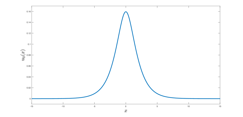
Figure 1: Numerical approximation $u_{0,1}$ for the Whitham equation.

Theorem 4.7.

(Proof of a soliton in the Whitham equation)
Let $r_{0,1}\stackrel{{\scriptstyle\mbox{\tiny{\raisebox{0.0pt}[0.0pt][0.0pt]{def}}}}}{{=}}5.72\times 10^{-9}$, then there exists a unique even solution $\tilde{u}_{1}$ to (3) in $\overline{B_{r_{0,1}}(u_{0,1})}\subset H^{l}_{e}$ for $T=0$ and $c=1.1$. Moreover, $\tilde{u}_{1}\in H^{\infty}({\mathbb{R}})\subset C^{\infty}({\mathbb{R}}).$

Proof.

The proof is a direct application of Theorem 3.1. In particular, we obtain that $\mathcal{Y}_{0}\stackrel{{\scriptstyle\mbox{\tiny{\raisebox{0.0pt}[0.0pt][0.0pt]{def}}}}}{{=}}5.24\times 10^{-9}$, $\mathcal{Z}_{1}\stackrel{{\scriptstyle\mbox{\tiny{\raisebox{0.0pt}[0.0pt][0.0pt]{def}}}}}{{=}}0.078$ and $\mathcal{Z}_{2}\stackrel{{\scriptstyle\mbox{\tiny{\raisebox{0.0pt}[0.0pt][0.0pt]{def}}}}}{{=}}1990$ satisfy (3.1). Then, one can prove that $r_{0,1}$ satisfies (33), leading to the proof of existence of $\tilde{u}_{1}$. Moreover, using that $\epsilon=0.39$ and that $\min_{\xi\in{\mathbb{R}}}|m_{0}(\xi)-c|=c-1=0.1$, we prove that $\epsilon$ and $r_{0,1}$ satisfy (47). This provides the regularity of $\tilde{u}_{1}$ (cf. Section 3.2.3). ∎

4.5.2 Case $T>0$

Similarly as the previous section, we fix $c=c_{2}\stackrel{{\scriptstyle\mbox{\tiny{\raisebox{0.0pt}[0.0pt][0.0pt]{def}}}}}{{=}}0.8$ and $T=T_{2}\stackrel{{\scriptstyle\mbox{\tiny{\raisebox{0.0pt}[0.0pt][0.0pt]{def}}}}}{{=}}0.5$, and we construct an approximate solution $u_{0,2}$ using Section 3.1. In this case, we choose ${\Omega_{0}}=(-40,40)$ and $N=800$, so that $U_{0,2}=\pi_{e}^{N}U_{0,2}$ is the Fourier series representation of $u_{0,2}$ on ${\Omega_{0}}$. The approximate solution is represented in Figure 2 below.

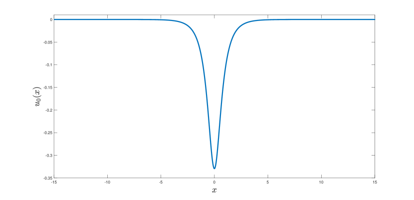
Figure 2: Numerical approximation $u_{0,2}$ for the capillary-gravity Whitham equation.

Theorem 4.8.

(Proof of a soliton in the capillary-gravity Whitham equation)
Let $r_{0,2}\stackrel{{\scriptstyle\mbox{\tiny{\raisebox{0.0pt}[0.0pt][0.0pt]{def}}}}}{{=}}8.63\times 10^{-9}$, then there exists a unique even solution $\tilde{u}_{2}$ to (3) in $\overline{B_{r_{0,2}}(u_{0,2})}\subset H^{l}_{e}$ for $T=0.5$ and $c=0.8$. Moreover, $\tilde{u}_{2}\in H^{\infty}({\mathbb{R}})\subset C^{\infty}({\mathbb{R}}).$

Proof.

We were able to prove that $\mathcal{Y}_{0}\stackrel{{\scriptstyle\mbox{\tiny{\raisebox{0.0pt}[0.0pt][0.0pt]{def}}}}}{{=}}7.13\times 10^{-9}$, $\mathcal{Z}_{1}\stackrel{{\scriptstyle\mbox{\tiny{\raisebox{0.0pt}[0.0pt][0.0pt]{def}}}}}{{=}}0.162$ and $\mathcal{Z}_{2}\stackrel{{\scriptstyle\mbox{\tiny{\raisebox{0.0pt}[0.0pt][0.0pt]{def}}}}}{{=}}1508$ satisfy (3.1). Moreover, $r_{0,2}$ satisfies (33), leading to the proof of existence of $\tilde{u}_{2}$. The regularity is obtained thanks to Proposition 2.1. ∎

5 Spectral stability

In this section, using the analysis derived in Section 5 in [8], we establish a method to prove the spectral stability of solitary wave solutions to (1). The approach is again computer-assisted and relies on the analysis of Sections 3 and 4.

We first derive sufficient conditions under which the spectral stability of solitary wave solutions is achieved. In particular, these conditions involve requirements on the spectrum of the linearization around the solitary wave. Having such conditions in mind, we derive a general computer-assisted approach to control the spetrum of the linearization. Combining these results, we are able to conclude about the stability of the solutions obtained in Theorems 4.7 and 4.8.

In this section, we do not restrict the operators to even functions anymore but instead use a subscript “e”, if necessary, to establish a restriction to the even symmetry.

5.1 Conditions for stability

Let us fix $c$ and $T$ satisfying Assumption 1 and let $\tilde{u}\in H^{\infty}({\mathbb{R}})$ be a solution to (3) obtained thanks to Theorem 3.1. In particular, assume that

$$\tilde{u}\in\overline{B_{r_{0}}(u_{0})}\subset H^{l}_{e}$$ (93)

for some $u_{0}\in H^{4}_{e}$ constructed as in Section 3.1 and $r_{0}>0.$ Moreover, $u_{0}$ satisfies Assumption 2 and it has a representation as a sequence of Fourier coefficients given by $U_{0}\in X^{4}_{e}$ and $U_{0}=\pi_{e}^{N}U_{0}$. If $T=0$, assume that

$$\|U_{0}\|_{1}+\frac{r_{0}}{4\sqrt{\nu}\sigma_{0}}<\frac{c}{2}.$$ (94)

Using the reasoning of Section 3.2.3, this implies that

$$\tilde{u}\leq\|U_{0}\|_{1}+\frac{r_{0}}{4\sqrt{\nu}\sigma_{0}}<\frac{c}{2}$$ (95)

which justifies the fact that $\tilde{u}\in H^{\infty}({\mathbb{R}})$ (cf. Proposition 2.1). The inequalities in (95) were actually proven in Theorem 4.7 for the solution $\tilde{u}_{1}$. Given this construction of $\tilde{u}$, we derive conditions under which $\tilde{u}$ is spectrally stable.

We start by re-defining our operators of interest from Section 2. Indeed, we define the following

$$\widetilde{\mathbb{L}}\stackrel{{\scriptstyle\mbox{\tiny{\raisebox{0.0pt}[0.0pt][0.0pt]{def}}}}}{{=}}\begin{cases}cI_{d}-\mathbb{M}_{T}&\text{ if }T=0\\ \mathbb{M}_{T}-cI_{d}&\text{ if }T>0\end{cases},\leavevmode\nobreak\ \leavevmode\nobreak\ \widetilde{\mathbb{G}}(u)\stackrel{{\scriptstyle\mbox{\tiny{\raisebox{0.0pt}[0.0pt][0.0pt]{def}}}}}{{=}}\begin{cases}-u^{2}&\text{ if }T=0\\ u^{2}&\text{ if }T>0\end{cases}\leavevmode\nobreak\ \text{ and }\leavevmode\nobreak\ \widetilde{\mathbb{F}}(u)\stackrel{{\scriptstyle\mbox{\tiny{\raisebox{0.0pt}[0.0pt][0.0pt]{def}}}}}{{=}}\widetilde{\mathbb{L}}u+\widetilde{\mathbb{G}}(u)$$ (96)

for all $u\in H^{l}$. These operators have a Fourier series equivalent and we define

$$\widetilde{L}\stackrel{{\scriptstyle\mbox{\tiny{\raisebox{0.0pt}[0.0pt][0.0pt]{def}}}}}{{=}}\begin{cases}cI_{d}-{M}_{T}&\text{ if }T=0\\ {M}_{T}-cI_{d}&\text{ if }T>0\end{cases},\leavevmode\nobreak\ \leavevmode\nobreak\ \widetilde{G}(U)\stackrel{{\scriptstyle\mbox{\tiny{\raisebox{0.0pt}[0.0pt][0.0pt]{def}}}}}{{=}}\begin{cases}-U*U&\text{ if }T=0\\ U*U&\text{ if }T>0\end{cases}\leavevmode\nobreak\ \text{ and }\leavevmode\nobreak\ \widetilde{F}(U)\stackrel{{\scriptstyle\mbox{\tiny{\raisebox{0.0pt}[0.0pt][0.0pt]{def}}}}}{{=}}\widetilde{L}U+\widetilde{G}(U)$$ (97)

for all $U\in X^{l}$. In particular, we abuse notation in the above and consider $M_{T}$ as a linear operator from $X^{l}$ to $\ell^{2}$ (and not from $X^{l}_{e}$ to $\ell^{2}_{e}$), represented by an infinite diagonal matrix with entries $(m_{T}(2\pi\tilde{n}))_{n\in\mathbb{Z}}$ on the diagonal. Similarly, we define $L_{\nu}$ as the diagonal matrix with entries $(l_{\nu}(2\pi\tilde{n}))_{n\in\mathbb{Z}}$ on the diagonal when applied to a sequence in $X^{l}.$

This redefinition of the zero-finding problem allows to obtain a positive definite linear part $\widetilde{\mathbb{L}}$. This set-up is useful in order to use the analysis derived in [29]. Now, let

$$D\widetilde{\mathbb{F}}_{e}(\tilde{u}):H^{l}_{e}\to L^{2}_{e}$$ (98)

be the restriction of $D\widetilde{\mathbb{F}}(\tilde{u})$ to even functions. Similarly, denote $H^{\frac{1}{2}}_{e}({\mathbb{R}})$ the restriction of $H^{\frac{1}{2}}({\mathbb{R}})$ to even function. Then, if $T>0$, recall that $D\widetilde{\mathbb{F}}_{e}(\tilde{u}):H^{\frac{1}{2}}_{e}({\mathbb{R}})\to L^{2}_{e}$ has a bounded inverse (cf. Lemma 4.4), as we assumed that $\tilde{u}$ has been obtained thanks to Theorem 3.1. Similarly, if $T=0$, then $D\widetilde{\mathbb{F}}_{e}(\tilde{u}):L^{2}_{e}\to L^{2}_{e}$ has a bounded inverse. Moreover, the analysis derived in Section 3 of [29] is applicable and we can use it to study the spectral stability of $\tilde{u}$. In particular, the reasoning of Sections 3.2 and 3.3 of [29] is readily applicable to $\partial_{x}{D}\widetilde{\mathbb{F}}(\tilde{u})$ and we resume the obtained results in the following lemma. Note that a more general approach is available at [22].

Lemma 5.1.

Assume that

(P1) $D\widetilde{\mathbb{F}}(\tilde{u})$ has a simple negative eigenvalue $\lambda^{-}$
(P2) $D\widetilde{\mathbb{F}}(\tilde{u})$ has no negative eigenvalue other than $\lambda^{-}$
(P3) 0 is a simple eigenvalue of $D\widetilde{\mathbb{F}}(\tilde{u})$.

If

$$\left(\tilde{u},D\widetilde{\mathbb{F}}_{e}(\tilde{u})^{-1}\tilde{u}\right)_{2}<0,$$ (99)

then $\tilde{u}$ is (spectrally) stable.

In the rest of this section, we prove that the condition $(\tilde{u},D\widetilde{\mathbb{F}}_{e}(\tilde{u})^{-1}\tilde{u})_{2}<0$ is always satisfied if $\tilde{u}$ is the solution described in (93). Consequently, if we can control the spectrum of $D\widetilde{\mathbb{F}}(\tilde{u})$ and verify (P1), (P2) and (P3), then we would obtain the spectral stability of $\tilde{u}$. This part is achieved in Section 5.2 below.

We first derive a preliminary lemma which will be useful in the study of the quantity $(\tilde{u},D\widetilde{\mathbb{F}}_{e}(\tilde{u})^{-1}\tilde{u})_{2}.$

Lemma 5.2.

Let $\mathcal{L}_{T}:L^{2}\to H^{\frac{1}{2}}({\mathbb{R}})$ be defined as

$$\mathcal{L}_{T} \stackrel{{\scriptstyle\mbox{\tiny{\raisebox{0.0pt}[0.0pt][0.0pt]{def}}}}}{{=}}\begin{cases}\widetilde{\mathbb{L}}^{-1}-\frac{1}{c}I_{d}&\text{ if }T=0\\ \widetilde{\mathbb{L}}^{-1}&\text{ if }T>0.\end{cases}$$

Then $\mathcal{L}_{T}\tilde{\mathbb{u}}:L^{2}\to L^{2}$ is compact.

Proof.

First, notice that $\mathcal{L}_{0}$ has a symbol given by

$$l_{0}(\xi)\stackrel{{\scriptstyle\mbox{\tiny{\raisebox{0.0pt}[0.0pt][0.0pt]{def}}}}}{{=}}\frac{1}{c-m_{0}(\xi)}-\frac{1}{c}$$

for all $\xi\in{\mathbb{R}}.$ In particular, since $c>1$ when $T=0$ (cf. Assumption 1), $l_{0}(\xi)>0$ for all $\xi\in{\mathbb{R}}$ and $l_{0}(\xi)=O(\frac{1}{\sqrt{|\xi|}})$ as $\xi\to\infty$. This implies that $\mathcal{L}_{T}:L^{2}\to H^{\frac{1}{2}}({\mathbb{R}})$ is a bounded, linear and invertible operator for all $T\geq 0$. Then, using the reasoning of Lemma 3.1 in [8] and the fact that $H^{\frac{1}{2}}_{0}(\Omega)$ is compactly embedded in $L^{2}(\Omega)$ for a Lipschitz bounded domain $\Omega$ (see [24] for instance), we obtain that $\mathcal{L}_{T}\tilde{\mathbb{u}}:L^{2}\to L^{2}$ is compact. ∎

Using the previous lemma, we prove that $(\tilde{u},D\widetilde{\mathbb{F}}_{e}(\tilde{u})^{-1}\tilde{u})_{2}<0$.

Theorem 5.3.

Let $\tilde{u}$ be the solution to (3) described in (93). In particular, $\tilde{u}<\frac{c}{2}$ if $T=0$. Then,

$$(\tilde{u},D\widetilde{\mathbb{F}}_{e}(\tilde{u})^{-1}\tilde{u})_{2}<0.$$ (100)

Proof.

By assumption, recall that $\tilde{u}\in H^{\infty}({\mathbb{R}})$ satisfies $\widetilde{\mathbb{L}}\tilde{u}+\widetilde{\mathbb{G}}(\tilde{u})=0$. Therefore,

$$\widetilde{\mathbb{L}}\tilde{u}+2\widetilde{\mathbb{G}}(\tilde{u})=D\widetilde{\mathbb{F}}_{e}(\tilde{u})\tilde{u}=\widetilde{\mathbb{G}}(\tilde{u})=-\widetilde{\mathbb{L}}\tilde{u},$$

where $D\widetilde{\mathbb{F}}_{e}(\tilde{u})$ is introduced in (98). In particular, we have

$$\tilde{u}=-\widetilde{\mathbb{L}}^{-1}D\widetilde{\mathbb{F}}_{e}(\tilde{u})\tilde{u}.$$

Now, notice that

$$(\tilde{u},D\widetilde{\mathbb{F}}_{e}(\tilde{u})^{-1}\tilde{u})_{2}=-(\widetilde{\mathbb{L}}^{-1}D\widetilde{\mathbb{F}}_{e}(\tilde{u})\tilde{u},D\widetilde{\mathbb{F}}_{e}(\tilde{u})^{-1}\tilde{u})_{2}=-(\tilde{u},D\widetilde{\mathbb{F}}_{e}(\tilde{u})\widetilde{\mathbb{L}}^{-1}D\widetilde{\mathbb{F}}_{e}(\tilde{u})^{-1}\tilde{u})_{2}$$

as $\widetilde{\mathbb{L}}^{-1}$ and $D\widetilde{\mathbb{F}}_{e}(\tilde{u})$ are self-adjoint on $L^{2}.$ Let $w\stackrel{{\scriptstyle\mbox{\tiny{\raisebox{0.0pt}[0.0pt][0.0pt]{def}}}}}{{=}}D\widetilde{\mathbb{F}}_{e}(\tilde{u})^{-1}\tilde{u}$, then we have

$$(\tilde{u},D\widetilde{\mathbb{F}}_{e}(\tilde{u})^{-1}\tilde{u})_{2}=-(w,D\widetilde{\mathbb{F}}_{e}(\tilde{u})^{2}\widetilde{\mathbb{L}}^{-1}w)_{2}.$$ (101)

Suppose first that $T>0$, then

$$D\widetilde{\mathbb{F}}_{e}(\tilde{u})^{2}=(\widetilde{\mathbb{L}}+2\tilde{\mathbb{u}})(\widetilde{\mathbb{L}}+2\tilde{\mathbb{u}})=\widetilde{\mathbb{L}}(I_{d}+2\widetilde{\mathbb{L}}^{-1}\tilde{\mathbb{u}})(I_{d}+2\tilde{\mathbb{u}}\widetilde{\mathbb{L}}^{-1})\widetilde{\mathbb{L}}=\widetilde{\mathbb{L}}\mathbb{P}\mathbb{P}^{*}\widetilde{\mathbb{L}}$$

where $\mathbb{P}\stackrel{{\scriptstyle\mbox{\tiny{\raisebox{0.0pt}[0.0pt][0.0pt]{def}}}}}{{=}}I_{d}+2\widetilde{\mathbb{L}}^{-1}\tilde{\mathbb{u}}$. Notice that $\mathbb{P}$ is invertible by construction as $D\widetilde{\mathbb{F}}_{e}(\tilde{u})$ is invertible by Lemma 4.4. Then, using (101), we obtain

$$(\tilde{u},D\widetilde{\mathbb{F}}_{e}(\tilde{u})^{-1}\tilde{u})_{2}=(w,\widetilde{\mathbb{L}}\mathbb{P}\mathbb{P}^{*}w)_{2}.$$

In particular, since $T>0$, we have that $\widetilde{\mathbb{L}}=\mathbb{M}_{T}-cI_{d}$ and, using Lemma 5.2, $\widetilde{\mathbb{L}}^{-1}\tilde{\mathbb{u}}:L^{2}\to L^{2}$ is compact. Therefore,

$$\mathbb{P}\mathbb{P}^{*}=I_{d}+2\widetilde{\mathbb{L}}^{-1}\tilde{\mathbb{u}}+\tilde{\mathbb{u}}\widetilde{\mathbb{L}}^{-1}+4\widetilde{\mathbb{L}}^{-1}\tilde{\mathbb{u}}^{2}\widetilde{\mathbb{L}}^{-1}=I_{d}+\mathbb{K}$$

where $\mathbb{K}\stackrel{{\scriptstyle\mbox{\tiny{\raisebox{0.0pt}[0.0pt][0.0pt]{def}}}}}{{=}}2\widetilde{\mathbb{L}}^{-1}\tilde{\mathbb{u}}+2\tilde{\mathbb{u}}\widetilde{\mathbb{L}}^{-1}+4\widetilde{\mathbb{L}}^{-1}\tilde{\mathbb{u}}^{2}\widetilde{\mathbb{L}}^{-1}:L^{2}\to L^{2}$ is a self-adjoint compact operator. Consequently, there exists an orthonormal basis of eigenfunctions of $\mathbb{K}$ that we denote $(v_{i})_{i\in\mathbb{N}}$. But as $\mathbb{P}\mathbb{P}^{*}=I_{d}+\mathbb{K}$, then $(v_{i})_{i\in\mathbb{N}}$ are also eigenfunctions of $\mathbb{P}\mathbb{P}^{*}$ associated to eigenvalues $(\mu_{i})_{i\in\mathbb{N}}$, where $\mu_{i}>0$ for all $i\in\mathbb{N}$ as $\mathbb{P}\mathbb{P}^{*}$ is symmetric positive definite (as $\mathbb{P}$ is invertible).

Now, let $v=\widetilde{\mathbb{L}}^{\frac{1}{2}}w$ (which is well-defined as $\widetilde{\mathbb{L}}$ is a positive operator). Then clearly $v\in L^{2}$ as $\tilde{u}\in H^{\infty}({\mathbb{R}})$ and $v=\sum_{i\in\mathbb{N}}\alpha_{i}v_{i}$ for some real coefficients $(\alpha_{i})_{i\in\mathbb{N}}$. Moreover, we have

$$(\tilde{u},D\widetilde{\mathbb{F}}_{e}(\tilde{u})^{-1}\tilde{u})_{2} =-(v,\widetilde{\mathbb{L}}^{\frac{1}{2}}\mathbb{P}\mathbb{P}^{*}\widetilde{\mathbb{L}}^{-\frac{1}{2}}v)$$

$$=-\sum_{i,j\in\mathbb{N}}\alpha_{i}\alpha_{j}(v_{i},\widetilde{\mathbb{L}}^{\frac{1}{2}}\mathbb{P}\mathbb{P}^{*}\widetilde{\mathbb{L}}^{-\frac{1}{2}}v_{j})$$

$$=-\sum_{i,j\in\mathbb{N}}\alpha_{i}\alpha_{j}(v_{i},\mu_{j}v_{j})$$

$$=-\sum_{i\in\mathbb{N}}\alpha_{i}^{2}\mu_{i}<0$$

as $(v_{i})_{i\in\mathbb{N}}$ clearly are eigenfunctions of $\widetilde{\mathbb{L}}^{\frac{1}{2}}\mathbb{P}\mathbb{P}^{*}\widetilde{\mathbb{L}}^{-\frac{1}{2}}$ by definition. This proves the result if $T>0$.

Now, let us assume that $T=0$. First, recall that $\tilde{u}<\frac{c}{2}$ by assumption. In particular, this implies that $(I_{d}-\frac{2}{c}\tilde{\mathbb{u}})^{-1}:L^{2}\to L^{2}$ is a positive bounded linear operator. Then, notice that

$$D\widetilde{\mathbb{F}}_{e}(\tilde{u})^{2} =\widetilde{\mathbb{L}}(I_{d}-2\widetilde{\mathbb{L}}^{-1}\tilde{\mathbb{u}})(I_{d}-2\tilde{\mathbb{u}}\widetilde{\mathbb{L}}^{-1})\widetilde{\mathbb{L}}$$

$$=\widetilde{\mathbb{L}}(I_{d}-\frac{2}{c}\tilde{\mathbb{u}})(I_{d}-2(I_{d}-\frac{2}{c}\tilde{\mathbb{u}})^{-1}\mathcal{L}_{0}\tilde{\mathbb{u}})(I_{d}-2\tilde{\mathbb{u}}\mathcal{L}_{0}(I_{d}-\frac{2}{c}\tilde{\mathbb{u}})^{-1})(I_{d}-\frac{2}{c}\tilde{\mathbb{u}})\widetilde{\mathbb{L}}$$

$$=\widehat{\mathbb{L}}\mathbb{P}\mathbb{P}^{*}\widehat{\mathbb{L}}^{*}$$

where

$$\mathbb{P} \stackrel{{\scriptstyle\mbox{\tiny{\raisebox{0.0pt}[0.0pt][0.0pt]{def}}}}}{{=}}I_{d}-2(I_{d}-\frac{2}{c}\tilde{\mathbb{u}})^{-1}\mathcal{L}_{0}\tilde{\mathbb{u}}$$

$$\widehat{\mathbb{L}} \stackrel{{\scriptstyle\mbox{\tiny{\raisebox{0.0pt}[0.0pt][0.0pt]{def}}}}}{{=}}\widetilde{\mathbb{L}}(I_{d}-\frac{2}{c}\tilde{\mathbb{u}})$$

and $\mathcal{L}_{0}$ is defined in Lemma 5.2. In particular, the aforementioned lemma provides that $\mathcal{L}_{0}\tilde{\mathbb{u}}:L^{2}\to L^{2}$ is compact. Therefore, $2(I_{d}-\frac{2}{c}\tilde{\mathbb{u}})^{-1}\mathcal{L}_{0}\tilde{\mathbb{u}}:L^{2}\to L^{2}$ is compact as $(I_{d}-\frac{2}{c}\tilde{\mathbb{u}})^{-1}:L^{2}\to L^{2}$ is bounded. Therefore, similarly as above, we can prove that there exists an orthonormal basis of eigenfunctions $(v_{i})_{i\in\mathbb{N}}$ of $\mathbb{P}\mathbb{P}^{*}$ in $L^{2}$ associated to stricly positive eigenvalues $(\mu_{i})_{i\in\mathbb{N}}$ (using that $\mathbb{P}$ is invertible). Therefore, using (101), we have

$$(\tilde{u},D\widetilde{\mathbb{F}}_{e}(\tilde{u})^{-1}\tilde{u})_{2} =-(w,\widehat{\mathbb{L}}\mathbb{P}\mathbb{P}^{*}\widehat{\mathbb{L}}^{*}\widetilde{\mathbb{L}}^{-1}w)_{2}$$

$$=-(\widetilde{\mathbb{L}}w,(I_{d}-\frac{2}{c}\tilde{\mathbb{u}})\mathbb{P}\mathbb{P}^{*}(I_{d}-\frac{2}{c}\tilde{\mathbb{u}})w)_{2}$$

$$=-(v,\widetilde{\mathbb{L}}^{\frac{1}{2}}(I_{d}-\frac{2}{c}\tilde{\mathbb{u}})\mathbb{P}\mathbb{P}^{*}(I_{d}-\frac{2}{c}\tilde{\mathbb{u}})\widetilde{\mathbb{L}}^{-\frac{1}{2}}v)_{2}$$

where $v=\widetilde{\mathbb{L}}^{\frac{1}{2}}w$. Now, let $i\in\mathbb{N}$ and denote $\mathbb{T}\stackrel{{\scriptstyle\mbox{\tiny{\raisebox{0.0pt}[0.0pt][0.0pt]{def}}}}}{{=}}I_{d}-\frac{2}{c}\tilde{\mathbb{u}}$. Then

$$\widetilde{\mathbb{L}}^{\frac{1}{2}}\mathbb{T}\mathbb{P}\mathbb{P}^{*}\mathbb{T}\widetilde{\mathbb{L}}^{-\frac{1}{2}}w_{i}=\mu_{i}\mathbb{T}^{2}w_{i}$$ (102)

where $w_{i}\stackrel{{\scriptstyle\mbox{\tiny{\raisebox{0.0pt}[0.0pt][0.0pt]{def}}}}}{{=}}\mathbb{T}^{-1}v_{i}$. Now, since $\mathbb{T}:L^{2}\to L^{2}$ is a bounded linear operator with a bounded inverse, then $(w_{i})_{i\in\mathbb{N}}$ also forms a basis for $L^{2}.$ In particular, assume that $v=\sum_{i\in\mathbb{N}}\alpha_{i}w_{i}$ for some real constants $(\alpha_{i})_{i\in\mathbb{N}}$. Then, using (102), we get

$$-(v,\widetilde{\mathbb{L}}^{\frac{1}{2}}(I_{d}-\frac{2}{c}\tilde{\mathbb{u}})\mathbb{P}\mathbb{P}^{*}(I_{d}-\frac{2}{c}\tilde{\mathbb{u}})\widetilde{\mathbb{L}}^{-\frac{1}{2}}v)_{2} =-\sum_{i,j\in\mathbb{N}}\alpha_{i}\alpha_{j}\mu_{i}(w_{j},\mathbb{T}^{2}w_{i})_{2}$$

$$=-\sum_{i,j\in\mathbb{N}}\alpha_{i}\alpha_{j}\mu_{i}(v_{j},v_{i})_{2}$$

$$=-\sum_{i\in\mathbb{N}}\alpha_{i}^{2}\mu_{i}<0$$

where we used that $\mathbb{T}w_{i}=v_{i}$ and that $\mathbb{T}$ is self-adjoint by construction. This proves the theorem. ∎

Using the previous theorem, the spectral stability of $\tilde{u}$ depends only on the negative spectrum of $D\widetilde{\mathbb{F}}(\tilde{u})$. Consequently, we recall some tools from [8] in order to study eigenvalue problems and we prove the spectral stability of the solutions $\tilde{u}_{1}$ and $\tilde{u}_{2}$ given in Theorems 4.7 and 4.8 respectively.

5.2 Proof of eigencouples of $D\widetilde{\mathbb{F}}(\tilde{u})$

First, notice that $D\widetilde{\mathbb{F}}(\tilde{u})$ only possesses real eigenvalues as it is self-adjoint on $L^{2}$. Then, similarly as what was achieved in Section 5 in [8], the goal is to set-up a zero finding problem to prove eigencouples of $D\widetilde{\mathbb{F}}(\tilde{u}).$ Following Lemma 5.1, it is enough to study the non-positive part of the spectrum of $D\widetilde{\mathbb{F}}(\tilde{u})$ in order to conclude about stability. In particular, we prove that the non-positive part of the spectrum of $D\widetilde{\mathbb{F}}(\tilde{u})$ only contains eigenvalues with finite multiplicity.

Lemma 5.4.

Let $\sigma_{0}$ be defined in Lemma 4.1 and let $\lambda_{\max}>0$ be defined as

$$\lambda_{\max}\stackrel{{\scriptstyle\mbox{\tiny{\raisebox{0.0pt}[0.0pt][0.0pt]{def}}}}}{{=}}\begin{cases}\min\left\{\sigma_{0},\leavevmode\nobreak\ c-2\left(\|U_{0}\|_{1}+\frac{r_{0}}{4\sqrt{\nu}\sigma_{0}}\right)\right\}&\text{ if }T=0\\ \sigma_{0}&\text{ if }T>0.\end{cases}$$ (103)

Let $\lambda<\lambda_{\max}$ be such that $D\widetilde{\mathbb{F}}(\tilde{u})-\lambda I_{d}$ is non-invertible. Then $\lambda$ is an eigenvalue of $D\widetilde{\mathbb{F}}(\tilde{u})$ with finite multiplicity.

Proof.

First, since $\lambda<\lambda_{\max}\leq\sigma_{0}$, we obtain that $\mathbb{L}_{\lambda}\stackrel{{\scriptstyle\mbox{\tiny{\raisebox{0.0pt}[0.0pt][0.0pt]{def}}}}}{{=}}\widetilde{\mathbb{L}}-\lambda I_{d}$ is a positive definite linear operator and is invertible. Suppose that $T>0$. Then

$$D\widetilde{\mathbb{F}}(\tilde{u})-\lambda I_{d}=\mathbb{L}_{\lambda}+2\tilde{\mathbb{u}}=\mathbb{L}_{\lambda}\left(I_{d}+2\mathbb{L}_{\lambda}^{-1}\tilde{\mathbb{u}}\right).$$

Moreover, using the proof of Lemma 5.2, we obtain that $2\mathbb{L}_{\lambda}^{-1}\tilde{\mathbb{u}}:L^{2}\to L^{2}$ is compact and therefore $D\widetilde{\mathbb{F}}(\tilde{u})-\lambda I_{d}$ is a Fredholm operator. We conclude the proof for the case $T>0$ using the Fredholm alternative. Now, if $T=0$, then

$$D\widetilde{\mathbb{F}}(\tilde{u})-\lambda I_{d}=\mathbb{L}_{\lambda}\left(I_{d}-2\mathbb{L}_{\lambda}^{-1}\tilde{\mathbb{u}}\right)=\mathbb{L}_{\lambda}(I_{d}-\frac{2}{c-\lambda}\tilde{\mathbb{u}})\left(I_{d}-2(I_{d}-\frac{2}{c-\lambda}\tilde{\mathbb{u}})^{-1}\left(\mathbb{L}_{\lambda}^{-1}-\frac{1}{c-\lambda}I_{d}\right)\tilde{\mathbb{u}}\right).$$

Now, using (95), we have that

$$\tilde{u}\leq\|U_{0}\|_{1}+\frac{r_{0}}{4\sqrt{\nu}\sigma_{0}}\leq\frac{c-\lambda_{\max}}{2}<\frac{c-\lambda}{2}.$$

as $\lambda<\lambda_{\max}$. Therefore, since $\tilde{u}$ is smooth, we have that $(I_{d}-\frac{2}{c-\lambda}\tilde{\mathbb{u}})^{-1}:L^{2}\to L^{2}$ is bounded. Moreover, using the proof of Lemma 5.2, we obtain that $\left(\mathbb{L}_{\lambda}^{-1}-\frac{1}{c-\lambda}I_{d}\right)\tilde{\mathbb{u}}:L^{2}\to L^{2}$ is compact, which implies that $2(I_{d}-\frac{2}{c-\lambda}\tilde{\mathbb{u}})^{-1}\left(\mathbb{L}_{\lambda}^{-1}-\frac{1}{c-\lambda}I_{d}\right)\tilde{\mathbb{u}}:L^{2}\to L^{2}$ is compact as well. Again, it implies that $D\widetilde{\mathbb{F}}(\tilde{u})-\lambda I_{d}$ is a Fredholm operator, which concludes the proof. ∎

Using the above lemma combined with Lemma 5.1, we obtain that we can study the stability of $\tilde{u}$ by controlling the non-positive eigenvalues of $D\widetilde{\mathbb{F}}(\tilde{u})$. Consequently, we expose a computer-assisted strategy to prove the existence of an eigencouple $(\tilde{\lambda},\tilde{\psi})$, given an approximation $(\lambda_{0},\psi_{0})$.

Let $\psi_{0}\in H^{l}_{\Omega_{0}}$ be an approximate eigenvector of $D\widetilde{\mathbb{F}}(\tilde{u})$ associated to an approximate eigenvalue $\lambda_{0}\leq 0$. Moreover, using the construction presented in Section 3.1, we assume that $\psi_{0}$ is determined numerically and that there exists $\Psi_{0}\in X^{4}$ such that

$$\psi_{0}=\gamma^{\dagger}(\Psi_{0})\in H^{4}_{{\Omega_{0}}}\text{ with }\leavevmode\nobreak\ \leavevmode\nobreak\ \Psi_{0}=\pi^{N}\Psi_{0},$$

where $\pi^{N}$ is defined in (34). Given $\lambda\leq 0$, we have

$$|m_{T}(\xi)-c|-\lambda \geq\sigma_{0}-\lambda>0$$ (104)

for all $\xi\in{\mathbb{R}}$. Therefore, for all $\lambda\leq 0$, we define the linear operator $\mathbb{L}_{\lambda}$ as follows

$$\mathbb{L}_{\lambda}\stackrel{{\scriptstyle\mbox{\tiny{\raisebox{0.0pt}[0.0pt][0.0pt]{def}}}}}{{=}}\widetilde{\mathbb{L}}-\lambda I_{d}$$ (105)

and define the associated Hilbert space $H^{l}_{\lambda}$ as in (11) with norm $\|u\|_{H^{l}_{\lambda}}\stackrel{{\scriptstyle\mbox{\tiny{\raisebox{0.0pt}[0.0pt][0.0pt]{def}}}}}{{=}}\|\mathbb{L}_{\lambda}u\|_{2}$ for all $u\in H^{l}_{\lambda}$. $H^{l}_{\lambda}$ is well-defined as ${\mathbb{L}}_{\lambda}$ is a definite positive operator (using (104)) so $\mathbb{L}_{\lambda}:H^{l}_{\lambda}\to L^{2}$ is an isometric isomorphism. Moreover, denote by $H_{1}\stackrel{{\scriptstyle\mbox{\tiny{\raisebox{0.0pt}[0.0pt][0.0pt]{def}}}}}{{=}}\mathbb{R}\times H^{l}_{\lambda_{0}}$ and $H_{2}\stackrel{{\scriptstyle\mbox{\tiny{\raisebox{0.0pt}[0.0pt][0.0pt]{def}}}}}{{=}}\mathbb{R}\times L^{2}$ the Hilbert spaces endowed respectively with the norms

$$\|(\nu,u)\|_{H_{1}}\stackrel{{\scriptstyle\mbox{\tiny{\raisebox{0.0pt}[0.0pt][0.0pt]{def}}}}}{{=}}\left(|\nu|^{2}+\|u\|_{H^{l}_{\lambda_{0}}}^{2}\right)^{\frac{1}{2}}\leavevmode\nobreak\ \leavevmode\nobreak\ \text{ and }\leavevmode\nobreak\ \leavevmode\nobreak\ \|(\nu,u)\|_{H_{2}}\stackrel{{\scriptstyle\mbox{\tiny{\raisebox{0.0pt}[0.0pt][0.0pt]{def}}}}}{{=}}\left(|\nu|^{2}+\|u\|_{2}^{2}\right)^{\frac{1}{2}}.$$

In particular, we have

$$x_{0}\stackrel{{\scriptstyle\mbox{\tiny{\raisebox{0.0pt}[0.0pt][0.0pt]{def}}}}}{{=}}(\lambda_{0},\psi_{0})\in H_{1}$$ (106)

by construction. Denote $x=(\nu,u)\in H_{1}$ and define the augmented zero finding problem $\overline{\mathbb{F}}:H_{1}\to H_{2}$ as

$$\overline{\mathbb{F}}(x)\stackrel{{\scriptstyle\mbox{\tiny{\raisebox{0.0pt}[0.0pt][0.0pt]{def}}}}}{{=}}\begin{pmatrix}(\psi_{0}-u,\psi_{0})_{2}\\ D\widetilde{\mathbb{F}}(\tilde{u})u-\nu u\end{pmatrix}=0$$ (107)

for all $x=(\nu,u)\in H_{1}$. Zeros of $\overline{\mathbb{F}}$ are equivalently eigencouples of $D\widetilde{\mathbb{F}}(\tilde{u}).$ Moreover, similarly as in [8], we define $\overline{\mathbb{F}}_{0}:H_{1}\to H_{2}$ as

$$\overline{\mathbb{F}}_{0}(x)\stackrel{{\scriptstyle\mbox{\tiny{\raisebox{0.0pt}[0.0pt][0.0pt]{def}}}}}{{=}}\begin{pmatrix}(\psi_{0}-u,\psi_{0})_{2}\\ D\widetilde{\mathbb{F}}({u}_{0})u-\nu u\end{pmatrix}.$$

Note that the analysis derived in [8] does not readily allow to investigate $D\overline{\mathbb{F}}(x_{0})$ as $\tilde{u}$ does not necessarily have a support contained on ${\Omega_{0}}$. However, the theory applies to $D\overline{\mathbb{F}}_{0}(x_{0})$. Moreover, using that $\|\tilde{u}-u_{0}\|_{l}\leq r_{0}$ by assumption, we can build an approximate inverse for $D\overline{\mathbb{F}}_{0}(x_{0})$ and use the control on $\|\tilde{u}-u_{0}\|_{l}$ to obtain rigorous estimates for $D\overline{\mathbb{F}}(x_{0})$ (cf. Section 5 in [8]).

Now, the map $\overline{\mathbb{F}}_{0}$ has a periodic correspondence on ${\Omega_{0}}$. Indeed, given $\lambda\leq 0$, define $L_{\lambda}$ as

$$L_{\lambda}\stackrel{{\scriptstyle\mbox{\tiny{\raisebox{0.0pt}[0.0pt][0.0pt]{def}}}}}{{=}}\tilde{L}-\lambda I_{d}.$$ (108)

Then, define $X^{l}_{\lambda_{0}}$ to be the following Hilbert space defined as

$$X^{l}_{\lambda}\stackrel{{\scriptstyle\mbox{\tiny{\raisebox{0.0pt}[0.0pt][0.0pt]{def}}}}}{{=}}\left\{U\in\ell^{2}(\mathbb{Z}),\leavevmode\nobreak\ \leavevmode\nobreak\ \|U\|_{X^{l}_{\lambda}}\stackrel{{\scriptstyle\mbox{\tiny{\raisebox{0.0pt}[0.0pt][0.0pt]{def}}}}}{{=}}\|L_{\lambda}U\|_{2}<\infty\right\}.$$ (109)

Moreover, define the Hilbert spaces $X_{1}\stackrel{{\scriptstyle\mbox{\tiny{\raisebox{0.0pt}[0.0pt][0.0pt]{def}}}}}{{=}}\mathbb{R}\times X^{l}_{\lambda_{0}}$ and $X_{2}\stackrel{{\scriptstyle\mbox{\tiny{\raisebox{0.0pt}[0.0pt][0.0pt]{def}}}}}{{=}}\mathbb{R}\times\ell^{2}$ associated to their norms

$$\|(\nu,U)\|_{X_{1}}\stackrel{{\scriptstyle\mbox{\tiny{\raisebox{0.0pt}[0.0pt][0.0pt]{def}}}}}{{=}}\left(|\nu|^{2}+|{\Omega_{0}}|\|U\|_{X^{l}_{\lambda_{0}}}^{2}\right)^{\frac{1}{2}}\leavevmode\nobreak\ \leavevmode\nobreak\ \text{and}\leavevmode\nobreak\ \leavevmode\nobreak\ \|(\nu,U)\|_{X_{2}}\stackrel{{\scriptstyle\mbox{\tiny{\raisebox{0.0pt}[0.0pt][0.0pt]{def}}}}}{{=}}\left(|\nu|^{2}+|{\Omega_{0}}|\|U\|_{2}^{2}\right)^{\frac{1}{2}}.$$

Finally, we define a corresponding operator $\overline{F}:X_{1}\to X_{2}$ as

$$\overline{F}(\nu,U)\stackrel{{\scriptstyle\mbox{\tiny{\raisebox{0.0pt}[0.0pt][0.0pt]{def}}}}}{{=}}\begin{pmatrix}|{\Omega_{0}}|(\Psi_{0}-U,\Psi_{0})_{2}\\ D\widetilde{F}(u_{0})U-\nu U\end{pmatrix}.$$

At this point, we require the construction of an approximate inverse $D\overline{\mathbb{F}}_{0}(x_{0}):H_{1}\to H_{2}$. Let $\overline{\mathbb{L}}:H_{1}\to H_{2}$ be defined as follows

$$\overline{\mathbb{L}}\stackrel{{\scriptstyle\mbox{\tiny{\raisebox{0.0pt}[0.0pt][0.0pt]{def}}}}}{{=}}\begin{pmatrix}1&0\\ 0&\mathbb{L}_{\lambda_{0}}\end{pmatrix}.$$

Then, by construction $\overline{\mathbb{L}}$ is an isometric isomorphism between $H_{1}$ and $H_{2}$. Moreover, denote $\overline{\mathbb{1}}_{\Omega_{0}}:H_{2}\to H_{2}$, $\overline{\pi}^{N}:X_{2}\to X_{2}$ and $\overline{\pi}_{N}:X_{2}\to X_{2}$ the projection operators defined as

$$\overline{\mathbb{1}}_{\Omega_{0}}\stackrel{{\scriptstyle\mbox{\tiny{\raisebox{0.0pt}[0.0pt][0.0pt]{def}}}}}{{=}}\begin{pmatrix}1&0\\ 0&\mathbb{1}_{\Omega_{0}}\end{pmatrix},\leavevmode\nobreak\ \leavevmode\nobreak\ \overline{\pi}^{N}\stackrel{{\scriptstyle\mbox{\tiny{\raisebox{0.0pt}[0.0pt][0.0pt]{def}}}}}{{=}}\begin{pmatrix}1&0\\ 0&\pi^{N}\end{pmatrix}\text{ and }\leavevmode\nobreak\ \overline{\pi}_{N}\stackrel{{\scriptstyle\mbox{\tiny{\raisebox{0.0pt}[0.0pt][0.0pt]{def}}}}}{{=}}\begin{pmatrix}0&0\\ 0&\pi_{N}\end{pmatrix}.$$

Now, we build an approximate inverse for $D\overline{\mathbb{F}}_{0}(x_{0}):H_{1}\to H_{2}$ following the construction of Section 3.2. Indeed, we build a linear operator $\overline{B}_{T}\stackrel{{\scriptstyle\mbox{\tiny{\raisebox{0.0pt}[0.0pt][0.0pt]{def}}}}}{{=}}\overline{B}^{N}_{T}+\overline{\pi}_{N}\begin{pmatrix}0&0\\ 0&\mathbb{W}_{T}\end{pmatrix}:X_{2}\to X_{2}$ such that $\overline{B}^{N}_{T}=\overline{\pi}^{N}\overline{B}^{N}_{T}\overline{\pi}^{N}$ and define $\overline{A}_{T}:X_{1}\to X_{2}$ as

$$\overline{A}_{T}\stackrel{{\scriptstyle\mbox{\tiny{\raisebox{0.0pt}[0.0pt][0.0pt]{def}}}}}{{=}}\begin{pmatrix}1&0\\ 0&L_{\lambda_{0}}^{-1}\end{pmatrix}\overline{B}_{T}.$$ (110)

Intuitively, $\overline{A}_{T}$ is an approximation of the inverse of $D\overline{F}(\lambda_{0},\Psi_{0})$. Moreover, define $W_{T}=e_{0}$ (where $e_{0}$ is given in (42)) for all $T>0$ and $W_{0}=\pi^{N}W_{0}\in\ell^{1}$. $W_{0}$ is a sequence chosen such that $W_{0}=\pi^{N}W_{0}$ and

$$W_{0}*(e_{0}-\frac{2}{c-\lambda_{0}}U_{0})\approx e_{0}.$$

Moreover, denote $\overline{B}_{T}^{N}\stackrel{{\scriptstyle\mbox{\tiny{\raisebox{0.0pt}[0.0pt][0.0pt]{def}}}}}{{=}}\begin{pmatrix}b_{1,1}&B_{1,2}^{*}\\ B_{2,1}&B_{2,2}\end{pmatrix}$ where $b_{1,1}\in{\mathbb{R}}$, $B_{2,2}=\pi^{N}B_{2,2}\pi^{N}$ and $B_{1,2},B_{2,1}\in\ell^{2}$ are such that $B_{1,2}=\pi^{N}B_{1,2}$ and $B_{2,1}=\pi^{N}B_{2,1}$.

Let us denote $\mathcal{B}_{{\Omega_{0}}}(H_{2})$ the following set

$$\mathcal{B}_{{\Omega_{0}}}(H_{2})\stackrel{{\scriptstyle\mbox{\tiny{\raisebox{0.0pt}[0.0pt][0.0pt]{def}}}}}{{=}}\{\overline{\mathbb{B}}\in\mathcal{B}(H_{2}),\leavevmode\nobreak\ \overline{\mathbb{B}}=\overline{\mathbb{1}}_{\Omega_{0}}\overline{\mathbb{B}}\overline{\mathbb{1}}_{\Omega_{0}}\}$$

where $\mathcal{B}(H_{2})$ is the set of linear bounded operators on $H_{2}$. Moreover, define $H_{2,{\Omega_{0}}}$ as

$$H_{2,{\Omega_{0}}}\stackrel{{\scriptstyle\mbox{\tiny{\raisebox{0.0pt}[0.0pt][0.0pt]{def}}}}}{{=}}\{x\in H_{2},\leavevmode\nobreak\ x=\overline{\mathbb{1}}_{\Omega_{0}}x\}.$$

Recall the definition of the following maps introduced in [8] $\overline{\gamma}:H_{2}\to X_{2}$, $\overline{\gamma}^{\dagger}:X_{2}\to H_{2}$, $\overline{\Gamma}:\mathcal{B}(H_{2})\to\mathcal{B}(X_{2})$ and $\overline{\Gamma}^{\dagger}:\mathcal{B}(X_{2})\to\mathcal{B}(H_{2})$

$$\overline{\gamma}\stackrel{{\scriptstyle\mbox{\tiny{\raisebox{0.0pt}[0.0pt][0.0pt]{def}}}}}{{=}}\begin{pmatrix}1&0\\ 0&\gamma\end{pmatrix}\leavevmode\nobreak\ \leavevmode\nobreak\ \text{ and }\leavevmode\nobreak\ \leavevmode\nobreak\ \overline{\gamma}^{\dagger}\stackrel{{\scriptstyle\mbox{\tiny{\raisebox{0.0pt}[0.0pt][0.0pt]{def}}}}}{{=}}\begin{pmatrix}1&0\\ 0&\gamma^{\dagger}\end{pmatrix}$$

$$\overline{\Gamma}\left(\overline{\mathbb{B}}\right)\stackrel{{\scriptstyle\mbox{\tiny{\raisebox{0.0pt}[0.0pt][0.0pt]{def}}}}}{{=}}\overline{\gamma}\overline{\mathbb{B}}\overline{\gamma}^{\dagger}\leavevmode\nobreak\ \leavevmode\nobreak\ \text{ and }\leavevmode\nobreak\ \leavevmode\nobreak\ \overline{\Gamma}^{\dagger}\left(\overline{B}\right)\stackrel{{\scriptstyle\mbox{\tiny{\raisebox{0.0pt}[0.0pt][0.0pt]{def}}}}}{{=}}\overline{\gamma}^{\dagger}\overline{B}\overline{\gamma}$$

for all $\overline{\mathbb{B}}\in\mathcal{B}(H_{2})$ and $\overline{B}\in X_{2}$. Then, we recall Lemma 5.1 in [8], which provides a one to one relationship between bounded linear operators on $X_{2}$ and the ones in $\mathcal{B}_{{\Omega_{0}}}(H_{2})$.

Lemma 5.5.

The map $\overline{\gamma}:H_{2,{\Omega_{0}}}\to X_{2}$ (respectively $\overline{\Gamma}:\mathcal{B}_{\Omega_{0}}(H_{2})\to\mathcal{B}(X_{2})$) is an isometric isomorphism whose inverse is $\overline{\gamma}^{\dagger}:X_{2}\to H_{2,{\Omega_{0}}}$ (respectively $\overline{\Gamma}^{\dagger}:\mathcal{B}(X_{2})\to\mathcal{B}_{\Omega_{0}}(H_{2})$). In particular,

$$\|(\nu,u)\|_{H_{2}}=\|(\nu,U)\|_{X_{2}}\leavevmode\nobreak\ \leavevmode\nobreak\ \text{ and }\leavevmode\nobreak\ \leavevmode\nobreak\ \|\overline{{\mathbb{B}}}_{\Omega_{0}}\|_{H_{2}}=\|\overline{B}\|_{X_{2}}$$

for all $(\nu,u)\in H_{2,{\Omega_{0}}}$ and all $\overline{{\mathbb{B}}}_{\Omega_{0}}\in\mathcal{B}_{\Omega_{0}}(H_{2})$, where $(\nu,U)\stackrel{{\scriptstyle\mbox{\tiny{\raisebox{0.0pt}[0.0pt][0.0pt]{def}}}}}{{=}}\overline{\gamma}\left(\nu,u\right)$ and $\overline{B}\stackrel{{\scriptstyle\mbox{\tiny{\raisebox{0.0pt}[0.0pt][0.0pt]{def}}}}}{{=}}\overline{\Gamma}\left(\overline{{\mathbb{B}}}_{\Omega_{0}}\right)$.

Using the previous lemma, we define $\overline{\mathbb{B}}_{T,{\Omega_{0}}}\stackrel{{\scriptstyle\mbox{\tiny{\raisebox{0.0pt}[0.0pt][0.0pt]{def}}}}}{{=}}\overline{\Gamma}^{\dagger}(\overline{B}_{T})\in\mathcal{B}_{\Omega_{0}}(H_{2})$ and we have

$$\overline{\mathbb{B}}_{T,{\Omega_{0}}}=\begin{pmatrix}b_{1,1}&{b}_{1,2}^{*}\\ {b}_{2,1}&\mathbb{B}_{2,2}\end{pmatrix},$$

where $b_{1,2}=\gamma^{\dagger}(B_{1,2})$, $b_{2,1}=\gamma^{\dagger}(B_{2,1})$ and $\mathbb{B}_{2,2}=\Gamma^{\dagger}(B_{2,2}).$ Finally, we define

$$\overline{\mathbb{B}}_{T}\stackrel{{\scriptstyle\mbox{\tiny{\raisebox{0.0pt}[0.0pt][0.0pt]{def}}}}}{{=}}\begin{pmatrix}0&0\\ 0&\mathbb{1}_{\mathbb{R}\setminus\Omega_{0}}\end{pmatrix}+\overline{\mathbb{B}}_{T,{\Omega_{0}}}:H_{2}\to H_{2}$$ (111)

and $\overline{\mathbb{A}}_{T}\stackrel{{\scriptstyle\mbox{\tiny{\raisebox{0.0pt}[0.0pt][0.0pt]{def}}}}}{{=}}\overline{\mathbb{L}}^{-1}\overline{\mathbb{B}}_{T}:H_{2}\to H_{1}$, which approximates the inverse of $D\overline{\mathbb{F}}(x_{0}).$ Using the analysis derived in Section 4, we have all the necessary results to apply Theorem 4.6 from [8] to (107).

Theorem 5.6.

Let $\sigma_{0}>0$ be defined in (4.1) and let $\mathbb{\Psi}_{0}:\ell^{2}\to\ell^{2}$ be the discrete convolution operator associated to $\Psi_{0}$ (cf. (30)). Moreover, let us define

$$C_{\lambda,T}\stackrel{{\scriptstyle\mbox{\tiny{\raisebox{0.0pt}[0.0pt][0.0pt]{def}}}}}{{=}}\begin{cases}C_{2,T,c-\lambda}&\text{ if }T=0\\ C_{2,T,c+\lambda}&\text{ if }T>0\\ \end{cases}$$

where $C_{2,T,c}$ is given in (57). Finally, recall $E\in\ell^{2}_{e}$ defined in Lemma 4.6 and define $E_{0,full}\in\ell^{2}$ as

$$(E_{0,full})_{n}\stackrel{{\scriptstyle\mbox{\tiny{\raisebox{0.0pt}[0.0pt][0.0pt]{def}}}}}{{=}}\frac{e^{2a_{0}d}}{d}\frac{a_{0}(-1)^{n}(1-e^{-4a_{0}d})}{4a_{0}^{2}+(2\pi\tilde{n})^{2}}$$ (112)

for all $n\in\mathbb{Z}$. Then, given $v\in H^{4}_{{\Omega_{0}}}({\mathbb{R}})$ and $\lambda\leq 0$, define $\mathcal{Z}_{u,\lambda}(v)$ as

$$\mathcal{Z}_{u,\lambda}(v)\stackrel{{\scriptstyle\mbox{\tiny{\raisebox{0.0pt}[0.0pt][0.0pt]{def}}}}}{{=}}\left(2dC_{\lambda,T}^{2}{e^{-2ad}}\left(\gamma(v),E_{full}*\gamma(v)\right)_{\ell^{2}}\left(\frac{2}{a}+C_{1}(d)\right)+8C_{\lambda,T}^{2}\ln(2)\int_{d-1}^{d}|v^{\prime}|^{2}\right)^{\frac{1}{2}}.$$ (113)

Moreover, let $\mathcal{Y}_{u},\mathcal{Y}_{0},\mathcal{Z}_{u},{\mathcal{Z}}_{1}$ and ${\mathcal{Z}}_{2}$ be non-negative constants such that

$$\mathcal{Y}_{u} \geq 2dC_{\mathcal{Y}_{0},T}e^{-a_{0}d}\left(\leavevmode\nobreak\ \left(L_{\nu}\Psi_{0},E_{0,full}*(L_{\nu}\Psi_{0})\right)_{\ell^{2}}\left(1+(1+C(d))\|\overline{{B}}_{T}\|_{X_{2}}^{2}\right)\leavevmode\nobreak\ \right)^{\frac{1}{2}}$$

$${\mathcal{Y}}_{0} \geq\sqrt{2d}\left\|\overline{B}_{T}\overline{F}(\lambda_{0},\Psi_{0})\right\|_{X_{2}}+\mathcal{Y}_{u}+\frac{2r_{0}}{\sigma_{0}}\max\left\{\frac{\|B_{1,2}*\Psi_{0}\|_{2}}{\sqrt{2d}},\leavevmode\nobreak\ \|B_{2,2}\|_{2}\|{\Psi}_{0}\|_{1}\right\}$$ (114)

$$\mathcal{Z}_{1} \geq\left\|I_{d}-\overline{A}_{T}D\overline{F}({\lambda_{0}},\Psi_{0})\right\|_{X_{1}}+\max\{2\mathcal{Z}_{u,\lambda_{0}}(u_{0}),\sqrt{2d}\mathcal{Z}_{u,\lambda_{0}}(\psi_{0})\}\left\|\overline{\mathbb{B}}_{T}\right\|_{H_{2}}+\frac{r_{0}\left\|\overline{\mathbb{B}}_{T}\right\|_{H_{2}}}{4\sqrt{\nu}\sigma_{0}(\sigma_{0}-\lambda_{0})}$$ (115)

$$\mathcal{Z}_{2} \geq\left\|\overline{\mathbb{B}}_{T}\right\|_{H_{2}}$$

If there exists $r>0$ such that

$$\mathcal{Z}_{2}r^{2}-(1-\mathcal{Z}_{1})r+\mathcal{Y}_{0}<0,$$ (116)

then there exists an eigenpair $(\tilde{\lambda},\tilde{\psi})$ of $D\widetilde{\mathbb{F}}(\tilde{u})$ in $\overline{B_{r}(x_{0})}\subset H_{1}$, where $x_{0}$ is defined in (106). In particular, if $1-\mathcal{Z}_{1}-\frac{r\|\overline{\mathbb{B}}_{T}\|_{2}}{(\sigma_{0}-\lambda_{0})^{2}}>0$ and if $\lambda_{0}+r<\lambda_{\max}$, where $\lambda_{\max}$ is defined in (103), then defining $R>0$ as

$$R\stackrel{{\scriptstyle\mbox{\tiny{\raisebox{0.0pt}[0.0pt][0.0pt]{def}}}}}{{=}}\frac{(\sigma_{0}-\lambda_{0})\left(1-\mathcal{Z}_{1}-\frac{r\|\overline{\mathbb{B}}_{T}\|_{2}}{(\sigma_{0}-\lambda_{0})^{2}}\right)}{\|\overline{\mathbb{B}}_{T}\|_{2}},$$ (117)

we obtain that $\tilde{\lambda}$ is simple and it is the only eigenvalue of $D\widetilde{\mathbb{F}}(\tilde{u})$ in $(\lambda_{0}-R,{\lambda}_{0}+R)\cap(\lambda_{0}-R,\lambda_{max})$.

Proof.

Our goal is to apply Theorem 4.6 from [8] to (107). Recall that $\overline{\mathbb{A}}_{T}\stackrel{{\scriptstyle\mbox{\tiny{\raisebox{0.0pt}[0.0pt][0.0pt]{def}}}}}{{=}}\overline{\mathbb{L}}^{-1}\overline{\mathbb{B}}_{T}:H_{2}\to H_{1}$, which is a bounded linear operator. In particular, we need to compute upper bounds $\mathcal{Y}_{0}$, $\mathcal{Z}_{1}$ and $\mathcal{Z}_{2}$ such that

$$\|\overline{\mathbb{A}}\overline{\mathbb{F}}(x_{0})\|_{H_{1}} \leq\mathcal{Y}_{0}$$

$$\|I_{d}-\overline{\mathbb{A}}D\overline{\mathbb{F}}(x_{0})\|_{H_{1}} \leq\mathcal{Z}_{1}$$

$$\|\overline{\mathbb{A}}\left(D\overline{\mathbb{F}}(x_{0})-D\overline{\mathbb{F}}(x)\right)\|_{H_{1}} \leq\mathcal{Z}_{2}\|x_{0}-x\|_{H_{1}}$$

for all $x\in H_{1}.$ First, using (104), notice that $\|u\|_{2}\leq\frac{1}{\sigma_{0}}\|u\|_{l}$ for all $u\in H^{l}.$ Then, using Lemma 5.6 in [8] and $\overline{\mathbb{B}}_{T}=\overline{\mathbb{L}}\overline{\mathbb{A}}_{T}$, we have

$$\|\overline{\mathbb{A}}_{T}\overline{\mathbb{F}}(x_{0})\|_{H_{1}} \leq\|\overline{\mathbb{A}}_{T}\overline{\mathbb{F}}_{0}(x_{0})\|_{H_{1}}+\left\|\overline{\mathbb{A}}_{T}\begin{pmatrix}0\\ D\mathbb{G}(u_{0})\psi_{0}-D\mathbb{G}(\tilde{u})\psi_{0}\end{pmatrix}\right\|_{H_{1}}$$

$$\leq\|\overline{\mathbb{B}}_{T}\overline{\mathbb{F}}_{0}(x_{0})\|_{H_{2}}+2\left\|\begin{pmatrix}0&(b_{1,2}\psi_{0})^{*}\\ 0&\mathbb{B}_{2,2}\mathbb{\psi}_{0}\end{pmatrix}\right\|_{H_{2}}\|u_{0}-\tilde{u}\|_{2}$$

$$\leq\|\overline{\mathbb{B}}_{T}\overline{\mathbb{F}}_{0}(x_{0})\|_{H_{2}}+\frac{2r_{0}}{\sigma_{0}}\left\|\begin{pmatrix}0&(b_{1,2}\psi_{0})^{*}\\ 0&\mathbb{B}_{2,2}\mathbb{\psi}_{0}\end{pmatrix}\right\|_{H_{2}}$$

where we used that $\|u\|_{2}\leq\frac{1}{\sigma_{0}}\|\mathbb{L}u\|_{2}$ and where we abuse notation in the above by considering $\psi_{0}$ as its associated multiplication operator (cf. (5)). Now, recall that $b_{1,2}=\gamma^{\dagger}(B_{12})$ and $\psi_{0}=\gamma^{\dagger}(\Psi_{0})$. This implies that $B_{1,2}*\Psi_{0}=\gamma(b_{12}\psi_{0})$ and, using Lemma 5.5, we get

$$\left\|\begin{pmatrix}0&(b_{1,2}\psi_{0})^{*}\\ 0&\mathbb{B}_{2,2}\mathbb{\psi}_{0}\end{pmatrix}\right\|_{H_{2}}=\left\|\begin{pmatrix}0&({B}_{1,2}*\Psi_{0})^{*}\\ 0&B_{2,2}\mathbb{\Psi}_{0}\end{pmatrix}\right\|_{X_{2}}.$$

Now, given $U\in\ell^{2}$, we have

$$|(B_{1,2}*\Psi_{0},U)_{2}|\leq\|B_{1,2}*\Psi_{0}\|_{2}\|U\|_{2}$$

by Cauchy-Schwarz inequality. Moreover,

$$\|B_{2,2}\mathbb{\Psi}_{0}U\|_{2}\leq\|B_{2,2}\|_{2}\|{\Psi}_{0}*U\|_{2}\leq\|B_{2,2}\|_{2}\|{\Psi}_{0}\|_{1}\|U\|_{2}$$ (118)

where we used (28) for the last step. This implies that

$$\left\|\begin{pmatrix}0&({B}_{1,2}*\Psi_{0})^{*}\\ 0&B_{2,2}\mathbb{\Psi}_{0}\end{pmatrix}\right\|_{X_{2}}\leq\max\left\{\frac{\|B_{1,2}*\Psi_{0}\|_{2}}{\sqrt{2d}},\leavevmode\nobreak\ \|B_{2,2}\|_{2}\|{\Psi}_{0}\|_{1}\right\}.$$

Then, notice that

$$\overline{\mathbb{F}}_{0}(x_{0})=\begin{pmatrix}0\\ \widetilde{\mathbb{L}}\psi_{0}+D\widetilde{\mathbb{G}}(u_{0})\psi_{0}-\lambda_{0}\psi_{0}\end{pmatrix}=\begin{pmatrix}0\\ \Gamma^{\dagger}(\tilde{L})\psi_{0}+D\widetilde{\mathbb{G}}(u_{0})\psi_{0}-\lambda_{0}\psi_{0}\end{pmatrix}+\begin{pmatrix}0\\ \widetilde{\mathbb{L}}\psi_{0}-\Gamma^{\dagger}(\tilde{L})\psi_{0}\end{pmatrix}.$$

Now, observing that

$$\left\|\widetilde{\mathbb{L}}\psi_{0}-\Gamma^{\dagger}(\tilde{L})\psi_{0}\right\|_{2}=\left\|\left(\widetilde{\mathbb{L}}\mathbb{L}_{\nu}^{-1}-\Gamma^{\dagger}(\tilde{L})\mathbb{L}_{\nu}^{-1}\right)\mathbb{L}_{\nu}\psi_{0}\right\|_{2}$$

and using the proof of Lemma 4.2, we obtain

$$\left\|\overline{\mathbb{B}_{T}}\begin{pmatrix}0\\ \widetilde{\mathbb{L}}\psi_{0}-\Gamma^{\dagger}(\tilde{L})\psi_{0}\end{pmatrix}\right\|_{2}\leq\mathcal{Y}_{u}.$$

Moreover, since $\psi_{0}=\gamma^{\dagger}\left(\Psi_{0}\right)\in H^{4}_{{\Omega_{0}}}({\mathbb{R}})$, we obtain

$$\Gamma^{\dagger}(\tilde{L})\psi_{0}+D\widetilde{\mathbb{G}}(u_{0})\psi_{0}-\lambda_{0}\psi_{0}=\gamma^{\dagger}\left(\tilde{L}\psi_{0}D\widetilde{{G}}(U_{0})\Psi_{0}-\lambda_{0}\Psi_{0}\right).$$

Consequently, using Lemma 2.3, we get

$$\|\overline{\mathbb{B}}_{T}\overline{\mathbb{F}}_{0}(x_{0})\|_{H_{2}}\leq\|\overline{B}\overline{F}(\lambda_{0},\Psi_{0})\|_{X_{2}}+\mathcal{Y}_{u}.$$

This proves that $\mathcal{Y}_{0}\geq\|\overline{\mathbb{A}}_{T}\overline{\mathbb{F}}(x_{0})\|_{H_{1}}$. Now, let $x=(\nu,u)\in H_{1}$, we have

$$\left\|\overline{\mathbb{A}}_{T}\left(D\overline{\mathbb{F}}(x_{0})-D\overline{\mathbb{F}}(x)\right)\right\|_{H_{1}}=\left\|\overline{\mathbb{A}}_{T}\begin{pmatrix}0&0\\ u-\psi_{0}&(\nu-\lambda_{0})I_{d}\end{pmatrix}\right\|_{H_{1}} \leq\|\overline{\mathbb{A}}_{T}\|_{H_{2},H_{1}}\|x-x_{0}\|_{H_{1}}$$

$$=\|\overline{\mathbb{B}}_{T}\|_{H_{2}}\|x-x_{0}\|_{H_{1}}.$$

This proves that $\mathcal{Z}_{2}\|x-x_{0}\|_{H_{1}}\geq\|\overline{\mathbb{A}}_{T}\left(D\overline{\mathbb{F}}(x_{0})-D\overline{\mathbb{F}}(x)\right)\|_{H_{2}}$ for all $x\in H_{1}.$ Finally, we consider the bound $\mathcal{Z}_{1}$. Using Lemma 5.6 in [8], we have

$$\|I_{d}-\overline{\mathbb{A}}_{T}D\overline{\mathbb{F}}(x_{0})\|_{H_{1}} \leq\|I_{d}-\overline{\mathbb{A}}_{T}D\overline{\mathbb{F}}_{0}(x_{0})\|_{H_{1}}+\|\overline{\mathbb{B}}_{T}\|_{H_{2}}\left\|\left(D\widetilde{\mathbb{G}}(u_{0})-D\widetilde{\mathbb{G}}(\tilde{u})\right)\mathbb{L}_{\lambda_{0}}^{-1}\right\|_{2}$$

$$\leq\|I_{d}-\overline{\mathbb{A}}_{T}D\overline{\mathbb{F}}_{0}(x_{0})\|_{H_{1}}+\frac{1}{\sigma_{0}-\lambda_{0}}\|\overline{\mathbb{B}}_{T}\|_{H_{2}}\|u_{0}-\tilde{u}\|_{\infty}$$

$$\leq\|I_{d}-\overline{\mathbb{A}}_{T}D\overline{\mathbb{F}}_{0}(x_{0})\|_{H_{1}}+\frac{r_{0}}{4\sqrt{\nu}\sigma_{0}(\sigma_{0}-\lambda_{0})}\|\overline{\mathbb{B}}_{T}\|_{H_{2}},$$

where we used Proposition 3.1 for the last step. Now, notice that

$$D\overline{\mathbb{F}}_{0}(x_{0})=\begin{pmatrix}0&-\psi_{0}^{*}\\ -\psi_{0}&D\widetilde{\mathbb{F}}(u_{0})-\lambda_{0}I_{d}\end{pmatrix}.$$

Using a similar reasoning as the one used in Theorem 5.2 in [8], we get

$$\|I_{d}-\overline{\mathbb{A}}_{T}D\overline{\mathbb{F}}_{0}(x_{0})\|_{H_{1}}\leq\|I_{d}-\overline{A}D\overline{F}(\lambda_{0},\Psi_{0})\|_{X_{1}}+\left\|\begin{pmatrix}\left({\mathbb{L}}_{\lambda_{0}}^{-1}\psi_{0}-\Gamma^{\dagger}\left({L}_{\lambda_{0}}^{-1}\right)\psi_{0}\right)^{*}\\ 2\left(\mathbb{L}_{\lambda_{0}}^{-1}-\Gamma^{\dagger}_{e}\left({L}_{\lambda_{0}}^{-1}\right)\right)\mathbb{u}_{0}\end{pmatrix}\right\|_{2}\|\overline{\mathbb{B}}_{T}\|_{H_{2}}.$$

Then, focusing on the second term of the right-hand side of the above inequality we get

$$\left\|\begin{pmatrix}\left({\mathbb{L}}_{\lambda_{0}}^{-1}\psi_{0}-\Gamma^{\dagger}\left({L}_{\lambda_{0}}^{-1}\right)\psi_{0}\right)^{*}\\ 2\left(\mathbb{L}_{\lambda_{0}}^{-1}-\Gamma^{\dagger}_{e}\left({L}_{\lambda_{0}}^{-1}\right)\right)\mathbb{u}_{0}\end{pmatrix}\right\|_{2}\leq\max\left\{\|{\mathbb{L}}_{\lambda_{0}}^{-1}\psi_{0}-\Gamma^{\dagger}\left({L}_{\lambda_{0}}^{-1}\right)\psi_{0}\|_{2},\leavevmode\nobreak\ 2\|\left(\mathbb{L}_{\lambda_{0}}^{-1}-\Gamma^{\dagger}_{e}\left({L}_{\lambda_{0}}^{-1}\right)\right)\mathbb{u}_{0}\|_{2}\right\}.$$

But now, notice that $2\left\|\left({\mathbb{L}}_{\lambda_{0}}^{-1}-\Gamma^{\dagger}_{e}\left({L}_{\lambda_{0}}^{-1}\right)\right)\mathbb{u}_{0}\right\|_{2}$ has already been investigated in Lemmas 4.4 and 4.6 in the case $\lambda_{0}=0$ and corresponds to the quantity $\left(\left(\mathcal{Z}_{u,1}^{(2)}\right)^{2}+\left(\mathcal{Z}_{u,2}^{(2)}\right)^{2}\right)^{\frac{1}{2}}$. If $T>0$, we also have $\mathbb{L}_{\lambda_{0}}=\mathbb{M}_{T}-cI_{d}-\lambda_{0}I_{d}=\mathbb{M}_{T}-(c+\lambda_{0})I_{d}$. Moreover, since $\lambda_{0}\leq 0$, $\xi\to\frac{1}{m_{T}(\xi)-(c+\lambda_{0})}$ has a bigger domain of analyticity than $\frac{1}{m_{T}-c}$. Consequently, Lemmas 4.1, 4.4 and 4.6 are applicable if we replace $c$ by $c+\lambda_{0}$. The same reasoning applies in the case $T=0$ when replacing $c$ by $c-\lambda_{0}$.
Recalling that $v_{2}=2u_{0}$ by definition, we obtain that

$$2\left\|\left({\mathbb{L}}^{-1}_{\lambda_{0}}-\Gamma^{\dagger}_{e}\left({L}^{-1}_{\lambda_{0}}\right)\right)\mathbb{u}_{0}\right\|_{2}\leq 2\mathcal{Z}_{u,\lambda_{0}}(u_{0}).$$

Now, we study the term $\|{\mathbb{L}}_{\lambda_{0}}^{-1}\psi_{0}-\Gamma^{\dagger}\left({L}_{\lambda_{0}}^{-1}\right)\psi_{0}\|_{2}$. Denoting $u=\mathbb{1}_{\Omega_{0}}$, notice that we have

$$\|{\mathbb{L}}_{\lambda_{0}}^{-1}\psi_{0}-\Gamma^{\dagger}\left({L}_{\lambda_{0}}^{-1}\right)\psi_{0}\|_{2}=\|\left({\mathbb{L}}_{\lambda_{0}}^{-1}-\Gamma^{\dagger}\left({L}_{\lambda_{0}}^{-1}\right)\right)\psi_{0}u\|_{2} \leq\|\left({\mathbb{L}}_{\lambda_{0}}^{-1}-\Gamma^{\dagger}\left({L}_{\lambda_{0}}^{-1}\right)\right)\psi_{0,op}\|_{2}\|\mathbb{1}_{\Omega_{0}}\|_{2}$$

$$=\sqrt{2d}\|\left({\mathbb{L}}_{\lambda_{0}}^{-1}-\Gamma^{\dagger}\left({L}_{\lambda_{0}}^{-1}\right)\right)\psi_{0,op}\|_{2}$$

where $\psi_{0,op}$ is the multiplication operator associated to $\psi_{0}.$ Therefore, using a similar reasoning as for the term $\left\|\left({\mathbb{L}}^{-1}_{\lambda_{0}}-\Gamma^{\dagger}_{e}\left({L}^{-1}_{\lambda_{0}}\right)\right)\mathbb{u}_{0}\right\|_{2}$, this implies that

$$\|{\mathbb{L}}_{\lambda_{0}}^{-1}\psi_{0}-\Gamma^{\dagger}\left({L}_{\lambda_{0}}^{-1}\right)\psi_{0}\|_{2}\leq\sqrt{2d}\mathcal{Z}_{u,\lambda_{0}}(\psi_{0}).$$

Consequently, if (116) is satisfied for some $r>0$, then Theorem 4.6 from [8] is applicable to (107). In particular, there exists an eigenpair $(\tilde{\lambda},\tilde{\psi})$ of $D\widetilde{\mathbb{F}}(\tilde{u})$ in $\overline{B_{r}(x_{0})}\subset H_{1}$.

Now, assume that $1-\mathcal{Z}_{1}-\frac{r\|\overline{\mathbb{B}}_{T}\|_{2}}{(\sigma_{0}-\lambda_{0})^{2}}>0$ and $\lambda_{0}+r<\lambda_{\max}$. In particular, this implies that

$$\tilde{\lambda}\leq\lambda_{0}+r<\lambda_{\max}$$

since $(\tilde{\lambda},\tilde{\psi})\in\overline{B_{r}(x_{0})}\subset H_{1}$. We prove that $\tilde{\lambda}$ is simple and that it is the only eigenvalue of $D\widetilde{\mathbb{F}}(\tilde{u})$ in $(\lambda_{0}-R,{\lambda}_{0}+R)\cap(\lambda_{0}-R,\lambda_{\max})$. Using Lemma 5.4, we know that spectrum of $D\widetilde{\mathbb{F}}(\tilde{u})$ below $\lambda_{\max}$ consists of eigenvalues of finite-multiplicity. Moreover, since $D\widetilde{\mathbb{F}}(\tilde{u})$ is self-adjoint in $L^{2}$, if $\tilde{\lambda}$ is not simple or if there exists another eigenvalue in $(\lambda_{0}-R,{\lambda}_{0}+R)\cap(\lambda_{0}-R,\lambda_{\max})$, then it implies that there exists $\mu\in(\lambda_{0}-R,{\lambda}_{0}+R)\cap(\lambda_{0}-R,\lambda_{\max})$ and $w\in H^{l}_{\lambda_{0}},w\neq 0$ such that

$$D\widetilde{\mathbb{F}}(\tilde{u})w=\mu w.$$

In particular,

$$(w,\tilde{\psi})_{2}=0$$ (119)

since $D\widetilde{F}(\tilde{u})$ is self-adjoint in $L^{2}$. Let $\mathcal{A}$ be given by

$$\mathcal{A}\stackrel{{\scriptstyle\mbox{\tiny{\raisebox{0.0pt}[0.0pt][0.0pt]{def}}}}}{{=}}\begin{pmatrix}0&-\tilde{\psi}^{*}\\ -\tilde{\psi}&D\widetilde{\mathbb{F}}(\tilde{u})-{\lambda_{0}}I_{d}\end{pmatrix}.$$ (120)

Then,

$$\left\|\mathcal{A}\begin{pmatrix}\nu\\ u\end{pmatrix}-D\overline{\mathbb{F}}(\tilde{\lambda},\tilde{\psi})\begin{pmatrix}\nu\\ u\end{pmatrix}\right\|_{H_{2}}=\left\|\begin{pmatrix}(u,\psi_{0}-\tilde{\psi})_{2}\\ (\tilde{\lambda}-\lambda_{0})u\end{pmatrix}\right\|_{H_{2}}\leq\|u\|_{2}\max\left\{\|\psi_{0}-\tilde{\psi}\|_{2},\leavevmode\nobreak\ |\lambda_{0}-\tilde{\lambda}|\right\}$$

for all $(\nu,u)\in H_{1}$. Now, using that $\|u\|_{2}\leq\frac{1}{\sigma_{0}-\lambda_{0}}\|u\|_{H^{l}_{\lambda_{0}}}\leq\frac{1}{\sigma_{0}-\lambda_{0}}\|(\nu,u)\|_{H_{1}}$, we obtain that

$$\left\|\mathcal{A}-D\overline{\mathbb{F}}(\tilde{\lambda},\tilde{\psi})\right\|_{H_{1},H_{2}}\leq\frac{r}{(\sigma_{0}-\lambda_{0})^{2}}$$

since $\|(\lambda_{0},\psi_{0})-(\tilde{\lambda},\tilde{\psi})\|_{H_{1}}\leq r$. In particular, using a Neumann series argument on $I_{d}-\overline{\mathbb{A}}\mathcal{A}$, since $\frac{r\|\overline{\mathbb{B}}_{T}\|_{2}}{(\sigma_{0}-\lambda_{0})^{2}}+\mathcal{Z}_{1}<1$, we obtain that $\mathcal{A}:H_{1}\to H_{2}$ has a bounded inverse and

$$\|\mathcal{A}^{-1}\|_{H_{2},H_{1}}\leq\frac{\|\overline{\mathbb{B}}_{T}\|_{2}}{1-\mathcal{Z}_{1}-\frac{r\|\overline{\mathbb{B}}_{T}\|_{2}}{(\sigma_{0}-\lambda_{0})^{2}}}\stackrel{{\scriptstyle\mbox{\tiny{\raisebox{0.0pt}[0.0pt][0.0pt]{def}}}}}{{=}}\frac{\sigma_{0}-\lambda_{0}}{R}.$$ (121)

Now, notice that this implies that

$$\left\|\mathcal{A}\begin{pmatrix}\nu\\ u\end{pmatrix}\right\|_{H_{2}}\geq\frac{R}{\sigma_{0}-\lambda_{0}}\|(\nu,u)\|_{H_{1}}$$ (122)

for all $(\nu,u)\in H_{1}.$ In particular, using (119) and the above inequality, we get

$$\left\|\mathcal{A}\begin{pmatrix}0\\ w\end{pmatrix}\right\|_{H_{2}}=\left\|\begin{pmatrix}0\\ (\mu-{\lambda}_{0})w\end{pmatrix}\right\|_{H_{2}}=|\mu-{\lambda}_{0}|\|w\|_{2}\geq\frac{R}{\sigma_{0}-\lambda_{0}}\|(0,w)\|_{H_{1}}\geq R\|(0,w)\|_{H_{2}}.$$

This implies that $\tilde{\lambda}$ is simple and it is the unique eigenvalue of $D\widetilde{\mathbb{F}}(\tilde{u})$ in $(\lambda_{0}-R,{\lambda}_{0}+R)\cap(\lambda_{0}-R,\lambda_{max}).$ ∎

Remark 5.1.

It is well-known that zero is an eigenvalue of $D\widetilde{\mathbb{F}}(\tilde{u})$ associated to the eigenvector $\tilde{u}^{\prime}$. Now, if using Theorem 5.6, one can prove that there exists a simple eigenvalue $\tilde{\lambda}_{0}$ of $D\widetilde{\mathbb{F}}(\tilde{u})$ such that $\tilde{\lambda}_{0}$ is the only eigenvalue in $(-R_{0},0]$ for some $R_{0}>0$, then this implies that $\tilde{\lambda}_{0}=0$ by uniqueness. Therefore, Theorem 5.6 allows to prove that zero is a simple eigenvalue of $D\widetilde{\mathbb{F}}(\tilde{u})$.

In practice, Theorem 5.6 allows to verify that (P1) and (P3) from Lemma 5.1 are satisfied. In other terms, we can prove that $D\widetilde{\mathbb{F}}(\tilde{u})$ has a simple negative eigenvalue $\lambda^{-}$ and that zero is a simple eigenvalue of $D\widetilde{\mathbb{F}}(\tilde{u})$.

Consequently, we now assume that (using Theorem 5.6) we were able to prove that there exists $\lambda_{0}^{-}<0$ and $R_{1}>0$ such that

$$\lambda^{-}\in(\lambda_{0}^{-}-R_{1},\lambda_{0}^{-}+R_{1})$$

and $\lambda^{-}$ is the only eigenvalue of $D\widetilde{\mathbb{F}}(\tilde{u})$ in $(\lambda_{0}^{-}-R_{1},\lambda_{0}^{-}+R_{1})$. Moreover, $\lambda^{-}$ is simple. Similarly, using Remark 5.1, suppose that we were able to prove the existence of $R_{0}>0$ such that zero is the only eigenvalue of $D\widetilde{\mathbb{F}}(\tilde{u})$ in $(-R_{0},0]$.

Our goal is to set-up a strategy to prove that $D\widetilde{\mathbb{F}}(\tilde{u})$ has no negative eigenvalue other than $\lambda^{-}$, that is, prove the remaining condition (P2) of Lemma 5.1. We first state Lemma 5.7, which provides a lower bound for the spectrum of $D\widetilde{\mathbb{F}}(\tilde{u}).$

Lemma 5.7.

Let $\sigma_{0}$ be given in (4.1) and let $\lambda_{min}$ be defined as

$$\lambda_{min}\stackrel{{\scriptstyle\mbox{\tiny{\raisebox{0.0pt}[0.0pt][0.0pt]{def}}}}}{{=}}\sigma_{0}-2\|u_{0}\|_{1}-\frac{r_{0}}{4\sqrt{\nu}\sigma_{0}}.$$ (123)

If $D\widetilde{\mathbb{F}}(\tilde{u})-\lambda I_{d}$ is injective for all $\lambda\in[\lambda_{min},\lambda_{0}^{-}-R_{1}]\bigcup[\lambda_{0}^{-}+R_{1},-R_{0}]$, then $\lambda^{-}$ is the only negative eigenvalue of $D\widetilde{\mathbb{F}}(\tilde{u})$.

Proof.

Suppose that there exists $\lambda<0$ and $u\in L^{2}$ such that $D\widetilde{\mathbb{F}}(\tilde{u})u=\lambda u$, then

$$\lambda\|u\|_{2}=(D\widetilde{\mathbb{F}}(\tilde{u})u,u)_{2} \geq\min_{\xi\in{\mathbb{R}}}|m_{T}(\xi)-c|\|u\|_{2}-2\|\tilde{u}u\|_{2}$$

$$\geq\sigma_{0}\|u\|_{2}-\left(2\|u_{0}\|_{\infty}+\frac{r_{0}}{4\sqrt{\nu}\min_{\xi\in{\mathbb{R}}}|m_{T}(\xi)-c|}\right)\|u\|_{2}$$

$$\geq\sigma_{0}\|u\|_{2}-\left(2\|U_{0}\|_{1}+\frac{r_{0}}{4\sqrt{\nu}\sigma_{0}}\right)\|u\|_{2}$$

using Proposition 3.1. Therefore, $\lambda\geq\displaystyle\lambda_{min}$. Moreover, we conclude the proof using that $0$ and $\lambda^{-}$ are the only eigenvalues in $(-R_{0},0]$ and $(\lambda_{0}^{-}-R_{1},\lambda_{0}^{-}+R_{1})$ by assumption. ∎

Using the previous lemma, we need to prove that $D\widetilde{\mathbb{F}}(\tilde{u})-\lambda I_{d}$ is injective for all $\lambda\in[\lambda_{min},\lambda_{0}^{-}-R_{1}]\bigcup[\lambda_{0}^{-}+R_{1},-R_{0}]$, where $\lambda_{min}$ is given in (123). Now, the next lemma provides the injectivity of $D\widetilde{\mathbb{F}}(\tilde{u})-\lambda I_{d}$ for a range of values of $\lambda$, provided that $D\widetilde{\mathbb{F}}(\tilde{u})-\lambda^{*}I_{d}$ is injective for some fixed $\lambda^{*}.$

Lemma 5.8.

Let $\lambda^{*}\leq 0$ and suppose that there exists $\mathcal{C}>0$ such that $\|D\widetilde{\mathbb{F}}(\tilde{u})u-\lambda^{*}u\|_{2}\geq\mathcal{C}\|u\|_{2}$ for all $u\in H^{l}$. Then $D\widetilde{\mathbb{F}}(\tilde{u})-\lambda I_{d}$ is injective for all $\lambda\in(\lambda^{*}-\mathcal{C},\lambda^{*}+\mathcal{C})$.

Proof.

Let $u\in H^{l}$, then

$$\|D\widetilde{\mathbb{F}}(\tilde{u})u-\lambda u\|_{2}\geq\|D\widetilde{\mathbb{F}}(\tilde{u})u-\lambda^{*}u\|_{2}-|\lambda-\lambda^{*}|\|u\|_{2}\geq\left(\mathcal{C}-|\lambda-\lambda^{*}|\right)\|u\|_{2}.$$

This proves the lemma. ∎

Using the previous lemma combined with Lemma 5.7, we can prove the injectivity of $D\widetilde{\mathbb{F}}(\tilde{u})-\lambda I_{d}$ for all $\lambda\in[\lambda_{min},\lambda_{0}^{-}-R_{1}]\bigcup[\lambda_{0}^{-}+R_{1},-R_{0}]$ by proving that $D\widetilde{\mathbb{F}}(\tilde{u})-\lambda I_{d}$ is invertible for a finite number of values $\lambda^{*}$. Moreover, having access to an upper bound for the norm of the inverse of $D\widetilde{\mathbb{F}}(\tilde{u})-\lambda^{*}I_{d}$, we obtain a value for $\mathcal{C}$ is the previous lemma. To do so, we want to use Lemma 4.4. Indeed, Lemma 4.4 provides the invertibility of $D\widetilde{\mathbb{F}}(\tilde{u})-\lambda^{*}I_{d}$, by constructing an approximate inverse, as well as an upper bound for the norm of the inverse.

Lemma 5.9.

Let $\lambda\leq 0$, then recall that

$$C_{\lambda,T}\stackrel{{\scriptstyle\mbox{\tiny{\raisebox{0.0pt}[0.0pt][0.0pt]{def}}}}}{{=}}\begin{cases}C_{2,T,c-\lambda}&\text{ if }T=0\\ C_{2,T,c+\lambda}&\text{ if }T>0\\ \end{cases}$$

where $C_{2,T,c}$ is given in (57). Now, recalling $E$ defined in Lemma 4.6, we let $\mathcal{Z}_{\lambda,u}>0$ be a bound satisfying

$$(\mathcal{Z}_{\lambda,u})^{2} \geq 4C_{\lambda,T}^{2}{|{\Omega_{0}}|e^{-2ad}}\left(U_{0},E*U_{0}\right)_{2}\left(\frac{2}{a}+C_{1}(d)\right)+32C_{\lambda,T}^{2}\ln(2)\int_{d-1}^{d}|u_{0}^{\prime}|^{2}.$$

Then,

$$2\left\|\left(\Gamma^{\dagger}_{e}\left(L_{\lambda}^{-1}\right)-\mathbb{L}_{\lambda}^{-1}\right)\mathbb{u}_{0}\right\|_{2}\leq\mathcal{Z}_{\lambda,u},$$ (124)

where $\mathbb{L}_{\lambda}$ and $L_{\lambda}$ are defined in (105) and (108) respectively. Now let $\mathbb{B}_{T}:L^{2}\to L^{2}$ be a bounded linear operator defined as

$$\mathbb{B}_{T}\stackrel{{\scriptstyle\mbox{\tiny{\raisebox{0.0pt}[0.0pt][0.0pt]{def}}}}}{{=}}\Gamma^{\dagger}\left(B_{T}^{N}+\pi_{N}\mathbb{W}_{T}\right),$$

where $B^{N}_{T}:\ell^{2}\to\ell^{2}$ is a bounded linear operator such that $B^{N}_{T}=\pi^{N}B^{N}_{T}\pi^{N}$ and where $W_{T}\in\ell^{1}$ such that $W_{T}=\pi^{N}W_{T}$. In particular, we choose $\mathbb{W}_{T}=I_{d}$ if $T>0$. Moreover, define the following bounded linear operators

$$\mathbb{A}_{T}\stackrel{{\scriptstyle\mbox{\tiny{\raisebox{0.0pt}[0.0pt][0.0pt]{def}}}}}{{=}}\mathbb{L}_{\lambda}^{-1}\mathbb{B}_{T}:L^{2}\to H^{l}_{\lambda}\leavevmode\nobreak\ \leavevmode\nobreak\ \text{ and }\leavevmode\nobreak\ \leavevmode\nobreak\ A_{T}\stackrel{{\scriptstyle\mbox{\tiny{\raisebox{0.0pt}[0.0pt][0.0pt]{def}}}}}{{=}}{L}_{\lambda}^{-1}(B^{N}_{T}+\pi_{N}\mathbb{W}_{T}):\ell^{2}\to X^{l}_{\lambda}.$$

Then,

$$\|D\widetilde{\mathbb{F}}(\tilde{u})u-\lambda u\|_{2}\geq\left(\frac{1-\|\mathbb{B}_{T}\|_{2}\mathcal{Z}_{\lambda,u}-Z_{\lambda,1}}{\|\mathbb{B}_{T}\|_{2}}(\sigma_{0}-\lambda)-\frac{r_{0}}{4\sqrt{\nu}\sigma_{0}}\right)\|u\|_{2}$$

for all $u\in H^{l}_{\lambda}$ where $Z_{\lambda,1}$ satisfies

$$Z_{\lambda,1} \geq\left\|I_{d}-A_{T}\left(D\widetilde{F}(U_{0})-\lambda I_{d}\right)\right\|_{X^{l}_{\lambda}}.$$

Proof.

Let $\lambda\leq 0$, recall that $\mathbb{L}_{\lambda}$ is invertible and we can define the Hilbert space $H^{l}_{\lambda}$ associated to its norm $\|u\|_{l}=\|\mathbb{L}_{\lambda}u\|_{2}$ for all $u\in H^{l}_{\lambda}$. First, using Proposition 3.1 and (104), notice that

$$\|D\widetilde{\mathbb{F}}(\tilde{u})u-\lambda u\|_{2} \geq\|D\widetilde{\mathbb{F}}(u_{0})u-\lambda u\|_{2}-2\|(\tilde{u}-u_{0})u\|_{2}$$ (125)

$$\geq\|D\widetilde{\mathbb{F}}(u_{0})u-\lambda u\|_{2}-\frac{r_{0}}{4\sqrt{\nu}\sigma_{0}}\|u\|_{2}$$ (126)

for all $u\in L^{2}.$ Let $u\in H^{l}_{\lambda}$, then

$$\|u\|_{l} =\left\|u-\mathbb{A}_{T}\left(D\widetilde{\mathbb{F}}(u_{0})-\lambda I_{d}\right)u+\mathbb{A}_{T}\left(D\widetilde{\mathbb{F}}(u_{0})-\lambda I_{d}\right)u\right\|_{2}$$

$$\leq\left\|I_{d}-\mathbb{A}_{T}\left(D\widetilde{\mathbb{F}}(u_{0})-\lambda I_{d}\right)\right\|_{l}\|u\|_{l}+\|\mathbb{A}_{T}\|_{2,l}\left\|\left(D\widetilde{\mathbb{F}}(u_{0})-\lambda I_{d}\right)u\right\|_{2}.$$

In particular, this implies that

$$\left\|\left(D\widetilde{\mathbb{F}}(u_{0})-\lambda I_{d}\right)u\right\|_{2} \geq\frac{1-\left\|I_{d}-\mathbb{A}_{T}\left(D\widetilde{\mathbb{F}}(u_{0})-\lambda I_{d}\right)\right\|_{l}}{\|\mathbb{A}_{T}\|_{2,l}}\|u\|_{l}$$

$$\geq\frac{1-\|\mathbb{B}\|_{2}\|\left(\Gamma^{\dagger}_{e}(L_{\lambda}^{-1})-\mathbb{L}_{\lambda}^{-1}\right)\mathbb{u}_{0}\|_{2}-\left\|I_{d}-A_{T}\left(D\tilde{F}(U_{0})-\lambda I_{d}\right)\right\|_{l}}{\|\mathbb{B}_{T}\|_{2}}\|u\|_{l}$$

using Lemma 4.4. Now, using (104), notice that

$$\|u\|_{H^{l}_{\lambda}}\geq(\sigma_{0}-\lambda)\|u\|_{2}$$

for all $u\in H^{l}_{\lambda}.$ Finally, the proof of (124) is a direct consequence of Lemma 4.6 where $c$ is replaced by $c-\lambda$ if $T=0$ and by $c+\lambda$ if $T>0$. ∎

Remark 5.2.

In practice, the bound $Z_{\lambda,1}$ introduced in the previous lemma can be computed in the same manner as the bound $Z_{1}$ in Lemma 4.5. We expose its numerical computation at [7].

Now that we can compute an upper bound for the norm of the inverse of $D\widetilde{\mathbb{F}}(\tilde{u})-\lambda^{*}I_{d}$ (for a given $\lambda^{*}$), we possess all the computer-assisted tools to control the negative spectrum of $D\widetilde{\mathbb{F}}(\tilde{u})$. This control allows, potentially, to conclude about the spectral stability of a proven solitary wave.

5.3 Computer-assisted proof of stability

Combining the results of the previous section with Lemma 5.1 and Theorem 5.3, we obtain a computer-assisted method to prove the spectral stability of solutions to (1). We apply this approach to the obtained solutions $\tilde{u}_{1}$ and $\tilde{u}_{2}$ (cf. Theorems 4.7 and 4.8) to prove their stability. The numerical details are available at [7].

Theorem 5.10.

Let $\tilde{u}_{i}$ ($i\in\{1,2\}$) be the solution to (3) obtained in either Theorem 4.7 or Theorem 4.8. Then, $D\widetilde{\mathbb{F}}(\tilde{u}_{i})$ has a simple negative eigenvalue $\lambda^{-}_{i}$, which is its only negative eigenvalue. Moreover, $D\widetilde{\mathbb{F}}(\tilde{u}_{i})$ has a zero eigenvalue which is also simple.

Proof.

The proof of the simple eigenvalue $\lambda^{-}_{i}$ is obtained thanks to Theorem 5.6. Similarly, the simplicity of the zero-eigenvalue is obtained thanks to Remark 5.1.

The rest of the proof is obtained via rigorous numerics in [7]. Indeed, combining Lemmas 5.7, 5.8 and 5.9, we can prove that $D\widetilde{\mathbb{F}}(\tilde{u}_{i})-\lambda I_{d}$ is injective for all $\lambda\in[\lambda_{min},\lambda_{i}-R_{i}]\bigcup[\lambda_{i}+R_{i},-R_{i,0}]$ by rigorously computing a constant $\mathcal{C}$ for a finite number of $\lambda^{*}\leq 0$ (using the notations of Lemma 5.8). ∎

Using the previous theorem combined with Lemma 5.1 and Theorem 5.3, we obtain the spectral stability of $\tilde{u}_{1}$ and $\tilde{u}_{2}$.

Theorem 5.11.

The solutions $\tilde{u}_{1}$ and $\tilde{u}_{2}$ obtained in Theorems 4.7 and 4.8 are spectrally stable.

Remark 5.3.

If one could prove the well-posedness of initial value problems with initial data in a neighborhood of $\tilde{u}_{i}$ ($i\in\{1,2\}$), then one could conclude about orbital stability (see discussions in [9] or [29] for instance).

6 Conclusion

In this article we presented a new computer-assisted method to study solitary waves in the capillary-gravity Whitham equation. Moreover, the approach is general enough to handle proofs of existence of solitary waves as well as eigenvalue problems. In particular, we were able to prove constructively, with high accuracy, the existence of a solitary wave and its spectral stability in both the cases $T=0$ and $T>0$.

Similarly as what is presented in [8], the method established in this paper can be generalized to a large class of nonlocal equations defined on ${\mathbb{R}}^{n}$ ($n\in\mathbb{N}$). Indeed, we can consider a nonlocal equation of the form

$$\mathbb{L}u+\mathbb{G}(u)=f$$ (127)

where $f:{\mathbb{R}}^{n}\to{\mathbb{R}}$ is a function in $L^{2}({\mathbb{R}}^{n})$. Then, $\mathbb{L}$ has to be a Fourier multiplier operator associated to its symbol $l:{\mathbb{R}}^{n}\to\mathbb{C}$. In particular, we require that there exists $\sigma_{0}>0$ such that

$$|l(\xi)|>\sigma_{0}>0$$

for all $\xi\in{\mathbb{R}}^{n}$ and that there exists $a>0$ such that $\frac{1}{l}$ is analytic on $S^{n}$ where $S\stackrel{{\scriptstyle\mbox{\tiny{\raisebox{0.0pt}[0.0pt][0.0pt]{def}}}}}{{=}}\{z\in\mathbb{C},\leavevmode\nobreak\ |Im(z)|<a\}$. This assumption allows one to define $\mathbb{L}^{-1}$ as a bounded linear operator, as well as the Hilbert space $H^{l}$. The analyticity of $\frac{1}{l}$ allows one to derive an exponential decay for its inverse Fourier transform (as illustrated in Lemma 4.1). Moreover, using the notations of [8], the non-linear operator $\mathbb{G}$ has to be of the form

$$\mathbb{G}(u)\stackrel{{\scriptstyle\mbox{\tiny{\raisebox{0.0pt}[0.0pt][0.0pt]{def}}}}}{{=}}\displaystyle\sum_{i=2}^{N_{\mathbb{G}}}\mathbb{G}_{i}(u)$$ (128)

where $N_{\mathbb{G}}\in\mathbb{N}$ and each $\mathbb{G}_{i}(u)$ can be decomposed as follows

$$\mathbb{G}_{i}(u)\stackrel{{\scriptstyle\mbox{\tiny{\raisebox{0.0pt}[0.0pt][0.0pt]{def}}}}}{{=}}\sum_{k\in J_{i}}(\mathbb{G}^{1}_{i,k}u)\cdots(\mathbb{G}^{i}_{i,k}u)$$

where $J_{i}\subset\mathbb{N}$ is a finite set of indices, and where $\mathbb{G}^{p}_{i,k}$ is a Fourier multiplier operator for all $1\leq p\leq i$ and $k\in J_{i}$. In the case of the capillary-gravity Whitham equation, $\mathbb{G}(u)=\mathbb{G}_{2}(u)=(\mathbb{G}^{1}_{2,1}u)(\mathbb{G}^{2}_{2,1}u)$, where $\mathbb{G}^{1}_{2,1}=\mathbb{G}^{2}_{2,1}=I_{d}$. In particular, each Fourier multiplier operator $\mathbb{G}^{p}_{i,k}$ has a symbol that we denote $g^{p}_{i,k}:{\mathbb{R}}^{n}\to\mathbb{C}.$ Then, we require each $g^{p}_{i,k}$ to be analytic on $S^{n}$ and

$$\frac{|g^{p}_{i,k}(\xi)|}{|l(\xi)|}\to C_{i,k,p}$$

as $|\xi|\to\infty$, where $C_{i,k,p}$ is a non-negative constant.

Under these assumptions, the analysis presented in Sections 3, 4 and 5 is applicable to (127). In the case to case scenario, one has to compute the exponential decay associated to each $\frac{g^{p}_{i,k}}{l}$ (cf. Lemma 4.1) and the rest of the analysis of the present paper can easily be re-used. Note that if $C_{i,k,p}=0$ for each $1\leq i\leq N_{\mathbb{G}}$, $1\leq p\leq i$ and each $k\in J_{i}$, then the required analysis for the construction of the approximate inverse $\mathbb{A}$ is similar to the one required for a semi-linear PDE. This is illustrated by the case $T>0$ in the capillary-gravity Whitham equation. However, if there exists a constant $C_{i,k,p}\neq 0$, then one has to follow the analysis derived in Section 3.2.2. In particular, assumptions on the approximate solution might be needed (cf. Assumption 2 for instance). This point is illustrated in the case $T=0$ in this paper.

7 Appendix

7.1 Proof of Lemma 4.1

We present in this section the proof of Lemma 4.1. In particular, we provide the explicit computations of the constants defined in (55). First recall that we need to study the following functions

$$f_{\mathcal{Y}_{0},T} \stackrel{{\scriptstyle\mbox{\tiny{\raisebox{0.0pt}[0.0pt][0.0pt]{def}}}}}{{=}}\mathcal{F}^{-1}\left(\frac{m_{T}(2\pi\cdot)}{l_{\nu}(2\pi\cdot)}\right)$$

$$f_{0,T} \stackrel{{\scriptstyle\mbox{\tiny{\raisebox{0.0pt}[0.0pt][0.0pt]{def}}}}}{{=}}\mathcal{F}^{-1}\left(\frac{1}{(m_{T}(2\pi\cdot)-c)l_{\nu}(2\pi\cdot)}\right)$$

$$f_{1,T} \stackrel{{\scriptstyle\mbox{\tiny{\raisebox{0.0pt}[0.0pt][0.0pt]{def}}}}}{{=}}\mathcal{F}^{-1}\left(\frac{2\pi\cdot}{(m_{T}(2\pi\cdot)-c)l_{\nu}(2\pi\cdot)}\right)$$

$$f_{2,T} \stackrel{{\scriptstyle\mbox{\tiny{\raisebox{0.0pt}[0.0pt][0.0pt]{def}}}}}{{=}}\mathcal{F}^{-1}\left(\frac{1}{m_{T}(2\pi\cdot)-c}\right).$$

Then, using Proposition 4.1, we know that there exists $0<a<\min\{\frac{1}{\sqrt{\nu}},\frac{\pi}{2}\}$ such that $|m_{T}(z)-c|>0$ for all $z\in S$ where $S\stackrel{{\scriptstyle\mbox{\tiny{\raisebox{0.0pt}[0.0pt][0.0pt]{def}}}}}{{=}}\{z\in\mathbb{C},\leavevmode\nobreak\ |\text{Im}(z)|\leq a\}$. Moreover, there exists $\sigma_{0},\sigma_{1}>0$ such that

$$|m_{T}(\xi)-c|,|m_{T}(\xi+ia)-c| \geq\sigma_{0}\text{ for all }\xi\in{\mathbb{R}},$$

$$|m_{T}(\xi+ia)-c| \geq\sigma_{1}\sqrt{T|\xi|}\text{ for all }|\xi|\geq 1.$$

In particular, $m_{T},\frac{1}{l_{\nu}}$ and $\frac{1}{m_{T}-c}$ are analytic on $S$. Having these results in mind, we present the proof of the lemma.

Proof.

Suppose that $T>0$, then using that $m_{T}(\xi)=m_{0}(\xi)\sqrt{1+T\xi^{2}}$ and that $\nu=T$ (cf. (7)), we have

$$f_{\mathcal{Y}_{0},T} =\mathcal{F}^{-1}\left(\frac{m_{T}(2\pi\cdot)}{l_{\nu}(2\pi\cdot)}\right)$$

$$=\mathcal{F}^{-1}\left(m_{0}(2\pi\cdot)\right)*\mathcal{F}^{-1}\left(\frac{1}{\sqrt{1+\nu(2\pi\cdot)^{2}}}\right).$$

Let $x>0$, then using [11], we have

$$g_{0}(x)\stackrel{{\scriptstyle\mbox{\tiny{\raisebox{0.0pt}[0.0pt][0.0pt]{def}}}}}{{=}}\mathcal{F}^{-1}\left(m_{0}(2\pi\cdot)\right)(x)=\frac{1}{\pi}\sum_{n=1}^{\infty}\int_{n\pi-\frac{\pi}{2}}^{n\pi}e^{-xs}\sqrt{\frac{|\tan(s)|}{s}}ds.$$

Moreover, using [33] we have

$$g_{1}(x)\stackrel{{\scriptstyle\mbox{\tiny{\raisebox{0.0pt}[0.0pt][0.0pt]{def}}}}}{{=}}\mathcal{F}^{-1}\left(\frac{1}{\sqrt{1+T(2\pi\cdot)^{2}}}\right)(x)=\frac{1}{\pi\sqrt{T}}K_{0}\left(\frac{x}{\sqrt{T}}\right)=\frac{1}{\pi\sqrt{T}}\int_{1}^{\infty}\frac{e^{-\frac{x}{\sqrt{T}}s}}{\sqrt{s^{2}-1}}ds$$

where $K_{0}$ is the modified Bessel function of the second kind.

Now, given $n\in\mathbb{N}$, notice that $s\to\sqrt{\frac{|\tan(s)|(s-n\pi+\frac{\pi}{2})}{s}}$ is decreasing on $[n\pi-\frac{\pi}{2},n\pi]$. In particular,

$$\sqrt{\frac{|\tan(s)|(s-n\pi+\frac{\pi}{2})}{s}}\leq\sqrt{\frac{1}{n\pi-\frac{\pi}{2}}}$$ (129)

for all $s\in[n\pi-\frac{\pi}{2},n\pi].$ Using the proof of Corollary 2.26 from [11], we have

$$\frac{1}{\pi}\int_{n\pi-\frac{\pi}{2}}^{n\pi}e^{-sx}\sqrt{\frac{|\tan(s)|}{s}}ds =\frac{1}{\pi}\int_{n\pi-\frac{\pi}{2}}^{n\pi}\frac{e^{-sx}\sqrt{\frac{|\tan(s)|(s-n\pi+\frac{\pi}{2})}{s}}}{\sqrt{s-n\pi+\frac{\pi}{2}}}ds$$

$$\leq\frac{1}{\pi}\sqrt{\frac{1}{n\pi-\frac{\pi}{2}}}\int_{n\pi-\frac{\pi}{2}}^{n\pi}\frac{e^{-sx}}{\sqrt{s-n\pi+\frac{\pi}{2}}}ds$$

$$=\frac{1}{\pi}\sqrt{\frac{1}{n\pi-\frac{\pi}{2}}}\frac{e^{-(n\pi-\frac{\pi}{2})x}}{\sqrt{x}}\int_{0}^{\frac{\pi}{2}x}\frac{e^{-t}}{\sqrt{t}}dt.$$

Since $t\to\sqrt{\frac{1}{t\pi-\frac{\pi}{2}}}e^{-(t\pi-\frac{\pi}{2})x}$ is decreasing an positive, one can prove using integral estimates that

$$\sum_{n=1}^{\infty}\sqrt{\frac{1}{n\pi-\frac{\pi}{2}}}e^{-(n\pi-\frac{\pi}{2})x} \leq e^{-\frac{\pi x}{2}}\left(\sqrt{\frac{2}{\pi}}+\frac{1}{\sqrt{\pi x}}\right).$$ (130)

Moreover,

$$\sum_{n=1}^{\infty}\sqrt{\frac{1}{n\pi-\frac{\pi}{2}}}e^{-(n\pi-\frac{\pi}{2})x}\leq\sqrt{\frac{2}{\pi}}\sum_{n=1}^{\infty}e^{-(n\pi-\frac{\pi}{2})x}=\sqrt{\frac{2}{\pi}}\frac{e^{-\frac{\pi x}{2}}}{1-e^{-\pi x}}.$$ (131)

In addition, observe that

$$\int_{0}^{\frac{\pi}{2}x}\frac{e^{-t}}{\sqrt{t}}dt\leq\min\left\{\sqrt{2\pi x},\leavevmode\nobreak\ \sqrt{\pi}\right\}.$$ (132)

Therefore, combining (130), (131) and (132), it yields

$$g_{0}(x)\leq\min\left\{\frac{1}{\pi}e^{-\frac{\pi}{2}|x|}(2+\frac{\sqrt{2}}{\sqrt{|x|}}),\leavevmode\nobreak\ \frac{1}{\pi}\sqrt{\frac{2}{|x|}}\frac{e^{-\frac{\pi|x|}{2}}}{1-e^{-\pi|x|}}\right\}\leq\frac{{C}_{\mathcal{Y}_{0},0}}{\pi}\frac{e^{-\frac{\pi|x|}{2}}}{\sqrt{|x|}}$$ (133)

for all $x\neq 0$, where we used the parity of $g_{0}$ and where

$${C}_{\mathcal{Y}_{0},0}\stackrel{{\scriptstyle\mbox{\tiny{\raisebox{0.0pt}[0.0pt][0.0pt]{def}}}}}{{=}}\max_{s>0}\min\left\{\sqrt{s}+\sqrt{2},\frac{\sqrt{2}}{1-e^{-\pi s}}\right\}.$$

Let $x\neq 0$, then

$$g_{1}(x)=\frac{1}{\pi\sqrt{T}}\int_{1}^{\infty}\frac{e^{-\frac{s}{\sqrt{T}}|x|}}{\sqrt{s^{2}-1}}ds=\frac{e^{-\frac{|x|}{\sqrt{T}}}}{\pi\sqrt{T}}\int_{0}^{\infty}\frac{e^{-\frac{s}{\sqrt{T}}|x|}}{\sqrt{s(s+2)}}ds\leq\frac{e^{-\frac{|x|}{\sqrt{T}}}}{\sqrt{2\pi T^{\frac{1}{2}}|x|}}.$$ (134)

Now that $g_{0}$ and $g_{1}$ have been estimated, we can estimate $f_{\mathcal{Y}_{0},T}=g_{0}*g_{1}.$ Let $y>0$, then

$$|f_{\mathcal{Y}_{0},T}(y)| \leq\frac{\mathcal{C}}{\pi\sqrt{T}}\int_{\mathbb{R}}\frac{e^{-\frac{\pi|x|}{2}}}{\sqrt{|x|}}\int_{1}^{\infty}\frac{e^{-\frac{s}{\sqrt{T}}|y-x|}}{\sqrt{s^{2}-1}}dsdx$$ (135)

$$=\frac{\mathcal{C}}{\pi\sqrt{T}}\int_{1}^{\infty}\int_{-\infty}^{0}\frac{e^{\frac{\pi x}{2}}}{\sqrt{-x}}\frac{e^{-\frac{s}{\sqrt{T}}(y-x)}}{\sqrt{s^{2}-1}}dsdx+\frac{\mathcal{C}}{\pi\sqrt{T}}\int_{1}^{\infty}\int_{0}^{y}\frac{e^{-\frac{\pi x}{2}}}{\sqrt{x}}\frac{e^{-\frac{s}{\sqrt{T}}(y-x)}}{\sqrt{s^{2}-1}}dsdx$$ (136)

$$\leavevmode\nobreak\ \leavevmode\nobreak\ \leavevmode\nobreak\ +\frac{\mathcal{C}}{\pi\sqrt{T}}\int_{1}^{\infty}\int_{y}^{\infty}\frac{e^{-\frac{\pi x}{2}}}{\sqrt{x}}\frac{e^{\frac{s}{\sqrt{T}}(y-x)}}{\sqrt{s^{2}-1}}dsdx.$$ (137)

Denoting $a_{0}\stackrel{{\scriptstyle\mbox{\tiny{\raisebox{0.0pt}[0.0pt][0.0pt]{def}}}}}{{=}}\min\{\frac{\pi}{2},\leavevmode\nobreak\ \frac{1}{\sqrt{T}}\}$, notice that

$$\int_{1}^{\infty}\int_{-\infty}^{0}\frac{e^{\frac{\pi x}{2}}}{\sqrt{-x}}\frac{e^{-\frac{s}{\sqrt{T}}(y-x)}}{\sqrt{s^{2}-1}}dsdx=\int_{1}^{\infty}\frac{\sqrt{\pi}}{\sqrt{\frac{\pi}{2}+\frac{s}{\sqrt{T}}}}\frac{e^{\frac{-sy}{\sqrt{T}}}}{\sqrt{s^{2}-1}}ds\leq e^{-a_{0}y}\int_{1}^{\infty}\frac{\sqrt{\pi}}{\sqrt{\frac{\pi}{2}+\frac{s}{\sqrt{T}}}}\frac{1}{\sqrt{s^{2}-1}}ds.$$

Then, we have

$$\int_{1}^{\infty}\frac{\sqrt{\pi}}{\sqrt{\frac{\pi}{2}+\frac{s}{\sqrt{T}}}}\frac{1}{\sqrt{s^{2}-1}}ds\leq T^{\frac{1}{4}}\sqrt{\pi}\int_{1}^{\infty}\frac{1}{\sqrt{s-1}(s+a_{0}\sqrt{T})}ds=\frac{T^{\frac{1}{4}}\pi^{\frac{3}{2}}}{\sqrt{1+{a_{0}}T^{\frac{1}{2}}}}.$$

Similarly,

$$\int_{1}^{\infty}\int_{y}^{\infty}\frac{e^{-\frac{\pi x}{2}}}{\sqrt{x}}\frac{e^{\frac{s}{\sqrt{T}}(y-x)}}{\sqrt{s^{2}-1}}dsdx =e^{-\frac{\pi y}{2}}\int_{1}^{\infty}\int_{0}^{\infty}\frac{e^{-\frac{\pi x}{2}}}{\sqrt{x+y}}\frac{e^{-\frac{s}{\sqrt{T}}x}}{\sqrt{s^{2}-1}}dsdx$$

$$\leq e^{-\frac{\pi y}{2}}\int_{1}^{\infty}\frac{\sqrt{\pi}}{\sqrt{\frac{\pi}{2}+\frac{s}{\sqrt{T}}}}\frac{1}{\sqrt{s^{2}-1}}ds$$

$$\leq\frac{T^{\frac{1}{4}}\pi^{\frac{3}{2}}}{\sqrt{1+{a_{0}}T^{\frac{1}{2}}}}e^{-a_{0}y}.$$

Finally, using (134), we get

$$\frac{1}{\pi\sqrt{T}}\int_{1}^{\infty}\int_{0}^{y}\frac{e^{-\frac{\pi x}{2}}}{\sqrt{x}}\frac{e^{-\frac{s}{\sqrt{T}}(y-x)}}{\sqrt{s^{2}-1}}dsdx \leq\frac{1}{\sqrt{2\pi T^{\frac{1}{2}}}}\int_{0}^{y}\frac{e^{-\frac{\pi x}{2}}}{\sqrt{x}}\frac{e^{-\frac{(y-x)}{\sqrt{T}}}}{\sqrt{y-x}}dx$$

$$\leq\frac{1}{\sqrt{2\pi T^{\frac{1}{2}}}}e^{-\min\{\frac{\pi}{2},\frac{1}{\sqrt{T}}\}y}\int_{0}^{y}\frac{1}{\sqrt{x}}\frac{1}{\sqrt{y-x}}dx$$

$$=\frac{\sqrt{\pi}}{\sqrt{2T^{\frac{1}{2}}}}e^{-a_{0}y}.$$

Using the parity of $f_{\mathcal{Y}_{0},T}$, this concludes the proof for $f_{\mathcal{Y}_{0},T}$ when $T>0$. If $T=0$, then

$$f_{\mathcal{Y}_{0},0} =\mathcal{F}^{-1}\left(\frac{m_{0}(2\pi\cdot)}{l_{\nu}(2\pi\cdot)}\right)$$

$$=\mathcal{F}^{-1}\left(m_{0}(2\pi\cdot)\right)*\mathcal{F}^{-1}\left(\frac{1}{{1+\nu(2\pi\cdot)^{2}}}\right)$$

where $\nu=\frac{4}{\pi^{2}}$ (cf. (7)) if $T=0$. Now, using that

$$\mathcal{F}^{-1}\left(\frac{1}{{1+\nu(2\pi\cdot)^{2}}}\right)(x)=\frac{\pi}{4}{e^{-\frac{\pi}{2}|x|}}$$

for all $x\in{\mathbb{R}}$, we get

$$|f_{\mathcal{Y}_{0},0}(y)| \leq\frac{{C}_{\mathcal{Y}_{0},0}}{4}\int_{\mathbb{R}}\frac{e^{-\frac{\pi|x|}{2}}}{\sqrt{|x|}}e^{-\frac{\pi}{2}|x-y|}dx$$ (138)

for all $y\in{\mathbb{R}},$ where we used (133). Let $0\leq y$, then

$$\int_{\mathbb{R}}\frac{e^{-\frac{\pi|x|}{2}}}{\sqrt{|x|}}e^{-\frac{\pi}{2}|x-y|}dx \leq e^{-\frac{\pi}{2}y}\int_{-\infty}^{0}\frac{e^{{\pi x}}}{\sqrt{-x}}dx+\int_{0}^{y}\frac{e^{-\frac{\pi y}{2}}}{\sqrt{x}}dx+e^{\frac{\pi}{2}y}\int_{y}^{\infty}\frac{e^{-{\pi x}}}{\sqrt{x}}dx$$ (139)

$$=e^{-\frac{\pi}{2}y}+2\sqrt{y}e^{-\frac{\pi}{2}y}+e^{-\frac{\pi}{2}y}\int_{0}^{\infty}\frac{e^{-{\pi x}}}{\sqrt{x+y}}dx$$ (140)

$$\leq 2e^{-\frac{\pi}{2}y}\left(1+\sqrt{y}\right).$$ (141)

Now, using that $e^{-(\frac{\pi}{2}-1)y}\left(1+\sqrt{y}\right)\leq 2$ for all $y\geq 0$, we obtain that

$$\int_{\mathbb{R}}\frac{e^{-\frac{\pi|x|}{2}}}{\sqrt{|x|}}e^{-\frac{\pi}{2}|x-y|}dx\leq 4e^{-y}.$$

Therefore, using the parity of $f_{\mathcal{Y}_{0},0}$ we obtain that

$$\left|f_{\mathcal{Y}_{0},0}(x)\right| \leq C_{\mathcal{Y}_{0},0}e^{-|x|}$$

for all $x\in{\mathbb{R}}$. This finishes the proof for $f_{\mathcal{Y}_{0},0}.$

Let us now take care of $f_{i,T}$ ($i\in\{0,1,2\}$). The proof is based on Cauchy’s theorem and on the results obtained in Proposition 4.1. Notice first that

$$|\text{tanh}(\xi+ia)|^{2}=\frac{|\cosh(2\xi)-\cos(2a)|}{|\cosh(2\xi)+\cos(2a)|}=\frac{|1-\frac{\cos(2a)}{\cosh(2\xi)}|}{|1+\frac{\cos(2a)}{\cosh(2\xi)}|}$$

therefore

$$\frac{1}{C_{a}}=\frac{1-|\cos(2a)|}{1+|\cos(2a)|}\leq|\text{tanh}(\xi+ia)|^{2}\leq\frac{1+|\cos(2a)|}{1-|\cos(2a)|}=C_{a}$$ (142)

for all $\xi\in{\mathbb{R}}$. Moreover, given $T\geq 0$, we have

$$|1+T(\xi+ia)^{2}|^{2}=\left(1+T(\xi^{2}-a^{2})\right)^{2}+4T\xi^{2}a^{2}.$$ (143)

Now, let $x\geq 0$, then using Proposition 4.1, Cauchy’s theorem is applicable to $\frac{1}{(m_{T}-c)l_{\nu}}$ on $S$. Consequently

$$f_{0,T}(x)=\frac{e^{-ax}}{2\pi}\int_{\mathbb{R}}\frac{1}{(m_{T}(\xi+ia)-c)l_{\nu}(\xi+ia)}e^{i\xi x}d\xi,$$

which implies that

$$|f_{0,T}(x)|\leq\frac{e^{-ax}}{2\pi\sigma_{0}}\int_{\mathbb{R}}\frac{1}{|l_{\nu}(\xi+ia)|}d\xi$$

using (4.1). But now, using (143), we have

$$\int_{\mathbb{R}}\frac{1}{|l_{\nu}(\xi+ia)|}d\xi =\int_{\mathbb{R}}\frac{1}{\left(\left(1+\nu(\xi^{2}-a^{2})\right)^{2}+4\nu\xi^{2}a^{2}\right)^{\frac{1}{2}}}d\xi$$

$$\leq\int_{\mathbb{R}}\frac{1}{\left((1-\nu a^{2})^{2}+\nu^{2}\xi^{4}\right)^{\frac{1}{2}}}d\xi$$

$$\leq\frac{2}{1-\nu a^{2}}+\frac{2}{\nu}=2\pi\sigma_{0}C_{0,T}.$$

This concludes the proof for $f_{0,T}$. Then, switching to $f_{1,T}$ and using a similar analysis, we get

$$f_{1,T}(x)=\frac{e^{-ax}}{2\pi}\int_{\mathbb{R}}\frac{\xi+ia}{(m_{T}(\xi+ia)-c)l_{\nu}(\xi+ia)}e^{i\xi x}d\xi.$$

If $T>0$, using (4.1), we get

$$|f_{1,T}(x)| \leq\frac{e^{-ax}}{2\pi}\int_{\mathbb{R}}\frac{|\xi|+a}{|m_{T}(\xi)-c|\left(\left(1+\nu(\xi^{2}-a^{2})\right)^{2}+4\nu\xi^{2}a^{2}\right)^{\frac{1}{2}}}d\xi$$

$$\leq\frac{e^{-ax}}{2\pi}\left(\int_{|\xi|\leq 1}\frac{|\xi|+a}{\sigma_{0}(1-\nu a^{2})}d\xi+\int_{|\xi|\geq 1}\frac{|\xi|+a}{\sigma_{1}\sqrt{T}\nu|\xi|^{\frac{5}{2}}}d\xi\right)$$

$$\leq\frac{e^{-ax}}{2\pi}\left(\frac{2(1+a)}{\sigma_{0}(1-\nu a^{2})}+\frac{4(1+a)}{\sigma_{1}\sqrt{T}\nu}\right)=C_{1,T}e^{-ax}.$$

If $T=0$, then notice that

$$\frac{1}{(m_{T}(\xi)-c)l_{\nu}(\xi)}=-\frac{1}{cl_{\nu}(\xi)}+\frac{1}{l_{\nu}(\xi)}\left(\frac{1}{m_{0}(\xi)-c}+\frac{1}{c}\right)=-\frac{1}{cl_{\nu}(\xi)}+\frac{1}{cl_{\nu}(\xi)}\left(\frac{m_{0}(\xi)}{m_{0}(\xi)-c}\right).$$

Therefore, we obtain

$$f_{1,T} =-\frac{1}{c}\mathcal{F}^{-1}\left(\frac{2\pi\xi}{l_{\nu}(2\pi\xi)}\right)+\mathcal{F}^{-1}\left(\frac{2\pi\xi}{cl_{\nu}(2\pi\xi)}\left(\frac{m_{0}(2\pi\xi)}{m_{0}(2\pi\xi)-c}\right)\right).$$

But using [28], we know that

$$\mathcal{F}^{-1}\left(\frac{2\pi i\xi}{l_{\nu}(2\pi\xi)}\right)=\mathcal{F}^{-1}\left(\frac{2\pi i\xi}{1+\nu(2\pi\xi)^{2}}\right)=-\text{sign}(x)\frac{e^{-\frac{|x|}{\sqrt{\nu}}}}{2\nu}.$$ (144)

Moreover, using (142), we have

$$|m_{0}(\xi+ia)|\leq\left(C_{a}\right)^{\frac{1}{4}}\frac{1}{(\xi^{2}+a^{2})^{\frac{1}{4}}}.$$ (145)

Therefore, combining (4.1) and (145), we obtain

$$\frac{|\xi+ia|}{|cl_{\nu}(\xi+ia)|}\left|\frac{m_{0}(\xi+ia)}{m_{0}(\xi+ia)-c}\right|\leq\frac{(\xi^{2}+a^{2})^{\frac{1}{4}}}{|c|\sigma_{0}}\frac{\left(C_{a}\right)^{\frac{1}{4}}}{\left(\left(1+\nu(\xi^{2}-a^{2})\right)^{2}+4\nu\xi^{2}a^{2}\right)^{\frac{1}{2}}}.$$

Similarly as above, Cauchy’s theorem combined with (144) yields

$$|f_{1,0}(x)| \leq\frac{e^{-\frac{|x|}{\sqrt{\nu}}}}{2|c|\nu}+\frac{e^{-a|x|}}{2\pi}\int_{\mathbb{R}}\frac{(\xi^{2}+a^{2})^{\frac{1}{4}}}{|c|\sigma_{0}}\frac{\left(C_{a}\right)^{\frac{1}{4}}}{\left(\left(1+\nu(\xi^{2}-a^{2})\right)^{2}+4\nu\xi^{2}a^{2}\right)^{\frac{1}{2}}}d\xi$$

$$\leq\frac{e^{-\frac{|x|}{\sqrt{\nu}}}}{2|c|\nu}+\frac{e^{-a|x|}}{\pi}\int_{0}^{1}\frac{1+\sqrt{a}}{|c|\sigma_{0}}\frac{\left(C_{a}\right)^{\frac{1}{4}}}{1-\nu a^{2}}d\xi+\frac{e^{-a|x|}}{\pi}\int_{1}^{\infty}\frac{1+\sqrt{a}}{|c|\sigma_{0}}\frac{\left(C_{a}\right)^{\frac{1}{4}}}{\nu\xi^{\frac{3}{2}}}d\xi$$

$$=\frac{e^{-\frac{|x|}{\sqrt{\nu}}}}{2|c|\nu}+\frac{e^{-a|x|}}{\pi}\frac{1+\sqrt{a}}{|c|\sigma_{0}}\frac{\left(C_{a}\right)^{\frac{1}{4}}}{1-\nu a^{2}}+\frac{2e^{-a|x|}}{\pi}\frac{1+\sqrt{a}}{|c|\sigma_{0}}\frac{\left(C_{a}\right)^{\frac{1}{4}}}{\nu}.$$

We conclude the proof for $f_{1,0}$ noticing that $\frac{1}{\sqrt{\nu}}\geq a$ by assumption on $a$.

Finally, let us focus on $f_{2,T}$. Let $T>0$ and $\xi>0$, then

$$\frac{1}{m_{T}(\xi)-c}=\frac{1}{\sqrt{T|\xi|}}+\frac{1}{m_{T}(\xi)-c}-\frac{1}{\sqrt{T|\xi|}}.$$

First, notice that given $x\neq 0$, we have

$$\mathcal{F}^{-1}\left(\frac{1}{\sqrt{T|\xi|}}\right)(x)=\frac{1}{\sqrt{2\pi T|x|}}.$$ (146)

Then,

$$\frac{1}{\sqrt{T|\xi|}}-\frac{1}{m_{T}(\xi)-c} =\frac{1}{\sqrt{T\xi}}\left(\frac{\sqrt{\frac{\tanh(\xi)(1+T\xi^{2})}{\xi}}-c-\sqrt{T\xi}}{\sqrt{\frac{\tanh(\xi)}{\xi}(1+T\xi^{2})}-c}\right)$$

$$=\frac{\sqrt{\tanh(\xi)+\frac{\tanh(\xi)}{T\xi^{2}}}-\frac{c}{\sqrt{T\xi}}-1}{\sqrt{\frac{\tanh(\xi)}{\xi}(1+T\xi^{2})}-c}.$$

Therefore, using that $|\tanh(\xi)|\leq 1$ and $|\tanh(\xi)|\leq|\xi|$ for all $\xi\in{\mathbb{R}}$ combined with (4.1), we get

$$\bigg{|}\frac{1}{\sqrt{T|\xi|}}-\frac{1}{m_{T}(\xi)-c}\bigg{|} \leq\frac{1}{\sigma_{0}}\left(2+\frac{1+|c|}{\sqrt{T|\xi|}}\right).$$ (147)

Let $g:{\mathbb{R}}^{+}\to{\mathbb{R}}$ be defined as $g(\xi)=\tanh(\xi)+\frac{\tanh(\xi)}{T\xi^{2}}$ for all $\xi\in{\mathbb{R}}^{+}$. Then notice that

$$g^{\prime}(\xi)=1-\tanh(\xi)^{2}+\frac{1-\tanh(\xi)^{2}}{T\xi^{2}}-2\frac{\tanh(\xi)}{T\xi^{3}}$$

and $g^{\prime}(\xi)\leq 2e^{-2\xi}-2\frac{\tanh(\xi)}{T\xi^{3}}\leq 2e^{-2\xi}\left(1-\frac{\tanh(\xi_{0})e^{2\xi}}{T\xi^{3}}\right)$ for all $\xi\geq\xi_{0}$. Then using that $e^{2\xi}\geq\frac{2}{3}\xi^{4}$ for all $\xi\geq 0$, we get $g^{\prime}(\xi)\leq 2e^{-2\xi}\left(1-\frac{2\tanh(\xi_{0})\xi}{3T}\right)$. Therefore, choosing $\xi_{0}$ such that $1\leq\frac{2\tanh(\xi_{0})\xi_{0}}{3T}$ we obtain that $g^{\prime}(\xi)\leq 0$ for all $\xi\geq\xi_{0}$ and so $g$ is decreasing for all $\xi\geq\xi_{0}$. In particular,

$$\sqrt{\tanh(\xi)+\frac{\tanh(\xi)}{T\xi^{2}}}-1\geq 1-1=0$$

for all $\xi\geq\xi_{0}$. Moreover, this implies that

$$\left|\sqrt{\tanh(\xi)+\frac{\tanh(\xi)}{T\xi^{2}}}-1\right|=\sqrt{\tanh(\xi)+\frac{\tanh(\xi)}{T\xi^{2}}}-1\leq\sqrt{1+\frac{1}{T\xi^{2}}}-1\leq\frac{1}{2T\xi^{2}}$$ (148)

for all $\xi\geq\xi_{0}$ as $\xi_{0}\geq\frac{1}{\sqrt{T}}$.

Let $\xi\geq\xi_{0}$, then noticing that $\frac{c}{T\xi}\left(m_{T}(\xi)-c\right)=\frac{c}{\sqrt{T\xi}}\left(\sqrt{\tanh(\xi)+\frac{\tanh(\xi)}{T\xi^{2}}}-\frac{c}{\sqrt{T\xi}}\right)$ and using (148), we get

$$\bigg{|}\frac{1}{\sqrt{T|\xi|}}-\frac{1}{m_{T}(\xi)-c}+\frac{c}{T\xi}\bigg{|} =\bigg{|}\frac{\sqrt{\tanh(\xi)+\frac{\tanh(\xi)}{T\xi^{2}}}-1+\frac{c}{\sqrt{T\xi}}\left(\sqrt{\tanh(\xi)+\frac{\tanh(\xi)}{T\xi^{2}}}-\frac{c}{\sqrt{T\xi}}-1\right)}{\sqrt{\tanh(\xi)(\frac{1+T\xi^{2}}{\xi})}-c}\bigg{|}$$

$$=\bigg{|}\frac{\left(\sqrt{\tanh(\xi)+\frac{\tanh(\xi)}{T\xi^{2}}}-1\right)\left(1+\frac{c}{\sqrt{T\xi}}\right)-\frac{c^{2}}{T\xi}}{\sqrt{\tanh(\xi)(\frac{1+T\xi^{2}}{\xi})}-c}\bigg{|}$$

$$\leq\frac{\frac{1}{2T\xi^{2}}\left(1+\frac{|c|}{\sqrt{T\xi}}\right)+\frac{c^{2}}{{T\xi}}}{\sqrt{\tanh(\xi)(\frac{1+T\xi^{2}}{\xi})}-c}.$$

Now, for all $\xi\geq\xi_{0}$,

$$\sqrt{\tanh(\xi)(\frac{1+T\xi^{2}}{\xi})}-c\geq\sqrt{\tanh(\xi_{0})T\xi}-c\geq\frac{1}{2}\sqrt{\tanh(\xi_{0})T\xi}$$ (149)

as $\frac{1}{2}\sqrt{\tanh(\xi_{0})T\xi_{0}}\geq c$ by assumption on $\xi_{0}.$ Therefore,

$$\bigg{|}\frac{1}{\sqrt{T|\xi|}}-\frac{1}{m_{T}(\xi)-c}+\frac{c}{T\xi}\bigg{|}\leq\frac{2}{\sqrt{\tanh(\xi_{0})T}}\left(\frac{1}{2T\xi^{\frac{5}{2}}}+\frac{|c|}{2T^{\frac{3}{2}}\xi^{3}}+\frac{c^{2}}{T\xi^{\frac{3}{2}}}\right)$$

for all $\xi\geq\xi_{0}$. We are now set up to compute the inverse Fourier transform of $f_{2,T}$. Let $x>0$ then, using the parity of $f_{2,T}$, we have

$$\leavevmode\nobreak\ \leavevmode\nobreak\ \leavevmode\nobreak\ \leavevmode\nobreak\ \mathcal{F}^{-1}(f_{2,T}-\frac{1}{\sqrt{T|\xi|}})(x)$$

$$=\frac{1}{2\pi}\int_{\mathbb{R}}(\frac{1}{m_{T}(\xi)-c}-\frac{1}{\sqrt{T|\xi|}})e^{-i\xi x}d\xi$$

$$=\frac{1}{\pi}\int_{0}^{\infty}(\frac{1}{m_{T}(\xi)-c}-\frac{1}{\sqrt{T\xi}})\cos(\xi x)d\xi$$

$$=\frac{1}{\pi}\int_{0}^{\xi_{0}}(\frac{1}{m_{T}(\xi)-c}-\frac{1}{\sqrt{T\xi}})\cos(\xi x)d\xi+\frac{1}{\pi}\int_{\xi_{0}}^{\infty}(\frac{1}{m_{T}(\xi)-c}-\frac{1}{\sqrt{T\xi}}+\frac{c}{T\xi})\cos(\xi x)d\xi$$

$$\leavevmode\nobreak\ \leavevmode\nobreak\ \leavevmode\nobreak\ \leavevmode\nobreak\ -\frac{1}{\pi}\int_{\xi_{0}}^{\infty}\frac{c}{T\xi}\cos(\xi x)d\xi.$$ (150)

The last term of (7.1) is a cosine integral. We can simplify the integral as follows

$$\int_{\xi_{0}}^{\infty}\frac{c}{T\xi}\cos(\xi x)d\xi =\frac{c}{T}\int_{\xi_{0}x}^{\infty}\frac{\cos(\xi)}{\xi}d\xi$$

$$=\frac{c}{T}\left(-C_{Euler}-\ln(\xi_{0}x)+\int^{\xi_{0}x}_{0}\frac{1-\cos(\xi)}{\xi}d\xi\right),$$

where $C_{Euler}$ is the Euler–Mascheroni constant. Now suppose that $\xi_{0}x>1$, then we obtain

$$\left|\int_{\xi_{0}}^{\infty}\frac{c}{T\xi}\cos(\xi x)d\xi\right| \leq\frac{|c|}{T}\left(C_{Euler}+\ln(\xi_{0})+\int^{1}_{0}\frac{|1-\cos(\xi)|}{\xi}d\xi+\int^{\xi_{0}x}_{1}\frac{|1-\cos(\xi)|}{\xi}d\xi\right)$$

$$\leq\frac{|c|}{T}\left(C_{Euler}+\ln(\xi_{0})+\int^{1}_{0}\frac{\xi^{2}}{2\xi}d\xi+\int^{\xi_{0}x}_{1}\frac{2}{\xi}d\xi\right)$$

$$\leq\frac{|c|}{T}\left(C_{Euler}+\frac{1}{4}+3\ln(\xi_{0})\right)$$

as $0<x\leq 1$ and $\xi_{0}\geq 1$ by assumption. Similarly, if $0<\xi_{0}x\leq 1$ we obtain that

$$|\int_{\xi_{0}}^{\infty}\frac{c}{T\xi}\cos(\xi x)d\xi| \leq\frac{|c|}{T}\left(C_{Euler}+|\ln(\xi_{0}x)|+\frac{1}{4}\right)\leq\frac{|c|}{T}\left(C_{Euler}+|\ln(x)|+\frac{1}{4}\right).$$

Combining both cases, for all $0<x\leq 1$ we obtain that

$$|\int_{\xi_{0}}^{\infty}\frac{c}{T\xi}\cos(\xi x)d\xi| \leq\frac{|c|}{T}\left(C_{Euler}+|\ln(x)|+\frac{1}{4}+3\ln(\xi_{0})\right)$$

$$\leq\frac{|c|}{T}\left(1+\frac{1}{\sqrt{x}}+3\ln(\xi_{0})\right)\leq\frac{|c|}{T\sqrt{|x|}}\left(2+3\ln(\xi_{0})\right)$$ (151)

as $C_{Euler}+\frac{1}{4}\leq 1.$ Then, equation (149) yields

$$\frac{1}{\pi}\left|\int_{\xi_{0}}^{\infty}(\frac{1}{m_{T}(\xi)-c}-\frac{1}{\sqrt{T\xi}}+\frac{c}{T\xi})\cos(\xi x)d\xi\right| \leq\frac{1}{\pi}\int_{\xi_{0}}^{\infty}\frac{2}{\sqrt{\tanh(\xi_{0})T}}\left(\frac{1}{2T\xi^{\frac{5}{2}}}+\frac{|c|}{2T^{\frac{3}{2}}\xi^{3}}+\frac{c^{2}}{T\xi^{\frac{3}{2}}}\right)$$

$$\leq\frac{2}{\pi\sqrt{\tanh(\xi_{0})T}\sqrt{\xi_{0}}}\left(\frac{1}{3T}+\frac{|c|}{4T^{\frac{3}{2}}}+\frac{2c^{2}}{T}\right).$$ (152)

Moreover, using (147) we get

$$\frac{1}{\pi}\left|\int_{0}^{\xi_{0}}(\frac{1}{m_{T}(\xi)-c}-\frac{1}{\sqrt{T\xi}})\cos(\xi x)d\xi\right|\leq\frac{1}{\pi}\int_{0}^{\xi_{0}}\frac{1}{\sigma_{0}}\left(2+\frac{1+|c|}{\sqrt{T|\xi|}}\right)\leq\frac{2\xi_{0}}{\pi\sigma_{0}}+\frac{2\sqrt{\xi_{0}}(1+|c|)}{\pi\sigma_{0}\sqrt{T}}.$$ (153)

Finally, combining (7.1), (7.1) and (153), we obtain that

$$\bigg{|}\mathcal{F}^{-1}(f_{2,T}-\frac{1}{\sqrt{T|\xi|}})(x)\bigg{|} \leq\frac{\tilde{K}_{1,T}}{\sqrt{|x|}}$$ (154)

for all $0<x\leq 1$ where

$$\tilde{K}_{1,T}\stackrel{{\scriptstyle\mbox{\tiny{\raisebox{0.0pt}[0.0pt][0.0pt]{def}}}}}{{=}}\frac{2\xi_{0}}{\pi\sigma_{0}}+\frac{2\sqrt{\xi_{0}}(1+c)}{\pi\sigma_{0}\sqrt{T}}+\frac{2}{\pi\sqrt{\tanh(\xi_{0})T}\sqrt{\xi_{0}}}\left(\frac{1}{3T}+\frac{|c|}{4T^{\frac{3}{2}}}+\frac{2c^{2}}{T}\right)+\frac{|c|}{T\pi}\left(2+3\ln(\xi_{0})\right).$$

Consequently, combining (146) and (154) with the parity of $f_{2,T}$, we get

$$\bigg{|}\mathcal{F}^{-1}(f_{2,T})(x)\bigg{|}\leq\frac{\tilde{K}_{2,T}+\frac{1}{\sqrt{2\pi T}}}{\sqrt{|x|}}=\frac{K_{1,T,c}}{\sqrt{|x|}}$$

for all $0<|x|\leq 1$.

Let $x>1$, then using Cauchy’s theorem,

$$\mathcal{F}^{-1}(f_{2,T})(x)=\frac{e^{-ax}}{2\pi}\int_{\mathbb{R}}e^{ix\xi}f_{2,T}(\xi+ia)d\xi.$$

Now using integration by parts we obtain

$$|\mathcal{F}^{-1}(f_{2,T})(x)|\leq\frac{e^{-ax}}{2\pi|x|}\int_{\mathbb{R}}|f_{2,T}^{\prime}(\xi+ia)|d\xi.$$

Defining $u$ as $u(\xi)\stackrel{{\scriptstyle\mbox{\tiny{\raisebox{0.0pt}[0.0pt][0.0pt]{def}}}}}{{=}}\frac{\tanh(\xi)(1+T\xi^{2})}{\xi}$ for all $\xi\in{\mathbb{R}}$ and letting $z\stackrel{{\scriptstyle\mbox{\tiny{\raisebox{0.0pt}[0.0pt][0.0pt]{def}}}}}{{=}}{\xi+ia}$, we get

$$f_{2,T}^{\prime}(\xi) =\frac{u^{\prime}(z)}{2\sqrt{u(z)}(\sqrt{u(z)}-c)^{2}}$$

$$=\frac{1}{2\sqrt{u(z)}(\sqrt{u(z)}-c)^{2}}\frac{(1-Tz^{2})\tanh(z)-z\text{sech}(z)^{2}(1+Tz^{2})}{z^{2}}.$$

First, assume that $\xi\geq\xi_{0}$, then

$$|\text{sech}(z)|=\frac{|e^{\xi-ia}+e^{-\xi+ia}|}{|2\cosh(2\xi)+2\cos(2a)|}=\frac{1}{2\cosh(2\xi)}\frac{|e^{\xi-ia}+e^{-\xi+ia}|}{|1-\frac{|\cos(2a)|}{\cosh(2\xi)}|}\leq C_{a}{e^{-|\xi|}}.$$ (155)

Moreover using (142), we get

$$|u(z)|^{2}=\frac{|\tanh(z)^{2}(1+Tz^{2})^{2}|}{|z|^{2}}\geq\frac{1}{C_{a}}\frac{|1+Tz^{2}|^{2}}{|z^{2}|}.$$ (156)

Then,

$$|1+Tz^{2}|^{2} =(T(\xi^{2}-a^{2})+1)^{2}+4T^{2}\xi^{2}a^{2}$$

$$=T^{2}(\xi^{2}-a^{2})^{2}+2T(\xi^{2}-a^{2})+1+4T^{2}\xi^{2}a^{2}$$

$$=T^{2}\xi^{4}-2T^{2}a^{2}\xi^{2}+T^{2}a^{4}+2T\xi^{2}-2Ta^{2}+1+4T^{2}\xi^{2}a^{2}$$

$$=T^{2}\xi^{4}+\xi^{2}\left(2T+2T^{2}a^{2}\right)+T^{2}a^{4}-2Ta^{2}+1$$

$$=T^{2}\xi^{4}+\xi^{2}\left(2T+2T^{2}a^{2}\right)+(Ta^{2}-1)^{2}$$

$$\geq T^{2}\xi^{4}.$$ (157)

Therefore, combining (156) and (157), we obtain

$$|u(z)|\geq\frac{1}{\sqrt{C_{a}}}T|\xi|.$$ (158)

Now, using that $\frac{1}{2}\left(\frac{1}{C_{a}}\right)^{\frac{1}{4}}\sqrt{T\xi}-|c|\geq\frac{1}{2}\left(\frac{1}{C_{a}}\right)^{\frac{1}{4}}\sqrt{T\xi_{0}}-|c|\geq 0$ by assumption on $\xi_{0}$, we get

$$|\sqrt{|u(z)|}-c|\geq\left(\frac{1}{C_{a}}\right)^{\frac{1}{4}}\frac{\sqrt{T|\xi|}}{2}.$$ (159)

Therefore, combining (142), (155), (158) and (159) and using that $C_{a}\geq 1$, it yields

$$|f_{2,T}^{\prime}(z)| \leq 2C_{a}^{2}\left(\frac{1}{T|\xi|}\right)^{\frac{3}{2}}\left((1+T)+(1+T|z|)e^{-2|\xi|}\right)$$

for all $\xi\geq\xi_{0}$ as $|z|=|\xi+ia|\geq 1$ (using that $\xi\geq\xi_{0}\geq 1$). But then notice that

$$\frac{1+T|z|}{(T|\xi|)^{\frac{3}{2}}}\leq\frac{1+T|\xi|+aT}{(T|\xi|)^{\frac{3}{2}}}\leq\frac{1+aT}{(T|\xi_{0}|)^{\frac{3}{2}}}+\frac{1}{(T|\xi_{0}|)^{\frac{1}{2}}}\leq 2+a$$

as $\xi_{0}\geq\max\{1,\frac{1}{\sqrt{T}}\}$ therefore

$$|f_{2,T}^{\prime}(z)| \leq 2C_{a}^{2}\left(\frac{(1+T)}{(T|\xi|)^{\frac{3}{2}}}+(2+a){e^{-2|\xi|}}\right)$$ (160)

for all $|\xi|\geq\xi_{0}$ using the parity of $f_{2,T}.$

Now suppose that $|\xi|\leq\xi_{0}$ and let $z=\xi+ia$, then using (156) and (157), we get

$$|u(z)|^{2}\geq\frac{1}{C_{a}}\frac{(1-Ta^{2})^{2}}{\xi_{0}^{2}+a^{2}}.$$ (161)

Therefore, combining (4.1), (142), (155) and (161), we obtain

$$|f_{2,T}^{\prime}(z)| \leq\frac{C_{a}\sqrt{\xi_{0}^{2}+a^{2}}}{2\sigma_{0}^{2}(1-Ta^{2})^{2}}\left((\frac{1}{a^{2}}+T)+C_{a}e^{-2|\xi|}(\frac{1}{a}+T\sqrt{\xi_{0}^{2}+a^{2}})\right)$$ (162)

for all $|\xi|\leq\xi_{0}$. Hence, combining (160) and (162), we get

$$\leavevmode\nobreak\ \leavevmode\nobreak\ \leavevmode\nobreak\ \leavevmode\nobreak\ \frac{1}{2\pi}\int_{\mathbb{R}}|f_{2,T}^{\prime}(\xi+ia)|d\xi$$

$$=\frac{1}{2\pi}\int_{|\xi|\leq\xi_{0}}|f_{2,T}^{\prime}(\xi+ia)|d\xi+\frac{1}{2\pi}\int_{|\xi|\geq\xi_{0}}|f_{2,T}^{\prime}(\xi+ia)|d\xi$$

$$\leq\frac{C_{a}\sqrt{\xi_{0}^{2}+a^{2}}}{2\pi\sigma_{0}^{2}(1-Ta^{2})^{2}}\left((\frac{1}{a^{2}}+T)+C_{a}(\frac{1}{a}+T\sqrt{\xi_{0}^{2}+a^{2}})\right)+\frac{2C_{a}^{2}}{\pi}\left(\frac{2(1+T)}{(T|\xi_{0}|)^{\frac{1}{2}}}+\frac{(2+a)}{2}{e^{-2|\xi_{0}|}}\right)$$

$$=K_{2,T}$$

To conclude the proof for $f_{2,T}$ ($T>0$), recall that we obtained $|f_{2,T}(x)|\leq\frac{K_{1,T,c}}{\sqrt{|x|}}$ for all $|x|\leq 1$ and $|f_{2,T}(x)|\leq\frac{K_{2,T}e^{-a|x|}}{|x|}$ for all $|x|\geq 1$. Therefore, it implies that

$$|f_{2,T}(x)|\leq\max\left\{K_{2,T},K_{1,T,c}e^{a}\right\}\frac{e^{-a|x|}}{\sqrt{|x|}}$$ (163)

for all $x\in{\mathbb{R}}.$

Finally, we consider the case $T=0$. Observe that

$$\frac{1}{m_{0}(\xi)-c}=-\frac{1}{c}+\frac{1}{m_{0}(\xi)-c}+\frac{1}{c}.$$

Then, we have that $\mathcal{F}^{-1}(\frac{1}{c})(x)=\frac{1}{c}\delta(x)$ where $\delta$ is the Dirac-delta function. Now, let us denote $h(\xi)\stackrel{{\scriptstyle\mbox{\tiny{\raisebox{0.0pt}[0.0pt][0.0pt]{def}}}}}{{=}}\frac{1}{m_{0}(\xi)-c}+\frac{1}{c}$. Moreover, let $0<|x|\leq 1$ and let $\xi>0$, then

$$h(\xi)=-\frac{1}{c^{2}\sqrt{|\xi|}}+h(\xi)+\frac{1}{c^{2}\sqrt{|\xi|}}$$

and notice that

$$\mathcal{F}^{-1}\left(-\frac{1}{c^{2}\sqrt{|\xi|}}\right)(x)=-\frac{1}{c^{2}\sqrt{2\pi|x|}}.$$ (164)

Moreover, we have

$$\left|h(\xi)+\frac{1}{c^{2}\sqrt{|\xi|}}\right|\leq\frac{m_{0}(\xi)}{|c||m_{0}(\xi)-c|}+\frac{1}{c^{2}\sqrt{|\xi|}}\leq\frac{1}{\sigma_{0}|c|}+\frac{1}{c^{2}\sqrt{|\xi|}}$$ (165)

and

$$h(\xi)+\frac{1}{c^{2}\sqrt{|\xi|}}+\frac{1}{c^{3}|\xi|} =\frac{\sqrt{\tanh(\xi)-1}}{|c|\sqrt{|\xi|}(m_{0}(\xi)-c)}+\frac{m_{0}(\xi)}{c^{2}\sqrt{|\xi|}(m_{0}(\xi)-c)}+\frac{1}{c^{3}|\xi|}$$

$$=\frac{\sqrt{\tanh(\xi)-1}}{|c|\sqrt{|\xi|}(m_{0}(\xi)-c)}+\frac{m_{0}(\xi)c^{3}|\xi|+c^{2}\sqrt{|\xi|}m_{0}(\xi)-c^{3}\sqrt{|\xi|}}{c^{5}|\xi|^{\frac{3}{2}}(m_{0}(\xi)-c)}$$

$$=\frac{\sqrt{\tanh(\xi)-1}}{|c|\sqrt{|\xi|}(m_{0}(\xi)-c)}+\frac{\sqrt{\tanh(\xi)}-1}{c^{2}|\xi|(m_{0}(\xi)-c)}+\frac{m_{0}(\xi)}{c^{3}|\xi|(m_{0}(\xi)-c)}.$$

Notice that $|\tanh(\xi)-1|\leq 2e^{-2\xi}$ for all $\xi\geq 0$, therefore we have

$$\left|h(\xi)+\frac{1}{c^{2}\sqrt{|\xi|}}+\frac{1}{c^{3}|\xi|}\right| \leq e^{-2\xi}\left(\frac{2}{|c|\sqrt{\xi_{0}}\sigma_{0}}+\frac{2}{c^{2}\xi_{0}\sigma_{0}}\right)+\frac{1}{|\xi|^{\frac{3}{2}}c^{3}\sigma_{0}}$$

$$\leq\frac{1}{\min\{|c|^{3},1\}\sigma_{0}}\left(\frac{1}{|\xi|^{\frac{3}{2}}}+\frac{4e^{-2\xi}}{\sqrt{\xi_{0}}}\right)$$ (166)

for all $\xi\geq\xi_{0}$ as $\xi_{0}\geq 1$.

Therefore, combining (165) and (7.1), and using the above reasoning for the case $T>0$ (starting at (7.1)), we get

$$\left|\mathcal{F}^{-1}(h)(x)\right|=\left|f_{2,0}(x)+\frac{1}{c}\delta(x)\right|\leq\frac{\tilde{K}_{1,0}+\frac{1}{c^{2}\sqrt{2\pi}}}{\sqrt{|x|}}=\frac{K_{1,0}}{\sqrt{|x|}}$$

for all $0<x\leq 1$ where

$$\tilde{K}_{1,0}\stackrel{{\scriptstyle\mbox{\tiny{\raisebox{0.0pt}[0.0pt][0.0pt]{def}}}}}{{=}}\frac{1}{\pi\min\{1,|c|^{3}\}\sqrt{\xi_{0}}\sigma_{0}}\left(2+4e^{-2\xi_{0}}\right)+\frac{1}{\pi\sigma_{0}|c|}+\frac{2}{\pi c^{2}}+\frac{1}{\pi|c|^{3}}\left(2+3\ln(\xi_{0})\right).$$

Now, let $\xi\geq 0$ and denote $z=ia+\xi$, then

$$f_{2,0}^{\prime}(z)=\frac{-m_{0}^{\prime}(z)}{(m_{0}(z)-c)^{2}}=\frac{\tanh(z)-z\text{sech}(z)^{2}}{2m_{0}(z)z^{2}(m_{0}(z)-c)^{2}}=\frac{\sqrt{\tanh(z)}}{2z^{\frac{3}{2}}(m_{0}(z)-c)^{2}}-\frac{\text{sech}(z)^{2}}{2m_{0}(z)z(m_{0}(z)-c)^{2}}.$$

Therefore, using (142) and (155), we get

$$|f_{2,0}^{\prime}(z)|\leq\left(C_{a}\right)^{\frac{1}{4}}\left(\frac{1}{2\sigma_{0}^{2}|\xi^{2}+a^{2}|^{\frac{3}{4}}}+\frac{e^{-2|\xi|}}{2\sigma_{0}^{2}(1-|\cos(2a)|)^{2}(a^{2}+\xi^{2})^{\frac{1}{4}}}\right).$$ (167)

Finally, using Cauchy’s theorem and (167), we obtain

$$\left|\mathcal{F}^{-1}(f_{2,0})(x)\right| \leq\frac{e^{-a|x|}}{\pi|x|}\int_{0}^{\infty}|f_{2,0}^{\prime}(\xi+ia)|d\xi$$

$$\leq\frac{e^{-a|x|}}{\pi|x|}\left(C_{a}\right)^{\frac{1}{4}}\left(\frac{1}{2\sigma_{0}^{2}}(\frac{1}{a^{\frac{3}{2}}}+2)+\frac{1}{4\sigma_{0}^{2}(1-|\cos(2a)|)^{2}\sqrt{a}}\right)$$

$$=\frac{K_{2,0}e^{-a|x|}}{|x|}$$

for all $|x|\geq 1$. We conclude the proof using (163). ∎

7.2 Computation of $a$, $\sigma_{0}$ and $\sigma_{1}$

In this subsection we provide the details of the rigorous computations of the constants $a,\sigma_{0}$ and $\sigma_{1}$, which are required in the analysis developed in Lemma 4.1. Our first goal is to obtain some $0<a<\min\{\frac{1}{\sqrt{\nu}},\frac{\pi}{2}\}$ and $\sigma_{0}>0$ such that

$$|m_{T}(\xi+ia)-c|,|m_{T}(\xi)-c| \geq\sigma_{0}\leavevmode\nobreak\ \leavevmode\nobreak\ \text{for all}\leavevmode\nobreak\ \leavevmode\nobreak\ \xi\in{\mathbb{R}}$$

$$|m_{T}(z)-c| >0\leavevmode\nobreak\ \leavevmode\nobreak\ \text{for all}\leavevmode\nobreak\ \leavevmode\nobreak\ z\in S$$ (168)

where $S=\{z\in\mathbb{C},\leavevmode\nobreak\ \leavevmode\nobreak\ |\text{Im}(z)|\leq a\}$. The analysis of the constant $\sigma_{1}$ will be presented later on in this section. The code for the computation of the constants $a,\sigma_{0}$ and $\sigma_{1}$ is available at [7].

In particular, following Lemma 4.1, we choose $0<a<\min\left\{\frac{1}{\sqrt{\nu}},\frac{\pi}{2}\right\}$. Moreover, if $T=0$, then $c>1$ by Assumption 1. This implies that $|c-m_{0}(\xi)|=c-m_{0}(\xi)\geq c$ for all $\xi\in{\mathbb{R}}$. Consequently, if $T=0$, we impose

$$\sigma_{0}<c.$$

Numerically, we start by fixing candidate values for $a$ and $\sigma_{0}$. In particular, as mentioned above, we chose $0<a<\min\left\{\frac{1}{\sqrt{\nu}},\frac{\pi}{2}\right\}$ and $\sigma_{0}<c$. These candidate values are usually obtained by studying the graph of $|m_{T}-c|$ numerically. Then, the goal is to prove that $a$ and $\sigma_{0}$ satisfy (7.2). To do so, given $x\geq 0$, we define

$$S_{x}\stackrel{{\scriptstyle\mbox{\tiny{\raisebox{0.0pt}[0.0pt][0.0pt]{def}}}}}{{=}}\{z\in\mathbb{C},\leavevmode\nobreak\ \leavevmode\nobreak\ |\text{Im}(z)|\leq a\text{ and }|\text{Re}(z)|\leq x\}$$

and we use the following result.

Proposition 7.1.

Let $x>0$ be big enough so that

$$x^{2}>\begin{cases}\left(\frac{(x^{2}+a^{2})}{T^{2}\frac{\cosh(2x)-1}{\cosh(2x)+1}}\right)^{\frac{1}{2}}(c+\sigma_{0})^{2}&\text{ if }T>0\\ \frac{1+\frac{|\cos(2a)|}{\cosh(2x)}|}{(c-\sigma_{0})^{4}\left(1-\frac{|\cos(2a)|}{\cosh(2x)}\right)}&\text{ if }T=0.\end{cases}$$ (169)

If $|m_{T}(z)-c|\geq\sigma_{0}$ for all $z\in S_{x}$, then $|m_{T}(z)-c|\geq\sigma_{0}$ for all $z\in S.$

Proof.

We need to prove that $|m_{T}(z)-c|\geq\sigma_{0}$ for all $z\in S\setminus S_{x}$. Let $z=\xi+iy\in S\setminus S_{x}$ and suppose that $|y|\leq\min\{a,\frac{\pi}{4}\}$. Let $T>0$, then using (157), we get

$$|m_{T}(\xi+iy)|^{4} =\frac{|\tanh(\xi+iy)|^{2}}{|\xi+iy|^{2}}|1+T(\xi+iy)^{2}|^{2}$$

$$=\frac{|1-\frac{\cos(2y)}{\cosh(2\xi)}|}{|1+\frac{\cos(2y)}{\cosh(2\xi)}|}\frac{|1+T(\xi+iy)^{2}|^{2}}{|\xi+iy|^{2}}$$

$$\geq\left(\frac{1-\frac{1}{\cosh(2x)}}{1+\frac{1}{\cosh(2x)}}\right)\frac{T^{2}\xi^{4}}{\xi^{2}+a^{2}}$$

$$\geq\left(\frac{\cosh(2x)-1}{\cosh(2x)+1}\right)\frac{T^{2}x^{4}}{x^{2}+a^{2}}>(c+\sigma_{0})^{4}$$

as $\cos(2y)\geq 0$ and as $\xi\to\frac{T^{2}\xi^{4}}{\xi^{2}+\frac{\pi^{2}}{16}}$ is increasing on $(0,\infty)$. Now if $T=0$, then

$$|m_{0}(\xi+iy)|^{4}=\frac{|1-\frac{\cos(2y)}{\cosh(2\xi)}|}{|1+\frac{\cos(2y)}{\cosh(2\xi)}|}\frac{1}{\xi^{2}+y^{2}}\leq\frac{1}{\xi^{2}}\leq\frac{1}{x^{2}}\leq\frac{1+\frac{|\cos(2a)|}{\cosh(2x)}|}{1-\frac{|\cos(2a)|}{\cosh(2x)}}\frac{1}{x^{2}}<(c-\sigma_{0})^{4}.$$

If $a\leq\frac{\pi}{4}$, then this concludes the proof. If $a\geq\frac{\pi}{4}$, let $\frac{\pi}{4}\leq|y|\leq a$. First, let $T>0$, then using (157) again we obtain

$$|m_{T}(\xi+iy)|^{4} \geq\frac{|1-\frac{\cos(2y)}{\cosh(2\xi)}|}{|1+\frac{\cos(2y)}{\cosh(2\xi)}|}\frac{T^{2}\xi^{4}}{\xi^{2}+a^{2}}$$

$$\geq\frac{T^{2}x^{4}}{x^{2}+a^{2}}\geq\frac{\cosh(2x)-1}{\cosh(2x)+1}\frac{T^{2}x^{4}}{x^{2}+a^{2}}>(c+\sigma_{0})^{4}$$

as $\cos(2y)\leq 0.$ Finally, let $T=0$ and observe that

$$|m_{0}(\xi+iy)|^{4}=\frac{|1-\frac{\cos(2y)}{\cosh(2\xi)}|}{|1+\frac{\cos(2y)}{\cosh(2\xi)}|}\frac{1}{\xi^{2}+y^{2}}\leq\frac{1+\frac{|\cos(2a)|}{\cosh(2x)}|}{1-\frac{|\cos(2a)|}{\cosh(2x)}}\frac{1}{x^{2}}<(c-\sigma_{0})^{4}.$$

∎

Given $x>0$ satisfying (169), Proposition 7.1 provides that it is enough to prove that $|m_{T}(z)-c|>0$ for all $z\in S_{x}$ in order to obtain (7.2). The proof on $S_{x}$ is achieved numerically using the arithmetic on intervals on Julia (cf. [4]). Indeed, we write

$$S_{x}=\bigcup_{k=1}^{M_{1}}\bigcup_{j=1}^{M_{2}}I_{k}+iI_{j}$$

for some $M_{1},M_{2}\in\mathbb{N}$ where $(I_{k})$ and $(I_{j})$ are families of intervals. Then if one can prove that

$$|m_{T}(I_{k}+iI_{j})-c|\cap\{0\}=\emptyset$$

for all $k\in\{1,\dots,M_{1}\}$ and $j\in\{1,\dots,M_{2}\}$, then $a$ satisfies the second inequality of (7.2). Then, using a similar approach, we write

$$[-x,x]=\bigcup_{k=1}^{M_{1}}I_{k}$$

for a family of disjoint intervals $(I_{k})_{k\in\{1,\dots,M_{1}\}}$ and verify that

$$\inf(|m_{T}(I_{k}+ia)-c|),\inf(|m_{T}(I_{k})-c|)\geq\sigma_{0}$$

for all $k\in\{1,\dots,M_{1}\}.$ This ensures that $\sigma_{0}$ and $a$ satisfy (7.2). The algorithmic details are presented in [7].

Now, in a similar fashion, we can determine a value for $\sigma_{1}$ satisfying (4.1). In particular, the next lemma allows controlling the asymptotics of $m_{T}(\xi+ia)-c$ when $|\xi|$ gets big enough.

Proposition 7.2.

Let $x\geq a$ satisfying

$$\frac{1}{2}\left(\left(\frac{\cosh(2x)-1}{\cosh(2x)+1}\right)\frac{T^{2}x^{4}}{x^{2}+a^{2}}\right)^{\frac{1}{4}}-|c|\geq 0.$$

Now let $0<\sigma_{1}\leq\left(\frac{1}{32}\left(\frac{\cosh(2x)-1}{\cosh(2x)+1}\right)\right)^{\frac{1}{4}}$. If $|m_{T}(\xi+ia)-c|\geq\sigma_{1}\sqrt{T|\xi|}$ for all $|\xi|\leq x$, then $\sigma_{1}$ satisfies (4.1).

Proof.

To prove the proposition, we need to prove that $|m_{T}(\xi+ia)-c|\geq\sigma_{1}\sqrt{T|\xi|}$ for all $|\xi|\geq x$. Using the proof of Proposition 7.1, we have

$$|m_{T}(\xi+ia)|^{4} \geq\left(\frac{\cosh(2x)-1}{\cosh(2x)+1}\right)\frac{T^{2}\xi^{4}}{\xi^{2}+a^{2}}$$

for all $\xi\geq x$. Let $\xi\geq x$, then using that

$$\frac{1}{2}\left(\left(\frac{\cosh(2x)-1}{\cosh(2x)+1}\right)\frac{T^{2}\xi^{4}}{\xi^{2}+a^{2}}\right)^{\frac{1}{4}}-|c|\geq\frac{1}{2}\left(\left(\frac{\cosh(2x)-1}{\cosh(2x)+1}\right)\frac{T^{2}x^{4}}{x^{2}+a^{2}}\right)^{\frac{1}{4}}-|c|\geq 0$$

by assumption, we obtain

$$|m_{T}(\xi+ia)-c|^{4}\geq\frac{1}{16}\left(\frac{\cosh(2x)-1}{\cosh(2x)+1}\right)\frac{T^{2}\xi^{4}}{\xi^{2}+a^{2}}.$$

Now, since $\xi\geq x\geq a$, then $\frac{T^{2}\xi^{4}}{\xi^{2}+a^{2}}\geq\frac{1}{2}{T^{2}\xi^{2}}$. Therefore,

$$|m_{T}(\xi+ia)-c|^{4}\geq\frac{1}{32}\left(\frac{\cosh(2x)-1}{\cosh(2x)+1}\right){T^{2}\xi^{2}}$$

for all $\xi\geq x$. ∎

Using the previous lemma, it is enough to prove that $|m_{T}(\xi+ia)-c|\geq\sigma_{1}\sqrt{T|\xi|}$ for all $|\xi|\leq x$ in order to prove that $\sigma_{1}$ satisfies (4.1). Consequently, we can again break the interval $[-x,x]$ in sub-intervals and ensure that $|m_{T}(\xi+ia)-c|\geq\sigma_{1}\sqrt{T|\xi|}$ for all $|\xi|\leq x$ using the arithmetic on intervals (cf. [4]). The computations details are presented in [7].

References

- [1] R. A. Adams and J. J. Fournier. Sobolev spaces. Elsevier, 2003.
- [2] J. P. Albert. Concentration compactness and the stability of solitary-wave solutions to nonlocal equations. Amer. Math. Soc., Providence, RI, 221:1–29, 1999.
- [3] M. N. Arnesen. Existence of solitary-wave solutions to nonlocal equations. Discrete Contin. Dyn. Syst., 36(7):3483–3510, 2016.
- [4] L. Benet and D. Sanders. Intervalarithmetic.jl. 2022. https://github.com/JuliaIntervals/IntervalArithmetic.jl.
- [5] J. Bezanson, A. Edelman, S. Karpinski, and V. B. Shah. Julia: A fresh approach to numerical computing. SIAM Review, 59(1):65–98, 2017.
- [6] M. Breden. A posteriori validation of generalized polynomial chaos expansions. SIAM Journal on Applied Dynamical Systems, 22(2):765–801, 2023.
- [7] M. Cadiot. WhithamSoliton.jl. 2023. https://github.com/matthieucadiot/WhithamSoliton.jl.
- [8] M. Cadiot, J.-P. Lessard, and J.-C. Nave. Rigorous computation of solutions of semi-linear pdes on unbounded domains via spectral methods. arXiv:2302.12877, 2023.
- [9] M. Ehrnström, M. D. Groves, and E. Wahlén. On the existence and stability of solitary-wave solutions to a class of evolution equations of Whitham type. Nonlinearity, 25(10):2903–2936, 2012.
- [10] M. Ehrnström, K. Nik, and C. Walker. A direct construction of a full family of Whitham solitary waves. Proc. Amer. Math. Soc., 151(3):1247–1261, 2023.
- [11] M. Ehrnström and E. Wahlén. On Whitham’s conjecture of a highest cusped wave for a nonlocal dispersive equation. Annales de l’Institut Henri Poincaré C, Analyse non linéaire, 36(6):1603–1637, 2019.
- [12] A. Enciso, J. Gómez-Serrano, and B. Vergara. Convexity of Whitham’s highest cusped wave. arXiv:1810.10935, 2018.
- [13] G. Faye and A. Scheel. Center manifolds without a phase space. Trans. Amer. Math. Soc., 370(8):5843–5885, 2018.
- [14] G. Faye and A. Scheel. Corrigendum to ”Center Manifolds without a Phase Space”, 2020.
- [15] J. Gómez-Serrano. Computer-assisted proofs in PDE: a survey. SeMA J., 76(3):459–484, 2019.
- [16] F. Hildrum. Solitary waves in dispersive evolution equations of Whitham type with nonlinearities of mild regularity. Nonlinearity, 33(4):1594, feb 2020.
- [17] O. Hénot. Radiipolynomial.jl. 2022. https://github.com/OlivierHnt/RadiiPolynomial.jl.
- [18] M. A. Johnson, T. Truong, and M. H. Wheeler. Solitary waves in a Whitham equation with small surface tension. 2021.
- [19] M. A. Johnson and J. D. Wright. Generalized solitary waves in the gravity-capillary Whitham equation. Studies in Applied Mathematics, 144(1):102–130, 2020.
- [20] H. Koch, A. Schenkel, and P. Wittwer. Computer-assisted proofs in analysis and programming in logic: a case study. SIAM Rev., 38(4):565–604, 1996.
- [21] D. Lannes. The water waves problem, volume 188 of Mathematical Surveys and Monographs. American Mathematical Society, Providence, RI, 2013. Mathematical analysis and asymptotics.
- [22] Z. Lin and C. Zeng. Instability, index theorem, and exponential trichotomy for linear hamiltonian pdes. Memoirs of the American Mathematical Society, 275, 03 2017.
- [23] P.-L. Lions. The concentration-compactness principle in the calculus of variations. the locally compact case, part 1. 1(2):109–145, 1984.
- [24] W. McLean and W. C. H. McLean. Strongly elliptic systems and boundary integral equations. Cambridge university press, 2000.
- [25] R. E. Moore. Interval analysis. Prentice-Hall, Inc., Englewood Cliffs, N.J.,, 1966.
- [26] M. T. Nakao. Numerical verification methods for solutions of ordinary and partial differential equations. volume 22, pages 321–356. 2001. International Workshops on Numerical Methods and Verification of Solutions, and on Numerical Function Analysis (Ehime/Shimane, 1999).
- [27] M. T. Nakao, M. Plum, and Y. Watanabe. Numerical verification methods and computer-assisted proofs for partial differential equations. Springer, 2019.
- [28] A. D. Poularikas. Transforms and applications handbook. CRC press, 2018.
- [29] A. Stefanov and J. D. Wright. Small amplitude traveling waves in the full-dispersion Whitham equation. Journal of Dynamics and Differential Equations, 32:85–99, 2018.
- [30] T. Truong, E. Wahlén, and M. H. Wheeler. Global bifurcation of solitary waves for the Whitham equation. Mathematische Annalen, 383(3-4):1521–1565, aug 2021.
- [31] J. B. van den Berg, M. Breden, J.-P. Lessard, and L. van Veen. Spontaneous periodic orbits in the navier-stokes flow. Journal of nonlinear science, 31(2):1–64, 2021.
- [32] J. B. van den Berg and J.-P. Lessard. Rigorous numerics in dynamics. Notices Amer. Math. Soc., 62(9):1057–1061, 2015.
- [33] G. Watson. A Treatise on the Theory of Bessel Functions. Cambridge Mathematical Library. Cambridge University Press, 1995.
- [34] G. B. Whitham. Variational methods and applications to water waves. Proceedings of the Royal Society of London. Series A, Mathematical and Physical Sciences, 299(1456):6–25, 1967.
- [35] G. B. Whitham. Linear and nonlinear waves. John Wiley & Sons, 2011.