Connections between Reachability and Time Optimality

Abstract

This paper presents the concept of an equivalence relation between the set of optimal control problems. By leveraging this concept, we show that the boundary of the reachability set can be constructed by the solutions of time optimal problems. Alongside, a more generalized equivalence theorem is presented together. The findings facilitate the use of solution structures from a certain class of optimal control problems to address problems in corresponding equivalent classes. As a byproduct, we state and prove the construction methods of the reachability sets of three–dimensional curves with prescribed curvature bound. The findings are twofold: Firstly, we prove that any boundary point of the reachability set, with the terminal direction taken into account, can be accessed via curves of H, CSC, CCC, or their respective subsegments, where H denotes a helicoidal arc, C a circular arc with maximum curvature, and S a straight segment. Secondly, we show that any boundary point of the reachability set, without considering the terminal direction, can be accessed by curves of CC, CS, or their respective subsegments. These findings extend the developments presented in literature regarding planar curves, or Dubins car dynamics, into spatial curves in $\mathbb{R}^{3}$. For higher dimensions, we confirm that the problem of identifying the reachability set of curvature bounded paths subsumes the well–known Markov–Dubins problem. These advancements in understanding the reachability of curvature bounded paths in $\mathbb{R}^{3}$ hold significant practical implications, particularly in the contexts of mission planning problems and time optimal guidance.

, , , ,

1 Introduction

The analysis of reachability, or attainability, of dynamical systems is crucial in a wide range of applications. This includes solving optimal control problems (OCPs) (McGregor et al. (1999)) and collision–avoidance path planning strategies (Althoff (2010), Bae et al. (2024)). With such background, various studies have explored methods for constructing the boundary of the reachability sets of curvature–bounded curves (paths) in two–dimensional (2D) plane (Wong and Korsak (1974), Cockayne and Hall (1975), Patsko et al. (2003)). These methods leverage the foundational work of Lee and Markus (1967) and the principles of optimal control theory, equipped with the Pontryagin Maximum Principle (PMP). The emphasis on the curvature–bounded paths is due to the fact that the dynamics of planar curves with a prescribed curvature bound, also known as the Dubins path (Dubins (1957)), represents numerous practical applications. These include scenarios involving fixed–wing unmanned aerial vehicles (UAVs) (Lin and Saripalli (2014)), missile guidance problems (Zheng et al. (2021)), and autonomous underwater vehicles (AUVs) (Scibilia et al. (2012)).

For a more efficient analysis of the boundaries of reachability sets, studies in Lygeros (2004) and McGregor et al. (1999) have investigated the connections between the problem of determining the boundary of a reachability set and OCPs of optimizing the terminal state. This paper aims to generalize these connections to derive more generalized conclusions.

To further elucidate and expand the connections between the specific classes of problems related to reachability, this paper introduces the concept of an equivalent set of OCPs, grounded in PMP. Starting from the developments of Lee and Markus (1967) on the boundary points of the reachability set, we prove that the set of solutions of OCPs, which aim to optimize the terminal state (i.e., end–point optimization problems), is equivalent–up to PMP–to the set of solutions for time optimal problems with a fixed terminal state. This finding offers new insights into the reachability set. Subsequently, we present and prove a more generalized theorem that articulates the equivalence relation between certain classes of endpoint optimization problems.

While the applications of our findings are not confined to Dubins path, to illustrate the implications of our theorem, we develop a construction method of the boundary of the reachability set for three–dimensional (3D) curvature–bounded paths. Two types of reachability problems are considered: one that considers the terminal directions and one that does not, thereby extending the results presented in Cockayne and Hall (1975) and Patsko et al. (2003) into 3D, respectively. The minimum time problem was initially solved using PMP in Sussmann (1995). Building upon the findings of Sussmann (1995), we also address the maximum time problem, which in turn aids in developing the methodology for constructing the boundary of the reachability set. We conclude that the boundary points of the reachability set can be accessed via H, CCC, CSC, or their subsegments when considering the terminal directions. Without regard to the terminal directions, the boundary points can be reached by CC, CS, or their respective subsegments. The developments naturally suggest that the problem of determining the boundary of the reachability set for curvature–bounded paths in general dimensions encompasses the well–known Markov–Dubins problem, which questions the structure of the shortest curvature–bounded paths in general dimensions.

The contributions of this paper are summarized as follows: Firstly, we identify the equivalence relationship between endpoint optimization problems and time optimal problems. This allows for the application of existing literatures on time optimal problems to address the challenges in identifying the boundaries of reachability sets, and vice versa. As a result, our understanding and knowledge base regarding the solutions of both sets of problems are considerably broadened. The generalized theorem offers further insight by responding to a pertinent question: why are time optimal problems, rather than other types of problems, associated with reachability? Secondly, by utilizing the existing literature on the Markov–Dubins problem in $\mathbb{R}^{3}$, the construction methods of reachability sets of curvature bounded paths in $\mathbb{R}^{2}$ are extended to $\mathbb{R}^{3}$. This advancement further carries substantial practical implications. The prior development of construction methods of reachability set of 2D curves (Cockayne and Hall (1975) and Patsko et al. (2003)) has enabled numerous subsequent advancements in the field of mission planning and time optimal guidance as seen in Chen et al. (2023), Zheng et al. (2021), Buzikov and Galyaev (2021), and Buzikov and Galyaev (2022). As such, the construction methods of reachability set of 3D curves this paper presents are poised to inspire numerous future studies by extending the existing literature from 2D to 3D scenarios. For the sake of accessibility and coherence, a more detailed elaboration on this issue will be deferred until the presentation of our main theorem.

The remaining sections of this paper are organized as follows. Section 2 introduces the concept of equivalent set of OCPs and states the equivalence theorem revealing the connections between time optimal problems and reachability set. Section 3 utilizes the developments in Section 2 to expand the developments of Cockayne and Hall (1975) and Patsko et al. (2003) into 3D cases. Section 4 presents the concluding remarks of this paper.

2 The Equivalence Theorem

Consider the process in $\mathbb{R}^{n_{\boldsymbol{x}}}$

$$\dot{\boldsymbol{x}}=f(\boldsymbol{x},\boldsymbol{u}),\quad\boldsymbol{x}(0)=\boldsymbol{x}_{0}$$ (1)

with continuous $f$ and $\frac{\partial f}{\partial\boldsymbol{x}}$, where $\boldsymbol{x}\in\mathbb{R}^{n_{\boldsymbol{x}}}$ and $\boldsymbol{u}\in\mathbb{R}^{n_{\boldsymbol{u}}}$. $\boldsymbol{x}_{0}\in\mathbb{R}^{n_{\boldsymbol{x}}}$ is assumed to be the initial value. The admissible control set $\Omega$ is considered arbitrary. Let $\mathcal{F}$ be the family of all measurable control inputs $\boldsymbol{u}$ in $\Omega$ which the response of the above dynamical system is bounded. For $t_{f}\in\mathbb{R}_{>0}$, the Reachability Set $\mathcal{G}(t_{f})$ is defined as below.

Definition 1.

$$\mathcal{G}(t_{f})\equiv\{\boldsymbol{x}(t_{f}):\boldsymbol{u}\in\mathcal{F}\}$$ (2)

It was further proved in Lee and Markus (1967) the below theorem.

Theorem 2.

(Lee and Markus (1967)) Let $\boldsymbol{u}^{*}(t)\in\mathcal{F}$ have a response $\boldsymbol{x}^{*}(t)$ such that $\boldsymbol{x}^{*}(t_{f})\in bd(\mathcal{G}(t_{f}))$. Then there exists a nontrivial adjoint system $\boldsymbol{p}^{*}(t)$ such that

$$\dot{\boldsymbol{p}}^{*}(t)=-\boldsymbol{p}^{*}(t)^{T}\frac{\partial f}{\partial\boldsymbol{x}}(\boldsymbol{x}^{*}(t),\boldsymbol{u}^{*}(t))$$ (3)

$$\begin{split}&\mathcal{H}(\boldsymbol{p}^{*}(t),\boldsymbol{x}^{*}(t),\boldsymbol{u}^{*}(t))=\max\limits_{\boldsymbol{u}\in\Omega}\mathcal{H}(\boldsymbol{p}^{*}(t),\boldsymbol{x}^{*}(t),\boldsymbol{u}(t))\\ &\text{for a.e. }t\end{split}$$ (4)

where $\mathcal{H}(\boldsymbol{p},\boldsymbol{x},\boldsymbol{u})\equiv\boldsymbol{p}^{T}f(\boldsymbol{x},\boldsymbol{u})$.

The ‘almost everywhere’ condition is abbreviated as a.e. $t$. Theorem 2 allows for determining the boundary of the reachability set by aggregating all the endpoints of the solutions satisfying conditions Eqs. (3) and (4). To offer an intuitive understanding of the theorem, we propose the concept of equivalent set of OCPs throughout this section. Given terminal time $t_{f}>0$, let us begin by considering the below OCP, $\textbf{P0}_{\Phi}$, where the function $\Phi:\mathbb{R}^{n_{\boldsymbol{x}}}\mapsto\mathbb{R}$ is presumed to have a nonzero constant gradient in any given direction. (i.e. a nonconstant affine function of $\boldsymbol{x}$)

[$\textbf{P0}_{\Phi}$] : maximize

$$\enspace J=\Phi\left(\boldsymbol{x}\left(t_{f}\right)\right)$$ (5)

subject to

$$\dot{\boldsymbol{x}}\left(t\right)=f(\boldsymbol{x}(t),\boldsymbol{u}(t)),\quad\boldsymbol{x}(0)=\boldsymbol{x}_{0}$$ (6)

The optimal control problem, $\textbf{P0}_{\Phi}$, is an endpoint optimizing problem, with a fixed final time $t_{f}$. We will further refer to such kind of OCP as the reachability–type of OCP. The PMP conditions of optimality of the above problem are as follows (Hartl et al. (1995)):
The solution pair $\{\boldsymbol{x}^{*},\boldsymbol{u}^{*}\}$ satisfies the PMP if $\exists\{p^{*}_{0_{\geq 0}},\boldsymbol{p}^{*}\}$, nontrivial, such that

1. Costate differential: $\dot{\boldsymbol{p}}^{*}(t)=-\boldsymbol{p}^{*}(t)^{T}\frac{\partial f}{\partial\boldsymbol{x}}(\boldsymbol{x}^{*}(t),\boldsymbol{u}^{*}(t))$

2. Pointwise maximum: $\mathcal{H}(p^{*}_{0},\boldsymbol{p}^{*}(t),\boldsymbol{x}^{*}(t),\boldsymbol{u}^{*}(t))=\max\limits_{\boldsymbol{u}\in\Omega}\mathcal{H}(p^{*}_{0},\boldsymbol{p}^{*}(t),\boldsymbol{x}^{*}(t),\boldsymbol{u}(t))$ for a.e. $t$

3. Transversality: $\boldsymbol{p}^{*}(t_{f})=p^{*}_{0}\nabla_{\boldsymbol{x}}\Phi$

where the Hamiltonian is defined analogously by $\mathcal{H}(p_{0},\boldsymbol{p},\boldsymbol{x},\boldsymbol{u})\equiv\boldsymbol{p}^{T}f(\boldsymbol{x},\boldsymbol{u})$. From hereon, any pair $\{\boldsymbol{x}^{*},\boldsymbol{u}^{*}\}$ that satisfies the PMP condition of an OCP is referred as a PMP sense solution. Now, the set of reachability–type OCPs and its solution set are defined as follows.

Definition 3.

$$\begin{split}&A(t_{f})\equiv\{\textbf{P0}_{\Phi}:\nabla_{\boldsymbol{x}}\Phi\in\mathbb{R}^{n_{\boldsymbol{x}}}\setminus\{\boldsymbol{0}\}\}\\ &A^{*}(t_{f})\equiv\{\{\boldsymbol{x}^{*},\boldsymbol{u}^{*}\}:\text{PMP sense solutions of }A(t_{f})\}\end{split}$$

Proposition 4.

For $\forall t_{f}>0$, $A^{*}(t_{f})$ and the solution set of Eqs. (3) and (4) on $[0,t_{f}]$ are identical.

Proof. It is evident that the costate differential and the pointwise maximum conditions of $\textbf{P0}_{\Phi}$ are precisely Eqs. (3) and (4). For some solution $\{\boldsymbol{x}^{*},\boldsymbol{u}^{*},\boldsymbol{p}^{*}\}$ of Eqs. (3) and (4), the nontriviality condition of $\boldsymbol{p}^{*}$ directly implies the nontriviality of the pair $\{\boldsymbol{p}^{*},p_{0}\}$ for any $p_{0}\in\mathbb{R}$. Hence, $\exists p_{0}\in\mathbb{R}$ and $\nabla_{\boldsymbol{x}}\Phi\in\mathbb{R}^{n_{\boldsymbol{x}}}\setminus\{\boldsymbol{0}\}$ such that $\boldsymbol{p}^{*}(t_{f})=p_{0}\nabla_{\boldsymbol{x}}\Phi$, where nontriviality of the pair $\{\boldsymbol{p}^{*},p_{0}\}$ is guaranteed. Therefore, any solution of Eqs. (3) and (4) is a PMP sense solution of some $\textbf{P0}_{\Phi}\in A(t_{f})$.

Conversely, suppose the set of functions $\{\boldsymbol{x}^{*},\boldsymbol{u}^{*},\boldsymbol{p}^{*},p^{*}_{0}\}$ solves the PMP conditions of some $\textbf{P0}_{\Phi}\in A(t_{f})$. If $\boldsymbol{p}^{*}\equiv 0$, it follows $\boldsymbol{p}^{*}(t_{f})=0$. Then, since $\nabla_{\boldsymbol{x}}\Phi\neq\boldsymbol{0}$, the transversality condition implies $p^{*}_{0}=0$. This contradicts the nontriviality condition. Hence, $\boldsymbol{p}^{*}\not\equiv 0$ and the pair $\{\boldsymbol{x}^{*},\boldsymbol{u}^{*},\boldsymbol{p}^{*}\}$ solves Eqs. (3) and (4) nontrivially. ∎ Proposition 4 indicates that the boundary of the reachability set $\mathcal{G}(t_{f})$ can be obtained by collecting all the endpoints of PMP sense solutions of the reachability–type OCPs. This is intuitive in a sense that the problem $\textbf{P0}_{\Phi}$ measures how far(close) an endpoint can be located in the direction of $\nabla_{\boldsymbol{x}}\Phi$. Collecting the endpoints that are located at the maximum (minimum) extent to a certain direction would form the boundary of the reachability set. To further expand the idea of these observations, let us commence by defining the following OCP which final time is considered as a cost. Since the final time is free, the optimal solution is denoted as $\{\boldsymbol{x}^{*},\boldsymbol{u}^{*},t^{*}_{f}\}$. The integrand $\phi\neq 0\in\mathbb{R}$ is set to be positive for maximum time and negative for minimum time problems.

[$\textbf{P1}_{\boldsymbol{x}_{f}}$] : maximize

$$\enspace J=\int_{0}^{t_{f}}\phi dt$$ (7)

subject to

$$\begin{split}&\dot{\boldsymbol{x}}\left(t\right)=f(\boldsymbol{x}(t),\boldsymbol{u}(t)),\\ &\boldsymbol{x}(0)=\boldsymbol{x}_{0},\quad\boldsymbol{x}(t_{f})=\boldsymbol{x}_{f},\\ &\text{final time }t_{f}\text{ is free}\end{split}$$ (8)

Then, the PMP conditions of $\textbf{P1}_{\boldsymbol{x}_{f}}$ are as follows:

A triplet $\{\boldsymbol{x}^{*},\boldsymbol{u}^{*},t^{*}_{f}\}$ satisfies the PMP if $\exists\{p^{*}_{0_{\geq 0}},\boldsymbol{p}^{*}\}$, nontrivial, such that

1. Costate differential: $\dot{\boldsymbol{p}}^{*}(t)=-\boldsymbol{p}^{*}(t)^{T}\frac{\partial f}{\partial\boldsymbol{x}}(\boldsymbol{x}^{*}(t),\boldsymbol{u}^{*}(t))$

2. Pointwise maximum: $\mathcal{H}(p^{*}_{0},\boldsymbol{p}^{*}(t),\boldsymbol{x}^{*}(t),\boldsymbol{u}^{*}(t))=\max\limits_{\boldsymbol{u}\in\Omega}\mathcal{H}(p^{*}_{0},\boldsymbol{p}^{*}(t),\boldsymbol{x}^{*}(t),\boldsymbol{u}(t))$ for a.e. $t$

3. $\mathcal{H}(p^{*}_{0},\boldsymbol{p}^{*}(t),\boldsymbol{x}^{*}(t),\boldsymbol{u}^{*}(t))=0$ for $\forall t\in[0,t^{*}_{f}]$

where the Hamiltonian is defined as $\mathcal{H}(p_{0},\boldsymbol{p},\boldsymbol{x},\boldsymbol{u})\equiv\boldsymbol{p}^{T}f(\boldsymbol{x},\boldsymbol{u})+p_{0}\phi$. Similar to the reachability–type problems, the set of time optimal problems and its solution set are defined as follows.

Definition 5.

$$\begin{split}&B(t_{f})\equiv\{\textbf{P1}_{\boldsymbol{x}_{f}}:\boldsymbol{x}_{f}\in\mathbb{R}^{n_{\boldsymbol{x}}}\}\\ &B^{*}(t_{f})\equiv\{\{\boldsymbol{x}^{*},\boldsymbol{u}^{*}\}:\text{PMP sense solutions of }B(t_{f})\\ &\text{ such that }t_{f}^{*}=t_{f}\}\end{split}$$

Under these definitions, the following Theorem 6 states the equivalence between the set of OCPs.

Theorem 6.

$A^{*}(t_{f})=B^{*}(t_{f})$ for $\forall t_{f}>0$.

Proof. First, suppose $\{\boldsymbol{x}^{*},\boldsymbol{u}^{*},\boldsymbol{p}^{*},p_{0}^{*}\}$ solves the PMP condition of an OCP in $A(t_{f})$. Choose $\boldsymbol{x}_{B}^{*}=\boldsymbol{x}^{*}$, $\boldsymbol{u}_{B}^{*}=\boldsymbol{u}^{*}$, and $\boldsymbol{p}_{B}^{*}=\boldsymbol{p}^{*}$ on the interval $[0,t_{f}]$. Then the costate differential and pointwise maximum conditions of $\textbf{P1}_{\boldsymbol{x}_{f}}$ are readily satisfied. If $\boldsymbol{p}^{*}\equiv 0$, then the transversality condition implies $\boldsymbol{p}^{*}(T)=p_{0}^{*}\nabla_{\boldsymbol{x}}\Phi=\boldsymbol{0}$. Since $\nabla_{\boldsymbol{x}}\Phi$ is nonzero, it follows that $p_{0}^{*}=0$, which contradicts the nontriviality condition. Consequently, the adjoint variable $\boldsymbol{p}^{*}$ is nontrivial alone and the nontriviality condition of $\textbf{P1}_{\boldsymbol{x}_{f}}$ is readily met by the choice $\boldsymbol{p}_{B}^{*}=\boldsymbol{p}^{*}$ as well. By the Beltrami identity, it follows that the Hamiltonian $<\boldsymbol{p}^{*},f>=<\boldsymbol{p}_{B}^{*},f>$ is constant over time. Then the existence of $p_{0_{B}}^{*}\geq 0$ and $\phi\neq 0$ such that $p_{0_{B}}^{*}\phi=-<\boldsymbol{p}_{B}^{*},f>\in\mathbb{R}$ is obvious. Therefore, $\{\boldsymbol{x}_{B}^{*},\boldsymbol{u}_{B}^{*},\boldsymbol{p}_{B}^{*},p_{0_{B}}^{*}\}$ solves the PMP condition of an OCP in $B(t_{f})$ and hence, $\{\boldsymbol{x}_{B}^{*},\boldsymbol{u}_{B}^{*}\}=\{\boldsymbol{x}^{*},\boldsymbol{u}^{*}\}\in B^{*}(t_{f})$.

Conversely, suppose $\{\boldsymbol{x}^{*},\boldsymbol{u}^{*},\boldsymbol{p}^{*},p_{0}^{*}\}$ solves the PMP condition of an OCP in $B(t_{f})$. Then define $\boldsymbol{x}_{A}^{*}=\boldsymbol{x}^{*}$, $\boldsymbol{u}_{A}^{*}=\boldsymbol{u}^{*}$, and $\boldsymbol{p}_{A}^{*}=\boldsymbol{p}^{*}$ on $[0,t_{f}]$. Then the costate differential and pointwise maximum conditions of $\textbf{P0}_{\Phi}$ are readily satisfied. Similar to the previous case, if $\boldsymbol{p}^{*}\equiv 0$, then the everywhere vanishing Hamiltonian condition and $\phi\neq 0$ implies $p_{0}^{*}=0$, contradicting the nontriviality condition. Hence, the nontriviality condition is readily met by the choice $\boldsymbol{p}_{A}^{*}=\boldsymbol{p}^{*}$. The remaining condition is the transversality condition, $\boldsymbol{p}_{A}^{*}(t_{f})=p_{0_{A}}^{*}\nabla_{\boldsymbol{x}}\Phi$. However, existence of $p_{0_{A}}^{*}\geq 0$ and $\nabla_{\boldsymbol{x}}\Phi\in\mathbb{R}^{n_{\boldsymbol{x}}}\setminus\{\boldsymbol{0}\}$ such that $\boldsymbol{p}_{A}^{*}(t_{f})=p_{0_{A}}^{*}\nabla_{\boldsymbol{x}}\Phi$ is trivial. Consequently, such choice of $\{\boldsymbol{x}_{A}^{*},\boldsymbol{u}_{A}^{*},\boldsymbol{p}_{A}^{*},p_{0_{A}}^{*}\}$ solves the PMP condition of an OCP in $A(t_{f})$. Hence, $\{\boldsymbol{x}_{A}^{*},\boldsymbol{u}_{A}^{*}\}=\{\boldsymbol{x}^{*},\boldsymbol{u}^{*}\}\in A^{*}(t_{f})$. ∎ Theorem 6 states that the set of time optimal problems and reachability–type problems are equivalent up to PMP conditions. It is evident that this connection is an equivalence relation. This generalizes the one–sided inclusion relationship identified in Lewis (2006) that time optimal trajectories lie on the boundary of the reachability set. The inclusion in the converse direction, asserting that any trajectory reaching the boundary of the reachability set is a time optimal trajectory, was made possible by relaxing the definition of boundary of the reachability set into PMP sense. Consequently, this enables to utilize the existing results on the time optimal problems to obtain useful conclusions on reachability sets. To further expand the idea of equivalence relation on set of OCPs, let us introduce the definitions below.

Definition 7.

Suppose $\mathcal{I}\subset\{1,2,\dots n_{\boldsymbol{x}}\}$ is nonempty and $\chi_{i}\in\mathbb{R}$ are given for $\forall i\in\mathcal{I}$. Consider the set of functions from $\mathbb{R}^{n_{\boldsymbol{x}}}$ to $\mathbb{R}$, $\mathcal{S}=\{\Phi:\Phi(\boldsymbol{x})=\boldsymbol{c}^{T}\boldsymbol{x},\boldsymbol{c}\neq\boldsymbol{0}\}$ where $\boldsymbol{c}=[c_{1}\;c_{2}\;\;\dots\;c_{n_{\boldsymbol{x}}}]^{T}\in\mathbb{R}^{n_{\boldsymbol{x}}}$. Subsets $\mathcal{S}_{\mathcal{I}}$ and $\mathcal{S}_{\mathcal{I}^{C}}$ are defined as $\mathcal{S}_{\mathcal{I}}=\{\Phi_{\mathcal{I}}\in\mathcal{S}:c_{i}=0,\enspace i\in\mathcal{I}^{C}\}$ and $\mathcal{S}_{\mathcal{I}^{C}}=\{\Phi_{\mathcal{I}^{C}}\in\mathcal{S}:c_{i}=0,\enspace i\in\mathcal{I}\}$, respectively. For each $\Phi_{\mathcal{I}}\in\mathcal{S}_{\mathcal{I}}$ and $\boldsymbol{x}_{f}\in\mathbb{R}^{n_{\boldsymbol{x}}}$, define an OCP $\textbf{P2}(\Phi_{\mathcal{I}},\boldsymbol{x}_{f})$ as follows:

[$\textbf{P2}(\Phi_{\mathcal{I}},\boldsymbol{x}_{f})$] : maximize

$$\enspace J=\Phi_{\mathcal{I}}\left(\boldsymbol{x}\left(1\right)\right)$$ (9)

subject to

$$\begin{split}&\dot{\boldsymbol{x}}\left(t\right)=f(\boldsymbol{x}(t),\boldsymbol{u}(t)),\\ &\boldsymbol{x}(0)=\boldsymbol{x}_{0},\\ &x_{i}(1)=x_{f_{i}},\quad i\in\mathcal{I}^{C}\end{split}$$ (10)

Similarly, for each $\Phi_{\mathcal{I}^{C}}\in\mathcal{S}_{\mathcal{I}^{C}}$, the complementary reachability problem is defined as follows:

[$\textbf{P3}(\Phi_{\mathcal{I}^{C}})$] : maximize

$$\enspace J=\Phi_{\mathcal{I}^{C}}\left(\boldsymbol{x}\left(1\right)\right)$$ (11)

subject to

$$\begin{split}&\dot{\boldsymbol{x}}\left(t\right)=f(\boldsymbol{x}(t),\boldsymbol{u}(t)),\\ &\boldsymbol{x}(0)=\boldsymbol{x}_{0},\\ &x_{i}(1)=\chi_{i},\quad i\in\mathcal{I}\end{split}$$ (12)

Now, define the sets of OCPs and their solution sets as below.

$$\begin{split}&C_{\mathcal{I}}(1)\equiv\{\textbf{P2}(\Phi_{\mathcal{I}},\boldsymbol{x}_{f}):\Phi_{\mathcal{I}}\in\mathcal{S}_{\mathcal{I}},\boldsymbol{x}_{f}\in\mathbb{R}^{n_{\boldsymbol{x}}}\}\end{split}$$

$$\begin{split}&C_{\mathcal{I}^{C}}(1)\equiv\{\textbf{P3}(\Phi_{\mathcal{I}^{C}}):\Phi_{\mathcal{I}^{C}}\in\mathcal{S}_{\mathcal{I}^{C}}\}\end{split}$$

$$\begin{split}&C^{*}_{\mathcal{I}}(1)\equiv\{\{\boldsymbol{x}^{*},\boldsymbol{u}^{*}\}:\text{PMP sense solutions of }C_{\mathcal{I}}(1)\\ &\text{ such that }x^{*}_{i}(1)=\chi_{i},\forall i\in\mathcal{I}\}\end{split}$$

$$\begin{split}&C^{*}_{\mathcal{I}^{C}}(1)\equiv\{\{\boldsymbol{x}^{*},\boldsymbol{u}^{*}\}:\text{PMP sense solutions of }C_{\mathcal{I}^{C}}(1)\}\end{split}$$

The terminal times are set to be $1$ without loss of generality. This is because the free final time case can be cast into the form of fixed final time problem, by normalizing the final time, $t_{f}$, to $1$ and including the final time $t_{f}$ as a new control variable.

Theorem 8.

For every $\{\chi_{i}\}_{i\in\mathcal{I}}$ and nonempty $\mathcal{I}\subset\{1,2,\dots n_{\boldsymbol{x}}\}$, $C^{*}_{\mathcal{I}}(1)=C^{*}_{\mathcal{I}^{C}}(1)$.

Proof. The necessary conditions of optimality(PMP) of $\textbf{P2}(\Phi_{\mathcal{I}},\boldsymbol{x}_{f})$ are as follows:
The solution pair $\{\boldsymbol{x}^{*},\boldsymbol{u}^{*}\}$ satisfies the PMP if $\exists\{p^{*}_{0_{\geq 0}},\boldsymbol{\beta}^{*},\boldsymbol{p}^{*}\}$, nontrivial, such that

1. Costate differential: $\dot{\boldsymbol{p}}^{*}(t)=-\boldsymbol{p}^{*}(t)^{T}\frac{\partial f}{\partial\boldsymbol{x}}(\boldsymbol{x}^{*}(t),\boldsymbol{u}^{*}(t))$

2. Pointwise maximum: $\mathcal{H}(p^{*}_{0},\boldsymbol{\beta}^{*},\boldsymbol{p}^{*}(t),\boldsymbol{x}^{*}(t),\boldsymbol{u}^{*}(t))=\max\limits_{\boldsymbol{u}\in\Omega}\mathcal{H}(p^{*}_{0},\boldsymbol{\beta}^{*},\boldsymbol{p}^{*}(t),\boldsymbol{x}^{*}(t),\boldsymbol{u}(t))$ for a.e. $t$

3. Transversality: $\boldsymbol{p}^{*}(t_{f})=p^{*}_{0}\nabla_{\boldsymbol{x}}\Phi_{\mathcal{I}}+\nabla_{\boldsymbol{x}}\boldsymbol{b}_{\mathcal{I}}^{T}\boldsymbol{\beta}^{*}$

where the Hamiltonian is defined as $\mathcal{H}(p_{0},\boldsymbol{\beta},\boldsymbol{p},\boldsymbol{x},\boldsymbol{u})\equiv\boldsymbol{p}^{T}f(\boldsymbol{x},\boldsymbol{u})$ and $\boldsymbol{b}_{\mathcal{I}}:\mathbb{R}^{n_{\boldsymbol{x}}}\mapsto\mathbb{R}^{|\mathcal{I}|}$ such that $b_{{\mathcal{I}}_{i}}(\boldsymbol{x})=x_{i}$. Let us also define $\boldsymbol{b}_{\mathcal{I}^{C}}$ in a straightforward manner. $\boldsymbol{p}^{*}\equiv\boldsymbol{0}$ and the transversality condition together implies $p^{*}_{0}=0$ and $\boldsymbol{\beta}^{*}=\boldsymbol{0}$ as $\nabla_{\boldsymbol{x}}\Phi_{\mathcal{I}}\notin col\left(\nabla_{\boldsymbol{x}}\boldsymbol{b}_{\mathcal{I}}^{T}\right)$ is nonzero and $\nabla_{\boldsymbol{x}}\boldsymbol{b}_{\mathcal{I}}^{T}$ has full column rank. Therefore, the nontriviality condition must be satisfied by $\boldsymbol{p}^{*}$ alone. The PMP conditions of $\textbf{P3}(\Phi_{\mathcal{I}^{C}})$ have analogous costate differential and pointwise maximum conditions. The only distinction resides in the transversality condition, which is in the form: $\boldsymbol{p}_{\mathcal{I}^{C}}^{*}(t_{f})=p^{*}_{0,\mathcal{I}^{C}}\nabla_{\boldsymbol{x}}\Phi_{\mathcal{I}^{C}}+\nabla_{\boldsymbol{x}}\boldsymbol{b}_{\mathcal{I}^{C}}^{T}\boldsymbol{\beta}^{*}_{\mathcal{I}^{C}}$.

Now, suppose the pair $\{\boldsymbol{x}^{*},\boldsymbol{u}^{*},\boldsymbol{p}^{*},p_{0}^{*},\boldsymbol{\beta}^{*}\}$ solves the above PMP condition of $\textbf{P2}(\Phi_{\mathcal{I}},\boldsymbol{x}_{f})$. Then define $\boldsymbol{x}_{\mathcal{I}^{C}}^{*}=\boldsymbol{x}^{*}$, $\boldsymbol{u}_{\mathcal{I}^{C}}^{*}=\boldsymbol{u}^{*}$, $\boldsymbol{p}_{\mathcal{I}^{C}}^{*}=\boldsymbol{p}^{*}$ on $[0,1]$. Then the costate differential, pointwise maximum, and nontriviality conditions of $\textbf{P3}(\Phi_{\mathcal{I}^{C}})$ are satisfied. Consequently, $p^{*}_{0,\mathcal{I}^{C}}\nabla_{\boldsymbol{x}}\Phi_{\mathcal{I}^{C}}+\nabla_{\boldsymbol{x}}\boldsymbol{b}_{\mathcal{I}^{C}}^{T}\boldsymbol{\beta}^{*}_{\mathcal{I}^{C}}$ can span the entire $\mathbb{R}^{n_{\boldsymbol{x}}}$ if the choice of $p^{*}_{0,\mathcal{I}^{C}}\in\mathbb{R}$, $\Phi_{\mathcal{I}^{C}}\in\mathcal{S}_{\mathcal{I}^{C}}$, and $\boldsymbol{\beta}^{*}_{\mathcal{I}^{C}}\in\mathbb{R}^{\left|\mathcal{I}^{C}\right|}$ are arbitrary. Hence, the transversality condition can be met as well.

The converse direction is straightforward, as $p^{*}_{0}\nabla_{\boldsymbol{x}}\Phi_{\mathcal{I}}+\nabla_{\boldsymbol{x}}\boldsymbol{b}_{\mathcal{I}}^{T}\boldsymbol{\beta}^{*}$ can span the entire $\mathbb{R}^{n_{\boldsymbol{x}}}$ in an analogous manner. ∎ In Theorem 8, $\textbf{P2}(\Phi_{\mathcal{I}},\boldsymbol{x}_{f})$ corresponds to the generalized time optimal problem, where the state variables associated with $\mathcal{I}$ represent semantic time for the free final time problem, $\textbf{P1}_{\boldsymbol{x}_{f}}$. On the other hand, the state variables associated with $\mathcal{I}^{C}$ correspond to semantic state variables. $\textbf{P3}(\Phi_{\mathcal{I}^{C}})$ corresponds to the reachability type problem with semantic terminal time fixed to $\{\chi_{i}\}_{i\in\mathcal{I}}$. The following remark articulates the essential insight of Theorem 6, elucidating why it was the time optimal problems but not other optimal control problems that were associated with the reachability problems.

Remark 9.

Time optimal problems fall within the category of one–dimensional reachability–type problems, and a similar structural symmetry is observed within the complementary reachability problems as well. Therefore, the conclusion of Theorem 6 is directforward by recognizing this complementary relationship among the classes of optimal control problems. Theorem 8 allows to utilize the symmetry in more general dimensions.

Throughout the subsequent section, we present the major implication of Theorem 6.

3 Reachability Analysis of Curvature Bounded Paths in 3D

The well–known Markov–Dubins problem questions the structure of the shortest path between the two points in $\mathbb{R}^{n}$, with prescribed initial and terminal directions, and curvature bound. (See Sussmann (1995) for the detailed problem settings.) The 2D case was studied in Dubins (1957), concluding that the minimal time trajectories are curves of CSC, CCC, or their subsegments. Subsequently, the 3D case was then solved in Sussmann (1995) by utilizing the tools of differential geometric control theory and PMP.

Apart from the time optimal problems, there had been several attempts to obtain the reachability set of planar curves, as outlined in Cockayne and Hall (1975) and Wong and Korsak (1974). The main focus was to find the reachable region in geometric coordinates, without consideration of the terminal directions. Hence, the reachability set of interest was living in $\mathbb{R}^{2}$. The reachability problem of planar curves with consideration of the terminal directions involves an additional degree of freedom, the direction, and therefore the reachability set lives in $\mathbb{R}^{3}$, although the curves of interest is planar. Such reachability problem, namely the 3D reachability set problem, was finally solved in Patsko et al. (2003) by utilizing Theorem 2.

These foundational studies facilitated subsequent development in elongation of curvature bounded paths (Chen et al. (2023)), which is essential in mission planning of nonholonomic–constrained vehicles in practice. Moreover, these studies enabled analytical description of the reachability sets (Patsko and Fedotov (2020)). This analytical framework subsequently led to the advancement of multiple guidance laws as detailed in Zheng et al. (2021), Buzikov and Galyaev (2021), and Buzikov and Galyaev (2022).

Acknowledging these impacts of reachability analysis on subsequent topics and practical applications, we expand the results of Cockayne and Hall (1975) and Patsko et al. (2003) into 3D curves. The developments are grounded on our Theorem 6 and the conclusions of Sussmann (1995). In particular, we address the problem of determining the boundary of the reachability set for 3D curves with prescribed curvature bound, both with and without consideration of the terminal directions. The results mirror similar conclusions as those delineated in Cockayne and Hall (1975) and Patsko et al. (2003), but with 3D curves. Let us commence with the following remarks.

Remark 10.

Our Theorem 6 suggests that the solution to the reachability problem also solves the time optimal problem up to PMP sense. Indeed, although we do not provide a detailed exposition here, the conclusions of Dubins (1957) on the 2D Markov–Dubins problem, originally derived through geometric arguments, can be deduced using the arguments developed in Patsko et al. (2003).

Remark 11.

The solution to the Markov–Dubins problem via the PMP can be readily adapted to solve the maximum time problem by simply reversing the sign of the objective function. Therefore, once the PMP sense solutions of the Markov–Dubins problem is known, Theorem 6 indicates that we automatically know the boundary of the reachability set as well. This development for 3D curves is outlined in detail throughout this section.

3.1 Reachability Set Considering Terminal Direction

The Markov-Dubins problem in $\mathbb{R}^{3}$, or the minimum time problem, was addressed in Sussmann (1995), primarily through the application of PMP. According to Theorem 6, this enables us to leverage the conclusions drawn therein to address reachability problems. However, it is important to note that the conclusions of Sussmann (1995) were not solely based on PMP, but on two key approaches: first, the application of PMP conditions equipped with differential geometric control theoretic approach, second, the relatively straightforward observation that any trajectory containing a cycle cannot constitute a minimum time trajectory. Let us refer to the latter argument by cycle argument. Theorem 6 allows us to use the arguments derived from the PMP conditions, however, not the cycle argument. Under these observations, the construction method of the boundary of reachability sets for 3D curvature–bounded paths considering terminal direction is presented in the following Theorem 12.

Theorem 12.

Consider the helicoidal arcs that have constant curvature of $1$ and torsion $\tau$, which satisfies the below ordinary differential equation (ODE) for some constant $\zeta\in\mathbb{R}$.

$$\ddot{\tau}=\frac{3\dot{\tau}^{2}}{2\tau}-2\tau^{3}+2\tau-\zeta\tau\sqrt{|\tau|}$$ (13)

Let us denote the class of these helicoidal arcs scaled by the maximum curvature bound as H. Any boundary point of the reachability set with consideration of terminal directions can be reached by the curves belonging to the following classes: H, CCC, CSC, or their subsegments. Moreover, curves of CCC or CC required to reach the boundary points are limited to planar curves.

Proof. Theorem 1 in Sussmann (1995) states that the minimum time trajectories are of H with $\zeta\geq 0$, CCC, CSC, or their respective subsegments. A key difference between the differential geometric control theory approach adopted in the proof of Theorem 1 in Sussmann (1995) and the conventional PMP approach lies in the application of the nontriviality condition. This condition is applied to the covector on a manifold, rather than adhering to the simplistic interpretation viewing the adjoint system as residing in the ambient space.

During the proof of Theorem 6, it was proved that the nontriviality condition must be fulfilled by the adjoint system alone, irrespective of $p_{0}$. As a result, the covector version of the nontriviality condition as discussed in Sussmann (1995) is also applicable to our problem. This is because the distinction of the nontriviality condition stems from the way the dynamics are formulated on a manifold, not the specific formulation of the OCPs. Therefore, Theorem 6 implies that it suffices to solve the PMP conditions of the time optimal problems to obtain the boundary of the reachability set.

For the proof of this theorem and subsequent ones, we will adopt the notations used during the proof of Theorem 1 in Sussmann (1995). The counterpart of the variable $\nu$ in Sussmann (1995) in our previous notation is $p_{0}\phi$. The proof of Theorem 1 in Sussmann (1995) involves a case study analysis following the problem formulation via PMP. The structure of this case study is summarized in Fig. 1.

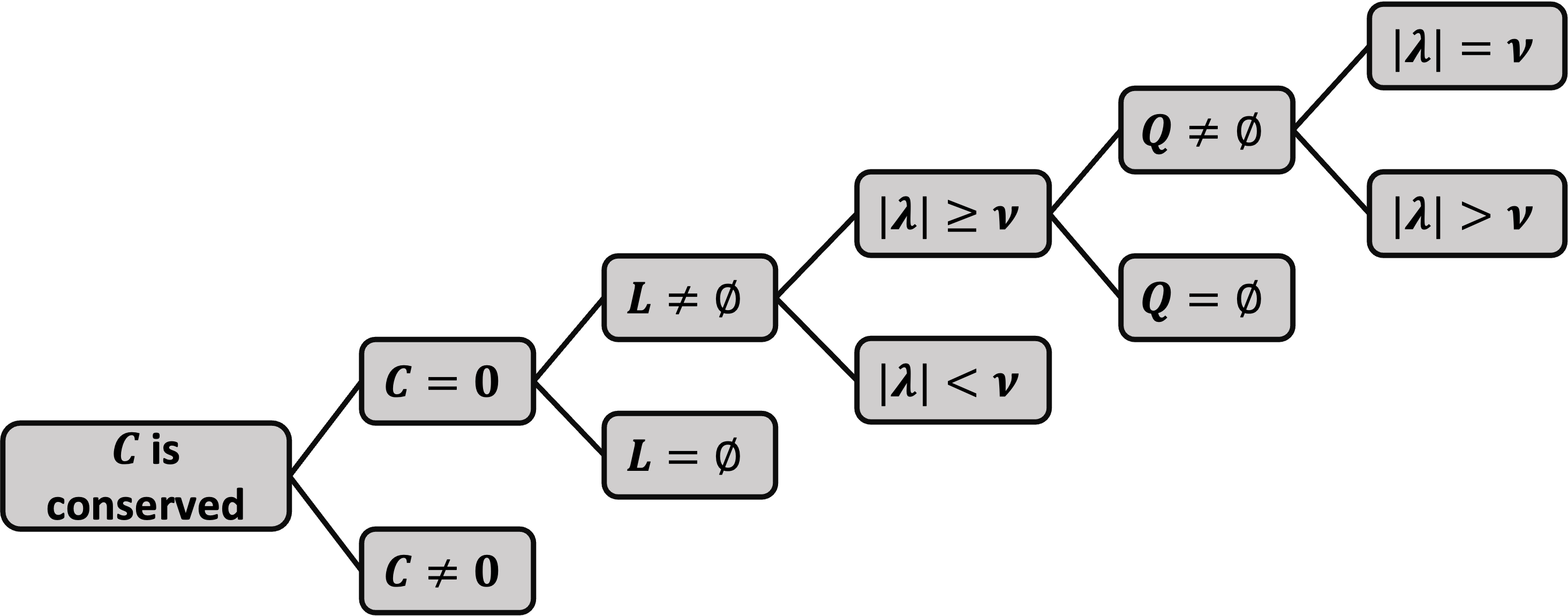
Figure 1: Case Study Analysis in the Proof of Theorem 1 in Sussmann (1995)

Throughout the case study analysis, four cases employed the cycle argument. First is when $C=0$, $L\neq\emptyset$, and $\|\lambda\|<\nu$, where it was concluded that $\gamma$ is a circular arc of length $<2\pi$. Without the cycle argument, $\gamma$ is a circular arc without such length bounds. Second is when $C=0$, $L\neq\emptyset$, $\|\lambda\|\geq\nu$, and $Q=\emptyset$. Similar to the previous case, without the cycle argument, it follows that $\gamma$ is a circular arc without length bounds. Third is when $C=0$, $L\neq\emptyset$, $\|\lambda\|\geq\nu$, $Q\neq\emptyset$, and $\|\lambda\|=\nu$. Here, $\hat{\mathcal{J}}$ was proven to be empty because any $J\in\hat{\mathcal{J}}$ must correspond to a cycle. However, detaching the cycle and attaching it to any point on the trajectory does not alter the overall length, as well as the initial and terminal positions and directions. As a result, any cycles corresponding to $J\in\hat{\mathcal{J}}$ can be attached to either the initial or terminal points. This modification either results in an auxiliary trajectory that violates the PMP conditions, or simplifies the overall trajectory to CSC or its subsegments. Such statement is available due to the subtlety between the statements of Theorem 2 and 6. Theorem 2 tells that every trajectory reaching the boundary of the reachability set must satisfy the maximum principle, while Theorem 6 only states that for every boundary points of the reachability set, there exists a trajectory belonging to the stated classes that reaches the point. Last is when $C=0$, $L\neq\emptyset$, $\|\lambda\|\geq\nu$, $Q\neq\emptyset$, and $\|\lambda\|>\nu$. The most definitive conclusion that can be made solely based on PMP conditions in this case is as follows: $\gamma$ is a planar curve constitutes a finite concatenation of circular arcs, all with the same length $2\alpha\geq\pi$, except possibly the first and last ones, with lengths $\leq 2\alpha$. Thus, the planar argument of this theorem is proved here for the minimum time case. Let us further denote such classes by multiple Cs. Further conclusion that the minimum time paths must be CC or CCC was derived from the geometric arguments pertaining to planar situations, proved in Dubins (1957). Hence, it remains to show that the curves of multiple Cs with more than three components can be disregarded for construction of the boundary of reachability sets. However, we will postpone this proof until the conclusion of our discussion on the maximum time problem. The conclusion so far is that the endpoints of the PMP sense solutions of minimum time problem can be reached by H, CSC, multiple Cs, or their subsegments.

To solve the maximum time problem, it suffices to only change the sign of the variable $\nu$ to be nonpositive. Then, the developments until Eq. (27) of Sussmann (1995) are identical. The subsequent part is the case study of $C\neq 0$ and $C=0$. When $C\neq 0$, Eq. (26) of Sussmann (1995) can be cast into Eq. (13) by means of elementary calculations, where $\zeta=\frac{2\nu}{\sqrt{|C|}}\leq 0$. The only difference between Eq. (13) of our paper and Eq. (6) in Sussmann (1995) is the nonpositivity of $\zeta$ instead of nonnegativity. Hence, the existence theory for the solutions of ODE can be applied analogously. Resultingly, the first case when $C\neq 0$ reduces to a similar result with the minimum time solution, an helicoidal arc.

When $C=0$, $\alpha$ is characterized by $A\cos\alpha=-\nu$ where $\nu\leq 0$. Then from the sign of $\nu$, we see that $2\alpha\leq\pi$. For the first subcase when $L=\emptyset$, $\gamma$ is a straight line by analogous arguments in Sussmann (1995). When $L\neq\emptyset$, nonpositivity of $\nu$ indicates that it suffices to only consider the case of $\|\lambda\|\geq\nu$. If $Q=\emptyset$, then $W$ is nonvanishing and hence $\gamma$ is a circular arc. It is worth emphasizing that the absence of the cycle argument allows such arc to have length $\geq 2\pi$. If $Q\neq\emptyset$, the cases $\|\lambda\|>\nu$ and $\|\lambda\|=\nu$ are considered separately. When $\|\lambda\|>\nu$, analogous steps imply that $\gamma$ is of multiple Cs, but with lengths of the middle arcs equal to $2\alpha\leq\pi$. Again, analogous approach used in the minimum time problem case can be applied to prove the planar argument here. If $\|\lambda\|=\nu$, nonpositivity of $\nu$ implies that $\lambda=\boldsymbol{0}$ and $\nu=0$. Consequently, $\varphi\equiv 0$ by definition. Then the second equation in Eq. (15) of Sussmann (1995) implies that $W\equiv 0$, which contradicts the first inequality, $\|\lambda\|+\|W\|>0$. Therefore, there exists no nontrivial solution in this case. The conclusion so far is that the PMP sense solutions of maximum time problem are of H, S, or multiple Cs.

Now, suppose $\gamma$ is of multiple Cs with more than three segments, denoted by $C_{1}C_{2}C_{3}\dots C_{n-1}C_{n}$. Then $C_{2}$ and $C_{3}$ have same lengths. Then it follows that the sum of the lengths of $C_{1}$ and $C_{3}$ are larger than $C_{2}$. Consequently, if the middle arcs are of length $<2\pi$, Lemma 2 of Patsko et al. (2003) indicates that there exists an auxiliary trajectory that violates the PMP. Therefore, the endpoints of such trajectories cannot lie on the boundary of the reachability set. If the middle arcs are of lengths $\geq 2\pi$, consist of full cycles, then the circle $C_{2}$ can be attached to an arbitrary point on the circle $C_{3}$ while maintaining the initial and terminal positions and directions, and the overall length of the trajectory. This auxiliary trajectory violates the PMP, that the middle arcs must have same lengths. Analogous argument was used to prove Lemma 3 in Patsko et al. (2003). This completes the proof. ∎

3.1.1 Reachability Set Without Considering Terminal Direction

In this subsection, we present the construction method of the reachability set boundary without considering the terminal direction. The results coincide with the 2D case studied in Cockayne and Hall (1975).

Theorem 13.

Any boundary point of the reachability set without consideration of terminal directions can be reached by the curves belonging to the following classes: CS, CC, or their subsegments. Moreover, curves of CC required to reach the boundary points are limited to planar curves.

Proof. Consideration of the reachability only on $x$ but not on $y$ implies that $\nabla\Phi=[(\cdot),\;(\cdot),\;(\cdot),\;0,\;0,\;0]^{T}$ in $\textbf{P0}_{\Phi}$, where $(\cdot)$ are unspecified values. The components corresponding to $y$ are considered zero, as the cost dependency on $y$, or the terminal direction is not considered. Then from the transversality condition of $\textbf{P0}_{\Phi}$, it follows $\mu(b)=\boldsymbol{0}$. Consequently, $W=0$ at $b$ by definition, and hence $C=\psi\|W\|=0$. Therefore, H can be disregarded when constructing the boundary of the reachability set. It remains to show that CSC or CCC curves can be reduced to CS or CC.

When $C=0$, a $C_{1}C_{2}C_{3}$ curve can be a PMP sense solution in two cases. First is when $L\neq\emptyset$, $\|\lambda\|>\nu$, and $Q\neq\emptyset$. Consequently, $W=0$ at $b$ further implies $b\notin L$ and $b\in Q$. Since $Q$ is a finite set as proved in Sussmann (1995), $C_{2}$ and $C_{3}$ have same length $2\alpha$. Then Lemma 2 of Patsko et al. (2003) can be applied to construct an auxiliary trajectory, as in the previous proof of Theorem 12 in our paper. Second is when $L\neq\emptyset$, $\|\lambda\|=\nu$, and $Q\neq\emptyset$. In this case, for the overall trajectory to be a $C_{1}C_{2}C_{3}$ curve, $\hat{\mathcal{J}}$ must be nonempty and $\mathcal{K}$ must consist of isolated points. Then from $\|\lambda\|=\nu$, it follows $\cos\alpha=-\frac{\nu}{\|\lambda\|}=-1$ which implies that $C_{2}$ corresponding to $J\in\hat{\mathcal{J}}$ must have length of a cycle, $2\alpha=2\pi$, or multiple cycles. As a result, the winding direction of $C_{2}$ can be reversed without altering the initial and terminal positions and directions, as well as maintaining the overall length of the trajectory. Then the overall curve is reduced to C.

Similarly when $C=0$, a CSC curve can be a PMP sense solution only if $L\neq\emptyset$, $\|\lambda\|=\nu$, and $Q\neq\emptyset$. Then similar to the previous case of CCC, the last C corresponding to the interval $J\in\tilde{\mathcal{J}}$ must have length $2\alpha=2\pi$ of a cycle, or of multiple cycles. Consequently, the last C can be attached to the first C while preserving the initial and terminal positions and directions, and the overall length of the trajectory. Then the overall curve is reduced to CS. ∎

4 Conclusion

This paper introduces the concept of equivalence relation on set of optimal control problems based on the Pontryagin maximum principle. Utilizing this concept, it is proved that the boundary points of the reachability set can be accessed by time optimal solutions. As a byproduct, the construction method of reachability sets for 3D curvature bounded paths are presented as well. The results generalize the existing literatures on 2D. As the foundational studies on identifying the reachability set of planar curves did, such generalization into 3D curves is anticipated to enable various advancements in guidance laws and mission planning methods. We would like to extend our gratitude to Nearthlab for insights and expertise during the review process of our paper.

References

- (1)
- Althoff (2010) Althoff, M. (2010). Reachability Analysis and its Application to the Safety Assessment of Autonomous Cars. PhD thesis.
- Bae et al. (2024) Bae, J., Ji Hoon Bai, Byung-Yoon Lee and Jun-Yong Lee (2024). ‘Constraint-aware mesh refinement method by reachability set envelope of curvature bounded paths’.
- Buzikov and Galyaev (2021) Buzikov, M. E. and A. A. Galyaev (2021). ‘Time-optimal interception of a moving target by a dubins car’. Autom. Remote Control 82(5), 745–758.
- Buzikov and Galyaev (2022) Buzikov, M. E. and Andrey A. Galyaev (2022). ‘Minimum-time lateral interception of a moving target by a dubins car’. Automatica 135, 109968.
- Chen et al. (2023) Chen, Z., Kun Wang and Heng Shi (2023). ‘Elongation of curvature-bounded path’. Automatica 151, 110936.
- Cockayne and Hall (1975) Cockayne, E. J. and G. W. C. Hall (1975). ‘Plane motion of a particle subject to curvature constraints’. SIAM Journal on Control 13(1), 197–220.
- Dubins (1957) Dubins, L. E. (1957). ‘On curves of minimal length with a constraint on average curvature, and with prescribed initial and terminal positions and tangents’. American Journal of Mathematics 79(3), 497–516.
- Hartl et al. (1995) Hartl, R. F., Suresh P. Sethi and Raymond G. Vickson (1995). ‘A survey of the maximum principles for optimal control problems with state constraints’. SIAM Review 37(2), 181–218.
- Lee and Markus (1967) Lee, E. B. and Lawrence Markus (1967). Foundations of optimal control theory.
- Lewis (2006) Lewis, A. D. (2006). ‘The maximum principle of pontryagin in control and in optimal control’. Handouts for the course taught at the Universitat Politecnica de Catalunya.
- Lin and Saripalli (2014) Lin, Y. and Srikanth Saripalli (2014). Path planning using 3d dubins curve for unmanned aerial vehicles. In ‘2014 International Conference on Unmanned Aircraft Systems (ICUAS)’. pp. 296–304.
- Lygeros (2004) Lygeros, J. (2004). ‘On reachability and minimum cost optimal control’. Automatica 40(6), 917–927.
- McGregor et al. (1999) McGregor, C., David Glasser and Diane Hildebrandt (1999). ‘The attainable region and pontryagin’s maximum principle’. Industrial & Engineering Chemistry Research 38, 652–659.
- Patsko and Fedotov (2020) Patsko, V. S. and A. A. Fedotov (2020). ‘Analytic description of a reachable set for the dubins car’. Trudy Inst. Mat. i Mekh. UrO RAN 26(1), 182–197.
- Patsko et al. (2003) Patsko, V., S.G. Pyatko and Andrey Fedotov (2003). ‘Three-dimensional reachability set for a nonlinear control system’. Journal of Computer and Systems Sciences International.
- Scibilia et al. (2012) Scibilia, F., Ulrik Jørgensen and Roger Skjetne (2012). ‘Auv guidance system for dynamic trajectory generation’. IFAC Proceedings Volumes 45(5), 198–203. 3rd IFAC Workshop on Navigation, Guidance and Control of Underwater Vehicles.
- Sussmann (1995) Sussmann, H. (1995). ‘Shortest 3-dimensional paths with a prescribed curvature bound’. Proceedings of the IEEE Conference on Decision and Control 4, 3306–3312. Proceedings of the 1995 34th IEEE Conference on Decision and Control. Part 1 (of 4) ; Conference date: 13-12-1995 Through 15-12-1995.
- Wong and Korsak (1974) Wong, P. J. and Andrew J. Korsak (1974). ‘Reachable sets for tracking’. Oper. Res. 22(3), 497–509.
- Zheng et al. (2021) Zheng, Y., Zheng Chen, Xueming Shao and Wenjie Zhao (2021). ‘Time-optimal guidance for intercepting moving targets by dubins vehicles’. Automatica 128, 109557.