Conditional Wasserstein Distances with Applications in Bayesian OT Flow Matching

Jannis Chemseddine, Paul Hagemann, Christian Wald, Gabriele Steidl
Abstract

In inverse problems, many conditional generative models approximate the posterior measure by minimizing a distance between the joint measure and its learned approximation. While this approach also controls the distance between the posterior measures in the case of the Kullback–Leibler divergence, this is in general not hold true for the Wasserstein distance. In this paper, we introduce a conditional Wasserstein distance via a set of restricted couplings that equals the expected Wasserstein distance of the posteriors. Interestingly, the dual formulation of the conditional Wasserstein-1 flow resembles losses in the conditional Wasserstein GAN literature in a quite natural way. We derive theoretical properties of the conditional Wasserstein distance, characterize the corresponding geodesics and velocity fields as well as the flow ODEs. Subsequently, we propose to approximate the velocity fields by relaxing the conditional Wasserstein distance. Based on this, we propose an extension of OT Flow Matching for solving Bayesian inverse problems and demonstrate its numerical advantages on an inverse problem and class-conditional image generation.

1 Introduction

Many sampling algorithms for the posterior $P_{X|Y=y}$ in Bayesian inverse problems

$$Y=f(X)+\Xi$$ (1)

with a forward operator $f:\mathbb{X}\to\mathbb{Y}$, and a noise model $\Xi$, perform learning on some joint measures. This means, given some observations $y$ of $Y$, a probability measure $P_{Y,G_{\theta}}$ is learned, where $G_{\theta}$ also depends on $y$. Most approaches minimize (or upper bound) some loss of the form

$$L(\theta)=D(P_{Y,X},P_{Y,G_{\theta}}),$$

where $D$ denotes a suitable distance on the space of probability measures. For instance, this is done in the framework of conditional (stochastic) normalizing flows [7, 26, 25, 54], conditional GANs [40] or conditional gradient flows for the Wasserstein metric [18, 24]. Note that the robustness of such conditional generative models was shown under the assumption that the expected error to the posterior $E_{Y}\left[W_{1}(P_{X|Y=y},P_{Z|Y=y})\right]$ is small in [3], which shows that it is important to relate this quantity to the approximation of the joint measures.

In [31], the authors investigated the relation between the joint measures $D(P_{Y,Z},P_{Y,X})$ and its relation to the expected error between the posteriors $E_{Y}\left[D(P_{Z|Y=y},P_{X|Y=y})\right].$ For the Kullback–Leibler divergence $D=\text{KL}$, it follows by the chain rule [16, Theorem 2.5.3] that

$$E_{Y}\left[\mathrm{KL}(P_{X|Y=y},P_{Z|Y=y})\right]=\mathrm{KL}(P_{Y,X},P_{Y,Z}).$$

Such results are important as they show that it is possible to approximate the posterior via the joint distribution. Unfortunately, we have for the Wasserstein-1 distance that in general only

$$W_{1}(P_{Y,X},P_{Y,Z})\leq\mathbb{E}_{y\sim P_{Y}}\left[W_{1}(P_{X|Y=y},P_{Z|Y=y})\right]$$ (2)

holds true, in contrast to the equality claim in [31, Theorem 2]. A simple counterexample is given in Appendix A. Intuitively, strict inequality can arise when the optimal transport (OT) plan needs to transport mass in the $Y$-component. This is the motivation for considering only plans that do not have mass transport in the $Y$-component. This leads us to the definition of conditional Wasserstein distances $W_{p,Y}$, where admissible transport plans are restricted to the set $\Gamma_{Y}^{4}=\Gamma_{Y}^{4}(P_{Y,X},P_{Y,Z})$ of 4-plans $\alpha$ fulfilling in addition $(\pi^{1,3})_{\sharp}\alpha=\Delta_{\sharp}P_{Y}$, where $\Delta(y)=(y,y)$ is the diagonal map:

$\displaystyle W_{p,Y}^{p}\coloneqq\underset{\alpha\in\Gamma_{Y}^{4}}{\mathsf{inf}}\int\|(y_{1},x_{1})-(y_{2},x_{2})\|^{p}\,\mathrm{d}\alpha$

Inspired by [31], we show that this conditional Wasserstein distance indeed fulfills

$$W_{p,Y}^{p}(P_{Y,X},P_{Y,Z})=\mathbb{E}_{y\sim P_{Y}}\left[W_{p}^{p}(P_{X|Y=y},P_{Z|Y=y})\right].$$

Further, we prove results on gradient flows [6] with respect to our conditional Wasserstein distance: we show the connections to the continuity equation, verify that there exists a velocity field with no mass transport in $Y$-direction and recover a corresponding ODE formulation. Indeed, this conditional Wasserstein distance can be used to explain a numerical observation made by [18, 24], namely that rescaling the $Y$-component leads to velocity fields with no mass transport in Y-direction in the limit. Using these ideas, we propose to relax the conditional Wasserstein distance to allow "small amounts" of mass transport in $Y$-direction.

Then, we use our insights to design efficient posterior sampling algorithms. By leveraging recent ideas of flow matching [35, 36], we design Bayesian OT flow matching. Note that the recent approaches of [55, 53] do not respect the OT in $X$-direction as they always choose the diagonal coupling. This leads to awkward situations, where the optimal $Y$-diagonal coupling is not recovered even between Gaussians, see Example 9. We use our proposed Bayesian OT flow matching and verify its advantages on a Gaussian mixture toy problem and on class conditional image generation on the CIFAR10 dataset.

Contributions

  • We introduce conditional Wasserstein distances and highlight their relevance to conditional Wasserstein GANs in inverse problems.

  • We derive theoretical properties of the conditional Wasserstein distance and establish geodesics in this conditional Wasserstein space, with velocity plans having no transport in $Y$-direction.

  • We show that the conditional Wasserstein distance can be used in conditional generative approaches and demonstrate the advantages on MNIST particle flows [24, 4]. We propose a version of OT flow matching [50, 44] for inverse problems which uses a relaxed version of our conditional Wasserstein distance, and show that it overcomes obstacles from previous flow matching versions for inverse problems [53].

Related work

Our work is in the intersection of conditional generative modelling [1, 7, 40] and (computational) OT [43, 51]. The recent work [22, Theorem 2] derives an inequality based on restricting the admissible couplings in the their OT formulation to so-called conditional sub-couplings. Note that their reformulation is only a restatement of the expected value, but does not relate it to the joint distributions. Those authors also look for geodesics in the Wasserstein space, but pursue a different approach. While we relate it to the velocity fields in gradient flows, they pursue an autoencoder/GAN idea.

The closest work, which appeared after our first version of this paper, is [29]. Unfortunately, we became aware of those paper when our paper was close to its finish. Here the authors define the conditional optimal transport problem and calculate its dual. Their work is more focused on the infinite dimensional setting, whereas we consider the velocity fields needed for the flow matching application.

In the OT literature, there has been a collection of class conditional OT distances used in domain adaption [41, 45]. In particular, conditional OT as in [48] is relevant as they consider OT plans for each condition $y$ minimizing $\mathbb{E}_{y}[W_{1}(P_{X|Y=y},G(\cdot,y)_{\#}P_{Z})]$. However they relax their problem using a KL divergence. The papers on Wasserstein gradient flows [5, 23] investigate conditional Wasserstein distances from a different point of view for defining the so-called geometric tangent space of the 2-Wasserstein space. Geometric tangent spaces play a crucial role in Wasserstein flows of maximum mean discrepancies with Riesz kernels in [27] and their neural variants in [4]. In [24, Remark 7], an inequality between the joint Wasserstein and the expected value over the conditionals is derived, where the result requires compactly supported measures and certain regularity of the associated posterior densities. In [12]. the supervised training of conditional Monge maps is proposed, for which the authors solved the dual problem using convex neural networks. The authors of [37] also considers an amortized objective between the conditional distributions and propose a relaxation, which only needs samples from the joint distribution involving maximum mean discrepancies. Numerically, we first verify our theoretical statements based on particle flows, which were also used in [4, 24]. Further, we apply our framework to solve inverse problems using Bayesian flow matching [53, 55] and OT flow matching [35, 36, 50, 44].

This paper is an extension of our first ArXiv version [13] on conditional Wasserstein distances with more focus on gradient flows and flow matching.

Outline of the paper

In Section 2, we recall preliminaries from OT. Then, in Section 3, we introduce conditional Wasserstein distances of joint probability measures, and show their relation to the expectation over the Wasserstein distance of the conditional probabilities. Moreover, we highlight the connection to work on geometric tangent spaces. In Section 4, we calculate the dual of our conditional Wasserstein-1 distance and show how a loss function used in the conditional Wasserstein GAN literature arises in a natural way. In Section 5, we deal with geodesics with respect to the conditional Wasserstein distance, prove properties of the corresponding velocity fields, showing that they vanish in the $Y$-component, and show existence for flow ODEs. We propose a relaxation of the conditional Wasserstein distance which appears to be useful for numerical computations in Section 6. We combine our findings with OT flow matching to get Bayesian flow matching in Section 6. Finally, in Section 8, we present numerical results: we verify a convergence result using particle flows to MNIST, and demonstrate the advantages of our Bayesian OT flow matching procedure on a Gausian mixture model toy example and on CIFAR10 class-conditional image generation. All proofs are postponed to the appendix.

2 Preliminaries

Throughout this paper, we will use the following notation. These are basics from from optimal transport theory and can be found in [51]. By $\mathcal{P}(\mathbb{X})$, we denote the set of probability measures on $\mathbb{X}\subseteq\mathbb{R}^{n}$ and by $\mathcal{P}_{p}(\mathbb{X})$, $p\in[1,\infty)$ the subset of measures with finite $p$-th moments. For $\mu\in\mathcal{P}(\mathbb{X})$ and a measurable function $F:\mathbb{X}\to\mathbb{Y}$, we define the the push forward measure by $F_{\sharp}\mu=F\circ\mu^{-1}$. For a product space $\prod_{i=1}^{K}\mathbb{X}_{i}$, we denote the projection onto the $i_{1},\ldots,i_{k}$-th component by $\pi^{i_{1},\ldots,i_{k}}$. The Wasserstein-$p$ metric [51] on $\mathcal{P}_{p}(\mathbb{X})$ is given by

$\displaystyle W_{p}(\mu,\nu)$ $\displaystyle\coloneqq\Big{(}\min_{\gamma\in\Gamma}\int_{\mathbb{X}^{2}}\|x-y\|^{p}\,\text{d}\gamma(x,y)\Big{)}^{\frac{1}{p}}$ (3)
$\displaystyle=\Big{(}\min_{\gamma\in\Gamma}\mathbb{E}_{(x,y)\sim\gamma}\big{[}\|x-y\|^{p}\big{]}\Big{)}^{\frac{1}{p}}.$ (4)

where $\Gamma=\Gamma(\mu,\nu)$ denotes the set of all probability measures $\gamma\in\mathcal{P}(\mathbb{X}\times\mathbb{X})$ with marginals $\pi^{1}_{\sharp}\gamma=\mu$ and $\pi^{2}_{\sharp}\gamma=\nu$ and $\|\cdot\|$ is the Euclidean distance on $\mathbb{R}^{n}$, see [51]. If $\mu\in\mathcal{P}_{p}(\mathbb{X})$ is absolutely continuous, then, for $p\in(1,\infty)$, there exits a unique optimal transport map $T\in L^{p}_{\mu}(\mathbb{X},\mathbb{X})$, also known as Monge map, which solves

$$\min_{T\,\text{measurable}}\Big{\{}\int_{\mathbb{X}}\|x-T(x)\|^{p}\,\text{d}\mu(x)\quad\text{such that}\quad T_{\sharp}\mu=\nu\Big{\}}.$$

Further, this optimal map is related to the optimal transport plan $\gamma$ in (3) by $\gamma=(\mathrm{Id},T)_{\sharp}\mu,$ see [51]. The same holds true for empirical measures with the same number of points, see [43, Proposition 2.1]. In this paper, we ask for relations between joint and posterior probabilities: for random variables $X,Z\in B\subseteq\mathbb{R}^{m}$ and $Y\in A\subseteq\mathbb{R}^{d}$, we are interested in Wasserstein distances between $P_{Y,X},P_{Y.Z}\in\mathcal{P}_{p}(A\times B)$ and $P_{X|Y=y},P_{Z|Y=y}\in\mathcal{P}_{p}(B)$. Since $\pi^{1}_{\sharp}P_{Y,X}=P_{Y}$ as well as $\pi^{1}_{\sharp}P_{Y,Z}=P_{Y}$, we see that the joint probabilities belong indeed to the subset

$$\mathcal{P}_{p,Y}(A\times B)\coloneqq\{\gamma\in\mathcal{P}_{p}(A\times B):\pi^{1}_{\sharp}\gamma=P_{Y}\}.$$ (5)

For $p=2$, this set was considered as set of velocity plans at $P_{Y}$ in [6, Sect. 12.4] and [23, Sect. 4]. It is the basis for defining the so-called geometric tangent space of $\mathcal{P}_{2}(\mathbb{R}^{d})$ which was used, e.g. in [27, 4] for handling (neural) Wasserstein gradient flows of maximum mean discrepancies.

We will frequently apply the disintegration formula [6, Theorem 5.3.1] which says that for a measure $\gamma\in\mathcal{P}(A\times B)$ with $\pi^{1}_{\sharp}\gamma=\mu\in\mathcal{P}(A)$, there exists a $\mu$-a.e. uniquely determined Borel family of probability measures $(\gamma_{y})_{y\in A}$ such that

$$\int_{A\times B}f(y,x)\,\mathrm{d}\gamma(y,x)=\int_{A}\int_{B}f(y,x)\,\mathrm{d}\gamma_{y}(x)\mathrm{d}\mu(y)$$ (6)

for any Borel measurable map $f:A\times B\to[0,+\infty]$. In particular, for $\gamma=P_{Y,X}\in\mathcal{P}(A\times B)$, the disintegration formula reads as

$$\int_{A\times B}f(y,x)\,\mathrm{d}P_{Y,X}(y,x)=\int_{A}\int_{B}f(y,x)\,\mathrm{d}P_{X|Y}(x)\mathrm{d}P_{Y}(y).$$ (7)

3 Conditional Wasserstein distance

We have already seen that in general we can only expect inequality in (2). Towards equality, we introduce a conditional Wasserstein distance which allows only couplings which leave the $Y$-component invariant. To this end, we introduce the set of special 4-plans

$$\Gamma_{Y}^{4}=\Gamma_{Y}^{4}(P_{Y,X},P_{Y,Z})\coloneqq\Big{\{}\alpha\in\Gamma(P_{Y,X},P_{Y,Z}):\pi^{1,3}_{\sharp}\alpha=\Delta_{\sharp}P_{Y}\Big{\}},$$ (8)

where $\Delta:A\to A^{2}$, $y\mapsto(y,y)$ is the diagonal map. Note that $\Delta^{-1}(y_{1},y_{2})=\emptyset$ if $y_{1}\not=y_{2}$ and $\Delta^{-1}(y_{1},y_{2})=y$ if $y_{1}=y_{2}=y$. Then, we define the conditional Wasserstein-$p$ distance, $p\in[1,\infty)$ by

$\displaystyle W_{p,Y}(P_{Y,X},P_{Y,Z})\coloneqq\Big{(}\inf_{\alpha\in\Gamma_{Y}^{4}}\int_{(A\times B)^{2}}\|(y_{1},x_{1})-(y_{2},x_{2})\|^{p}\,\mathrm{d}\alpha\Big{)}^{\frac{1}{p}}.$ (9)

Indeed we will see in Corollary 2 that this is a metric on $\mathcal{P}_{p,Y}(A\times B)$.

In terms of Monge maps, this means that we are considering functions $(\mathrm{Id},T(y,\cdot)):(y,x)\mapsto(y,T(y,x))$, where $T:\mathbb{R}^{d}\times\mathbb{R}^{m}\to\mathbb{R}^{m}$ and $(\mathrm{Id},T(y,\cdot))_{\#}P_{Y,X}=P_{Y,Z}$. The following proposition gives the desired equivalence of the form (2). The proof is given in Appendix B.

Proposition 1.

The following relations holds true.

  • i)

    The conditional Wasserstein-$p$ distance (9) fulfills

    $\displaystyle W_{p,Y}^{p}(P_{Y,X},P_{Y,Z})=\mathbb{E}_{Y}\big{[}W_{p}^{p}(P_{X|Y=y},P_{Z|Y=y})\big{]}.$ (10)
  • ii)

    Let $\alpha\in\Gamma_{p,Y}^{4}$ is an optimal plan in (9) with disintegration $\alpha_{y_{1},y_{2}}$ with respect to $\pi^{1,3}_{\sharp}\alpha$. Then $\alpha_{y,y}\in\mathcal{P}(\mathbb{R}^{2m})$ is an optimal plan for $W_{p}(P_{X|Y=y},P_{Z|Y=y})$ for $P_{Y}$-a.e. $y\in A$.

  • iii)

    There exists a collection of optimal plans $\alpha_{y}\in\Gamma(P_{X|Y=y},P_{Z|Y=y})$, $y\in A$ for

    $W_{p}(P_{X|Y=y},P_{Z|Y=y})$ such that

    $$\alpha\coloneqq\int_{A}\mathrm{d}\delta_{y_{1}}(y_{2})\,\mathrm{d}\alpha_{y_{1}}(x_{1},x_{2})\mathrm{d}P_{Y}(y_{1})$$ (11)

    is a well-defined coupling in $\Gamma_{Y}^{4}$ which is optimal in (9).

For $p=2$, it was shown in [6, Sect. 12.4] and [23, Sect. 4] that the square root of the right-hand side in (7) is a metric on $\mathcal{P}_{2,Y}(A\times B)$. The proof can be generalized in a straightforward way for $p\in[1,\infty)$. Thus, by Proposition 1, we have the following corollary.

Corollary 2.

The conditional Wasserstein distance $W_{p,Y}$ is a metric on $\mathcal{P}_{p,Y}(A\times B)$.

Interestingly, for $p=2$, there was also given an equivalent definition by [23] of $\mathcal{W}_{p,Y}$, namely

$$\mathcal{W}_{p,Y}(P_{Y,X},P_{Y,Z})\coloneqq\underset{\beta\in\Gamma^{3}_{Y}(P_{Y,X},P_{Y,Z})}{\inf}\ \Big{(}\int_{A\times B^{2}}\|x_{1}-x_{2}\|^{p}\,\mathrm{d}\beta(y,x_{1},x_{3})\Big{)}^{\frac{1}{p}}$$ (12)

with the set of 3-plans

$$\Gamma^{3}_{Y}(P_{Y,X},P_{Y,Z})\coloneqq\{\beta\in\mathcal{P}_{p}(A\times B^{2}):\pi^{1,2}_{\sharp}\beta=P_{Y,X},\pi^{1,3}_{\sharp}\beta=P_{Y,Z}\}.$$

The relation between the admissible 3-plans and 4-plans is given in the following proposition which proof can be found in the appendix.

Proposition 3.

The map $\pi^{1,2,4}_{\sharp}:\Gamma_{Y}^{4}(P_{Y,X},P_{Y,Z})\to\Gamma_{Y}^{3}(P_{Y,X},P_{Y,Z})$ is a bijection and for every $\alpha\in\Gamma_{Y}^{4}(P_{Y,X},P_{Y,Z})$ it holds

$\displaystyle\int_{(A\times B)^{2}}\|(y_{1},x_{1})-(y_{2},x_{2})\|^{p}\,\mathrm{d}\alpha=\int_{A\times B^{2}}\|x_{1}-x_{2}\|^{p}\,\mathrm{d}\pi^{1,2,4}_{\sharp}\alpha.$

4 Dual formulation of $W_{1,Y}$ and relation to GAN loss

Interestingly, the conditional Wasserstein-1 distance recovers loss functions in the conditional Wasserstein GAN literature [1, 31, 38]. Wasserstein GANs [8] aim to sample from a target distribution $P_{X}$ based on a simpler distribution $P_{Z}$, a generator $G=G_{\theta}$ is learned such that the Wasserstein-1 distance in its dual formulation

$\displaystyle W_{1}(P_{X},G_{\#}P_{Z})=\max_{f\in\text{Lip}_{1}}\left\{\mathbb{E}_{X}[f]-\mathbb{E}_{Z}\big{[}f\circ G\big{]}\right\}$

is minimized, where $\text{Lip}_{1}$ denotes the set of 1-Lipschitz continuous functions. At the same time, a discriminator $f=f_{\omega}$ is learned such that the final Wasserstein GAN learning problem becomes

$\displaystyle\min_{\theta}\max_{\omega}\left\{\mathbb{E}_{X}[f]-\mathbb{E}_{Z}[f\circ G]\right\}\quad\text{subject to}\quad f\in\text{Lip}_{1}.$

Usually, the the 1-Lipschitz condition is enforced via so-called weight-clipping [8].

In [1], this approach was generalized to inverse problems. Assume that $A\subset\mathbb{R}^{d}$ and $B\subset\mathbb{R}^{m}$ are compact sets throughout this section. For given $y\in A$, an optimal $h(y,\cdot)\in\text{Lip}_{1}$ is found in

$\displaystyle W_{1}(P_{X|Y=y},G(y,\cdot)_{\#}P_{Z})=\max_{h(y,\cdot)\in\text{Lip}_{1}}\left\{\mathbb{E}_{X|Y=y}[h(y,x)]-\mathbb{E}_{Z}\big{[}h(y,G(y,\cdot))\big{]}\right\}.$

Now the authors take the expectation value on both sides and exchange expectation and maximum to get, together with (7), the relation

$\displaystyle\mathbb{E}_{Y}[W_{1}(P_{X|Y=y},G(y,\cdot)_{\#}P_{Z}]=\max_{h}\left\{\mathbb{E}_{Y,X}[h]-\mathbb{E}_{Y,Z}[h(y,G(y,\cdot)]\right\},$ (13)

where the maximum is taken over functions $h$ which are Lipschitz-1 continuous in the second variable. However, exchanging maximum and expectation value requires that $(y,x)\mapsto h(y,x)$ is measurable which is not always the case. This ,,gap” was fixed under stronger assumptions, e.g. on the posterior, in [38].

In this section, we show that the dual formulation of the conditional Wasserstein distance $W_{1,Y}$ leads naturally to the desired loss on the right-hand side of (13) for an appropriate regular function set for $h$. More precisely, we have the following theorem which is proved in the appendix.

Theorem 4.

Let $A\subset\mathbb{R}^{d}$ and $B\subset\mathbb{R}^{m}$ be compact sets. Then it holds

$\displaystyle W_{1,Y}(P_{Y,X},P_{Y,Z})=\sup_{h\in\mathcal{F}}\left\{\mathbb{E}_{Y,X}[h]-\mathbb{E}_{Y,Z}[h(y,G(y,\cdot)]\right\},$

where $\mathcal{F}$ denotes the set of bounded, upper semi-continuous functions $h:A\times B\to\mathbb{R}$ satisfying $|h(y,x_{1})-h(y,x_{2})|\leq\|x_{1}-x_{2}\|$ for all $y\in A$ and all $x_{1},x_{2}\in B$.

5 Geodesics and velocity fields

In this section, we deal with geodesics and velocity fields in $\left(\mathcal{P}_{Y,2}(\mathbb{R}^{d}\times\mathbb{R}^{m}),W_{2,Y}\right)$. We restrict our attention to $p=2$ and $A=\mathbb{R}^{d}$, $B=\mathbb{R}^{m}$. Coming from inverse problems, we have considered probability measures $P_{X,Y}$ related to random variables $(Y,X)\in\mathbb{R}^{d}\times\mathbb{R}^{m}$. When switching to flows, it is more convenient to address equivalently just probability measures on $\mathbb{R}^{d}\times\mathbb{R}^{m}$.

Let us recall some results which can be found, e.g. in [6] for our setting. A curve $\mu\colon[0,1]\to\mathcal{P}_{2}(\mathbb{R}^{d}\times\mathbb{R}^{m})$ is called a geodesic if

$$W_{2}(\mu_{s},\mu_{t})=|s-t|W_{2}(\mu_{0},\mu_{1})\quad\text{for all}\quad s,t\in[0,1].$$ (14)

The Wasserstein space is geodesic, i.e. any two measures $\mu_{0},\mu_{1}\in\mathcal{P}_{2}(\mathbb{R}^{d}\times\mathbb{R}^{m})$ can be connected by a geodesic. Let $e_{t}:(\mathbb{R}^{d}\times\mathbb{R}^{m})^{2}\to\mathbb{R}^{n}\times\mathbb{R}^{m}$, $t\in[0,1]$ by defined by

$$e_{t}(y_{1},x_{1},y_{2},x_{2})\coloneqq\left((1-t)\pi^{1,2}+t\pi^{3,4}\right)(y_{1},x_{1},y_{2},x_{2})=(1-t)(y_{1},x_{1})+t(y_{2},x_{2}).$$ (15)

Any geodesic $\mu\colon[0,1]\to\mathcal{P}_{2}(\mathbb{R}^{d}\times\mathbb{R}^{m})$ connecting $\mu_{0},\mu_{1}\in\mathcal{P}_{2}(\mathbb{R}^{d}\times\mathbb{R}^{m})$ is determined by an optimal plan $\alpha\in\Gamma(\mu_{0},\mu_{1})$ in (3) via

$$\mu_{t}\coloneqq(e_{t})_{\sharp}\alpha,\quad t\in[0,1].$$ (16)

Conversely, any optimal plan $\alpha\in\Gamma(\mu_{0},\mu_{1})$ gives by (16) rise to a geodesic connecting $\mu_{0}$ and $\mu_{1}$. The following lemma considers curves defined by (16) which connect measures $\mu_{0},\mu_{1}\in\mathcal{P}_{2,Y}(\mathbb{R}^{d}\times\mathbb{R}^{m})$. Its proof is given in the appendix and is similar to [6, Theorem 7.2.2].

Lemma 5.

Let $\mu_{0},\mu_{1}\in\mathcal{P}_{2,Y}(\mathbb{R}^{d}\times\mathbb{R}^{m})$ and let $\alpha\in\Gamma_{Y}^{4}(\mu_{0},\mu_{1})$ be an optimal plan in (9). Then the following holds true.

  • i)

    The curve $\mu_{t}\coloneqq(e_{t})_{\sharp}\alpha$ is a geodesic in $(\mathcal{P}_{2,Y}(\mathbb{R}^{d}\times\mathbb{R}^{m}),W_{2,Y})$.

  • ii)

    The curve $(\mu_{t})_{y}:=(1-t)\pi^{1}+t\pi^{2})_{\sharp}\alpha_{y,y}$ is the disintegration of $\mu_{t}$ with respect to $P_{Y}$. Further, $(\mu_{t})_{y}$ is a geodesic in $(\mathcal{P}_{2}(\mathbb{R}^{m}),W_{2})$ for $P_{Y}$-a.e. $y\in\mathbb{R}^{d}$.

  • iii)

    $\mu_{t}$ is weakly continuous.

By the following proposition, the above geodesic $\mu_{t}$ has an associated vector field $v_{t}$ which satisfy a continuity equation. Moreover, informally speaking, the associated vector field $v_{t}$ does not transport any mass in the $y$-component. This is related to the observation in [18].

Proposition 6.

Let $\mu_{0},\mu_{1}\in\mathcal{P}_{2,Y}(\mathbb{R}^{d}\times\mathbb{R}^{m})$. Let $\alpha\in\Gamma_{Y}^{4}(\mu_{0},\mu_{1})$ be an optimal plan in (9) and $\mu_{t}=(e_{t})_{\sharp}\alpha$, $t\in[0,1]$. Then there exists a vector field $v_{t}\in L^{2}_{\mu_{t}}(\mathbb{R}^{d}\times\mathbb{R}^{m},\mathbb{R}^{d}\times\mathbb{R}^{m})$ such that the following relations are fulfilled:

  • i)

    $(e_{t})_{\sharp}\left((y_{2},x_{2})-(y_{1},x_{1})\right)\alpha)=v_{t}\mu_{t}$,

  • ii)

    $\|v_{t}\|_{L^{2}_{\mu_{t}}}\leq W_{2,Y}(\mu_{0},\mu_{1})$,

  • iii)

    for $j\leq d$, we have $(v_{t})_{j}=0$ $\mu_{t}$-a.e.,

  • iv)

    $\mu_{t},v_{t}$ fulfill the continuity equation

    $$\partial_{t}\mu_{t}+\nabla\cdot(v_{t}\mu_{t})=0$$

    in a distribultional sense, i.e. we have for all $\varphi\in C^{\infty}_{c}(\mathbb{R}^{d}\times\mathbb{R}^{m})$ that

    $\displaystyle\frac{\mathrm{d}}{\mathrm{d}t}\int_{\mathbb{R}^{d}\times\mathbb{R}^{m}}\varphi\,\mathrm{d}\mu_{t}=\int_{\mathbb{R}^{d}\times\mathbb{R}^{m}}\langle\nabla\phi,v_{t}\rangle\,\mathrm{d}\mu_{t}.$ (17)

The proof is given in Appendix D and parts $i),ii),iv)$ are adapted from the proofs of [5, Theorem 17.2, Lemma 17.3.]

Furthermore, since by Lemma 5 iii), a geodesic induced by an optimal $W_{2,Y}$ plan is weakly continuous, we obtain the following proposition from [6, Proposition 8.1.8] which is needed in the numerical section.

Proposition 7.

Let $\mu_{0},\mu_{1}\in\mathcal{P}_{2,Y}(\mathbb{R}^{d}\times\mathbb{R}^{m})$. Let $\alpha\in\Gamma_{Y}^{4}(\mu_{0},\mu_{1})$ be an optimal plan in (9) and $\mu_{t}=(e_{t})_{\sharp}\alpha$, $t\in[0,1]$. Assume that the corresponding Borel vector field $v_{t}$ from Proposition 6 fulfills

$\displaystyle\int_{0}^{1}\left(\sup_{B}(\|v_{t}\|_{L^{2}_{\mu_{t}}})+\mathrm{Lip}(v_{t},B)\right)\mathrm{d}t<\infty$ (18)

for all compact subsets $B\subset\mathbb{R}^{d}\times\mathbb{R}^{m}$, where $\mathrm{Lip}(v_{t},B)$ denotes the Lipschitz constant of $v_{t}$ on $B$. Then, for $\mu_{0}$-a.e. $(y,x)\in\mathbb{R}^{d}\times\mathbb{R}^{m}$, the ODE

$\displaystyle\frac{\mathrm{d}}{\mathrm{d}t}\phi_{t}=v_{t}(\phi_{t}),$ (19)
$\displaystyle\phi_{0}(y,x)=(y,x),$ (20)

admits a unique global solution and $\mu_{t}=(\phi_{t})_{\sharp}\mu_{0}$, $t\in[0,1]$.

For special cases we can drop the requirements (18) on the Borel vector field as the following proposition, which is proved in the appendix, shows.

Proposition 8.

For $y_{i}\in\mathbb{R}^{d}$, $I=1,\ldots,n$, let $P_{Y}\coloneqq\frac{1}{n}\sum_{i=1}^{n}\delta_{y_{i}}$. Let $\mu_{0},\mu_{1}\in\mathcal{P}_{2,Y}(\mathbb{R}^{d}\times\mathbb{R}^{m})$ fulfill one of the following conditions:

  • i)

    $\mu_{0,y},\mu_{1,y}$ are empirical measures with the same number of particles $n\in\mathbb{N}$ for $P_{Y}$ a.e. $y\in\mathbb{R}^{d}$. Let $T_{y_{i}}$ be a choice of optimal transport maps between $\mu_{0,y_{i}}$ and $\mu_{1,y_{i}}$ and let $\alpha$ be the corresponding optimal plan $\alpha\in\Gamma^{4}_{Y}(\mu_{0},\mu_{1})$, or

  • ii)

    $\mu_{0,y},\mu_{1,y}$ for $P_{Y}$-a.e. $y\in\mathbb{R}^{d}$ are absolutely continuous with densities $\rho_{0,y},\rho_{1,y}$ which are supported on open, convex, bounded, connected, subsets $\Omega_{0,y},\Omega_{1,y}$ on which they are bounded away from 00 and $\infty$. Assume further that $\rho_{0,y}\in C^{2}(\Omega_{0,y}),\rho_{1,y}\in C^{2}(\Omega_{1,y})$ and let $T_{y}$ be the associated optimal transport maps and $\alpha\in\Gamma^{4}_{Y}(\mu_{0},\mu_{1})$ be the associated optimal transport plan.

Let $\mu_{t}=(e_{t})_{\sharp}\alpha$ with associated vector field $v_{t}\in L^{2}_{\mu_{t}}$, where $(v_{t})_{j}=0$ for all $j\leq d$. Then there is a representative of $v_{t}$ such that the flow equation

$\displaystyle\frac{\mathrm{d}}{\mathrm{d}t}\phi_{t}=v_{t}(\phi_{t})$ (21)
$\displaystyle\phi_{0}(y,x)=(y,x)$ (22)

admits a global solution and $\mu_{t}=(\phi_{t})_{\sharp}\mu_{0}$. Furthermore, for $T\in L^{2}_{\mu_{0}}$ defined by $T(y_{i},x)\coloneqq(y_{i},T_{y_{i}}(x))$, we have

$\displaystyle v_{t}(\phi_{t}(y,x))=T(y,x)-(y,x)=\left(0,\pi^{2}\circ T(y,x)-x\right)$ (23)

for $\mu_{0}$-a.e. $(y,x)\in\mathbb{R}^{d}\times\mathbb{R}^{m}$.

A Benamou-Brenier type formula for $W_{p,Y}$ is given in Appendix F.

6 Relaxation of the conditional Wasserstein distance

When working with conditional Wasserstein distances, we are facing the following problems:

  1. 1.

    We cannot use standard optimal transport algorithms [20] out of the box.

  2. 2.

    Assume that $P_{Y}$ is not empirical and let $\mu\in\mathcal{P}_{2,Y}(\mathbb{R}^{d}\times\mathbb{R}^{m})$. Then it is impossible to approximate $\mu$ by empirical measures in the $W_{2,Y}$ topology, since $\mathcal{P}_{2,Y}(\mathbb{R}^{d}\times\mathbb{R}^{m})$ does not contain any empirical measures.

  3. 3.

    Assume that we are interested in the optimal plan $\alpha\in\Gamma_{Y}^{4}(\mu_{0},\mu_{1})$, but we are only given empirical measures $\mu_{n,0},\mu_{n,1}$, which are $W_{2}$ approximations of $\mu_{0},\mu_{1}$. Let $Y_{n}$ be a random variable distributed as $\pi^{1}_{\sharp}\mu_{n,0}$. Even if we assume that $\pi^{1}_{\sharp}\mu_{n,0}=\pi^{1}_{\sharp}\mu_{n,1}$, Example 9 shows that we cannot guarantee that there exists a sequence of the optimal plans $\alpha_{n}\in\Gamma_{Y_{n}}^{4}(\mu_{n,0},\mu_{n,1})$ that converges in any sense to $\alpha$.

Example 9.

We consider independent, standard normal distributed random variables $Y,X,Z\in\mathbb{R}$. Let $\mu=\nu:=P_{Y,X}$. Now we sample $(y_{i},x_{i},z_{i})\sim(Y,X,Z)$ and define

$$\mu_{n}:=\frac{1}{n}\sum_{i=1}^{n}\delta_{y_{i},x_{i}},\quad\nu_{n}:=\frac{1}{n}\sum_{i=1}^{n}\delta_{y_{i},z_{i}},$$

i.e. $\mu_{n}\to\mu$ and $\nu_{n}\to\nu$ as $n\to\infty$ in the $W_{2}$-topology. Let $Y_{n}$ be a random variable distributed like $\frac{1}{n}\sum_{i=1}^{n}\delta_{y_{i}}$. Then $\Gamma_{2,Y_{n}}(\mu_{n},\nu_{n})$ contains exactly one plan $\alpha_{n}=\frac{1}{n}\sum_{i=1}^{n}\delta_{y_{i},x_{i},y_{i},z_{i}}$ which is clearly optimal. Let $\Delta:\mathbb{R}^{3}\to\mathbb{R}^{4}$ be defined by $\Delta(y,x,z)=(y,x,y,z)$. Then $\hat{\alpha}:=\lim_{n}\alpha_{n}=\Delta_{\sharp}\left(P_{Y}\otimes P_{X}\otimes P_{Z}\right)$ in the $W_{2}$-topology. Moreover, $\hat{\alpha}\in\Gamma_{2,Y}(\mu,\nu)$ and

$\displaystyle\int_{R^{4}}\|(y_{1},x_{1})-(y_{2},x_{2})\|^{2}\mathrm{d}\hat{\alpha}$ $\displaystyle=\int_{\mathbb{R}^{3}}\|(y_{1},x_{1})-(y_{1},x_{2})\|^{2}\,\mathrm{d}(P_{Y}\otimes P_{X}\otimes P_{Z})$ (24)
$\displaystyle=\int_{\mathbb{R}^{2}}\|x_{1}-x_{2}\|^{2}\,\mathrm{d}(P_{X}\otimes P_{Z})>0=W_{2,Y}(\mu,\nu).$ (25)

Hence $\hat{\alpha}$ is not an optimal coupling, although it is a limit of optimal couplings in the $W_{2}$ sense.

In order to overcome the above drawbacks, we define a cost function for which the OT plan $\alpha\in\Gamma(\mu_{o},\mu_{1})$ only approximately fulfills $\pi^{1,3}_{\sharp}\alpha=\Delta_{\sharp}P_{Y}$:

$$d_{\beta}^{p}((y_{1},x_{1}),(y_{2},x_{2}))=\|x_{1}-x_{2}\|^{p}+\beta\|y_{1}-y_{2}\|^{p},\quad p\in[1,\infty),\;\beta>0.$$

For large values of $\beta$, it is very costly to move mass in $y$-direction. Then we denote by $W_{p,\beta}$ the OT distance with respect to the cost $d_{\beta}^{p}$, i.e. for $\mu_{0},\mu_{1}\in\mathcal{P}_{p}(A\times B)$ we set

$$W_{p,\beta}(\mu_{0},\mu_{1})^{p}\coloneqq\inf_{\alpha\in\Gamma(\mu_{0},\mu_{1})}\int_{(A\times B)^{2}}\mathrm{d}_{\beta}^{p}((y_{1},x_{1}),(y_{2},x_{2}))\,\mathrm{d}\alpha.$$

The same idea has been pursued in [2], where the authors rescaled the $y$-costs to obtain a blocktriangular map in the Knothe-Rosenblatt setting [33, 46] and similarly in [29]. Note that [2] was published on ArXiv after our first version of the present paper.

Proposition 10.

Let $\mu_{0},\mu_{1}\in\mathcal{P}_{p,Y}(\mathbb{R}^{d}\times\mathbb{R}^{m})$ and let $\alpha^{\beta}$ be a sequence of optimal transport plans for $\mu_{0},\mu_{1}$ with respect to $W_{p,\beta}$. Then, for $\beta\to\infty$, we have

$$\int_{\mathbb{R}^{2d}}\|y_{1}-y_{2}\|^{p}\,\mathrm{d}{\pi^{1,3}}_{\#}(\alpha^{\beta})\rightarrow 0.$$
Remark 11.

Alternatively, instead of rescaling the costs $d_{\beta}$ we would also rescale the inputs, which was done for instance in [18, 24]. Take for instance (as we do numerically) the cost function $d_{\beta}^{2}=\|x_{1}-x_{2}\|^{2}+\beta\|y_{1}-y_{2}\|^{2}$. Then this is equivalent to rescaling the $Y$-component by $\sqrt{\beta}$.

The following proposition shows that the issue raised in Example 9 is addressed by $W_{2,d_{\beta}}$, at least on compact sets.

Proposition 12.

Assume that $\mu,\nu\in P_{2,Y}(A\times B)$ for compact subsets $A\subset\mathbb{R}^{d},B\subset\mathbb{R}^{m}$ and let $\mu_{n},\nu_{n}$ be empirical measures that converge in $W_{2}$ to $\mu,\nu$. Then for a sequence $\beta_{k}\to\infty$ there exists an increasing subsequence $n_{k}$ and optimal plans $\alpha_{n_{k}}\in\Gamma(\mu_{n_{k}},\nu_{n_{k}})$ for $W_{2,d_{\beta_{k}}}(\mu_{n_{k}},\nu_{n_{k}})$ such that $\alpha_{n_{k}}$ converges with respect to $W_{2}$ to an optimal plan $\alpha\in\Gamma^{4}_{Y}(\mu,\nu)$ for $W_{2,Y}(\mu,\nu)$.

7 Bayesian flow matching

In this section, we combine the conditional Wasserstein distance with Bayesian flow matching. We start by briefly recalling flow matching and its OT variant. Then we turn to the conditional setting, where we describe a method from the literature, which we call "diagonal" Bayesian flow matching and introduce our new OT Bayesian flow matching.

Remark 13.

Usually, in conditional generative modelling, the word "conditional" appears the context of inverse problems (or solving class conditional problems). However, in the vanilla flow matching [35] the word "conditional" is used for the loss and the whole procedure is referred to as "conditional flow matching". Therefore, we will call the flow matching procedure for inverse problems "Bayesian flow matching".

Flow matching and OT flow matching aim to sample from a target distribution $P_{X}$ by learning the velocity field $v_{t}$ of a flow ODE [14]

$\displaystyle\frac{d}{dt}\phi_{t}(x)$ $\displaystyle=v_{t}(\phi_{t}(x)),\quad t\in[0,1],$ (26)
$\displaystyle\phi_{0}(x)$ $\displaystyle=x,$ (27)

which transports samples from an initial distribution $P_{Z}$ to those from $P_{X}$. Once an approximate velocity field $v^{\theta}_{t}$ is learned, it can be replaced in (26) to get a neural ODE [14].

Flow Matching

The flow matching framework [35, 36] learns $v^{\theta}_{t}$ based on linear interpolation between independent $Z$ and $X$, i.e.

$$X_{t}=(1-t)\ Z+t\ X$$

and consequently

$$X-Z=\frac{d}{dt}X_{t}=v_{t}(X_{t}).$$

In a minibatch setting with $(\bm{z},\bm{x})=\left((z_{i},x_{i})\right)_{i=1}^{I}$ sampled from the product distribution $P_{Z}\otimes P_{X}$, this becomes

$$v_{t}(\bm{x}_{t})\coloneqq\bm{x}-\bm{z},\quad\bm{x}_{t}:=(1-t)\bm{z}+t\bm{x}.$$ (28)

Consequently, an approximating velocity field $v^{\theta}_{t}$ can be learned by minimizing the loss function

$$L_{\text{FM}}(\theta)\coloneqq\mathbb{E}_{(z,x)\sim P_{Z}\otimes P_{X},t\sim U([0,1])}\big{[}\|v^{\theta}_{t}(x_{t})-(x-z)\|^{2}\Big{]}.$$

The objective $L_{FM}$ can be also derived differently, with ideas inspired by the score matching framework [30, 52]. Then instead of regressing to the true velocity field at $x_{t}$, they show that regressing to it has the same gradients when one conditions at $x$ ("conditional" flow matching [35, Theorem 2]), which leads to the same loss formulation.

OT Flow Matching

In contrast to the above linear interpolation, the authors in [50, 44] suggested to use the $W_{2}(P_{Z},P_{X})$ coupling $\gamma$, respectively its Monge map $T$ and the corresponding McCann interpolation [39]

$$X_{t}\coloneqq T_{t}(Z)=(1-t)Z+tT(Z)$$

which leads to

$$T(Z)-Z=\frac{d}{dt}X_{t}=v_{t}(X_{t}).$$

By Proposition 16, the associated Borel vector field of the geodesic is given by $v_{t}=(T-\text{Id})\circ T_{t}^{-1}$. In a minibatch setting, this corresponds to sampling $(\bm{z},\bm{x})$ from $P_{Z}\otimes P_{X}$ and calculating the optimal plan $\gamma$ between $\frac{1}{I}\sum_{i=1}^{I}\delta_{z_{i}}$ and $\frac{1}{I}\sum_{i=1}^{I}\delta_{x_{i}}$, see (32), which is supported on $(z_{i},T(z_{i}))_{i=1}^{I}$. Consequently, the loss function becomes

$$L_{\text{OT}}(\theta)\coloneqq\mathbb{E}_{(z,x)\sim\gamma,t\sim U([0,1])}\big{[}\|v^{\theta}_{t}(x_{t})-(x-z)\|^{2}\big{]},$$

where $x_{t}:=T_{t}(z,x)$.

Let us turn to the conditional setting. In inverse problems, samples from the posterior measure are usually not available. In the conditional setting the corresponding flow ODE reads

$\displaystyle\frac{d}{dt}\phi_{t}(y,x)$ $\displaystyle=v_{t}(\phi_{t}(y,x)),\quad t\in[0,1],$ (29)
$\displaystyle\phi_{0}(y,x)$ $\displaystyle=(y,x).$ (30)

To this end, we pick the target measure as the joint distribution $P_{Y,X}$ and start from $P_{Y,Z}$. We do not want mass movement in $Y$-direction, as this would mean the measurement would change and we would not sample the posterior, which amounts to the $Y$-component of $v_{t}$ being (close to) zero, cf. Proposition 6.

Diagonal Bayesian Flow Matching

In [53, 55] flow matching is extended to the conditional setting. Given independent $Z$ and $(Y,X)$ we again consider the linear interpolation between $Z$ and $X$ given by

$$X_{t}=(1-t)\ Z+t\ X.$$

Then $(Y,X_{t})$ interpolates between $(Y,Z)$ and $(Y,X)$. Consequently

$$(0,X-Z)=\frac{d}{dt}(Y,X_{t})=v_{t}(Y,X_{t}).$$

Given a minibatch $(\bm{z},\bm{y},\bm{x})=\left((z_{i},y_{i},x_{i})\right)_{i=1}^{I}$ sampled from the product distribution $P_{Z}\otimes P_{Y,X}$, this becomes

$$v_{t}(\bm{y},\bm{x}_{t})\coloneqq(0,\bm{x}-\bm{z}),\quad\bm{x}_{t}:=(1-t)\bm{z}+t\bm{x}.$$ (31)

This yields the diagonal Bayesian flow matching loss

$$L_{Y,\text{FM}}(\theta)=\mathbb{E}_{(z,y,x)\sim P_{Z}\otimes P_{Y,X},t\sim U([0,1])}[\|v_{t}^{\theta}(y,x_{t})-(x-z)\|^{2}].$$

Under the assumption $y_{i}\neq y_{j}$ for $i\neq j$ this diagonal matching coincides with the only admissible plan in the conditional Wasserstein distance. In general however, according to Example 9, this approach does not approximate OT plans as $X$ and $Z$ are essentially independently.

OT Bayesian Flow Matching

For $P_{Y,Z},P_{Y,X}$ as in Proposition 8 there exists an optimal plan $\alpha\in\Gamma_{Y}^{4}(P_{Y,Z},P_{Y,X})$ and corresponding map $T$. Furthermore there exists a vector field $v_{t}\in L^{2}_{\mu_{t}}$ such that there exists a solution $\phi_{t}$ to the flow equation which satisfies

$\displaystyle v_{t}(\phi_{t}(y,x))=T(y,x)-(y,x)=\left(0,(\pi^{2}\circ T)(y,x)-x\right).$

Setting

$$X_{t}\coloneqq T_{t}(Y,Z)=(1-t)Z+t(\pi^{2}\circ T)(Y,Z)$$

we have that $(Y,X_{t})$ interpolates between $(Y,Z)$ and $(Y,X)$ and

$$(0,(\pi^{2}\circ T)(Y,Z)-Z)=\frac{d}{dt}(Y,X_{t})=v_{t}(Y,X_{t}).$$

Given a minibatch $(\bm{z},\bm{y},\bm{x})=\left((z_{i},y_{i},x_{i})\right)_{i=1}^{I}$ sampled from the product distribution $P_{Z}\otimes P_{Y,X}$, we can calculate the optimal map $T$ and corresponding conditional coupling $\alpha$ between $(\bm{y},\bm{z})$ and $(\bm{y},\bm{x})$. The plan $\alpha$ by construction is only supported on $(y_{i},z_{i},y_{i},(\pi^{2}\circ T)(y_{i},x_{i})))$. Now let $(y,z,y,x)\sim\alpha$, then we have

$\displaystyle v_{t}(y,x_{t})=T(y,z)-(y,z)=(y,x)-(y,z)=(0,x-z)$

where $x_{t}:=T_{t}(y,z)$. This gives rise to the following loss

$$L_{Y,\text{OT}}(\theta)=\mathbb{E}_{((y,z,y,x)\sim\alpha,t\sim U([0,1])}[\|v^{\theta}_{t}(y,x_{t})-(x-z)\|^{2}].$$

In practice, we use Proposition 10 to approximate the optimal coupling $\alpha$. Therefore we allow small errors in the $Y$-component, in order to move more optimally in the $X$-direction, which is more in the spirit of Proposition 12. Numerically, instead of taking the optimal transport plan with respect to the modified cost function, we rescale the $Y$-part, see remark 11.

8 Numerical experiments

In this section, we want to show cases in which it is beneficial to use the conditional Wasserstein distance. First, we verify that the convergence result for an increasing parameter $\beta$ given in Proposition 10 for particle flows to MNIST [17]. Then we show the advantages of our Bayesian OT flow matching procedure on a Gausian mixture model (GMM) toy example and on CIFAR10 [34] class-conditional image generation.

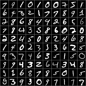
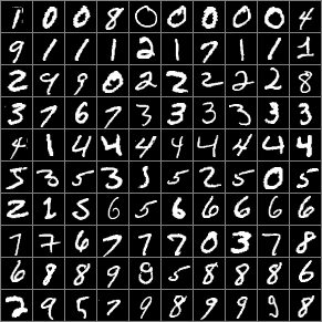
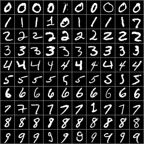
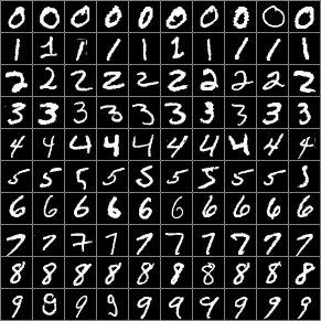
8.1 Particle flow convergence

In this example, we minimize $W_{Y,\beta}(P_{Y,X},P_{Y,Z})$ for the empirical measures We consider the particle flow, i.e., the flow from $(Y,Z)$ to $(Y,X)$ for empirical distributions, where we compute a particle flow [4] from $(Y,Z)$ to $(Y,X)$. We follow a particle flow path, i.e., we define a curve $z(0)_{i}\sim\mathcal{N}(0,I)$ which follows

$$\dot{z}(t)=-\eta\nabla_{z(t)}\mathcal{D}\left(\frac{1}{n}\sum_{i=1}^{n}\delta_{y_{i},x_{i}},\frac{1}{n}\sum_{i=1}^{n}\delta_{y_{i},z(t)_{i}}\right),$$

for an appropriate "distance" $\mathcal{D}$, step size $\eta$ and given joint samples $(y_{i},x_{i})_{i=1}^{n}$. We choose $\mathcal{D}$ as an approximation of $W_{2,\beta}$ by rescaling $Y$ and using the Sinkorn divergence as the sample based distance measure [21, 19], where the "blur" parameter is chosen so small that it is close to the Wasserstein distance. This way we can numerically verify the convergence in Proposition 10. Note that there are no neural networks involved in this example.

We see in Fig. 1 that increasing $\beta$ indeed yields plans which transport no mass in $Y$-direction anymore, which has the consequence that the generated images fit the corresponding label. It can be seen that for $\beta=5$ each row only has one type of digit.

Refer to caption

$\beta=1$

Refer to caption

$\beta=3$

Refer to caption

$\beta=4$

Refer to caption

$\beta=5$

Figure 1: Class conditional MNIST particle flow for different choices of $\beta$. With increasing $\beta$ the labels are better fitted.

8.2 GMM example

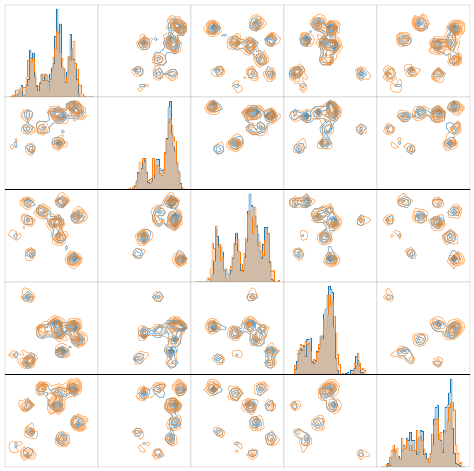
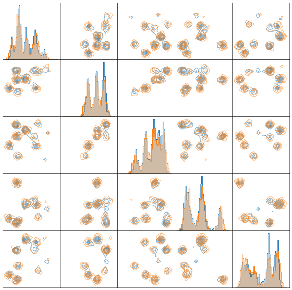
Here we use an experimental setup from [26]: in (1), we choose $P_{X}$ to be a GMM in $\mathbb{R}^{5}$ with 10 mixture components, uniformly chosen means in $[-1,1]$ and standard deviation 0.1. We apply linear diagonal forward model $f=(f_{i,j})_{i,j=1}^{5}$ with $f_{i,i}=\frac{0.1}{i+1}$ and zero components otherwise and Gaussian noise with standard deviation $0.1$. This yields a posterior measure $P_{X|Y=y}$ which is a also a GMM [26, Lemma 11]. Therefore we can sample and evaluate the true posterior as groundtruth. We train a diagonal Bayesian flow matching model according to $L_{Y,FM}$ and our OT Bayesian flow matching according to $L_{Y,OT}$ with POT [20] for the same amount of time on a fixed dataset of size $10000$, where we choose the best model according to a validation set of size $2000$. We parameterize both models with around 140k parameters. We evaluate them using the Sinkhorn distance [21, 19] with the package GeomLoss averaged with 100 posteriors and over 10 training and test runs with randomly sampled mixtures. The sampling is done via an explicit Euler discretization of 10 steps. Our proposed model trained according to $L_{Y,OT}$ with $\beta=20$ obtains an average Sinkhorn distance of 0.0235, whereas the naive model obtains a value of 0.0255. In Figure 2 one can see that both models approximate the posterior very well.

Refer to caption
Refer to caption
Refer to caption
Refer to caption
Figure 2: Posterior histograms for different methods with diagonal Bayesian flow matching on the left and our OT Bayesian flow matching on the right. Ground truth posterior is in orange and model prediction in blue.

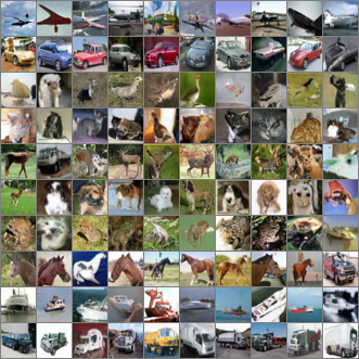
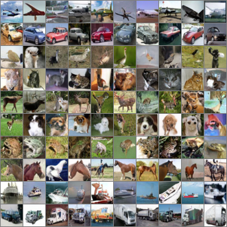
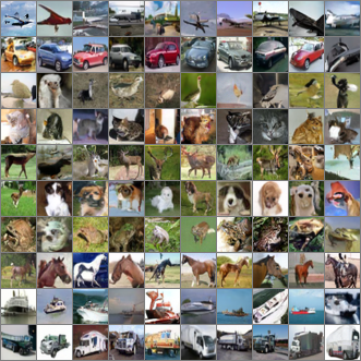
8.3 Class conditional image generation

Refer to caption

$\beta=1$

Refer to caption

$\beta=3$

Refer to caption

$\beta=5$

Refer to caption

$\beta=20$

Refer to caption

$\beta=100$

Refer to caption

diagonal

1 3 5 20 100 diagonal
FID (AD) 5.3 5.1 4.79 4.57 4.38 5.34
FID (Euler) 11.18 11.05 10.82 10.13 9.98 10.76
Figure 3: Class Conditional CIFAR results for different choices of $\beta$ and for the diagonal couplings. Additionally FID results are reported using an adaptive step size solver (AD) and an Euler scheme with 20 steps (Euler).

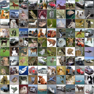
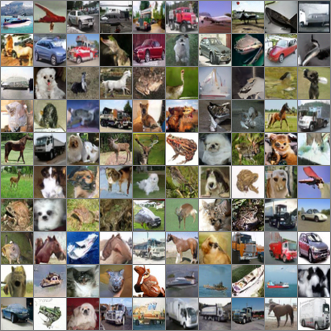
We apply our Bayesian OT flow matching for conditional image generation. We choose the condition $Y$ to be the class labels in order to generate samples of CIFAR10 for a given class. We simulate the flows for different values of $\beta$, by which we mean that we rescale the $Y$-component by $\beta$ as mentioned in Remark 11. We also simulate flows using the "diagonal" plans which coincide with the diagonal Bayesian flow matching objective [53]. For high quality inference we use an adaptive step size solver (Runge-Kutta of order 5). We also compare quantitatively when sampling with a Euler scheme with 20 steps. The samples in Fig. 3 are generated using the adaptive step size solver and sorted by class labels. For low values of $\beta$ we see that the resulting samples do not match their class labels, increasing $\beta$ leads to accurate class representations. The samples are generated given the labels of the training samples, therefore we see improved FID results as $\beta$ increases. The diagonal flow matching objective has the correct class representations, however since the associated couplings are not optimal our experiments suggest that this leads to higher variance during training and therefore slightly lower image quality, see [50] for more details on the advantages of OT based flow matching. We evaluate the methods on a fixed number of epochs, for completeness we note that the diagonal method improves to an FID (AD) of 4.88 under additional training.

9 Conclusions

Inspired from applications in Bayesian inverse problems, we introduced conditional Wasserstein distances. We managed to rewrite these distances as expectations of the Wasserstein distances with respect to the observation. Therefore we are able to directly infer posterior guarantees when trained with the corresponding losses. Furthermore, we calculated the dual of the conditional Wasserstein-1 distance, when the probability measures are compactly supported and recovered well-known conditional Wasserstein GAN losses. We established corresponding velocity fields in the gradient flow theory and used our results to design a new Bayesian flow matching algorithm. Theoretically, improving Proposition 8 for non-discrete $P_{Y}$ distributions would be the next step. In particular one would need to show measurability of the "conditional Monge maps", which does not seem to be easy. Further, from a practical viewpoint, a clear use case would be in conditional domain translation, i.e., when the latent distribution is not a standard Gaussian, but given by some data distribution. There, finding a good OT matching and making use of our proposed framework could improve existing algorithms.
Acknowledgement: P. Hagemann acknowledges funding from from the DFG within the project SPP 2298 "Theoretical Foundations of Deep Learning", C. Wald and G. Steidl gratefully acknowledge funding by the DFG within the SFB “Tomography Across the Scales” (STE 571/19-1, project number: 495365311).

References

  • [1] J. Adler and O. Öktem. Deep Bayesian inversion. arXiv preprint arXiv:1811.05910, 2018.
  • [2] J. Alfonso, R. Baptista, A. Bhakta, N. Gal, A. Hou, I. Lyubimova, D. Pocklington, J. Sajonz, G. Trigila, and R. Tsai. A generative flow for conditional sampling via optimal transport. arXiv preprint arXiv:2307.04102, 2023.
  • [3] F. Altekrüger, P. Hagemann, and G. Steidl. Conditional generative models are provably robust: Pointwise guarantees for Bayesian inverse problems. Transactions on Machine Learning Research, 2023.
  • [4] F. Altekrüger, J. Hertrich, and G. Steidl. Neural Wasserstein gradient flows for discrepancies with riesz kernels. In A. Krause, E. Brunskill, K. Cho, B. Engelhardt, S. Sabato, and J. Scarlett, editors, Proceedings of the 40th International Conference on Machine Learning, volume 202 of Proceedings of Machine Learning Research, pages 664–690. PMLR, 23–29 Jul 2023.
  • [5] L. Ambrosio, E. Brué, and D. Semola. Lectures on Optimal Transport. UNITEXT. Springer International Publishing, 2021.
  • [6] L. Ambrosio, N. Gigli, and G. Savaré. Gradient flows: in metric spaces and in the space of probability measures. Springer Science & Business Media, 2005.
  • [7] L. Ardizzone, C. Lüth, J. Kruse, C. Rother, and U. Köthe. Guided image generation with conditional invertible neural networks. arXiv preprint arXiv:1907.02392, 2019.
  • [8] M. Arjovsky, S. Chintala, and L. Bottou. Wasserstein generative adversarial networks. In International Conference on Machine Learning, pages 214–223. PMLR, 2017.
  • [9] J. Aubin and I. Ekeland. Applied Nonlinear Analysis. Dover Books on Mathematics Series. Dover Publications, 2006.
  • [10] G. Basso. A hitchhikers guide to Wasserstein distances. Online manuscript available at https://api.semanticscholar.org/CorpusID:51801464, 2015.
  • [11] V. Bogachev. Weak convergence of measures. Springer Berlin Heidelberg, Berlin, Heidelberg, 2007.
  • [12] C. Bunne, A. Krause, and M. Cuturi. Supervised training of conditional Monge maps. In A. H. Oh, A. Agarwal, D. Belgrave, and K. Cho, editors, Advances in Neural Information Processing Systems, 2022.
  • [13] J. Chemseddine, P. Hagemann, and C. Wald. Y-diagonal couplings: Approximating posteriors with conditional Wasserstein distances. arXiv preprint arXiv:2310.13433v, 2023.
  • [14] R. T. Chen, Y. Rubanova, J. Bettencourt, and D. K. Duvenaud. Neural ordinary differential equations. Advances in neural information processing systems, 31, 2018.
  • [15] R. T. Q. Chen. torchdiffeq, 2018.
  • [16] T. Cover. Elements of Information Theory. John Wiley & Sons, Ltd, 2005.
  • [17] L. Deng. The MNIST database of handwritten digit images for machine learning research. IEEE Signal Processing Magazine, 29(6):141–142, 2012.
  • [18] C. Du, T. Li, T. Pang, S. Yan, and M. Lin. Nonparametric generative modeling with conditional sliced Wasserstein flows. arxiv preprint arXiv:2305.02164, 2023.
  • [19] J. Feydy, T. Séjourné, F.-X. Vialard, S.-i. Amari, A. Trouvé, and G. Peyré. Interpolating between Optimal Transport and MMD using Sinkhorn divergences. In The 22nd International Conference on Artificial Intelligence and Statistics, pages 2681–2690. PMLR, 2019.
  • [20] R. Flamary, N. Courty, A. Gramfort, M. Z. Alaya, A. Boisbunon, S. Chambon, L. Chapel, A. Corenflos, K. Fatras, N. Fournier, et al. Pot: Python Optimal Transport. The Journal of Machine Learning Research, 22(1):3571–3578, 2021.
  • [21] A. Genevay, G. Peyre, and M. Cuturi. Learning generative models with Sinkhorn divergences. In Proceedings of the Twenty-First International Conference on Artificial Intelligence and Statistics, volume 84 of Proceedings of Machine Learning Research, pages 1608–1617. PMLR, 09–11 Apr 2018.
  • [22] Y. geun Kim, K. Lee, Y. Choi, J.-H. Won, and M. C. Paik. Wasserstein geodesic generator for conditional distributions. arXiv preprint arXiv:2308.10145, 2023.
  • [23] N. Gigli. On the geometry of the space of probability measures endowed with the quadratic Optimal Transport distance. PhD Thesis, 2008. cvgmt preprint.
  • [24] P. Hagemann, J. Hertrich, F. Altekrüger, R. Beinert, J. Chemseddine, and G. Steidl. Posterior sampling based on gradient flows of the MMD with negative distance kernel. Proceedings ICLR, 2024.
  • [25] P. Hagemann, J. Hertrich, and G. Steidl. Generalized normalizing flows via Markov chains. In Non-local Data Interactions: Foundations and Applications. Cambridge University Press, 2022.
  • [26] P. Hagemann, J. Hertrich, and G. Steidl. Stochastic normalizing flows for inverse problems: A Markov chains viewpoint. SIAM/ASA Journal on Uncertainty Quantification, 10(3):1162–1190, 2022.
  • [27] J. Hertrich, M. Gräf, R. Beinert, and G. Steidl. Wasserstein steepest descent flows of discrepancies with Riesz kernels. Journal of Mathematical Analysis and Applications, 2023.
  • [28] M. Heusel, H. Ramsauer, T. Unterthiner, B. Nessler, and S. Hochreiter. GANs trained by a two time-scale update rule converge to a local nash equilibrium. In I. Guyon, U. V. Luxburg, S. Bengio, H. Wallach, R. Fergus, S. Vishwanathan, and R. Garnett, editors, Advances in Neural Information Processing Systems, volume 30. Curran Associates, Inc., 2017.
  • [29] B. Hosseini, A. W. Hsu, and A. Taghvaei. Conditional optimal transport on function spaces. arXiv preprint arXiv:2311.05672, 2024.
  • [30] A. Hyvärinen and P. Dayan. Estimation of non-normalized statistical models by score matching. Journal of Machine Learning Research, 6(4), 2005.
  • [31] Y.-g. Kim, K. Lee, and M. C. Paik. Conditional Wasserstein generator. IEEE Transactions on Pattern Analysis and Machine Intelligence, 45(6):7208–7219, 2023.
  • [32] D. P. Kingma and J. Ba. Adam: a method for stochastic optimization. In Proceedings of the ICLR ’15, 2015.
  • [33] H. Knothe. Contributions to the theory of convex bodies. Michigan Mathematical Journal, 4(1):39 – 52, 1957.
  • [34] A. Krizhevsky, G. Hinton, et al. Learning multiple layers of features from tiny images. 2009.
  • [35] Y. Lipman, R. T. Q. Chen, H. Ben-Hamu, M. Nickel, and M. Le. Flow matching for generative modeling. In The Eleventh International Conference on Learning Representations, 2023.
  • [36] X. Liu, C. Gong, and qiang liu. Flow straight and fast: Learning to generate and transfer data with rectified flow. In The Eleventh International Conference on Learning Representations, 2023.
  • [37] P. Manupriya, R. K. Das, S. Biswas, S. Chandhok, and S. N. Jagarlapudi. Empirical Optimal Transport between conditional distributions. arXiv preprint arXiv:2305.15901, 2023.
  • [38] J. Martin. About exchanging expectation and supremum for conditional Wasserstein GANs. arXiv preprint arXiv:2103.13906, 2021.
  • [39] R. J. McCann. A convexity principle for interacting gases. Advances in Mathematics, 128(1):153–179, 1997.
  • [40] M. Mirza and S. Osindero. Conditional Generative Adversarial Nets. arXiv preprint arXiv:1411.1784, 2014.
  • [41] T. Nguyen, V. Nguyen, T. Le, H. Zhao, Q. H. Tran, and D. Phung. Cycle class consistency with distributional Optimal Transport and knowledge distillation for unsupervised domain adaptation. In The 38th Conference on Uncertainty in Artificial Intelligence, 2022.
  • [42] A. Q. Nichol and P. Dhariwal. Improved denoising diffusion probabilistic models. In International conference on machine learning, pages 8162–8171. PMLR, 2021.
  • [43] G. Peyré and M. Cuturi. Computational Optimal Transport: With applications to data science. Foundations and Trends in Machine Learning, 11(5-6):355–607, 2019.
  • [44] A.-A. Pooladian, H. Ben-Hamu, C. Domingo-Enrich, B. Amos, Y. Lipman, and R. Chen. Multisample flow matching: Straightening flows with minibatch couplings. arXiv preprint arXiv:2304.14772, 2023.
  • [45] A. Rakotomamonjy, R. Flamary, G. Gasso, M. E. Alaya, M. Berar, and N. Courty. Optimal Transport for conditional domain matching and label shift. Mach. Learn., 111(5):1651–1670, May 2022.
  • [46] M. Rosenblatt. Remarks on a Multivariate Transformation. The Annals of Mathematical Statistics, 23(3):470 – 472, 1952.
  • [47] F. Santambrogio. Optimal Transport for applied mathematicians. Birkäuser, NY, 55(58-63):94, 2015.
  • [48] E. G. Tabak, G. Trigila, and W. Zhao. Data driven conditional Optimal Transport. Machine Learning, 110:3135–3155, 2021.
  • [49] J. Thickstun. Kantorovich-Rubinstein duality. Online manuscript available at https://courses.cs.washington.edu/courses/cse599i/20au/resources/L12_duality.pdf.
  • [50] A. Tong, N. Malkin, G. Huguet, Y. Zhang, J. Rector-Brooks, K. Fatras, G. Wolf, and Y. Bengio. Improving and generalizing flow-based generative models with minibatch optimal transport. In ICML Workshop on New Frontiers in Learning, Control, and Dynamical Systems, 2023.
  • [51] C. Villani. Optimal Transport: Old And New, volume 338. Springer, 2009.
  • [52] P. Vincent. A connection between score matching and denoising autoencoders. Neural Computation, 23(7):1661–1674, 2011.
  • [53] J. B. Wildberger, M. Dax, S. Buchholz, S. R. Green, J. H. Macke, and B. Schölkopf. Flow matching for scalable simulation-based inference. In Thirty-seventh Conference on Neural Information Processing Systems, 2023.
  • [54] C. Winkler, D. Worrall, E. Hoogeboom, and M. Welling. Learning likelihoods with conditional normalizing flows. arXiv preprint arXiv:1912.00042, 2019.
  • [55] Q. Zheng, M. Le, N. Shaul, Y. Lipman, A. Grover, and R. T. Q. Chen. Guided flows for generative modeling and decision making. arXiv preprint arXiv:2311.13443, 2023.

Appendix A Counterexample for equality in equation 2

$\delta_{y_{1},x_{1}}$ $\delta_{y_{1},z_{1}}$ $\delta_{y_{2},z_{2}}$ $\delta_{y_{2},x_{2}}$
Figure 4: Visualization of the example. The blue dots belong to $P_{Y,X}$ and the red dots to $P_{Y,Z}$. The optimal coupling is the solid line, while the ”diagonal” coupling is the dotted one.

We provide a simple example showing that we cannot expect equality in (2). Recall that for two empirical measures $\mu=\frac{1}{n}\sum_{i=1}^{n}\delta_{a_{i}}$ and $\nu=\frac{1}{n}\sum_{i=1}^{n}\delta_{b_{i}}$, $a_{i},b_{i}\in\mathbb{R}^{d}$, the Wasserstein-$p$ distance, $p\in[1,\infty)$ can be written as

$\displaystyle W_{p}^{p}(\mu,\nu)=\inf_{\sigma\in\mathcal{S}_{n}}\frac{1}{n}\sum_{i=1}^{n}\|a_{i}-b_{\sigma(i)}\|^{p},$ (32)

where $\mathcal{S}_{n}$ is the set of permutations on $\{1,\ldots,n\}$, see [43, Proposition 2.1].

On the probability space $(\Omega,\mathcal{A},\mathbb{P})$ with $\Omega=\{\omega_{1},\omega_{2}\}$, $\mathcal{A}=2^{\Omega}$ and $\mathbb{P}(\omega_{1})=\mathbb{P}(\omega_{2})=\frac{1}{2}$, we define the random variables $X,Y:\Omega\to\mathbb{R}$ by

$X$ $Y$ $Z$
$\omega_{1}$ 0 0 $n$
$\omega_{2}$ $n$ 1 0

,       $n>1$.

Then we have

$\displaystyle P_{Y,X}=\frac{1}{2}\delta_{0,0}+\frac{1}{2}\delta_{1,n},\quad P_{Y,Z}=\frac{1}{2}\delta_{1,0}+\frac{1}{2}\delta_{0,n}$

which implies by (32) that

$\displaystyle W_{1}(P_{Y,X},P_{Y,Z})$ $\displaystyle=\frac{1}{2}\min\big{\{}\|(0,0)-(1,0)\|+\|(1,n)-(0,n)\|,$
$\displaystyle\qquad\qquad\|(0,0)-(0,n)\|+\|(1,n)-(1,0)\|\big{\}}=1.$

On the other hand, we get

$$P_{X|Y=0}=\delta_{0},\quad P_{X|Y=1}=\delta_{n},\quad P_{Z|Y=0}=\delta_{n},\quad P_{Z|Y=1}=\delta_{0},\quad P_{Y}=\frac{1}{2}\delta_{0}+\frac{1}{2}\delta_{1},$$

so that

$\displaystyle\mathbb{E}_{y}[W_{1}(P_{X|Y=y},P_{Z|Y=y})]=n=nW_{1}(P_{Y,X},P_{Y,Z}).$

Note that if we forbid the coupling to move mass across the $y$-direction, we actually would obtain equality, which motivates our definition of conditional Wasserstein distance, for an illustration see Fig. 4.

Note that in [31], the summation metric is considered, i.e. $\|(x_{1},y_{1})-(x_{2},y_{2})\|_{sum}=\|x_{1}-x_{2}\|+\|y_{1}-y_{2}\|$ for which our counterexample is still valid.

Appendix B Proofs of Section 3

Proof of Proposition 1. i) First we show $\geq$. Let $\alpha_{y_{1},y_{2}}$ be the disintegration of some $\alpha\in\Gamma_{Y}^{4}(P_{Y,X},P_{Y,Z})$ with respect to $\pi^{1,3}_{\sharp}\alpha$. Then we obtain

$\displaystyle I(\alpha)$ $\displaystyle=\int_{(A\times B)^{2}}\|(y_{1},x_{1})-(y_{2},x_{2})\|^{p}\,\mathrm{d}\alpha(y_{1},x_{1},y_{2},x_{2})$ (33)
$\displaystyle=\int_{A^{2}}\int_{B^{2}}\|(y_{1},x_{1})-(y_{2},x_{2})\|^{p}\,\mathrm{d}\alpha_{y_{1},y_{2}}(x_{1},x_{2})\mathrm{d}\pi^{1,3}_{\sharp}\alpha(y_{1},y_{2})$ (34)
$\displaystyle=\int_{A^{2}}\int_{B^{2}}\|(y_{1},x_{1})-(y_{2},x_{2})\|^{p}\,\mathrm{d}\alpha_{y_{1},y_{2}}(x_{1},x_{2})\,\mathrm{d}\Delta_{\sharp}P_{Y}(y_{1},y_{2})$ (35)
$\displaystyle=\int_{A}\int_{B^{2}}\|(y,x_{1})-(y,x_{2})\|^{p}\,\mathrm{d}\alpha_{y,y}(x_{1},x_{2})\mathrm{d}P_{Y}(y)$ (36)
$\displaystyle=\int_{A}\int_{B^{2}}\|x_{1}-x_{2}\|^{p}\,\mathrm{d}\alpha_{y,y}(x_{1},x_{2})\mathrm{d}P_{Y}(y).$ (37)

Next, we show that $\alpha_{y,y}\in\Gamma(P_{X|Y=y},P_{Z|Y=y})$ a.e., which means $\pi^{1}_{\sharp}\alpha_{y,y}=P_{X|Y=y}$ and $\pi^{2}_{\sharp}\alpha_{y,y}=P_{Z|Y=y}$ a.e.. Using (7), we obtain indeed for all Borel measurable functions $f:A\times B\to[0,\infty]$ that

$\displaystyle\int_{A}\int_{B}f(y,x_{1})\,\mathrm{d}\pi^{1}_{\sharp}(\alpha_{y,y})(x_{1})\mathrm{d}P_{Y}(y)$ $\displaystyle=\int_{A^{2}}\int_{B}f(y_{1},x_{1})\,\mathrm{d}\pi^{1}_{\sharp}\alpha_{y_{1},y_{2}}(x_{1})\,\mathrm{d}(\Delta)_{\sharp}P_{Y}(y_{1},y_{2})$
$\displaystyle=\int_{A^{2}}\int_{B}f(y_{1},x_{1})\,\mathrm{d}\pi^{1}_{\sharp}(\alpha_{y_{1},y_{2}})(x_{1})\,\mathrm{d}\pi^{1,3}_{\sharp}\alpha(y_{1},y_{2})$
$\displaystyle=\int_{A^{2}\times B^{2}}f(y_{1},x_{1})\,\mathrm{d}\alpha_{y_{1},y_{2}}(x_{1},x_{2})\,\mathrm{d}\pi^{1,3}_{\sharp}\alpha(y_{1},y_{2})$
$\displaystyle=\int_{A^{2}\times B^{2}}f(y_{1},x_{1})\,\mathrm{d}\alpha=\int_{A\times B}f(y_{1},x_{1})\,\mathrm{d}\pi^{1,2}_{\sharp}\alpha(y_{1},x_{1})$
$\displaystyle=\int_{A\times B}f(y_{1},x_{1})\,\mathrm{d}P_{Y,X}(y_{1},x_{1}).$

Consequently, we have $I(\alpha)\geq\mathbb{E}_{y\sim P_{Y}}{\mathbb{E}}\big{[}W_{p}^{p}(P_{X|Y=y},P_{Z|Y=y})\big{]}$ and since $W_{p,Y}^{p}(P_{Y,X},P_{Y,Z})=\inf_{\alpha}I(\alpha)$, this gives assertion.

Now we prove the opposite direction $\leq$. For any $y\in A$, let $\alpha_{y}\in\Gamma(P_{X|Y=y},P_{Z|Y=y})$ be an optimal plan, i.e.

$$\mathcal{W}_{p}^{p}(P_{X|Y=y},P_{Z|Y=y})=\int_{B^{2}}\|x_{1}-x_{2}\|^{p}\,\mathrm{d}\alpha_{y}(x_{1},x_{2}).$$

This implies

$$\int_{A}\mathcal{W}_{p}^{p}(P_{X|Y=y},P_{Z|Y=y})\,\mathrm{d}P_{Y}(y)=\int_{A}\int_{B^{2}}\|x_{1}-x_{2}\|^{p}\,\mathrm{d}\alpha_{y,y}(x_{1},x_{2})\mathrm{d}P_{Y}(y).$$ (38)

ii) For an optimal $\alpha\in\Gamma_{Y}^{4}(P_{Y,X},P_{Y,Z})$, we have by Part i) and (37) that

$\displaystyle W_{p,Y}^{p}(P_{Y,X},P_{Y,Z})$ $\displaystyle=\int_{A}W_{p}^{p}(P_{X|Y=y},P_{Z|Y=y})\,\mathrm{d}P_{y}(y)$ (39)
$\displaystyle=\int_{A}\int_{B^{2}}\|x_{1}-x_{2}\|^{p}\,\mathrm{d}\alpha_{y,y}(x_{1},x_{2})\mathrm{d}P_{Y}(y).$ (40)

Hence we get

$$0=\int_{A}\Big{(}\int_{B^{2}}\|x_{1}-x_{2}\|^{p}\,\mathrm{d}\alpha_{y,y}(x_{1},x_{2})-W_{p}^{p}(P_{X|Y=y},(P_{Z|Y=y})\Big{)}\,\mathrm{d}P_{Y}(y).$$

The inner integrand is nonnegative which finally implies that it is zero $P_{Y}$-a.e. and therefore $\alpha_{y,y}$ is an optimal plan in $W_{p}(P_{X|Y=y},P_{Z|Y=y})$.
iii) Let $\alpha$ be defined by (11), i.e.,

$\displaystyle\int\limits_{(A\times B)^{2}}f(y_{1},x_{1},y_{2},x_{2})\,\mathrm{d}\alpha(y_{1},x_{1},y_{2},x_{2})$
$\displaystyle=\int\limits_{A}\int\limits_{A\times B^{2}}f(y_{1},x_{1},y_{2},x_{2})\,\mathrm{d}(\delta_{y_{1}}\times\alpha_{y_{1}})(y_{2},x_{1},x_{2})\mathrm{d}P_{Y}(y_{1})$

for all Borel measurable functions $f:(A\times B)^{2}\to[0,+\infty]$. Indeed $\alpha$ is a well defined probability measure on $(A\times B)^{2}$ by the following reasons: by [6, Lemma 12.4.7], we can choose a Borel family $(\alpha_{y})_{y}$. For any Borel set $\mathcal{S}\subseteq A\times B\times B$, we have

$\displaystyle(\delta_{y}\times\alpha_{y})(\mathcal{S})=\int_{A\times B^{2}}1_{\mathcal{S}}(\tilde{y},x_{1},x_{2})\,\mathrm{d}(\delta_{y}\times\alpha_{y})(\tilde{y},x_{1},x_{2})=\int_{B^{2}}1_{\mathcal{S}}(y,x_{1},x_{2})\,\mathrm{d}\alpha_{y}.$ (41)

By [6, Equation 5.3.1] the function $y\mapsto\int_{B^{2}}1_{\mathcal{S}}(y,x_{1},x_{2})\mathrm{d}\alpha_{y}$ is Borel measurable. Consequently also $y\mapsto\delta_{y}\times\alpha_{y}(\mathcal{S})$ is Borel measurable and thus $\alpha$ is well defined. Then (38) can be rewritten as

$$\int_{A}\mathcal{W}_{p}^{p}(P_{X|Y=y},P_{Z|Y=y})\,\mathrm{d}P_{Y}(y)=\int_{(A\times B)^{2}}\|(y_{1},x_{1})-(y_{2},x_{2})\|^{p}\,\mathrm{d}\alpha(y_{1},x_{1},y_{2},x_{2}).$$ (42)

It remains to show that $\alpha\in\Gamma_{Y}(P_{Y,X},P_{Y,Z})$ which means $\pi^{1,3}_{\sharp}\alpha=\Delta_{\sharp}P_{Y}$, $\pi^{1,2}_{\sharp}\alpha=P_{Y,X}$ and $\pi^{3,4}_{\sharp}\alpha=P_{Y,Z}$. The first equality follows from

$\displaystyle\int_{A^{2}}f(y_{1},y_{2})\mathrm{d}\pi^{1,3}_{\sharp}\alpha$ $\displaystyle=\int_{(A\times B)^{2}}(f\circ\pi^{1,3})(y_{1},x_{1},y_{2},x_{2})\,\mathrm{d}\alpha(y_{1},x_{1},y_{2},x_{2})$
$\displaystyle=\int_{(A\times B)^{2}}f(y_{1},y_{2})\,\mathrm{d}\delta_{y_{1}}(y_{2})\,\mathrm{d}\alpha_{y_{1}}(x_{1},x_{2})\mathrm{d}P_{Y}(y_{1})$
$\displaystyle=\int_{A}f(y,y)\,\mathrm{d}P_{Y}(y)=\int_{A^{2}}f(y_{1},y_{2})\,\mathrm{d}(\Delta_{\sharp}P_{Y})(y_{1},y_{2})$

for all Borel functions $f:A^{2}\to[0,+\infty]$, and the second one from

$\displaystyle\int_{A\times B}f(y,x)\mathrm{d}\pi^{1,2}_{\sharp}\alpha(y,x)$ $\displaystyle=\int_{(A\times B)^{2}}f(y_{1},x_{1})\,\mathrm{d}\delta_{y_{1}}(y_{2})\mathrm{d}\alpha_{y_{1}}(x_{1},x_{2})\mathrm{d}P_{Y}(y_{1})$ (43)
$\displaystyle=\int_{A\times B}f(y,x)\mathrm{d}\pi^{1}_{\sharp}\alpha_{y}(x)\,\mathrm{d}P_{Y}(y)$ (44)
$\displaystyle=\int_{A\times B}f(y,x)\mathrm{d}P_{X|Y=y}(x)\,\mathrm{d}P_{Y}(y)$ (45)
$\displaystyle=\int_{A\times B}f(y,x)\,\mathrm{d}P_{Y,X}(y,x)$ (46)

for all Borel functions $f:A\times B\to[0,+\infty]$. The third equality follows analogously.

The final assertion follows from (42) and the equality relation (10). $\Box$
Proof of Proposition 12. Let $\kappa:A\times B^{2}\to(A\times B)^{2}$ be defined by $(y,x_{1},x_{2})\mapsto(y,x_{1},y,x_{2})$. We show that $\kappa_{\sharp}:\Gamma_{Y}^{3}(P_{Y,X},P_{Y,Z})\to\Gamma^{4}_{Y}(P_{Y,X},P_{Y,Z})$ is the inverse of $\pi^{1,2,4}_{\sharp}$. Since $\text{Id}_{(A\times B^{2})}=\pi^{1,2,4}\circ(\Delta\circ\pi^{1},\pi^{2},\pi^{3})$, it remains to show that $\kappa_{\sharp}\circ\pi^{1,2,4}_{\sharp}=\text{Id}_{\Gamma_{Y}^{4}(P_{Y,X},P_{Y,Z})}$. For $\alpha\in\Gamma^{4}(P_{Y,X},P_{Y,Z})$ and Borel measurable function $f:(A\times B)^{2}\to[0,+\infty]$, we have

$\displaystyle\int_{(A\times B)^{2}}f(y_{1},x_{1},y_{2},x_{2})\,\mathrm{d}\kappa_{\sharp}\pi^{1,2,4}_{\sharp}\alpha=\int_{(A\times B)^{2}}f(y_{2},x_{1},y_{2},x_{2})\,\mathrm{d}\alpha(y_{1},x_{1},y_{2},x_{2})$
$\displaystyle=\int_{A^{2}}\int_{B^{2}}f(y_{2},x_{1},y_{2},x_{2})\,\mathrm{d}\alpha_{y_{1},y_{2}}(x_{1},x_{2})\mathrm{d}\pi^{1,3}_{\sharp}\alpha(y_{1},y_{2})$
$\displaystyle=\int_{(A\times B)^{2}}f(y_{1},x_{1},y_{2},x_{2})\,\mathrm{d}\alpha_{y_{1},y_{2}}(x_{1},x_{2})\mathrm{d}\Delta_{\sharp}P_{Y}(y_{1},y_{2})$
$\displaystyle=\int_{(A\times B)^{2}}f(y_{1},x_{1},y_{2},x_{2})\,\mathrm{d}\alpha.$

The second claim follows by

$\displaystyle\int_{(A\times B)^{2}}\|(y_{1},x_{1})-(y_{2},x_{2})\|^{p}\,\mathrm{d}\alpha=\int_{A^{2}}\int_{B^{2}}\|(y_{1},x_{1})-(y_{2},x_{2})\|^{p}\,\mathrm{d}\alpha_{y_{1},y_{2}}\mathrm{d}\pi^{1,3}_{\sharp}\alpha(y_{1},y_{2})$
$\displaystyle=\int_{A^{2}}\int_{B^{2}}\|(y_{1},x_{1})-(y_{2},x_{2})\|^{p}\,\mathrm{d}\alpha_{y_{1},y_{2}}\mathrm{d}\Delta_{\sharp}P_{Y}(y_{1},y_{2})$
$\displaystyle=\int_{A}\int_{B^{2}}\|(y,x_{1})-(y,x_{2})\|^{p}\mathrm{d}\alpha_{y,y}\mathrm{d}P_{Y}(y)$
$\displaystyle=\int_{A}\int_{B^{2}}\|x_{1}-x_{2}\|^{p}\,\mathrm{d}\pi^{2,3,4}_{\sharp}\alpha.\qquad\Box$

Appendix C Proofs of Section 4

The proof uses similar arguments as the short notes [49] and [10], which are derivations for the dual for the "usual" Wasserstein distance. We adapt these ideas for our conditional Wasserstein distance.
Proof of Proposition 4. Let $C_{b}=C_{b}(A\times B)$ be the space of continuous bounded functions on $A\times B$ and $\mathcal{S}$ the set of nonnegative finite Borel measures $\alpha$ on $(A\times B)^{2}$ which are supported at most on the y-diagonal. By [47, Section 1.2], we know that

$\displaystyle\sup_{f,g\in C_{b}(A\times B)}\mathbb{E}_{Y,X}[f]+\mathbb{E}_{Y,Z}[g]-\int_{(A\times B)^{2}}(f+g)\,\mathrm{d}\alpha=\begin{cases}0\quad\text{ if }\alpha\in\Gamma(P_{Y,X},P_{Y,Z}),\\ \infty\quad\text{otherwise}.\end{cases}$

Using this relation, we obtain

$\displaystyle W_{1,Y}(P_{Y,X},P_{Y,Z})$ $\displaystyle=\inf_{\alpha\in\Gamma_{Y}^{4}}\int\|(y_{1},x_{1})-(y_{2},x_{2})\|\,\mathrm{d}\alpha$
$\displaystyle=\inf_{\alpha\in\mathcal{S}}\sup_{f,g\in C_{b}}L(\alpha,f,g)$

with the Lagrangian

$\displaystyle L(\alpha,f,g)$ $\displaystyle\coloneqq\mathbb{E}_{Y,X}[f]+\mathbb{E}_{Y,Z}[g]$ (47)
$\displaystyle\quad+\underset{(A\times B)^{2}}{\int}\|(y_{1},x_{1})-(y_{2},x_{2})\|-f(y_{1},x_{1})-g(y_{2},x_{2})\,\mathrm{d}\alpha.$ (48)

By Corollary 15 below, strong duality holds true, so that we can exchange infimum and supremum to get

$$W_{1,Y}(P_{Y,X},P_{Y,Z})=\sup_{f,g\in C_{b}}\inf_{\alpha\in\mathcal{S}}L(\alpha,f,g).$$

From this, we see that the optimal $f,g$ have to fulfill

$\displaystyle f(y,x_{1})+g(y,x_{2})\leq\|x_{1}-x_{2}\|$ (49)

for all $y\in A$, since otherwise the attained infimum is $-\infty$. Therefore we have for the optimal $f,g$ that $L(\alpha,f,g)\geq\mathbb{E}_{Y,X}[f]+\mathbb{E}_{Y,Z}[g]$ and choosing the plan $\alpha=0\in\mathcal{S}$, we obtain

$$\inf_{\alpha\in\mathcal{S}}L(\alpha,f,g)=\mathbb{E}_{P_{Y,X}}[f]+\mathbb{E}_{P_{Y,Z}}[g]$$

for all $(f,g)\in\tilde{\mathcal{F}}$, where

$$\tilde{\mathcal{F}}:=\{(f,g)\in(C_{b}(A\times B))^{2}:f(y,x_{1})+g(y,x_{2})\leq\|x_{2}-x_{2}\|\}.$$

Consequently, we get

$\displaystyle W_{1,Y}(P_{Y,X},P_{Y,Z})=\sup_{(f,g)\in\tilde{\mathcal{F}}}\mathbb{E}_{Y,X}[f]+\mathbb{E}_{Y,Z}[g].$ (50)

For $(f,g)\in\tilde{\mathcal{F}}$, we define $\tilde{f}(y,x)\coloneqq\inf_{u\in B}\|x-u\|-g(y,u)$. Then

$\displaystyle\tilde{f}(y,x)$ $\displaystyle=\inf_{u\in B}\{\|x-u\|-g(y,u)\}$ (51)
$\displaystyle\leq\inf_{u\in B}\{\|x-z\|+\|z-u\|-g(y,u)\}$ (52)
$\displaystyle=\tilde{f}(y,z)+\|x-z\|$ (53)

shows the 1-Lipschitz continuity of $\tilde{f}$ with respect to the second component. Using (49) we obtain that $\tilde{f}(y,x)\geq f(y,x)$. Since $\tilde{f}(y,x)\leq\|x-x\|-g(y,x)$, we conclude

$\displaystyle f(y,x)\leq\tilde{f}(y,x)\leq-g(y,x).$ (54)

Thus, $\tilde{f}$ is bounded. As pointwise infimum over continuous functions, $\tilde{f}$ is upper semicontinuous in $(y,x)$. In summary, we have that $\tilde{f}\in\mathcal{F}$. By (50) and (54), we conclude

$$W_{1,Y}(P_{Y,X},P_{Y,Z})=\sup_{(f,g)\in\tilde{\mathcal{F}}}\left\{\mathbb{E}_{Y,X}[f]+\mathbb{E}_{Y,Z}[g]\right\}\\ \leq\sup_{h\in\mathcal{F}}\left\{\mathbb{E}_{Y,X}[h]-\mathbb{E}_{Y,Z}[h]\right\}$$

and further for $\alpha\in\Gamma^{4}_{Y}(P_{Y,X},P_{Y,Z})\subset\Gamma(P_{Y,X},P_{Y,Z})$ that

$\displaystyle\sup_{h\in\mathcal{F}}\left\{\mathbb{E}_{Y,X}[h]-\mathbb{E}_{Y,Z}[h]\right\}$ $\displaystyle\leq\sup_{h\in\mathcal{F}}\inf_{\alpha\in\Gamma_{Y}^{4}}\int_{(A\times B)^{2}}h(y_{1},x_{1})-h(y_{2},x_{2})\mathrm{d}\alpha$
$\displaystyle=\sup_{h\in\mathcal{F}}\inf_{\alpha\in\Gamma_{Y}^{4}}\int_{(A\times B)^{2}}h(y_{1},x_{1})-h(y_{1},x_{2})\mathrm{d}\alpha$
$\displaystyle\leq\inf_{\alpha\in\Gamma_{Y}^{4}}\int_{(A\times B)^{2}}\|x_{1}-x_{2}\|\mathrm{d}\alpha$
$\displaystyle=\inf_{\alpha\in\Gamma_{Y}^{4}}\int_{(A\times B)^{2}}\|(y_{1},x_{1})-(y_{2},x_{2})\|\mathrm{d}\alpha$
$\displaystyle=W_{1,Y}(P_{Y,X},P_{Y,Z}).$

Thus, $W_{1,Y}(P_{Y,X},P_{Y,Z})=\sup_{h\in\mathcal{F}}\{\mathbb{E}_{Y,X}[h]-\mathbb{E}_{Y,Z}[h]\}$, which finishes the proof. $\Box$

The proof of strong duality relies on the following minimax principle from [9, Theorem 7 Chapter 6].

Theorem 14.

Let $X$ be a convex subset of a topological vector space, and $Y$ be a convex subset of a vector space. Assume $f:X\times Y\to\mathbb{R}$ satisfies the following conditions:

  • i)

    For every $y\in Y$, the map $x\mapsto f(x,y)$ is lower semi continuous and convex.

  • ii)

    There exists $y_{0}$ such that $x\mapsto f(x,y_{0})$ is inf-compact, i.e the set $\{x\in X:f(x,y_{0})\leq a\}$ is relatively compact for each $a\in\mathbb{R}$.

  • iii)

    For every $x\in X$, the map $y\to f(x,y)$ is convex.

Then it holds

$\displaystyle\inf_{x\in X}\sup_{y\in Y}f(x,y)=\sup_{y\in Y}\inf_{x\in X}f(x,y).$

Based on the theorem we can prove the desired strong duality relation.

Corollary 15.

For the Lagrangian in (47) it holds

$\displaystyle\underset{\alpha\in\mathcal{S}}{\mathsf{inf}}\sup_{f,g\in C_{b}}L(\alpha,f,g)=\sup_{f,g\in C_{b}}\underset{\alpha\in\mathcal{S}}{\mathsf{inf}}L(\alpha,f,g).$
Proof.

We will verify the conditions in Theorem 14. Recall that $\mathcal{S}$ is the set of finite nonnegative Borel measures $\alpha$ on $(A\times B)^{2}$ such that there exists a finite nonegative finite measure $\beta$ on $B$ with $\pi^{1,3}_{\sharp}\alpha=\Delta_{\sharp}\beta$. Let $\mathcal{M}$ be the topological vector space of finite signed Borel measures on $(A\times B)^{2}$ with weak convergence topology. Thus, since the pushforward is linear on $\mathcal{S}$, we conclude that $\mathcal{S}$ is a convex subset. Now we use Theorem 14 with $X\coloneqq\mathcal{S}$, $Y\coloneqq C_{b}\times C_{b}$ and $f\coloneqq L$.

Verifying i) The map $\alpha\mapsto L(\alpha,f,g)$ is linear and continuous on $\mathcal{S}$ under the weak convergence of measures. This follows from the fact that the integrand of $\alpha$ in $L(\alpha,f,g)$ is in $C_{b}((A\times B)^{2})$.

Verifying iii) Note that for any $\alpha\in\mathcal{S}$ the map $(f,g)\mapsto L(\alpha,f,g)$ is linear in $(f,g)$ and therefore convex.

Verifying ii) Setting $f(y,x)\coloneqq-1,g(y,x)\coloneqq-1$ for all $(y,x)$, we will show that for any fixed $a\in R$, the set

$$\mathcal{S}_{a}:=\{\alpha\in\mathcal{S}:L(\alpha,-1,-1)\leq a\}$$

is relatively compact. Since the integrand is bounded from below by $2$ and $\mathcal{S}$ only contains nonnegative measures, the measures in $\mathcal{S}_{a}$ are uniformly bounded in the total variation norm, since otherwise

$\displaystyle L(\alpha,-1,-1)=2+\int_{(A\times B)^{2}}\|(y_{1},x_{1})-(y_{2},x_{2})\|+2\,\mathrm{d}\alpha$

can become arbitrary large which contradicts $L(\alpha,-1,-1)\leq a$. Therefore the compactness of $A,B$ implies that $\mathcal{S}_{a}$ is a family of tight measures. By [11, Theorem 8.6.7], the set $\mathcal{S}_{a}$ is relatively compact in the weak topology. ∎

Appendix D Proofs of Section 5

Proof of Proposition 5. i) We have $\mu_{t}\in\mathcal{P}_{p,Y}(\mathbb{R}^{d}\times\mathbb{R}^{m})$ for every $t\in[0,1]$ by

$\displaystyle(\pi^{1})_{\sharp}\mu_{t}=\pi^{1}_{\sharp}(e_{t})_{\sharp}\alpha=((1-t)\pi^{1}+t\pi^{3})_{\sharp}(\pi^{1,3})_{\sharp}\alpha=((1-t)\pi^{1}+t\pi^{2})_{\sharp}\Delta_{\sharp}P_{Y}=P_{Y}.$ (55)

For $s,t\in[0.1]$, let $\alpha_{s,t}\coloneqq(e_{s},e_{t})_{\sharp}\alpha$. By definition we see that $\alpha_{s,t}\in\Gamma(\mu_{s},\mu_{t})$. Further $\pi^{1,3}_{\sharp}\alpha_{s,t}=\Delta_{\sharp}P_{Y}$ follows from

$$\pi^{1,3}\circ\left(e_{s},e_{t}\right)=\left((1-s)\pi^{1}+s\pi^{2},(1-t)\pi^{1}+t\pi^{2}\right)\circ\pi^{1,3}$$

and consequently

$\displaystyle\pi^{1,3}_{\sharp}\alpha_{s,t}$ $\displaystyle=\left((1-s)\pi^{1}+s\pi^{2},(1-t)\pi^{1}+t\pi^{2}\right)_{\sharp}\pi^{1,3}_{\sharp}\alpha$ (56)
$\displaystyle=\left(\left((1-s)\pi^{1}+s\pi^{2},(1-t)\pi^{1}+t\pi^{2}\right)\circ\Delta\right)_{\sharp}P_{Y}=\Delta_{\sharp}P_{Y}.$ (57)

In summary, we see that $\alpha_{s,t}\in\Gamma_{2,Y}(\mu_{s},\mu_{t})$. Thus, we have

$\displaystyle W_{2,Y}^{2}(\mu_{s},\mu_{t})$ $\displaystyle\leq\int_{(\mathbb{R}^{d}\times\mathbb{R}^{m})^{2}}\|(y_{1},x_{1})-(y_{2},x_{2})\|^{2}\,\mathrm{d}\alpha_{s,t}$ (58)
$\displaystyle=\int_{(\mathbb{R}^{d}\times\mathbb{R}^{m})^{2}}\big{\|}(t-s)\left((x_{1},y_{1})-(x_{2},y_{2})\right)\big{\|}^{2}\,\mathrm{d}\alpha$ (59)
$\displaystyle=|t-s|^{2}\,W_{2,Y}^{2}(\mu_{0},\mu_{1}).$ (60)

Finally, the desired equality follows like in [6, Theorem 7.2.2]for $0\leq s\leq t\leq 1$ by

$$W_{2,Y}(\mu_{0},\mu_{1})\leq W_{2,Y}(\mu_{0},\mu_{s})+W_{2,Y}(\mu_{s},\mu_{t})+W_{2,Y}(\mu_{t},\mu_{1})\leq W_{2,Y}(\mu_{0},\mu_{1}),$$

which implies equality in (60).
ii) First, we show $(e_{t})_{\sharp}\alpha=(\pi^{1},(1-t)\pi^{2}+t\pi^{4})_{\sharp}\alpha$. For any Borel measurable function $f:\mathbb{R}^{d}\times\mathbb{R}^{m}\to[0,\infty]$, we have indeed

$\displaystyle\int_{\mathbb{R}^{d}\times\mathbb{R}^{m}}f\,\mathrm{d}(e_{t})_{\sharp}\alpha$ $\displaystyle=\int_{(\mathbb{R}^{d}\times\mathbb{R}^{m})^{2}}f((1-t)y_{1}+ty_{2},(1-t)x_{1}+tx_{2})\,\mathrm{d}\alpha$ (61)
$\displaystyle=\int_{\mathbb{R}^{2d}}\int_{\mathbb{R}^{2m}}f((1-t)y_{1}+ty_{2},(1-t)x_{1}+tx_{2})\,\mathrm{d}\alpha_{y_{1},y_{2}}\mathrm{d}\pi^{1,3}_{\sharp}\alpha$ (62)
$\displaystyle=\int_{\mathbb{R}^{d}}\int_{\mathbb{R}^{2m}}f((1-t)y+ty,(1-t)x_{1}+tx_{2})\,\mathrm{d}\alpha_{y,y}\mathrm{d}P_{Y}$ (63)
$\displaystyle=\int_{\mathbb{R}^{d}\times\mathbb{R}^{m}}f\,\mathrm{d}(\pi^{1},(1-t)\pi^{2}+t\pi^{4})_{\sharp}\alpha.$ (64)

Using the above relation, we obtain

$\displaystyle\int_{\mathbb{R}^{d}\times\mathbb{R}^{m}}f\,\mathrm{d}((\mu_{t})_{y}\otimes P_{Y})=\int_{\mathbb{R}^{d}}\int_{\mathbb{R}^{m}}f(y,x)\,\mathrm{d}((1-t)\pi^{1}+t\pi^{2})_{\sharp}\alpha_{y,y}(x)\mathrm{d}P_{Y}(y)$ (65)
$\displaystyle=\int_{\mathbb{R}^{d}}\int_{\mathbb{R}^{m\times m}}f(y,(1-t)x_{1}+tx_{2})\,\mathrm{d}\alpha_{y,y}(x_{1},x_{2})\mathrm{d}P_{Y}(y)$ (66)
$\displaystyle=\int_{\mathbb{R}^{2d}}\int_{\mathbb{R}^{2m}}f(y_{1},(1-t)x_{1}+tx_{2})\,\mathrm{d}\alpha_{y_{1},y_{2}}(x_{1},x_{2})\mathrm{d}\Delta_{\sharp}P_{Y}(y_{1})$ (67)
$\displaystyle=\int_{(\mathbb{R}^{d}\times\mathbb{R}^{m})^{2}}f(y_{1},(1-t)x_{1}+tx_{2})\mathrm{d}\alpha(y_{1},x_{1},y_{2},x_{2})$ (68)
$\displaystyle=\int_{(\mathbb{R}^{d}\times\mathbb{R}^{m})^{2}}f\,\mathrm{d}(e_{t})_{\sharp}\alpha=\int_{\mathbb{R}^{d}\times\mathbb{R}^{m}}f\,\mathrm{d}\mu_{t},$ (69)

which proves that $(\mu_{t})_{y}$ is indeed the disintegration of $\mu_{t}$ with respect to $P_{Y}$. By Proposition 1 ii) we know that $\alpha_{y,y}\in\mathcal{P}(\mathbb{R}^{2m})$ is optimal in (3) for $P_{y}$-a.e. $y\in\mathbb{R}^{d}$. By (16) this implies that $(\mu_{t})_{y}$ is a geodesic in $\mathcal{P}_{2}(\mathbb{R}^{m})$.
iii) Recall (see [6, Section 5.1]) that a sequence $\mu_{k}\in\mathcal{P}(\mathbb{R}^{n})$ is said to converge weakly to $\mu\in\mathcal{P}(\mathbb{R}^{n})$ if $\lim_{k\to\infty}\int_{\mathbb{R}^{n}}f(x)\,\mathrm{d}\mu_{k}(x)=\int_{\mathbb{R}^{n}}f(x)\,\mathrm{d}\mu(x)$ for all $f\in C_{b}(\mathbb{R}^{n})$. By the dominated convergence theorem, we have for $\mu_{s}=(e_{s})_{\sharp}\alpha$ and every $f\in C_{b}(\mathbb{R}^{d}\times\mathbb{R}^{m})$ that

$\displaystyle\lim_{s\to t}\int_{\mathbb{R}^{d}\times\mathbb{R}^{m}}f\,\mathrm{d}\mu_{s}$ $\displaystyle=\lim_{s\to t}\int_{(\mathbb{R}^{d}\times\mathbb{R}^{m})^{2}}f((1-s)(y_{1},x_{1})-s(y_{2},x_{2}))\,\mathrm{d}\alpha$ (70)
$\displaystyle=\int_{(\mathbb{R}^{d}\times\mathbb{R}^{m})^{2}}f((1-t)(y_{1},x_{1})-t(y_{2},x_{2}))\mathrm{d}\alpha=\int_{\mathbb{R}^{d}\times\mathbb{R}^{m}}f\,\mathrm{d}\mu_{t},$ (71)

which finishes the proof. $\Box$
Proof of Proposition 6. The statements i),ii) can given in [5, Lemma 17.3] (with $e\coloneqq e_{t}$, $\mu=\alpha$, $v=(y_{2},x_{2})-(y_{1},x_{1})$, $w=v_{t}$).

The continuity equation in iv) follow as in the proof of [5, Theorem 17.2].

Towards iii), note that it holds for any Borel measurable set $U\subseteq(\mathbb{R}^{d}\times\mathbb{R}^{m})^{2}$ and $j\leq d$ that

$\displaystyle\left|\int_{U}(y_{2})_{j}-(y_{1})_{j}\,\mathrm{d}\alpha\right|$ $\displaystyle\leq\int_{U}|(y_{2})_{j}-(y_{1})_{j}|\,\mathrm{d}\alpha\leq\int_{\pi^{1,3}(U)}|(y_{2})_{j}-(y_{1})_{j}|\,\mathrm{d}\pi^{1,3}_{\sharp}\alpha$ (72)
$\displaystyle=\int_{\pi^{1,3}(U)}|(y_{2})_{j}-(y_{1})_{j}|\,\mathrm{d}\Delta_{\sharp}P_{Y}$ (73)
$\displaystyle=\int_{\Delta^{-1}(\pi^{1,3}(U))}|y_{j}-y_{j}|\,\mathrm{d}P_{Y}=0.$ (74)

Thus, for any Borel measurable set $V\subseteq\mathbb{R}^{d}\times\mathbb{R}^{m}$ and $j\leq d$, we obtain by Part i) that

$\displaystyle\int_{V}(v_{t})_{j}\,\mathrm{d}\mu_{t}$ $\displaystyle=\int_{V}\,\mathrm{d}(e_{t})_{\sharp}((y_{2})_{j}-(y_{1})_{j})\alpha)=\int_{e_{t}^{-1}(V)}((y_{2})_{j}-(y_{1})_{j})\,\mathrm{d}\alpha=0.$ (75)

This implies $(v_{t}(y,x))_{j}=0$ for $\mu_{t}$-a.e. $(y,x)\in\mathbb{R}^{d}\times\mathbb{R}^{m}$. $\Box$

For the proof of Proposition 8 we need the following proposition. Since we have not found a proof in the literature, we give it for convenience.

Proposition 16.

Let $\mu_{0},\mu_{1}\in(\mathcal{P}_{2}(\mathbb{R}^{m}),W_{2})$ which fulfill one of the following conditions:

  • i)

    $\mu_{0},\mu_{1}$ are empirical measures with the same number of points and $T$ is an optimal map with associated optimal plan $\alpha\in\Gamma_{2}(\mu_{0},\mu_{1})$, or

  • ii)

    $\mu_{0},\mu_{1}$ both admit densities $\rho_{0},\rho_{1}$ which are supported on open, convex, bounded, connected subsets $\Omega_{0},\Omega_{1}\subset\mathbb{R}^{m}$ on which they are bounded away from 00 and $\infty$. Assume further that $\rho_{0}\in C^{2}(\Omega_{0}),\rho_{1}\in C^{2}(\Omega_{1})$. Let $T$ be the optimal Monge map with associated optimal plan $\alpha\in\Gamma_{2}(\mu_{0},\mu_{1})$.

Let $\mu_{t}=(e_{t})_{\sharp}\alpha$ and $v_{t}\in L^{2}_{\mu_{t}}(\mathbb{R}^{m},\mathbb{R}^{m})$ with $v_{t}\mu_{t}=(e_{t})_{\sharp}(x_{2}-x_{1})\alpha$ which then satisfy the continuity equation. Then there exists a solution of the flow equation

$\displaystyle\frac{\mathrm{d}}{\mathrm{d}t}\phi_{t}$ $\displaystyle=v_{t}(\phi_{t}),$ (76)
$\displaystyle\phi_{0}(x)$ $\displaystyle=x,$ (77)

such that $\mu_{t}=\phi_{t,\sharp}\mu_{0}$. Furthermore, we have

$$v_{t}(\phi_{t}(x))=T(x)-x$$

for $\mu_{0}$-a.e. $x\in\mathbb{R}^{m}$.

Proof.

i): Let $\mu_{0}=\frac{1}{n}\sum_{i=1}^{n}\delta_{a_{i}},\mu_{1}=\frac{1}{n}\sum_{i=1}^{n}\delta_{b_{i}}$. The optimal plan is then $\alpha=\frac{1}{n}\sum_{i=1}^{n}\delta_{a_{i},T(a_{i})}$. Using $e_{t,\sharp}(x_{2}-x_{1})\alpha=v_{t}\mu_{t}$ and $\mu_{t}=\frac{1}{n}\sum_{i=1}^{n}\delta_{T_{t}(a_{i})}$ for $T_{t}(x)=(1-t)x+tT(x)$ we can conclude

$$v_{t}((1-t)a_{i}+tT(a_{i}))=T(a_{i})-a_{i}.$$

Furthermore, we have

$\displaystyle\frac{\mathrm{d}}{\mathrm{d}t}T_{t}(a_{i})=T(a_{i})-a_{i}=v_{t}(T_{t}(a_{i})),$ (78)

and thus $\phi_{t}:=T_{t}$ fulfills the flow equation and $v_{t}(\phi_{t}(x))=T(x)-x$ for $\mu_{0}$-a.e. $x\in\mathbb{R}^{m}$.
ii): First, note that by [5, (16.12)] if there exists an invertible Monge map $T$ then the geodesic between $\mu_{0},\mu_{1}$ fulfills the continuity equation with vector field

$$v_{t}=(T-\text{Id})\circ T_{t}^{-1}$$

where $T_{t}=(1-t)\text{Id}+tT$. By Caffarelli’s regularity Theorem [51, Theorem 12.5, ii)], we get the existence of a unique Monge map $T\in C^{1}(\Omega_{1})$ mapping $\mu_{0}$ to $\mu_{1}$ and $U\in C^{1}(\Omega_{2})$ mapping $\mu_{1}$ to $\mu_{0}$. By [5, Theorem 5.2] we know that $T\circ U=\text{Id}$ on $\Omega_{2}$ and $U\circ T=\text{Id}$ on $\Omega_{2}$ and thus $T:\Omega_{1}\to\Omega_{2}$ is a $C^{1}$ diffeomorphism and in particular $\det(\nabla T)\neq 0$ on $\Omega_{1}$. Since we know by [6, Proposition 6.2.12] that $\nabla T$ is positive definite $\mu_{1}$ a.e. on $\Omega_{1}$ we can deduce from $\det(\nabla T)\neq 0$ that $\nabla T$ is positive definite on $\Omega_{1}$. Consequently for $T_{t}=(1-t)\text{Id}+tT$ we have that $\nabla T_{t}=(1-t)\text{Id}+t\nabla T$ is positive definite on $\Omega_{1}$ and thus the image of $\Omega_{1}$ under $T_{t}$ is open. Furthermore, we know by the proof of [6, Proposition 6.2.12] that $T_{t}$ as a Monge map from $\mu_{0}$ to $\mu_{t}$ is injective on all points where $\nabla T_{t}$ is positive definite, which is on the whole $\Omega_{1}$, and thus $T_{t}$ is a diffeomorphism onto its image. Consequently, it possesses a $C^{1}$ inverse $T_{t}^{-1}:T_{t}(\Omega_{1})\to\Omega_{1}$. Then $v_{t}:=(T-\text{Id})\circ T_{t}^{-1}:T_{t}(\Omega_{1})\to\mathbb{R}^{m}$ we have that $v_{t}$ is measurable since it is continuous on $T_{t}(\Omega_{1})$ and the same is true for $\phi_{t}=T_{t}:\Omega_{1}\to\mathbb{R}^{m}$. Furthermore, we have

$\displaystyle\frac{\mathrm{d}}{\mathrm{d}t}\phi_{t}(x)=T(x)-x=(T-\text{Id})\circ T_{t}^{-1}(T_{t}(x))=v_{t}(\phi_{t}(x)).$ (79)

Since we can set $\phi_{t}(x)=x$ on $\mathbb{R}^{m}\setminus\Omega_{1}$ and $v_{t}(x)=0$ for $x\in\mathbb{R}^{m}\setminus T_{t}(\Omega_{1})$, we obtain the claim. ∎

Proof of Proposition 8. We will use the results from Proposition 16 and stack them with respect to $y_{i}$. The main obstruction is the measurability of the resulting objects which we address in the following.
For $e_{t}((y_{1},x_{1}),(y_{2},x_{2}))=(1-t)(y_{1},x_{1})+t(y_{2},x_{2})$ and $\tilde{e}_{t}(x_{1},x_{2})=(1-t)x_{1}+tx_{2}$, it holds

$\displaystyle\int_{\mathbb{R}^{d}\times\mathbb{R}^{m}}f(y,x)\,\mathrm{d}(e_{t})_{\sharp}((y_{2},x_{2})-(y_{1},x_{1})\alpha)$ $\displaystyle=\int_{(\mathbb{R}^{d}\times\mathbb{R}^{m})^{2}}f\circ e_{t}((y_{2},x_{2})-(y_{1},x_{1}))\,\mathrm{d}\alpha$ (80)
$\displaystyle=\frac{1}{n}\sum_{i=1}^{n}\int_{\mathbb{R}^{2m}}f\circ e_{t}((y_{i},x_{1}),(y_{i},x_{2}))\,\mathrm{d}\alpha_{y_{i}}$ (81)
$\displaystyle=\frac{1}{n}\sum_{i=1}^{n}\int_{\mathbb{R}^{2m}}f((y_{i},\tilde{e}_{t}(x_{1},x_{2})))\,(0,x_{2}-x_{1})\mathrm{d}\alpha_{y_{i}}$ (82)
$\displaystyle=\frac{1}{n}\sum_{i=1}^{n}\int_{\mathbb{R}^{2m}}f((y_{i},\tilde{e}_{t}(x_{1},x_{2})))\,(0,x_{2}-x_{1})\mathrm{d}\alpha_{y_{i}}$ (83)

and thus $(e_{t})_{\sharp}((y_{2},x_{2})-(y_{1},x_{1})\alpha)=\frac{1}{n}\sum_{i=1}^{n}\delta_{y_{i}}\otimes\left(0,(\tilde{e}_{t})_{\sharp}((x_{2}-x_{1})\alpha_{y_{i}})\right)$. Combining with Proposition 6, we conclude

$\displaystyle v_{t}\mu_{t}$ $\displaystyle=\frac{1}{n}\sum_{i=1}^{n}\delta_{y_{i}}\otimes\left(0,(\tilde{e}_{t})_{\sharp}((x_{2}-x_{1})\alpha_{y_{i}})\right).$ (84)

Furthermore, we have

$\displaystyle v_{t}\mu_{t}$ $\displaystyle=\int_{\mathbb{R}^{d}}v_{t}\mathrm{d}\mu_{t,y}\mathrm{d}P_{Y}=\frac{1}{n}\sum_{i=1}^{n}\delta_{y_{i}}\otimes v_{t}(y_{i},\cdot)\mu_{t,y_{i}},$ (85)

which implies $(\tilde{e}_{t})_{\sharp}\left((x_{2}-x_{1})\alpha_{y_{i}}\right)=\pi^{2}\circ(v_{t}(y_{i},\cdot))\mu_{t,y_{i}}$ for all $i\in\{1,\ldots,n\}$. By Proposition 16 we know that there exists $\tilde{v}_{t,y_{i}}\in L^{2}(\mu_{t,y_{i}})$ with $(\tilde{e}_{t})_{\sharp}\left(x_{2}-x_{1}))\alpha_{y_{i}}\right)=\tilde{v}_{t,y_{i}}(\cdot)\mu_{t,y_{i}}$ such that there exists a $\mu_{0,y_{i}}$-measurable solution $\phi_{t,y_{i}}$ of

$\displaystyle\frac{\mathrm{d}}{\mathrm{d}t}\phi_{t,y_{i}}$ $\displaystyle=\tilde{v}_{t,y_{i}}\left(\phi_{t,y_{i}}\right)$ (86)
$\displaystyle\phi_{0,y_{i}}(x)$ $\displaystyle=x$ (87)

for $\mu_{0,y_{i}}$ a.e. $x\in\mathbb{R}^{m}$ and $\mu_{t,y_{i}}=(\phi_{t,y_{i}})_{\sharp}\mu_{0,y_{i}}$. Since $P_{Y}$ is a finite empirical measure also $\phi_{t}:\mathbb{R}^{d}\times\mathbb{R}^{m}\to\mathbb{R}^{d}\times\mathbb{R}^{m}$ defined on $(y_{i},x)$ as $(y_{i},\phi_{t,y_{i}}(x))$ is $\mu_{t}$ measurable and $\tilde{v}_{t}:(y_{i},x)\mapsto(0,\tilde{v}_{t,y_{i}}(x))$ is in $L^{2}_{\mu_{t}}$ and coincides with $v_{t}$ as element of $L^{2}_{\mu_{t}}$. The latter is true since they coincide on $\{y_{i}\}\times\mathbb{R}^{m}$ up to a $\mu_{t,y_{i}}$ null set $\mathcal{N}_{i}$ because of

$$\pi^{2}\circ(v_{t}(y_{i},\cdot))\mu_{t,y_{i}}=(\tilde{e}_{t})_{\sharp}\left((x_{2}-x_{1})\alpha_{y_{i}}\right)=\tilde{v}_{t,y_{i}}\mu_{t,y_{i}}.$$

Thus they coincide up to the set

$$\cup_{i=1}^{n}\{y_{i}\}\times\mathcal{N}_{i}\cup\{(y,x)\in\mathbb{R}^{d+m}:y\notin\{y_{1},\ldots,y_{n}\}\}$$

which is a $\mu_{t}$ null set. Hence

$\displaystyle\frac{\mathrm{d}}{\mathrm{d}t}\phi_{t}=\tilde{v}_{t}(\phi_{t})$ (88)

for $\mu_{0}$-a.e. $(y,x)\in\mathbb{R}^{d}\times\mathbb{R}^{m}$. Furthermore

$\displaystyle(\phi_{t})_{\sharp}\mu_{0}(a\times b)$ $\displaystyle=\int_{(y,\phi_{t,y}(x))\in a\times b}\mathrm{d}\mu_{0}=\int_{y\in a}\int_{\phi_{t,y}(x)\in b}\mathrm{d}\mu_{0,y}(x)\mathrm{d}P_{Y}(y)$ (89)
$\displaystyle=\int_{a}\int_{b}\mathrm{d}\phi_{t,y,\sharp}\mu_{0,y}\mathrm{d}P_{Y}(y)=\int_{a}\int_{b}\mathrm{d}\mu_{t,y}\mathrm{d}P_{Y}(y)$ (90)
$\displaystyle=\mu_{t}(a\times b)$ (91)

shows $\mu_{t}=(\phi_{t})_{\sharp}\mu_{0}$. The last claim follows from

$\displaystyle\tilde{v}_{t}((y_{i},\phi_{t,y_{i}}(x))=(0,T_{y_{i}}(x)-x)$ (92)

for $\mu_{0,y_{i}}$-a.e. $x\in\mathbb{R}^{d}$. $\Box$

Appendix E Proofs of Section 6

Proof of Proposition 10. Denote by $\alpha_{opt}$ the optimal transport plan associated to the conditional Wasserstein metric $W_{p,Y}$. Since it is only $Y$ diagonally supported, we have that

$$\|(y_{1},x_{1})-(y_{2},x_{2})\|^{p}=d_{\beta}^{p}((y_{1},x_{1}),(y_{2},x_{2}))$$

for $\alpha_{opt}$ a.e. $(y_{1},x_{1},y_{2},x_{2})\in(A\times B)^{2}$. Thus, for an optimal plan $\alpha$ for $W_{p,\beta}$, we conclude

$\displaystyle W_{p,Y}(\mu_{0},\mu_{1})^{p}$ $\displaystyle=\int_{(A\times B)^{2}}\|(y_{1},x_{1})-(y_{2},x_{2})\|^{p}\,\mathrm{d}\alpha=\int_{(A\times B)^{2}}d_{\beta}^{p}((y_{1},x_{1}),(y_{2},x_{2}))\,\mathrm{d}\alpha$
$\displaystyle\geq\int_{(A\times B)^{2}}d_{\beta}^{p}((y_{1},x_{1}),(y_{2},x_{2}))\,\mathrm{d}\alpha$
$\displaystyle\geq\int_{B^{2}}\|x_{1}-x_{2}\|^{p}\,\mathrm{d}\pi^{2,4}_{\sharp}\alpha+\beta\int_{A^{2}}\|y_{1}-y_{2}\|^{p}\,\mathrm{d}\pi^{1,3}_{\sharp}\alpha$
$\displaystyle\geq\beta\int_{A^{2}}\|y_{1}-y_{2}\|^{p}\,d\pi^{1,3}_{\sharp}\alpha$

and thus the claim. $\Box$
In order to proof Proposition 12 we need the following lemma which is a variant of [6, Proposition 7.1.3].

Lemma 17.

Let $\beta>0$, let $A\subset\mathbb{R}^{d},B\subset\mathbb{R}^{m}$ be compact sets and let $\mu_{n}\to\mu$, $\nu_{n}\to\nu$ in $(\mathcal{P}_{2}(A\times B),W_{2})$. Then there exists a subsequence of optimal plans $\alpha_{n_{k}}$ for $W_{2,d_{\beta}}(\mu_{n_{k}},\nu_{n_{k}})$ and an optimal plan $\alpha\in P_{2}\left((A\times B)^{2}\right)$ for $W_{2,d_{\beta}}(\mu,\nu)$ such that $\alpha_{n_{k}}\to\alpha$ with respect to $\left((\mathcal{P}_{2}\left((A\times B))^{2}\right),W_{2}\right)$.

Proof.

Let $f:A\times B\to\sqrt{\beta}A\times B$ be defined by $(y,x)\mapsto(\sqrt{\beta}y,x)$. Then for $\mu_{1},\mu_{2}\in P_{2}(A\times B)$ we have that $W_{2,d_{\beta}}(\mu_{1},\mu_{2})=W_{2}(f_{\sharp}\mu_{1},f_{\sharp}\mu_{2})$ since there is a bijection of couplings

$\displaystyle\alpha\mapsto(f,f)_{\sharp}\alpha$ (93)

and we can compute

$\displaystyle\int_{\left(A\times\sqrt{(}\beta)B\right)^{2}}\|(y_{2},x_{2})-(y_{1},x_{2})\|^{2}\mathrm{d}(f,f)_{\sharp}\alpha=\int_{(A\times B)^{2}}\beta\|y_{2}-y_{1}\|^{2}+\|x_{2}-x_{1}\|\mathrm{d}\alpha$ (94)

which implies that optimal couplings are mapped to optimal couplings. Furthermore

$\displaystyle W_{2}^{2}(f_{\sharp}\mu_{1},f_{\sharp}\mu_{2})$ $\displaystyle=W^{2}_{2,d_{\beta}}(\mu_{1},\mu_{2})\leq\beta W_{2}^{2}(\mu_{1},\mu_{2})$ (95)
$\displaystyle W_{2}^{2}(\mu_{1},\mu_{2})$ $\displaystyle\leq W^{2}_{2,d_{\beta}}(\mu_{1},\mu_{2})=W_{2}^{2}(f_{\sharp}\mu_{1},f_{\sharp}\mu_{2})$ (96)

and thus also $f_{\sharp}\mu_{n}\to f_{\sharp}\mu,f_{\sharp}\nu_{n}\to f_{\sharp}\nu$ in $W_{2}$. Then we can use [6, Proposition 7.1.3] to guarantee the existence of a subsequence of optimal plans $\tilde{\alpha}_{n_{k}}$ for $W_{2}(f_{\sharp}\mu_{n_{k}},f_{\sharp}\nu_{n_{k}})$ such that $\tilde{\alpha}_{n_{k}}\to\tilde{\alpha}$ for an optimal plan $\tilde{\alpha}$ for $W_{2}(f_{\sharp}\mu,f_{\sharp}\nu)$. Thus by (93) there exists a subsequence of optimal plans $\alpha_{n_{k}}$ for $W_{2,d_{\beta}}(\mu_{n},\nu_{n})$ such that $\alpha_{n_{k}}\to\alpha$ for an optimal plan $\alpha$ for $W_{2,d_{\beta}}(\mu,\nu)$. Note that the $W_{2}$ convergence of $\alpha_{n_{k}}\to\alpha$ follows from a computation similar to (95) for $(f,f)_{\sharp}$ instead of $f_{\sharp}$. ∎

Proof of Proposition 12. Since we are in the compact setting the concept of weak and $W_{2}$ convergence coincide which we will use without mentioning in the following [51]. Now by [6, Proposition 7.1.3] and Lemma 17, there exists a subsequence of $\alpha_{n}$ converging in $W_{2}$ to an optimal plan $\alpha^{\beta_{k}}$ for $W_{2,d_{\beta_{k}}}(\mu,\nu)$. Choose $n_{k}$ monotonely increasing such that $W_{2}(\alpha^{\beta_{k}},\alpha_{n_{k}})<\frac{1}{k}$. We know by [29, Proposition 3.11] that $\alpha_{\beta_{k}}\to\alpha$ in $W_{2}$ for an optimal plan $\alpha\in\Gamma^{4}_{Y}(\mu,\nu)$ for $W_{2,Y}(\mu,\nu)$. Thus, for $\epsilon>0$, there exists a $k$ such that $\frac{1}{k}+W_{2}(\alpha^{\beta_{k}},\alpha)<\epsilon$ and we obtain

$$W_{2}(\alpha_{n_{k}},\alpha)\leq W_{2}(\alpha_{n_{k}},\alpha^{\beta_{k}})+W_{2}(\alpha^{\beta_{k}},\alpha)\leq\frac{1}{k}+W_{2}(\alpha^{\beta_{k}},\alpha)<\epsilon$$

which proves the claim. $\Box$

Appendix F Benamou-Brenier like formula for $W_{p,Y}$

Theorem 18.

Let $\mu_{1},\mu_{2}\in\mathcal{P}_{2,Y}(\mathbb{R}^{d}\times\mathbb{R}^{m})$ and denote by $\mathcal{A}(\mu_{1},\mu_{2})$ the set of tuples $(\mu_{t},v_{t})$, where

  • i)

    $\mu_{t}\in\mathcal{P}_{p,Y}$ is a continuous curve,

  • ii)

    There exists a family of disintegrations $\mu_{t}=(\mu_{t})_{y}\otimes P_{Y}$ such that $(\mu_{t})_{y}$ is continuous $P_{Y}$-a.e.,

  • iii)

    $v_{t}$ is a Borel vector field fulfilling $\int_{0}^{1}\|v_{t}\|_{L^{2}(\mu_{t})}\mathrm{d}t<\infty$ and $(v_{t})_{j}=0$ for all $j\leq d$ for $\mu_{t}$ a.e. $(y,x)\in\mathbb{R}^{d+m}$,

  • iv)

    $\mu_{t}$ fulfills the continuity equation in the sense of distributions for $v_{t}$.

Then we have that

$\displaystyle W_{p,Y}(\mu_{1},\mu_{2})=\min_{(\mu_{t},v_{t})\in\mathcal{A}(\mu_{1},\mu_{2})}\left\{\int_{0}^{1}\|v_{t}\|^{2}_{L^{2}(\mu_{t})}\,\mathrm{d}t\right\}$ (97)

In order to prove Theorem 18, we need the following auxiliary lemma.

Lemma 19.

Let $\mu_{t}\in P_{p,Y}(\mathbb{R}^{d}\times\mathbb{R}^{m})$ be a solution of the continuity equation with $v_{t}$ such that $(v_{t})_{j}=0$ for $j\leq d$ and $\int_{0}^{1}\int_{\mathbb{R}^{d+m}}\|v_{t}\|\mathrm{d}\mu_{t}\mathrm{d}t<\infty$. Then the disintegration $(\mu_{t})_{y}$ satisfies the continuity equation for $v_{t,y}$ for $P_{Y}$-a.e. $y\in\mathbb{R}^{d}$.

Proof.

Let $\phi\in C^{\infty}_{c}((0,1)\times\mathbb{R}^{m})$ be a test function and let $g\in C^{\infty}_{c}(\mathbb{R}^{d})$. Then for $\psi(t,y,x)=g(y)\phi(t,x)$ we have that $\psi\in C^{\infty}_{c}((0,1)\times\mathbb{R}^{d+m})$ is a valid test function which we can insert into the continuity equation, use the theorem of Fubini to change the order of the integrals and obtain

$\displaystyle\int_{\mathbb{R}^{d}}g(y)\int_{0}^{1}\int_{\mathbb{R}^{m}}\partial_{t}\phi(x,t)+\langle v_{t,y},\nabla_{x}\phi\rangle\mathrm{d}(\mu_{t})_{y}(x)\mathrm{d}P_{Y}(y)=0$ (98)

Since $g$ was arbitrary we obtain that $\int_{0}^{1}\int_{\mathbb{R}^{m}}\partial_{t}\phi(x,t)+\langle v_{t,y},\nabla_{x}\phi\rangle\mathrm{d}(\mu_{t})_{y}(x)=0$ for $P_{Y}$ a.e. $y\in\mathbb{R}^{d}$. Since $C_{c}^{\infty}((0,1)\times\mathbb{R}^{d})$ contains a dense countable subset in the $\|\cdot\|_{\infty}$ topology we only need to test on countably $\phi$ we can conclude that $(\mu_{t})_{y}$ is a solution of the continuity equation for $v_{t,y}$ for $P_{Y}$ a.e. $y\in\mathbb{R}^{d}$. ∎

Proof of Theorem 18. First we show $"\leq"$. By Proposition 19, we have that $(\mu_{t})_{y}$ fulfills the continuity equation for $v_{t,x_{1}}$ $P_{Y}$-a.e. and by assumption $(\mu_{t})_{y}$ is weakly continuous. Thus we have that $W_{2}((\mu_{1})_{y},(\mu_{2})_{y})\leq\int_{0}^{1}\int_{\mathbb{R}^{m}}\|v_{t,y}\|^{2}(\mu_{t})_{y}\mathrm{d}t$. Now we get

$\displaystyle W_{2,Y}(\mu_{1},\mu_{2})$ $\displaystyle=\int_{\mathbb{R}^{d}}W_{p}((\mu_{1})_{y},(\mu_{2})_{y})\,\mathrm{d}P_{Y}\leq\int_{\mathbb{R}^{n}}\int_{0}^{1}\int_{\mathbb{R}^{m}}\|v_{t,y}\|^{2}\mathrm{d}(\mu_{t})_{y}\,\mathrm{d}t\mathrm{d}P_{Y}$ (99)
$\displaystyle=\int_{0}^{1}\int_{\mathbb{R}^{d}}\int_{\mathbb{R}^{m}}\|v_{t,y}\|^{2}\mathrm{d}(\mu_{t})_{y}\,\mathrm{d}P_{Y}\mathrm{d}t=\int_{0}^{1}\int_{\mathbb{R}^{d}}\int_{\mathbb{R}^{m}}\|v_{t}\|^{2}\mathrm{d}(\mu_{t})_{y}\,\mathrm{d}P_{Y}\mathrm{d}t$ (100)
$\displaystyle=\int_{0}^{1}\|v_{t}\|^{2}_{L^{2}(\mu_{t})}\,\mathrm{d}t,$ (101)

where we used that $\int\|v_{t,y}\|^{2}\mathrm{d}\mu_{t}=\int\|v_{t}\|^{2}\mathrm{d}\mu_{t}$, since $(v_{t})_{j}=0$ for all $j\leq n$ for $\mu_{t}$ a.e. $(y,x)\in\mathbb{R}^{d+m}$.
The direction $"\geq"$ follows from Proposition 6 and Lemma 5ii). $\Box$

Appendix G Implementation Details

We use a setup similar to [50], using the time dependent U-Net architecture from [42] which are trained using Adam [32]. As in [50] we clip the gradient norm to 1 and use exponential moving averaging with a decay of $0.9999$. The differences are we use a constant learning rate of 2e-4, 256 model channels and no dropout. We train using 50k target samples for 300 epochs using a batch size of 500 for the minibatch OT couplings and a batch size of 100 for training the networks. We set the same random seed during training to be able to compare runs for different sources of couplings. The conditional coupling plans are calculated using the Python Optimal Transport package [20]. For inference simulate the corresponding ODEs using the torchiffeq [15] package. To evaluate our results, we use the Fréchet inception distance (FID) [28]111We use the implementation from https://github.com/mseitzer/pytorch-fid.. We compute the distance on 50k training samples, for which we generate 50k samples given the same labels as the training samples.

Further generated samples for the best performing method i.e $\beta=100$:

Refer to caption
Figure 5: Uncurated samples sorted by class labels of the OT Bayesian Flow matching method with $\beta=100$.