Contrastive Learning with Orthonormal Anchors (CLOA)

Abstract

This study focuses on addressing the instability issues prevalent in contrastive learning, specifically examining the InfoNCE loss function and its derivatives. We reveal a critical observation that these loss functions exhibit a restrictive behavior, leading to a convergence phenomenon where embeddings tend to merge into a singular point. This ”over-fusion” effect detrimentally affects classification accuracy in subsequent supervised-learning tasks. Through theoretical analysis, we demonstrate that embeddings, when equalized or confined to a rank-1 linear subspace, represent a local minimum for InfoNCE. In response to this challenge, our research introduces an innovative strategy that leverages the same or fewer labeled data than typically used in the fine-tuning phase. The loss we proposed, Orthonormal Anchor Regression Loss, is designed to disentangle embedding clusters, significantly enhancing the distinctiveness of each embedding while simultaneously ensuring their aggregation into dense, well-defined clusters. Our method demonstrates remarkable improvements with just a fraction of the conventional label requirements, as evidenced by our results on CIFAR10 and CIFAR100 datasets.

1 Intro

Recent advancements in deep learning have witnessed the emergence of contrastive learning as a leading paradigm. Its rising popularity stems from its efficacy in learning representations by contrasting positive pairs with negative ones. Pioneering models in this domain include SimCLR Chen et al. (2020a), Contrastive Multiview Coding (CMC) Tian et al. (2020a), VICReg Bardes et al. (2021), BarLowTwins Zbontar et al. (2021), and others Wu et al. (2018); Henaff (2020). These models are unified by a common training framework. The objective is to minimize the distance between augmented versions of the same source images, while maximizing the distance between images from disparate sources. Post-training, these models are often integrated with a feed-forward neural network (FFN) decoder. This integration enables fine-tuning using labeled data. Empirical studies have shown that, even with limited label availability (around $10\%$), these models can attain performance on par with fully-supervised counterparts in moderate to large datasets Jaiswal et al. (2020).

Most contrastive learning is centered around the loss function InfoNCE (Information Noise-Contrastive Estimation), as introduced in Wu et al. (2018), and its subsequent modifications Li et al. (2020); Wang et al. (2022); Xiao et al. (2020); Yeh et al. (2022); Chuang et al. (2020); Ge et al. (2023); Koishekenov et al. (2023). These loss functions typically follow a three-step process for calculating training loss. The first step involves measuring the cosine similarity between embeddings produced by a deep encoder. This measurement forms what is known as an affinity matrix. In the second step, this affinity matrix is converted into a probability matrix through the application of the softmax function. The third and final step aims to minimize the information loss of this probability output when compared against a target distribution. This target distribution often defines which pairs of augmented data points originate from the same image source.

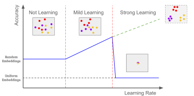
Figure 1: The outcomes of contrastive learning are influenced by the learning rate. A too-small learning rate leads to ineffective embedding transformation, resulting in fine-tuning accuracy reliant on random embeddings. At a medium learning rate, the model learns embeddings more effectively, enhancing accuracy. This is often considered the optimal stage. Conversely, a too-large learning rate causes a significant drop in accuracy, attributed to an overly strong learning effect that converges embeddings to a single point, identified as a local minimum in this study. This paper introduces novel loss terms to counteract this over-fusion phenomenon, thereby harnessing the benefits of strong learning while maintaining stability.

While the effectiveness of these loss functions has been validated across numerous datasets, there is an increasing amount of research indicating instability issue of InfoNCE related methods Yeh et al. (2022); Zhong et al. (2020); Wang et al. (2021); Xie et al. (2022). This instability becomes particularly pronounced with higher learning rates, as illustrated in Figure 1. At moderate learning rates, models tend to start learn embeddings effectively, thereby enhancing accuracy, which is generally considered the optimal learning condition. In contrast, excessively high learning rates lead to a significant drop in accuracy. This is often attributed to an overly aggressive learning effect that causes embeddings to converge prematurely to a singular point. Despite efforts have been made to enhance the InfoNCE loss function, there has been no substantial improvement in accuracy on real-world datasets. In Table 1, we present a summary of the most noteworthy contrastive learning loss functions developed in the last two years. Our analysis reveals that most attempts to improve upon the InfoNCE loss function have either not reached the benchmark accuracy set by InfoNCE or have failed to report accuracy comprehensively. It is noteworthy that only a select few methodologies, markedly diverging from the InfoNCE paradigm, have demonstrated slight improvements in accuracy.

In this study, we undertake a comprehensive analysis of the instability issues in InfoNCE-related loss functions, both empirically and theoretically. We begin with an intuitive 3-dimensional example, where samples are organized within subspace clusters having controlled Gaussian noise. We augment samples by creating negated versions with additional Gaussian noise. Then, we perform self-supervised contrastive learning with a 3-layer Neural Network. During our experiments, a consistent pattern emerged across various loss functions applied to this neural network: a excessive fusion of samples onto a rank-1 linear subspace. This phenomenon of sample fusion could significantly impede the neural network’s performance in later classification tasks. This empirical observation laid the groundwork for our theoretical exploration. We identified a fundamental flaw in the InfoNCE loss function — its inclination to settle into a local minimum, particularly noticeable when samples tend to cluster in a singular, rank-1 subspace. This theoretical insight extends beyond the specific case of InfoNCE, suggesting a broader applicability to all loss functions that are closely related to the InfoNCE scheme.

Expanding on these findings, our study introduces a novel component to contrastive learning, designed for seamless integration with any prevailing loss function. This innovation aims to address and circumvent the issue of the local minima convergence. Central to our approach is the utilization of label information pertinent to the subsequent fine-tuning phase. This involves implementing a regression-like mechanism for the labeled samples of each category, whose targets are orthonormal basis generated randomly at the beginning of training phase. The underlying principle of this strategy is to disentangle the clusters of embeddings for avoiding the problem of over-fusion. Remarkably, our approach requires merely $10\%$ of the labels used in the fine-tuning stage, yet it demonstrates substantial enhancement in performance compared to existing contrastive learning techniques, as evidenced by its application to real-world datasets.

Organization. The structure of the paper is as follows: Section 2 is dedicated to a detailed review of related work in the domain. Next, in Section 3, we delve into both experimental and theoretical analyses to highlight the shortcomings of the InfoNCE approach. Following this, Section 4 introduces our newly proposed loss term, designed to overcome the limitations identified previously. Finally, Section 5 presents a thorough examination of our experimental findings, showcasing the efficacy of our proposed methodology.

2 Backgrounds

A pivotal advancement in the field was presented in the study by Wu et al. (2018) within the realm of unsupervised learning. This research introduced a novel loss function specifically designed for computer vision tasks, which aligns with the contrastive learning framework. Named the Non-Parametric Classifier, this function, also popularly known as InfoNCE, is mathematically expressed as:

$$\mathcal{L}_{\text{infoNCE}}=-\sum_{i\in I}\log\frac{\exp(\mathbf{z}_{i}^{\top}\mathbf{z}_{j(i)}/\tau)}{\sum_{a\neq i}\exp(\mathbf{z}_{i}^{\top}\mathbf{z}_{a}/\tau)}$$ (1)

where $\mathbf{z}_{i}$ signifies the encoder-derived embedding for the i-th sample, and $j(i)$ indicates its corresponding positive pair.

The subsequent section delves into recent innovations in self-supervised contrastive learning, particularly focusing on enhancements to the InfoNCE loss function. These advancements are categorized into three distinct groups: (1) modifications in the components of InfoNCE, including additions or omissions; (2) alterations in the similarity metrics employed within InfoNCE; and (3) other novel approaches that, while not fitting neatly into the aforementioned categories, demonstrate notable improvements in performance. The difference between these methodologies and their experimental results on ImageNet-1K are summarized in Table 1.

Method	Affinity Metric	Aff. to Prob.	Divergence Function	Top-1	Top-5
CPC-v2 Henaff (2020)	Cosine	Softmax	CrossEntropy	71.5	90.1
MOCO-v2 Chen et al. (2020b)	Cosine	Softmax	CrossEntropy	71.1	-
SimCLR Chen et al. (2020a)	Cosine	Softmax	CrossEntropy	69.3	89.0
Inclusion/Removal of Terms within InfoNCE
PCL Cui et al. (2021)	Cosine	Softmax	CrossEntropy	67.6	-
LOOC Xiao et al. (2020)	Cosine	Softmax	CrossEntropy Variant	-	-
DCL Yeh et al. (2022)	Cosine	Decoupled Softmax	CrossEntropy	68.2	-
RC Wang et al. (2022)	Cosine	Softmax	CrossEntropy + L2	61.6	-
Adjustments to the Similarity Function of InfoNCE
Debiased Chuang et al. (2020)	Floor Cosine	Softmax	CrossEntropy	-	-
GCL Koishekenov et al. (2023)	Arccosine	Softmax	CrossEntropy	-	-
HCL Ge et al. (2023)	Cos. + Poincaré	Softmax	CrossEntropy	58.5	-
Innovations
InfoMin Tian et al. (2020b)	Cosine	Softmax	MinMax CrossEntropy	73.0	91.1
VICref Bardes et al. (2021)	Euclidean	NA	Distance + Var + Cov	73.1	91.1
BT Zbontar et al. (2021)	Dimensional Cos.	NA	L2	73.2	91.0

Table 1: Overview of Novel Loss Functions and Baseline Results from 2020: Image Classification Accuracy on ImageNet1K with Unsupervised Learning and Full Label Fine-Tuning. The accuracy measurements are based on training a standard ResNet-50 with 24M parameters. The symbol ’-’ indicates that the corresponding metric was not reported in the original paper.

2.1 Inclusion/Removal of Terms within InfoNCE

Li et al. (2020) introduced an incorporation of the Expectation-Maximization (EM) method into their loss function. Their algorithm employs k-means clustering between each epoch to iteratively update the centroids for each cluster, and use extra terms to minimize mutual information loss between the embeddings and these centroids. Similarly, Wang et al. (2022) introduce an innovative approach designed to extract more valuable information from input images. They achieve this by training a mean function, which is parameterized by a neural network. Their objective is to minimize the infoNCE together with L2 distance between the computed mean and the input picture. The underlying theoretical justification for this method is well-established. However, it’s important to note that in practical experiments, this method yields results that are less competitive compared to the SOTA techniques.

Xiao et al. (2020) introduced a framework that offers support for various combinations of augmentations. This framework aims to reduce the information noise contrastive estimation (infoNCE) by incorporating additional terms designed to enhance the mutual information within images that share similar augmentation components. The formulation seems lack of justification from the paper, and they did not include experimental result from ImageNet1K. Yeh et al. (2022) propose a improvement over infoNCE named Decoupled Contrastive Learning loss(DCL). The core idea behind this formulation is the elimination of a multiplier in the gradients with respect to each variable, resulting in more efficient gradient computation. The authors claim that DCL could improve the original infoNCE on SimCLR and MOCO. However, it is noteworthy that experimental results indicate that DCL performs less favorably when compared to other methods’ accuracy originally claimed.

Input with Aug.	infoNCE	DCL	VICreg	BarlowTwins	Our Method (CLOA)

Table 2: Evaluation of Self-Supervised Contrastive Learning on Synthetic Data with Various Loss Functions. The experiment initiates by generating points from three distinct rank-1 linear subspaces, each perturbed with random Gaussian noise. Subsequent to initialization, these points undergo augmentation through negation and additional Gaussian noise application. A 3-layer feedforward neural network (FFN) model is then trained on this data using several prevalent loss functions until convergence is achieved. Experimental results reveal that conventional loss functions tend to converge to local minima near a rank-1 subspace. Conversely, our proposed loss function significantly mitigates this issue, resulting in the generation of more distinctive and well-separated embeddings.

2.2 Adjustments to the Similarity Function of InfoNCE

Chuang et al. (2020) recognized that when calculating the contrastive learning loss, it’s inappropriate to consider samples belonging to the same class as the anchor image. Consequently, they introduced a function designed to drop the loss if the mean of similarities between negative pairs closely approaches that of the positive pair.

Ge et al. (2023) proposed to treat embeddings as points on hyperbolic space, Poincaré disk specifically. Then, they propose to use the negative geodesic distance as the similarity measurement. Their loss function is then defined as a combination of Euclidean infoNCE and Poincaré infoNCE. Although the idea is innovative, the experimental results yield worse accuracy than SOTA. Similarly, Koishekenov et al. (2023) proposed to use actual angle instead of cosine similarity, but failed to provide any superior performance on ImageNet.

2.3 Innovative Approaches

Tian et al. (2020b) introduced an innovative loss function characterized by a min-max style information-theoretic normalized cross-entropy (infoNCE). Their research yielded intriguing findings, particularly in regard to the influence of data preprocessing on the ultimate classification accuracy. Their result illustrates a pronounced sensitivity in accuracy to both the patch distance within the same image and the parameters used for data augmentation when striving to minimize the infoNCE. Notably, the optimal point lies in the intermediate range, representing a non-trivial balance. They also finds that by training on separate color channels, higher optimal infoNCE leads to better performance for downstream classification.

Bardes et al. (2021) put forth a distinct approach to loss functions. Rather than converting numerical values into probabilities, their method directly employs the Euclidean metric as a fundamental tool. They define the loss as a weighted combination of the Euclidean distance, variance, and covariance. Zbontar et al. (2021) introduce a groundbreaking perspective on leveraging cosine similarity, but with a unique twist applied to different axes of the output matrix. They present a novel loss function that relies on dimension-wise cosine similarity instead of sample-wise similarity. Remarkably, this formulation diverges from conventional infoNCE, especially the classic softmax-crossentropy pair, yet still manages to achieve comparable levels of performance when compared to other methods.

3 Linear Embeddings are Local Minimum

In this section, we aim to establish that linear embeddings represent a local minimum for the majority of contrastive learning loss functions. Our analysis of these losses reveals a critical insight: embeddings confined to a single rank-1 subspace invariably lead to a zero gradient scenario, effectively stalling the learning process. Our exploration begins with synthetic experiments in a three-dimensional setting. Through these, we demonstrate how a model, when trained using self-supervised contrastive learning techniques, can easily falter, resulting in indistinct embeddings.

Following this practical demonstration, we provide a theoretical analysis showing that this vulnerability to generating non-distinctive embeddings is a common shortcoming across most existing contrastive loss functions. This finding highlights a significant concern in the field: the inherent instability of contrastive learning methods. More importantly, it offers valuable insights into the underlying reasons for the frequent failures observed in the learning process.

We begin by initializing three clusters of points within a 3D unit ball, as depicted in the left part of Table 2. These points are assumed to be proximate when they have a small minimum angle between them. This means that even if samples from the same cluster point in nearly opposite directions, they are still considered close as long as the angle between them remains small.

Following this setup, we design a three-layer neural network characterized by dense connectivity, ReLU activation function, and batch normalization. For our training methodology, we adopt the SimpCLR framework Chen et al. (2020a). Each vector is processed by multiplying by $-1$ and adding random Gaussian noise. We repeat this experiments each time starting from random initial conditions and focusing on different loss functions: infoNCE, DCL, VICreg, BarlowTwins. The outcomes of these training sessions are illustrated in the middle and right sections of Table 2.

The results clearly illustrate that the infoNCE regularization imposes a rigid constraint during the learning phase, leading to the convergence of embeddings from distinct classes onto a single line. This results in a representation that lacks sufficient differentiation and expressiveness, a limitation that could be particularly problematic for downstream tasks where the ability to distinguish between various data points is essential. Conversely, methods like VICreg and BarlowTwins, while offering a marginally broader embedding space, still do not adequately separate the three clusters. This minor improvement is consistent with their respective performances on the ImageNet-1K dataset, as detailed in Table 1.

3.1 Theoretical Analysis

This section delves into a theoretical examination of whether linear embeddings constitute local minima for frequently employed contrastive learning loss functions. Initially, we demonstrate that linear embeddings result in a zero gradient scenario specifically for the InfoNCE loss. Subsequently, we extend this discussion to illustrate that this phenomenon is applicable to the vast majority of current, commonly utilized loss functions in contrastive learning. Following this analysis, in Section 4, we introduce our novel loss terms, meticulously designed to address this specific issue.

We first start with InfoNCE, which is still the most common used loss functions for contrastive learning. The loss is defined as:

$$\mathcal{L}_{\text{InfoNCE}}=-\sum_{i\in I}\log\frac{\exp(\mathbf{z}_{i}^{\top}\mathbf{z}_{j(i)}/\tau)}{\sum_{a\notin\{i\}}\exp(\mathbf{z}_{i}^{\top}\mathbf{z}_{a}/\tau)}$$

where $\mathbf{z}_{i}$ represents the embedding generated by the encoder for the i’th sample, and $j(i)$ denotes the positive pair of the sample $i$.

This loss function essentially transforms pairwise similarity scores between embeddings into a probability distribution, subsequently aiming to minimize the information loss relative to a target distribution. The sole interaction with the embeddings involves their comparison against one another. From a broader perspective, if all embeddings are identical, the gradient diminishes to zero due to the absence of angular differences. Moreover, considering that all embeddings are of unit length, an angular difference of $180\degree$ would merely produce a gradient aligned with the current direction of the embeddings. This gradient would then be eliminated during the normalization process. To substantiate this observation with theoretical backing, we present the following Theorem. It shows that with all embeddings being the same or lie in the same line, loss $\mathcal{L}_{\text{InfoNCE}}$ reaches a local minimum with gradient respect to every embeddings equal to zero.

Theorem 3.1.

Let $\mathcal{F}:\mathbb{R}^{m}\to\mathbb{R}^{m^{\prime}}$ be a family of Contrastive Learning structures, where $m$ and $m^{\prime}$ denote the dimensions of the inputs and embeddings, respectively. If a function $f\in\mathcal{F}$ is trained using the InfoNCE loss, then there exist infinitely many local minima where all embeddings produced by $f$ are all equal or lie in the same rank-1 subspace.

The proof of Theorem 3.1 is accomplished by demonstrating that embeddings being equal or in the same rank-1 subspaces, has a zero gradient. Consequently, it establishes it as a local minimum. The detailed proof is available in Appendix A.

4 Our Model: Orthonormal Anchor Regression Loss

To avoid the issue of converging to a single point, we introduce a novel approach that promotes point isolation by adding an additional term to the loss function. Specifically, we utilize the same label set from the fine-tuning phase and incorporate a regression term into the loss function. This term aims to attract known entries towards a specific basis, pre-established before training commences. For entries belonging to different classes, their respective targets are orthogonal. This regression loss acts as a pulling force, preventing the amalgamation of sample groups and, consequently, averting the model from settling into a linear-space local minimum.

Specifically, let $\mathcal{S}$ be a set containing pairs of embeddings and labels, denoted as $\mathcal{S}=\{(\mathbf{z}_{i},y_{i})\mid i\in\{1,\dots,|\mathcal{S}|\}\}$. In addition to the contrastive loss, we introduce a regression loss that maps the embedding $\mathbf{z}_{i}$ to a predefined set of anchors. This set of anchors, denoted as $\mathcal{C}$, is defined as $\mathcal{C}=\{\mathbf{c}_{1},\dots,\mathbf{c}_{k}\}$, where $k$ represents the number of classes in the dataset. Each anchor $\mathbf{c}_{i}$ is initialized as a unit vector orthogonal to all other anchors at the start of the training process. The regression loss is formulated as follows:

$$\mathcal{L}_{\text{CLOA}}=\sum_{i=1}^{|\mathcal{S}|}(1-s(\mathbf{z}_{i},\mathbf{c}_{y_{i}}))$$ (2)

where $s(\cdot,\cdot)$ denotes the distance metric used, commonly chosen as cosine similarity.

The primary objective of our proposed regression loss is to align embeddings corresponding to the same class towards a common target anchor, $\mathbf{c}_{y_{i}}$. This approach is designed to mitigate the issue of over-fusion, where embeddings might converge excessively towards a singular rank-1 subspace. It is important to note that, in the absence of specific constraints, samples external to set $\mathcal{S}$ may still converge to this local minimum, representing a rank-1 subspace. However, a critical assumption in contrastive learning is the treatment of augmented samples as if they are drawn from the same distribution as the original input data. This implies that an augmented version of a sample, say $a$, might exhibit higher similarity to a different sample $b$ than to its own original version. Under this framework, if the label of sample $a$ is observed, and both samples $a$ and $b$ belong to the same class, then sample $b$ is also directed towards the same regression target. This strategic alignment significantly reduces the likelihood of over-fusion, thereby enhancing the efficacy of contrastive learning.

5 Experiment

In the experimental section of this study, we detail our empirical findings, employing CIFAR10 and CIFAR100 with a range of hyper-parameter configurations. Our experiments are grounded in the SimpCLR framework Chen et al. (2020a). Following the recommendations outlined in the original paper, we incorporate ColorJitter with parameters set to brightness=0.2, contrast=0.2, saturation=0.2, and hue=0.1, alongside RandomCrop with a scale ranging from 0.8 to 1.0. Prior to training, all images undergo resizing to dimensions of (3,224,224) and are normalized. The optimization process, both during initial training and subsequent fine-tuning phases, is conducted using Stochastic Gradient Descent (SGD).

Hardware resources utilized for the training tasks include GeForce RTX 2080 Ti and A100-SXM4-40GB GPUs, subject to availability. The duration of our training regimen spans approximately 1100 to 1300 minutes, encompassing 100 epochs of training combined with 100 epochs dedicated to fine-tuning.

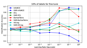
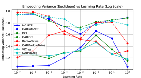
Figure 2: Training results of CIFAR10 on ResNet18 with different learning rates. 10% of labels are used for fine-tuning (50% and 100% trials can be found in Figure 3 in Appendix B). For methods with CLOA loss (dotted lines), we use the same 10% of labels for the regression loss. Top: Top-1 Classification accuracy. Bottom: The variance of embeddings in $\mathbb{R}^{512}$ generated by the backbone encoder. This variance is determined by aggregating the variances across each dimension within the Euclidean space.

5.1 Experiments on CIFAR10

Loss Function	10% Labels	50% Labels	100% Labels
InfoNCE	0.3147	0.4071	0.4382
CLOA-InfoNCE	0.6856	0.6939	0.7009
DCL	0.3514	0.4288	0.4884
CLOA-DCL	0.6521	0.6634	0.6793
BT	0.4148	0.5024	0.5387
CLOA-BT	0.6762	0.6969	0.6995
VICreg	0.4197	0.4674	0.5236
CLOA-VICreg	0.6634	0.6734	0.6908

Table 3: CIFAR10 Classification Accuracy with Different Loss Functions. The table lists the fine-tuning accuracy of the same backbone model using three different percentages of labels (10%, 50%, and 100% respectively). For methods incorporating CLOA loss, a maximum of $10\%$ of labels is utilized for the regression loss. Instances where the accuracy of our method significantly surpasses that of the original method are highlighted for emphasis.

This section details the experiments conducted on the CIFAR10 dataset. For these experiments, the backbone model for all methods is a ResNet18 architecture, which is randomly initialized. A notable modification to the ResNet18 is the removal of its last fully-connected layer. This alteration enables the model to output embeddings of size 512 directly, which are used for training and fine-tuning. During the fine-tuning phase, a feed-forward network with three hidden layers is employed. The dimensions of these layers are set at 256, 128, and 64, respectively, to enhance performance. Throughout the training phase, a consistent batch size of 128 is used, while a batch size of 32 is employed for the fine-tuning phase. Figure 2 shows the training results of different loss functions with different learning rates. The top graph shows the top-1 classification accuracy and the bottom graph shows the variance of embeddings generated from the backbone encoder.

For the original methods that do not include CLOA loss (indicated by solid lines in the figures), a direct correlation is observed between the actual accuracy and the behavior delineated in Figure 1. In particular, with a low learning rate within the range of $[10^{-7},10^{-5}]$, the model remains stagnant in the “Not Learning” phase. As the learning rate increases to between $[10^{-4},10^{-3}]$, the model progresses into the “Mild Learning” phase, leading to a minor enhancement in accuracy. Conversely, a large learning rate within $[10^{-2},10^{0}]$ places the model in the “Strong Learning” phase, resulting in an over-fusion result and the lowest classification accuracy.

The over-fusion phenomenon is further substantiated by the variance graph, depicted at the bottom of Figure 1. In this analysis, the variance of the embeddings in Euclidean space is calculated by aggregating the variance across each dimension. Consequently, it is observed that the variance of embeddings for the original methods demonstrates a marked decrease at higher learning rates. Among the various loss functions, the over-fusion impact is most pronounced with InfoNCE, where the variance sharply falls to nearly zero at a learning rate of 1. This drop in variance correlates with a mere $10\%$ classification accuracy in a 10-class problem. This observation lends credence to the concept of local minima in uniform embeddings, as substantiated in Section 3, given that fine-tuning the classifier for uniform embeddings yields only a $10\%$ accuracy. Moreover, a direct relationship is evident between the variance of embeddings and the ultimate classification accuracy. A majority of the methods attain their peak accuracy when the variance of the embeddings is at its highest, which underscores the significance of embedding diversity in enhancing classification performance.

On the other hand, for methods incorporating CLOA loss (represented as dotted lines in the figures), a distinctly different trend is observed. In these cases, accuracy continually increases even in the “Strong Learning” phase, reaching over twice the original accuracy without any additional use of labels. The efficacy of our loss term in mitigating the over-fusion effect is further substantiated by the behavior of the embedding variance. While the variance initially drops in the “Mild Learning” phase, it notably recovers and increases during the “Strong Learning” phase.

Loss Function	10% Labels		50% Labels		100% Labels
	Top-1	Top-5	Top-1	Top-5	Top-1	Top-5
InfoNCE	0.0279	0.0782	0.0578	0.1005	0.0778	0.1346
CLOA-InfoNCE	0.0238	0.1108	0.0447	0.2401	0.2343	0.3514
DCL	0.022	0.0628	0.0224	0.0977	0.0635	0.1036
CLOA-DCL	0.0246	0.0649	0.0822	0.2013	0.2208	0.3123
BarlowTwins	0.016	0.016	0.0165	0.0165	0.0179	0.0179
CLOA-BarlowTwins	0.0136	0.0543	0.0159	0.0661	0.0531	0.0988
VICreg	0.0332	0.0885	0.0594	0.1084	0.0828	0.1459
CLOA-VICreg	0.0188	0.0825	0.0470	0.1193	0.0589	0.1215

Table 4: CIFAR100 Classification Accuracy with Different Loss Functions. The table lists both the Top-1 and Top-5 fine-tuning accuracies of the same backbone model using three different percentages of labels (10%, 50%, and 100% respectively). For methods incorporating CLOA loss, a maximum of $10\%$ of labels is utilized for the regression loss. Instances where the accuracy of our method significantly surpasses that of the original method are highlighted for emphasis.

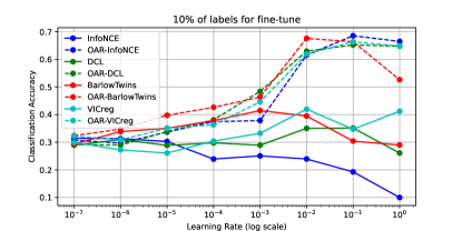
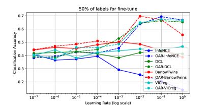
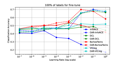
Figure 3: Classification accuracy with different percentage labels for fine-tuning .

Table 3 provides detailed information on the highest classification accuracy achieved using 10%, 50%, and 100% of the labels during the fine-tuning phase. The results for 50% and 100% label usage are additionally illustrated in Figure 3 in Appendix B. In our training processes that incorporate CLOA loss, we exclusively used 10% of the available labels from fine-tuning. This approach led to an increase in accuracy ranging from 25% to 37% when fine-tuning with 10% labels, 19% to 24% when using 50% labels, and 16% to 27% when utilizing 100% labels. Notably, with CLOA, fine-tuning with just 10% of the labels achieves an accuracy within 3% of that achieved using 100% of the labels, demonstrating the effectiveness of our loss term in leveraging limited data for significant accuracy improvements.

5.2 Experiments on CIFAR100

This section details the experiments conducted on the CIFAR100 dataset. For these experiments, a ResNet50 architecture, randomly initialized, is employed as the foundational model across all methods. Echoing the approach used in the CIFAR10 experiments, the ResNet50 is modified by removing its last fully-connected layer. This modification enables the model to directly output embeddings of size 512, facilitating both training and fine-tuning. During the fine-tuning phase, a feed-forward network consisting of three hidden layers is implemented. The dimensions of these layers are strategically set to 512, 1024, and 1024, respectively. In terms of training parameters, a batch size of 128 is utilized for the training phase and a batch size of 32 for the fine-tuning phase. Drawing on insights from the CIFAR10 experiments, the learning rate is set to $10^{-2}$ for original methods and $1$ for methods integrated with CLOA loss. Tables 4 present the top-1 and top-5 classification accuracies achieved using 10%, 50%, and 100% of the labels during the fine-tuning phase.

From the results, it is observed that for 12 out of the 24 reported accuracies, the performance with CLOA loss surpasses that of the original methods by a noticeable margin. In contrast, there is only one instance among these 24 cases where the accuracy employing our loss term is notably lower than that achieved by the original methods. Among the various methods evaluated, the enhancement provided by CLOA loss is particularly pronounced over InfoNCE, DCL, and BarlowTwins. Notably, with just 10% of labels used for fine-tuning, our approach more than doubles the classification accuracy of BarlowTwins. A general improvement in classification accuracies is also observed when full labels are employed for fine-tuning. Overall, the integration of CLOA into the model significantly bolsters its performance, as evidenced by the comparative analysis of the results.

6 Conclusion

In conclusion, our research has successfully addressed a critical challenge in the field of contrastive learning: the instability issues associated with the InfoNCE loss function and its related variants. Our study initially identified a significant limitation in these loss functions, particularly at high learning rates. We observed that such conditions lead to an over-fusion effect, where embeddings are forced to merge into a single point, thereby adversely affecting classification accuracy in downstream tasks.

Through a detailed theoretical analysis, we established that this over-fusion effect represents a local minimum for the InfoNCE loss function. This insight was crucial in guiding our approach to mitigate the issue. Our innovative solution CLOA involves using the same or even fewer labeled data than typically required in the fine-tuning phase, to effectively disentangle embedding clusters. This strategy has proven to be highly effective for improving the performance of the model with large learning rates. Our experiments, conducted on CIFAR10 and CIFAR100 datasets, have demonstrated the efficacy of our approach, marking a substantial improvement over traditional methods in contrastive learning. The success of our methodology not only overcomes a fundamental flaw in prevalent contrastive learning techniques but also opens new avenues for future research in this domain, particularly in scenarios with limited label availability.

Appendix A Proof of Theorem 3.1

Proof of Theorem 3.1.

Consider $\mathcal{L}_{i}$ as the i-th loss term of $\mathcal{L}_{\text{InfoNCE}}$, defined by the following expression:

$$\mathcal{L}_{i}:=-\log\mathbb{P}_{i}$$

where $\mathbb{P}_{i}$ denotes the probability that i-th embedding choose its positive pair as closest neighbor:

$$\mathbb{P}_{i}:=\frac{\exp(\mathbf{z}_{i}^{\top}\mathbf{z}_{j(i)}/\tau)}{\exp(\mathbf{z}_{i}^{\top}\mathbf{z}_{j(i)}/\tau)+\sum_{a\notin\{i,j(i)\}}\exp(\mathbf{z}_{i}^{\top}\mathbf{z}_{a}/\tau)}$$

As detailed in Yeh et al. [2022], the gradient of $\mathcal{L}_{i}$ with respect to $\mathbf{z}_{i}$, $\mathbf{z}_{j(i)}$, and $\mathbf{z}_{a}$ can be derived as follows:

$$-\frac{\partial\mathcal{L}_{i}}{\partial\mathbf{z}_{i}}:=(1-\mathbb{P}_{i})/\tau$$

$$\left(\mathbf{z}_{j(i)}-\sum_{a\notin\{i,j(i)\}}\frac{\exp(\mathbf{z}_{i}^{\top}\mathbf{z}_{a}/\tau)}{\sum_{b\notin\{i,j(i)\}}\exp(\mathbf{z}_{i}^{\top}\mathbf{z}_{b}/\tau)}\mathbf{z}_{a}\right)$$

$$-\frac{\partial\mathcal{L}_{i}}{\partial\mathbf{z}_{j(i)}}:=\frac{(1-\mathbb{P}_{i})}{\tau}\mathbf{z}_{i}$$

$$-\frac{\partial\mathcal{L}_{i}}{\partial\mathbf{z}_{a}}:=-\frac{(1-\mathbb{P}_{i})}{\tau}\frac{\exp(\mathbf{z}_{i}^{\top}\mathbf{z}_{a}/\tau)}{\sum_{b\notin\{i,j(i)\}}\exp(\mathbf{z}_{i}^{\top}\mathbf{z}_{b}/\tau)}\mathbf{z}_{i}$$

In the standard setup of self-supervised learning, for any sample, there is one positive pair among $I$ and the remainder are all negative pairs. By aggregating all the gradient respect to a single sample, we have the gradient of InfoNCE respect to $\mathbf{z}_{i}$:

$$-\frac{\partial\mathcal{L}_{\text{InfoNCE}}}{\partial\mathbf{z}_{i}}:=\frac{(1-\mathbb{P}_{i})+(1-\mathbb{P}_{j(i)})}{\tau}\mathbf{z}_{j(i)}$$

$$-\sum_{a\notin\{i,j(i)\}}\frac{(1-\mathbb{P}_{i})}{\tau}\frac{\exp(\mathbf{z}_{i}^{\top}\mathbf{z}_{a}/\tau)}{\sum_{b\notin\{i,j(i)\}}\exp(\mathbf{z}_{i}^{\top}\mathbf{z}_{b}/\tau)}\mathbf{z}_{a}$$

$$-\sum_{a\notin\{i,j(i)\}}\frac{(1-\mathbb{P}_{a})}{\tau}\frac{\exp(\mathbf{z}_{i}^{\top}\mathbf{z}_{a}/\tau)}{\sum_{b\notin\{a,j(a)\}}\exp(\mathbf{z}_{a}^{\top}\mathbf{z}_{b}/\tau)}\mathbf{z}_{a}$$

Now, considering the first scenario, where all embeddings equal, that means that $\mathbf{z}_{i}=\mathbf{z}_{j(i)}=\mathbf{z}_{a}=\mathbf{z}^{*}$ for all $a\in I$, the loss terms $\mathbb{P}_{i}$, $\mathbb{P}_{j(i)}$, and $\mathbb{P}_{a}$ converge to a constant $\mathbb{P}^{*}$, given by:

$$\mathbb{P}_{i}=\mathbb{P}_{j(i)}=\mathbb{P}_{a}=-\log\frac{1}{|I|-1}:=\mathbb{P}^{*}$$

Consequently, the gradient of $\mathcal{L}_{\text{InfoNCE}}$ with respect to $\mathbf{z}_{i}$ under this assumption reduces to zero, aligning with our expectations:

$$-\frac{\partial\mathcal{L}_{\text{InfoNCE}}}{\partial\mathbf{z}_{i}} =\frac{2(1-\mathbb{P}^{*})}{\tau}\mathbf{z}^{*}-2(|I|-2)\frac{(1-\mathbb{P}^{*})}{\tau}\frac{1}{|I|-2}\mathbf{z}^{*}$$

$$=0$$

We establish the existence of local minima in scenarios where all embeddings are identical. Now, we consider the second scenario where all embeddings generated reside within the same rank-1 subspace. Denoting $\mathbf{z}^{*}$ as their unit basis, we can represent each embedding $\mathbf{z}_{i}$ as:

$$\mathbf{z}_{i}=\alpha\mathbf{z}^{*},\quad\alpha\in\{-1,1\},\quad\forall i$$

The gradient of the loss function $\mathcal{L}_{\text{InfoNCE}}$ with respect to $\mathbf{z}_{i}$ simplifies to:

$$-\frac{\partial\mathcal{L}}{\partial\mathbf{z}_{i}}=\beta\mathbf{z}_{i}$$

Here, $\beta$ is a scalar that aggregates contributions from all relevant weights.

It is important to note that $\mathbf{z}^{i}$ represents the normalized output of the function $f$, with $\tilde{\mathbf{z}}_{i}$ denoting the original, unnormalized embedding. This implies the following relation:

$$-\frac{\partial\mathcal{L}}{\partial\tilde{\mathbf{z}}_{i}} =-\frac{\partial\mathcal{L}}{\partial\mathbf{z}_{i}}\frac{\partial\mathbf{z}_{i}}{\partial\tilde{\mathbf{z}}_{i}}=\frac{1}{\|\mathbf{z}_{i}\|_{2}}\left(\mathbb{I}-\frac{\mathbf{z}_{i}\mathbf{z}_{i}^{\top}}{\mathbf{z}_{i}^{\top}\mathbf{z}_{i}}\right)\beta\mathbf{z}_{i}=0,$$

where $\mathbb{I}$ represents the identity matrix.

∎

Appendix B More CIFAR10 Training Results

References

- Bardes et al. (2021) Adrien Bardes, Jean Ponce, and Yann LeCun. Vicreg: Variance-invariance-covariance regularization for self-supervised learning. arXiv preprint arXiv:2105.04906, 2021.
- Chen et al. (2020a) Ting Chen, Simon Kornblith, Mohammad Norouzi, and Geoffrey Hinton. A simple framework for contrastive learning of visual representations. In International conference on machine learning, pages 1597–1607. PMLR, 2020a.
- Chen et al. (2020b) Xinlei Chen, Haoqi Fan, Ross Girshick, and Kaiming He. Improved baselines with momentum contrastive learning. arXiv preprint arXiv:2003.04297, 2020b.
- Chuang et al. (2020) Ching-Yao Chuang, Joshua Robinson, Yen-Chen Lin, Antonio Torralba, and Stefanie Jegelka. Debiased contrastive learning. Advances in neural information processing systems, 33:8765–8775, 2020.
- Cui et al. (2021) Jiequan Cui, Zhisheng Zhong, Shu Liu, Bei Yu, and Jiaya Jia. Parametric contrastive learning. In Proceedings of the IEEE/CVF international conference on computer vision, pages 715–724, 2021.
- Ge et al. (2023) Songwei Ge, Shlok Mishra, Simon Kornblith, Chun-Liang Li, and David Jacobs. Hyperbolic contrastive learning for visual representations beyond objects. In Proceedings of the IEEE/CVF Conference on Computer Vision and Pattern Recognition, pages 6840–6849, 2023.
- Henaff (2020) Olivier Henaff. Data-efficient image recognition with contrastive predictive coding. In International conference on machine learning, pages 4182–4192. PMLR, 2020.
- Jaiswal et al. (2020) Ashish Jaiswal, Ashwin Ramesh Babu, Mohammad Zaki Zadeh, Debapriya Banerjee, and Fillia Makedon. A survey on contrastive self-supervised learning. Technologies, 9(1):2, 2020.
- Koishekenov et al. (2023) Yeskendir Koishekenov, Sharvaree Vadgama, Riccardo Valperga, and Erik J Bekkers. Geometric contrastive learning. In Proceedings of the IEEE/CVF International Conference on Computer Vision, pages 206–215, 2023.
- Li et al. (2020) Junnan Li, Pan Zhou, Caiming Xiong, and Steven CH Hoi. Prototypical contrastive learning of unsupervised representations. arXiv preprint arXiv:2005.04966, 2020.
- Tian et al. (2020a) Yonglong Tian, Dilip Krishnan, and Phillip Isola. Contrastive multiview coding. In Computer Vision–ECCV 2020: 16th European Conference, Glasgow, UK, August 23–28, 2020, Proceedings, Part XI 16, pages 776–794. Springer, 2020a.
- Tian et al. (2020b) Yonglong Tian, Chen Sun, Ben Poole, Dilip Krishnan, Cordelia Schmid, and Phillip Isola. What makes for good views for contrastive learning? Advances in neural information processing systems, 33:6827–6839, 2020b.
- Wang et al. (2022) Haoqing Wang, Xun Guo, Zhi-Hong Deng, and Yan Lu. Rethinking minimal sufficient representation in contrastive learning. In Proceedings of the IEEE/CVF Conference on Computer Vision and Pattern Recognition, pages 16041–16050, 2022.
- Wang et al. (2021) Xudong Wang, Ziwei Liu, and Stella X Yu. Unsupervised feature learning by cross-level instance-group discrimination. In Proceedings of the IEEE/CVF conference on computer vision and pattern recognition, pages 12586–12595, 2021.
- Wu et al. (2018) Zhirong Wu, Yuanjun Xiong, Stella X Yu, and Dahua Lin. Unsupervised feature learning via non-parametric instance discrimination. In Proceedings of the IEEE conference on computer vision and pattern recognition, pages 3733–3742, 2018.
- Xiao et al. (2020) Tete Xiao, Xiaolong Wang, Alexei A Efros, and Trevor Darrell. What should not be contrastive in contrastive learning. arXiv preprint arXiv:2008.05659, 2020.
- Xie et al. (2022) Yutao Xie, Qiyu Wu, Wei Chen, and Tengjiao Wang. Stable contrastive learning for self-supervised sentence embeddings with pseudo-siamese mutual learning. IEEE/ACM Transactions on Audio, Speech, and Language Processing, 30:3046–3059, 2022.
- Yeh et al. (2022) Chun-Hsiao Yeh, Cheng-Yao Hong, Yen-Chi Hsu, Tyng-Luh Liu, Yubei Chen, and Yann LeCun. Decoupled contrastive learning. In European Conference on Computer Vision, pages 668–684. Springer, 2022.
- Zbontar et al. (2021) Jure Zbontar, Li Jing, Ishan Misra, Yann LeCun, and Stéphane Deny. Barlow twins: Self-supervised learning via redundancy reduction. In International Conference on Machine Learning, pages 12310–12320. PMLR, 2021.
- Zhong et al. (2020) Huasong Zhong, Chong Chen, Zhongming Jin, and Xian-Sheng Hua. Deep robust clustering by contrastive learning. arXiv preprint arXiv:2008.03030, 2020.