Globally integrable quantum systems and their perturbations

Abstract

In this paper we present the notion of globally integrable quantum system that we introduced in [BL22]: we motivate it using the spectral theory of pseudodifferential operators and then we give some results on linear and nonlinear perturbations of a globally integrable quantum system. In particular, we give a spectral result ensuring stability of most of its eigenvalues under relatively bounded perturbations, and two results controlling the growth of Sobolev norms when it is subject either to linear unbounded time dependent perturbations or a small nonlinear Hamiltonian nonlinear perturbation.

Keywords: Schrödinger operator, normal form, Nekhoroshev theorem, pseudo differential operators

MSC 2010: 37K10, 35Q55

1 Introduction

In this paper we review some results that we recently got on perturbations of “globally integrable quantum systems”.

One of the key points is the definition of globally integrable quantum system. Indeed, as far as we know, there is not a generally accepted definition of integrable quantum system, thus in the first part of the paper (see Sections 2, 3, 4, 5) we first motivate and then give our definition of globally integrable quantum system (GIQS). Roughly speaking, a GIQS is a Hamiltonian operator which is a function of the quantum actions. In turn we define the quantum actions to be a set of commuting self-adjoint operators with pure point spectrum contained in $\mathbb{Z}+\kappa$, where $\kappa\in\mathbb{R}$ is a real number.

The main feature of GIQS is that, on the one hand (as showed by the result presented in Section 6) they have very strong stability properties when perturbed, and on the other hand it turns out that they cover several nontrivial examples. That is the reason why we think they are of interest.

GQIS exhibit stability properties both from the spectral point of view and from a dynamical point of view, when the Schrödinger equation relative to a GIQS is perturbed by a relatively bounded family of time dependent pseudodifferential operators, or by a small nonlinear Hamiltonian perturbation.

Such results are reviewed respectively in the Subsections 6.1 and 6.2. Subsection 6.1 is split in a paragraph dealing with the spectral problem and a paragraph dealing with the dynamical problem. In Paragraph 6.1.1 we present the spectral result, according to which most of the eigenvalues of a perturbation of a GIQS admit an asymptotic expansion in inverse powers of their size. In Paragraph 6.1.2 we state the result on time dependent perturbations of the Schrödinger equation, according to which the Sobolev norms of the solution are bounded by $|t|^{\epsilon}$ for all $\epsilon>0$.

Then, in Subsection 6.2 we study a nonlinear Hamiltonian PDE which is a perturbation of the Schödinger equation with unperturbed Hamiltonian given by a GIQS. Here we give an almost global existence result, namely we prove that for initial data with Sobolev norm of order $\epsilon$ the Sobolev norm of the corresponding solution remains of order $\epsilon$ for times of order $\epsilon^{-N}$, $\forall N$. We also give a couple of applications to concrete nonlinear PDEs.

The main tool for the proof of all the abstract results is a clustering property of the spectrum of a GIQS. Such a clustering is described in Section 7 and is constructed by quantizing the so called geometric part of the proof of classical Nekhoroshev’s theorem. Such a clustering has also a property that was identified by Bourgain as a key property for the proof of KAM type results in PDEs. For this reason we call it Nekhoroshev-Bourgain partition.

In Section 7 we also give a qualitative description of the way the clustering is used in order to prove the results presented in Section 6.

We close this introduction by recalling that in the line of research of this paper one finds a very extensive literature. In particular we recall that this line of research on the quantization of classical perturbation theory was initiated many years ago, in particular we recall [DS96, DLSV02, Com88, Bel85, BG01], and more recent developments were obtained in [Bam18, Bam17, BM18] for 1-d systems and [BGMR18, BGMR21] for some higher dimensional systems. Then we investigated the case of a nontrivial unperturbed structure of the resonance relations in [BLM20, BLM22b, BLM22a, BL22].

The case of nonlinear Hamiltonian with semilinear perturbations originated from the papers [Bam03, BG06] for 1-d systems, the case of the wave equation on Zoll manifolds was studied in [BDGS05] (see also [BG03, GIP09]). Recently such a theory was extended to the case of quasilinear perturbations [BD18, BMM22]. The case of general tori was dealt with in [BFM24], which was also the starting point of our work [BFLM24]. We also recall the paper [DI17], which had a strong influence on our result [BFLM24].

Acknowledgments The authors would like to thank Francesco Fassò for interesting explanations on superintegrable systems and Giorgio Gubbiotti for a discussion on quantum integrable systems. This project is supported by INDAM and by PRIN 2020 (2020XB3EFL001) “Hamiltonian and dispersive PDEs”.

2 Classical Integrable and Superintegrable Systems.

Let $M$ be an $n$ dimensional Riemannian manifold, and consider the symplectic manifold given by the cotangent boundle $T^{*}M$. Let $h\in C^{\infty}(T^{*}M)$ be a Hamiltonian function. Then to $h$ one associates the corresponding Hamiltonian vector field $X_{h}$ defined by $\omega_{z}(X_{h}(z),k)=dh(z)k$, $\forall k\in T_{z}(T^{*}M)$, where $\omega_{z}$ is the symplectic form at $z\in T^{*}M$. It is well known that in any canonical coordinate system of $T^{*}M$ the Hamilton equations $\dot{z}=X_{h}(z)$ take the form

$$\dot{\xi}=-\partial_{x}h\ ,\quad\dot{x}=\partial_{\xi}h\ .$$

In this case $n=dim(M)$ is called the number of degrees of freedom of the Hamiltonian system $h$.

One also defines the Poisson Brackets of two functions by

$$\left\{f_{1};f_{2}\right\}:=df_{1}X_{f_{2}}\ .$$

2.1 Integrable systems

Definition 2.1.

Let $f_{1},...,f_{k}\in C^{\infty}(T^{*}M)$ be $k$ smooth functions. They are said to be independent if the covectors

$$df_{1}(z),...,df_{k}(z)$$

are independent for almost every $z$.

The functions are said to be in involution if

$$\left\{f_{j};f_{j}\right\}=0\ ,\forall i,j=1,...,k\ .$$

It is well known that the maximal number of functions which are independent and in involution in a manifold of dimension $n$ is $n$.

Definition 2.2.

A Classical Hamiltonian system is said to be integrable if it admits $n$ prime integrals which are independent and in involution, namely if there exist $f_{1},...,f_{n}$ independent and in involution and s.t. $\left\{h;f_{j}\right\}\equiv 0$.

It is well known that the main result of classical integrable systems is the so called Arnold Liouville theorem, which can be stated as follows

Theorem 2.3.

Let $h$ be an integrable system; let $z_{0}\in T^{*}M$ be s.t. the differentials $df_{j}(z_{0})$ are independent and denote $m_{j}=f_{j}(z_{0})$. If the level surface

$$S_{0}:=\left\{z\in T^{*}M\ :\ f_{j}(z)=m_{j}\quad\forall j=1,\dots,n\right\}$$

is compact, then $S_{0}$ is diffeomorphic to an $n$ dimensional torus and there exists a neighborhood ${\mathcal{U}}$ of $S_{0}$ foliated in invariant $n$ dimensional tori. Furthermore there exist ${\mathcal{A}}\subseteq\mathbb{R}^{n}$ and a symplectic coordinate system $(a,\alpha):{\mathcal{A}}\times\mathbb{T}^{n}\to{\mathcal{U}}$, with the property that in such coordinates $h$ is a function of $a$ only.

The coordinates $(a,\alpha)$ are called Action Angle coordinates.

Remark 2.4.

For the extension to quantum systems, the main property of the action coordinates is that the coordinate canonically conjugated to each $a_{j}$ is an angle. This means that if one considers the Hamiltonian given by the action $a_{j}$, such a Hamiltonian generates a flow which is periodic of period $2\pi$.

Our main goal is to define the quantum analogue of the action variable, which in principle is just the operator obtained by quantizing the classical action. However, quantization is an easy procedure only for globally defined functions: for this reason we are particularly interested in situations in which the action variables do not have singularites, or have only singularities which can be eliminated.

Remark 2.5.

In this paper, we are interested in the behavior of functions at infinity. For this reason, the possibly harmful singularities are only those accumulating at infinity. A typical example are the circular orbits of the central motion problem, in which the effective radial Hamiltonian has critical points. It will turn out that such critical points can be regularized quite easily if they are elliptic, while the hyperbolic case is not covered by the theory developed here. We also remark that in more general cases one can meet also singularities of focus-focus kind, whose semiclassical theory has been developed by [PVN14].

2.2 Superintegrable systems

A further interesting case where the set of action angle variables is singular is the case of superintegrable Hamiltonian system, however in such a case one has that some of the action variables are typically globally defined and furthermore the Hamiltonian only depends on these globally defined action variables, a phenomenon which is also related to Gordon’s theorem [Gor70, Nek05]. As a consequence our theory will turn out to be applicable also to several superintegrable systems.

We recall that in the case of superintegrable systems the geometry of the phase space is described “semiglobally” by a classical theorem by Nekhoroshev [Nek72] (see also [Fas05] and literature cited therein). We will not state the corresponding theorem, instead we are going to describe the situation in the case of a free particle on the 2 dimensional sphere.

So, consider a particle on the two dimensional sphere, which is a system with two degrees of freedom. Here there exist three independent integrals of motion which are the three components of the angular momentum. From these variables one can extract two integrals of motion which are independent and in involution, namely the $z$ component ${\tt M}_{z}$ of the angular momentum and the square ${\tt M}^{2}$ of the total angular momentum. A system of action coordinates is given by ${\tt M}$ and by ${\tt M}_{z}$. The corresponding angles can then be constructed by the standard procedure obtaining a system of action angle variables.

Such a system of coordinates has a singularity when (1) the total angular momentum is in the direction of the $z$ axis, since here the two actions are no more independent and (2) when the total angular momentum vanishes. However, it is clear that the first singularity is just related to the choice of the $z$ axis and that the other action ${\tt M}$ is smooth at such a singularity, while at ${\tt M}=0$, there is a singularity of the action variable, but the Hamiltonian, which is a function just of ${\tt M}^{2}$ is smooth also at ${\tt M}=0$.

This is the typical semiglobal situation described by Nekhoroshev’s theorem [Nek72]: one of the actions is defined on a whole neighborhood of a level surface of the integrals of motion, while the other one is not. Typically, a neighborhood ${\mathcal{U}}$ of the level surface has the structure of a bi-fibration ${\mathcal{U}}\to^{1}{\mathcal{B}}\to^{2}{\mathcal{A}}\subset\mathbb{R}$, where ${\mathcal{A}}$ is the domain of the true action on which the Hamiltonian depends, the fibers of the first map $1$ are one dimensional tori, while the fibers of the second fibration $2$ are typically compact surfaces. In the case of the free motion on the sphere, they are locally the product of a two dimensional sphere and a 1 dimensional torus. Actually the topological structure of the two dimensional sphere is the reason why the third action is not globally defined.

2.3 Conclusion

As a conclusion of this section, we just summarize that classical integrable systems are systems in which locally the Hamiltonian is a function of the action variables. In turn, the action variables are functions on the phase space which, when used as Hamiltonian, generate a flow which is periodic with period $2\pi$.

Typically the action variables are only defined locally in the phase space, but there are situations in which they are defined globally.

A particular situation is that of superintegrable systems, in which the Hamiltonian only depends on a number of actions smaller than the number of degrees of freedom, and in some interesting situations such actions are globally defined.

This is a first set of considerations that we use as a basis for the definition of quantum actions and quantum integrable system that we will give in Section 5.1.

3 Quantizing Hamiltonians with periodic flow

As observed in Remark 2.4 and Subsect. 2.3, the actions of an integrable system generate a periodic Hamiltonian flow. With this in mind, in this section we discuss quantum operators obtained by quantizing a Hamiltonian whose flow is periodic. We will carry on in a parallel way the theory on on $\mathbb{R}^{n}$ and on compact manifolds.

To start with consider the case of $\mathbb{R}^{n}$, where the phase space is $T^{*}\mathbb{R}^{n}\simeq\mathbb{R}^{n}\times\mathbb{R}^{n}$. We follow the theory developed by Helffer-Robert in [HR82], which is adapted to the study of anharmonic oscillators in $\mathbb{R}^{n}$, namely the systems with classical Hamiltonian

$$h_{An}(x,\xi):=\frac{\left\|\xi\right\|^{2}}{2}+\frac{\left\|x\right\|^{2\ell}}{2\ell}\ ,\quad\ell\in\mathbb{N}^{*}\ .$$ (3.1)

In order to precisely state the result in [HR82], we need to introduce some setting. First we introduce a scale of Hilbert spaces $\{{\mathcal{H}}_{An}^{s}\}_{s\geq 0}$ adapted to this situation by defining the operator $K^{(0)}_{An}:=(-\Delta+\|x\|^{2\ell})^{\frac{\ell+1}{2\ell}}$ and putting, for $s\geq 0$ ${\mathcal{H}}_{An}^{s}:=D([K_{0}^{(s)}]^{s})$ endowed by the graph norm. For $s<0$ we also define ${\mathcal{H}}_{An}^{s}$ to be the dual to ${\mathcal{H}}_{An}^{-s}$ with respect to the $L^{2}$ scalar product.

We also need to introduce the concept of a quasihomogeneous function.

Definition 3.1.

Fix $\ell\in\mathbb{N}$, then a function $a\in C^{\infty}(\mathbb{R}^{2n}\setminus\{0\})$ is said to be quasihomogeneous of degree $m\in\mathbb{R}$ if

$$a\left(\lambda^{\frac{1}{\ell+1}}x,\lambda^{\frac{\ell}{\ell+1}}\xi\right)=\lambda^{m}a(x,\xi)\quad\forall\lambda\in\mathbb{R}^{+}\,,\quad\forall(x,\xi)\in\mathbb{R}^{2n}\ .$$ (3.2)

Then we define also a class of symbols adapted to this situation: denote

$${\tt k}_{0}(x,\xi):=(1+\|x\|^{2\ell}+\|\xi\|^{2})^{\frac{1+\ell}{2\ell}}\ .$$

Definition 3.2.

A function $f$ will be called a symbol of order $m\in\mathbb{R}$ if $f\in C^{\infty}(\mathbb{R}^{n}_{x}\times\mathbb{R}^{n}_{\xi})$ and $\forall\alpha,\beta\in\mathbb{N}^{n}$, there exists $C_{\alpha,\beta}>0$ s.t.

$$|\partial_{x}^{\alpha}\,\partial_{\xi}^{\beta}f(x,\xi)|\leq C_{\alpha,\beta}\ {\tt k}_{0}(x,\xi)^{m-\frac{\ell|\beta|+|\alpha|}{1+\ell}}\ .$$ (3.3)

We will write $f\in S^{m}_{An}$.

To a symbol $f\in S^{m}_{An}$ we associate the operator $F\equiv Op^{W}(f)$ which is obtained by standard Weyl quantization, namely

$$(Fu)(x):=\frac{1}{(2\pi)^{n}}\int_{\mathbb{R}^{n}}\int_{\mathbb{R}^{n}}e^{{\rm i}\langle x-\eta,\xi\rangle}f\left(\frac{x+\eta}{2},\xi\right)u(\eta)\,d\eta\ d\xi\,.$$ (3.4)

Definition 3.3.

We say that $F$ is a pseudodifferential operator of order $M$ and we write $F\in\operatorname{OPS}_{An}^{m}$ if there exist $f\in S^{m}_{An}$ and a smoothing operator $S$ such that $F=Op^{W}(f)+S$. Here by smoothing operator we mean an operator $S$ mapping ${\mathcal{H}}_{An}^{s}$ into ${\mathcal{H}}_{An}^{s+N}$ for any $s$ and any $N>0$.

In this framework we have the following theorem:

Theorem 3.4.

[Helffer-Robert, [HR82]] Let $a\in S^{1}_{An}$ be quasihomogeneous of degree 1 and assume that all the solutions of the corresponding Hamilton equations are periodic with period $2\pi$. Assume also that the corresponding Weyl operator $A$ is positive definite, then there exist an operator $Q\in\operatorname{OPS}_{An}^{-1}$ commuting with $A$ and $\kappa\in\mathbb{R}$ s.t.

$$\sigma(A+Q)\subset\mathbb{Z}+\kappa\ .$$ (3.5)

By $\sigma(A)$ we are denoting the spectrum of the operator $A$.

Figure 1: Representation of the path $\gamma$.

Idea of the proof. The idea is first to prove that

$$\exp\left(-2\pi{\rm i}\left(A-\kappa\right)\right)={\bf 1}+C\,,$$ (3.6)

with some $C\in\operatorname{OPS}_{An}^{-1}$ and then to pass to the logarithm. The intuition is that, by Egorov’s theorem, one has that, for any pseudodifferential operator $B$ one has

$$\exp\left(-2\pi{\rm i}A\right)B\exp\left(2\pi{\rm i}A\right)=B+l.o.t.$$ (3.7)

so that, one expects that, up to lower order terms, $\exp\left(-2\pi{\rm i}A\right)$ is a purely imaginary constant.

The actual proof is slightly different: we are now going to summarize how it works. Consider again the operator $U(2\pi):=\exp(-{\rm i}2\pi A)$. The first step consists in exploiting Egorov theorem (3.7) in order to show that, since the classical flow of $a$ is periodic, $U(2\pi)$ satisfies Beals’ characterization [Bea77] and therefore it is a pseudodifferential operator in a suitable class. Then one has to study the principal symbol $u_{2\pi}$ of $U(2\pi)$. First one gets that it is quasihomogeneous of degree 0. Then one has to show that it is constant. To this end one defines a quasihomogeneous function

$$M(x,\xi):=\lim_{\lambda\to\infty}u_{2\pi}(\lambda^{2}x;\lambda^{2\ell}\xi)\ ,$$

which is easily seen to exist everywhere and finally one proves that such a function is actually independent of $(x,\xi)$. This last step is done by writing $u_{T}(\lambda^{2}x,\lambda^{2\ell}\xi)$ as the integral of its differential along the curve

$$t\mapsto((\lambda t)^{2}x,(\lambda t)^{2\ell}\xi)\,,\quad t\in[0,1]\,,$$ (3.8)

and then by studying the integral of the differential of $u_{T}$ on the closed curve $\gamma$ constructed as in Figure 1. In particular, given $\varepsilon$ and $\lambda>0$, one takes two points $(x,\xi)$, $(x^{\prime},\xi^{\prime})$ on the ellipse $x^{2}+\xi^{\frac{2}{2\ell}}=\varepsilon^{2}$. Then the support of $\gamma$ is built as

$$\operatorname{\gamma}=\Gamma_{\varepsilon}\cup\Delta_{\varepsilon,\lambda}\cup\Gamma_{\lambda}\cup\Delta^{\prime}_{\varepsilon,\lambda}\,,$$

where

• $\Gamma_{\varepsilon}$ is the shortest arc of the ellipse joining $(x,\xi)$ and $(x^{\prime},\xi^{\prime})$

• $\Delta_{\varepsilon,\lambda}$ is the arc of the curve (3.8) joining $(x,\xi)$ with $(\lambda^{2}x,\lambda^{2\ell}\xi)$

• $\Delta^{\prime}_{\varepsilon,\lambda}$ is constructed as $\Delta_{\varepsilon,\lambda}$ but replacing $(x,\xi)$ with $(x^{\prime},\xi^{\prime})$

• $\Gamma_{\lambda}$ is the arc of ellipse joining $(\lambda^{2}x,\lambda^{2\ell}\xi)$ with $(\lambda^{2}x^{\prime},\lambda^{2\ell}\xi^{\prime})$.

Then one proves that, as $\varepsilon\rightarrow 0$ and $\lambda\rightarrow\infty$, the integrals on $\Gamma_{\varepsilon}$ and on $\Gamma_{\lambda}$ tend to $0$. Thus, one gets that the two integrals on $\Delta_{\varepsilon,\lambda}$ and on $\Delta_{\varepsilon^{\prime},\lambda^{\prime}}$ coincide in the limit $\varepsilon\rightarrow 0$ $\lambda\rightarrow\infty$, namely $M(x,\xi)=M(x^{\prime},\xi^{\prime})$. Finally, since $U$ is unitary, one must have $|M|=1$, and this allows to conclude the proof. ∎

The above theorem clarifies the situation in the case of operators on $\mathbb{R}^{n}$. We come now to the case of compact manifolds. So, let $M$ be a compact Riemannian manifold and denote by $\Psi^{m}(M)$ the space of pseudodifferential operators of order $m$ à la Hörmander (see [Hö85], Chapter 18 for the precise definition). First we recall that a function $a\in C^{\infty}(T^{*}M\setminus\{0\})$ is homogeneous of degree m, if in any canonical coordinate system on $T^{*}M$ it has the property that

$$a(x,\lambda\xi)=\lambda^{m}a(x,\xi)\ ,\ \forall\lambda>0\ .$$

The analogue of Theorem 3.4 for the case of compact manifolds is the following theorem:

Theorem 3.5.

[Theorem 1.1 of [CDV79]] Let $a\in C^{\infty}(T^{*}M\setminus\{0\})$ be homogeneous of degree 1 and denote by $A$ its Weyl quantization; assume that all the orbits of the Hamiltonian vector field of $a$ are periodic with period $2\pi$, then there exists a pseudodifferential operator $Q\in\Psi^{-1}(M)$ of order $-1$, which commutes with $A$ and a real number $\kappa$ s.t.

$$\sigma(A+Q)\subset(\mathbb{Z}+\kappa)\ .$$ (3.9)

Namely, up to a correction smoothing of order $-1$ the quantization of a Hamiltonian with periodic flow has spectrum contained in a translation of $\mathbb{Z}$.

3.1 Conclusion

Both in the case of $\mathbb{R}^{n}$ and in the case of compact manifolds, the quantization of a globally defined action is an operator $A$ with the property that there exists an operator $Q$ of order $-1$, which commutes with $A$ and has spectrum contained in a translation of $\mathbb{Z}$.

Thus the idea that one can consider is to neglect the regularizing perturbation and to define directly a quantum action to be a pseudodifferential operator of order 1 with spectrum contained in a translation of $\mathbb{Z}$. As shown in the next section, this has the advantage that in some situations one can avoid to pass through the classical system.

4 Two purely quantum examples

In this section we give two examples of quantum models where the Hamiltonian can be described as a function of a few number of operators $A_{1},\dots,A_{\mathtt{d}}$, each of which has spectrum lying on $\mathbb{Z}+\kappa_{j}$ for a suitable real $\kappa_{j}$.

The first simple example is that of a free quantum particle on the $d$ dimensional sphere, whose Hamiltonian is the Laplace-Beltrami operator on the sphere. In this case it is well known that the spectrum of the Laplacian is given by $j(j+(n-1))$, and the corresponding eigenspace is spanned by the spherical Harmonics $Y_{j,l}$. Thus in particular one can write $-\Delta_{g}=(A+Q)^{2}$, with $A$ defined by

$$AY_{j,l}:=\left(j+\frac{n-1}{2}\right)Y_{j,l}\ ,$$

and $Q$ defined as a spectral multiplier of order $-1$.

So, in this case one can define a quantum action to be the operator $A$ and the Laplace-Beltrami operator turns out to be a bounded perturbation of $A^{2}$.

The situation is similar on Zoll manifolds, on which one still has $-\Delta_{g}=(A+Q)^{2}$ and $Q$ is a pseudodifferential operator of order $-1$.

A second quantum example is that of a free quantum particle on a simply connected compact Lie group $G$. We remark that in the case of $M=SO(3)$ this is a quantum rigid body. Endow $M$ by the bi-invariant metric, which in the case of the rigid body corresponds to the case of a spherically symmetric rigid body. The corresponding (quantum) Hamiltonian is the Laplace-Beltrami operator $-\Delta_{g}$. As we will show in a while, in this case the Laplacian turns out to be the function of a few number of operators with spectrum lying on $\mathbb{Z}+\kappa$, for some $\kappa\in\mathbb{R}$.

To describe this point we have to rapidly introduce the intrinsic Fourier series on Lie groups. The key point is that the Fourier coefficients of a function on a Lie group are labeled by the irreducible unitary representations of $G$. More precisely, if $\xi$ is an irreducible unitary representation, then the corresponding Fourier coefficient of a function $\psi$ is an element of the representation space of such a representation (see for instance [Pro07]). Furthermore one has that such representations are in 1-1 correspondence with the elements of the cone $\Lambda^{+}(G)$ of the dominant weights, defined by

$$\Lambda^{+}(G)=\left\{{\tt w}\in\mathbb{R}^{d}\ \left|\ {\tt w}={\tt w}^{1}{\tt f}_{1}+\dots+{\tt w}^{d}{\tt f}_{d}\,,\quad{\tt w}^{j}\in\mathbb{N}\ ,\ \forall j=1,\dots,d\right.\right\}\,,$$ (4.1)

where ${\tt f}_{1},\dots,{\tt f}_{d}\in\mathbb{R}^{d}$ are the fundamental weights of $G$. In this language the Laplacian is a Fourier multiplier. Precisely, given a dominant weight, ${\tt w}$ consider its decomposition on the basis ${\tt f}_{j}$, namely ${\tt w}=\sum_{j=1}^{d}{\tt w}^{j}{\tt f}_{j}$, then the Laplacian is the Fourier multiplier by

$$\sum_{j,i}({\tt w}^{j}+1)({\tt w}^{i}+1){\tt f}_{i}\cdot{\tt f}_{j}-\sum_{j,i}{\tt f}_{i}\cdot{\tt f}_{j}\ ,$$

which is a homogeneous quadratic function of the basic Fourier multipliers

$$A_{j}:=\text{multiplier\ by}\ ({\tt w}^{j}+1)\ .$$ (4.2)

Remark 4.1.

Since ${\tt w}^{j}$ are integers, the spectrum of such operators are just contained in $\mathbb{Z}$. Furthermore, exploiting the results of [Fis15], in [BL22] we proved that such operators are actually pseudodifferential operators in the sense of Hörmander.

Actually it can be seen that the situation is absolutely similar in homogeneous spaces. We also remark that the sphere is also a homogeneous space, and this suggests that there should be a connection between the two examples of this section. However, we also remark that Zoll manifolds are not, in general, homogeneous spaces.

5 Globally integrable quantum systems

The theorems and the examples of the previous sections give a strong hint on a possible definition of quantum action and quantum integrable system.

We will treat in a unified way both the situation of a compact manifold or that of $\mathbb{R}^{n}$. In particular on $\mathbb{R}^{n}$ we are interested to the anharmonic oscillator with quantum Hamiltonian

$$H_{An}:=-\frac{\Delta}{2}+\frac{\left\|x\right\|^{2\ell}}{2\ell}\ ,$$ (5.1)

with some fixed $\ell\in\mathbb{N}$, $\ell\geq 1$. We define

$$K_{0}:=\left\{\begin{matrix}({\bf 1}-\Delta_{g})^{1/2}\ &\text{if }&M&\text{is\ compact}\\ ({\bf 1}+H_{An})^{(\ell+1)/2\ell}\ &\text{if }&M&\text{is}\ \mathbb{R}^{n}\end{matrix}\right.\,.$$ (5.2)

Then we consider the scale of Hilbert spaces ${\mathcal{H}}^{s}:=D(K_{0}^{s})$, if $s>0$ and ${\mathcal{H}}^{s}$ the dual of ${\mathcal{H}}^{-s}$ with respect to the $L^{2}$ scalar product, if $s<0$.

Concerning pseudodifferential operators, we define

$${\mathcal{A}}^{m}:=\left\{\begin{matrix}\Psi^{m}(M)\ &\text{if }&M&\text{is\ compact}\\ \operatorname{OPS}_{An}^{m}\ &\text{if }&M&\text{is}\ \mathbb{R}^{n}\end{matrix}\right.$$ (5.3)

5.1 Definitions

As anticipated above, the actions will be a set of commuting self-adjoint operators, each of which with spectrum contained in a translation of $\mathbb{Z}$.

Before giving the precise definition we recall that, given a set of self-adjoint operators $A_{1},...,A_{d}$ with pure point spectrum, their joint spectrum is defined as follows:

Definition 5.1.

The joint spectrum $\Lambda$ of the operators $A_{j}$ is the set of the ${a=(a^{1},\dots,a^{d})}\in\mathbb{R}^{d}$ s.t. there exists $\psi\in{\mathcal{H}}$ with

$$A_{j}\psi=a^{j}\psi\ ,\quad\forall j=1,...,d\ .$$ (5.4)

Definition 5.2 (Set of quantum actions).

A set of self-adjoint pseudodifferential operators $(A_{1},...,A_{d})$, with $A_{j}\in{\mathcal{A}}^{1}$ are said to be a set of quantum actions if

• They are pairwise commuting

• $\exists c_{1}>0$ s.t. $c_{1}K_{0}^{2}<{\bf 1}+\sum_{j=0}^{d}A_{j}^{2}$.

• There exist a convex closed cone ${\mathcal{C}}\subseteq\mathbb{R}^{d}$ and a vector $\kappa=(\kappa_{1},...,\kappa_{d})\in\mathbb{R}^{d}$, such that the joint spectrum $\Lambda$ of the $A_{j}$’s fulfills

  $$\Lambda\subset(\mathbb{Z}^{d}+\kappa)\cap{\mathcal{C}}\ .$$ (5.5)

Definition 5.3.

A self-adjoint operator $H_{L}$ is said to be globally integrable if there exists a function $h_{L}:\mathbb{R}^{d}\to\mathbb{R}$ with the property that

$$H_{L}=h_{L}(A_{1},...,A_{d})\ ,$$ (5.6)

with the operator function spectrally defined.

We remark that Definition 5.3 is given in order to cover also the case of the quantization of superintegrable systems, in which the total number of globally defined action variables is less than the number of degrees of freedom. In particular with this definition one renounces to any assumption ensuring “completeness” of the set of quantum actions. This is recovered in the case where the multiplicity of the common eigenvalues of the actions is 1. Indeed one has the following very simple remark

Remark 5.4.

Assume that the multiplicity of the common eigenfunctions of the action is 1, namely that $\forall a\in\Lambda$ there exists a unique $\psi_{a}\in{\mathcal{H}}$ s.t. $\left\|\psi\right\|=1$ and (5.4) holds, then if $F\in{\mathcal{A}}^{m}$ for some $m$ is a self-adjoint operator on ${\mathcal{H}}$ with the property that

$$[A_{j},F]=0\ ,\quad\forall j=1,...,d$$

then there exists a function $f:\Lambda\to\mathbb{R}$ s.t. $F=f(A)$. Indeed one can just define $f(a):=\langle\psi_{a};F\psi_{a}\rangle_{{\mathcal{H}}}$.

The Definitions 5.2 and 5.3 of system of quantum actions and of integrable quantum system we gave have a strong limitation. This is hidden in the statements of Theorems 3.4 and 3.5. Indeed such theorems give the spectrum of an operator obtained by quantizing a function $a$ which is globally defined on the phase space. This is the reason why we added the word globally to the word integrable in the above definition. Furthermore, in view of this limitation it is important to present some nontrivial examples of globally integrable quantum systems.

5.2 Examples of globally integrable quantum systems

As proven in [BL22], some examples of globally integrable quantum systems are:

1. $(M,g)=(\mathbb{T}^{d},g)$, with $g$ an arbitrary flat metric, and $H_{L}=-\Delta_{g}$. Here the quantum actions are given by $A_{j}:={\rm i}\partial_{j}$, and one easily sees that $-\Delta_{g}=H_{L}=\sum_{i,j=1}^{d}g^{ij}A_{i}A_{j}$, where $g^{ij}$ is the inverse of the matrix of the metric.

2. $(M,g)$ a Zoll manifold. This is the situation studied in [CDV79], and is the same one described for spheres in Section 4. As for spheres, one has $-\Delta_{g}=(A+Q)^{2}$, for some commuting operators $Q\in\Psi^{-1}$ and $A\in\Psi^{1}$. The quantum action is $A$, and one again has $H_{L}=A^{2}=-\Delta_{g}+\text{lower order terms}$.

3. $(M,g)$ a rotation invariant surface as follows: $M$ is the level surface $f(x,y,z)=1$ of a $C^{\infty}$ function $f:\mathbb{R}^{3}\rightarrow\mathbb{R}$ which is a submersion at $f(x,y,z)=1$ and invariant under rotation around the $z$ axis. We endowed $M$ with metric $g$ induced by the embedding. If $\theta\in[0,L]$ is the curvilinear abscissa along the geodesic $\gamma$ as in Figure 2, and we introduce cylindrical coordinates $(r,\theta,\phi)$, then in such coordinates one has $M=\{(r(\theta),\theta,\phi)\ |\ \theta\in[0,L]\,,\quad\phi\in\mathbb{T}\}$. We assume that the function $r(\theta)$ has a unique critical point in $(0,L)$. This case was covered by [CdV80], where it was shown that there exists a GIQS $H_{L}$ which coincides with $-\Delta_{g}$ up to lower order corrections. Here the quantum actions are a lower order perturbation of of the quantization of the actions of the principal symbol of $H_{L}$.

   

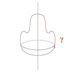
   Figure 2: An admissible rotation invariant surface $M$. In red, the geodesic $\gamma$ parametrized by $\theta\in[0,L]$.

4. $(M,g)$ a simply connected, compact Lie Group, with $H_{L}$ a bounded perturbation of $-\Delta_{g}$. This is the situation described in Section 4; further details will be discussed in Section 8.

5. $(M,g)=(\mathbb{R}^{2},g)$ with $g$ the Euclidean metric and $H_{L}$ a correction of $H_{An}$, cf. Eq. (5.1). This model will be discussed in detail in Section 8

Remark 5.5.

We point out that, in the examples 1,3 and 5, any $a$ in the joint spectrum $\Lambda$ has multiplicity 1 as a joint eigenvalue for $A_{1},\dots,A_{d}$, so we are in the situation of Remark 5.4.

On the contrary, in Examples 2 and 4 one deals with superintegrable quantum systems.

5.3 Semiclassical integrable systems

We end this section by recalling the definition of a semiclassical integrable system given by Colin de Verdière in his book [CDV]. First we recall that Colin de Verdière deals with semiclassical Hamiltonian operators on compact manifolds and studies the behavior of the various objects as $\hbar\to 0$.

Definition 5.6.

A semiclassical Hamiltonian $H$ on an $n$ dimensional manifold is said to be semiclassically completely integrable if there exist $n$ selfadjoint semiclassical operators $F_{1},...,F_{n}$ of order $0$ which are pairwise commuting s.t.

• The principal symbols $f_{1},...,f_{n}$ are in involution and almost everywhere independent;

• There exists a function $h_{L}\in C^{\infty}(\mathbb{R}^{n}:\mathbb{R})$ s.t.

  $$H=h_{L}(F_{1},...,F_{n})\ .$$

We remark that this definition does not make any reference to the action angle variables, but just to the existence of a sufficient number of “prime integrals” of the system.

In [CDV] one can also find a semiclassical analogue of Arnold Liouville theorem, showing that microlocally close to an invariant nondegenerate torus of the classical system, one can conjugate the Hamiltonian to a function of the operators $-i\hbar\partial_{j}$ (see also Charbonnel [Cha88]) on $\mathbb{T}^{d}$. We emphasize that the semiclassically integrable systems dealt with in such studies are more general than those covered by our definition, but on the contrary these semiclassical studies only give local results (see also [PVN14] for some semiglobal results). We remark that we do not know if the results of Sect. 6 can be extended to semiclassical integrable systems.

6 Perturbations of globally integrable quantum systems

In this section we will give the statement of two kind of results on perturbations of globally integrable quantum systems, the first one deals with linear perturbations, while the second deals with small nonlinear Hamiltonian perturbations.

The main assumption on the GIQS that we perturb is that $h_{L}$ is homogeneous and steep. The main tool used in the proof is a result of clustering of the joint spectrum $\Lambda$ that is given in the forthcoming Section 7 (see Theorem 7.4).

We recall that homogeneous functions are typically singular at the origin, but, in the context of pseudodifferential operators, the behavior of functions in a neighborhood of the origin is not important. In particular, in order to get rid of singularities at the origin remaining in the class of symbols, we give the following:

Definition 6.1.

A function $f\in C^{\infty}(\mathbb{R}^{d})$ is said to be homogeneous of degree $m$ at infinity if there exists $R>0$ such that

$$f(\lambda a)=\lambda^{m}f(a)\quad\forall\lambda>1\,,\quad\forall|a|\geq R\,.$$

We recall, from [GCB16], the definition of steepness:

Definition 6.2 (Steepness).

Let ${\mathcal{U}}\subset\mathbb{R}^{d}$ be a bounded connected open set with nonempty interior. A function $h_{0}\in C^{1}({\mathcal{U}})$, is said to be steep in ${\mathcal{U}}$ with steepness radius ${\tt r}$, steepness indices $\alpha_{1},\dots,\alpha_{d-1}$ and (strictly positive) steepness coefficients ${\tt B}_{1},...,{\tt B}_{d-1}$, if its gradient $w_{i}(a):=\frac{\partial h_{0}}{\partial a_{i}}(a)$ fulfills: $\displaystyle{\inf_{a\in{\mathcal{U}}}\|w(a)\|>0}$ and for any $a\in{\mathcal{U}}$ and for any $s$ dimensional linear subspace $M\subset\mathbb{R}^{d}$ orthogonal to $w(a)$, one has

$$\max_{0\leq\eta\leq\xi}\min_{u\in M:\|u\|=1}\|\Pi_{M}w(a+\eta u)\|\geq{\tt B}_{s}\xi^{\alpha_{s}}\quad\forall\xi\in(0,{\tt r}]\ ,$$ (6.1)

where $\Pi_{M}$ is the orthogonal projector on $M$; the quantities $u$ and $\eta$ are also subject to the limitation $a+\eta u\in{\mathcal{U}}$.

It is well known that steepness is generic. We also recall that all convex or quasiconvex functions are also steep.

A very useful sufficient condition for steepness is contained in the following theorem by Niederman [Nie06]. This is the theorem that we used in order to verify steepness in our concrete applications.

Theorem 6.3 (Niederman).

Let $h_{L}$ be a function real analytic in an open set ${\mathcal{U}}\subset\mathbb{R}^{d}$. Assume that $h_{L}$ has no critical points in ${\mathcal{U}}$, and its restriction $h\big{|}_{M}$ to any affine subspace $M\subset\mathbb{R}^{d}$ admits only isolated critical points, then $h_{L}$ is steep on any compact subset of ${\mathcal{U}}$.

So, we concentrate on perturbations of linear systems with Hamiltonian $H_{L}$ which is globally integrable quantum system, namely $H_{L}=h_{L}(A)$ and make the following assumption

Assumption (L).

$h_{L}$ is homogeneous of degree ${\tt d}>1$ at infinity and steep in an open set ${\mathcal{U}}\subset B_{1}\setminus B_{1/2}$ with the property that

$$\Lambda\cap{\mathcal{U}}=\Lambda\cap(B_{1}\setminus B_{1/2})\ .$$

6.1 Linear Perturbations: spectral stability and growth of Sobolev norms

6.1.1 Stability of the majority of eigenvalues

The first result we are going to present is a stability result of the majority of eigenvalues of $H_{L}$ when one adds a perturbation which is relatively bounded with respect to $H_{L}$ this is a generalization of Theorems 2.8 of [BLM20] and 2.8 of [BLR22].

First we consider the general case where the common eigenvalue possible have some multiplicity.

In this case it is possible to compute the first correction to the eigenvalues bifurcating from the majority of eigenvalues of $H_{L}$. This requires to define the average of the perturbation $V$, namely the operator

$$\langle V\rangle:=\frac{1}{(2\pi)^{d}}\int_{\mathbb{T}^{d}}e^{-{\rm i}\varphi\cdot A}Ve^{{\rm i}\varphi\cdot A}d\varphi\,,$$ (6.2)

which commutes with all the actions. Denote also

$$\Pi_{a}:=\Pi_{a^{1}}...\Pi_{a^{d}}$$ (6.3)

the projector on the common eigenspace of the actions corresponding to the common eigenvalue $a=(a^{1},...,a^{d})$, and denote by $n_{a}$ the dimension of $\Pi_{a}{\mathcal{H}}$, namely the multiplicity of the common eigenvalues, then the operator $\Pi_{a}\langle V\rangle\Pi_{a}$, gives the first variation of the eigenvalues bifurcating from $\lambda_{a}$. Precisely, denote by $\mu_{a,j}$ the eigenvalues of $\Pi_{a}\langle V\rangle\Pi_{a}$, then we have the following:

Theorem 6.4.

Consider the operator

$$H:=H_{L}+V\ ,$$ (6.4)

assume that $H_{L}$ fulfills assumption (L) and $V\in{\mathcal{A}}^{{\tt b}}$ with ${\tt b}<{\tt d}$. Then there exist a set $\Omega\subset\mathbb{R}^{d}$ and number $m_{2}<{\tt b}$ such that the following holds. $\Omega\cap\Lambda$ has density one at infinity, namely there exists $\rho>0$ such that

$$1-\frac{\sharp(\Omega\cap\Lambda\cap B_{R})}{\sharp(B_{R}\cap\Lambda)}={\mathcal{O}}(R^{-\rho})\,,$$ (6.5)

and $\forall a\in\Omega$ and any $j=1,...,n_{a}$ there exists an eigenvalue $\lambda_{a,j}$ of (6.4) fulfilling

$$|\lambda_{a,j}-\lambda_{a}-\mu_{a,j}|\lesssim\langle a\rangle^{m_{2}}\ .$$

In the case in which the common eigenvalues of the actions have no multiplicity one can give a more precise result, to this end we need first the following:

Definition 6.5.

Given a function $f:{\mathcal{V}}\subseteq\mathbb{R}^{d}\rightarrow\mathbb{R}$, we say that $f$ admits an asymptotic expansion,

$$f\sim\sum_{j}f_{j}\,,$$ (6.6)

if there exist a real sequence $\{m_{j}\}_{j\in\mathbb{N}}$ and a sequence $\{f_{j}\}_{j\in\mathbb{N}}$ of smooth functions $f_{j}:{\mathcal{V}}\rightarrow\mathbb{R}$ such that

$$m_{j+1}<m_{j}\quad\forall j\,,\quad m_{j}\rightarrow-\infty\quad\text{as}\quad j\rightarrow\infty\,,$$ (6.7)

$$|f_{j}(a)|\leq C_{j}\langle a\rangle^{m_{j}}\quad\forall a\,,$$ (6.8)

$$\left|f(a)-\sum_{j=0}^{N}f_{j}(a)\right|\leq C_{N}\langle a\rangle^{m_{N+1}}\quad\forall a,\quad\forall N\in\mathbb{N}\,.$$ (6.9)

Theorem 6.6.

Under the same assumptions of Theorem 6.4, assume also that the multiplicity of each common eigenvalues of the actions is 1 (as in Remark 5.4). Then there exist a sequence of smooth functions $z_{j}:{\mathcal{C}}\rightarrow\mathbb{R}$, with ${\mathcal{C}}$ as in Definition 5.2, such that the functions $z_{j}$ depend on $a$ only, and $\forall a\in\Omega\cap\Lambda$ there exists an eigenvalue $\lambda_{a}$ of (6.4) which admits the asymptotic expansion

$$\lambda_{a}\sim h_{L}(a)+\sum_{j\geq 0}z_{j}(a)\ .$$ (6.10)

Such a theorem ensures that in the case of multiplicity one, the majority of the eigenvalues of the perturbed problem are stable, namely they move only by asymptotically small quantities and furthermore admit an asymptotic expansion.

It is also possible to give a description of all the eigenvalues outside $\Omega$, following the presentation of [BLM22b], but the corresponding precise statement is quite complicated, so we avoid to give it here.

6.1.2 Time dependent perturbations

The second kind of results deals with the problem of growth of Sobolev norms, when the perturbation is time dependent. This is contained in the following Theorem.

Theorem 6.7.

[Main Theorem of [BL22]] Let $H=H(t)$ be of the form

$$H(t):=H_{L}+V(t)$$ (6.11)

with $H_{L}$ fulfilling assumption (L). Assume also that $V(\cdot)\in C^{\infty}_{b}\left(\mathbb{R};{\mathcal{A}}^{\tt b}\right)$ is a family of self-adjoint pseudodifferential operators with ${\tt b}<{\tt d}$; then for any $s\geq 0$ and for any initial datum $\psi\in{\mathcal{H}}^{s}$ there exists a unique global solution $\psi(t):={\mathcal{U}}(t,\tau)\psi\in{\mathcal{H}}^{s}$ of the initial value problem

$${\rm i}\partial_{t}\psi(t)=H(t)\psi(t)\,,\quad\psi(\tau)=\psi\,,$$ (6.12)

furthermore, for any $s>0$ and $\varepsilon>0$ there exists a positive constant $K_{s,\varepsilon}$ such that for any $\psi\in{\mathcal{H}}^{s}$

$$\|{\mathcal{U}}(t,\tau)\psi\|_{s}\leq K_{s,\varepsilon}\langle t-\tau\rangle^{\varepsilon}\|\psi\|_{s}\ ,\quad\forall t,\tau\in\mathbb{R}\,.$$ (6.13)

In particular Theorem 6.7 applies to the following equations:

1. Quantum particle on $\mathbb{T}^{n}$ subjected to electro-magnetic potential:

   $${\rm i}\partial_{t}\psi=\sum_{j=1}^{n}({\rm i}\partial_{j}+B_{j}(t,x))^{2}\psi+W(t,x)\psi\,,\quad x\in\mathbb{T}^{n}\,,$$ (6.14)

   with $B_{1},\dots,B_{n},W\in{\mathcal{C}}^{\infty}_{b}(\mathbb{R};\mathbb{T}^{n})$. This case was also studied in [BLM22a], with techniques specific to the torus.

2. Perturbed two-dimensional quantum anharmonic oscillator:

   $${\rm i}\partial_{t}\psi=-\frac{1}{2}\Delta\psi+\frac{1}{2\ell}\|x\|^{2\ell}\psi+{\rm i}\sum_{i,j=1,2}v_{ij}(t)x_{i}\partial_{x_{j}}\psi\,,\quad x\in\mathbb{R}^{2}$$ (6.15)

   with $v_{i,j}(t)\in{\mathcal{C}}^{\infty}_{b}(\mathbb{R})$.

3. Quantum particle on any one of the manifolds of Subsect. 5.2 with time dependent potential:

   $${\rm i}\partial_{t}\psi=-\Delta_{g}\psi+V(t)\psi\,,$$ (6.16)

   with $V\in{\mathcal{C}}^{\infty}_{b}(\mathbb{R};M)$.

Remark 6.8.

The classical counterpart to the problem of bounding the growth of Sobolev norms for (6.14) was treated in [Bam24] for a particle on the torus; there the following result was proven: consider the classical Hamiltonian

$$h(x,\xi)=\frac{1}{2}\sum_{j=1}^{n}(\xi_{j}-B_{j}(t,x))^{2}+W(t,x)\,,\quad(x,\xi)\in\mathbb{T}^{n}\times\mathbb{R}^{n}\,,$$ (6.17)

with $B_{1},\dots,B_{n},W\in{\mathcal{C}}^{\infty}_{b}(\mathbb{R}\times\mathbb{T}^{n})$. Then for any $\varepsilon>0$ there exists $C_{\varepsilon}>0$ such that all solutions of the Hamilton equations generated by $h$ satisfy

$$\|\xi(t)\|\leq C_{\varepsilon}\langle t\rangle^{\varepsilon}(1+\|\xi(0)\|)\ ,\quad\forall t\in\mathbb{R}\,.$$

6.2 Nonlinear Hamiltonian perturbations

Concerning nonlinear perturbations, we have to restrict to the case of operators on compact manifolds so we assume that $M$ is a compact manifold, and consider a nonlinear PDE of the form

$${\rm i}\psi_{t}=H_{L}\psi+P(\psi,\bar{\psi},x)\ ,$$ (6.18)

where $P$ is a Hamiltonian vector field whose properties will be specified in a while. Furthermore, besides assumption (L), we are going to make a nonresonance assumption on the eigenvalues of $H_{L}$; this is typically achieved by considering the case where $h_{L}$ depends on some external parameters that are used to tune the frequencies. This is the way we proceed in applications.

We start by giving the precise assumption on $P$.

Assumption (NL).

There exists a function $F\in C^{\infty}({\mathcal{V}}\times{\mathcal{V}}\times M;\mathbb{C})$ with ${\mathcal{V}}\subset\mathbb{C}$ a neighborhood of the origin with the following properties

• $P=\partial_{\bar{\psi}}F$,

• there exists $C$ s.t. for any $z\in{\mathcal{V}}$ one has $F(z,\bar{z},x)\in\mathbb{R}$, and

  $$|F(z,\bar{z},x)|\leq C|z|^{3}\ .$$

Actually a slightly more general assumption is enough and this is needed for the application to the nonlinear stability of the ground state in NLS, but we will not give here its abstract form.

We are now going to state the nonresonance assumption on the eigenvalues of $H_{L}$. As we will discuss in a while, this is a generalization of “0-th Melnikov condition”, whose standard form is

$$\begin{gathered}\omega_{a^{(1)}}\pm\omega_{a^{(2)}}\pm...\pm\omega_{a^{(r)}}\not=0\ \quad\Longrightarrow\\ \left|\omega_{a^{(1)}}\pm\omega_{a^{(2)}}\pm...\pm\omega_{a^{(r)}}\right|\geq\frac{\gamma_{r}}{(\max|a^{(j)}|)^{\tau_{r}}}\ .\end{gathered}$$ (6.19)

To give the precise statement denote by

$$\omega_{a}:=h_{L}(a)\ ,\ a\in\Lambda$$

the eigenvalues of $H_{L}$ and remark that by the assumption on the homogeneity of $h_{L}$ one has a bound on the cardinality of the set of eigenvalues in a ball. From such a bound it is easy to deduce the following clustering property

Lemma 6.9.

There exist two sequences $\alpha_{n}$, $\beta_{n}$ $n\in\mathbb{N},\ n\geq 0$ with $\alpha_{n}<\beta_{n}<\alpha_{n+1}$ and such that

• $h_{L}(\Lambda)\subset\bigcup_{n}[\alpha_{n},\beta_{n}]$;

• $\beta_{n}-\alpha_{n}\leq{2}$;

• $\alpha_{n+1}-\beta_{n}\geq 2n^{-d/{\tt d}}$.

The nonresonance condition that we are going to assume ensures that one can use Birkhoff normal form procedure in order to eliminate from the nonlinearity terms enforcing exchanges of energy among modes labeled by indexes belonging to different intervals. This requires to characterize the linear combination of frequencies which correspond to monomials enforcing such exchange of energy. So, we give the following definition

Definition 6.10.

Given $r\in\mathbb{N}$ and $j\in\left\{0,...r\right\}$, a set of indexes $(a^{(1)},...,a^{(r)})\in\Lambda^{r}$ will be said to be dangerous if $r$ is even and for any $l=1,...,r/2$ there exists an interval $[\alpha_{l},\beta_{l}]$ with the property that

$$a^{(l)}\ \text{and}\ a^{(l+r/2)}\in[\alpha_{l},\beta_{l}]\ ,\forall l=1,...,r/2\ .$$ (6.20)

A sequence which is not dangerous is called nondangerous.

Assumption (NR).

For any $r\geq 3$, there are constants $\gamma_{r},\tau_{r}>0$ such that $\forall j=1,...,r$ one has

$$\left|\sum_{l=1}^{j}\omega_{a^{(l)}}-\sum_{l=j+1}^{r}\omega_{a^{(l)}}\right|\geq\frac{\gamma_{r}}{\left(\max{|a^{(l)}|}\right)^{\tau_{r}}}\,.$$ (6.21)

for any non dangerous sequence $(a^{(1)},...,a^{(r)})$. For dangerous sequences we require (6.21) to hold only for $j\not=r/2$.

The following theorem is the main abstract result of [BFLM24].

Theorem 6.11.

Consider the Hamiltonian system (6.18). Assume Hypotheses (NL) and (NR), then for any integer $r\geq 3$, there exists $s_{r}\in\mathbb{N}$ such that, for any $s\geq s_{r}$, there are constants $\epsilon_{0}>0$, $c>0$ and $C$ for which the following holds: if the initial datum $\psi_{0}\in H^{s}(M,\mathbb{C})$ fulfills

$$\epsilon:=\left\|\psi_{0}\right\|_{s}<\epsilon_{0}\,,$$

then the Cauchy problem has a unique solution $u\in\mathcal{C}^{0}\left((-T_{\epsilon},T_{\epsilon}),H^{s}(M,\mathbb{C})\right)$ with $T_{\epsilon}>c\epsilon^{-r}$. Moreover, one has

$$\|\psi(t)\|_{s}\leq C\epsilon,\quad\forall t\in(-T_{\epsilon},T_{\epsilon})\ .$$ (6.22)

In particular, in [BFLM24] we show that Theorem 6.11 applies to the following models:

1. Schrödinger equation with convolution potential on one of the manifolds $M$ of the examples 1, 2, 3, 4, of Subsection 5.2

   $${\rm i}\partial_{t}\psi=-\Delta_{g}\psi+V\ast\psi+f(x,|\psi|^{2})\psi\,,\quad x\in M\,,$$ (6.23)

   with $f(x,\cdot)$ a smooth function having a zero of order at least $2$ at $0$, and $V$ belonging to a full measure subset of

   $${\mathcal{V}}_{m}:=\left\{V=\{V_{k}\}_{k\in\mathbb{Z}^{d}}\ \left|\ \langle k\rangle^{m}|V_{k}|\in\left[-\frac{1}{2},\frac{1}{2}\right]\right.\right\}\quad\text{for some }m>0\,.$$

   The case of $M=\mathbb{T}^{d}$ with a flat metric was already dealt with in [BFM24].

2. Beam equation on one of the manifolds $M$ of the examples 1, 2, 3, 4, of Subsection 5.2

   $$(\partial_{tt}+\Delta_{g}^{2}+m)u=-\partial_{u}F(x,u)\,,$$ (6.24)

   with $F\in{\mathcal{C}}^{\infty}(M\times{\mathcal{V}};\mathbb{R})$, where ${\mathcal{V}}$ is a neighborhood of the origin, having a zero of order at least 3 at $u=0$, and $m$ belonging to a full measure subset of $\mathbb{R}^{+}$.

3. Stability of the ground state in Nonlinear Schrödinger equation on one of the above manifolds

   $${\rm i}\partial_{t}\psi=-\Delta_{g}\psi+f(|\psi|^{2})\psi\,,$$ (6.25)

   with $f\in{\mathcal{C}}^{\infty}({\mathcal{V}};\mathbb{R})$ having a zero of order at least 1 at the origin. Then, for any $p_{0}\in{\mathcal{V}}\cap\mathbb{R}^{+}$ the plane wave

   $$\psi_{\star}(t)=\sqrt{p_{0}}e^{{\rm i}\nu t}\,,\quad\nu=f(p_{0})\,,$$ (6.26)

   is a solution of (6.25). In this case, from the abstract Theorem 6.11 we deduce the following:

   Theorem 6.12.

   Let $\bar{\lambda}$ be the minimum nonvanishing eigenvalue of $-\Delta_{g}$ and assume there exists $\bar{p}_{0}>0$ such that $\bar{\lambda}+2f(p_{0})>0$ for any $p_{0}\in(0,\bar{p}_{0}]$. Then there exists a zero measure set $\mathcal{P}\subset(0,\bar{p}_{0}]$ such that if $p_{0}\in(0,\bar{p}_{0}]\setminus\mathcal{P}$ then for any $r\in\mathbb{N}$ there exists $s_{r}$ for which the following holds. For any $s\geq s_{r}$, there exist constants $\epsilon_{0}$ and $C$ such that if the initial datum $\psi_{0}$ fulfills

   $$\|\psi_{0}\|_{0}^{2}=p_{0},\qquad\inf_{\alpha\in\mathbb{T}}\|\psi_{0}-\sqrt{p_{0}}e^{-i\alpha}\|_{s}=\epsilon\leq\epsilon_{0}\,,$$

   then the corresponding solution fulfills

   $$\inf_{\alpha\in\mathbb{T}}\|\psi(t)-\sqrt{p_{0}}e^{-i\alpha}\|_{s}\leq C\epsilon\qquad\forall\,|t|\leq C\epsilon^{-r}\ .$$

7 Nekhoroshev-Bourgain partition of the joint spectrum

In this section we give a partition of the joint spectrum $\Lambda$, which is the quantum analogue of the partition of the action space of a classical system in resonant blocks introduced by Nekhoroshev in order to prove his celebrated theorem on exponential stability of quasi integrable systems. It turns out that such a partition also has a remarkable property that was introduced by Bourgain in order to prove KAM type results for nonlinear wave and Schrödinger equation on $\mathbb{T}^{d}$.

As a result, this partition is the main tool for proving all the results of the previous section.

7.1 Classical Nekhoroshev Theorem and classical Nekhoroshev’s Partition

We start with recalling the classical Nekhoroshev Theorem:

Theorem 7.1.

Let $h:{\mathcal{A}}\times\mathbb{T}^{n}\rightarrow\mathbb{R}$ be a function of the form

$$h(a,\alpha)=h_{L}(a)+\varepsilon v(a,\alpha)\,,$$

where $h_{L}$ and $v$ are analytic on ${\mathcal{A}}$ and $h_{L}$ is steep on ${\mathcal{A}}$. Then there exist $\varepsilon_{0}>0$ $\mathtt{a},{\tt b}>0$ such that, defining ${\mathcal{U}}:=\{a\in{\mathcal{A}}\ |\ \operatorname{dist}(a,\partial{\mathcal{A}})\geq 2\varepsilon^{\mathtt{b}}\}$, if $|\varepsilon|<\varepsilon_{0}$, then for all initial data in ${\mathcal{U}}\times\mathbb{T}^{n}$ one has

$$\|a(t)-a(0)\|\leq\varepsilon^{\mathtt{b}}\quad\forall|t|\leq\varepsilon^{-1}e^{\varepsilon^{-{\mathtt{a}}}}\,.$$ (7.1)

The classical proof as formulated by Nekhoroshev in [Nek77, Nek79] (see also [GCB16, Gio03, BL20, Bam24]) is based on two steps: an analytic part, in which the Hamiltonian $h$ is put in local normal form, removing all non resonant contributions, and a geometric part, based on the analysis of resonances in the space of actions. We now are going to describe the latter geometric analysis of resonances and its role in the proof of Nekhoroshev Theorem, in order to enlighten the similarities with the procedure we adopt in the quantum case.

Actually, here we present the scheme of the proof of [BL20, Cai21], which is the closest to the quantum case and deals with long time stability in the case of smooth Hamiltonians:

Theorem 7.2 (${\mathcal{C}}^{\infty}$ Nekhoroshev Theorem).

Let $h:{\mathcal{A}}\times\mathbb{T}^{n}\rightarrow\mathbb{R}$ be of the form

$$h(a,\alpha)=h_{L}(a)+\varepsilon v(a,\alpha)\,,$$

with $h_{L}$ steep on ${\mathcal{A}}$ and $h_{L},v\in{\mathcal{C}}^{\infty}_{b}({\mathcal{A}}\times\mathbb{T}^{n};\mathbb{R})$. For any $b<\frac{1}{2}$ and $N>0$ there exist $\varepsilon_{N}>0$ and $C_{N}>0$ such that, for $0<\varepsilon<\varepsilon_{N}$, and any initial datum in ${\mathcal{U}}\times\mathbb{T}^{n}$, with ${\mathcal{U}}:=\{a\in{\mathcal{A}}\ |\ \operatorname{dist}(a,\partial{\mathcal{A}})\geq 2\varepsilon^{b}\}$, one has

$$\|a(t)-a(0)\|\leq\varepsilon^{b}\quad\forall|t|\leq C_{N}\varepsilon^{-N}\,.$$ (7.2)

The first step in the proof of Theorem 7.2 consists in performing a normal form procedure, which for any $N$ enables to conjugated the Hamiltonian $h$ to a new one of the form

$$h_{N}=h_{L}(a)+\varepsilon z_{N}(a,\alpha)+\varepsilon^{N}r_{N}(a,\alpha)\,,$$

with

$$z_{N}(a,\alpha)=\sum_{k\in\mathbb{Z}^{n}\atop\|k\|\leq K}\hat{z}_{k}(a)e^{{\rm i}k\cdot\alpha}\,,$$ (7.3)

$K=\varepsilon^{-\frac{1}{\zeta}}$ for some $\zeta>0$. Furthermore, there exists $\delta>0$ such that, for each $k$,

$$\operatorname{supp}\hat{z}_{k}(a)\subseteq\{a\ |\ |w(a)\cdot k|\leq\varepsilon^{\delta}\}\,,$$ (7.4)

where we recall that $w(\cdot):=\partial_{a}h_{L}(\cdot)$. Then the geometric part of the proof consists in analyzing the dynamics generated by $h_{L}+\varepsilon z_{N}$.

To this aim we first recall that a module of dimension $s=0,\dots,n$, is a subset $M\subseteq\mathbb{Z}^{n}$ such that $\operatorname{span}_{\mathbb{R}}(M)\cap\mathbb{Z}^{n}=M$. In this section we will denote by $M$ a submodulus of $\mathbb{Z}^{n}$.

Now we start by defining the resonant zones

$${\mathcal{Z}}^{(s)}_{M}:=\{a\ |\ \exists\ k_{1},\dots,k_{s}\quad\text{linearly indep. in }M\\ \text{s.t.}\quad|w(a)\cdot k_{j}|\leq\varepsilon^{\delta_{s}}\quad\forall j=1,\dots,s\}\,,$$ (7.5)

with a suitable sequences of increasing $\{\delta_{s}\}_{s=1}^{n}$ with $\delta_{1}=\delta$. For any $M$, the set ${\mathcal{Z}}^{(s)}_{M}$ collects all points $a$ such that $w(a)$ is resonant with some vectors in $M$. Its role is that, due to the form of the truncated Hamiltonian $h_{L}+\varepsilon z_{N}$ (see (7.3)–(7.4)), points in ${\mathcal{Z}}^{(s)}_{M}$ only move along directions parallel to $M$. Then, as long as the point $a(t)$ belongs to some resonant zone, its motion is easy to describe. A key step in the geometric part of the proof is then to understand how the resonant zones intersect one each other, and whether or not is possible to pass from one resonant zone from the other, visiting sooner or later all the action space (this is the well known phenomenon of overlapping of resonances).

(a) In yellow, cartoon of a resonant zone ${\mathcal{Z}}^{(s)}_{M}$, with $M=\operatorname{span}\{k\}$ for a given $k$. The dashed line corresponds to the curve $w(a)\cdot k=0$. Inside the zone, the motion generated by $h_{L}+\varepsilon z_{N}$ is parallel to $k$, pictured in turquoise.

(b) In yellow, two resonant zones associated to different modules. Their intersection is pictured in blue. In orange, a possible dangerous trajectory, passing from one zone to the other (overlapping of resonances, which we want to exclude).

In order to show that the latter phenomenon does not occur, one needs to define a more refined decomposition of the actions space ${\mathcal{A}}$ with respect to the one given by the resonant zones $\{{\mathcal{Z}}^{(s)}_{M}\}_{s,M}$. In particular, one proves the existence of a partition

$${\mathcal{A}}=\bigcup_{s=0}^{n}\bigcup_{\begin{subarray}{c}M\subseteq\mathbb{Z}^{n}\\ \operatorname{dim}M=s\\ M\text{module}\end{subarray}}\bigcup_{j\in\mathbb{N}}\mathcal{E}^{(s)}_{M,j}$$ (7.6)

in sets ${\mathcal{E}}^{(s)}_{M,j}$ such that

1. Each ${\mathcal{E}}^{(s)}_{M,j}$ has small diameter:

   $$\operatorname{diam}\left(\mathcal{E}^{(s)}_{M,j}\right)\leq\varepsilon^{\mathtt{c}_{2}}\quad\forall s,M,j\,.$$ (7.7)

2. Each ${\mathcal{E}}^{(s)}_{M,j}$ is contained in ${\mathcal{Z}}^{(s)}_{M}$, and is far away from having resonances with vectors not in $M$: in particular, if $k\in\mathbb{Z}^{n}$ satisfies

   $$|w(a)\cdot k|<\varepsilon^{\delta_{1}}\,,\quad\|k\|\leq K\,,$$ (7.8)

   then $k\in M$ and $a+\eta k\in{\mathcal{E}}^{(s)}_{M,j}$, provided $|\eta|\ll 1$.

3. ${\mathcal{E}}^{(s)}_{M,j}$ is invariant for the dynamics of $h_{L}+\varepsilon z_{N}$.

Note that, once this decomposition has been obtained, the statement of Theorem 7.2 essentially follows combining Items 1 and 3.

7.2 Invariant partition in the quantum case

Let us start with defining what we consider resonant in the case of a quasi-integrable quantum system:

Definition 7.3.

Let $\delta<{\tt d}-1$, $\mu>0$ and ${\tt R}>0$. We say $a\in\Lambda$ is resonant with $k\in\mathbb{Z}^{d}$ if

$$|w(a)\cdot k|<\|a\|^{\delta}\|k\|\,,\quad\|k\|\leq\|a\|^{\mu}\,,\quad\|a\|\geq\mathtt{R}\,,$$ (7.9)

where $w(a):=\partial_{a}h_{L}(a)$

A key point in proving Theorems 6.6, 6.4 and 6.7 is the following result, proven in [BL22] which gives the partition constituting the main step for the proof of the theorems of Sect. 6:

Theorem 7.4.

Under the assumptions of Theorem 6.7, there exist $0<\delta_{0}<{\tt d}-1$, $\mu_{0}>0$ and $\mathtt{R}_{0}>0$ such that, if $\delta_{0}<\delta<{\tt d}-1$, $0<\mu<\mu_{0}$, and $\mathtt{R}>\mathtt{R}_{0}$, the lattice $\Lambda$ admits a partition

$$\Lambda=\bigcup_{s=0}^{d}\bigcup_{\begin{subarray}{c}M\subseteq\mathbb{Z}^{d}\\ \operatorname{dim}M=s\\ M\text{module}\end{subarray}}\bigcup_{j\in\mathbb{N}}E^{(s)}_{M,j}$$ (7.10)

with the following properties:

• Each block $E^{(s)}_{M,j}$ is dyadic, in the sense that there exists $C>0$ such that

  $$\max\{\|a\|\ |\ a\in E^{(s)}_{M,j}\}\leq C\min\{\|a\|\ |\ a\in E^{(s)}_{M,j}\}$$ (7.11)

• If $a\in E^{(s)}_{M,j}$, there exists a vector $k\in\mathbb{Z}^{d}$ such that $a$ is resonant with $k$. Conversely, if $a$ is resonant with $k\in\mathbb{Z}^{d}$ in the sense of Definition 7.3, then $a+k\in E^{(s)}_{M,j}$.

• There exists $K>0$ such that, if $a\in E^{(s)}_{M,j}$ and $b\in E^{(s^{\prime})}_{M^{\prime},j^{\prime}}$ with $(s,M,j)\neq(s^{\prime},M^{\prime},j^{\prime})$, then

  $$\|a-b\|+|\omega_{a}-\omega_{b}|\geq K(\|a\|^{\mu}+\|b\|^{\mu})\,.$$ (7.12)

We start by remarking the analogies with the properties of the covering $\{{\mathcal{E}}^{(s)}_{M,j}\}$ exhibited in the classical case in Subsection 7.1: Item $(i)$ gives an upper bound on the diameter of the $E^{(s)}_{M,j}$, just as Property 1 of the sets ${\mathcal{E}}^{(s)}_{M,j}$. Furthermore, Item $(ii)$ states that, if $a$ is resonant with $k$, and $\|k\|$ is not too large, then $a+k$ belongs to the same block $E^{(s)}_{M,j}$, which is analogous to Property 2 of the sets ${\mathcal{E}}^{(s)}_{M,j}$.

We also remark that a first connection between Nekhoroshev’s partition and the spectral properties of the perturbations of the Laplacian was pointed out in [FFS15].

We now describe how Theorem 7.4 is used to prove the different theorems.

7.3 Linear perturbations

The first step of the proof consists in proving a “quantum normal form theorem” for Hamiltonians of the for (6.4) and (6.11).

This is contained in the following:

Proposition 7.5.

For any $N\in\mathbb{N}$ there exists a map $U_{N}\in{\mathcal{C}}^{\infty}_{b}(\mathbb{R};{\mathcal{B}}({\mathcal{H}}^{s},{\mathcal{H}}^{s}))$, such that $U_{N}(t)$ is unitary in ${\mathcal{H}}$ for any $t$ and $\psi$ solves (6.12) if and only if $\phi=U^{-1}_{N}(t)\psi$ solves

$${\rm i}\partial_{t}\phi=(H_{L}+Z_{N}(t)+R_{N}(t))\phi\,,$$ (7.13)

with $Z_{N}$ and $R_{N}$ self-adjoint operators as follows:

1. (Smoothing remainder) $R_{N}\in{\mathcal{C}}^{\infty}_{b}(\mathbb{R};{\mathcal{B}}({\mathcal{H}}^{s};{\mathcal{H}}^{s+N}))$ for any $s$

2. (Resonant normal form) $Z_{N}\in{\mathcal{C}}^{\infty}_{b}(\mathbb{R};{\mathcal{B}}({\mathcal{H}}^{s};{\mathcal{H}}^{s-{\tt b}}))$ for any $s$. Moreover, for any $a\in\Lambda$ let $\Pi_{a}$ be the projection operator defined in (6.3), then one has

   $$\Pi_{a}Z_{N}(t)\Pi_{a+k}\neq 0$$ (7.14)

   only if $a$ is resonant with $k$, or $a+k$ is resonant with $k$.

3. (Block diagonal structure) As a consequence, $Z_{N}$ is block diagonal along the blocks $E^{(s)}_{M,j}$ of Theorem 7.4, in the sense that for any $t$

   $$\Pi_{a}Z_{N}(t)\Pi_{b}\neq 0\quad\Rightarrow a,b\in E^{(s)}_{M,j}$$ (7.15)

   for some $s,M,j$.

Proposition 7.5 is based on an iterative procedure along which, for any $n$, at the $n-$th step one is able to eliminate from the perturbation $V_{n}(t)$ all terms

$$\Pi_{a}V_{n}(t)\Pi_{a+k}$$

such that both $a$ and $a+k$ are not resonant with $k$. Then all the remaining resonant contributions are collected in the normal form $Z_{N}$. This is the heart to the proof of Item 2. Note also that Item 3. follows directly combining Item 2. with property $(ii)$ of Theorem 7.4.

We now discuss how Proposition 7.5 enables to Prove Theorems 6.6, 6.4 and 6.7.

Sketch of the proof of Theorems 6.4 and 6.6.

We apply Proposition 7.5 in the time independent case. The main point is to define $\Omega$ as the set

$$\Omega:=\bigcup_{j}E^{(0)}_{j,M}$$

where $M=\left\{0\right\}$ is the trivial modulus. By Item $(ii)$ of Theorem 7.4, it follows that such a set contains all the points $a$ with the property that $w(a)$ is non- resonant, namely the only vector $k\in\mathbb{Z}^{d}$ such that (7.9) is satisfied is $k=0$. As a consequence, by Item 2 of Proposition 7.5 at these points the normal form $Z_{N}$ turns out to leave invariant the common eigenspaces of the actions, namely one has

$$Z_{N}\Pi_{a}=\Pi_{a}Z_{N}\Pi_{a}\ ,\quad\forall a\in\Omega\ .$$

Furthermore the algorithm of the proof of Proposition 7.5 also allows to show that $Z_{N}=\langle V\rangle+$lower order operators, with $\langle V\rangle$ defined by (6.2). This is why the spectrum of the restriction of $\langle V\rangle$ to $\Pi_{a}{\mathcal{H}}$ controls the first correction to the unperturbed eigenvalues. Then one should prove that the set $\Omega$ has density one at infinity. This can be obtained by following some ideas of the proof of the corresponding theorems of [BLM20] and [BLR22], but exploiting the steepness of $h_{L}$ instead than the arguments in [Rüs01].

The proof of Theorem 6.6 then simply follows by the remark that in this case the pseudo-differential operators commuting with all the actions are just functions of the actions. ∎

Sketch of the proof of Theorem 6.7.

By Item 3. of Proposition 7.5, neglecting the remainder $R_{N}(t)$, one can study the dynamics generated by $H_{L}+Z_{N}(t)$: by the fact that (1) $Z_{N}$ is diagonal with respect to the blocks, (2) $Z_{N}$ is self-adjoint so that the $L^{2}$ norm is conserved along the dynamics it generates, (3) since the blocks are dyadic, in each block the $L^{2}$ norm is equivalent to the ${\mathcal{H}}^{s}$ norm, one gets that, along the dynamics of $H_{L}+Z_{N}(t)$ one has

$$\|\varphi(t)\|_{{\mathcal{H}}^{s}}\lesssim_{s}\|\varphi(0)\|_{{\mathcal{H}}^{s}}\,.$$

Then the contribution of the smoothing remainder $R_{N}(t)$ is dealt with using Duhamel principle. Precisely, denote by ${\mathcal{U}}$ the flow map of the complete Hamiltonian (7.13) and by ${\mathcal{U}}_{app}$ the flow map of $H_{L}+Z_{N}(t)$, then, by Duhamel formula one has

$${\mathcal{U}}(t,\tau)\psi={\mathcal{U}}_{app}(t,\tau)\psi+\int_{\tau}^{t}{\mathcal{U}}_{app}(t,\tau^{\prime})(-{\rm i}R^{(N)}(\tau^{\prime})){\mathcal{U}}(\tau^{\prime},\tau)\psi\ d\tau^{\prime}\,,$$ (7.16)

Since $R^{(N)}\in C^{\infty}_{b}\left(\mathbb{R};{\mathcal{B}}({\mathcal{H}}^{0};{\mathcal{H}}^{N})\right)$ and since $H^{(N)}$ is self-adjoint in $L^{2}$, one gets

$$\|{\mathcal{U}}(t,\tau)\psi\|_{N}\lesssim\|\psi\|_{N}+\int_{\tau}^{t}\left\|R^{(N)}\right\|_{{\mathcal{B}}({\mathcal{H}}^{0};{\mathcal{H}}^{N})}\|{\mathcal{U}}_{app}(\tau^{\prime},\tau)\psi\|_{0}\ d\tau^{\prime}$$

$$\lesssim\|\psi\|_{N}+\int_{\tau}^{t}\left\|R^{(N)}\right\|_{{\mathcal{B}}({\mathcal{H}}^{0};{\mathcal{H}}^{N})}\|\psi\|_{0}\ d\tau^{\prime}\lesssim\|\psi\|_{N}+\langle t-\tau\rangle\|\psi\|_{0}\,,$$

$$\lesssim\langle t-\tau\rangle\|\psi\|_{N}\ .$$

Then using interpolation one immediately gets the thesis. ∎

7.4 Nonlinear perturbations

Sketch of the proof of Theorem 6.11.

Theorem 6.11 is the consequence of a Birkhoff normal form theorem conjugating (6.18) to its linear part plus a “normal form” plus a remainder which is of order $\epsilon^{N}$, with arbitrary $N$. Now, the main point is that, as it is well known, in order to perform such a normal form one has to consider small divisor corresponding to the terms one wants to eliminate from the Hamiltonian. The kind of normal form one can obtain is thus directly related to the kind of nonresonant conditions which is satisfied by the frequencies $\omega_{a}$. Using just the nonresonant condition (6.19) it is difficult to obtain a useful normal form in the general case. Actually the kind of nonresonant condition which is known to be very useful is

$$\begin{gathered}\omega_{a^{(1)}}\pm\omega_{a^{(2)}}\pm...\pm\omega_{a^{(r)}}\not=0\ \Longrightarrow\\ \left|\omega_{a^{(1)}}\pm\omega_{a^{(2)}}\pm...\pm\omega_{a^{(r)}}\right|\geq\frac{\gamma_{r}}{(\max_{3}|a^{(j)}|)^{\tau_{r}}}\,,\end{gathered}$$ (7.17)

where $\max_{3}$ is the third largest index among the $a^{(j)}$’s.

The idea here is that if one only tries to eliminate from the nonlinearities terms coupling different blocks $E_{M,j}$, then it turns out that for the corresponding small denominators one has a selection rule, which entails the fact that condition (6.19) implies condition (7.17) for all the small denominators that really matter.

The actual implementation of such a scheme is however quite complicated technically and we refer to [BFLM24] for more details (see also [BFM24]). ∎

8 Two examples of quantum integrable systems

In this section we analyze in detail two models and we show that they satisfy the assumptions of globally integrable quantum systems.

8.1 Anharmonic oscillator

Let us consider the operator

$$H_{An}=-\frac{\Delta}{2}+\frac{\left\|x\right\|^{2\ell}}{2\ell}\,,\quad x\in\mathbb{R}^{2}\,,$$ (8.1)

with $\ell\in\mathbb{N}$, $\ell>1$. In this case, the class ${\mathcal{A}}^{m}$ of pseudodifferential operators that we consider is the one defined in the second line of (5.3), and we are going to show that there exist a function $h_{L}$ and two action operators $A_{1},A_{2}\in{\mathcal{A}}^{1}$ such that

$$H_{An}=h_{L}(A_{1},A_{2})+R\,,$$

where $h_{L}$ coincides outside a neighborhood of the origin with the classical Hamiltonian written in action variables and $R$ is a lower order correction. It was proved in [BL22] that it is homogeneous of degree ${\tt d}=\frac{2\ell}{\ell+1}$; the operator $R$ is a lower order operator in ${\mathcal{A}}^{\tt b}$ with ${\tt b}<{\tt d}$. Remark that lower order terms are not relevant in order to satisfy the assumptions of Theorem 6.7, since the term $R$ can be included in the perturbation $V(t)$.

To prove this fact, following the strategy of Section 3: we start by remarking that $H_{L}$ is the quantization of the classical Hamiltonian

$$h_{An}(x,\xi)=\frac{\left\|\xi\right\|^{2}}{2}+\frac{\left\|x\right\|^{2\ell}}{2\ell}\,,$$ (8.2)

and start by constructing suitable action angle variables for it. The action variables that we choose for $h_{An}$ are the angular momentum

$$a_{2}(x,\xi):=x_{1}\xi_{2}-x_{2}\xi_{1}\$$ (8.3)

and the radial action $a_{r}$, namely the action of the effective Hamiltonian

$$h_{An}^{*}(r,p_{r},{\tt M}):=\frac{p_{r}^{2}}{2}+V_{{\tt M}}^{*}(r)\ ,\quad V_{{\tt M}}^{*}(r):=\frac{{\tt M}^{2}}{2r^{2}}+\frac{r^{2\ell}}{2\ell}\ ,$$ (8.4)

where $r={\|x\|}$, $p_{r}$ is the conjugated momentum and ${\tt M}$ is a particular value of the angular momentum, in the sense that we put ourselves on a level surface $\{(x,\xi)\ |\ a_{2}(x,\xi)={\tt M}\}$. In particular, one has

$$a_{r}=a_{r}(E,{\tt M}):=\frac{\sqrt{2}}{\pi}\int_{r_{m}}^{r_{M}}\sqrt{E-V^{*}_{\tt M}(r)}dr\ ,$$ (8.5)

where $0<r_{m}<r_{M}$ are the two solutions of the equation

$$E-V^{*}_{\tt M}(r)=0\ .$$

However, the actions $(a_{2},a_{r})$ are not good candidates to be quantized for our construction: indeed, while $a_{2}$ is a polynomial, $a_{r}$ turns out to have a singularity at ${\tt M}=0$. Anyway, this singularity can be removed, by performing a suitable unimodular transformation. This is the content of the following lemma, proved in [BLR22]:

Lemma 8.1.

[Lemma 4.5 of [BLR22]] The function

$$a_{1}(E,{\tt M}):=\left\{\begin{matrix}a_{r}(E,{\tt M})&for&{\tt M}>0\\ a_{r}(E,{\tt M})-{\tt M}&for&{\tt M}<0\end{matrix}\right.$$ (8.6)

has the following properties:

• it extends to a complex analytic function of ${\tt M}$ and $E$ in the region

  $$\left|{\tt M}\right|<\left(\frac{2\ell}{\ell+1}E\right)^{\frac{\ell+1}{2\ell}}\ ,\quad E>0\ .$$ (8.7)

• Define the cone ${\mathcal{C}}$ by

  $${\mathcal{C}}:=\left\{a\in\mathbb{R}^{2}\ ;\ a_{1}\geq 0\ \textrm{ if }a_{2}\geq 0\,,\quad a_{1}\geq|a_{2}|\ \textrm{ if }\ a_{2}<0\right\}\,.$$ (8.8)

  Then $h_{An}$ is an analytic function of $(a_{1},a_{2})$ in the interior of ${\mathcal{C}}$. Furthermore it is homogeneous of degree $\frac{2\ell}{\ell+1}$ as a function of $(a_{1},a_{2})$.

• Let $a=(a_{1},a_{2})$, there exist positive constants $C_{1},C_{2}$ s.t.

  $$C_{1}\langle a\rangle\leq{\tt k}_{0}\leq C_{2}\langle a\rangle\ .$$

Still, both $h_{An}$ and $a_{1}$ have a singularity at the origin. But, essentially due to the fact that the behavior of functions in a finite neighborhood of the origin does not play any fundamental role in symbolic calculus, this is easily fixed: we take $K\gg 1$ and we consider the decomposition

$$h_{An}(x,\xi)=h_{An}(x,\xi)\chi(Kh_{An}(x,\xi))+h_{An}(x,\xi)(1-\chi(Kh_{An}(x,\xi)))\,.$$ (8.9)

Now the first term is smoothing and, denoting

$$h_{L}(x,\xi):=h_{An}(x,\xi)(1-\chi(Kh_{An}(x,\xi)))\,,$$ (8.10)

actually $h_{L}$ is the expression of the function (8.10) in action variables $a^{\prime}_{1},a_{2}$, so that it coincides with $h_{An}$ (when written in terms of action variables) outside a neighborhood of the origin. Moreover, since by Item $(2)$ of Theorem 8.1 $h_{An}$ is a homogeneous function of $(a_{1},a_{2})$, $h_{L}$ is homogeneous at infinity.

Turning back to the quantum case, Theorem 3.1 and Theorem 3.2 of [CdV80] guarantee the following:

Theorem 8.2.

There exist two pseudodifferential operators $R_{j}\in{\mathcal{A}}^{\rho}$, with $\rho<1$, and two commuting pseudodifferential operators $A_{j}\in{\mathcal{A}}^{1}$ such that $A_{j}=Op^{W}(a_{j})+R_{j}$, and $A_{1},A_{2}$ are quantum actions according to Definition 5.2. In particular there exists a symbol $h\in S^{\frac{2\ell}{\ell+1}}_{AN}$ s.t.

$$H_{An}=h(A)\ .$$ (8.11)

Furthermore one has an asymptotic expansion

$$h=h_{L}+\text{lower order terms}.$$

with $h_{L}$ as in 8.10.

It remains to prove that $h_{L}$ satisfies Assumption L. This is done in the following steps: first one proves that there exists an open cone ${\mathcal{C}}_{e}$ containing $\overline{{\mathcal{C}}}\setminus\{0\}$ such that $h_{L}$ admits an homogeneous at infinity and analytic extension on ${\mathcal{C}}_{e}$. Then one checks that $h_{L}$ is steep on the cone ${\mathcal{C}}_{e}$; this is done in [BL22] by applying the criterion given in Theorem 6.3. This is verified following the methods of [BFS18], which consist in analyzing the expansion of the Hamiltonian at the circular orbits. In particular, we prove that the restriction of $h_{L}$ on any affine line only admits isolated critical points.

8.2 Lie Groups

Consider the Laplace Beltrami operator $-\Delta_{g}$ in $(M,g)$, where $M$ is a simply connected Lie group endowed with the bi-invariant metric $g$. Here the class of pseudo-differential operators ${\mathcal{A}}^{m}$ is given by the first line of 5.3, namely Hörmander class. The discussion in Section 4 shows that, if $A_{1},\dots,A_{d}$ are operators defined in (4.2) and $h_{L}:\mathbb{R}^{d}\rightarrow\mathbb{R}$ is the function defined by

$$h_{L}(a):=\sum_{i,j=1}^{d}a_{i}a_{j}{\tt f}_{i}\cdot{\tt f}_{j}\,,$$

with ${\tt f}_{1},\dots,{\tt f}_{d}$ the basis of fundamental weights of $M$ (see (4.1)), then one has

$$-\Delta_{g}=h_{L}(a)-F\,,\quad F:=\sum_{i,j=1}^{d}{\tt f}_{i}\cdot{\tt f}_{j}\,.$$ (8.12)

Now, as pointed out in Remark 4.1, the results of [Fis15] prove that $A_{1},\dots,A_{d}$ are pseudo-differential operators in ${\mathcal{A}}^{1}$. Moreover, since they act as Fourier multipliers on the basis of the fundamental weights $\{f_{j}\}_{j}$, they mutually commute and their joint spectrum is given by elements $\Lambda=\Lambda_{+}(M)$ in the cone of dominant weights of $M$. Since one also has

$$-\Delta_{g}\leq-\Delta_{g}+|F|\leq|h_{L}(A)|+2|F|\leq\sum_{j=1}^{d}A^{2}_{j}\|{\tt f}_{j}\|^{2}+2|F|\lesssim{\bf 1}+\sum_{j=1}^{d}A^{2}_{j}\,,$$

we deduce that ${\bf 1}+\sum_{j=1}^{d}A^{2}_{j}\lesssim-\Delta_{g}=K_{0}^{2}$. Hence we can conclude that $A_{1},\dots,A_{d}$ are a set of quantum actions according to Definition 5.2. We then have that $H_{L}=h_{L}(A)=-\Delta_{g}+F$ is globally integrable. Indeed, the function $h_{L}$ is homogeneous of degree two and convex, thus in particular it is steep and satisfies Assumption (L).

References

- [Bam03] D. Bambusi, Birkhoff normal form for some nonlinear PDEs, Comm. Math. Phys. 234 (2003), no. 2, 253–285. MR 1962462
- [Bam17] , Reducibility of 1-d Schrödinger equation with time quasiperiodic unbounded perturbations, II, Comm. Math. Phys. 353 (2017), no. 1, 353–378. MR 3638317
- [Bam18] , Reducibility of 1-d Schrödinger equation with time quasiperiodic unbounded perturbations, I, Trans. Amer. Math. Soc. 370 (2018), no. 3, 1823–1865.
- [Bam24] , A global Nekhoroshev theorem for particles on the torus with time dependent Hamiltonian, arXiv preprint: 2401.02822, 2024.
- [BD18] M. Berti and J.M. Delort, Almost Global Solutions of Capillary-gravity Water Waves Equations on the Circle, UMI Lecture Notes, Springer, 2018.
- [BDGS05] D. Bambusi, J.M. Delort, B. Grébert, and J. Szeftel, Almost global existence for Hamiltonian semilinear Klein‐Gordon equations with small Cauchy data on Zoll manifolds, Communications on Pure and Applied Mathematics 60 (2005).
- [Bea77] R. Beals, Characterization of pseudodifferential operators and applications, Duke Math. J. 44 (1977), no. 1, 45–57. MR 435933
- [Bel85] J. Bellissard, Stability and instability in quantum mechanics, Trends and developments in the eighties (Bielefeld, 1982/1983), World Sci. Publishing, Singapore, 1985, pp. 1–106. MR 853743
- [BFLM24] D. Bambusi, R. Feola, B. Langella, and F. Monzani, Almost global existence for some Hamiltonian PDEs on manifolds with globally integrable geodesic flow, arXiv preprint: 2402.00521, 2024.
- [BFM24] D. Bambusi, R. Feola, and R. Montalto, Almost global existence for some Hamiltonian PDEs with small Cauchy data on general tori, Communications in Mathematical Physics 405 (2024), no. 15, 253–285.
- [BFS18] D. Bambusi, A. Fusè, and M. Sansottera, Exponential stability in the perturbed central force problem, Regul. Chaotic Dyn. 23 (2018), no. 7-8, 821–841. MR 3910168
- [BG01] D. Bambusi and S. Graffi, Time quasi-periodic unbounded perturbations of Schrödinger operators and KAM methods, Comm. Math. Phys. 219 (2001), no. 2, 465–480. MR 1833810
- [BG03] D. Bambusi and B. Grébert, Forme normale pour NLS en dimension quelconque, C. R. Math. Acad. Sci. Paris 337 (2003), no. 6, 409–414. MR 2015085
- [BG06] D. Bambusi and B. Grébert, Birkhoff normal form for partial differential equations with tame modulus, Duke Mathematical Journal 135 (2006), no. 3, 507 – 567.
- [BGMR18] D. Bambusi, B. Grebert, A. Maspero, and D. Robert, Reducibility of the quantum Harmonic oscillator in -dimensions with polynomial time dependent perturbation, Analysis & PDEs 11 (2018), no. 3, 775–799.
- [BGMR21] D. Bambusi, B. Grébert, A. Maspero, and D. Robert, Growth of Sobolev norms for abstract linear Schrödinger equations, J. Eur. Math. Soc. (JEMS) 23 (2021), no. 2, 557–583. MR 4195741
- [BL20] D. Bambusi and B. Langella, A Nekhoroshev theorem, Mathematics in Engineering 3 (2020), no. 2, 117.
- [BL22] D. Bambusi and B. Langella, Growth of Sobolev norms in quasi integrable quantum systems, arXiv preprint: 2202.04505, 2022.
- [BLM20] D. Bambusi, B. Langella, and R. Montalto, On the spectrum of the Schrödinger operator on : a normal form approach, Communications in Partial Differential Equations 45 (2020), 1–18.
- [BLM22a] , Growth of Sobolev norms for unbounded perturbations of the Schrödinger equation on flat tori, J. Differential Equations 318 (2022), 344–358. MR 4387286
- [BLM22b] , Spectral asymptotics of all the eigenvalues of Schrödinger operators on flat tori, Nonlinear Analysis 216 (2022), 112679.
- [BLR22] D. Bambusi, B. Langella, and M. Rouveyrol, On the stable eigenvalues of perturbed anharmonic oscillators in dimension two, Communications in Mathematical Physics 390 (2022), no. 1, 309–348.
- [BM18] D. Bambusi and R. Montalto, Reducibility of 1-d Schrödinger equation with time quasiperiodic unbounded perturbations, III, J. Math. Phys. 59 (2018), no. 12, 122702.
- [BMM22] M. Berti, A. Maspero, and F. Murgante, Hamiltonian birkhoff normal form for gravity-capillary water waves with constant vorticity: almost global existence, arXiv preprint:2212.12255, 2022.
- [Cai21] S. Caimi, The Nekhoroshev theorem, Master Thesis, Universita’ degli Studi di Milano, 2021.
- [CDV] Y. Colin De Verdière, Méthodes semi-classiques et théorie spectrale, https://www-fourier.univ-grenoble-alpes.fr/ ycolver/All-Articles/93b.pdf.
- [CDV79] Y. Colin De Verdière, Sur le spectre des opérateurs elliptiques à bicaractéristiques toutes périodiques, Comment. Math. Helv. 54 (1979), no. 3, 508–522. MR 543346
- [CdV80] Y. Colin de Verdière, Spectre conjoint d’opérateurs pseudo-différentiels qui commutent. II. Le cas intégrable, Mathematische Zeitschrift 171 (1980), 51–74.
- [Cha88] A.-M. Charbonnel, Comportement semi-classique du spectre conjoint d’opérateurs pseudodifférentiels qui commutent, Asymptotic Anal. 1 (1988), no. 3, 227–261. MR 962310
- [Com88] M. Combescure, The quantum stability problem for some class of time-dependent Hamiltonians, Ann. Physics 185 (1988), no. 1, 86–110. MR 954669
- [DI17] J. Delort and R. Imekraz, Long-time existence for the semilinear Klein-Gordon equation on a compact boundary-less Riemannian manifold, Comm. Partial Differential Equations 42 (2017), no. 3, 388–416. MR 3620892
- [DLSV02] P. Duclos, O. Lev, P. Stovíček, and M. Vittot, Weakly regular Floquet Hamiltonians with pure point spectrum, Rev. Math. Phys. 14 (2002), no. 6, 531–568. MR 1915516
- [DS96] P. Duclos and P. Stovíček, Floquet Hamiltonians with pure point spectrum, Comm. Math. Phys. 177 (1996), no. 2, 327–347. MR 1384138
- [Fas05] F. Fassò, Superintegrable Hamiltonian systems: geometry and perturbations, Acta Appl. Math. 87 (2005), no. 1-3, 93–121. MR 2151125
- [FFS15] F. Fassò, D. Fontanari, and D. A. Sadovskií, An application of Nekhoroshev theory to the study of the perturbed hydrogen atom, Math. Phys. Anal. Geom. 18 (2015), no. 1, Art. 30, 23. MR 3430232
- [Fis15] V. Fischer, Intrinsic pseudo-differential calculi on any compact lie group, Journal of Functional Analysis 268 (2015), no. 11, 3404–3477.
- [GCB16] M. Guzzo, L. Chierchia, and G. Benettin, The steep Nekhoroshev’s theorem, Communications in Mathematical Physics 342 (2016), 569–601.
- [Gio03] A. Giorgilli, Notes on exponential stability of Hamiltonian systems, Pubblicazioni della Classe di Scienze, Scuola Normale Superiore, Pisa. Centro di Ricerca Matematica ”Ennio De Giorgi” (2003).
- [GIP09] B. Grébert, R. Imekraz, and E. Paturel, Normal forms for semilinear quantum harmonic oscillators, Comm. Math. Phys. 291 (2009), no. 3, 763–798. MR 2534791
- [Gor70] W. B. Gordon, On the relation between period and energy in periodic dynamical systems, J. Math. Mech. 19 (1969/70), 111–114. MR 245930
- [Hö85] L. Hörmander, The analysis of linear partial differential operators i-iii., Springer Berlin, 1985.
- [HR82] B. Helffer and D. Robert, Propriétés asymptotiques du spectre d’opérateurs pseudodifférentiels sur , Comm. Partial Differential Equations 7 (1982), no. 7, 795–882. MR 662451
- [Nek72] N. N. Nekhorošev, Action-angle variables, and their generalizations, Trudy Moskov. Mat. Obšč. 26 (1972), 181–198. MR 365629
- [Nek77] N. N. Nekhoroshev, Exponential estimate of the stability of near integrable Hamiltonian systems, Russ. Math. Surveys 32 (1977), no. 6, 1–65.
- [Nek79] , An exponential estimate of the time of stability of nearly integrable Hamiltonian systems. II, Trudy Sem. Petrovsk. (1979), no. 5, 5–50. MR 549621
- [Nek05] , Types of integrability on a submanifold and generalizations of Gordon’s theorem, Tr. Mosk. Mat. Obs. 66 (2005), 184–262. MR 2193433
- [Nie06] L. Niederman, Hamiltonian stability and subanalytic geometry, Ann. Inst. Fourier (Grenoble) 56 (2006), no. 3, 795–813. MR 2244230
- [Pro07] C. Procesi, Lie groups, Universitext, Springer, New York, 2007, An approach through invariants and representations. MR 2265844
- [PVN14] A. Pelayo and S. Vũ Ngoc, Semiclassical inverse spectral theory for singularities of focus–focus type, Commun. Math. Phys. 329 (2014), no. 2, 809–820 (en).
- [Rüs01] H. Rüssmann, Invariant tori in non-degenerate nearly integrable Hamiltonian systems, Regul. Chaotic Dyn. 6 (2001), no. 2, 119–204. MR 1843664