Can the splashback radius be an observable boundary of galaxy clusters?

The splashback radius was proposed as a physically motivated boundary of clusters as it sets the limit between the infalling and the orbitally dominated regions. However, galaxy clusters are complex objects connected to filaments of the cosmic web from which they accrete matter that disturbs them and modifies their morphology. In this context, estimating the splashback radius and the cluster boundary becomes challenging. In this work, we use a constrained hydrodynamical simulation of the Virgo cluster’s replica embedded in its large-scale structure to investigate the impact of its local environment on the splashback radius estimate. We identify the splashback radius from 3D radial profiles of dark matter density, baryons density, and pressure in three regions representative of different dynamical states: accretion from spherical collapse, filaments, and matter outflow. We also identify the splashback radius from 2D-projected radial profiles of observation-like quantities: mass surface density, emission measure, and Compton-$y$. We show that the splashback radius mainly depends on the dynamics in each region and the physical processes traced by the different probes. We find multiple values for the splashback radius ranging from 3.3$\pm$0.2 to 5.5$\pm$0.3 Mpc. Particularly, in the regions of collapsing and outflowing material, the splashback radii estimated from baryon density and pressure radial profiles overestimate that of the dark matter density profiles, which is considered the reference value originally defined from dark matter simulations. Consequently, caution is required when using the splashback radius as a boundary of clusters, particularly in the case of highly disturbed clusters like Virgo. We also discuss the detection of the splashback radius from pressure radial profiles, which could be more related to an accretion shock, and its detection from stacked radial profiles.

1 Introduction

Clusters of galaxies are tracers of the cosmic matter density and distribution as they are the most massive gravitationally bound structures in the Universe. They are thus used to put constraints on cosmological parameters via their number count (e.g., Planck Collaboration, 2014b; Salvati et al., 2018; Aymerich et al., 2024) or the baryon fraction (e.g., Wicker et al., 2023), which requires a precise and unbiased mass estimation and calibration (e.g., Salvati et al. 2019, Gianfagna et al. 2021, Lebeau et al. 2024, Aymerich et al. 2024 and references therein). This, in turn, necessitates the definition of a cluster boundary in which the mass is estimated. Assuming that galaxy clusters formed via the spherical collapse of initial overdensities (Gunn & Gott III, 1972), we can estimate their mass in a sphere of a characteristic radius. Considering the self-similar evolution of clusters (Kaiser, 1986), characteristic radii are also useful for comparing clusters through normalised quantities. In the past decade, a new physically-motivated radius setting the transition from free-fall to orbital motion of Dark Matter (DM) particles in N-body simulations has been proposed (Diemer & Kravtsov, 2014; Adhikari et al., 2014; More et al., 2015): the splashback radius, $R_{\text{sp}}$. It has been studied in various N-body and hydrodynamical cosmological simulations using dark matter, baryons and galaxies densities (e.g.,Diemer & Kravtsov 2014; Diemer et al. 2017; Mansfield et al. 2017; O’Neil et al. 2021; Aung et al. 2021; Towler et al. 2023) or galaxy radial velocities (Diemer & Kravtsov, 2014; Pizzardo et al., 2023). Diemer (2020) showed that using the splashback radius to define the halo mass provides mass functions more universal, that is, independent of redshift and cosmology as expected by theoretical models (e.g., Press & Schechter, 1974), than mass functions based on the virial mass or spherical overdensities masses. According to them, this confirms that $R_{\text{sp}}$ is a physically-motivated definition of a DM halo boundary.

However, $R_{\text{sp}}$, and thus $M_{\text{sp}}$ the mass enclosed in a sphere of this radius, was determined by following DM particles trajectories in Diemer (2020) (see Mansfield et al. 2017 for details). In contrast, in observations, we can only try to derive $R_{\text{sp}}$ from radial profiles or the radial velocities of galaxies. Given that galaxy clusters are connected to filaments of the cosmic web (e.g., Cautun et al., 2014; Peebles, 2020; Gouin et al., 2021, 2022, 2023; Galárraga-Espinosa et al., 2020, 2021, 2022), defining their boundary in this complex environment could be biased. Moreover, $R_{\text{sp}}$ is located in clusters’ outskirts, which can be very challenging to observe due to the signal’s faintness. Still, numerous tentative detections in various wavelengths were performed by stacking the observed signal of a sample of clusters to reach a sufficiently high signal-to-noise ratio. In the optical, both galaxy number density (e.g., More et al., 2016; Chang et al., 2018; Shin et al., 2019; Adhikari et al., 2021; Bianconi et al., 2021; Baxter et al., 2021; Rana et al., 2023) and weak lensing (Contigiani et al., 2019; Shin et al., 2021; Fong et al., 2022; Giocoli et al., 2024) were used. In the sub-millimetre wavelengths, through the thermal Sunyaev-Zel’dovich (tSZ, Sunyaev & Zeldovich, 1972) effect, a pressure decrease in the Intra Cluster Medium (ICM) was detected and associated with the splashback radius (e.g., Anbajagane et al., 2022, 2023; Rana et al., 2023).

In the present study, we investigate the sensitivity of $R_{\text{sp}}$ to the dynamics in cluster outskirts and its observability. To this end, we conduct a detailed study of a state-of-the-art constrained hydrodynamical simulation reproducing the Virgo cluster in its local environment (Sorce et al., 2021). We first present the methodology in Sect. 2, including selecting regions of accreting, outflowing and filament material to investigate the sensitivity of the splashback radius estimate to specific dynamics. We identify $R_{\text{sp}}$ either on DM or baryons density 3D radial profiles as well as on pressure 3D radial profiles in Sec. 3. Since we use a constrained replica of the Virgo cluster in its local environment (see Sorce et al. 2019 for the constraining method), we can produce projected maps along the-Milky-Way-to-Virgo line of sight in our simulation, which is consistent with Virgo’s observations. We thus identify $R_{\text{sp}}$ on 2D-projected radial profiles extracted from maps of mass surface density, X-rays emission measure, and Compton-$y$ signal in Sec. 4. Finally, we discuss our results in Sec. 5 before concluding in Sec. 6.

2 Methodology

In this section, we first introduce the Virgo simulated replica, define characteristic radii of galaxy clusters, present the method adopted to compute 3D and 2D-projected radial profiles, and finally identify the regions our study focuses on.

2.1 The Virgo replica simulation

Recently, Sorce et al. (2019) produced replicas of Virgo within its cosmic environment by using constrained initial conditions of the Local Universe (see Sorce et al. 2016 for details). This set of DM simulations is in remarkable agreement with observations. The most representative simulated halo was then re-used to produce a high-resolution hydrodynamical simulation of Virgo (Sorce et al., 2021), which also agrees well with observations. More details about the simulation and its agreement with observations can be found in Sorce et al. (2021) and Lebeau et al. (2024).

As all the CLONE (Constrained LOcal and Nesting Environment) simulations so far, the Virgo replica zoom-in simulation relies on the Planck Collaboration (2014a) cosmological parameters, namely total matter density $\Omega_{m}=0.307$, dark energy density $\Omega_{\Lambda}=0.693$, baryonic density $\Omega_{b}=0.048$, amplitude of the matter power spectrum at 8 Mpc/h $\sigma_{8}=0.829$, Hubble constant $H_{0}=67.77\leavevmode\nobreak\ \mathrm{km/s/Mpc}$ and spectral index $n_{s}=0.961$. This particular CLONE was produced using the RAMSES (Teyssier, 2002) Adaptive Mesh Refinement (AMR) code. The zoom region is contained in a 500 Mpc/h local Universe box, it is a 30 Mpc diameter sphere with a resolution of $8192^{3}$ effective DM particles of mass $m_{\mathrm{DM}}=3.10^{7}\leavevmode\nobreak\ \mathrm{M_{\odot}}$. The AMR grid has a finest cell size of 0.35 kpc. The simulation also contains sub-grid models for star formation, radiative gas cooling and heating, and kinetic feedback from the active galactic nucleus (AGN) and type II supernova (SN) similar to the Horizon-AGN implementation of Dubois et al. (2014, 2016). Furthermore, the AGN feedback model has been enhanced by orientating the jet according to the Black Hole (BH) spin (see Dubois et al. 2021 for details).

The properties of DM and baryons were extracted using the rdramses code first used in Renaud et al. (2013). The Tweed et al. (2009) halo finder has been used to identify the Virgo DM halo and its galaxies using the stars. We define the baryons as the gas in the simulation cells, in which hydrodynamics equations are solved following an Eulerian approach. In a first approach, we do not apply any density or temperature selection; baryons thus include the cold gas from galaxies. All the baryon cells and DM particles were used to compute the radial density profiles. On the contrary, to compute 3D pressure radial profile and produce Compton-$y$ maps, we selected cells of ionised gas, namely cells with a temperature above $10^{5}$K, which is the ionisation threshold, and removed the cells associated with the galaxies (see Lebeau et al. 2024 for more details). To produce projected emission measure maps from the ICM gas, we only selected the cells with a temperature above $10^{7}$K, given it is approximately the minimum observable temperature of X-ray telescopes.

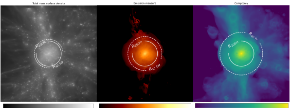
Figure 1: Projected maps of surface density (SD, left), emission measure (EM, centre) and Compton-$y$ ($y$, right). The projection follows the direction between the Milky Way’s assumed position and the Virgo cluster’s centre. The maps are 22.122 Mpc wide and contain $15728^{2}$ pixels. The circles represent $R_{\text{200m}}$ (solid-white), and $R_{\text{sp}}$ (dashed-white) identified on each 2D-projected profiles extracted from the maps.

2.2 Characteristic radii of galaxy clusters

Assuming a spherical collapse model (Gunn & Gott III, 1972), we estimate the mass of a galaxy cluster within a sphere of a given radius defining its boundary. A first physically-motivated boundary can be estimated using the virial theorem (Gunn & Gott III, 1972; Lacey & Cole, 1993; Peebles, 2020). A cluster at dynamic equilibrium considered as virialised has its potential energy ($E_{\mathrm{p}}$) equal to the opposite of twice its kinetic energy ($E_{\mathrm{k}}$), $E_{\mathrm{p}}+2E_{\mathrm{k}}=0$. The distance at which this equation is valid is the virial radius ($R_{\text{vir}}$) and defines a boundary inside which the galaxy cluster matter is at dynamical equilibrium. Following this theorem, we can estimate cluster masses with galaxy velocities in optical galaxy surveys (e.g., de Vaucouleurs 1960 for the Virgo cluster) or in numerical simulations (see Vogelsberger et al. 2020 for a review). For this Virgo replica simulation, we found $R_{\text{vir}}=2.1$ Mpc using the Tweed et al. (2009) halo finder .

However, $R_{\text{vir}}$ is not directly accessible when observing the ICM through the tSZ effect or in the X-rays since these observables trace the clusters’ thermodynamic properties. Consequently, we usually estimate cluster masses using scaling relations (Pratt et al., 2019, and references therein) or the hydrostatic equilibrium (e.g., Ettori et al., 2013) within radii enclosing a given overdensity. More precisely, we define a radius, $R_{\Delta\text{c}}$, at which the density is $\Delta$ times the critical density of the Universe

$$R_{\Delta\text{c}}=R(\rho=\Delta\rho_{\text{c}})\quad\mathrm{with}\quad\rho_{c}=3H^{2}/8\pi G.$$ (1)

The mass enclosed in a sphere of this radius is thus

$$M_{\Delta\text{c}}=\Delta\rho_{\text{c}}\frac{4}{3}\pi R_{\Delta_{c}}^{3}$$ (2)

The most widely used characteristic radii are $R_{\text{500c}}$ and $R_{\text{200c}}$. For our Virgo replica, $R_{\text{500c}}=1.1$ Mpc and $R_{\text{200c}}=1.7\leavevmode\nobreak\$Mpc.

Instead of using the critical density of the Universe, we can also use the mean matter density, $\rho_{\text{m}}=\rho_{\text{c}}\Omega_{\text{m}}$, and define $R_{\Delta\text{m}}$. Usually, we use $R_{\text{200m}}$ because it has been shown (e.g., Kravtsov & Borgani, 2012) that the ratio of the density at $R_{\text{vir}}$, $\rho_{\text{vir}}$, over $\rho_{\text{m}}$ is $\sim$200 ($\sim$178 in an Einstein-de Sitter Universe, see Bryan & Norman 1998 for other cosmologies). To compare with other works, we normalise every radial profile by $R_{\text{200m}}$. For our Virgo replica, $R_{\text{200m}}=2.9$ Mpc. The values of these characteristic radii are summarised in Tab.1 for comparison with the $R_{\text{sp}}$ identified in this work.

The focus of this study is the splashback radius, $R_{\text{sp}}$, introduced by works on N-body simulations (Adhikari et al., 2014; Diemer & Kravtsov, 2014; More et al., 2015). It was initially defined as the apocentre of the first orbit of DM particles free-falling onto a massive DM halo. It is a dynamic definition of a galaxy cluster since it sets the boundary between the region of infalling motion on the cluster and the region in which orbital motion dominates. Infalling particles will pile up at this radius as they inverse their radial velocity, so the particle density will strongly decrease beyond this characteristic radius. It can thus be identified as the steepest slope in the radial density profile. In other words, it is the minimum of the gradient of the radial density profile:

$$R_{\text{sp}}=R\left[\text{Min}\left(\frac{\text{dlog}(\rho)}{\text{dlog}(r)}\right)\right].$$ (3)

with Min for the minimum and $\rho$ the density of either DM, baryons or their sum.

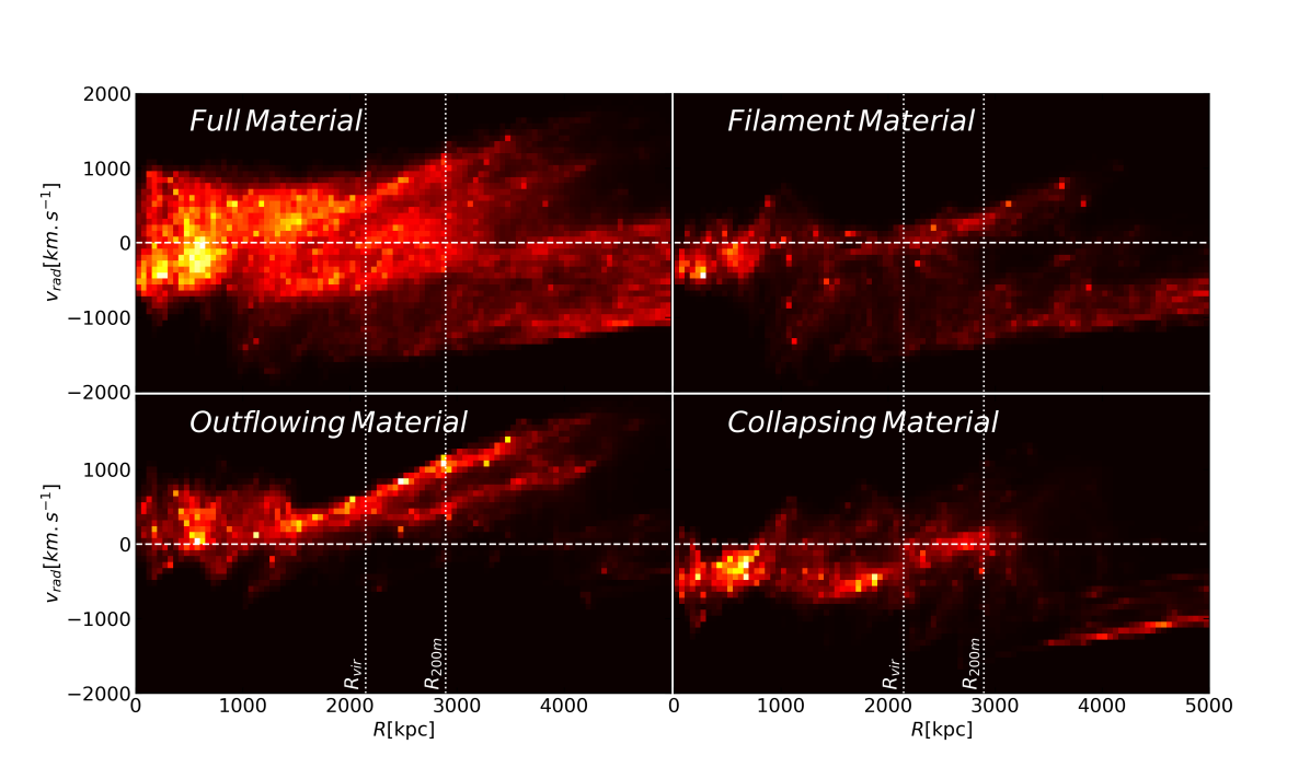
Figure 2: Radial distance-radial velocity phase-space diagram of the ionised gas using the Full Material in the zoom-in box (top-left), the region of Filament Material (top-right), the region of Outflowing Material (bottom-left) and the region of Collapsing Material (bottom-right).

2.3 3D and 2D-projected radial profiles

In this work, we will identify $R_{\text{sp}}$ as the radius of minimum gradient on radial profiles of DM, baryons, their sum but also pressure as other works (e.g., Shi, 2016; Towler et al., 2023) relate it to $R_{\text{sp}}$. We will also produce projected maps of observation-like quantities from which we will extract 2D-projected radial profiles and once again identify $R_{\text{sp}}$ as the radius of minimum gradient similar to Towler et al. (2023).

We adapt the procedure presented in Lebeau et al. (2024) to compute the radial profiles used for our analysis. We define a binning of 0.025 in log scale ranging from 200 kpc to the limit of the zoom-in region ($\sim$14.75 Mpc) minus the size of the biggest ($\sim$350 kpc) cells out of the zoom-in region. It avoids contamination from low-resolution cells at the borders of the zoom-in region, leading to an unphysical profile shape. For 3D density profiles (DM, baryons and their sum on Figs. 4 and 5), we sum the masses in each spherical shell and divide it by its volume. For 3D baryon properties (pressure, temperature, electron density and entropy in Fig. 6 in this work), we compute their mass-weighted mean. The error bars are given by the mass-weighted standard deviation and thus show the dispersion around the mean value.

We also compute observation-like quantities from which we derive 2D-projected profiles and try to identify $R_{\text{sp}}$. We build maps of surface density (SD) akin to lensing signal, emission measure (EM) in X-rays and integrated Compton-$y$ ($y$). The projected maps are built using the method detailed in Lebeau et al. (2024). They contain $15728^{2}$ pixels of 1.4065 kpc length and are 22.122 Mpc wide. We sum the contribution of all the cells along the line of sight in each pixel. In equations 4,5 and 6, $m_{\text{cell,i}}$, $l_{\text{cell,i}}$, $P_{\text{e,cell,i}}$, $n_{\text{e,cell,i}}$ and $n_{\text{p,cell,i}}$ are the mass, length, electron pressure, electron density and proton density of the $i$-th baryon cell and $m_{\text{part,j}}$ is the mass of the $j$-th DM particle.

We build the SD map by summing the DM particles and baryon cell masses in each pixel. For the baryon cells contributing to more than one pixel, the mass attributed to each pixel is the cell’s total mass divided by the number of occupied pixels. We then divide each pixel by its size; the map is in $\mathrm{M_{\odot}/kpc^{2}}$. The method is summarised in the following equation giving the SD in a pixel $\Sigma_{\text{px}}$

$$\Sigma_{\text{px}}=\left(\sum_{i}^{N_{\text{baryon\,cell\,in\,px}}}\frac{m_{\text{cell,i}}}{S_{\text{cell,i}}/S_{\text{px}}}+\sum_{j}^{N_{\text{DM\,particle\,in\,px}}}m_{\text{part,j}}\right)/S_{\text{px}}$$ (4)

where $S_{\text{px}}$ is the pixel surface and $S_{\text{cell,i}}$ is the surface of the $i$-th cell.

The pressure in the ICM of galaxy clusters can be studied via the tSZ effect (see Birkinshaw 1999 for a review) since it is proportional to the electron pressure integrated along the line of sight. To build the $y$ map, we sum the pressure in cells multiplied by their length in each pixel. The $y$ intensity in a pixel $y_{\text{px}}$ is

$$y_{\text{px}}=\frac{\sigma_{T}k_{\text{b}}}{m_{\text{e}}c^{2}}\sum_{i}^{N_{\text{baryon\,cell\,in\,px}}}P_{\text{e,cell,i}}\;l_{\text{cell,i}}$$ (5)

with $\sigma_{T}$ the Thomson cross section, $k_{B}$ the Boltzmann constant, $m_{e}$ the electron mass and $c$ the speed of light, $y$ is unitless.

Finally, the density in the ICM is investigated through X-rays observations (Sarazin, 1986). In the X-ray soft band, the EM is the proton density times the electron density integrated along the line of sight. To build the map from the simulation box, we sum the product of the proton density and the electron density in the cells with a temperature higher than $10^{7}\text{K}$ multiplied by their length in each pixel. The emission measure in a pixel, $EM_{\text{px}}$, is

$$EM_{\text{px}}=\sum_{i}^{N_{\text{baryon\,cell\,in\,px}}}n_{\text{p,cell,i}}n_{\text{e,cell,i}}\;l_{\text{cell,i}}$$ (6)

Following Eckert et al. (2012), it is expressed in $\mathrm{cm^{-6}Mpc}$.

In Fig. 1, we present the maps of SD (left), EM (centre) and $y$ (right). The colorbar is in the log scale below each map. The white solid circle is $R_{\text{200m}}$; the white dashed circle is $R_{\text{sp}}$ identified on the 2D-projected radial profile extracted from the map (see Fig. 7 in Sec. 4). All the maps show the filamentary structure connected to Virgo, on the SD map we observe the DM halos distribution, whereas on the EM and $y$ maps we see the diffuse gas, more particularly tracers of its density and pressure, respectively. We also see an almost empty area on the left part of the $y$ map.

We then extract 2D radial profiles (see Fig. 7) from the maps by computing the mean (similarly to pressure profiles, we discuss about using the median instead in Sec. 5) among the pixels in annuli using the same binning as for the 3D radial profiles. The error bars are the standard deviation over the pixels in the circular annuli. We choose a projection following the direction between the centre of the large-scale simulation box, almost centred on the Milky Way, and the centre of Virgo; it is thus comparable to a real Virgo observation. For every radial profile presented in this paper (Figs.4,5,6 and 7), both axes are in log scale and the radius in the abscissa is normalised by $R_{\text{200m}}$ (shown as a grey dashed vertical line) to compare with other studies.

2.4 Selection of studied regions in Virgo

Clusters originally accreted matter via spherical collapse before relaxing and virialising. Nowadays, they can still accrete matter from spherical collapse but also from cosmic filaments connected to them. These accretion regimes can take place at the same time in different regions of a single cluster. Hence, this work takes advantage of the zoom-in Virgo simulation embedded in its local environment to study the impact of the local environment, and so the dynamical state, on the estimation of the splashback radius in different regions. Using the radial distance-radial velocity phase-space diagram of the ionised gas, defined as baryon cells not belonging to galaxies and with $T>10^{5}$K, presented in Fig. 2, we select three regions that are representative of distinct accretion regimes: accretion due to spherical collapse, accretion from filament, and matter outflow. They have the same volume and radial range, enabling direct one-to-one comparisons between regions.

In Fig. 2, the radial velocity axis is in the range [-2000,2000] $\mathrm{km.s^{-1}}$ divided into 50 bins, the radial distance is in the range [0,5] Mpc divided into 100 bins. All the ionised gas in the zoom-in region, i.e. Virgo and its neighbourhood, is shown on the top-left panel. Throughout this paper, we refer to the full zoom-in region as Full Material. A 3D visualisation of the pressure in the zoom-in box is presented Fig. 3. The top panel shows the full box, and the bottom panel shows a slice in the cluster’s core along the simulation’s z-axis. The pressure is in $\mathrm{keV.cm^{-3}}$, it is shown in log scale in the range [-8,0].

On the top-right panel of Fig. 2, we observe that the majority of the ionised gas, in the range [1,5] Mpc, has a high negative radial velocity, indicating that it is falling onto the cluster without being slowed down while entering the ICM. It is a strong hint of the presence of a filament as shown in other works (e.g., Gouin et al., 2022; Vurm et al., 2023). In the following, we will call the matter, that is, baryons and DM, in this region Filament Material. It corresponds to the red box in Fig. 3 in which we see a large filament connected to Virgo that was already highlighted in Lebeau et al. (2024). On the contrary, we observe on the bottom-left panel of Fig. 2 that most of the ionised gas, in the range [1.5,4] Mpc, has a positive radial velocity, indicating that it is moving away from the cluster. There is no accretion in this region as there is almost no ionised gas with a negative radial velocity outside the cluster; we will thus call the matter in this region Outflowing Material. It corresponds to the green box in Fig. 3 in which we observe a minimal amount of pressure, and so matter, outside the cluster and an almost spherical cluster shape. Finally, on the bottom-right panel of Fig. 2, we observe that the ionised gas is falling on the cluster but with a much lower absolute radial velocity than for the Filament Material, particularly in the range [1,2] Mpc, it shows that it has been slowed down while entering the ICM. We will consider that we are in the case of a spherical collapse; we will thus call the matter in this region Collapsing Material. It corresponds to the blue box in Fig. 3, Virgo is also quite spherical in this region, but there is more infalling matter outside the cluster compared to the region of Outflowing Material.

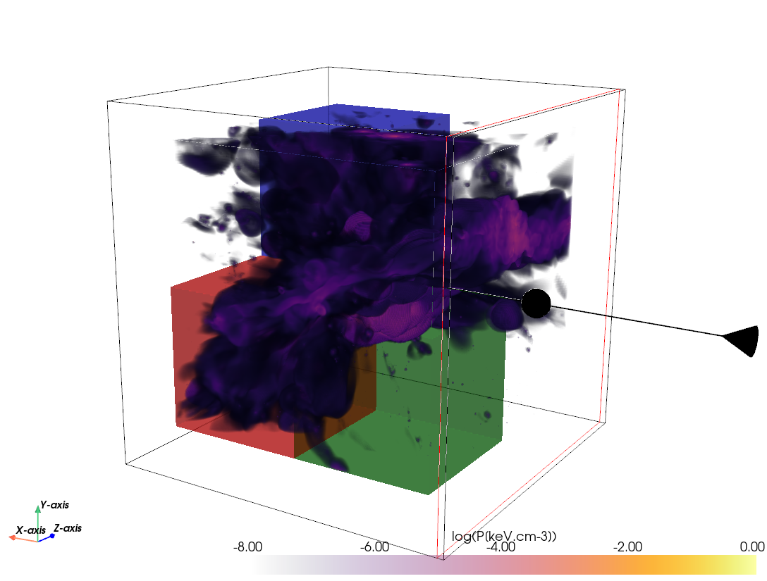
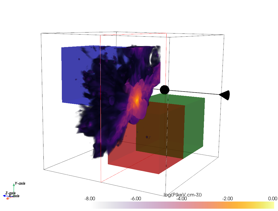
Figure 3: 3D visualisation of the pressure in Virgo replica simulation using the PyVista python library (Sullivan & Kaszynski, 2019). The pressure is in $\mathrm{keV.cm^{-3}}$, it is shown in log scale in the range [-8,0]. The top panel shows the full box, and the bottom panel shows a slice in the cluster’s core along the z-axis. The green sub-box is the region of Outflowing Material, the blue sub-box is the region of Collapsing Material, and the red sub-box is the region of Filament Material.

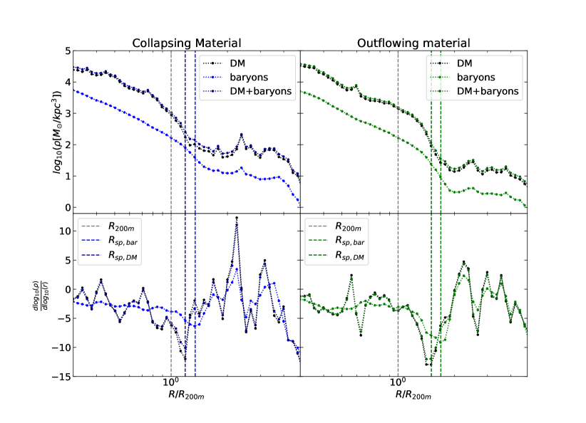
Figure 4: Comparison of radial density profiles for the Collapsing Material (left) and Outflowing Material (right). For both sides, the top panel is the density profile, and the bottom panel is the gradient. The black profile is the DM, the coloured profile (blue for Collapsing Material and green for Outflowing Material) is the baryons, and its dark counterpart is the sum of DM and baryons. Vertical dashed lines are $R_{\text{200m}}$ (grey), $R_{\text{sp}}$ from baryons (coloured) and DM (dark-coloured).

3 Splashback radius from 3D radial profiles

In this section, we identify $R_{\text{sp}}$ on 3D radial profiles. We first show the density profiles of DM, baryons, and their sum in each region and compare the values found for these quantities. We then identify $R_{\text{sp}}$ on the pressure radial profile. The values of the identified splashback radii are summarised in Table 1.

3.1 Splashback radius from 3D density profiles

We present the density profiles of DM, baryons and their sum in the regions of Collapsing Material (Fig. 4, left), Outflowing Material (Fig. 4, right), Filament Material (Fig. 5, left) and with the Full Material (Fig. 5, right). On each figure, the radial profiles are on the top sub-panel, and their gradient is on the bottom sub-panel; the profile displayed in black is the DM, and the profile displayed in light colours (respectively blue, green, red, and grey) is the baryons. Its dark-coloured counterpart is the sum of DM and baryons.

On the one hand, we clearly identify $R_{\text{sp}}$ either from DM and baryons profiles in the regions of Collapsing Material (Fig. 4, left) and Outflowing Material (Fig. 4, right). For the former, we find $R_{\text{sp,DM}}=3.4\pm 0.2\leavevmode\nobreak\$Mpc (dark-blue dashed vertical line) and $R_{\text{sp,bar}}=3.9\pm 0.2\leavevmode\nobreak\$Mpc (light-blue dashed vertical line), and for the latter we find $R_{\text{sp,DM}}=4.3\pm 0.3\leavevmode\nobreak\$Mpc (dark-green dashed vertical line) and $R_{\text{sp,bar}}=4.9\pm 0.3\leavevmode\nobreak\$Mpc (light-green dashed vertical line). Moreover, we observe that the total matter density profiles are very similar to the DM profiles. It is expected given that DM largely dominates the mass budget in clusters; consequently, we find $R_{\text{sp,tot}}=R_{\text{sp,DM}}$.

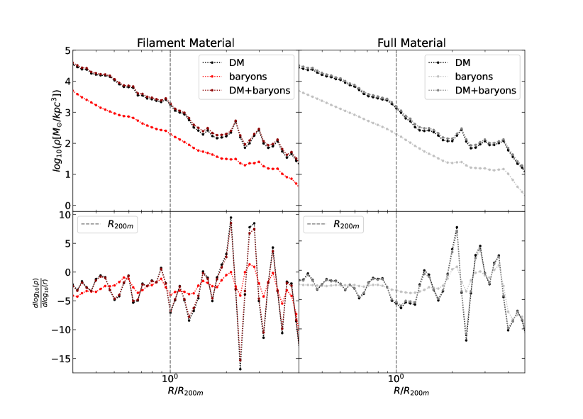
Figure 5: Comparison of radial density profiles for the Filament Material (left) and the Full Material (right). For both sides, the top panel is the density profile, and the bottom panel is the gradient. The black profile is the DM, the coloured profile (red for the Filament Material and grey for the Full Material) is the baryons, and its dark counterpart is the sum of DM and baryons. Vertical dashed lines are $R_{\text{200m}}$ (grey), $R_{\text{sp}}$ from baryons (coloured) and DM (dark-coloured).

These identified $R_{\text{sp}}$ all have different values. First, when comparing $R_{\text{sp,DM}}$ and $R_{\text{sp,bar}}$ found in the region of Collapsing (or Outflowing) Material, we observe that $R_{\text{sp,DM}}$ is about 0.5 Mpc (0.6 Mpc) smaller than $R_{\text{sp,bar}}$, that is 3.5 (2) bin width at this radius, which is quite significant. This can be explained by the fact that DM and baryons are not subject to the same physical processes; DM particles are collisionless and will thus not be slowed down while entering the cluster, whereas the baryons have viscosity and will thus be slowed down and heated while encountering the ICM.

Then, when comparing $R_{\text{sp,DM}}$ (or $R_{\text{sp,bar}}$) between the regions of Collapsing and Outflowing Material, we observe a 0.9 Mpc (1 Mpc) difference, which is very significant given it is three to four (three to five) bin width at this radius. It reflects the dynamical state in each region; in the region of Collapsing Material, there is still free-fall matter accretion, so $R_{\text{sp}}$ is located at a smaller radius than in the region of Outflowing Material where the accretion rate is much lower. This is expected and coherent with other studies (e.g., Diemer & Kravtsov 2014, O’Neil et al. 2021 and Towler et al. 2023) given that a high accretion rate induces a steeper potential well leading to a smaller $R_{\text{sp}}$. According to Towler et al. (2023), it can also be due to a high kinetic over thermal energy ratio; in our case, it might be a combination of both.

On the other hand, no clear feature is found in the gradient of either DM and baryons density profiles in the region of Filament Material (Fig.5, left) or with the Full Material (Fig.5, right). There is an important minimum on one bin at $\sim 2.4\leavevmode\nobreak\ R_{\text{200m}}$ for the DM in the region of Filament Material, but this is certainly due to the presence of a massive galaxy or a group of galaxies in the filament like all the other narrow peaks in the density profiles inducing a local maximum followed by a local minimum. Two other local minima are located close to $R_{\text{200m}}$ both for DM and baryons gradients, but they are quite weak compared to the $R_{\text{sp}}$ gradient in other regions as seen in Fig. 4. Given that, in this region, the matter is funnelled in the cluster by the filament, we are not in the case of a spherical collapse; it is thus expected not to identify $R_{\text{sp}}$. The density profiles of the Full Material are quite similar to their counterparts in the region of Filament Material. It is expected, given that this region dominates the matter budget. We can observe minima for both the baryons and DM gradient in the range [2.6,4] Mpc for DM and [2.9,4.3] Mpc for baryons. However, the gradients in this range are not as low as the minimum gradients in the regions of Outflowing and Collapsing Material. The contributions from all the regions are mixed, and its identification is thus challenging. It only yields a mean value that does not encompass the full complexity of the cluster’s dynamics.

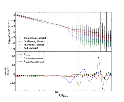
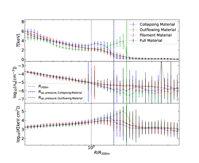
Figure 6: Left: Pressure radial profile (top) and its gradient (bottom). Right: Temperature (top), electron density (middle) and entropy (bottom) radial profiles. The colours stand for the same regions as for other figures: green for the Outlfowing Material, blue for the Collapsing Material, red for the Filament Material and black for the Full Material. $R_{\text{sp,press}}$ identified with the pressure profile with the Outflowing Material and the Collapsing Material are shown by green and blue dashed vertical lines, $R_{\text{200m}}$ is shown in grey.

3.2 Splashback radius from 3D pressure profiles

Table 1: Virgo’s characteristic radii (top) and splashback radii identified using 3D radial profiles in the regions or using the full material and 2D-projected quantities (bottom). The value gives the centre of the bin of minimum gradient; the error bars are plus and minus one bin width at this radius.

Characteristic radius (Mpc)
$R_{\text{500c}}=1.1$ Mpc	$R_{\text{200c}}=1.7\leavevmode\nobreak\$Mpc	$R_{\text{vir}}=2.1\leavevmode\nobreak\$Mpc	$R_{\text{200m}}=2.9\leavevmode\nobreak\$Mpc
Splashback radius (Mpc)
3D	DM ($R_{\text{sp,DM}}$)	Baryons ($R_{\text{sp,bar}}$)	Pressure ($R_{\text{sp,press}}$)
Collapsing Material	$3.4\pm 0.2$	$3.9\pm 0.2$	$4.3\pm 0.3$
Outflowing Material	$4.3\pm 0.3$	$4.9\pm 0.3$	$5.5\pm 0.3$
Filament Material	-	-	-
Full Material	-	-	-
2D	Surface density ($R_{\text{sp,SD}}$)	Emission measure ($R_{\text{sp,EM}}$)	Compton-$y$ ($R_{\text{sp,y}}$)
	$3.3\pm 0.2$	$3.9\pm 0.2$	$4.9\pm 0.3$

On the left panel of Fig. 6, we present the pressure radial profile (top sub-panel) and its gradient (bottom sub-panel). Similarly to Figs. 4 and 5, the profiles displayed in green, blue and red are the regions of Outflowing, Collapsing, and Filament Material, respectively, and the profile displayed in black is the Full Material. For the Full Material, we observe a peak in the pressure profile at $\sim$3.5 $R_{\text{200m}}$ associated with a massive group of galaxies already identified in Lebeau et al. (2024). Apart from this feature, we find the same results as for the DM and baryon density profiles (see Figs.4 and 5): $R_{\text{sp,press}}$ is clearly identified in the regions of Outflowing and Collapsing Material with more than one megaparsec difference whereas it is not in the region of Filament Material and for the Full Material. $R_{\text{sp,press}}=5.5\pm 0.3\leavevmode\nobreak\$Mpc in the region of Outflowing Material, and $R_{\text{sp,press}}=4.3\pm 0.3\leavevmode\nobreak\$Mpc in the region of Collapsing Material. They are highlighted by blue and green dashed vertical lines.

These radii are larger than those extracted from the baryon density profiles in those regions. However, $R_{\text{sp,press}}$ and $R_{\text{sp,bar}}$ in a given region are marginally compatible with their uncertainties. The pressure being the product of the electron density and the temperature means that this difference is due to the temperature. In fact, on the top-right panel of Fig. 6, we observe an extended temperature increase, up to a factor 1.6 in the region of Collapsing Material and a factor 6.7 in the region of Outflowing Material compared to the Full Material, which is both compatible with $R_{\text{sp,bar}}$ and $R_{\text{sp,press}}$. Multiple reasons could explain this temperature increase. First, we could have heating due to the AGN feedback, coherently with Towler et al. (2023), but it might not be powerful enough at these distances from the cluster’s core to heat the ICM gas and thus induce $R_{\text{sp,press}}$ to be hundreds of kpc further than $R_{\text{sp,bar}}$. $R_{\text{sp}}$ was originally defined from density profiles in N-body simulations. Thus, the most probable explanation is that we do not trace $R_{\text{sp}}$ with the pressure. We might rather trace accretion shocks, which is coherent with the strong temperature increase at these radii. We discuss about it in Sec. 5. Moreover, in the region of Outflowing Material, the shock in this region could be located at a larger radius in part due to the matter inflow.

In addition to the aforementioned shock fronts in the regions of Outflowing and Collapsing Materials, we notice a temperature increase, up to a factor of 1.2 in the region of Filament Material but at a much smaller radius, identified in Lebeau et al. (2024) at $\sim$850 kpc, that also indicates a shock front. This is due to the matter inflow in the filament penetrating deeply in the cluster without being slowed down and heated when encountering the ICM, as shown in recent works (e.g., Gouin et al. 2022, Vurm et al. 2023). None of these temperature increases are visible on the Full Material temperature profile because they are averaged over the overall mean temperature in each bin.

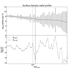
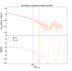
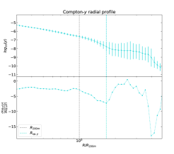
Figure 7: Projected radial profiles of Surface density (top), Emission measure (centre) and Compton-$y$ (bottom). For each quantity, the profile is shown on the top sub-panel, and its gradient is shown on the bottom sub-panel. The dashed vertical lines represent $R_{\text{200m}}$ (grey) and $R_{\text{sp}}$ (black, orange and turquoise, respectively) identified on each 2D-projected profiles extracted from the maps.

4 Splashback radius from observation-like quantities

In this section, we use observation-like quantities projected along the Virgo-Milky-Way line of sight to identify $R_{\text{sp}}$. The maps and the method used to build them are presented in Sec. 2. The 2D-projected radial profiles extracted from the maps (see again Sec. 2.2 for details) are presented in Fig. 7. The top panel is SD, the central panel is EM, and the bottom panel is $y$. On each panel, $R_{\text{200m}}$ is represented by a grey dashed vertical line. We manage to identify $R_{\text{sp}}$ on each profile; the minimum in the gradient is clearly visible before a flattening of the profile induces an increase in the gradient. Their values can be found in Table 1, and their positions are highlighted on the profiles by a dashed vertical line, respectively in black, orange, and turquoise.

When using the SD 2D-projected profile, we find $R_{\text{sp,SD}}\sim 3.3\pm 0.2$ Mpc, in agreement with the value derived from the DM density profile in the region of Collapsing Material. This value is also in the range of the minimum gradient of the DM density profile of the Full Material (see right panel of Fig. 5). However, it differs from that derived from the baryon density profile of the region of Collapsing Material. This is expected given that DM dominates the mass budget in galaxy clusters, and so does the slope of the total mass density profile, as shown in Figs. 4 and 5. Moreover, $R_{\text{sp,SD}}$ is not compatible with that found in the region of Outflowing Material, either using the DM, $R_{\text{sp,DM}}\sim 4.3\pm 0.3$ Mpc, or the baryons, $R_{\text{sp,DM}}\sim 4.9\pm 0.3$ Mpc, density profile. The slope steepening of the radial profile that we associate with $R_{\text{sp}}$ extends over at least one order of magnitude on the DM profiles. Therefore, the steepening at the lowest radius among the regions determines that of the SD radial profile; it explains the agreement with the value found in the region of Collapsing Material. We can conclude that, in our case and in agreement with other works (e.g., Towler et al., 2023), when using SD map to identify $R_{\text{sp}}$, we trace the DM dynamics in the region Collapsing Material.

The Emission measure traces the gas density as it is the integral of the electron density times the proton density. We find $R_{\text{sp,EM}}\sim 3.9\leavevmode\nobreak\ \pm 0.2$ Mpc, which is, this time, in agreement with the value derived from the baryons density profile in the region of Collapsing Material. This is also expected, given that EM traces the gas density. Once again, the steepening at the lowest radius among the regions, the region of Collapsing Material in our case, determines that of the EM radial profile. The EM is thus a tracer of the gas dynamics in the region of Collapsing Material.

Finally, the tSZ effect traces the pressure distribution; we find $R_{\text{sp,yc}}\sim 4.9\pm 0.3$ Mpc on the $y$ 2D-projected radial profile, which is much more distant from the centre than its SD and EM counterparts. It is in between the values extracted from the pressure profiles in the regions of Outflowing and Collapsing Material. We would expect that $R_{\text{sp}}$ extracted from this 2D-projected profile agrees with that extracted from the pressure profile in the region of Collapsing Material, similarly to EM and SD. The low-pressure area visible on the left part of the map, inducing a substantial $y$ intensity decrease, is located in the region of Outflowing Material and undoubtedly impacts $R_{\text{sp}}$ identification. The contribution of the regions of Outflowing and Collapsing Material seems then to be more mixed on this 2D-projected $y$ profile than on the SD and EM profiles due to this almost-empty region; it is another projection effect. The $y$ map traces the projected pressure distribution and gives much larger $R_{\text{sp}}$ than the SD and EM maps. However, it is still compatible with $R_{\text{sp,bar}}$ and $R_{\text{sp,press}}$ identified in the region of Outflowing Material.

5 Discussion

In this work, we used DM density, baryons density (and their sum) and pressure radial profiles to identify $R_{\text{sp}}$. We also used projected observation-like quantities comparable to the aforementioned 3D profiles. We found different values ranging from 3.3 Mpc to 5.5 Mpc; we compare them in Fig. 8. It shows that $R_{\text{sp,DM}}$, considered as the reference value since $R_{\text{sp}}$ was defined from DM simulations, has the smallest value in each region. $R_{\text{sp,bar}}$, and $R_{\text{sp,press}}$ even more, overestimates $R_{\text{sp}}$ compared to the $R_{\text{sp,DM}}$ reference value. However, as discussed above, it is coherent since DM is collisionless. In contrast, baryons have viscosity, and $R_{\text{sp,press}}$ might rather be an accretion shock, as we discuss in more detail below. Moreover, the radius found by each tracer is always at smaller radii in the region of Collapsing Material than in the region of Outflowing Material, which is consistent with other works (e.g., Towler et al., 2023) since the former region has a higher accretion rate leading to a steeper gravitational potential well. Finally, $R_{\text{sp}}$ identified from 2D-projected radial profiles of SD, EM, and $y$ are in quite good agreement with their 3D counterpart (i.e. DM for SD, baryons for EM and pressure for $y$) in the region of Collapsing Material. Figure 8 thus highlights how much the identified $R_{\text{sp}}$ depends on the accretion regime in a given region and the probe used to identify it.

Other works (e.g., More et al., 2016; Chang et al., 2018; Shin et al., 2019; Adhikari et al., 2021; Bianconi et al., 2021; Rana et al., 2023) used galaxy number density to identify $R_{\text{sp}}$. Pizzardo et al. (2023) also proposed to define $R_{\text{sp}}$ as the transition point from concave to convex shape, i.e. second derivative equal to zero, of the radial profile of galaxy radial velocities. Regardless of the method used, these works must stack over a sample of clusters to increase the signal-to-noise ratio and reach a smooth enough radial profile to reliably identify $R_{\text{sp}}$. In our case study, we cannot apply the same technique because we only consider a single cluster. The detection of $R_{\text{sp}}$ from the galaxy number density or radial velocity profile was not possible in our case study; the profiles were too noisy due to the limited number of resolved galaxies in the cluster. On the observational side, given that Virgo is located in our direct vicinity, at approximatively 16 Mpc (Mei et al., 2007), comprehensive study of its galaxy population (e.g., the Next Generation Virgo Cluster Survey Ferrarese et al. 2016 or the Virgo Environmental Survey Tracing Ionised Gas Emission Boselli et al. 2018 surveys) were carried out. We could thus derive its projected galaxy density or the galaxy radial velocities, but similarly to the present work, the limited number of detected galaxies in this mid-mass cluster, $M_{\text{vir}}\sim 6\times 10^{14}\leavevmode\nobreak\ \mathrm{M_{\odot}}$ (Lebeau et al. 2024 and references therein), could prevent the identification of $R_{\text{sp}}$ from galaxies.

Using 3D DM radial profiles (or the sum of DM and baryons) to identify $R_{\text{sp}}$ as originally done by Diemer & Kravtsov (2014), we trace the distinct matter dynamics in each region. In particular, when using the SD 2D-projected radial profile, we trace the matter dynamics in the region of Collapsing Material since this region drives the radial profile shape. It is because its slope steepening occurs at a smaller radius than in the region of Outflowing Material due to the steeper potential well induced by the higher accretion rate. If we relate it to the observed Virgo cluster, which is very extended in the sky ($R_{\text{vir}}$ angular size of 4°; see e.g. Planck Collaboration, 2016), deriving its mass surface density would be very challenging as it would necessitate a dedicated observation program and enough luminous background sources to build a faithful lens model. To our knowledge, it has not been done so far; at best, galaxy-galaxy lensing could be performed in Virgo (Ferrarese et al., 2012). For other individual clusters, it might be possible to build a cluster lens model up to $R_{\text{sp}}$ provided there are sufficiently luminous and extended background sources.

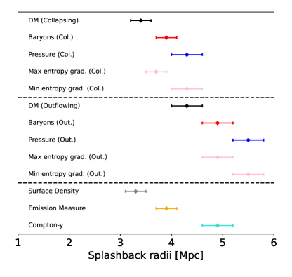
Figure 8: Comparison of the splashback radii obtained in this work. The values can be found in Tab. 1. In addition, the minimum and maximum gradient of entropy are shown in pink.

When 3D baryons radial profiles are used to identify $R_{\text{sp}}$, we trace the baryons thermodynamics in each region. Moreover, $R_{\text{sp,bar}}$ is significantly larger than $R_{\text{sp,DM}}$, multiple bin width, because baryons have viscosity whereas DM is collisionless. We used the 2D-projected profiles of the EM to trace baryon thermodynamics in an observation-like context. Similarly to SD for DM, we find that EM traces the thermodynamics in the region of Collapsing Material as this region drives the radial profile shape. In reality, observing Virgo’s $R_{\text{sp}}$, or any other cluster, in the X-rays would be arduous too because the surface brightness is proportional to the squared density, leading to a very faint signal in the outskirts. As a matter of fact, Urban et al. (2011), with XMM-Newton, and Simionescu et al. (2015), with Suzaku, observed Virgo beyond $R_{\text{200c}}$ but only in particular arms using mosaics. The recently launched XRISM telescope (XRISM Science Team, 2020; Tashiro, 2022) will not be able to study Virgo’s outskirts due to its small collecting area; it will rather focus on bright region Virgo where M87 is located. Recently, McCall et al. (2024) took advantage of the SRG/eRosita all-sky survey to study the Virgo cluster up to 3 Mpc. It is unprecedented, still it does not reach the radii at which we identified $R_{\text{sp}}$ in this work, given they are all beyond 3 Mpc (see Tab. 1). However, they conducted an azimuthal study similar to that performed both in observations (e.g., Ettori et al., 1998; Vikhlinin et al., 1999; Gouin et al., 2020) and simulations Gouin et al. (2022), and they probed an extended ICM emission and a cold front. With dedicated programs in the future, we might be able to conduct region studies at large radii like ours with observation data.

The third tracer used to identify $R_{\text{sp}}$ in the literature, and hence investigated in this work, is the gas pressure. Similarly to DM and baryon density, we identify $R_{\text{sp,press}}$ in the regions of Collapsing and Outlowing Material but at much larger radii. However, $R_{\text{sp}}$ is defined as a dynamical boundary; it is thus supposed to be identified from radial density profiles as it traces the underlying gravitational potential well driving particles’ velocity. The gas in the ICM experiences much more complex physical processes than DM, such as heating and turbulence due to AGN and SN feedback or shocks, particularly in the cluster’s outskirts where cosmic matter is accreted and shocked while entering the ICM. Therefore, when identifying the radius of steepest slope on pressure radial profiles, we might identify an accretion shock rather than $R_{\text{sp}}$. Some work based on simulations (e.g., Shi, 2016; Towler et al., 2023) find a good agreement between the accretion shock radius, $R_{\text{sh}}$, and $R_{\text{sp}}$ whereas Aung et al. (2021) find a ratio $R_{\text{sh}}/R_{\text{sp}}\sim$1.89 where $R_{\text{sp}}$ is defined from DM particles trajectories and $R_{\text{sh}}$ is defined as the radius of the minimum in the slope of the entropy profile. Moreover, Anbajagane et al. (2022) identify two minima on the stacked pressure profile of clusters observed with the South Pole Telescope (SPT; Plagge et al. 2010). They associate the first one with a non-thermal equilibrium between ions and electrons occurring around shocks, as kinetic energy is better converted to thermal energy by ions than electrons given they are more massive. However, this minimum cannot be observed and confirmed in our simulation since we assume local thermal equilibrium between ions and electrons. Anbajagane et al. (2022) identify the second minima to be related to an accretion shock front for which they define a lower limit of $R_{\text{sh}}/R_{\text{sp}}\sim$2.16$\pm$0.59. For simplicity, in the present work, we noted the minimum in the pressure gradient $R_{\text{sp,press}}$ but in fact, the ratio $R_{\text{sp,press}}/R_{\text{sp,DM}}$ (similar to $R_{\text{sh}}/R_{\text{sp}}$ in Aung et al. (2021)) is roughly 1.28 in the region of Outflowing Material and 1.26 in the region of Collapsing Material. It is a bit higher than one but much lower than the ratios found by Aung et al. (2021) and Anbajagane et al. (2022). Consequently, we are not able to state if $R_{\text{sh}}$ is distinguishable from $R_{\text{sp}}$ using the $R_{\text{sp,press}}/R_{\text{sp,DM}}$ ratio in our case study, although the temperature increase at these radii tends to motivate the presence of an accretion shock.

In addition, when identifying $R_{\text{sp}}$ on $y$ 2D-projected profile, its position is between $R_{\text{sp,press}}$ found in the regions of Collapsing and Outflowing Material due to a strong projection effect, making the use and interpretation of this tracer even more challenging. Finally, when considering the tSZ effect, Virgo was only observed by the Planck telescope (Planck Collaboration, 2016); the SPT and ACT ground telescopes cannot observe Virgo as it is close to the North Pole. Due to its proximity, Virgo has the largest integrated tSZ flux (Taylor et al., 2003), so it would be the best target for a first detection of $R_{\text{sp}}$ in a single cluster. Moreover, the tSZ effect is the integrated pressure along the line of sight so it is proportional to electron density, whereas the surface brightness in the X-rays is proportional to the squared density, allowing to study the ICM in the outskirts. However, Planck Collaboration (2016) only studied Virgo up to $\sim$1 Mpc, which would not be enough to identify $R_{\text{sp,press}}$. Future sub-mm experiments such as LiteBIRD (LiteBIRD Collaboration, 2023) might be able to observe clusters outskirts up to $R_{\text{sp}}$.

Other thermodynamic quantities could be used as tracers of $R_{\text{sp}}$; for instance, it may, in principle, be possible to identify it from electron density profiles. In our case, we could not identify $R_{\text{sp}}$ on any of the electron density profiles (see middle-right panel of Fig. 6). Still, for the regions of Outflowing and Collapsing Material they seem to agree with their pressure counterparts since the steepening before the flattening of the profile occurs in the same range. Finally, the entropy, defined as $K=T/n_{e}^{2/3}$, is a tracer of the thermalisation state of the gas after being heated via shocks or adiabatic compression (see Tozzi et al. 2000 for detection of entropy and Markevitch & Vikhlinin 2007 for a review on shocks). Both Aung et al. (2021) and Towler et al. (2023) searched for the minimum gradient of the entropy profile to identify the accretion shock radius, as discussed earlier. Towler et al. (2023) also found the maximum entropy gradient at approximately the splashback radius when defined from gas density profile; which is quite expected since when there is a minimum in the gas density gradient, there should be a corresponding maximum in the entropy gradient. In our work, in the regions of Outflowing and Collapsing Material, the minimum gradient is at the same radius as $R_{\text{sp,press}}$ and the maximum approximately at the same radius as $R_{\text{sp,bar}}$ (see Max and Min entropy grad. lines, displayed in pink, in Fig. 8). This would tend to show that $R_{\text{sp,press}}$ is an accretion shock, even if, as already discussed, we cannot confirm it from the $R_{\text{sp,press}}/R_{\text{sp,DM}}$ ratio. Anyway, the entropy seems to be a tracer of both $R_{\text{sp}}$ and $R_{\text{sh}}$.

We chose as a baseline of our analysis to compute the mean pressure and 2D-projected radial profiles. Computing the median profiles is a better tracer of an average quantity for log-normal distributions, which can be the case for the ICM properties in observations (see e.g., Zhuravleva et al., 2013; Eckert et al., 2015). In our case, given that we have selected the ionised gas cells (see Sect. 2), that we have a very high number of cells per bin and that the pressure is a quite smoothly distributed quantity, using the median instead of the mean gives quite similar results for 3D pressure profiles (see Fig. 9 in Appendix A) and for $y$ 2D-projected profiles (see bottom panel of Fig. 10 in Appendix B). However, the SD intensity in pixels is not gaussian-distributed. Indeed, there are important density contrasts due to substructures. Therefore, the median 2D-projected profile (see top panel of Fig. 10 in Appendix B) is quite different from its mean counterpart. Particularly, there is an important dip within $R_{\text{200m}}$ causing a very important gradient. Though we doubt it can be associated with $R_{\text{sp}}$ at such a low radius, it rather emphasises the transition from the halo-dominated region to the background-dominated one. For EM, the median profile (see middle panel of Fig.10 in Appendix B) is consistent with the mean profile, including its gradient, up to $R_{\text{sp,EM}}$ but then gets steeper, so its minimum gradient is located few bins further. In this case, we are not able to conclude if it is due to the temperature cut, a projection effect or if the median really identifies $R_{\text{sp,EM}}$ at a larger radius, moreover because the EM pixel distribution is not log-normal. In conclusion, even more caution is required when identifying $R_{\text{sp}}$ from EM and SD since the method used to compute the radial profile has a significant impact.

We have shown that $R_{\text{sp}}$, more precisely the minimum in the gradient of a radial profile, seems to be more a tracer of the dynamical state of a cluster component (DM or baryons) in a given region than an observable natural cluster boundary. However, our work suffers one major limitation since it is a case study of a particularly disturbed cluster while other cited works conducted statistical studies; our conclusions are thus not to be taken as universal. Yet this first case study of $R_{\text{sp}}$ in regions of a highly-refined zoom-in simulation highlights how complex a single cluster can be. It also shows that when generalising over a cluster sample we mainly get a mean value averaging the signals in all the cluster environments. Specifically, when stacking over a large cluster sample, the resulting signal is averaged out, which smooths the outskirts, not enabling to identify $R_{\text{sp}}$ (e.g., see the stacking of 100 random projections of Virgo on Fig. 10 in Appendix B). Our case study is thus complementary to statistical studies where they tested the dependence of $R_{\text{sp}}$ on other parameters such as cluster mass, accretion rate or redshift (Adhikari et al., 2014; Diemer & Kravtsov, 2014; More et al., 2015; Diemer et al., 2017; Mansfield et al., 2017; O’Neil et al., 2021).

6 Conclusion

In this work, we identified the splashback radius, $R_{\text{sp}}$, i.e. the minimum in the gradient of the radial profile, using the radial density profiles of DM, baryons, or their sum as well as pressure in regions of the simulated Virgo replica. These different regions, which contain outflowing, collapsing, and fragmented material, represent dynamical states occurring simultaneously in our Virgo case study. We then built projected maps of surface density, emission measure, and Compton-$y$ along the Virgo-Milky Way line of sight in our constrained simulation of the Local Universe. In addition, we discussed the use of different tracers to investigate $R_{\text{sp}}$; in particular, the pressure could rather be a tracer of an accretion shock than $R_{\text{sp}}$. We also discussed their potential detectability for a single cluster like Virgo, using median profiles instead of mean profiles to identify $R_{\text{sp}}$. We pointed out that our conclusions about this particularly disturbed cluster are not to be taken as universal, although this case study is complementary to statistical studies.

We found that $R_{\text{sp}}$, when its identification is possible, varies of $\sim$1 Mpc between regions for a given quantity, which is about three to four bin widths at this radius. We also found that in the same region, there is almost a 0.5 Mpc difference between the splashback radius extracted from the baryons density profile and that extracted from the DM density profile, so 2 to 3 bin width, which is expected given that these components of galaxy clusters (i.e. baryons or DM) do not follow the same physical processes. Moreover, we notice that the contributions of all the regions are mixed when using the matter in the full zoom-in box to identify $R_{\text{sp}}$, not allowing us to identify it clearly.

When extracting the splashback radius from 2D-projected profiles of SD, EM and $y$, we also found that each traces the physics processes of their underlying component. Moreover, the identified splashback radii are more in agreement with those found in the region of Collapsing Material than that of Outflowing Material. It is certainly because the slope steepening in this region determines that of the projected profile given that it is located at a smaller radius than in the other regions. Except for the Compton-$y$ profile, for which there is a consequent projection effect.

This study of regions in this simulated Virgo cluster shows the complex and various dynamics of clusters’ outskirts and their impact on the splashback radius estimate. Caution is thus required when using the splashback radius as a natural boundary of clusters, especially for a complex cluster, as we have demonstrated for Virgo, and when stacking.

Appendix A Comparison of median and mean pressure radial profiles in the regions of Collapsing and Outlowing Material

Fig. 9 compares the mean (light profiles) and median (dark profiles) pressure radial profiles in the regions of Collapsing (blue and dark blue) and Outflowing Material (green and dark green). It shows that using the median instead of the mean to identify $R_{\text{sp}}$ gives the same result in the region of Outflowing Material. In the region of Collapsing Material, $R_{\text{sp}}$ is identified at a smaller radius on the median profile but still in agreement with that identified on the mean profile given the uncertainties. However, the median profiles have a steepening of their profile occurring at a smaller radius, although the median and the mean profiles are at less than 2$\sigma$ from each other at worst.

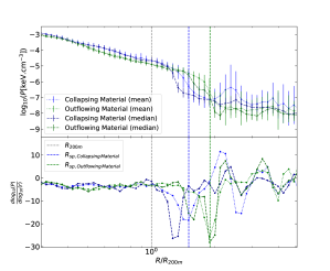
Figure 9: Pressure radial profiles in the regions of Collapsing (blue for the mean and dark blue for the median) and Outflowing Material (green for the mean and dark green for the median). The vertical dashed lines are $R_{\text{sp,\,Collapsing\,Material}}$ (blue), $R_{\text{sp,\,Outflowing\,Material}}$ (green) and $R_{200m}$ (grey).

Appendix B 2D-projected radial profiles of 100 stacked random projections compared to the mean and median profile of one projection

In Fig.10, we present SD (top), EM (middle) and $y$ (bottom) 2D-projected radial profiles of 100 stacked random projections, respectively in light-red, dark-red and dark-blue. The simulation box was rotated using randomly chosen angles to create 100 projections from which we computed the maps and derived the 2D-projected mean profiles following the method presented in Sect.2. We then calculated the average profile over the hundred realisations. For comparison, we also show 2D-projected mean (black, red and turquoise, respectively) and median (grey, orange and green, respectively) radial profiles. It shows that the stacked profile tends to have a higher signal in the outskirts than the mean or median profiles from the projection (named Cen on the figures) used in this work. It is expected because the filaments have various orientations in the random projections, leading to a smoothed stacked profile. We thus cannot identify $R_{\text{sp}}$ on any of these stacked 2D-projected profiles. We discuss the differences between the mean and median profiles in Sec.5.

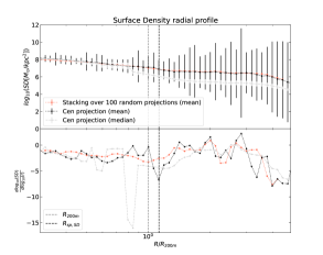
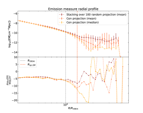
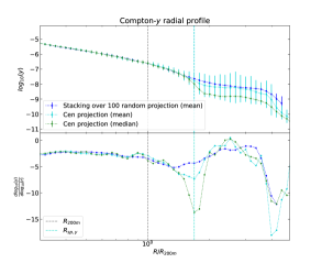
Figure 10: SD (top), EM (middle) and $y$ (bottom) 2D-projected radial profiles of 100 stacked random projections, respectively in brown, dark-red and dark-blue. For comparison, we also show 2D-projected mean (resp. in dark, red and cyan) and median (resp. in grey, orange and light-blue) radial profiles. For the three figures, the vertical dashed lines are $R_{\text{200m}}$ (grey) and $R_{\text{sp}}$ (respectively in black, red and cyan)