Improving efficiency of parallel across the method spectral deferred corrections

Abstract

Parallel-across-the method time integration can provide small scale parallelism when solving initial value problems. Spectral deferred corrections (SDC) with a diagonal sweeper, which is closely related to iterated Runge-Kutta methods proposed by Van der Houwen and Sommeijer, can use a number of threads equal to the number of quadrature nodes in the underlying collocation method. However, convergence speed, efficiency and stability depends critically on the used coefficients. Previous approaches have used numerical optimization to find good parameters. Instead, we propose an ansatz that allows to find optimal parameters analytically. We show that the resulting parallel SDC methods provide stability domains and convergence order very similar to those of well established serial SDC variants. Using a model for computational cost that assumes 80% efficiency of an implementation of parallel SDC we show that our variants are competitive with serial SDC, previously published parallel SDC coefficients as well as Picard iteration, explicit RKM-4 and an implicit fourth-order diagonally implicit Runge-Kutta method.

65R20, 45L05, 65L20

1 Introduction

Numerical methods to solve initial-value problems for nonlinear systems of ordinary differential equations (ODEs)

(1) $$\frac{du(t)}{dt}=f(t,u(t)),\quad t\in[0,T],\quad u(0)=u_{0}\in\mathbb{R}^{N_{\text{dof}}},$$

are of great importance for many domain sciences. For ODEs arising from spatial discretization of a partial differential equation in a method-of-lines approach, the number of degrees of freedom $N_{\text{dof}}$ is often very large. Hence, developing efficient methods to minimize time-to-solution and computational cost becomes important. Because of the large number of compute cores in modern computers, leveraging concurrency is one of the most effective ways to reduce solution times.

A widely used class of methods for solving (1) are Runge–Kutta Methods (RKM), usually represented by Butcher tables of the form

$$\begin{array}[]{c|c}\boldsymbol{c}&\mathbf{A}\\ \hline\cr\\[-10.00002pt] &\boldsymbol{b}^{\top}\end{array}$$

with $\mathbf{A}\in\mathbb{R}^{s\times s}$, $\boldsymbol{b},\boldsymbol{c}\in\mathbb{R}^{s}$, and $s$ the number of stages. The Butcher table is a concise way to represent the update from $t_{0}$ to $t_{0}+\Delta t$, which, for a scalar ODE, reads

(2) solve: $$u(\boldsymbol{t}_{s})-\Delta t\mathbf{A}f(\boldsymbol{t}_{s},u(\boldsymbol{t}_{s}))=u(t_{0}\boldsymbol{\mathds{1}}),\quad\boldsymbol{t}_{s}=t_{0}\boldsymbol{\mathds{1}}+\Delta t\boldsymbol{c},$$

(3) update: $$u(t_{0}+\Delta t)=u(t_{0})+\Delta t\boldsymbol{b}^{\top}f(\boldsymbol{t}_{s},u(\boldsymbol{t}_{s})),$$

where $\boldsymbol{\mathds{1}}=(1,\dots,1)^{\top}$ is the vector with unit entries and $u(\boldsymbol{t}_{s})$ is the vector containing solutions at all times in $\boldsymbol{t}_{s}$ (same notation used for $f$). For a system of ODEs, the same idea applies to every degree of freedom at the same time. Thus, for implicit Runge–Kutta methods (IRK) where the matrix $\mathbf{A}$ is dense, computing the stages (2) requires solving a system of size $sN_{\text{dof}}\times sN_{\text{dof}}$.

A popular class of IRK are collocation methods [14, Sec II.7] based on Gaussian quadrature. Collocation methods are attractive since they can be of very high order and are A-stable or L-stable depending on the used type of quadrature nodes. However, since they have a dense matrix $\mathbf{A}$, they are computationally expensive if $N_{\text{dof}}$ is large. Diagonally implicit Runge-Kutta methods (DIRK) with a lower-triangular $\mathbf{A}$ are computationally cheaper as the implicit systems for the stages can be solved independently. However, compared to collocation, DIRK methods have lower order for equal number of stages and typically come with less favorable stability properties.

1.1 Parallelism across the method

First ideas to exploit parallelism in the numerical solution of ODEs emerged in the 1960s [25]. Given the massive increase in concurrency in modern high-performance computing, the last two decades have seen a dramatic rise in interest in parallel-in-time methods, see the recent reviews by Ong and Schroder [28] or Gander [11]. In the terminology established by Gear [12], we focus on a “parallelism across the method” where a time integration scheme is designed such that computations within a single time step can be performed in parallel. By contrast, “parallel across the steps” methods like Parareal [23], PFASST [8] or MGRIT [9] parallelize across multiple time steps. Revisionist integral deferred corrections (RIDC) are a hybrid that compute a small number of time steps simultaneously [27].

For collocation methods, parallel across the method variants exist based on diagonalization of $\mathbf{A}$  [3, 26, 22, 29, 38] or based on using a specific GMRES preconditioning [30, 21, 24]. However, those approaches can introduce significant overhead and, in particular for large problems, struggle to outperform sequential time-stepping [4]. Runge-Kutta methods with parallelism across stages or blocks of stages, that is with diagonal or lower block diagonal Butcher matrices, have also been considered but the resulting schemes lack stability and are of lower order than their sequential counterparts [18, 17, 19, 31, 36].

Spectral deferred correction (SDC), introduced in 2000 by Dutt et al. [7], are an iterative approach for computing the stages of a collocation method by performing multiple “sweeps” through the quadrature nodes with a lower order method. SDC can also be interpreted as a preconditioned fixed-point or Richardson iteration [16, Sec. 3]. In standard SDC, the preconditioner applied to (2) corresponds to a lower triangular matrix that is inverted by forward substitution, giving rise to the sweep-like style of iterations. Speck [38] suggests the use of diagonal preconditioner instead, which allows to parallelize the iteration update for the stages. However, depending on the entries of the diagonal preconditioner, convergence of parallel SDC can be much slower than convergence of standard SDC. Unbeknownst to the author, this idea had been proposed before by van der Houwen & Sommeijer [43] but in the context of iterated IRK methods instead of SDC.

We show in §2.1 that SDC can be interpreted as an iterated RKM with a specific lower-triangular preconditioner, however, this link has not yet been made in the literature before. Also referred to as RKM based on predictor-corrector formula, iterated IRK have been widely studied in the 1990s and have been shown to preserve important attributes of the underlying collocation method such as order and stability if enough iterations are performed [2]. They form the basis for the “Parallel iterated RK across the steps” (PIRKAS) methods [42, 41, 33], which can be written as Block Gauss-Seidel SDC (BGS-SDC) methods [13, 1]. Both PIRKAS and BGS-SDC methods have been combined with parallelism across the method using diagonal preconditioning [43] to form the Parallel Diagonal-implicitly Iterated RK Across the Steps (PDIRKAS) methods [15, 40, 37, 45, 46], allowing two levels of parallelism in time. Similar two-level parallelism in time has been achieved by a combination of PFASST [8] with parallel SDC [35].

The key for fast convergence and thus good performance of either parallel SDC or iterated IRK is the choice of coefficients in the diagonal preconditioner [43, Sec. 3]. The authors identify two possible optimization problems to compute good diagonal coefficients suited for either non-stiff and stiff problems. Both problems seek to minimize the spectral radius of certain matrices but since those are ill conditioned, most optimization algorithms struggle as the number of parallel stages $s$ increases. This was already acknowledged by both van der Houwen & Sommeijer and Speck [43, 38], and van der Houwen & Sommeijer proposed to use an objective function based on the stability function of the iterated IRK to remedy this issue. However, this approach was only suitable for stiff problems, and only applicable to a few types of IRK methods.

1.2 Contributions

We present a generic approach for computing optimized coefficients for diagonal preconditioning in SDC or iterated IRK that is suited for both stiff and non-stiff problems. This approach leads to three sets of coefficients that we call MIN-SR-NS, MIN-SR-S and MIN-SR-FLEX. While MIN-SR-NS is suited for non-stiff problems, MIN-SR-S and MIN-SR-FLEX are designed for stiff problems. We provide an analytical expression for the coefficients of MIN-SR-NS and MIN-SR-FLEX, and a generic approach to generate MIN-SR-S coefficients for any type of collocation method. We show that the resulting SDC methods provide accurate and stable parallel time-integration schemes when compared to state-of-the art SDC preconditioners, in particular those provided by van der Houwen & Sommeijer [43] or Weiser [47]. We demonstrate that optimized parallel SDC methods can compete with respect to computational cost against standard RKM from the literature because their design allows to exploit parallelism across the method without sacrificing speed of convergence. All numerical experiments reported in this paper can be reproduced with the accompanying code [39].

2 Optimal diagonally preconditioned Spectral Deferred Corrections

We start by giving a concise description of SDC in §2.1 and develop the new diagonal preconditioners in §2.2. For details on SDC see Dutt et al. or Huang et al. [7, 16].

2.1 Spectral Deferred Corrections as a fixed point iteration

Consider the Picard formulation of the initial value problem (1) on $[t_{0},t_{0}+\Delta t]$

(4) $$u(t)=u_{0}+\int_{t_{0}}^{t}f(s,u(s))ds.$$

for some time step size $\Delta t$. Choosing $M\in\mathbb{N}$ collocation nodes $0\leq\tau_{1}<\dots<\tau_{M}\leq 1$, and defining $t_{m}=t_{0}+\tau_{m}\Delta t$, we can write (4) for each $t_{m}$ as

(5) $$u(t_{m})=u_{0}+\Delta t\int_{0}^{\tau_{m}}f(t_{0}+s\Delta t,u(t_{0}+s\Delta t))ds,\quad m=1,\dots,M.$$

Let $\ell_{i}$ denote the $i^{\rm{th}}$ Lagrange polynomial associated to the nodes $\tau_{1},\dots,\tau_{M}$. Using a polynomial approximation of the integrand $f$ turns (5) into

(6) $$u_{m}=u_{0}+\Delta t\sum_{i=1}^{M}\left(\int_{0}^{\tau_{m}}\ell_{i}(s)ds\right)f(t_{i},u_{i}),\quad m=1,\dots,M,$$

where $u_{m}$ is a discrete approximation of $u(t_{m})$. We collect (6) for $m=1,\ldots,M$ in the compact matrix formulation

(7) $$\boldsymbol{u}-\Delta t\mathbf{Q}f(\boldsymbol{u})=u_{0}\boldsymbol{\mathds{1}},$$

with $\boldsymbol{u}=[u_{1},\dots,u_{M}]^{\top}$, $f(\boldsymbol{u})=[f(t_{1},u_{1}),\dots,f(t_{M},u_{M})]^{\top}$, $\boldsymbol{\mathds{1}}=[1,\dots,1]^{\top}$. The collocation matrix $\mathbf{Q}\in\mathbb{R}^{M\times M}$ has entries

(8) $$[\mathbf{Q}]_{ij}=\int_{0}^{\tau_{i}}\ell_{j}(s)ds.$$

We refer to (7) as the collocation problem. This is equivalent to the first RKM step (2) since the collocation method is an IRK method with $\mathbf{A}=\mathbf{Q}$, $[\boldsymbol{b}]_{i}=\int_{0}^{1}\ell_{i}(s)ds$ and $[\boldsymbol{c}]_{i}=\tau_{i}$ [14, Th. 7.7]. The second RKM step (3) is equivalent to the update

(9) $$u(t_{0}+\Delta t)\approx u_{0}+\boldsymbol{b}^{\top}f(\boldsymbol{u}).$$

Note that if $\tau_{M}=1$ one can simply bring forward the solution at the last quadrature node and set $u(t_{0}+\Delta t)\approx u_{M}$ instead. The node distribution defines the accuracy order of the collocation method [43, Tab. 2.1] with Gauss-Lobatto (Lobatto) nodes producing a method of order $2M-2$ and Gauss-Radau IIA nodes (Radau-Right) a method of order $2M-1$.

SDC solves (7) with a preconditioned fixed-point iteration

(10) $$\boldsymbol{u}^{k+1}=\boldsymbol{u}^{k}+\mathbf{P}^{-1}\left[u_{0}\boldsymbol{\mathds{1}}-\left(\boldsymbol{u}^{k}-\Delta t\mathbf{Q}f(\boldsymbol{u}^{k})\right)\right],$$

where $\mathbf{P[\boldsymbol{u}]}:=\boldsymbol{u}-\Delta t\mathbf{Q}_{\Delta}f(\boldsymbol{u})$ and $\mathbf{Q}_{\Delta}\in\mathbb{R}^{M\times M}$ is a matrix called the SDC preconditioner. Because $\mathbf{Q}_{\Delta}$ is typically chosen to be lower triangular, the inversion of $\mathbf{P}$ can be done by forward substitution which proceeds node by node. Hence an SDC iteration is often called a “sweep”. The generic form of an SDC sweep is

(11) $$\boldsymbol{u}^{k+1}-\Delta t\mathbf{Q}_{\Delta}f(\boldsymbol{u}^{k+1})=u_{0}\boldsymbol{\mathds{1}}+\Delta t(\mathbf{Q}-\mathbf{Q}_{\Delta})f(\boldsymbol{u}^{k}).$$

By setting $\mathbf{Q}_{\Delta}=0$ we retrieve the classical Picard iteration (PIC). The original SDC method [7] considers $\mathbf{Q}_{\Delta}$ matrices based on explicit (EE) and implicit Euler (IE)

$$\mathbf{Q}_{\Delta}^{\texttt{EE}}=\begin{bmatrix}0&0&\dots&0&0\\ \Delta\tau_{2}&0&\dots&0&0\\ \vdots&\vdots&\ddots&\vdots&\vdots\\ \Delta\tau_{2}&\Delta\tau_{3}&\dots&\Delta\tau_{M}&0\end{bmatrix},\quad\mathbf{Q}_{\Delta}^{\texttt{IE}}=\begin{bmatrix}\Delta\tau_{1}&0&\dots&0\\ \Delta\tau_{1}&\Delta\tau_{2}&\dots&0\\ \vdots&\vdots&\ddots&\vdots\\ \Delta\tau_{1}&\Delta\tau_{2}&\dots&\Delta\tau_{M}\end{bmatrix},$$

where $\Delta\tau_{m}=\tau_{m}-\tau_{m-1}$ for $1\leq m\leq M$, and $\tau_{0}=0$. The computational cost of solving (11) with forward substitutions is the same as that of a DIRK method with $s=M$ stages.

Remark 2.1.

Performing the update (9) improves the order of the step solution but can also reduce numerical stability [34, Rem. 4]. This is also confirmed by numerical experiments not presented here, as some preconditioning that appears to be $A$-stable can loose this property when performing the collocation update. While this aspect would need further investigation, it motivates us to only use node distributions with $\tau_{M}=1$ (i.e., Radau-Right and Lobatto) to avoid doing (9) for better numerical stability.

Remark 2.2.

We can also define the SDC sweep based on the $\mathbf{A}$ and $\boldsymbol{c}$ Butcher arrays of a DIRK method: selecting $\mathbf{Q}_{\Delta}=\mathbf{Q}=\mathbf{A}$ allows to retrieve (2) from (11), independent of $\boldsymbol{u}^{0}$, and performing the collocation update (9) is equivalent to the RKM update (3). Hence, any generic SDC implementation based on (11) can be used to run any type of DIRK (or ERK) method, provided some minor code optimizations. Such an approach is currently implemented in pySDC [39].

As first suggested by Speck [38], it is also possible to use a diagonal $\mathbf{Q}_{\Delta}$. This allows to compute the sweep update for each node in parallel using $M$ threads or processes, in the same way as for PIC where $\mathbf{Q}_{\Delta}=0$. Note also that if we consider any IRK method with a dense Butcher matrix $\mathbf{A}$, then the diagonal preconditioned iteration on the first RKM step (2) introduced by van der Houwen & Sommeijer [43, Eq. 3.1a] is equivalent to the generic SDC sweep (11) with a diagonal $\mathbf{Q}_{\Delta}$.

Possible choices for the entries of $\mathbf{Q}_{\Delta}$, in the SDC context, that have been suggested are the diagonal elements of $\mathbf{Q}$, that is $\mathbf{Q}_{\Delta}=\operatorname{diag}(q_{11},\dots,q_{MM})$, or $\mathbf{Q}_{\Delta}=\operatorname{diag}(\tau_{1},\dots,\tau_{M})$, corresponding to an implicit Euler step from $t_{0}$ to $t_{m}$ (IEpar). However, these preconditioner result in slow convergence of the SDC iteration (10), making it inefficient despite its parallelism [43, 38]. Hence, we focus on finding better coefficients for a diagonal $\mathbf{Q}_{\Delta}$ such that the corresponding SDC sweep is efficient compared to standard SDC preconditioning.

2.2 Optimal coefficients for diagonal preconditioning

Like van der Houwen & Sommeijer or Speck [43, 38], we first consider the Dahlquist test equation

(12) $$\frac{du}{dt}=\lambda u,\quad\lambda\in\mathbb{C},\;t\in[0,T],\;u(0)=1.$$

Applying (11) to (12) gives the sweep update

(13) $$(\mathbf{I}-{\Delta t\lambda}\mathbf{Q}_{\Delta})\boldsymbol{u}^{k+1}={\Delta t\lambda}(\mathbf{Q}-\mathbf{Q}_{\Delta})\boldsymbol{u}^{k}+\boldsymbol{u}_{0}.$$

Let $\boldsymbol{e}^{k}:=\boldsymbol{u}^{k}-\boldsymbol{u}$ be the error to the exact solution of the collocation problem (7) and $z:={\Delta t\lambda}$. The iteration matrix $\mathbf{K}(z)$ governing the error is

(14) $$\boldsymbol{e}^{k+1}=\mathbf{K}(z)\boldsymbol{e}^{k},\quad\mathbf{K}(z)=z\left(\mathbf{I}-z\mathbf{Q}_{\Delta}\right)^{-1}(\mathbf{Q}-\mathbf{Q}_{\Delta}).$$

To find optimal diagonal coefficients for $\mathbf{Q}_{\Delta}$, we choose as quality indicator the spectral radius of the iteration matrix $\rho(\mathbf{K}(z))$. However, the dependency with $z={\Delta t\lambda}$ makes such an optimization problem specific and hardly generic, therefore we consider the spectral radius in the limits when $|z|\rightarrow 0$ and $z\rightarrow\infty$. Although this is not the only property that can be used, it is considered as a reasonably good choice to speed up SDC convergence [43, 44, 38]. In particular, if we find diagonal coefficients such that $\mathbf{K}(z)$ is nilpotent in the limit (i.e., having trivial eigenvalues), then we ensure fast asymptotic convergence [47].

Hence, we consider two particular limit cases of $\mathbf{K}$ in the complex plane, respectively the non-stiff (NS) and the stiff (S) limit of the SDC iteration matrix

$$\mathbf{K}_{\rm{NS}}=\lim\limits_{|z|\rightarrow 0}\frac{\mathbf{K}(z)}{z},\quad\mathbf{K}_{\rm{S}}=\lim\limits_{|z|\rightarrow\infty}\mathbf{K}(z).$$

Short algebraic calculation yields

(15) $$\mathbf{K}_{\rm{NS}} =\mathbf{Q}-\mathbf{Q}_{\Delta},$$

(16) $$\mathbf{K}_{\rm{S}} =\mathbf{I}-\mathbf{Q}_{\Delta}^{-1}\mathbf{Q}.$$

coefficients	reference	spectral radius $\rho(\mathbf{K}_{\rm{S}})$
VDHS	van der Houwen & Sommeijer 1991 [43]	0.025
MIN	Speck 2018 [38]	0.42
MIN3	Speck at al. 2024 [39]	0.0081

Table 1: Spectral radius $\rho(\mathbf{K}_{\rm{NS}})$ for the non-stiff iteration matrix for optimal diagonal coefficients in literature using $M=4$ Radau-Right nodes.

The $\mathbf{K}_{\rm{S}}$ matrix was considered by both van der Houwen & Sommeijer [43] and Speck [38]. However, both noticed the difficulty of finding optimal coefficients when minimizing the spectral radius of $\mathbf{K}_{\rm{S}}$. For example, several diagonal coefficients are available in the literature, see Table 1 for the associated spectral radius values using $M=4$ Radau-Right nodes (diagonal coefficients are given in Appendix A). Values for $\rho(\mathbf{K}_{\rm{S}})$ vary depending on the used optimization approach. The MIN3 coefficients proposed by Speck are very similar to the VDHS ones, but were obtained separately by using an online black box optimization software that is unfortunately not available anymore.

The matrix in the non-stiff limit $\mathbf{K}_{\rm{NS}}$ was only considered by van der Houwen & Sommeijer [43] but discarded because of the difficulty to numerically optimize the spectral radius of $\mathbf{K}_{\rm{NS}}$ and the poor performance of the obtained diagonal coefficients. Both $\mathbf{K}_{\rm{S}}$ and $\mathbf{K}_{\rm{NS}}$ become very poorly conditioned as $M$ increases which makes computing the optimal coefficients numerically very difficult. By contrast, we propose an analytical approach to determine diagonal coefficients, focusing on nilpotency of $\mathbf{K}_{\rm{NS}}$ and $\mathbf{K}_{\rm{S}}$ instead.

2.2.1 Preliminaries

Given a set of distinct nodes $0\leq\tau_{1}<\dots<\tau_{M}\leq 1$ we can associate any vector $\boldsymbol{x}\in\mathbb{R}^{M}$ uniquely with a polynomial $x\in P_{M-1}$ with real coefficients via the mapping

(17) $$\Phi:\boldsymbol{x}\mapsto x(t)=\sum_{j=1}^{M}\boldsymbol{x}_{j}\ell_{j}(t),$$

where $\ell_{i}\in P_{M-1}$ are the Lagrange polynomials for the nodes $\tau_{1},\dots,\tau_{M}$. Inversely, a polynomial $x\in P^{M-1}$ can be mapped to a vector $\boldsymbol{x}\in\mathbb{R}^{M}$ by evaluating it at the nodes and setting $\boldsymbol{x}_{j}=x(\tau_{j})$. The bijective mapping $\Phi$ defines the isomorphism $\mathbb{R}^{M}\cong P_{M-1}$. Using the definition of the collocation matrix $\mathbf{Q}$ from (8), we obtain

(18) $$\sum_{j=1}^{M}q_{m,j}\boldsymbol{x}_{j}=\sum_{j=1}^{M}\boldsymbol{x}_{j}\left(\int_{0}^{\tau_{m}}\ell_{j}(s)~{}ds\right)=\int_{0}^{\tau_{m}}\sum_{j=1}^{M}\boldsymbol{x}_{j}\ell_{j}(s)~{}ds=\int_{0}^{\tau_{m}}x(s)~{}ds$$

for $m=1,\ldots,M$ so that

(19) $$\mathbf{Q}\boldsymbol{x}=\begin{bmatrix}\int_{0}^{\tau_{1}}x(s)~{}ds\\ \vdots\\ \int_{0}^{\tau_{M}}x(s)~{}ds\end{bmatrix}.$$

Hence, multiplying a vector $\boldsymbol{x}\in\mathbb{R}^{M}$ by $\mathbf{Q}$ generates a vector where the components are the associated polynomial integrated from zero to the quadrature nodes $\tau_{m}$. Applying $\Phi$ to $\mathbf{Q}\boldsymbol{x}$ fits a polynomial through the points $(\tau_{m},\int_{0}^{\tau_{m}}x(t)~{}dt)$ so that

(20) $$Qx:=\sum_{j=1}^{M}\left(\int_{0}^{\tau_{j}}x(s)~{}ds\right)l_{j}(t).$$

The mappings $\mathbf{Q}$, $Q$ and $\Phi$ commute, see Figure 1.

Figure 1: Bijective mapping between $\mathbb{R}^{M}$ and $P_{M-1}$.

Proposition 1.

For $1\leq n\leq M-1$ let $\boldsymbol{\tau}^{n}\in\mathbb{R}^{M}$ denote the vector $\left(\tau_{1}^{n},\ldots,\tau_{M}^{n}\right)$ and $\tau^{n}\in P_{M-1}$ the monomial $t\mapsto t^{n}$. Then

(21) $$\boldsymbol{\tau}^{n}\cong\tau^{n}.$$

Proof 2.3.

By definition of the mapping, $\Phi\boldsymbol{\tau}^{n}$ is the polynomial of degree $M-1$ interpolating the points $(\tau_{j},\tau_{j}^{n})$ for $j=1,\ldots,M$. Since the monomial $\tau^{n}\in P_{M-1}$ interpolates these points and the interpolating polynomial is unique, we must have $\Phi\boldsymbol{\tau}^{n}=\tau^{n}$.

Remark 2.4.

Note that we can still apply $\Phi$ to vectors $\boldsymbol{\tau}^{n}\in\mathbb{R}^{M}$ for $n>M-1$ but we will no longer obtain the monomial $\tau^{n}$. Instead, we obtain the polynomial

(22) $$p(t)=\sum_{j=1}^{M}\tau_{j}^{n}l_{j}(t)$$

of degree $M-1$ that interpolates the points $(\tau_{j},\tau_{j}^{n})$.

Proposition 2.

With the definitions from Proposition 1 we have

(23) $$\mathbf{Q}\boldsymbol{\tau}^{n}\cong\frac{\tau^{n+1}}{n+1}$$

for $1\leq n\leq M-2$.

Proof 2.5.

Using (20) we have

(24) $$Q\Phi\boldsymbol{\tau}^{n}=\sum_{j=1}^{M}\left(\int_{0}^{\tau_{j}}s^{n}~{}ds\right)\ell_{j}(t)=\frac{1}{n+1}\sum_{j=1}^{M}\tau_{j}^{n+1}\ell_{j}(t).$$

Because of $l_{j}(\tau_{m})=1$ if $j=m$ and zero otherwise, evaluating this polynomial at the nodes $\tau_{j}$ when applying $\Phi^{-1}$ recovers the values $\tau_{j}^{n+1}/(n+1)$ so that

(25) $$\Phi^{-1}Q\Phi\boldsymbol{\tau}^{n}=\frac{1}{n+1}\boldsymbol{\tau}^{n+1}.$$

As $\Phi$ is an isomorphism, we can apply it to both sides of the equation and, since $n+1\leq M-1$, using Proposition 1 to get

(26) $$Q\Phi\boldsymbol{\tau}^{n}=\frac{1}{n+1}\Phi(\boldsymbol{\tau}^{n+1})=\frac{1}{n+1}\tau^{n+1}.$$

Noting that $\mathbf{Q}\boldsymbol{\tau}^{n}\cong Q\Phi\boldsymbol{\tau}^{n}$ completes the proof.

Proposition 3.

Consider a set of nodes with $\tau_{1}>0$ and some $m\in\mathbb{N}$. Let

(27) $$\mathbf{Q}_{\Delta,m}:=\operatorname{diag}\left(\frac{\tau_{1}}{m},\dots,\frac{\tau_{M}}{m}\right)$$

be a diagonal matrix with entries $\tau_{j}/m$ and $Q_{\Delta,m}:=\Phi\mathbf{Q}_{\Delta,m}\Phi^{-1}$. For $1\leq n\leq M-2$, it holds that

(28) $$\mathbf{Q}_{\Delta,m}\boldsymbol{\tau}^{n}\cong\frac{\tau^{n+1}}{m}$$

where $\tau^{n+1}$ is again the monomial $t\mapsto t^{n+1}$.

Proof 2.6.

We have

(29) $$\mathbf{Q}_{\Delta,m}\boldsymbol{\tau}^{n}=\begin{bmatrix}\frac{\tau_{1}}{m}\tau_{1}^{n}\\ \vdots\\ \frac{\tau_{M}}{m}\tau_{m}^{n}\end{bmatrix}=\frac{1}{m}\begin{bmatrix}\tau_{1}^{n+1}\\ \vdots\\ \tau_{M}^{n+1}\end{bmatrix}=\frac{1}{m}\boldsymbol{\tau}^{n+1}.$$

Applying $\Phi$ and using Proposition 1 yields

(30) $$\mathbf{Q}_{\Delta,m}\boldsymbol{\tau}^{n}\cong\Phi\mathbf{Q}_{\Delta,m}\boldsymbol{\tau}^{n}=\Phi\frac{\boldsymbol{\tau}^{n+1}}{m}=\frac{\tau^{n+1}}{m}.$$

Proposition 4.

Since for $\tau_{1}>0$ the matrix $\mathbf{Q}_{\Delta,m}$ is invertible, it also holds for $1\leq n\leq M-1$ that

(31) $$\mathbf{Q}_{\Delta,m}^{-1}\boldsymbol{\tau}^{n+1}=m\boldsymbol{\tau}^{n}\cong m\tau^{n}=Q_{\Delta,m}^{-1}\tau^{n+1}$$

Proof 2.7.

We have

(32) $$\mathbf{Q}_{\Delta,m}^{-1}=\text{diag}\left(\frac{m}{\tau_{1}},\ldots,\frac{m}{\tau_{M}}\right)$$

and thus

(33) $$\mathbf{Q}_{\Delta,m}^{-1}\boldsymbol{\tau}^{n+1}=\text{diag}\left(\frac{m}{\tau_{1}}\tau_{1}^{n+1},\ldots,\frac{m}{\tau_{M}}\tau_{M}^{n+1}\right)=m\boldsymbol{\tau}^{n}.$$

For $1\leq n\leq M-1$ we have $\boldsymbol{\tau}^{n}\cong\tau^{n}$ by Proposition 1. Finally,

(34) $$Q_{\Delta,m}^{-1}\tau^{n+1}=\Phi\mathbf{Q}_{\Delta,m}^{-1}\Phi^{-1}\tau^{n+1}=\Phi\mathbf{Q}_{\Delta,m}^{-1}\begin{bmatrix}\tau_{1}^{n+1}\\ \vdots\\ \tau_{m}^{n+1}\end{bmatrix}=m\Phi\begin{bmatrix}\tau_{1}^{n}\\ \vdots\\ \tau_{M}^{n}\end{bmatrix}=m\tau^{n}$$

using Proposition 1.

These base results will be used to build the proofs in the next sections. Finally, since $\Phi$ is a linear map, as a consequence, all the underlying compositions with linear maps such as $Q$, $Q_{\Delta,m}$ and $Q_{\Delta,m}^{-1}$ are as well.

2.2.2 MIN-SR-NS preconditioning

Here we introduce the MIN-SR-NS SDC preconditioner $\mathbf{Q}_{\Delta}=\mathbf{Q}_{\Delta,M}$ with constant coefficients that is suited for non-stiff problems.

Theorem 2.8.

For any set of distinct collocation nodes with $\tau_{1}>0$ the matrix $\mathbf{Q}-\mathbf{Q}_{\Delta,M}$ is nilpotent with index $M$. For the MIN-SR-NS preconditioner, setting $\mathbf{Q}_{\Delta}=\mathbf{Q}_{\Delta,M}$ it holds that $\rho(\mathbf{K}_{\rm{NS}})=0$.

Proof 2.9.

Let $\boldsymbol{\tau}^{M-1}\in\mathbb{R}^{M}$. Then it holds that

(35) $$\mathbf{Q}\boldsymbol{\tau}^{M-1}=\begin{bmatrix}\int_{0}^{\tau_{1}}t^{M-1}~{}ds\\ \vdots\\ \int_{0}^{\tau_{M}}t^{M-1}~{}ds\end{bmatrix}=\frac{1}{M}\boldsymbol{\tau}^{M}$$

and

(36) $$\mathbf{Q}_{\Delta,M}\boldsymbol{\tau}^{M-1}=\frac{1}{M}\boldsymbol{\tau}^{M}$$

so that $\boldsymbol{\tau}^{M-1}\in\ker(\mathbf{Q}-\mathbf{Q}_{\Delta,M})$. By Proposition 1 and because $\Phi$ is an isomorphism, $\tau^{M-1}=\Phi\boldsymbol{\tau}^{M-1}$ is in the kernel of $Q-Q_{\Delta,m}$. For $1\leq n\leq M-2$ the Propositions 2 and 3 yield

(37) $$(\mathbf{Q}-\mathbf{Q}_{\Delta,M})\boldsymbol{\tau}^{n}\cong\left(\frac{1}{n+1}-\frac{1}{M}\right)\tau^{n+1}$$

Now consider any polynomial $p\in P_{M-1}$ with $p(t)=\sum_{j=1}^{M}p_{j}t^{j}$. Then,

(38) $$(Q-Q_{\Delta,M})p=\sum_{j=1}^{M-1}p_{j}\left(\frac{1}{j+1}-\frac{1}{M}\right)t^{j+1}=\sum_{j=2}^{M}p_{j-1}\left(\frac{1}{j}-\frac{1}{M}\right)t^{j}$$

so that $(Q-Q_{\Delta,M})p\in\left(P_{M-1}\setminus P_{0}\right)\cup\{0\}$. By induction, we get

(39) $$(Q-Q_{\Delta,M})^{k}p\in\left(P_{M-1}\setminus P_{k-1}\right)\cup\{0\}.$$

After applying $(Q-Q_{\Delta,M})$ $M$ times we have

$$(Q-Q_{\Delta,M})^{M}p\in\left(P_{M-1}\setminus P_{M-1}\right)\cup\{0\}=\{0\}.$$

As $p\in P_{M-1}$ was arbitrary, we have $(Q-Q_{\Delta,M})^{M}=0$. Because of the isomorphism this means that $(\mathbf{Q}-\mathbf{Q}_{\Delta,M})^{M}=0$, and therefore $\rho(\mathbf{K}_{\rm{NS}})=0$.

Remark 2.10.

In the proof of Theorem 2.8, one can interpret $p(\tau)$ as a polynomial representation of the collocation error, given the iteration matrix is approximated by $\mathbf{K}_{\rm{NS}}$. Hence, each SDC iteration using $\mathbf{Q}_{\Delta,M}$ preconditioning improves the solution quality by removing the lowest order term in the error, up to the point where there is no term left.

Note that the MIN-SR-NS coefficients differ from the one given in [43, Sec. 3.3.1], as they suggest to use a diagonal matrix satisfying

$$\mathbf{Q}_{\Delta}^{-1}\boldsymbol{\tau}=\mathbf{Q}^{-1}\boldsymbol{\tau},$$

which solution is $\mathbf{Q}_{\Delta}=\mathbf{Q}_{\Delta,1}$ and corresponds to using an Implicit Euler step between $t_{0}$ and the nodes time $t_{m}$ for the SDC sweep (IEpar). The reason is that [43] wanted to improve the convergence of the non-stiff components of the solution for large time-steps, which in fact does not correspond to the minimization of the spectral radius of $\mathbf{K}_{\rm{NS}}$. Numerical experiments show that the MIN-SR-NS preconditioner from Theorem 2.8 that analytically minimizes $\rho(\mathbf{K}_{\rm{NS}})$ does yield better numerical results than the one proposed in [43].

2.2.3 MIN-SR-S preconditioning

Here we introduce a SDC preconditioner with constant coefficients that is suited for stiff problems.

Definition 2.11.

Let us consider any distribution of distinct collocation nodes, such that $\tau_{1}\neq 0$. We call a diagonal matrix $\mathbf{Q}_{\Delta}$ with increasingly ordered diagonal entries that minimizes

(40) $$\left|\det\left[(1-t)\mathbf{I}+t\mathbf{Q}_{\Delta}^{-1}\mathbf{Q}\right]-1\right|,\quad\forall t\in\{\tau_{1},\dots,\tau_{M}\}$$

a MIN-SR-S preconditioner for SDC. In particular, such SDC preconditioning allows us to find a local minimum when minimizing $\rho(\mathbf{K}_{\rm{S}})$.

As mentioned above, using the spectral radius as an objective function makes the optimization problem very challenging numerically. Instead, we search for diagonal coefficients such that $\mathbf{K}_{\rm{S}}$ is nilpotent. While we have no guarantee that such coefficients exist for every $M$, it is already known from [43] that they can be analytically found for $M=2$ (in fact, there is two possible sets, and only one is increasingly ordered). But let us assume such coefficient exist for any $M$, then the following condition holds

(41) $$\forall t\in\mathbb{R},\quad\det\left[\mathbf{I}+t(\mathbf{Q}_{\Delta}^{-1}\mathbf{Q}-\mathbf{I})\right]-1=0.$$

In fact, since $\det\left[\mathbf{I}+t(\mathbf{Q}_{\Delta}^{-1}\mathbf{Q}-\mathbf{I})\right]-1$ is a polynomial in $t$ of degree $M$, we only need to verify (41) for $M+1$ points, and as is trivially satisfied for $t=0$, using all the nodes $0<\tau_{1}<\dots<\tau_{M}$ is sufficient to retrieve (40).

While we have no theoretical indication if (40) has one, several or no solution, approximately solving (40) numerically using a non-linear generic iterative solver, e.g., the MINPACK’s hybrd algorithm implemented in scipy, allows to find diagonal coefficients yielding a very low spectral radius for $\mathbf{K}_{\rm{S}}$. As and example, for $M=4$ Radau-Right nodes MIN-SR-S coefficients determined that way (cf. Appendix A) gives $\rho(\mathbf{K}_{\rm{S}})=0.00024$.

This does not ensure increasingly ordered diagonal coefficients which show better stability properties in our numerical experiments compared to non-increasingly ordered diagonal coefficients that have a small $\rho(\mathbf{K}_{\rm{S}})$ (see discussion in §3.2). Hence, we need a particular choice for the initial guess; since the MIN-SR-NS and the increasingly ordered coefficients minimizing $\rho(\mathbf{K}_{\rm{S}})$ are close, it appears natural to use MIN-SR-NS as starting coefficients for the optimization routine. Numerical experiments using this approach allow us to obtain increasingly ordered coefficients up to $M=4$, however this is usually not the case for any $M$. We could thought observe the following phenomenon: noting $\boldsymbol{d}^{M}$ as the diagonal with increasingly ordered coefficients that minimizes $\rho(\mathbf{K}_{\rm{S}})$ and $\boldsymbol{\tau}^{M}$ as the associated nodes in $[0,1]$, we define $\delta_{M}$ to be a piecewise function mapping $\boldsymbol{\tau}^{M}$ into $M\boldsymbol{d}^{M}$. Then, it appears that $\delta_{M}$ converges to a power-law-like function that goes through the origin when $M\rightarrow\infty$. Hence, we propose the following incremental procedure to compute $\boldsymbol{d}^{M+1}$, considering that $\boldsymbol{d}^{M}$ is known:

1. fit $M\boldsymbol{d}^{M}$ to a power law of the form $\alpha t^{\beta}$ with $t\in\boldsymbol{\tau}^{M}$,

2. build the initial guess $\widetilde{\boldsymbol{d}}^{M+1}=\alpha t^{\beta}/(M+1)$ with $t\in\boldsymbol{\tau}^{M+1}$,

3. find a numerical solution for (40) using $\widetilde{\boldsymbol{d}}^{M+1}$ as initial guess.

Iterating this process up to a desired $M$ allows us to systematically find increasingly ordered coefficients with a very small $\rho(\mathbf{K}_{\rm{S}})$ in all numerical experiments.

Remark 2.12.

The requirement $\tau_{1}\neq 0$ in Definition 2.11 simply guarantees that $\mathbf{Q}_{\Delta}$ is nonsingular. In case the first collocation node is zero (e.g., for Lobatto nodes), the collocation matrix takes the form

$$\mathbf{Q}=\begin{bmatrix}x&\boldsymbol{y}^{\top}\\ \boldsymbol{q}&\widetilde{\mathbf{Q}}\end{bmatrix},$$

where $\boldsymbol{y},\boldsymbol{q}=[\boldsymbol{q}_{1},\dots,\boldsymbol{q}_{M-1}]^{\top}\in\mathbb{R}^{M-1}$, and $x\in\mathbb{R}$. Then, the collocation problem (7) can then be rewritten as

$$\begin{bmatrix}u_{2}\\ \vdots\\ u_{M}\end{bmatrix}-\widetilde{\mathbf{Q}}\begin{bmatrix}f(u_{2})\\ \vdots\\ f(u_{M})\end{bmatrix}=\begin{bmatrix}u_{0}+\boldsymbol{q}_{1}f(u_{0})\\ \vdots\\ u_{0}+\boldsymbol{q}_{M-1}f(u_{0})\end{bmatrix}$$

since $u(\tau_{1})=u_{0}$. The matrix $\widetilde{\mathbf{Q}}$ is still a collocation matrix, but now based on the nodes $0<\tau_{2}<\dots<\tau_{M}$. Hence, we can apply the same approach as described in Definition 2.11 for $\widetilde{\mathbf{Q}}$ to determine a diagonal $\widetilde{\mathbf{Q}}_{\Delta}$, and add a first zero coefficient to build the diagonal $\mathbf{Q}_{\Delta}$ preconditioner for the original node distribution.

2.2.4 MIN-SR-FLEX preconditioning

Previous sections focus on stationary preconditioning, and the discussion in §2.2.3 illustrates the difficulty to find the diagonal coefficients that minimize $\rho(\mathbf{K}_{\rm{S}})$ analytically. Therefore, here we consider a series of different SDC preconditioners, as also suggested by [47, Sec. 4.2]. Let $\mathbf{Q}_{\Delta}^{(k)}$ be the preconditioner used in the $k^{\rm{th}}$ iteration of SDC. Telescoping the error iteration (14) $k$ times gives

(42) $$\boldsymbol{e}^{k}=\mathbf{K}^{(k)}(z)\dots\mathbf{K}^{(1)}(z)\boldsymbol{e}^{0},\quad\mathbf{K}^{(k)}(z)=z\left(\mathbf{I}-z\mathbf{Q}_{\Delta}^{(k)}\right)^{-1}\left(\mathbf{Q}-\mathbf{Q}_{\Delta}^{(k)}\right).$$

Using the same calculation as for the iteration matrix in the stiff limit $\mathbf{K}_{\rm{S}}$, we get

$$\lim_{|z|\rightarrow\infty}\boldsymbol{e}^{k}=\mathbf{K}_{\rm{S}}^{(k)}\dots\mathbf{K}_{\rm{S}}^{(1)}\boldsymbol{e}^{0},\quad\mathbf{K}_{\rm{S}}^{(k)}=\lim_{|z|\rightarrow\infty}\mathbf{K}^{(k)}(z)=\mathbf{I}-\left(\mathbf{Q}_{\Delta}^{(k)}\right)^{-1}\mathbf{Q}.$$

We use this result to introduce the following variable preconditioning.

Theorem 2.13.

For any set of nodes with $\tau_{1}>0$, we have

$$\left(\mathbf{I}-\mathbf{Q}_{\Delta,M}^{-1}\mathbf{Q}\right)\dots\left(\mathbf{I}-\mathbf{Q}_{\Delta,2}^{-1}\mathbf{Q}\right)\left(\mathbf{I}-\mathbf{Q}_{\Delta,1}^{-1}\mathbf{Q}\right)=\boldsymbol{0},$$

where $\mathbf{Q}_{\Delta,m}$ is defined in (27). Hence, using successive diagonal preconditioning $\mathbf{Q}_{\Delta}^{(k)}=\mathbf{Q}_{\Delta,k}$ with $k\in\{1,\dots,M\}$ provides SDC iterations such that $\lim_{|z|\rightarrow\infty}\boldsymbol{e}^{k}=0$, with $\boldsymbol{e}^{k}$ being the iteration error defined in (42). We call this preconditioning MIN-SR-FLEX.

Proof 2.14.

Since $\mathbf{Q}\cong Q$, $\mathbf{Q}_{\Delta,m}^{-1}\cong Q_{\Delta,m}^{-1}$ and $\mathbf{I}\cong I$, we also have

(43) $$\left(\mathbf{I}-\mathbf{Q}_{\Delta,m}^{-1}\mathbf{Q}\right)\cong\left(I-Q_{\Delta,m}^{-1}Q\right).$$

For any monomial $\tau^{n}\in P_{M-1}$, Proposition 1 yields

(44) $$\left(I-Q_{\Delta,m}^{-1}Q\right)\tau^{n} =\tau^{n}-Q_{\Delta,m}^{-1}Q\Phi\boldsymbol{\tau}^{n}.$$

With the help of equation (26) we find that

(45) $$\left(I-Q_{\Delta,m}^{-1}Q\right)\tau^{n}=\tau^{n}-Q_{\Delta,m}^{-1}\frac{\tau^{n+1}}{n+1}$$

Finally, Proposition 4 gives us

(46) $$\left(I-Q_{\Delta,m}^{-1}Q\right)\tau^{n}=\tau^{n}-\frac{m\tau^{n}}{n+1}=\left(1-\frac{m}{n+1}\right)\tau^{n}$$

If $m=n+1$, the right hand side is zero and therefore $\tau^{n}\in\ker(I-Q_{\Delta,n+1}^{-1})$.

Let $p\in P_{M-1}$, $p(t)=\sum_{j=0}^{M-1}p_{j}t^{j}$ be an arbitrary polynomial of degree $M-1$. Then

(47) $$\left(I-Q_{\Delta,1}^{-1}Q\right)p(t)=\frac{1}{2}p_{1}t+\frac{2}{3}p_{2}t+\ldots+\frac{M-1}{M}p_{M-1}t^{M-1}\in\left(P_{M-1}\setminus P_{0}\right)\cup\{0\}$$

Applying $I-Q_{\Delta,2}^{-1}Q$ next will remove the linear term so that

(48) $$\left(I-Q_{\Delta,2}^{-1}Q\right)\left(I-Q_{\Delta,1}^{-1}Q\right)p\in\left(P_{M-1}\setminus P_{1}\right)\cup\{0\}.$$

Continuing this until $k=M$ we ultimately find that

(49) $$\left(I-Q_{\Delta,M-2}^{-1}Q\right)\circ\dots\circ\left(I-Q_{\Delta,2}^{-1}Q\right)\circ\left(I-Q_{\Delta,1}^{-1}Q\right)(p)\in P_{M-1}\setminus P_{M-1}\cup\{0\},$$

i.e., it results in the zero polynomial, thus, since $p$ was arbitrary, the mapping must be the zero mapping. Using (43) shows that

$$\left(\mathbf{I}-\mathbf{Q}_{\Delta,M}^{-1}\mathbf{Q}\right)\dots\left(\mathbf{I}-\mathbf{Q}_{\Delta,2}^{-1}\mathbf{Q}\right)\left(\mathbf{I}-\mathbf{Q}_{\Delta,1}^{-1}\mathbf{Q}\right)=\boldsymbol{0}.$$

Note that a similar observation as Remark 2.10 concerning the error reduction can be made for the MIN-SR-FLEX preconditioner from Theorem 2.13. As before, Remark 2.12 holds for building MIN-SR-FLEX preconditioners for any node distribution with $\tau_{1}=0$ (e.g., Lobatto, …). Finally, Theorem 2.13 defines the preconditioning for a fixed number of iterations $k\leq M$, and lets the user choose what coefficients should be used for $k>M$. Since this preconditioning is tailored for stiff problems, we choose to use the MIN-SR-S preconditioning from Definition 2.11 in combination with MIN-SR-FLEX when $k>M$, for all of our numerical experiments.

3 Convergence order and stability

This section investigates the convergence order and stability of parallel SDC with a fixed number of sweeps. In some instances, SDC is used with a residuum-based stopping criterion [38] but this approach is more difficult to compare against classical RKM. We use nodes from a Legendre distribution but the reader can generate plots for other choices with the provided code [39]. In all cases, the initial solution $\boldsymbol{u}^{0}$ for the SDC iteration is generated by copying the initial value $u_{0}$ to all nodes.

3.1 Convergence order

As a rule of thumb, SDC’s order of converge increases by at least one per iteration. This has been proved for implicit and explicit Euler methods as sweepers [7, Thm. 4.1] as well as for higher order correctors [5, Thm. 3.8]. However, except for equidistant nodes, sweepers of order higher than one are not guaranteed to provided more than one order per sweep. For LU-SDC there is numerical evidence that it also increases overall order by one per sweep [47] but no proof seems to exist. More general results exist when interpreting SDC as a preconditioned fixed point iteration. In particular, a result by Van der Houwen [15, Thm. 2.1] implies that for any diagonal preconditioner $\mathbf{Q}_{\Delta}$ in SDC the order of the method after $K$ sweeps is $\min(K,p^{*})$, where $p^{*}$ is the order of the underlying collocation method. We confirm this numerically for the Dahlquist test problem (12) by solving for $\lambda=i$ and $T=2\pi$ using decreasing time steps.

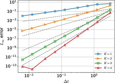
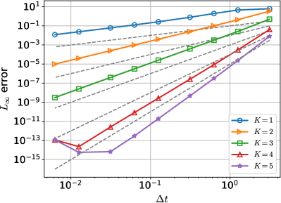
Figure 2: Convergence of SDC for the Dahlquist test equation with MIN-SR-NS preconditioner using $K=1,\ldots,M$ sweeps per per time step. Dashed lines with slopes one to $K$ are shown as a guide to the eye. Left: $M=4$ Radau-Right nodes, right: $M=5$ Lobatto nodes.

Figure 2 shows convergence against the analytical solution for SDC with the MIN-SR-NS preconditioner with $M=4$ Radau-Right nodes (left) and $M=5$ Lobatto nodes (right) for $K=1,2,\dots,M$ sweeps. The underlying collocation methods are of order 7 and 8 so that the order of SDC is determined by $K$. For Radau-Right nodes, SDC gains one order per sweep for $K=1$ and $K=2$ as expected but the third sweep increases the order by two. The same happens for the Lobatto nodes when going from $K=3$ to $K=4$ sweeps. This unexpected order gain has been observed for other configurations of the MIN-SR-NS preconditioner but we do not yet have a theoretical explanation. Nevertheless, this seems an advantage of MIN-SR-NS that we also observe for more complex problems, see §4.2.

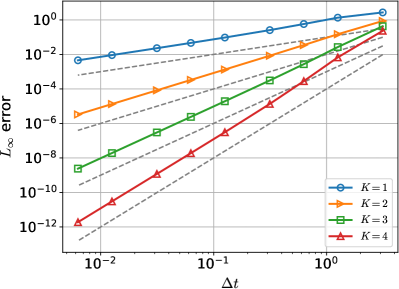
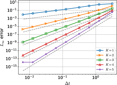
Figure 3: Convergence of SDC for the Dahlquist test equation with MIN-SR-S preconditioner using $K=1,\ldots,M$ sweeps per per time step. Dashed lines with slopes one to $K$ are shown as a guide to the eye. Left: $M=4$ Radau-Right nodes, right: $M=5$ Lobatto nodes.

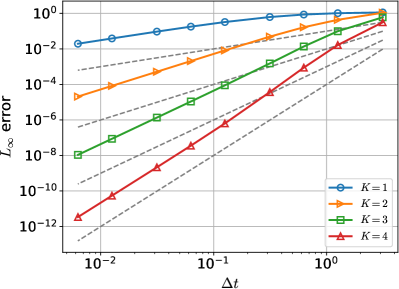
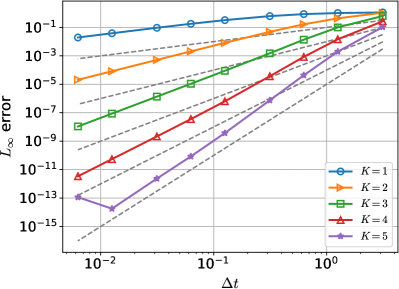
Figure 4: Convergence of SDC for the Dahlquist test equation with MIN-SR-FLEX preconditioner using $K=1,\ldots,M$ sweeps per per time step. Dashed lines with slopes one to $K$ are shown as a guide to the eye. Left: $M=4$ Radau-Right nodes, right: $M=5$ Lobatto nodes.

Figure 3 shows convergence of SDC with MIN-SR-S preconditioner while Figure 4 shows convergence for MIN-SR-FLEX. In both cases the order increases by one per sweep but without the additional gains we oberserved for MIN-SR-NS. Also, errors for MIN-SR-S and MIN-SR-FLEX are generally higher than for MIN-SR-NS. This is expected as MIN-SR-NS is optimized for non-stiff problems and the Dahlquist problem with $\lambda=i$ is not stiff. Note that no results seem to exist in the literature that analyze convergence order for a nonstationary SDC iteration like MIN-SR-FLEX where the preconditioner changes in every iteration.

3.2 Numerical stability

We investigate stability of parallel SDC by numerically computing the borders of its stability region

(50) $$\mathcal{S}_{C}=\left\{z\in\mathbb{C}\;\text{s.t}\;|R(z)|=1\right\},$$

where $R$ is the stability function of a given SDC configuration. We use $M=4$ Radau-Right nodes from a Legendre distribution for all experiments here but other configurations can again be analyzed using the provided code.

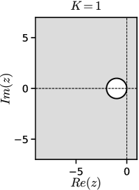
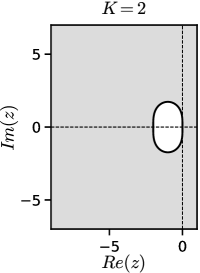
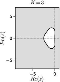
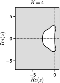
Figure 5: Stability region for SDC with $M=4$ Radau-Right nodes using the PIC preconditioner for $K=1,2,3,4$. The gray zones are unstable areas in the complex plane.

Figure 5. shows stability for SDC with PIC preconditioner (Picard iteration). This is a fully explicit method and, as expected, not $A$-stable for any $K$. Interestingly, $K$-many sweeps reproduce the stability contour of the explicit RKM of order $K$ with $K$ stages. In particular, we recognize the stability contour explicit Euler for $K=1$ and of the classical explicit RKM of order $4$ for $K=4$.

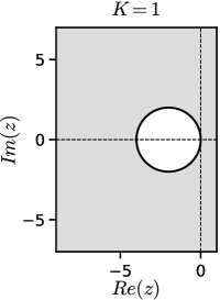
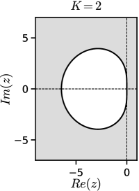
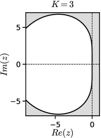
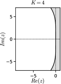
Figure 6: Stability region for SDC with $M=4$ Radau-Right nodes using the MIN-SR-NS preconditioner for $K=1,2,3,4$. The gray zones are unstable areas in the complex plane.

Figure 6 shows stability contours for MIN-SR-NS. As for the Picard iteration, the method is $A$-stable for any number of sweep but the stability regions are significantly larger. That MIN-SR-NS is not $A$-stable is not unexpected since the coefficients are optimized for the non-stiff case where $z\approx 1$.

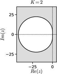
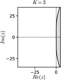
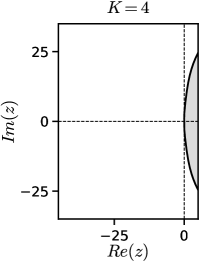
Figure 7: Stability region for SDC with $M=4$ Radau-Right nodes using the MIN-SR-S preconditioner for $K=1,2,3,4$. The gray zones are unstable areas in the complex plane. Note that $\lambda$ ranges are five times larger than for the previous Figures 5 and 6.

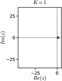
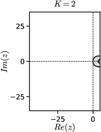
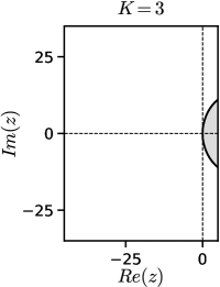
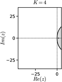
Figure 8: Stability region for SDC with $M=4$ Radau-Right nodes using the MIN-SR-FLEX preconditioner for $K=1,2,3,4$. The gray zones are unstable areas in the complex plane.

Figures 7 and 8 show stability regions for MIN-SR-S and MIN-SR-FLEX. SDC with MIN-SR-S for $K\leq 3$ could be $A$-stable starting while SDC with MIN-SR-FLEX could be $A$-stable for any number of sweeps $K$. However, the apparent $A$-stability holds only for Radau-Right nodes. For example, SDC with $M=5$ Lobatto nodes and $K=4$ sweeps is not $A$-stable (stability contours not shown here). A theoretical investigation of the stability of parallel SDC is left for later work.

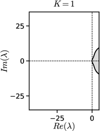
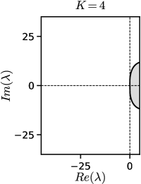
Figure 9: Stability region for SDC with $M=4$ Radau-Right nodes using the LU preconditioner for $K=1,2,3,4$. The gray zones are unstable areas in the complex plane. Note that the stability regions for IE-SDC are very similar.

For comparison, we show the stability contours of the $LU$ preconditioner by Weiser [47] in Figure 9. Stability for SDC with a standard implicit Euler sweeper is very similar and thus not shown. Note that the LU preconditioner is lower triangular and not diagonal and thus does not allow for parallelism in the sweep. Since stability regions of MIN-SR-FLEX and LU are very similar, we can conclude that with an optimized choice of coefficients, parallelism in SDC can be obtained without loss of stability. For further comparison, we show the stability contours for the VDHS preconditioner, obtained by minimizing the spectral radius of $\mathbf{I}-\mathbf{Q}_{\Delta}^{-1}\mathbf{Q}$  [43, Sec. 4.3.4] in Figure 10. For $K=1,2,3$ the stable areas are very small compared to LU or MIN-SR-FLEX and even though the stable regions grows for $K=$, it does not include the imaginary axis, making it unsuitable for oscillatory problems with purely imaginary eigenvalues. Limited numerical stability regions are also observed for the MIN preconditioner [38] (not shown). Since the spectral radius of $\mathbf{I}-\mathbf{Q}_{\Delta}^{-1}\mathbf{Q}$ is significantly larger for MIN than MIN-SR-S and VDHS, we do not consider it in the rest of this paper.

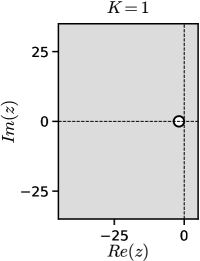
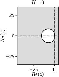
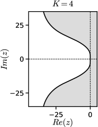
Figure 10: Stability region for SDC with $M=4$ Radau-Right nodes using the VDHS preconditioner for $K=1,2,3,4$. The gray zones are unstable areas in the complex plane.

Remark 3.1.

Experiments not documented here suggest that in approaches based on minimizing the spectral radius of the stiff limit $\mathbf{I}-\mathbf{Q}_{\Delta}^{-1}\mathbf{Q}$, enforcing monotonically increasing coefficients for MIN-SR-S provides a notable improvement in numerical stability.

4 Computational efficiency

We compare computational cost versus accuracy of parallel SDC against SDC preconditioners from the literature and the classical explicit $4^{th}$ order (RK4) and the $L$-stable stiffly accurate implicit RKM ESDIRK4(3)6L[2]SA [20] (ESDIRK43). The two RKM were implemented in pySDC by Baumann et al. [1]. Again all figures in this section can be reproduced using scripts in the provided code [39].

4.1 Estimating computational cost

A fair run-time assessment of parallel SDC requires an optimized parallel implementation which is the subject of a separate work [10]. Here we instead estimate computational cost by considering the elementary operations of each scheme.

To solve a system of ODEs (1), both SDC and RKM need to

1. evaluate the right-hand-side (RHS) $f(u,t)$ for given $u$, $t$ and

2. solve the following non-linear system for some $b$, $t$ and $\alpha$

   (51) $$u-\alpha f(u,t)=b.$$

We solve (51) with an exact Newton iteration, starting from the initial solution $u_{0}$ or the previous SDC iterate $u_{m}^{k-1}$. We stop iterating when a set problem-dependent tolerance is reached or after $300$ iterations. In our numerical experiments, the Jacobian $J_{f}$ can be computed and $I-\alpha J_{f}$ is inverted analytically. In this case, the cost of one Newton iteration is similar to the cost of a RHS evaluation. For RKM, we therefore model that computational cost of a simulation by $N_{\text{Newton}}+N_{\text{RHS}}$. Note that $N_{Newton}=0$ for explicit methods like RK4 or PIC-SDC. For parallel SDC, the computations in every sweep can be parallelized across $M$ threads. However, to account for unavoidable overheads from communication or competition for resources between threads, we assume a parallel efficiency of $P_{\text{eff}}=0.8$ or $80\%$ which should be achievable in an optimized implementation. Thus, we divide the computational cost estimate for SDC by $MP_{\text{eff}}$ instead of $M$.

4.2 Lorenz system

We first consider the non-linear system of ODEs

(52) $$\frac{dx}{dt}=\sigma(y-x),\quad\frac{dy}{dt}=x(\rho-z)-y,\quad\frac{dz}{dt}=xy-\beta z,$$

with $(\sigma,\rho,\beta)=(10,28,8/3)$. The initial value is $(x(0),y(0),z(0))=(5,-5,20)$ and we use a Newton tolerance of $10^{-12}$. We set the final time for the simulation to $T=1.24$, which corresponds to two revolutions around one of the attraction points. A reference solution is computed using an embedded RKM of order 5(4) [6] implemented in scipy with an error tolerance of $10^{-14}$.

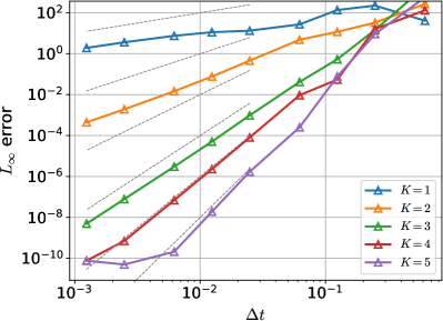
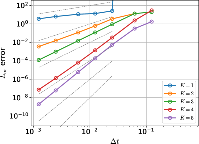
Figure 11: Error vs. time step size for SDC for the Lorenz problem using $M=4$ Radau-Right nodes, for $K=1,\ldots,5$ sweeps per time step. Left: MIN-SR-NS preconditioner, right: PIC preconditioner. Dashed gray ines with slopes from 1 to 6 are shown as a guide to the eye.

Figure 11 shows error versus time step size for MIN-SR-NS for SDC for $K=1,\ldots,5$. Since the Lorenz system is non-stiff, we compare against the Picard iteration (PIC) that is known to be efficient for non-stiff problems. We do see the expected order increase by one per iteration as well as the additional order gain for MIN-SR-NS starting at $K=3$ seen already for the Dahlquist problem. For the same number of sweeps, this makes MIN-SR-NS significantly more accurate than Picard iteration or any other SDC method.

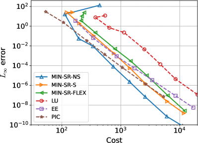
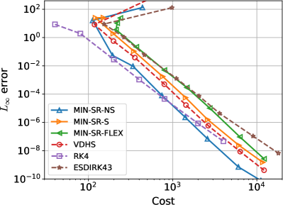
Figure 12: Error vs. cost for SDC for the Lorenz problem using $M=4$ Radau-Right nodes and $K=4$ sweeps. Left: comparison with classical SDC preconditioners, right: comparison with efficient time integration methods from the literature and SDC with VDHS preconditioner.

Figure 12 shows error against computational cost for MIN-SR-S and a variety of other SDC variants (left) as well as RKM and the VDHS preconditioner (right). The parallel and PIC preconditioners significantly outperform classical SDC with explicit Euler or LU sweep. As expected, the preconditioner for non-stiff problems MIN-SR-S is the most efficient although the stiff preconditioners MIN-SR-S and MIN-SR-FLEX remain competitive. MIN-SR-S also outperforms the VDHS preconditioner the ESDIRK43 RKM. For errors above $10^{-4}$, the explicit RKM4 is more efficient than MIN-SR-S but for errors below $10^{-6}$ MIN-SR-S outperforms RKM4. When increasing the number of sweeps to $K=5$, the advantage in efficiency of MIN-SR-S over RKM4 becomes more pronounced, see Figure 13.

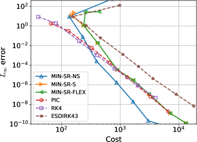
Figure 13: Error vs. cost for SDC and Picard iteration for the Lorenz problem using $M=4$ Radau-Right nodes and $K=5$ sweeps in comparison to RKM4 and ESIDRK43.

4.3 Prothero-Robinson problem

Our second test case is the stiff ODE by Prothero and Robinson [32]

(53) $$\frac{du}{dt}=\frac{u-g(t)}{\varepsilon}+\frac{dg}{dt}.$$

The analytical solution for this ODE is $u(t)=g(t)$ and we set $g(t)=\cos(t)$ and $\varepsilon=10^{-3}$. We also set a Newton tolerance of $10^{-12}$.

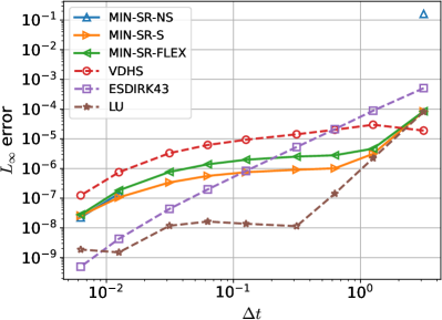
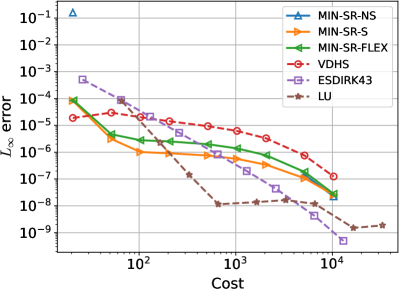
Figure 14: Error vs. time step size for parallel SDC and classical time-integration schemes for the non-linear Prothero-Robinson problem with $\varepsilon=10^{-3}$. SDC uses $M=4$ Radau-Right nodes and $K=4$ sweeps. Left: error vs. time step, right: error vs. cost.

Figure 14 shows error versus time step size (left) and computational cost (right) for our three parallel SDC methods, non-parallel LU-SDC, parallel VDHS SDC and the implicit ESDIRK43 RKM [20]. All SDC variants use $K=4$ sweeps. The parallel SDC variants all show a noticable range of stalling error where the error does not decrease with time step size. This is a known phenomenon for the Prothero-Robinson problem [47, Sec. 6.1] and means that a very small time step is required to recover the theoretically expected convergence order. While MIN-SR-S outperforms LU-SDC in efficiency up to an error of around $10^{-6}$, its stalling convergence after results in LU-SDC being more efficient for very high accuracies.

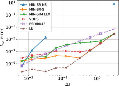
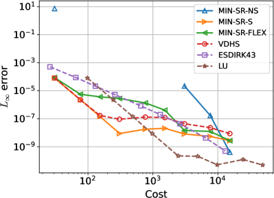
Figure 15: Comparison of diagonal SDC and classical time-integration schemes on the non-linear Prothero-Robinson problem, using $\varepsilon=10^{-3}$. Each SDC configuration uses $M=4$ Radau-Right nodes and $K=6$ sweeps. Left : error vs. time step, right: error vs. cost.

If we increase the number of sweeps to $K=6$, the error level at which convergence stalls is reduced, see Figure 15. This also pushes down the error where LU-SDC becomes more efficient than MIN-SR-S to around $10^{-8}$. Nevertheless, in both cases MIN-SR-S will be an attractive integrator unless extremely tight accuracy is required.

4.4 Allen-Cahn equation

As last test problem, we consider the one-dimensional Allen-Cahn equation with driving force

(54) $$\frac{\partial u}{\partial t}=\frac{\partial^{2}u}{\partial x^{2}}-\frac{2}{\varepsilon^{2}}u(1-u)(1-2u)-6d_{w}u(1-u),\quad x\in[-0.5,0.5],\quad t\in[0,T].$$

using inhomogeneous Dirichlet boundary conditions. The exact solution is

(55) $$u(x,t)=0.5\left[1+\tanh\left(\frac{x-vt}{\sqrt{2}\varepsilon}\right)\right],\quad v=3\sqrt{2}\varepsilon d_{w},$$

and we use it to set the initial solution $u(x,0)$ and the boundary conditions for $x=\pm 0.5$. We set $T=50$ as simulation interval and parameters $\varepsilon=d_{w}=0.04$ The spatial derivative is discretized with a second order finite-difference scheme on $2047$ grid points and we solve (51) in each Newton iteration with a sparse linear solver from scipy. This makes the Newton iteration more expensive than a RHS evaluation so that for this problem we model the cost as $N_{\text{RHS}}+2N_{\text{Newton}}$.

Figure 16 (left) shows the absolute error in the $L_{2}$ norm at $T$ versus the time step size. All methods converge to an error of around $2\cdot 10^{-4}$, which corresponds to the space discretization error for the chosen grid. The fastest converging methods are ESDIRK43 method SDC with LU or MIN-SR-FLEX preconditioners. Because MIN-SR-FLEX can be parallelized, its rapid convergence translates into superior efficiency in Figure 16 (right), showing the absolute $L_{2}$ error versus computational cost. Except for very loose accuracies of $10^{-1}$ and above, MIN-SR-FLEX outperforms the other time-integration methods. Note that for LU to be as efficient as MIN-SR-FLEX for a given time step size, the parallel efficiency of the parallel implementation would need to would need to drop below $40\%$ which would indicate severe performance issues.

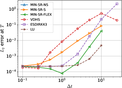
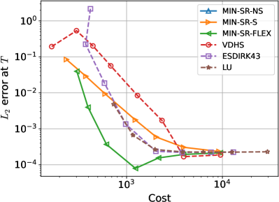
Figure 16: Comparison of diagonal SDC preconditioners and classical time-integration schemes on the Allen-Cahn equation. Each SDC configuration uses $M=4$ Radau-Right nodes and $K=4$ sweeps. Left : error vs. time step, right: error vs. cost.

5 Conclusions

Using a diagonal preconditioner for spectral deferred corrections allows to exploit small-scale parallelization in time for a number of threads up to the number of quadrature nodes in the underlying collocation formula However, efficiency and stability of parallel SDC depends critically on the coefficients in the preconditioner. We consider two minimization problems, one for for stiff and one for non-stiff time-dependent problems, that can be solved to find optimized parameter. This allows us to propose three new sets of coefficients, MIN-SR-NS for non-stiff problems and MIN-SR-S and MIN-SR-FLEX for stiff problems. While we use numerical optimization to determine the MIN-SR-S coefficients, we can obtain the MIN-SR-NS and MIN-SR-FLEX coefficients analytically. MIN-SR-FLEX is a non-stationary iteration where the preconditioner changes in every SDC sweep and is designed to generate a nil-potent error propagation matrix.

We demonstrate by numerical experiments that the three new variants of parallel SDC increase their order by at least one per sweep, similar to existing non-parallel SDC methods. The variants designed for stiff problems have excellent stability properties and might well be $A$-stable, although we do not have a rigorous proof yet. Stability regions of MIN-SR-FLEX in particular are very similar to those of the non-parallel LU-SDC variant and much larger than those of the Iterated Implicit Runge-Kutta methods by Van der Houwen [43]. To assess computational efficiency, we count the number of right hand side evaluations and Newton iterations for all schemes and assume $80\%$ parallel efficiency for the implementation of parallel SDC. We compare error against computational effort for our three new parallel SDC variants, parallel SDC variants from the literature as well as against explicit RKM4 and implicit ESDIRK43 for the non-stiff Lorenz system, the stiff Prothero-Robinson problem and the one-dimensional Allen-Cahn equation, a stiff PDE. For all three test problems, the new parallel SDC variants can outperform previous parallel SDC variants, state-of-the-art serial SDC methods as well as RKM4 and ESDIRK43.

Appendix A Optimized diagonal coefficients for the stiff limit

We repeat here the coefficients used for our numerical experiments, either numerically computed or obtained from the literature as well as the resulting spectral radius of the $\mathbf{K}_{\rm{S}}$ matrix. The values are for $M=4$ Radau-Right nodes from a Legendre distribution.

VDHS by Van der Houwen and Sommeijer [43]

$$\quad\boldsymbol{d}=[0.32049937,\;0.08915379,\;0.18173956,\;0.2333628],\quad\rho(\mathbf{K}_{\rm{S}})=0.025$$

MIN by Speck [38]

$$\quad\boldsymbol{d}=[0.17534868,\;0.0619158,\;0.1381934,\;0.19617814],\quad\rho(\mathbf{K}_{\rm{S}})=0.42$$

MIN3 by Speck et al. [39]

$$\quad\boldsymbol{d}=[0.31987868,\;0.08887606,\;0.18123663,\;0.23273925],\quad\rho(\mathbf{K}_{\rm{S}})=0.0081$$

MIN-SR-S introduced in this paper

$$\quad\boldsymbol{d}=[0.05363588,\;0.18297728,\;0.31493338,\;0.38516736],\quad\rho(\mathbf{K}_{\rm{S}})=0.00024$$

References

- [1] T. Baumann, S. Götschel, T. Lunet, D. Ruprecht, and R. Speck, Adaptive time step selection for spectral deferred corrections, 2024. Submitted.
- [2] K. Burrage, Parallel methods for initial value problems, Applied Numerical Mathematics, 11 (1993), pp. 5–25, https://doi.org/10.1016/0168-9274(93)90037-R.
- [3] J. C. Butcher, On the implementation of implicit Runge–Kutta methods, BIT Numerical Mathematics, 16 (1976), pp. 237–240.
- [4] G. Caklovic, ParaDiag and Collocation Methods: Theory and Implementation, PhD thesis, Karlsruher Institut für Technologie (KIT), 2023, https://doi.org/10.5445/IR/1000164518.
- [5] A. Christlieb, B. Ong, and J.-M. Qiu, Comments on high-order integrators embedded within integral deferred correction methods, Communications in Applied Mathematics and Computational Science, 4 (2009), pp. 27–56, https://doi.org/10.2140/camcos.2009.4.27.
- [6] J. R. Dormand and P. J. Prince, A family of embedded Runge-Kutta formulae, Journal of computational and applied mathematics, 6 (1980), pp. 19–26.
- [7] A. Dutt, L. Greengard, and V. Rokhlin, Spectral Deferred Correction Methods for Ordinary Differential Equations, BIT Numerical Mathematics, 40 (2000), pp. 241–266, https://doi.org/10.1023/A:1022338906936.
- [8] M. Emmett and M. L. Minion, Toward an Efficient Parallel in Time Method for Partial Differential Equations, Communications in Applied Mathematics and Computational Science, 7 (2012), pp. 105–132, https://doi.org/10.2140/camcos.2012.7.105, http://dx.doi.org/10.2140/camcos.2012.7.105.
- [9] R. D. Falgout, S. Friedhoff, T. V. Kolev, S. P. MacLachlan, and J. B. Schroder, Parallel time integration with multigrid, SIAM Journal on Scientific Computing, 36 (2014), pp. C635–C661, https://doi.org/10.1137/130944230, http://dx.doi.org/10.1137/130944230.
- [10] P. Freese, S. Götschel, T. Lunet, D. Ruprecht, and M. Schreiber, Parallel performance of shared memory parallel spectral deferred corrections, 2024. Submitted.
- [11] M. J. Gander, 50 years of Time Parallel Time Integration, in Multiple Shooting and Time Domain Decomposition, Springer, 2015, https://doi.org/10.1007/978-3-319-23321-5_3, http://dx.doi.org/10.1007/978-3-319-23321-5_3.
- [12] C. Gear, Parallel Methods for Ordinary Differential Equations, CALCOLO, 25 (1988), pp. 1–20.
- [13] D. Guibert and D. Tromeur-Dervout, Parallel deferred correction method for CFD problems, in Parallel Computational Fluid Dynamics 2006, Elsevier, 2007, pp. 131–138.
- [14] E. Hairer, S. P. Nørsett, and G. Wanner, Solving Ordinary Differential Equations I: Nonstiff problems, Springer-Verlag Berlin Heidelberg, 2nd ed., 1993, https://doi.org/10.1007/978-3-540-78862-1.
- [15] P. J. V. D. Houwen, B. P. Sommeijer, and W. Couzy, Embedded Diagonally Implicit Runge-Kutta Algorithms on Parallel Computers, Mathematics of Computation, 58 (1992), pp. 135–159.
- [16] J. Huang, J. Jia, and M. Minion, Accelerating the convergence of spectral deferred correction methods, Journal of Computational Physics, 214 (2006), pp. 633–656, https://doi.org/10.1016/j.jcp.2005.10.004.
- [17] A. Iserles and S. P. Nørsett, On the theory of parallel Runge-Kutta methods, IMA Journal of Numerical Analysis, 10 (1990), pp. 463–488, https://doi.org/10.1093/imanum/10.4.463.
- [18] K. R. Jackson, A survey of parallel numerical methods for initial value problems for ordinary differential equations, IEEE Transactions on Magnetics, 27 (1991), pp. 3792–3797, https://doi.org/10.1109/20.104928.
- [19] K. R. Jackson and S. P. Nørsett, The Potential for Parallelism in Runge–Kutta Methods. Part 1: RK Formulas in Standard Form, SIAM Journal on Numerical Analysis, 32 (1995), pp. 49–82, https://doi.org/10.1137/0732002.
- [20] C. A. Kennedy and M. H. Carpenter, Diagonally implicit Runge-Kutta methods for ordinary differential equations. A review, tech. report, 2016.
- [21] S. Leveque, L. Bergamaschi, A. Martinez, and J. W. Pearson, Fast Iterative Solver for the All-at-Once Runge–Kutta Discretization. 2023.
- [22] I. Lie, Some aspects of parallel Runge-Kutta methods, tech. report, Trondheim TU. Inst. Math., Trondheim, 1987, https://cds.cern.ch/record/201368.
- [23] J.-L. Lions, Y. Maday, and G. Turinici, A ”parareal” in time discretization of PDE’s, Comptes Rendus de l’Académie des Sciences - Series I - Mathematics, 332 (2001), pp. 661–668, https://doi.org/10.1016/S0764-4442(00)01793-6, http://dx.doi.org/10.1016/S0764-4442(00)01793-6.
- [24] P. Munch, I. Dravins, M. Kronbichler, and M. Neytcheva, Stage-Parallel Fully Implicit Runge–Kutta Implementations with Optimal Multilevel Preconditioners at the Scaling Limit, SIAM Journal on Scientific Computing, (2023), pp. S71–S96, https://doi.org/10.1137/22m1503270.
- [25] J. Nievergelt, Parallel methods for integrating ordinary differential equations, Communications of the ACM, 7 (1964), pp. 731–733.
- [26] S. P. Nørsett and H. H. Simonsen, Aspects of parallel Runge-Kutta methods, in Numerical Methods for Ordinary Differential Equations, A. Bellen, C. W. Gear, and E. Russo, eds., Berlin, Heidelberg, 1989, Springer Berlin Heidelberg, pp. 103–117.
- [27] B. W. Ong, R. D. Haynes, and K. Ladd, Algorithm 965: RIDC Methods: A Family of Parallel Time Integrators, ACM Trans. Math. Softw., 43 (2016), pp. 8:1–8:13, https://doi.org/10.1145/2964377, http://dx.doi.org/10.1145/2964377.
- [28] B. W. Ong and R. J. Spiteri, Deferred Correction Methods for Ordinary Differential Equations, Journal of Scientific Computing, 83 (2020), https://doi.org/10.1007/s10915-020-01235-8.
- [29] B. Orel, Parallel Runge–Kutta methods with real eigenvalues, Applied Numerical Mathematics, 11 (1993), pp. 241–250, https://doi.org/https://doi.org/10.1016/0168-9274(93)90051-R.
- [30] W. Pazner and P.-O. Persson, Stage-parallel fully implicit Runge–Kutta solvers for discontinuous Galerkin fluid simulations, Journal of Computational Physics, 335 (2017), pp. 700–717, https://doi.org/10.1016/j.jcp.2017.01.050.
- [31] D. Petcu, Experiments with an ODE solver on a multiprocessor system, Computers & Mathematics with Applications, 42 (2001), pp. 1189–1199.
- [32] A. Prothero and A. Robinson, On the stability and accuracy of one-step methods for solving stiff systems of ordinary differential equations, Mathematics of Computation, 28 (1974), pp. 145–162.
- [33] T. Rauber and G. Rünger, Parallel Implementations of Iterated Runge-Kutta Methods, The International Journal of Supercomputer Applications and High Performance Computing, 10 (1996), pp. 62–90, https://doi.org/10.1177/109434209601000103.
- [34] D. Ruprecht and R. Speck, Spectral deferred corrections with fast-wave slow-wave splitting, SIAM Journal on Scientific Computing, 38 (2016), pp. A2535–A2557.
- [35] R. Schöbel and R. Speck, PFASST-ER: combining the parallel full approximation scheme in space and time with parallelization across the method, Computing and Visualization in Science, 23 (2020), https://doi.org/10.1007/s00791-020-00330-5, https://doi.org/10.1007/s00791-020-00330-5.
- [36] S. I. Solodushkin and I. F. Iumanova, Parallel numerical methods for ordinary differential equations: a survey, in CEUR Workshop Proceedings, vol. 1729, CEUR-WS, 2016, pp. 1–10.
- [37] B. Sommeijer, Parallel-iterated Runge-Kutta methods for stiff ordinary differential equations, Journal of Computational and Applied Mathematics, 45 (1993), pp. 151–168, https://doi.org/10.1016/0377-0427(93)90271-C.
- [38] R. Speck, Parallelizing spectral deferred corrections across the method, Comput. Visual Sci., 19 (2018), pp. 75–83, https://doi.org/https://doi.org/10.1007/s00791-018-0298-x.
- [39] R. Speck, T. Lunet, T. Baumann, L. Wimmer, and I. Akramov, Parallel-in-time/pysdc, Mar. 2024, https://doi.org/10.5281/zenodo.10886512, https://doi.org/10.5281/zenodo.10886512.
- [40] P. van der Houwen and B. Sommeijer, Analysis of parallel diagonally implicit iteration of Runge-Kutta methods, Applied Numerical Mathematics, 11 (1993), pp. 169–188, https://doi.org/10.1016/0168-9274(93)90047-U.
- [41] P. van der Houwen, B. Sommeijer, and W. van der Veen, Parallel iteration across the steps of high-order Runge-Kutta methods for nonstiff initial value problems, Journal of Computational and Applied Mathematics, 60 (1995), pp. 309–329, https://doi.org/https://doi.org/10.1016/0377-0427(94)00047-5.
- [42] P. J. Van Der Houwen and B. P. Sommeijer, Parallel iteration of high-order Runge-Kutta methods with stepsize control, Journal of Computational and Applied Mathematics, 29 (1990), pp. 111–127, https://doi.org/10.1016/0377-0427(90)90200-J.
- [43] P. J. van der Houwen and B. P. Sommeijer, Iterated Runge–Kutta Methods on Parallel Computers, SIAM Journal on Scientific and Statistical Computing, 12 (1991), pp. 1000–1028, https://doi.org/10.1137/0912054.
- [44] P. J. Van der Houwen and B. P. Sommeijer, Analysis of parallel diagonally implicit iteration of Runge–Kutta methods, Applied Numerical Mathematics, 11 (1993), pp. 169–188.
- [45] P. J. van der Houwen, B. P. Sommeijer, and W. Van der Veen, Parallelism across the steps in iterated Runge-Kutta methods for stiff initial value problems, Numerical Algorithms, 8 (1994), pp. 293–312.
- [46] W. van der Veen, J. de Swart, and P. van der Houwen, Convergence aspects of step-parallel iteration of Runge-Kutta methods, Applied Numerical Mathematics, 18 (1995), pp. 397–411.
- [47] M. Weiser, Faster SDC convergence on non-equidistant grids by DIRK sweeps, BIT Numerical Mathematics, 55 (2015), pp. 1219–1241, https://doi.org/10.1007/s10543-014-0540-y.