Optimal Control Synthesis of Markov Decision Processes
for Efficiency with Surveillance Tasks

Abstract

We investigate the problem of optimal control synthesis for Markov Decision Processes (MDPs), addressing both qualitative and quantitative objectives. Specifically, we require the system to fulfill a qualitative surveillance task in the sense that a specific region of interest can be visited infinitely often with probability one. Furthermore, to quantify the performance of the system, we consider the concept of efficiency, which is defined as the ratio between rewards and costs. This measure is more general than the standard long-run average reward metric as it aims to maximize the reward obtained per unit cost. Our objective is to synthesize a control policy that ensures the surveillance task while maximizes the efficiency. We provide an effective approach to synthesize a stationary control policy achieving $\epsilon$-optimality by integrating state classifications of MDPs and perturbation analysis in a novel manner. Our results generalize existing works on efficiency-optimal control synthesis for MDP by incorporating qualitative surveillance tasks. A robot motion planning case study is provided to illustrate the proposed algorithm.

I Introduction

Decision-making in dynamic environments is a fundamental challenge for autonomous systems, requiring them to react to uncertainties in real-time to achieve desired tasks with performance guarantees. Markov Decision Processes (MDPs) offer a theoretical framework for sequential decision-making by abstracting uncertainties in both environments and system executions as transition probabilities. Leveraging MDPs allows for the analysis of system behavior and the synthesis of optimal control policies through systematic procedures. In the context of autonomous systems, MDPs have found extensive applications across various domains such as swarm robotics [1], autonomous driving [2], and underwater vehicles [3]; reader is referred to recent surveys for additional references and applications [4, 5].

To assess the performance of infinite horizon behaviors, two widely recognized measures are the long-run average reward (or mean payoff) and the discounted reward [6]. The long-run average reward quantifies the average reward received per state as the system evolves infinitely towards a steady state. However, this measure overlooks the costs incurred for each reward. For instance, a cleaning robot may prioritize collecting more trash while conserving energy. Therefore, recently, the notion of efficiency has emerged to capture the reward-to-cost ratio [7, 8]. Specifically, the efficiency of a system trajectory is defined as the ratio between accumulated reward and accumulated cost. The efficient controller synthesis problem thus aims to maximize the expected long-run efficiency [8].

In addition to maximizing quantitative performance measures, many applications also require achieving qualitative tasks. Recently, within the context of MDPs, there has been a growing interest in synthesizing control policies to maximize the probability of satisfying high-level logic tasks expressed in, for example, linear temporal logic or omega-regular languages. For example, when the MDPs model is known precisely, offline algorithms have been proposed to synthesize optimal controller under LTL specifications; see, e.g., [9, 10, 11, 12]. Recently, reinforcement learning for LTL tasks has also been investigated for MDPs with unknown transition probabilities [13, 14, 15]. One important qualitative task that has been extensively studied is the surveillance task, motivated primarily by persistent surveillance needs in autonomous systems [16, 17, 18]. The surveillance task is essentially equivalent to the concept of Büchi accepting condition requiring that certain desired target states can be visited infinitely often.

In this work, we investigate control policy synthesis for MDPs with both qualitative and quantitative requirements. Specifically, for the qualitative aspect, we require that the surveillance task is satisfied with probability one (w.p.1). Additionally, for the quantitative aspect, we adopt the efficiency measure. Our overarching objective is to maximize the expected long-run efficiency while ensuring the satisfaction of the surveillance task w.p.1. It is worth noting that existing works typically focus on either efficiency optimization (ratio objectives) without qualitative requirements [8], or they consider qualitative requirements but under the standard long-run average reward (mean payoff) measure [19]. In [9], the authors consider qualitative requirement expressed by LTL formulae, with a quantitative measure referred to as the per cycle average reward. However, the per cycle average reward is essentially a special instance of the ratio objective by setting unit cost for specific state on the denominator. To the best of our knowledge, the simultaneous maximization of efficiency while achieving the surveillance task has not been addressed in the existing literature.

To fill this gap in research, we present an effective approach to synthesize stationary policies achieving $\epsilon$-optimality. Our approach integrates state classifications of MDPs [20] and perturbation analysis techniques [21, 22, 23] in a novel manner. Specifically, the key idea of our approach is as follows. Initially, we decompose the MDPs into accepting maximal end components (AMECs) using state classifications, where for each AMEC, we solve the standard efficiency optimization problem without considering the surveillance task [8]. Subsequently, we synthesize a basic policy that achieves optimal efficiency but may fail to fulfill the surveillance task. Finally, we perturb the basic policy “slightly” by a target seeking policy such that the quantitative performance is decreased to $\epsilon$-optimal but the surveillance task is fulfilled. Our approach suggests that perturbation analysis is a conceptually simple yet powerful technique for solving MDPs with both qualitative and quantitative tasks, which may offer new insights into addressing this class of problems. Furthermore, our results also generalized the existing result on perturbation analysis from the long-run average reward optimizations to the case of long-run efficiency optimizations.

The rest of the paper is organized as follows. In Section II, we present some necessary backgrounds and notation. Then we formulate the efficiency optimization problem under surveillance tasks in Section III. In Section IV, we solve the problem for the special case of communicating MDPs based on a new result of perturbation analysis. Then the general case of non-communicating MDPs is tackled in Section V. A case study of robot task planning is provided in Section VI. Finally, we conclude the paper in Section VII.

II Preliminary

II-A Markov Decision Processes

A (finite) Markov decision process (MDP) is a $4$-tuple $\mathcal{M}=(S,s_{0},A,P)$, where $S$ is a finite set of states, $s_{0}\in S$ is the initial state, $A$ is a finite set of actions, and $P:S\times A\times S\rightarrow[0,1]$ is a transition function such that $\forall s\in S,a\in A:\sum_{s^{\prime}\in S}P(s^{\prime}\mid s,a)\in\{0,1\}$. We also write $P(s^{\prime}\mid s,a)$ as $P_{s,a,s^{\prime}}$. For each state $s\in S$, we define $A(s)=\{a\in A:\sum_{s^{\prime}\in S}P(s^{\prime}\mid s,a)=1\}$ as the set of available actions at $s$. We assume that each state has at least one available action, i.e., $\forall s\in S:A(s)\neq\emptyset$. An MDP also induces an underlying directed graph (digraph), where each vertex is a state and an edge of form $\langle s,s^{\prime}\rangle$ is defined if $P(s^{\prime}\mid s,a)>0$ for some $a\in A(s)$.

A Markov chain (MC) $\mathcal{C}$ is an MDP such that $|A(s)|=1$ for all $s\in S$. The transition matrix of MC is denoted by a $|S|\times|S|$ matrix $\mathbb{P}$, i.e., $\mathbb{P}_{s,s^{\prime}}=P(s^{\prime}\mid s,a)$, where $a\in A(s)$ is the unique action at state $s$. Therefore, we can omit actions in MC and write it as $\mathcal{C}=(S,s_{0},\mathbb{P})$. The limit transition matrix of MC is defined by $\mathbb{P}^{\star}=\lim_{n\rightarrow\infty}\frac{1}{n}\sum_{k=0}^{n}\mathbb{P}^{k}$, which always exists for finite MC [6]. Let $\pi_{0}\in\mathbb{R}^{|S|}$ be initial distribution with $\pi_{0}(s)=1$ if $s$ is initial state and $\pi_{0}(s)=0$ otherwise. Then the limit distribution of MC is $\pi=\pi_{0}\mathbb{P}^{\star}$. A state is said to be transient if its corresponding column in the limit transition matrix is a zero vector; otherwise, the state is recurrent.

A policy for an MDP $\mathcal{M}$ is a sequence $\mu=(\mu_{0},\mu_{1},...)$, where $\mu_{k}:S\times A\rightarrow[0,1]$ is a function such that $\forall s\in S:\sum_{a\in A(s)}\mu_{k}(s,a)=1$. A policy is said to be stationary if $\mu_{i}=\mu_{j},\forall i,j$ and we write a stationary policy as $\mu=(\mu,\mu,\dots)$ for simplicity. Given an MDP $\mathcal{M}$, the sets of all policies and all stationary policies are denoted by $\Pi_{\mathcal{M}}$ and $\Pi^{S}_{\mathcal{M}}$, respectively. For policy $\mu\in\Pi_{\mathcal{M}}$, at each instant $k$, it induces a transition matrix $\mathbb{P}^{\mu_{k}}$, where $\mathbb{P}^{\mu_{k}}_{i,j}=\sum_{a\in A(i)}\mu_{k}(i,a)P_{i,a,j}$. A stationary policy $\mu\in\Pi^{S}_{\mathcal{M}}$ induces a time-homogeneous MC with transition matrix $\mathbb{P}^{\mu}$.

An infinite sequence $\rho=s_{0}s_{1}\cdots$ of states is said to be a path in MDP $\mathcal{M}$ under policy $\mu\in\Pi_{\mathcal{M}}$ if $s_{0}$ is initial state of $\mathcal{M}$ and $\forall k\geq 0:\sum_{a\in A(s_{k})}\mu_{k}(s_{k},a)P(s_{k+1}\mid s_{k},a)>0$. We denote by $\textsf{Path}^{\mu}(\mathcal{M})\subseteq S^{\omega}$ the set of all paths in $\mathcal{M}$ under $\mu$, where $S^{\omega}$ denotes the set of all infinite sequences of states. We use the standard probability measure $\textsf{Pr}^{\mu}_{\mathcal{M}}:2^{S^{\omega}}\to[0,1]$ for infinite paths, which satisfies: for any finite sequence $s_{0}\cdots s_{n}$, we have

$$\textsf{Pr}^{\mu}_{\mathcal{M}}(\textsf{Cly}(s_{0}\dots s_{n}))\!=\!\pi_{0}(s_{0})\!\prod_{k=0}^{n-1}\!\sum_{a\in A(s_{k})}\!\!\mu_{k}(s_{k},a)P_{s_{k},a,s_{k+1}},$$

where $\textsf{Cly}(s_{0}\dots s_{n})\subseteq\textsf{Path}^{\mu}(\mathcal{M})$ is set of all paths having prefix $s_{0}\dots s_{n}$ and $\pi_{0}(s)=1$ if $s$ is the initial state and $\pi_{0}(s)=0$ otherwise. The reader is referred to [20] for details on this standard probability measure on infinite paths.

For MDP $\mathcal{M}=(S,s_{0},A,P)$, a sub-MDP is a tuple $(\mathcal{S},\mathcal{A})$, where $\mathcal{S}\subseteq S$ is a non-empty subset of states and $\mathcal{A}:\mathcal{S}\rightarrow 2^{A}\setminus\emptyset$ is a function such that (i) $\forall s\in\mathcal{S}:\mathcal{A}(s)\subseteq A(s)$; and (ii) $\forall s\in\mathcal{S},a\in\mathcal{A}(s):\sum_{s^{\prime}\in\mathcal{S}}P_{s,a,s^{\prime}}=1$. Essentially, $(\mathcal{S},\mathcal{A})$ induces a new MDP by restricting the state space to $\mathcal{S}$ and available actions to $\mathcal{A}(s)$ for each state $s\in\mathcal{S}$.

II-B Ratio Objectives for Efficiency

In the context of MDPs, quantitative measures such as average rewards have been widely used for systems operating in infinite horizons. In [7, 8], a general quantitative measure called ratio objective is proposed to characterize the efficiency of policies. Specifically, two different functions are involved:

• a reward function $\mathtt{R}:S\times A\to\mathbb{R}_{\geq 0}$ assigning each state-action pair a non-negative reward; and

• a cost function $\mathtt{C}:S\times A\to\mathbb{R}_{+}$ assigning each state-action pair a positive cost.

Then the efficiency value from initial state $s_{0}$ under policy $\mu\in\Pi_{\mathcal{M}}$ w.r.t. reward-cost pair $(\mathtt{R},\mathtt{C})$ is defined by

$$J^{\mu}(s_{0},\mathtt{R},\mathtt{C}):=\limsup_{N\to+\infty}E\left\{\frac{\sum_{i=0}^{N}\mathtt{R}(s_{i},a_{i})}{\sum_{i=0}^{N}\mathtt{C}(s_{i},a_{i})}\right\},$$

where $E\left\{\cdot\right\}$ is the expectation of probability measure $\textsf{Pr}_{\mathcal{M}}^{\mu}$. We omit the reward and cost functions if they are clear by context. Intuitively, $J^{\mu}(s_{0})$ captures the average reward the system received per cost, i.e., the efficiency. Let $\Pi\subseteq\Pi_{\mathcal{M}}$ be a set of policies. Then optimal efficiency value among policy set $\Pi$ is denoted by $J(s_{0},\Pi)=\sup_{\mu\in\Pi}J^{\mu}(s_{0})$.

Note that the standard long-run average reward is a special case of ratio objective by taking $\mathtt{C}(s,a)=1,\forall s\in S,a\in A(s)$. For this case, we denote by $W^{\mu}(s_{0},\mathtt{R}):=J^{\mu}(s_{0},\mathtt{R},\mathbf{1})$ the standard long-run average reward from initial state $s_{0}$ under policy $\mu$, and denote by $W(s_{0},\Pi)=\sup_{\mu\in\Pi}W^{\mu}(s_{0})$ the optimal long-run average reward among policy set $\Pi$ .

III Problem Formulation

Note that efficiency does not take qualitative requirements into account, i.e., the system may maximize its efficiency by doing useless things. In this work, motivated by surveillance tasks in autonomous robots, in addition to the ratio objectives, we further consider the qualitative requirement by visiting target states infinitely often.

Formally, let $B\subseteq S$ be a set of target states that need to be visited infinitely. Then the probability of visiting $B$ infinitely often under policy $\mu\in\Pi_{\mathcal{M}}$ is defined by

$$\textsf{Pr}^{\mu}_{\mathcal{M}}(\Box\Diamond B)=\textsf{Pr}^{\mu}_{\mathcal{M}}(\{\tau\in\textsf{Path}^{\mu}(\mathcal{M})\mid\texttt{inf}(\tau)\cap B\neq\emptyset\}),$$

where $\texttt{inf}(\tau)$ denotes the set of states that occur infinite number of times in path $\tau\in\textsf{Path}^{\mu}(\mathcal{M})$. We denote by $\Pi^{B}_{\mathcal{M}}$ the set of all policies under which $B$ is visited infinitely often w.p.1, i.e.,

$$\Pi^{B}_{\mathcal{M}}:=\{\mu\in\Pi_{\mathcal{M}}\mid\textsf{Pr}^{\mu}_{\mathcal{M}}(\Box\Diamond B)=1\}.$$

For the sake of simplicity and without loss of generality, we assume that, starting from any state, there exists a policy such that the surveillance task can be satisfied.

Now we formulate the problem solved in this paper.

Problem 1

Given MDP $\mathcal{M}=(S,s_{0},A,P)$, reward function $\mathtt{R}$, cost function $\mathtt{C}$ and a threshold value $\epsilon>0$, find a stationary policy $\mu^{\star}\in\Pi^{B}_{\mathcal{M}}\cap\Pi_{\mathcal{M}}^{S}$ such that

$$J^{\mu^{\star}}(s_{0})\geq J(s_{0},\Pi^{B}_{\mathcal{M}})-\epsilon.$$ (1)

Remark 1

Before proceeding further, we make several comments on the above problem formulation.

• First, here we seek to find an $\epsilon$-optimal policy $\mu^{\star}$ among all policies satisfying surveillance tasks. The main motivation for this setting is that policies with finite memory are not sufficient to achieve the optimal efficiency value $J(s_{0},\Pi^{B}_{\mathcal{M}})$. Furthermore, even if one employs an infinite memory policy to achieve the optimal efficiency value, the system will visit target states less and less frequently as time progresses. One is referred to [19] regarding this issue for the case of standard long-run average measure, which is a special case of our ratio objective.

• Second, we further restrict our attention to stationary policies in $\Pi_{\mathcal{M}}^{S}$ a priori. We will show in the following result that such a restriction is without loss of generality in the sense that a stationary solution always exists.

Proposition 1

Given MDP $\mathcal{M}=(S,s_{0},A,P)$ and threshold value $\epsilon>0$, there always exists a policy $\mu\in\Pi^{B}_{\mathcal{M}}\cap\Pi^{S}_{\mathcal{M}}$ such that $J^{\mu}(s_{0})\geq J(s_{0},\Pi^{B}_{\mathcal{M}})-\epsilon$.

Proof:

Due to space constraint, the proof is provided in [24]. Note that, the proof here is only existential and one still needs constructive algorithm to effectively synthesize a solution. ∎

IV Case of Communicating MDPs

Before tackling the general case, in this section, we consider a special scenario, where the MDP is communicating. Formally, an MDP $\mathcal{M}$ is said to be communicating if

$$\forall s,s^{\prime}\in S,\exists\mu\in\Pi_{\mathcal{M}},\exists n\geq 0:(\mathbb{P}^{\mu})^{n}_{s,s^{\prime}}>0.$$ (2)

In other words, for a communicating MDP, one state is always able to reach another state.

General Idea: We solve Problem 1 for the case of communicating MDP by the following three steps:

• First, we apply the standard algorithm in [8] to optimize the ratio objective without considering the surveillance task. The resulting policy is denoted by $\mu_{opt}$.

• Second, we select an arbitrary policy $\mu_{sur}$ such that its induced MC is irreducible. Therefore, target states can be visited infinitely often under $\mu_{sur}$.

• Finally, we perturb policy $\mu_{opt}$ “slightly” by $\mu_{sur}$ such that the efficiency value of the resulting policy is $\epsilon$-close to that of $\mu_{opt}$, and the surveillance task can still be achieved due to the presence of perturbation $\mu_{sur}$ .

Now, we proceed the above idea in more detail.

IV-A Efficiency Optimization for Communicating MDP

In this subsection, we review the existing solution for efficiency optimization. It has been shown in [8] that, for communicating MDP $\mathcal{M}$, there exists a stationary policy $\mu\in\Pi^{S}_{\mathcal{M}}$ such that $J^{\mu}(s_{0})=J(s_{0},\Pi_{\mathcal{M}})$ and the induced MC $\mathcal{M}^{\mu}$ is an unichain (MC with a single recurrent class and some transient states). Furthermore, we have

$$J^{\mu}(s_{0})=\frac{\sum_{s\in S}\sum_{a\in A(s)}\pi(s)\mu(s,a)\mathtt{R}(s,a)}{\sum_{s\in S}\sum_{a\in A(s)}\pi(s)\mu(s,a)\mathtt{C}(s,a)},$$ (3)

where $\pi^{\top}\in\mathbb{R}^{|S|}$ is the unique stationary distribution such that $\pi\mathbb{P}^{\mu}=\pi$. With this structural property for communicating MDP, [8] transforms the policy synthesis problem for efficiency optimization to a steady-state parameter synthesis problem described by the nonlinear program (4)-(9) shown as follows:

$$\max_{\gamma(s,a)}\quad\frac{\sum_{s\in S}\sum_{a\in A(s)}\gamma(s,a)\mathtt{R}(s,a)}{\sum_{s\in S}\sum_{a\in A(s)}\gamma(s,a)\mathtt{C}(s,a)}$$ (4)

s.t. $$q(s,t)=\sum_{a\in A(s)}\gamma(s,a)P(t\mid s,a),\forall s,t\in S$$ (5)

$$\lambda(s)=\sum_{a\in A(s)}\gamma(s,a),\forall s\in S$$ (6)

$$\lambda(t)=\sum_{s\in S}q(s,t),\forall t\in S$$ (7)

$$\sum_{s\in S}\lambda(s)=1$$ (8)

$$\gamma(s,a)\geq 0,\forall s\in S,\forall a\in A(s)$$ (9)

Since we will only leverage this existing result, the reader is referred to [8] for more details on the intuition of the above nonlinear program. The only point we would like to emphasize is that this nonlinear program is a linear-fractional programming, which can be solved efficiently by converting to a linear program by Charnes-Cooper transformation [25]. Now, let $\gamma^{\star}(s,a)$ be the solution to Equations (4)-(9). The optimal policy, denoted by $\mu_{opt}$, can be decoded as follows. Let $Q=\{s\in S\mid\sum_{a\in A(s)}\gamma^{\star}(s,a)>0\}$. Then for states in $Q$, we define

$$\mu_{opt}(s,a)=\frac{\gamma^{\star}(s,a)}{\sum_{a\in A(s)}\gamma^{\star}(s,a)},\quad s\in Q.$$ (10)

For the remaining part, policy $\mu_{opt}$ only needs to ensure that states in $S\setminus Q$ are transient states in MC $\mathcal{M}^{\mu_{opt}}$; see, e.g., procedure in [6, Page 480]. Then such a policy $\mu_{opt}$ achieves $J^{\mu_{opt}}(s_{0})=J(s_{0},\Pi_{\mathcal{M}})$. Furthermore, it has been shown in [8] that $\mu_{opt}$ can be deterministic, i.e., $\forall s\in S,\exists a\in A(s):\mu_{opt}(s,a)=1$. Hereafter, we assume that the constructed policy $\mu_{opt}$ is deterministic.

IV-B Efficiency Optimization with Surveillance Tasks

Note that, under policy $\mu_{opt}$, only states in $Q$ are recurrent. Therefore, if $Q\cap B=\emptyset$, then the surveillance task fails. As we mentioned at the beginning of this section, our approach is to perturb $\mu_{opt}$ so that (i) its ratio value will not decrease more than $\epsilon$; and (ii) the surveillance task can be achieved.

To this end, let us consider an arbitrary stationary policy $\mu_{sur}\in\Pi^{S}_{\mathcal{M}}$, which is referred to as the surveillance policy, such that $\mathcal{M}^{\mu_{sur}}$ is irreducible. For policy $\mu_{sur}$, we have

• It is well-defined since we already assume that the MDP $\mathcal{M}$ is communicating. For example, one can simply use the uniform policy as $\mu_{sur}$, i.e., each available action is enabled with the same probability at each state;

• The surveillance task can be achieved by $\mu_{sur}$ since all states can be visited infinitely often w.p.1.

Now, we perturb the optimal policy $\mu_{opt}$ by the surveillance policy $\mu_{sur}$ to obtain a new policy as follows

$$\mu_{pert}:=(1-\delta)\mu_{opt}+\delta\mu_{sur},$$ (11)

where $0<\delta<1$ is the perturbation degree and the above notation means that $\mu_{pert}(s,a)=(1-\delta)\mu_{opt}(s,a)+\delta\mu_{sur}(s,a),\forall s\in S,a\in A(s)$. Clearly, this perturbed policy $\mu_{pert}$ has the following two properties:

• First, we have $J^{\mu_{pert}}(s_{0})\leq J^{\mu_{opt}}(s_{0})$ as $\mu_{opt}$ is already the optimal one to achieve the ratio objective. Furthermore, $J^{\mu_{pert}}(s_{0})\to J^{\mu_{opt}}(s_{0})$ as $\delta\to 0$;

• Second, the surveillance task can still be achieved. This is because, under policy $\mu_{pert}$, the system always has non-zero probability to execute surveillance policy $\mu_{sur}$.

Now, it remains to quantify the relationship between perturbation degree $\delta$ and the performance decrease $J^{\mu_{opt}}(s_{0})-J^{\mu_{pert}}(s_{0})$. That is, how small $\delta$ should be in order to ensure $\epsilon$-optimality.

To this end, we adopt the idea of perturbation analysis of MDP, which is originally developed to quantify the difference of long-run average rewards between two policies [21]. First, we introduce some related definitions.

Definition 1 (Utility Vectors & Potential Vectors)

Let $\mu\in\Pi_{\mathcal{M}}^{S}$ be a stationary policy and $\mathtt{V}:S\times A\to\mathbb{R}$ be a generic utility function, which can be either the reward function $\mathtt{R}$ or the cost function $\mathtt{C}$. Then

• the utility vector of policy $\mu$ (w.r.t. utility function $\mathtt{V}$), denoted by $v^{\mu}_{\mathtt{V}}\in\mathbb{R}^{|S|}$, is defined by

  $$v^{\mu}_{\mathtt{V}}(s)=\sum_{a\in A(s)}\mu(s,a)\mathtt{V}(s,a).$$ (12)

• the potential vector of policy $\mu$ (w.r.t. utility function $\mathtt{V}$), denoted by $g^{\mu}_{\mathtt{V}}\in\mathbb{R}^{|S|}$, is defined by

  $$g_{\mathtt{V}}^{\mu}=(I-\mathbb{P}^{\mu}+(\mathbb{P}^{\mu})^{\star})^{-1}v^{\mu}_{\mathtt{V}}.\vskip 6.0pt plus 2.0pt minus 2.0pt\vskip 6.0pt plus 2.0pt minus 2.0pt$$ (13)

In the above definition, the potential vector is well-defined as matrix $I-\mathbb{P}^{\mu}+(\mathbb{P}^{\mu})^{\star}$ is always invertible [6], where $(\mathbb{P}^{\mu})^{\star}$ is the limit transition matrix of $\mathbb{P}^{\mu}$. Intuitively, the potential vector $g^{\mu}_{\mathtt{V}}$ contains the information regarding the long run average utility in MC $\mathcal{M}^{\mu}$. Specifically, let $\pi_{\mu}$ be the limit distribution of MC $\mathcal{M}^{\mu}$. Then we have

$$\pi_{\mu}^{\top}g^{\mu}_{\mathtt{V}}=\pi_{\mu}^{\top}v^{\mu}_{\mathtt{V}}=W^{\mu}(s_{0},\mathtt{V}),$$

which computes the long run average utility under $\mu$.

Next, we define notion of deviation vectors of two different policies.

Definition 2 (Deviation Vectors)

Let $\mu,\mu^{\prime}\in\Pi^{S}_{\mathcal{M}}$ be two stationary policies and $\mathtt{V}:S\times A\to\mathbb{R}$ be a utility function. Then the deviation vector from $\mu$ to $\mu^{\prime}$ (w.r.t. utility function $\mathtt{V}$) is defined by

$$\mathbf{D}_{\mathtt{V}}(\mu,\mu^{\prime})=(v^{\mu^{\prime}}_{\mathtt{V}}-v^{\mu}_{\mathtt{V}})+(\mathbb{P}^{\mu^{\prime}}-\mathbb{P}^{\mu})g_{\mathtt{V}}^{\mu}.\vskip 6.0pt plus 2.0pt minus 2.0pt$$ (14)

The deviation vector can be used to compute the difference between the long-run average utility of the original policy and the perturbed policy. Formally, let $\mu,\mu^{\prime}\in\Pi^{S}_{\mathcal{M}}$ be two stationary policies, $\mathtt{V}:S\times A\to\mathbb{R}$ be a utility function and $\delta\in(0,1)$ be the perturbation degree. We define

$$\mu_{\delta}=(1-\delta)\mu+\delta\mu^{\prime}$$

as the $\delta$-perturbed policy of $\mu$ by $\mu^{\prime}$. It was shown in [21] that, when $\mathcal{M}^{\mu}$ is a unichain, the differences between the long run average utilities of the perturbed policy and the original policy can be calculated as follow:

$$W^{\mu_{\delta}}(s_{0},\mathtt{V})-W^{\mu}(s_{0},\mathtt{V})=\pi_{\mu_{\delta}}^{\top}v_{\mathtt{V}}^{\mu_{\delta}}-\pi_{\mu}^{\top}v_{\mathtt{V}}^{\mu}=\delta\pi_{\mu_{\delta}}^{\top}\textbf{D}_{\mathtt{V}}(\mu,\mu^{\prime}).$$ (15)

However, the above classical result can only be applied to the case of long-run average reward. The following proposition provides the key result of this subsection, which shows how to generalize Equation (15) from long-run average reward to the case of long-run efficiency under the ratio objective.

Proposition 2

Let $\mu,\mu^{\prime}\in\Pi^{S}_{\mathcal{M}}$ be two stationary policies, $\mathtt{R}:S\times A\to\mathbb{R}_{\geq 0}$ be the reward function, $\mathtt{C}:S\times A\to\mathbb{R}_{+}$ be the cost function, and $\delta\in(0,1)$ be the perturbation degree. Let $\mu_{\delta}=(1-\delta)\mu+\delta\mu^{\prime}$ be the perturbed policy. If $\mathcal{M}^{\mu}$ is unichain, then we have

$$J^{\mu_{\delta}}(s_{0},\mathtt{R},\mathtt{C})-J^{\mu}(s_{0},\mathtt{R},\mathtt{C})$$ (16)

$$= \frac{\delta}{\pi_{\mu_{\delta}}^{\top}v_{\mathtt{C}}^{\mu_{\delta}}}\pi_{\mu_{\delta}}^{\top}\left(\textbf{D}_{\mathtt{R}}(\mu,\mu^{\prime})-J^{\mu}(s_{0},\mathtt{R},\mathtt{C})\textbf{D}_{\mathtt{C}}(\mu,\mu^{\prime})\right)\vskip 6.0pt plus 2.0pt minus 2.0pt\vskip 6.0pt plus 2.0pt minus 2.0pt$$

Proof:

First, we note that the perturbed policy $\mu_{\delta}$ induces unichain MC; detailed proofs for this is provided in  [24]. Then we have the following equalities

$$J^{\mu_{\delta}}(s_{0})-J^{\mu}(s_{0})$$

$$= \frac{\pi_{\mu_{\delta}}^{\top}v_{\mathtt{R}}^{\mu_{\delta}}}{\pi_{\mu_{\delta}}^{\top}v_{\mathtt{C}}^{\mu_{\delta}}}-\frac{J^{\mu}(s_{0})\pi_{\mu_{\delta}}^{\top}v_{\mathtt{C}}^{\mu_{\delta}}}{\pi_{\mu_{\delta}}^{\top}v_{\mathtt{C}}^{\mu_{\delta}}}$$

$$= \frac{\pi_{\mu_{\delta}}^{\top}v_{\mathtt{R}}^{\mu_{\delta}}-\pi_{\mu}^{\top}v_{\mathtt{R}}^{\mu}-J^{\mu}(s_{0})(\pi_{\mu_{\delta}}^{\top}v_{\mathtt{C}}^{\mu_{\delta}}-\pi_{\mu}^{\top}v_{\mathtt{C}}^{\mu})}{\pi_{\mu_{\delta}}^{\top}v_{\mathtt{C}}^{\mu_{\delta}}}$$

$$= \frac{\delta}{\pi_{\mu_{\delta}}^{\top}v_{\mathtt{C}}^{\mu_{\delta}}}\pi_{\mu_{\delta}}^{\top}(\textbf{D}_{\mathtt{R}}(\mu,\mu^{\prime})-J^{\mu}(s_{0})\textbf{D}_{\mathtt{C}}(\mu,\mu^{\prime})).$$

Specifically, the first and the second equalities hold because $\mu_{\zeta}$ and $\mu$ induce unichain MCs and the efficiency values can be computed by Equation (3). The last equality comes from Equation (15). This completes the proof. ∎

Remark 2

Clearly, our new result in Equation (16) for ratio objective subsumes the classical result in Equation (15) for the case of long-run average reward. Specifically, when $\mathtt{C}(s,a)=1,\forall s\in S,a\in A(s)$, $J^{\mu}(s_{0},\mathtt{R},\mathtt{C})$ reduces to $W^{\mu}(s_{0},\mathtt{R})$. For this case, we know that $\pi_{\mu_{\delta}}^{\top}v_{\mathtt{C}}^{\mu_{\delta}}=1$ as $v^{\mu}_{\mathtt{C}}(s)=1,\forall s\in S$. Furthermore, we have $\textbf{D}_{\mathtt{C}}(\mu,\mu^{\prime})=0$ as both policies achieve the same cost. Therefore, Equation (16) becomes to Equation (15) and our result provides a more general form of perturbation analysis in terms of deviation vectors.

Now let us discuss how to use Proposition 2 to determine the perturbation degree $\delta$ such that $\epsilon$-optimality holds. Note that, in Equation (16), term $\textbf{D}_{\mathtt{R}}(\mu,\mu^{\prime})-J^{\mu}(s_{0},\mathtt{R},\mathtt{C})\textbf{D}_{\mathtt{C}}(\mu,\mu^{\prime})$ can be computed explicitly based on $\mu$ and $\mu^{\prime}$. However, term $\frac{\pi_{\mu_{\delta}}^{\top}}{\pi_{\mu_{\delta}}^{\top}v_{\mathtt{C}}^{\mu_{\delta}}}$ cannot be directly computed. Our approach here is to estimate its bound as follows:

• Let $c_{min}=\min_{s\in S,a\in A(s)}\mathtt{C}(s,a)$ be minimum cost for all state-action pairs. Then we have $\pi_{\mu_{\delta}}^{\top}v_{\mathtt{C}}^{\mu_{\delta}}\geq c_{min}$.

• Let the infinity norm of the computable part be

  $$\textbf{D}_{\infty}^{\mu,\mu^{\prime}}=\|\textbf{D}_{\mathtt{R}}(\mu,\mu^{\prime})-J^{\mu}(s_{0})\textbf{D}_{\mathtt{C}}(\mu,\mu^{\prime})\|_{\infty}.$$ (17)

  We have $|\pi_{\mu_{\zeta}}^{\top}(\textbf{D}_{\mathtt{R}}(\mu,\mu^{\prime})-J^{\mu}(s_{0})\textbf{D}_{\mathtt{C}}(\mu,\mu^{\prime}))|\leq\textbf{D}_{\infty}^{\mu,\mu^{\prime}}$.

These inequalities lead to the following result.

Proposition 3

Let $\mathcal{M}=(S,s_{0},A,P)$ be a communicating MDP, $\mu_{opt}\in\Pi^{S}_{\mathcal{M}}$ be the optimal policy for ratio objective, $\mu_{sur}\in\Pi^{S}_{\mathcal{M}}\cap\Pi^{B}_{\mathcal{M}}$ be a surveillance policy, and $\mu_{pert}$ be defined in (11). If

$$\delta\leq\epsilon\frac{c_{min}}{\textbf{D}_{\infty}^{\mu_{opt},\mu_{sur}}},$$ (18)

then we have $J^{\mu_{pert}}(s_{0})\geq J^{\mu_{opt}}(s_{0})-\epsilon$.

Proof:

To show this, we have

$$\left|J^{\mu_{pert}}(s_{0})-J^{\mu_{opt}}(s_{0})\right|$$

$$= \frac{\delta\left|\pi_{\mu_{pert}}^{\top}(\textbf{D}_{\mathtt{R}}(\mu_{opt},\mu_{sur})-J^{\mu}(s_{0})\textbf{D}_{\mathtt{C}}(\mu_{opt},\mu_{sur}))\right|}{\pi_{\mu_{pert}}^{\top}v_{\mathtt{C}}^{\mu_{pert}}}$$

$$\leq \frac{\delta}{c_{min}}\left|\pi_{\mu_{pert}}^{\top}(\textbf{D}_{\mathtt{R}}(\mu_{opt},\mu_{sur})-J^{\mu}(s_{0})\textbf{D}_{\mathtt{C}}(\mu_{opt},\mu_{sur}))\right|$$

$$\leq \frac{\delta}{c_{min}}\pi_{\mu_{pert}}^{\top}\mathbf{1}\|\textbf{D}_{\mathtt{R}}(\mu_{opt},\mu_{sur})-J^{\mu}(s_{0})\textbf{D}_{\mathtt{C}}(\mu_{opt},\mu_{sur})\|_{\infty}$$

$$= \frac{\delta}{c_{min}}\textbf{D}_{\infty}^{\mu_{opt},\mu_{sur}}\leq\epsilon$$

where $\mathbf{1}\in\mathbb{R}^{|S|}$ is the vector where all elements are one. Note that, the first equality comes from Proposition 2. Then the first inequality holds since $\pi_{\mu_{pert}}^{\top}v_{\mathtt{C}}^{\mu_{pert}}\geq c_{min}\pi_{\mu_{pert}}^{\top}\mathbf{1}=c_{min}>0$. This completes the proof. ∎

Finally, based on Proposition 3, we can establish the main theorem showing the correctness of our approach.

Theorem 1

Let $\mathcal{M}=(S,s_{0},A,P)$ be a communicating MDP. If $\delta$ satisfies Equation (18), then policy $\mu_{pert}$ defined in (11) is a solution to Problem 1.

Proof:

The proof is provided in [24]. ∎

Remark 3

In our approach, we do not specify how to choose the surveillance policy $\mu_{sur}\in\Pi^{S}_{\mathcal{M}}\cap\Pi^{B}_{\mathcal{M}}$. In practice, however, if the efficiency of surveillance policy $\mu_{sur}$ itself is very small, then $\textbf{D}_{\infty}^{\mu_{opt},\mu_{sur}}$ will be very large. According to Equation (18), it means that we need to select a small perturbation degree $\delta$ to ensure $\epsilon$-optimality. This result is intuitive as we need to employ $\mu_{opt}$ more frequently such that the overall efficiency will not decrease too much. However, this also means that we will visit target states less frequently although they are still guaranteed to be visited infinitely often w.p.1. How to maximize the frequency of visiting target states under the $\epsilon$-optimality constraint is beyond the scope of this paper. A direct heuristic approach is to obtain $\mu_{sur}$ by modifying $\mu_{opt}$ so that their difference in efficiency is “minimized”.

V Solution to the General Case

V-A Overview of Our Approach

The approach in the previous section assumes that MDP $\mathcal{M}$ is communicating. In general, however, the MDP may not be communicating and the optimal ratio objective policy may induce a multi-chain MC, i.e., an MC containing more than one recurrent classes. Our approach for handling the general case consists of the following steps:

1. First, we decompose the MDP into several communicating sub-MDPs containing target states, which are referred to as accepting maximal end components (AMEC). Eventually, the system needs to stay within these AMECs in order to achieve the surveillance task;

2. Next, for each AMEC, since it is communicating, we can compute the optimal efficiency value one can achieve within the AMEC by the nonlinear program (4)-(9) as discussed in Section IV-A;

3. Note that, since we consider long-run objectives, the efficiency value counts only when one decides to stay in some AMEC forever. Therefore, we construct a standard long-run average reward (per-stage) optimization problem, in which the reward for each state is determined by the optimal efficiency value of its associated AMEC (if any). This gives us a basic policy such that it attains the optimal efficiency value within all policies in $\Pi_{\mathcal{M}}^{B}$ (but may has not yet achieve the surveillance task);

4. Finally, for the basic policy, we perturb within each AMEC using the approach in Section IV-B such that the efficiency value decreases to $\epsilon$-optimal but the surveillance task is achieved.

Before presenting our formal algorithm, we further introduce some necessary concepts.

Definition 3 (Accepting Maximal End Components)

A sub-MDP $(\mathcal{S},\mathcal{A})$ of $\mathcal{M}=(S,s_{0},A,P)$ is said to be an end component if its underlying digraph is strongly connected. We say $(\mathcal{S},\mathcal{A})$ is an maximal end component if it is an end component and there is no other end component $(\mathcal{S}^{\prime},\mathcal{A}^{\prime})$ such that (i) $\mathcal{S}\subseteq\mathcal{S}^{\prime}$; and (ii) $\mathcal{A}\subseteq\mathcal{A}^{\prime}$. We denote by $\texttt{MEC}(\mathcal{M})$ the set of all MECs in $\mathcal{M}$. An MEC is said to be an accepting MEC (AMEC) if $\mathcal{S}\cap B\neq\emptyset$; we denote by $\texttt{AMEC}(\mathcal{M})\subseteq\texttt{MEC}(\mathcal{M})$ the set of AMECs.

Now suppose that $\mathcal{M}$ has $n$ AMECs denoted by $\texttt{AMEC}(\mathcal{M})=\{(\mathcal{S}_{1},\mathcal{A}_{1}),\dots,(\mathcal{S}_{n},\mathcal{A}_{n})\}$, which can be computed in polynomial time by Algorithm 47 in [20]. For each AMEC $(\mathcal{S}_{i},\mathcal{A}_{i})$, we denote by $\mu_{opt}^{i}$ and $J^{\mu_{opt}^{i}}$ the optimal policy for ratio objective $(\mathtt{R},\mathtt{C})$ and its corresponding efficiency value computed by program (4)-(9), respectively.

Note that we already assume, without loss of generality that, $\mu_{opt}^{i}$ is deterministic. Let $K\in\mathbb{R}$ be a real number. Then based on $K$ and $\mu_{opt}^{i},i=1,\dots,n$, we define a new reward function $\texttt{R}_{K}:S\times A\to\mathbb{R}$ for the entire $\mathcal{M}$ by:

$$\texttt{R}_{K}(s,a)\!=\!\left\{\!\!\begin{array}[]{cl}J^{\mu_{opt}^{i}}&\text{if }s\in\mathcal{S}_{i}\wedge\mu_{opt}^{i}(s,a)=1\\ K&\text{otherwise}\end{array}\right.\!\!\!.$$ (21)

Intuitively, for each optimal state-action pair in an AMEC, the above construction assigns exactly the same reward identical to the optimal efficiency value one can achieve within this AMEC. For the remaining state-action pairs that are either non-optimal or not in AMECs, we assign them value $K$. Clearly, for the purposes of being optimal or to fulfill the surveillance task, one needs to avoid executing such state-action pair with value $K$. Hence, one needs to select $K$ to be sufficiently small and we will show later in Section V-C how small $K$ can ensure so.

Later on, we also need to solve the classical long-run average reward maximization problem of $\mathcal{M}$ w.r.t. reward function $\texttt{R}_{K}$. We denote by $\mu^{\star}_{K}\in\Pi_{\mathcal{M}}^{S}$ the optimal long-run average reward policy, i.e.,

$$W^{\mu^{\star}_{K}}(s_{0},\texttt{R}_{K})=W(s_{0},\texttt{R}_{K},\Pi_{\mathcal{M}}).$$

Such optimal policy $\mu^{\star}_{K}$ can be obtained by the standard linear programming approach in [6].

Input: MDP $\mathcal{M}=(S,s_{0},A,P)$, target set $B\subseteq S$ and threshold value $\epsilon>0$

Output: Policy $\mu^{\star}\in\Pi^{S}_{\mathcal{M}}$ which solve Problem 1

1

2Compute all AMECs $\texttt{AMEC}(\mathcal{M})$ in $\mathcal{M}$;

3 For each AMEC $(\mathcal{S}_{i},\mathcal{A}_{i})\in\texttt{AMEC}(\mathcal{M})$, compute $\mu_{opt}^{i}$ and $J^{\mu_{opt}^{i}}$ by program (4)-(9) over $(\mathcal{S}_{i},\mathcal{A}_{i})$;

4 Define reward function $\mathtt{R}_{K}$ according to Eq. (21), where $K$ satisfies Eq. (26);

5 Compute policy $\mu_{K}^{\star}$ by solving the classical long-run average reward maximization problem w.r.t. $\mathtt{R}_{K}$;

6 $\mu^{\star}\leftarrow\mu_{K}^{\star}$;

7 for $(\mathcal{S}_{i},\mathcal{A}_{i})\in\texttt{AMEC}(\mathcal{M})$ do

8       if $\mathcal{S}_{i}$ contains a recurrent state in MC $\mathcal{M}^{\mu_{K}^{\star}}$ then

9             Find a surveillance policy $\mu^{i}_{sur}$ for sub-MDP $(\mathcal{S}_{i},\mathcal{A}_{i})$

10             Pick $\delta>0$ satisfying Equation (18)

11             Perturb the policy $\mu^{\star}$ by $\mu^{i}_{sur}$ with degree $\delta$ for the part of sub-MDP $(\mathcal{S}_{i},\mathcal{A}_{i})$, i.e.,

$$\!\!\!\mu^{\star}(s,a)\!\leftarrow\!\!\left\{\begin{array}[]{ll}\!\!(1-\delta)\mu^{\star}(s,a)+\delta\mu_{sur}^{i}(s,a)&\\ &\!\!\!\!\!\!\!\!\!\!\!\!\!\!\!\!\!\!\!\!\!\!\!\!\!\!\!\!\!\!\!\text{if }s\in\mathcal{S}_{i},a\in\mathcal{A}_{i}\\ \mu^{\star}(s,a)&\!\!\!\!\!\!\!\!\!\!\!\!\!\!\!\!\!\!\!\!\!\!\!\!\!\!\!\!\!\!\!\text{otherwise}\end{array}\right.$$ (25)

12      

Return $\epsilon$-optimal policy $\mu^{\star}$

Algorithm 1 Policy Synthesis for the General Case

V-B Main Synthesis Algorithm

Based on the above informal discussions, our overall synthesis procedure for the entire MDP $\mathcal{M}$ is provided in Algorithm 1. Specifically, in line 1, we first compute all AMECs. Then we solve program (4)-(9) for each AMEC and record the constructed policy and optimal efficiency value in lines 2. These policies and values help us to define reward function $\mathtt{R}_{K}$, for which the maximum average reward policy $\mu^{\star}_{K}$ is synthesized. These are done by lines 3-4. Note that $K$ needs to be chosen sufficiently small so that MDP will not stay in those non-AMEC states. Then in line 5, we choose $\mu^{\star}_{K}$ as the initial policy to be perturbed.

Finally, in lines 7-11, based on the initial policy, we determine whether each AMEC $(\mathcal{S}_{i},\mathcal{A}_{i})$ contains some recurrent state in MC $\mathcal{M}^{\mu_{K}^{\star}}$. If so, it means that the MDP will achieve higher efficiency value when choosing to stay in this AMEC forever. Therefore, within this AMEC, we perturb the initial policy by $\mu_{sur}$ slightly to achieve $\epsilon$-optimality and the surveillance task. Note that, since we perturbed each AMEC each containing recurrent states to each $\epsilon$-optimality, the overall perturbed policy $\mu^{\star}$ is still $\epsilon$-optimal.

Remark 4

In fact, for each recurrent class in MC $\mathcal{M}^{\mu_{K}^{\star}}$, we can first check if it already contains a target state in $B$. If so, then we can skip the perturbation procedure in lines 8-11, and the resulting policy within the associated AMEC will actually be optimal rather than $\epsilon$-optimal.

V-C Properties Analysis and Correctness

We conclude this section by formally analyzing the properties of the proposed algorithm.

Still, for $i=1,\dots,n$, we denote by $J^{\mu_{opt}^{i}}$ the optimal efficiency value one can achieve for AMEC $(\mathcal{S}_{i},\mathcal{A}_{i})$ and define

$$J_{max}= \max\{J^{\mu_{opt}^{1}},J^{\mu_{opt}^{2}},\dots,J^{\mu_{opt}^{n}}\}$$

$$J_{min}= \min\{J^{\mu_{opt}^{1}},J^{\mu_{opt}^{2}},\dots,J^{\mu_{opt}^{n}}\}$$

$$p_{min}= \min\{P_{s,a,t}\mid s,t\in S,a\in A(s),P_{s,a,t}>0\}.$$

The following result shows that, by selecting $K$ to be sufficiently small, the solution to the long-run average reward maximization problem w.r.t. reward function $\mathtt{R}_{K}$ indeed achieves the supremum efficiency value among all policies in $\Pi_{\mathcal{M}}^{B}$.

Proposition 4

If $K$ is selected such that

$$K\leq-\frac{1}{p_{min}}(J_{max}-J_{min}),$$ (26)

then we have $W(s_{0},\mathtt{R}_{K},\Pi_{\mathcal{M}})=J(s_{0},\mathtt{R},\mathtt{C},\Pi^{B}_{\mathcal{M}}).$

Proof:

The proof is provided in [24]. ∎

Based on the above criterion, we can finally establish the correctness result of the synthesis procedure for the general case of non-communicating MDPs.

Theorem 2

If $K$ is selected such that Equation (26) holds, then Algorithm 1 correctly solves Problem 1.

Proof:

The proof is provided in [24]. ∎

VI Case Study

In this section, we present a case study of robot task planning to illustrate the proposed method. All computations are performed on a desktop with 16 GB RAM. We use CVXPY [26] to solve convex optimization problems.

Mobility of Robot: We consider a mobile robot moving in a $9\times 9$ gird workspace shown in Figure 1(a). The initial location of the robot is the blue grid in the upper left corner and red girds represent obstacle regions the robot cannot enter. We assume that the mobility of the robot is fully deterministic. That is, at each gird, the robot has at most four actions, left/right/up/down, and the robot can deterministically move to the unique corresponding successor grid by taking each action. An action is not available if it leads to the boundary or the obstacle regions. Therefore, the mobility of the robot can be modeled as a deterministic MDP denoted by $\hat{\mathcal{M}}=(\hat{S},\hat{s}_{0},\hat{P},\hat{A})$ with state space $\hat{S}=\{(i,j):i,j=1,\dots,9\}$.

Probabilistic Environment: The objective of the robot is to find and pick up items in the workspace and then deliver to the one of the destinations in $\hat{B}\subseteq\hat{S}$, which are denoted by green grids. We assume that, at each time instant, when the robot is at grid $\hat{s}\in\hat{S}$, it has probability $p(\hat{s})$ to find an item; the probability distribution over the workspace is shown in Figure 1(b). If the robot is empty, then it will pick up the item immediately when find it and the robot can only carry at most one item.

MDP Model: The overall behavior of both the deterministic mobility and the probabilistic environment can be captured by MDP $\mathcal{M}=({S},{s}_{0},{P},A=\hat{A})$ with augmented state space $S=\hat{S}\times\{0,1\}$, where $0$ means that the robot is empty and $1$ means that it is carrying item. We assume that the robot is initially empty, i.e., $s_{0}=(\hat{s}_{0},0)$. The set of target states in the augmented state space is $B=\hat{B}\times\{1\}$, i.e., when the robot is at the destination with item. Then the transition probability is defined by: for any states $s=(\hat{s},i)$, $s^{\prime}=(\hat{s}^{\prime},i^{\prime})$ and action $a\in A=\hat{A}$, we have

1. if $\hat{P}(\hat{s}^{\prime}\mid\hat{s},a)=0$, then $P(s^{\prime}\mid s,a)=0$;

2. otherwise, we have

$$P(s^{\prime}|s,a)=\left\{\begin{array}[]{ll}p(\hat{s}^{\prime})&\text{if }i=0\wedge i^{\prime}=1\\ 1-p(\hat{s}^{\prime})&\text{if }i=0\wedge i^{\prime}=0\\ 1&\text{if }i=1\wedge i^{\prime}=1\wedge s\notin B\\ p(\hat{s}^{\prime})&\text{if }i=1\wedge i^{\prime}=1\wedge s\in B\\ 1-p(\hat{s}^{\prime})&\text{if }i=1\wedge i^{\prime}=0\wedge s\in B\\ \end{array}\right.$$ (32)

Costs and Rewards: We assume that moving from each grid incurs a cost. Specifically, for each state $s=(\hat{s},i)\in S$ and action $a\in A$, the moving cost $\mathtt{C}(s,a)$ is defined by $\mathtt{C}(s,a)=\textsf{cost}(M(\hat{s}))$, where $M(\hat{s})$ is the shortest Manhattan distance from $\hat{s}$ to target grids and $\textsf{cost}(\cdot)$ is shown in Table I. Also, the robot receives a reward when reaching the destinations. We assume that the rewards for destinations $s_{ll}\in B$ in the lower left and $s_{ur}\in B$ in the upper right corner are different with $\mathtt{R}(s_{ll},a)=2$ and $\mathtt{R}(s_{ur},a)=1$ for all $a\in A$. Then the overall objective of the robot is to visit $B$ infinitely often w.p.1 while maximizing the expected long-run reward-to-cost ratio.

TABLE I: Cost function based on Manhattan distance

Distance	0	1	2	3	4	5	6	7	8
Cost	3.2	3.0	2.7	2.5	1.5	1.0	0.8	0.6	0.5

(a) Workspace of the robot, where arrows indicate optimal actions.

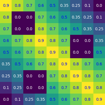
(b) Probabilities for finding items.

Figure 1: Case study of robot planning.

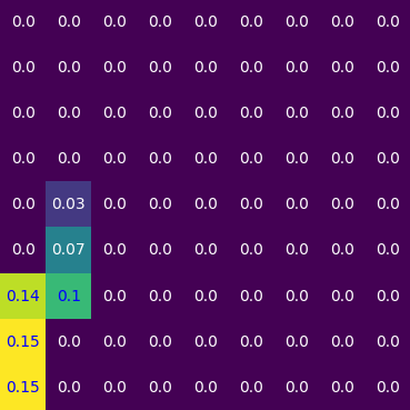
(a) Limit distribution for $\hat{S}\times\{1\}$.

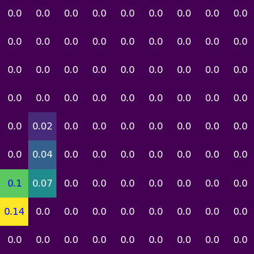
(b) Limit distribution for $\hat{S}\times\{0\}$.

Figure 2: Limit distribution under the optimal policy.

Solution Analysis: By applying the synthesis algorithm, the robot will first take an arbitrary transient path and then eventually circulate along the path shown in Figure 1(a). Specifically, the red and blue arrows indicate the action robot should take if it has and has not picked up the items, respectively. The optimal efficiency value computed is $0.116$. The limit distribution under policy is shown in Figure 2. We can see that only six girds are visited infinitely often. For other girds, as stated in Equation (10), they are all transient states and the optimal action is an action under which robot can reach these six grids. Since the synthesized policy can already finish surveillance tasks, according to Remark 4, we do not even need to perturb the policy. Note that, there are two considerations to form this solution. First, since the workspace is symmetric, the robot can choose to go to destinations either $s_{ll}$ and $s_{ur}$. However, the former one gives more reward. Second, as shown in Figure 1(b), the further away from the target state, the greater the probability of finding the item, but also the higher the overall cost incurs. Therefore, there is a trade-off to decide how far away the robot should leave from the destination, and one solution is actually the optimal one.

VII Conclusion

In this paper, we addressed the challenge of maximizing the long-run efficiency of control policies for Markov Decision Processes, which are characterized by the reward-to-cost ratio, while achieving the surveillance task by visiting target states infinitely often w.p.1. Our result showed that, by exploring stationary policies, one can achieve $\epsilon$-optimality for any threshold value $\epsilon$. Our approach was based on the perturbation analysis technique originally developed for the classical long-run average reward optimization problem. Here, we extended the perturbation analysis technique to the case of long-run efficiency optimization and derived a general formula. Our work not only extended the theory of perturbation analysis but also illustrated its conceptual simplicity and effectiveness in solving MDPs with both qualitative and quantitative tasks. In future research, we plan to explore more complex qualitative tasks such as linear temporal logic formulae rather than focusing solely on surveillance tasks.

Appendix A Linear programming to solve average reward maximization

$\alpha\in\mathbb{R}^{|S|}$ satisfies that $\alpha(s)>0$ and $\sum_{s\in s}\alpha(s)=1$. The intuition of the above linear program is as follows. The decision variables are $x(s,a)$ and $y(s,a)$ for each state-action pair $s\in S$ and $a\in A(s)$ in Equation (40). $x(s,a)$ represent steady probability of occupying state $s$ and choosing action $a$ and $y(s,a)$ represent the deviation value at state $s$ and choosing the action $a$. In Equations (34) and (35), variables $\gamma(s)$ and $\eta(t,s)$ are function of $x(s,a)$ representing the probability of occupying state $s$ and the probability of reaching from states $s$ to $t$, respectively. The variables $\lambda(s)$ and $\zeta(t,s)$ in Equation (36) and (37) are function of $y(s,a)$ similar to $\gamma(s)$ and $\eta(t,s)$, respectively. Then Equations (38) and (39) are constraints for probability flow of stationary distribution and deviation value. Finally, objective Equation (3) compute the average reward for corresponding MC.

Let the optimal solution of linear program be $x^{*}(s,a)$ and $y^{*}(s,a)$. We define $S^{\star}=\{s\in S\mid\sum_{a\in A(s)}x^{\star}(s,a)>0\}$. We can constructed a policy $\mu^{\star}_{K}$ by following equation.

$$\mu^{\star}_{K}(s,a)=\left\{\begin{array}[]{ll}x^{\star}(s,a)/\sum_{a\in A(s)}x^{\star}(s,a)&\text{if }s\in S^{\star}\\ y^{\star}(s,a)/\sum_{a\in A(s)}y^{\star}(s,a)&\text{otherwise.}\end{array}\right.$$ (43)

Appendix B Proof of results in Section III and IV

Let $\Phi:(S\times A)^{\omega}\to\mathbb{R}$ be a pay-off function. We say that $\Phi$ is prefix-independent if for $\rho=s_{0}a_{0}s_{1}a_{1}\dots\in(S\times A)^{\omega}$, we have $\rho_{n}=s_{n}a_{n}s_{n+1}a_{n+1}\dots\in(S\times A)^{\omega}$ satisfying $\Phi(\rho)=\Phi(\rho_{n})$ for any $n\geq 0$. $\Phi$ is said to be submixing if for $\rho=s_{0}a_{0}s_{1}a_{1}\dots\in(S\times A)^{\omega}$, let $\rho_{1}=s_{0}a_{0}s_{2}a_{2}s_{4}a_{4}\dots$ and $\rho_{2}=s_{1}a_{1}s_{3}a_{3}s_{5}a_{5}\dots$, we have

$$\Phi(\rho)\leq\max\{\Phi(\rho_{1}),\Phi(\rho_{2})\}.$$

Proof of Proposition 1:

Proof:

[8] prove the existence of stationary optimal policy for ratio objective by showing that ratio objective is prefix-independent and submixing and using result in [27]. The ratio objective definition in this work is slightly different from that in [8]. For completeness, we prove that the ratio objective considered in this work is also prefix-independent and submixing. For $\rho=s_{0}a_{0}s_{1}a_{1}\dots\in(S\times A)^{\omega}$, let $\textsf{pre}_{R}=\sum_{i=0}^{n-1}\mathtt{R}(s_{i},a_{i})$, $\textsf{suf}_{R}=\sum_{i=n}^{M}\mathtt{R}(s_{i},a_{i})$, $\textsf{pre}_{C}=\sum_{i=0}^{n-1}\mathtt{C}(s_{i},a_{i})$ and $\textsf{suf}_{C}=\sum_{i=n}^{M}\mathtt{C}(s_{i},a_{i})$. Since $\mathtt{C}$ is a positive function, we have $\lim_{M\to\infty}\textsf{suf}_{C}=+\infty$. Since $\textsf{pre}_{R}$ and $\textsf{pre}_{C}$ are finite, $\textsf{pre}_{R}/\textsf{suf}_{C}$ and $\textsf{pre}_{C}/\textsf{suf}_{C}$ are zero as $M\to\infty$. Thus

$$\lim_{M\to\infty}\frac{\sum_{i=0}^{M}\mathtt{R}(s_{i},a_{i})}{\sum_{i=0}^{M}\mathtt{C}(s_{i},a_{i})}$$

$$= \lim_{M\to\infty}\left(\frac{\textsf{pre}_{R}}{\textsf{suf}_{C}}+\frac{\textsf{suf}_{R}}{\textsf{suf}_{C}}\right)/(\frac{\textsf{pre}_{C}}{\textsf{suf}_{C}}+1)=\lim_{M\to\infty}\frac{\textsf{suf}_{R}}{\textsf{suf}_{C}}.$$

Thus the ratio objective in this work is prefix-independent.

For $c/a$ and $d/b$ such that $a,b>0$, assume that $c/a>d/b$. Then $bc>ad$. Thus $ac+bc>ad+ac$. And we get $(c+d)/(a+b)<c/a$. Therefore, for any $\rho=s_{1}a_{1}\dots s_{2N}a_{2N}$, we have

$$\frac{\sum_{i=1}^{2N}\mathtt{R}(s_{i},a_{i})}{\sum_{i=1}^{2N}\mathtt{C}(s_{i},a_{i})}\leq\max\left\{\frac{\sum_{i=1}^{N}\mathtt{R}(s_{2i},a_{2i})}{\sum_{i=1}^{N}\mathtt{C}(s_{2i},a_{2i})},\frac{\sum_{i=1}^{N}\mathtt{R}(s_{2i-1},a_{2i-1})}{\sum_{i=1}^{N}\mathtt{C}(s_{2i-1},a_{2i-1})}\right\}$$

Let $N\to+\infty$ we know that the ratio objective is submixing. Combining result in [27], the existence of optimal deterministic stationary policy for ratio objective in this work is proven.

Let $\texttt{AMEC}(\mathcal{M})=\{(\mathcal{S}_{1},\mathcal{A}_{1}),(\mathcal{S}_{2},\mathcal{A}_{2}),\dots,(\mathcal{S}_{n},\mathcal{A}_{n})\}\subseteq\texttt{MEC}(\mathcal{M})$ such that $(\mathcal{S}_{i},\mathcal{A}_{i})$ satisfies $\mathcal{S}_{i}\cap B\neq\emptyset$ and $\mathcal{S}_{A}=\bigcup_{i=1}^{n}\mathcal{S}_{i}$ the accepting state set. We denote by $r_{m}=\min_{s\in S,a\in A}\mathtt{R}(s,a)$ and $c_{M}=\max_{s\in S,a\in A}\mathtt{C}(s,a)$ the minimum reward and cost among all state-action pairs, respectively. Then we modify the reward and cost function as follows. The modified reward function $\mathtt{R}^{m}$ is defined by

$$\mathtt{R}^{m}(s,a)=\left\{\begin{array}[]{ll}r_{m}&\text{if }s\notin\mathcal{S}_{A}\wedge a\in A(s)\\ \mathtt{R}(s,a)&\text{if }s\in\mathcal{S}_{A}\wedge a\in A(s).\end{array}\right.$$ (46)

The modified cost function $\mathtt{C}^{m}$ can be defined similarly by substituting $r_{m}$ and $\mathtt{R}$ by $c_{M}$ and $\mathtt{C}$, respectively.

We now prove that

$$J(s_{0},\mathtt{R}^{m},\mathtt{C}^{m},\Pi_{\mathcal{M}})=J(s_{0},\mathtt{R},\mathtt{C},\Pi_{\mathcal{M}}^{B}).$$

We first prove $J(s_{0},\mathtt{R},\mathtt{C},\Pi_{\mathcal{M}}^{B})\leq J(s_{0},\mathtt{R}^{m},\mathtt{C}^{m},\Pi_{\mathcal{M}})$. For any $\mu\in\Pi_{\mathcal{M}}^{B}$ and $(\mathcal{S},\mathcal{A})\in\texttt{MEC}(\mathcal{M})$, we denote by $p(\mathcal{S},\mathcal{A})$ the probability of infinitely visiting states in $\mathcal{S}$. Formally,

$$p(\mathcal{S},\mathcal{A})=\textsf{Pr}_{\mathcal{M}}^{\mu}(\{\tau\in\textsf{Path}^{\mu}(\mathcal{M})\mid\textsf{inf}(\tau)\subseteq\mathcal{S}\}).$$ (47)

We have proven that ratio objective is a prefix-independent criterion, i.e., the ratio objective value is only dependent on state-action pairs that happen infinitely often. Since the surveillance task can be finished under $\mu$, we know that $\sum_{(\mathcal{S},\mathcal{A})\in\texttt{MEC}(\mathcal{M})}p(\mathcal{S},\mathcal{A})=1$ and $p(\mathcal{S},\mathcal{A})=0$ if $(\mathcal{S},\mathcal{A})\notin\texttt{AMEC}(\mathcal{M})$. Therefore, the ratio objective value is only dependent on reward and cost function over state set $\mathcal{S}_{A}$. From definition we know that $\mathtt{R}^{m}$ and $\mathtt{R}$ are same over $\mathcal{S}_{A}$. It is also true for $\mathtt{C}^{m}$ and $\mathtt{C}$. Therefore, we have

$$J^{\mu}(s_{0},\mathtt{R}^{m},\mathtt{C}^{m})=J^{\mu}(s_{0},\mathtt{R},\mathtt{C}).$$

Since $\mu$ can be any policy in $\Pi^{B}_{\mathcal{M}}$, we get $J(s_{0},\mathtt{R},\mathtt{C},\Pi_{\mathcal{M}}^{B})\leq J(s_{0},\mathtt{R}^{m},\mathtt{C}^{m},\Pi_{\mathcal{M}})$.

We now prove $J(s_{0},\mathtt{R},\mathtt{C},\Pi_{\mathcal{M}}^{B})\geq J(s_{0},\mathtt{R}^{m},\mathtt{C}^{m},\Pi_{\mathcal{M}})$. We denote by $\mu^{\star}\in\Pi^{S}_{\mathcal{M}}$ the optimal deterministic stationary policy such that

$$J^{\mu^{\star}}(s_{0},\mathtt{R}^{m},\mathtt{C}^{m})=J(s_{0},\mathtt{R}^{m},\mathtt{C}^{m},\Pi_{\mathcal{M}}).$$

We first prove that for $(\mathcal{S},\mathcal{A})\in\texttt{MEC}(\mathcal{M})\setminus\texttt{AMEC}(\mathcal{M})$, any $s\in\mathcal{S}$ is transient in MC $\mathcal{M}^{\mu^{\star}}$. We prove it by contradiction. In recurrent class in $\mathcal{S}$, the ratio objective value is $r_{m}/c_{M}$ from definition of $\mathtt{R}^{m}$ and $\mathtt{C}^{m}$. However, if the recurrent class is in $\mathcal{S}_{A}$, we know that the ratio objective value over this recurrent class satisfies that

$$\frac{\sum_{s\in R}\sum_{a\in A(s)}\pi(s)\mu(s,a)\mathtt{R}(s,a)}{\sum_{s\in R}\sum_{a\in A(s)}\pi(s)\mu(s,a)\mathtt{C}(s,a)}$$

$$\geq \frac{\sum_{s\in R}\sum_{a\in A(s)}\pi(s)\mu(s,a)r_{m}}{\sum_{s\in R}\sum_{a\in A(s)}\pi(s)\mu(s,a)c_{M}}$$

$$= \frac{r_{m}}{c_{M}},$$

where $R\subseteq S$ is recurrent class state set and $\pi$ is the limit distribution over the recurrent class $R$.

Since we assume that initial from any state we can finish the surveillance task, we can modify the policy $\mu^{\star}$ over $\mathcal{S}$ such that states in $\mathcal{S}$ are transient in new MC and reach AMECs w.p.1. From proof above we know that the ratio objective will not lower than policy $\mu^{\star}$ because staying in $\mathcal{S}$ forever we can only achieve ratio objective value $r_{m}/c_{M}$. Thus the modified policy is still the optimal policy of ratio objective. Therefore, we can assume without loss of generality that all states in $\mathcal{S}$ are transient in MC $\mathcal{M}^{\mu^{\star}}$ and all recurrent states in MC $\mathcal{M}^{\mu^{\star}}$ are in $\mathcal{S}_{A}$. It means that

$$J^{\mu^{\star}}(s_{0},\mathtt{R}^{m},\mathtt{C}^{m})=J^{\mu^{\star}}(s_{0},\mathtt{R},\mathtt{C}).$$

Let $\texttt{AMEC}_{R}(\mathcal{M})\subseteq\texttt{AMEC}(\mathcal{M})$ the set of AMECs that contain some recurrent class in MC $\mathcal{M}^{\mu^{\star}}$. Since ratio objective is prefix-independent and each AMEC is a communicating sub-MDP, if in MC $\mathcal{M}^{\mu^{\star}}$ there exists more than one recurrent classes in $(\mathcal{S},\mathcal{A})\in\texttt{AMEC}_{R}(\mathcal{M})$, the ratio objective values are same for these recurrent classes. We can preserve only one recurrent class and achieve same ratio objective value. Therefore, we can assume that over each AMEC in $\texttt{AMEC}_{R}(\mathcal{M})$ there exists exactly one recurrent class in MC $\mathcal{M}^{\mu^{\star}}$ without loss of generality. For $(\mathcal{S},\mathcal{A})\in\texttt{AMEC}_{R}$, we denote by $\mu_{\mathcal{S}}$ a policy over sub-MDP $(\mathcal{S},\mathcal{A})$ which induces irreducible MC. Such policy exists because $(\mathcal{S},\mathcal{A})$ is communicating. We can construct a policy $\mu^{p}$ such that

$$\mu^{p}(s)\!=\!\left\{\!\!\begin{array}[]{cl}\mu_{\mathcal{S}}(s)&\text{if }s\in\mathcal{S},(\mathcal{S},\mathcal{A})\in\texttt{AMEC}_{R}(\mathcal{M})\\ \mu^{\star}(s)&\text{otherwise}\end{array}\right.\!\!\!.$$ (50)

Then consider policy $\mu^{\delta}=(1-\delta)\mu^{\star}+\delta\mu^{p}$. It is easy to know that $\mu^{\delta}\in\Pi^{B}_{\mathcal{M}}$ for any $0<\delta\leq 1$. From [21] we know that the averge reward $W^{\mu^{\delta}}(s_{0},\mathtt{R})$ is continuous w.r.t. $\delta$. Since $W^{\mu^{\delta}}(s_{0},\mathtt{C})>0$ for any $0\leq\delta\leq 1$, we know that the function

$$J^{\mu^{\delta}}(s_{0},\mathtt{R},\mathtt{C})=\frac{W^{\mu^{\delta}}(s_{0},\mathtt{R})}{W^{\mu^{\delta}}(s_{0},\mathtt{C})}$$

is also continuous w.r.t. $\delta$. Then for any $\epsilon>0$, we can find a $\delta>0$ such that $|J^{\mu^{\delta}}(s_{0},\mathtt{R},\mathtt{C})-J^{\mu^{\star}}(s_{0},\mathtt{R},\mathtt{C})|\leq\epsilon$. Since $\mu^{\delta}\in\Pi^{B}_{\mathcal{M}}$ and $\epsilon>0$ is arbitrary, we know that

$$J(s_{0},\mathtt{R},\mathtt{C},\Pi_{\mathcal{M}}^{B})$$

$$\geq J^{\mu^{\star}}(s_{0},\mathtt{R},\mathtt{C})$$

$$= J^{\mu^{\star}}(s_{0},\mathtt{R}^{m},\mathtt{C}^{m})$$

$$= J(s_{0},\mathtt{R}^{m},\mathtt{C}^{m},\Pi_{\mathcal{M}}).$$

Therefore, we successfully prove that

$$J(s_{0},\mathtt{R}^{m},\mathtt{C}^{m},\Pi_{\mathcal{M}})=J(s_{0},\mathtt{R},\mathtt{C},\Pi_{\mathcal{M}}^{B}).$$

Moreover, we know that policy $\mu^{\delta}\in\Pi^{S}_{\mathcal{M}}$ can achieve $\epsilon$-optimality by properly picking $\delta$ for any $\epsilon>0$. This completes the proof. ∎

Proposition 5

Given policy $\mu,\mu^{\prime}\in\Pi^{S}_{\mathcal{M}}$, if $\mathcal{M}^{\mu}$ is unichain, the perturbed policy $\mu_{\delta}=(1-\delta)\mu+\delta\mu^{\prime}$ also induces a unichain for $\delta\in(0,1)$.

Proof:

Note that if a state $s$ can reach $s^{\prime}$ in either $\mathcal{M}^{\mu}$ or $\mathcal{M}^{\mu^{\prime}}$, then $s$ can reach $s^{\prime}$ in MC $\mathcal{M}^{\mu_{\delta}}$. Let $R_{\mu},R_{\mu^{\prime}}\subseteq S$ be the recurrent state set in MCs $\mathcal{M}^{\mu}$ and $\mathcal{M}^{\mu^{\prime}}$, respectively. In an MC, any state can reach some recurrent state. Therefore, for MC $\mathcal{M}^{\mu}$, all states in $R_{\mu^{\prime}}$ can reach some state in $R_{\mu}$ and for MC $\mathcal{M}^{\mu^{\prime}}$, all states in $R_{\mu}$ can reach some state in $R_{\mu^{\prime}}$. Since $\mathcal{M}^{\mu}$ is unichain, all states in $R_{\mu}$ can reach each other in $\mathcal{M}^{\mu}$. These reachability relations hold for MC $\mathcal{M}^{\mu_{\delta}}$. It means that all states in $R_{\mu}\cup R_{\mu^{\prime}}$ can reach each other in $\mathcal{M}^{\mu_{\delta}}$. Thus $\mathcal{M}^{\mu_{\delta}}$ is unichain containing only one recurrent class $R_{\mu}\cup R_{\mu^{\prime}}$. ∎

Proof of Theorem 1:

Proof:

From proof of Proposition 1, we know that

$$J^{\mu_{opt}}(s_{0},\mathtt{R},\mathtt{C})=J(s_{0},\mathtt{R},\mathtt{C},\Pi^{B}_{\mathcal{M}}).$$

Moreover, from Proposition 3 we know that the selected $\delta$ in (18) achieves the $\epsilon$ optimality. This completes the proof. ∎

Appendix C Proof of Section V

For each $\mu\in\Pi^{B}_{\mathcal{M}}$, the MDP will stay in AMECs forever w.p.1. Therefore, the efficiency value will not exceed the policy that chooses optimal ratio objective action at corresponding AMECs. It means that the maximum average reward w.r.t. $\mathtt{R}_{K}$ defined in Equation (21) for any $K\in\mathbb{R}$ is an upper bound of maximum ratio objective value under surveillance task constraint. We state it formally as follow.

Proposition 6

Given MDP $\mathcal{M}=(S,s_{0},A,P)$. For any reward function $\texttt{R}_{K}$ defined in Equation (21) with $K\in\mathbb{R}$, we have

$$W(s_{0},\mathtt{R}_{K},\Pi_{\mathcal{M}})\geq J(s_{0},\mathtt{R},\mathtt{C},\Pi^{B}_{\mathcal{M}}).$$

Proof:

The idea of proving Proposition 6 is similar to proof in Proposition 1. Let $\mu=(\mu_{1},\mu_{2},\dots)\in\Pi^{B}_{\mathcal{M}}$ be arbitrary policy that can finish surveillance task. For $(\mathcal{S},\mathcal{A})\in\texttt{AMEC}(\mathcal{M}),$ Let $p(\mathcal{S},\mathcal{A})$ be the probability of infinitely visiting states in $(\mathcal{S},\mathcal{A})$ under policy $\mu$ as Equation (47). Let the maximum ratio objective value over $(\mathcal{S},\mathcal{A})$ be $V(\mathcal{S},\mathcal{A})$. Then we know that

$$J^{\mu}(s_{0},\mathtt{R},\mathtt{C})\leq\sum_{(\mathcal{S},\mathcal{A})\in\texttt{AMEC}(\mathcal{M})}p(\mathcal{S},\mathcal{A})V(\mathcal{S},\mathcal{A}).$$

For $n\in\mathbb{N}$, we define policy $\mu^{n}=(\mu_{1}^{\prime},\mu_{2}^{\prime},\cdots)\in\Pi_{\mathcal{M}}$ such that $\mu_{i}^{\prime}=\mu_{i}$ for $1\leq i\leq n$ and for $i>n$, if $s\in\mathcal{S}$ such that $(\mathcal{S},\mathcal{A})\in\texttt{AMEC}(\mathcal{M})$, $\mu_{i}^{\prime}(s,a)=1$ where $a$ is the optimal action for ratio objective over sub-MDP $(\mathcal{S},\mathcal{A})$ and otherwise $\mu_{i}^{\prime}(s)=\mu_{i}(s)$. Intuitively, the $\mu^{n}$ is same as $\mu$ at first $n$ step and after that the $\mu^{n}$ will stay in some AMEC once it reach this AMEC.

We denote by $p^{n}(\mathcal{S},\mathcal{A})$ the probability of infinitely visiting states in $(\mathcal{S},\mathcal{A})$ under policy $\mu^{n}$. It is easy to know that $p(\mathcal{S},\mathcal{A})=\lim_{n\to\infty}p^{n}(\mathcal{S},\mathcal{A})$. Moreover, for $\mu^{n}$ we have

$$W^{\mu^{n}}(s_{0},\mathtt{R}_{K})=\sum_{(\mathcal{S},\mathcal{A})\in\texttt{AMEC}(\mathcal{M})}p^{n}(\mathcal{S},\mathcal{A})V(\mathcal{S},\mathcal{A}).$$

Therefore, we have

$$W(s_{0},\mathtt{R}_{K},\Pi_{\mathcal{M}})$$

$$\geq \lim_{n\to\infty}W^{\mu^{n}}(s_{0},\mathtt{R}_{K})$$

$$= \lim_{n\to\infty}\sum_{(\mathcal{S},\mathcal{A})\in\texttt{AMEC}(\mathcal{M})}p^{n}(\mathcal{S},\mathcal{A})V(\mathcal{S},\mathcal{A})$$

$$= \sum_{(\mathcal{S},\mathcal{A})\in\texttt{AMEC}(\mathcal{M})}p(\mathcal{S},\mathcal{A})V(\mathcal{S},\mathcal{A})$$

$$\geq J^{\mu}(s_{0},\mathtt{R},\mathtt{C}).$$

Since $\mu\in\Pi^{B}_{\mathcal{M}}$ is selected arbitrary, we know that

$$W(s_{0},\mathtt{R}_{K},\Pi_{\mathcal{M}})\geq J(s_{0},\mathtt{R},\mathtt{C},\Pi^{B}_{\mathcal{M}}).$$

This completes the proof. ∎

Proof of Proposition 4:

Proof:

Let $\mu^{\star}_{K}$ the optimal deterministic stationary policy for average reward w.r.t. $\mathtt{R}_{K}$, i.e., $\mu^{\star}_{K}$ satisfies that for any $s\in S$, $\mu^{\star}_{K}(s,a)=1$ for some $a\in A(s)$ and

$$W^{\mu^{\star}_{K}}(s_{0},\mathtt{R}_{K})=W(s_{0},\mathtt{R}_{K},\Pi_{\mathcal{M}}).$$

Existence of deterministic policy $\mu^{\star}_{K}$ comes from classic average maximization problem [6]. We denote by $d(s)$ the unique selected action for state $s$. We first prove that for $K\leq-\frac{1}{p_{min}}(J_{max}-J_{min})$, if $(\mathcal{S},\mathcal{A})\in\texttt{MEC}(\mathcal{M})\setminus\texttt{AMEC}(\mathcal{M})$ is not an AMEC, all states in $\mathcal{S}$ are transient in MC $\mathcal{M}^{\mu^{\star}_{K}}$. We prove it by contradiction. Assume that $r$ is recurrent in MC $\mathcal{M}^{\mu^{\star}_{K}}$ and is not in any AMEC. Let $\pi$ the limit distribution of MC $\mathcal{M}^{\mu^{\star}_{K}}$. Since $\pi\mathbb{P}^{\mu^{\star}_{K}}=\pi$, we have

$$\pi(r)=\sum_{t\in S}\pi(t)\mathbb{P}^{\mu^{\star}_{K}}_{t,r}\geq\sum_{t\in S}\pi(t)p_{min}=p_{min}.$$

Then

$$W^{\mu^{\star}_{K}}(s_{0},\mathtt{R}_{K})$$ (51)

$$= \sum_{s\in S\setminus\{r\}}\pi(s)\mathtt{R}_{K}(s,d(s))+\pi(r)\mathtt{R}_{K}(r,d(r))$$

$$\leq \sum_{s\in S\setminus\{r\}}\pi(s)\mathtt{R}_{K}(s,d(s))+p_{min}K$$

$$\leq \sum_{s\in S\setminus\{r\}}\pi(s)J_{max}+p_{min}\frac{J_{min}-J_{max}}{p_{min}}$$

$$\leq J_{min}-p_{min}J_{max}<J_{min}.$$

Since we assume from initial state $s_{0}$ there exists a policy to finish surveillance task, we denote by $\mu^{b}\in\Pi^{B}_{\mathcal{M}}\cap\Pi^{S}_{\mathcal{M}}$ the policy such that it reaches AMEC w.p.1 and adopts optimal ratio objective action on the AMEC. Then we know that

$$W^{\mu^{b}}(s_{0},\mathtt{R}_{K})\geq J_{min}>W^{\mu^{\star}_{K}}(s_{0},\mathtt{R}_{K}).$$

It violates the condition that $\mu^{\star}_{K}$ is optimal average reward policy. Therefore, if a state is not in some AMEC, it will be transient in MC $\mathcal{M}^{\mu^{\star}_{K}}$. For $(\mathcal{S},\mathcal{A})\in\texttt{AMEC}(\mathcal{M})$ such that $s\in\mathcal{S}$ is recurrent in MC $\mathcal{M}^{\mu^{\star}_{K}}$, we now prove that $s$ will choose the action that gets positive reward rather than $K$. We prove it by contradiction. Assume that $s$ violates this condition. Then we can consider situation when $s$ is initial state and prove like Equation (51) to get the contradiction.

Since all recurrent state will choose the optimal ratio objective action, the recurrent class in AMEC $(\mathcal{S},\mathcal{A})$ of MC $\mathcal{M}^{\mu^{\star}_{K}}$ is exactly the recurrent class when adopting policy constructed by program (4)-(9) when $(\mathcal{S},\mathcal{A})$ is input. In such situation, the reward value under policy $\mu^{\star}_{K}$ w.r.t. reward function $\mathtt{R}_{K}$ are same as the ratio objective value under policy $\mu^{\star}_{K}$ w.r.t. $\mathtt{R}$ and $\mathtt{C}$, i.e.,

$$W^{\mu^{\star}_{K}}(s_{0},\mathtt{R}_{K})=J^{\mu^{\star}_{K}}(s_{0},\mathtt{R},\mathtt{C}).$$

Moreover, we can prove like Proposition 1 that by perturbing the $\mu^{\star}_{K}$, the new policy can finish the surveillance task and the ratio objective value under perturbed policy can be arbitrary close to the value $J^{\mu^{\star}_{K}}(s_{0},\mathtt{R},\mathtt{C})$. It means that

$$J(s_{0},\mathtt{R},\mathtt{C},\Pi^{B}_{\mathcal{M}})$$ (52)

$$\geq J^{\mu^{\star}_{K}}(s_{0},\mathtt{R},\mathtt{C})$$

$$= W^{\mu^{\star}_{K}}(s_{0},\mathtt{R}_{K})$$

$$= W(s_{0},\mathtt{R}_{K},\Pi_{\mathcal{M}}).$$

Combing with result in Proposition 6, we completes the proof. ∎

Proof of Theorem 2:

Proof:

In Equation (52) in Proposition 4, we know that the constructed policy $\mu^{\star}_{K}$ satisfies that

$$J(s_{0},\mathtt{R},\mathtt{C},\Pi^{B}_{\mathcal{M}})\geq J^{\mu^{\star}_{K}}(s_{0},\mathtt{R},\mathtt{C})=W(s_{0},\mathtt{R}_{K},\Pi_{\mathcal{M}}).$$

Moreover, from Proposition 6 we know that

$$J(s_{0},\mathtt{R},\mathtt{C},\Pi^{B}_{\mathcal{M}})\leq W(s_{0},\mathtt{R}_{K},\Pi_{\mathcal{M}}).$$

It means that

$$J(s_{0},\mathtt{R},\mathtt{C},\Pi^{B}_{\mathcal{M}})=J^{\mu^{\star}_{K}}(s_{0},\mathtt{R},\mathtt{C}).$$

We denote by $\texttt{AMEC}_{R}(\mathcal{M})$ the set of AMECs which contains recurrent state in MC $\mathcal{M}^{\mu^{\star}_{K}}$. Let $p^{K}(\mathcal{S},\mathcal{A})$ and $p^{\star}(\mathcal{S},\mathcal{A})$ the reaching probability from initial state to states in $(\mathcal{S},\mathcal{A})\in\texttt{AMEC}_{R}(\mathcal{M})$ in MC $\mathcal{M}^{\mu^{\star}_{K}}$ and $\mathcal{M}^{\mu^{\star}}$, respectively. We have $p^{K}(\mathcal{S},\mathcal{A})=p^{\star}(\mathcal{S},\mathcal{A})$. From result of Theorem 1 we know that $\mu^{\star}$ achieve $\epsilon$-optimal among every recurrent AMEC, i.e., for $s\in\mathcal{S}$ such that $(\mathcal{S},\mathcal{A})\in\texttt{AMEC}_{R}(\mathcal{M})$,

$$J^{\mu^{\star}_{K}}(s,\mathtt{R},\mathtt{C})\leq J^{\mu^{\star}}(s,\mathtt{R},\mathtt{C})+\epsilon.$$

Since $J^{\mu^{\star}}(s,\mathtt{R},\mathtt{C})=J^{\mu^{\star}}(t,\mathtt{R},\mathtt{C})$ if $s$ and $t$ belong to same AMEC, we define $V(\mathcal{S},\mathcal{A}):=J^{\mu^{\star}_{K}}(s,\mathtt{R},\mathtt{C})$ and $V^{*}(\mathcal{S},\mathcal{A}):=J^{\mu^{\star}}(s,\mathtt{R},\mathtt{C})+\epsilon$ such that $s\in\mathcal{S}$. Then we know that

$$J(s_{0},\mathtt{R},\mathtt{C},\Pi^{B}_{\mathcal{M}})$$

$$= J^{\mu^{\star}_{K}}(s_{0},\mathtt{R},\mathtt{C})$$

$$= \sum_{(\mathcal{S},\mathcal{A})\in\texttt{AMEC}_{R}(\mathcal{M})}p^{K}(\mathcal{S},\mathcal{A})V(\mathcal{S},\mathcal{A})$$

$$= \sum_{(\mathcal{S},\mathcal{A})\in\texttt{AMEC}_{R}(\mathcal{M})}p^{\star}(\mathcal{S},\mathcal{A})V(\mathcal{S},\mathcal{A})$$

$$\leq \sum_{(\mathcal{S},\mathcal{A})\in\texttt{AMEC}_{R}(\mathcal{M})}p^{\star}(\mathcal{S},\mathcal{A})V^{*}(\mathcal{S},\mathcal{A})$$

$$= J^{\mu^{\star}}(s_{0},\mathtt{R},\mathtt{C})+\epsilon.$$

In each $(\mathcal{S},\mathcal{A})\in\texttt{AMEC}_{R}(\mathcal{M})$, $\mu^{\star}$ can finish surveillance task by perturbation. Thus we have $\mu^{\star}\in\Pi^{B}_{\mathcal{M}}$. This completes the proof. ∎

References

- [1] R. N. Haksar and M. Schwager, “Constrained control of large graph-based MDPs under measurement uncertainty,” IEEE Transactions on Automatic Control, vol. 11, pp. 6605–6620, 2023.
- [2] N. Li, A. Girard, and I. Kolmanovsky, “Stochastic predictive control for partially observable Markov decision processes with time-joint chance constraints and application to autonomous vehicle control,” Journal of Dynamic Systems, Measurement, and Control, vol. 141, no. 7, p. 071007, 2019.
- [3] L. Paull, M. Seto, J. J. Leonard, and H. Li, “Probabilistic cooperative mobile robot area coverage and its application to autonomous seabed mapping,” The International Journal of Robotics Research, vol. 37, no. 1, pp. 21–45, 2018.
- [4] M. Luckcuck, M. Farrell, L. A. Dennis, C. Dixon, and M. Fisher, “Formal specification and verification of autonomous robotic systems: A survey,” ACM Computing Surveys, vol. 52, no. 5, pp. 1–41, 2019.
- [5] X. Yin, B. Gao, and X. Yu, “Formal Synthesis of Controllers for Safety-Critical Autonomous Systems: Developments and Challenges,” Annual Reviews in Control, p. 100940, 2024.
- [6] M. L. Puterman, Markov Decision Processes: Discrete Stochastic Dynamic Programming. USA: John Wiley & Sons, Inc., 1st ed., 1994.
- [7] R. Bloem, K. Chatterjee, K. Greimel, T. A. Henzinger, G. Hofferek, B. Jobstmann, B. Könighofer, and R. Könighofer, “Synthesizing robust systems,” Acta Informatica, vol. 51, pp. 193–220, 2014.
- [8] C. Von Essen, B. Jobstmann, D. Parker, and R. Varshneya, “Synthesizing efficient systems in probabilistic environments,” Acta Informatica, vol. 53, pp. 425–457, 2016.
- [9] X. Ding, S. L. Smith, C. Belta, and D. Rus, “Optimal control of Markov decision processes with linear temporal logic constraints,” IEEE Transactions on Automatic Control, vol. 59, no. 5, pp. 1244–1257, 2014.
- [10] M. Guo and M. M. Zavlanos, “Probabilistic motion planning under temporal tasks and soft constraints,” IEEE Transactions on Automatic Control, vol. 63, no. 12, pp. 4051–4066, 2018.
- [11] L. Niu and A. Clark, “Optimal secure control with linear temporal logic constraints,” IEEE Transactions on Automatic Control, vol. 65, no. 6, pp. 2434–2449, 2019.
- [12] Y. Savas, M. Ornik, M. Cubuktepe, M. O. Karabag, and U. Topcu, “Entropy maximization for markov decision processes under temporal logic constraints,” IEEE Transactions on Automatic Control, vol. 65, no. 4, pp. 1552–1567, 2019.
- [13] E. M. Hahn, M. Perez, S. Schewe, F. Somenzi, A. Trivedi, and D. Wojtczak, “Omega-regular objectives in model-free reinforcement learning,” in International Conference on Tools and Algorithms for the Construction and Analysis of Systems, pp. 395–412, Springer, 2019.
- [14] M. Cai, M. Hasanbeig, S. Xiao, A. Abate, and Z. Kan, “Modular deep reinforcement learning for continuous motion planning with temporal logic,” IEEE Robotics and Automation Letters, vol. 6, no. 4, pp. 7973–7980, 2021.
- [15] C. Voloshin, H. Le, S. Chaudhuri, and Y. Yue, “Policy optimization with linear temporal logic constraints,” Advances in Neural Information Processing Systems, vol. 35, pp. 17690–17702, 2022.
- [16] S. L. Smith, J. Tůmová, C. Belta, and D. Rus, “Optimal path planning for surveillance with temporal-logic constraints,” The International Journal of Robotics Research, vol. 30, no. 14, pp. 1695–1708, 2011.
- [17] Y. Kantaros and M. M. Zavlanos, “STyLuS*: A Temporal Logic Optimal Control Synthesis Algorithm for Large-Scale Multi-Robot Systems,” The International Journal of Robotics Research, vol. 39, no. 7, pp. 812–836, 2020.
- [18] Y. Chen, S. Li, and X. Yin, “Entropy Rate Maximization of Markov Decision Processes for Surveillance Tasks,” in World Congress of the International Federation of Automatic Control, vol. 56, no. 2, pp. 4601–4607, 2023.
- [19] K. Chatterjee, T. A. Henzinger, B. Jobstmann, and R. Singh, “Measuring and synthesizing systems in probabilistic environments,” Journal of the ACM, vol. 62, no. 1, pp. 1–34, 2015.
- [20] C. Baier and J.-P. Katoen, Principles of Model Checking. MIT press, 2008.
- [21] X.-R. Cao, “The relations among potentials, perturbation analysis, and Markov decision processes,” Discrete Event Dynamic Systems, vol. 8, pp. 71–87, 1998.
- [22] X.-R. Cao, Stochastic Learning and Optimization: A Sensitivity-Based Approach. Springer, 2007.
- [23] C. G. Cassandras and S. Lafortune, Introduction to Discrete Event Systems. Springer, 2008.
- [24] “Supplementary proofs for ‘Optimal Control Synthesis of Markov Decision Processes for Efficiency with Surveillance Tasks’,” http://xiangyin.sjtu.edu.cn/cdc24-mdp-proof.pdf.
- [25] S. Zionts, “Programming with linear fractional functionals,” Naval Research Logistics Quarterly, vol. 15, no. 3, pp. 449–451, 1968.
- [26] S. Diamond and S. Boyd, “CVXPY: A Python-embedded modeling language for convex optimization,” The Journal Machine Learning Research, vol. 17, no. 1, pp. 2909–2913, 2016.
- [27] H. Gimbert, “Pure stationary optimal strategies in Markov decision processes,” in Annual Symposium on Theoretical Aspects of Computer Science., pp. 200–211, Springer, 2007.