Random Apollonian networks with tailored clustering coefficient
Abstract
We introduce a family of complex networks that interpolates between the Apollonian network and its binary version, recently introduced in [Phys. Rev. E 107, 024305 (2023)], via random removal of nodes. The dilution process allows the clustering coefficient to vary from to while maintaining the behavior of average path length and other relevant quantities as in the deterministic Apollonian network. Robustness against the random deletion of nodes is also reported on spectral quantities such as the ground-state localization degree and its energy gap to the first excited state. The loss of the rotation symmetry as a tree-like network emerges is investigated in the light of the hub wavefunction amplitude. Our findings expose the interplay between the small-world property and other distinctive traits exhibited by Apollonian networks, as well as their resilience against random attacks.
Introduction. Network theory is the backbone of modern research on complex systems [2]. The so-called complex networks can be applied in a variety of fields such as health sciences [3], the internet [4], social networks [5], transportation [6], quantum systems [7, 8], and more. A pivotal goal in exploring complex networks is to disclose universal properties that can accurately describe the physics of seemingly distinct systems.
Paradigmatic complex networks include the Watts-Strogatz [9], Barabási-Albert [10], Erdös-Rényi [11], and Apollonian networks [12]. These structures have been explored for decades, shedding new light on various kinds of cooperative physical phenomena. Some of these networks share the small-world property [9] implying that any pair of nodes are within reach by a small number of hops. Formally, this property is valid when the average shortest path length , being the total number of nodes, and the clustering coefficient is relatively high, compared to that of a regular network.
Apollonian networks (ANs) [12] have a special appeal as in addition to being small-world, are self-similar, Euclidean, and scale-free, which means that the connectivity degree distribution obeys a power law. Because of its ubiquitous topology, the AN offers an interesting platform to explore, e.g., condensed-matter phenomena [13, 14, 15, 16] and quantum walks [17, 7].
The AN is inspired by the old circle-packing problem of Apollonius. The network is generated in a simple recursive way. It starts (generation ) with three nodes forming a triangle. Subsequent generations are obtained by adding a new node inside each triangular face and connecting it to the corresponding nodes occupying the corners. Figure 1 shows the third generation () of the AN.

Recently, a subclass of those networks – coined binary ANs – was introduced by us in Ref. [1]. Based on the concept of the binary Pascal’s triangle, a bit (0 or 1) can be associated to each node of the AN as a result of a modulo-2 addition performed on the bits linked to the nodes that contain it. Applying this scheme from generation , one can easily realize that a nontrivial output is obtained only when one bit is different from the other two (as depicted in Fig. 1). By removing all the edges connecting nodes having opposite bits, two tree-like (and therefore bipartite) networks take form. Interestingly, they obey their own growth rules and inherit many of the characteristics of the original AN such as the scale-free and small-world properties but display zero clustering [1].
For this reason, the binary ANs are not strictly classified as small-world networks. [9]. To fulfill the condition, they would need to have a clustering coefficient at least higher than that of a random network, as observed in many real-world networks. This coefficient can be decisive for, e.g., influencing the spread velocity of a disease outbreak [18] or rendering a network more vulnerable to attacks [19]. The celebrated Watts-Strogatz model [9], for example, interpolates between a regular ring lattice (high clustering) and a random graph (short path length). Indeed, metrics employed to assess the small-world property are often based on the interplay between clustering and path length [20, 21].
In this letter we define a network that interpolates between the standard AN and one of its binary subnetworks by means of a procedure involving random removal of nodes. This allows us to vary the clustering coefficient from [12] to [1], respectively, while maintaining the scaling of the path length. Rather than quantitatively evaluate the small-worldness of the network, we want here to address how the variation of affects other physical properties of interest. On the one hand, this approach allows us to weight down to what degree the small-world property shapes the overall behavior of the network. On the other, it unveils how the unique set of characteristics of the AN emerge from its constituent parts, as well as their resilience against random attacks.
Diluted Apollonian networks. Let us build a variation of the AN by defining a probability that a node belonging to the bit-0 subnetwork (highlighted as round nodes in Fig. 1) is removed alongside all the edges attached to it. All the nodes independently respond to same removal probability. Hence, a diluted version of the AN is obtained after removal of nodes of the bit-0 subnetwork on average. Given the number of nodes of the AN, 0-bit, and 1-bit subnetworks are, respectively, , , and [12, 1], the diluted AN will have nodes. We mention that setting the limit to the bit-0 subnetwork instead (by diluting the bit-1 nodes) provides with qualitatively similar results. Hence, it will not be addressed here.
Results. Our analysis is based on the network adjacency matrix. We consider undirected edges and define a symmetric adjacency matrix A that contains all the information concerning the network topology. Its elements when there is an edge connecting nodes and , and otherwise. Note that a general tight-binding Hamiltonian can be defined in terms of the adjacency matrix with a proper energy unit. We will first discuss structural properties evaluated on A in the local basis, followed by its spectral properties. Calculations are done for generations and averaged over independent samples, respectively.
Let us begin with the clustering coefficient , which will guide us throughout this letter. The local clustering coefficient is defined as
| (1) |
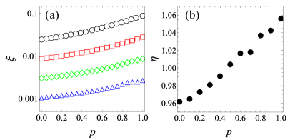
with the degree being the number of edges attached to node and ( otherwise). The clustering coefficient is the average [9] and thus is proportional to the number of triangles in the network. Figure 2(a) shows as a function of . It goes from , which corresponds to the AN () [12], to when the bit-1 subnetwork () is achieved [1]. The likelihood of broken links between both binary ANs increases with , diminishing the density of triangles in the network. However, we observe that remains considerably high, close to the level that corresponds to the standard AN, for probabilities as high as . Also note that the system size does not affect the curve.
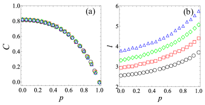
The other parameter that accounts for the small-world effect is the average shortest path length defined as
| (2) |
where is the length of the shortest path between nodes and . As can be seen in Fig. 2(b), slightly increases with , an expected tendency given the density of triangles is diminishing. The important feature to address here is how scales with . Assuming we find the exponent for all values of . Thus, the whole family of diluted ANs falls in an intermediate class between small () and ultrasmall [] networks.
So far we realize that the small-world character of the AN is resilient to the random deletion of nodes. In addition, only the clustering coefficient is affected by the dilution procedure. This suggests that the binary subnetworks are key building blocks of the standard AN.
Small-world networks with a power-law degree distribution are generally robust against attacks of that nature due to the presence of hubs [22]. In fact, the AN and the binary ANs are scale-free, a trait also portrayed by the diluted AN. The cumulative degree distribution is defined as
| (3) |
where is the number of sites with a certain degree at generation . Here we indeed observe that the diluted AN is scale free, as characterized by the asymptotic form , with for all .
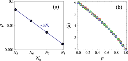
The scale-free attribute implies in the existence of a larger number of low-degree nodes that form dense communities linked through local hubs. In the standard AN most of the nodes have degree , precisely nodes for a given generation . In the bit-1 subnetwork () nodes have degree which signalizes its dendritic pattern. Both limiting networks are sparse in the sense that their average degree converges to a constant, namely (AN) and (1-bit AN) as [1].
The convergence of can be derived from the relationship , where is the connectance, that is the ratio between total number of edges and its maximum possible value (which corresponds to a fully connected network). For the whole range of we obtain , as depicted in Fig. 3(a). Hence, the diluted AN is also sparse, with varying with as seen in Fig. 3(b). Such behavior can be generated by the polynomial . Interestingly, so far as the structural properties discussed above are concerned, the diluted AN behaves much like the standard AN (up to intermediate values of ) despite having a distinct topology. For instance, when we have and the small-world property still preserved with and .
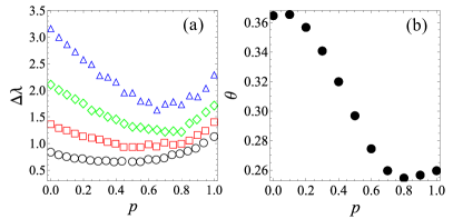
Let us now move on to discuss some spectral properties of the network, starting with the energy (eigenvalue) gap between the ground and the first excited states, . This is an important parameter that can be used to identify, e.g., quantum phase transitions [23]. It also plays a pivotal role in the critical behavior of Bose-Einstein condensates [16]. The energy gap versus is presented in Fig. 4(a). It is found to obey the power-law scaling , with the exponent behaving as shown in Fig. 4(b). The limiting cases (AN) (1-bit subnetwork) can be found elsewhere [16, 1]. The scaling behavior of the gap does not undergo relevant changes and its divergence relates to the ever increasing degree of the nodes belonging to the inner generations [24, 25]. It also deserves notice that the 1-bit subnetwork retains the original AN hub (see Fig. 1). In the 0-bit subnetwork, contrarily, as found in [1].
Last, we turn our attention to the ground-state eigenvector itself , which happens to feature remarkable localization properties. In scale-free networks with undirected edges the extreme eigenvectors are strongly localized at the hub [25].
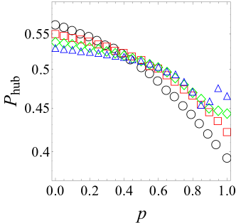
In Fig. 5 we plot the occupation probability at the hub versus with respect to , that is . We identify a transition between two regimes at about . Below this value, decreases as grows. This happens because even though is always strongly localized at the hub, reconfiguration of the network upon addition of a large number nodes at every new generation follows a self-similar pattern in the AN (). The unfolding rotation symmetry produce a highly structured and degenerate energy spectrum featuring a mix between extended and localized states, the degree of which typically depends on the node degree [14, 7]. Furthermore, for all considered the amplitude decays to a certain point with increasing . This trend can be associated to the rotation symmetry break and decrease in .
The 1-bit subnetwork, one the other hand, is bipartite [1]. Nodes can be grouped into two subsets, and , with no edges connecting nodes within the same subset. This arrangement satisfies [26]. As increases, this constraint and the scale-free property of the network render extreme eigenstates carrying approximately 50 of their amplitude at the hub as seen in Fig. 5 (see also Ref. [1]). The remaining is mostly distributed among its first low-degree neighbors. This tendency is further explored in Appendix A. A similar argument can be used to explain the apparent convergence in the AN case () as increases. It can be verified numerically that the components approach zero given in the adjacency matrix. Despite the lack of bipartite symmetry in the AN, its rotation symmetry and community structure ruled by sets of local hubs [7, 14] contribute to the onset of a gapped ground state (cf. Fig. 4) resembling that of a very dense star graph (see Fig. 7 and discussion in Appendix A) for higher generations .
Next, we want to analyze the localization degree of , whic can be done through the inverse participation ratio defined as . It yields for fully localized states and for extended states. Assuming , the decay coefficient quantifies the localization degree. In Figs. 6(a) and 6(b) we show both and against , respectively, the latter being throughout.
We confirm that in the midst of the departure from the AN rotation symmetry toward the tree-like form as the clustering coefficient fades, the ground state remains strongly localized. And the state has its highest amplitude at the node featuring the highest degree, as expected.
Conclusions. We have seen that the AN is quite robust against the random removal of nodes of the binary partition. Network properties such as the shortest path length and the degree distribution maintained their exponents and for all despite . We also observed no significant changes to the exponent associated to the gap between the ground and first excited states . One contributing factor to this is that the 1-bit subnetwork includes the hub (central node) of the original AN (see Fig. 1). The scaling of the gap influences, for instance, the critical temperature of a Bose-Einstein condensation in the AN [16].
In terms of the small-world property that presuppose a short and high , we remark that remains close to the level corresponding to the AN, , for values as high as . This is interesting if we contemplate how the AN topology is modified under the random attacks to the 0-bit partition. The diluted AN is always sparse with the average degree obeying , where . At , , indicating a dramatic change in the network topology.
We highlight that the symmetry underlying the diluted AN stands halfway between the rotation symmetry portrayed by the AN and the dendritic profile of the 1-bit partition. This pattern has been shown to be crucial in determining the hub amplitude in the ground state. Yet, its overall localization degree as computed via the inverse participation ratio yields , with for all . This, once again, confers robustness to the AN.
The binary AN subnetworks [1] are indeed key partitions that carry the essence of the standard AN [12]. Interpolating between them broadens the range of applicability, specially if a tunable clustering coefficient is desired. Further studies directed toward the modeling of real-world networks and other complex systems using the diluted AN class are timely.
The authors thank A. M. C. Souza and L. K. Souza for sharing key insights. This work was supported by CNPq (Brazilian agency) and FAPEAL (Alagoas State agency).
Appendix A Competing hubs in dendritic networks
In this section we devise a toy model to explain why the probability amplitude of the 1-bit subnetwork hub in the ground state tends to as increases.
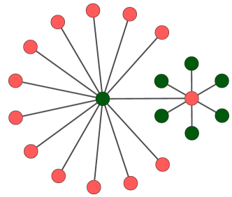
Let us consider two star networks coupled via their respective central nodes (local hubs) and , with degrees and , as depicted in Fig. 7. The nodes are marked with different colors to highlight the disjoint sets and due to the bipartite property of the network. The total number of nodes is thus . Once again, we assume a symmetric adjacency matrix with non-zero elements only if an edge connects nodes and .
Each star network is itself bipartite as well. By carrying out a partial diagonalization, each one delivers () zero-energy eigenstates having null amplitude at the star center and two others with energies :
| (4) |
where is an even linear combination of the nodes attached to the corresponding star center.
The components of the non-zero eigenstates are divided such that there is a chance to find a particle at the center or distributed over the other disjoint set, in accordance to [26]. Another theorem [27] has it that in every bipartite network there should be at least a number of zero-energy eigenstates that equals the difference between the number of nodes belonging to each disjoint set. And these states will have no amplitude in the minority set.
Returning to the coupled scenario (as in Fig. 7), we realize that the zero and non-zero eigenstates as obtained above do not mix because both parts are connected via their local hubs. That is, . As such, the four states span their own eigenspace. We now proceed with a change of basis to the set to express the effective adjacency matrix (written in that order) as
| (5) |
Surprisingly, we are able to express the coupled star network system of Fig. 7 as a linear chain in the state sector that contains each star center. Similar structures can be found within networks that exhibits dendritic (tree-like) patterns such as the binary ANs [1]. Solving the eigenvalue equation for , we obtain
| (6) |
where and . The corresponding eigenvectors have the form
| (7) |
where is a normalization factor.
In the effective 4-node network, () pair up with () with respect to disjoint bipartite subsets. Accordingly, we must have , with [26]. This can be regarded as a competition between one star center and the nodes adjacent to the other in order to fulfill the occupation probability allocated for them.
In a situation in which, say , the eigenvalues [Eq. (6)] approach and . After some algebraic manipulation on Eq. (7) we find that the extreme eigenstates (they are indeed associated to the node with the highest degree). Therefore, as .
To summarize, whenever one of the star networks becomes very dense, it effectively splits apart from the other. Notwithstanding that the 1-bit AN subnetwork has a much more complex topology, the above picture captures the essence of the behavior seen in Fig. 5 in the unclustered limit () as grows.
References
- [1] E. M. K. Souza, and G. M. A. Almeida, Phys. Rev. E 107, 024305 (2023).
- [2] S. Boccaletti, V. Latora, Y. Moreno, M. Chavez, and D.-U. Hwang, Phys. Rep. 424, 175 (2006).
- [3] J. A. Firth, J. Hellewell, P. Klepac, S. Kissler, A. J. Kucharski, and L. G. Spurgin, Nat. Med. 26, 1616 (2020).
- [4] S. N. Dorogovtsev, A.V. Goltsev, and J. F. F. Mendes, Phys. Rev. E 65, 066122 (2002).
- [5] M. E. J. Newman, Phys. Rev. E 64, 016131 (2001).
- [6] V. Latora and M. Marchiori, Physica A 314, 109 (2002).
- [7] G. M. A. Almeida and A. M. C. Souza, Phys. Rev. A 87, 033804 (2013).
- [8] J. Biamonte, M. Faccin, and M. De Domenico, Commun. Phys. 2, 53 (2019).
- [9] D. J. Watts and S. H. Strogatz, Nature 393, 440 (1998).
- [10] A.-L. Barabási and R. Albert, Science 286, 509 (1999).
- [11] P. Erdös and A. Rényi, Publ. Math. Inst. Hung. Acad. Sci. 5, 17 (1960).
- [12] J. S. Andrade Jr., H. J. Herrmann, R. F. S. Andrade, and L. R. da Silva, Phys. Rev. Lett. 94, 018702 (2005).
- [13] R. F. S. Andrade and H. J. Herrmann, Phys Rev. E 71, 056131 (2005).
- [14] A. L. Cardoso, R. F. S. Andrade, and A. M. C. Souza, Phys. Rev. B 78 214202 (2008).
- [15] I. N. de Oliveira, F. A. B. F. de Moura, M. L. Lyra, J. S. Andrade Jr., and E. L. Albuquerque, Phys. Rev. E 79, 016104 (2009).
- [16] I. N. de Oliveira, F. A. B. F. de Moura, M. L. Lyra, J. S. Andrade, Jr., and E. L. Albuquerque, Phys. Rev. E 81, 030104(R) (2010).
- [17] X.-P. Xu, W. Li, and F. Liu, Phys. Rev. E 78, 052103 (2008).
- [18] T. Zhou, G. Yan, and B.-H. Wang, Phys. Rev. E 71, 046141 (2005).
- [19] P. Holme, B. J. Kim, C. N. Yoon, and S. K. Han, Phys. Rev. E 65, 056109 (2002).
- [20] Q. K. Teleford, K. E. Joyce, H. Satoru, J. H. Burdette, and P. J. Laurienti, Brain Connectivity 1, 367 (2011).
- [21] M. Boguñá, D. Krioukov, P. Almagro, and M. A. Serrano, Phys. Rev. Research 2, 023040 (2020).
- [22] R. Cohen, K. Erez, D. ben-Avraham, and S. Havlin, Phys. Rev. Lett. 85, 4626 (2000).
- [23] C. Presilla and M. Ostilli, Physica A 515, 57 (2019).
- [24] N. Alon, Combinatorica 6, 83 (1986).
- [25] K.-I. Goh, B. Kahng, and D. Kim, Phys. Rev. E 64, 051903 (2001).
- [26] A. M. C. Souza, R. F. S. Andrade, N. A. M. Araujo, A. Vezzani, and H. J. Herrmann, Phys. Rev. E 95, 042130 (2017).
- [27] M. Inui, S. A. Trugman, and E. Abrahams, Phys. Rev. B 49, 3190 (1994).