Scalable Lipschitz Estimation for CNNs

Abstract

Estimating the Lipschitz constant of deep neural networks is of growing interest as it is useful for informing on generalisability and adversarial robustness. Convolutional neural networks (CNNs) in particular, underpin much of the recent success in computer vision related applications. However, although existing methods for estimating the Lipschitz constant can be tight, they have limited scalability when applied to CNNs. To tackle this, we propose a novel method to accelerate Lipschitz constant estimation for CNNs. The core idea is to divide a large convolutional block via a joint layer and width-wise partition, into a collection of smaller blocks. We prove an upper-bound on the Lipschitz constant of the larger block in terms of the Lipschitz constants of the smaller blocks. We demonstrate an enhanced scalability and comparable accuracy to existing baselines through a range of experiments.

1 Introduction

It has been shown that deep neural networks (DNNs) exhibit vulnerabilities to adversarial attacks (Goodfellow et al., 2014; Madry et al., 2018), which in the field of image classification are defined by imperceptible changes to the input image resulting in misclassification. In recent years, there has been an increased effort to develop methods to measure the robustness of DNNs to such attacks. One way to do so is through accurate estimation of the Lipschitz constant of neural networks (Akhtar & Mian, 2018). Given a function $f:\mathbb{R}^{n}\to\mathbb{R}^{m}$, we say $f$ is globally Lipschitz continuous with respect to a norm $\|\cdot\|$, if $\exists L\geq 0$ such that:

$$\|f(\mathbf{x})-f(\mathbf{y})\|\leq L\|\mathbf{x}-\mathbf{y}\|,\,\forall\,\mathbf{x},\mathbf{y}\in\mathbb{R}^{n}.$$ (1)

The minimum value of $L$ for which (1) holds is called the Lipschitz constant of $f$, denoted by $L(f)$. It intuitively provides a metric for measuring adversarial robustness, as it gives the maximum ratio between changes in the output space with respect to changes in the input space.

Existing methods for Lipschitz estimation of DNNs are either scalable but conservative (Szegedy et al., 2014), or accurate in their estimation but unable to scale to larger networks (Fazlyab et al., 2019; Latorre et al., 2019; Raghunathan et al., 2018), due to the underlying optimisation problems. For example, the LipSDP method (Fazlyab et al., 2019) formulates (1) as a semidefinite program (SDP). Classical interior-point methods (Vandenberghe & Boyd, 1996) deployed for solving such problems have a per-iteration time complexity of $\mathcal{O}(N^{3}m+N^{2}m^{2}+m^{3})$ and a memory complexity of $\mathcal{O}(N^{2}+m^{2})$, where $N$ denotes the size of the constraint matrix and $m$ the number of equality constraints. On regular computers, computational bottlenecks are reached for problems with $N$ and $m$ greater than a few hundred and thousand respectively (Zheng et al., 2021; Majumdar et al., 2020). This becomes problematic when applying the LipSDP method to convolutional neural networks (CNNs) due to the significant increase of problem size caused by CNNs.

Current acceleration methods exploit parallelisation (Fazlyab et al., 2019) or sparsity patterns in the underlying SDP (Xue et al., 2022) to scale to deeper networks, but not necessarily wider ones. With the growing use of deep and wide CNNs in safety-critical domains (Bojarski et al., 2016; Esteva et al., 2017), it is important to provide practitioners with both an accurate and scalable way to measure the Lipschitz constant. Our contributions include:

• We propose a novel method, named as dynamic convolutional partition (DCP), for scaling existing Lipschitz estimation frameworks to deep and wide CNNs, by dividing a large convolutional block into a collection of smaller blocks via a joint layer and width-wise partition.

• We prove that the Lipschitz constant of a large convolutional block can be bounded above by the Lipschitz constants of the smaller blocks, serving as the theoretical foundation for our acceleration method.

• We demonstrate an enhanced scalability and comparable accuracy of our method over existing baselines, through a range of experiments.

2 Related Works

The earliest attempt at estimating the global Lipschitz constant of neural networks (NNs) was made by Szegedy et al. (2014). They bound the Lipschitz constant above in terms of the product of the spectral norm of the weight matrices at each layer, i.e. $L=\prod_{i=1}^{l}\|\mathbf{W}_{i}\|_{2}$, by using a well-known result described in our later section by Lemma 3.1. While scalable, this approach yields conservative bounds for non-linear networks, and is sometimes referred to by existing literature as a naive estimation (Fazlyab et al., 2019; Xue et al., 2022). Recently, methods for exactly computing the spectral norm of convolutional layers have been developed (Sedghi et al., 2018; Singla & Feizi, 2021). Another layer-based approach estimates the Lipschitz constant through the singular value decomposition of the weight matrices and the maximisation of the activation gradients, known as SeqLip (Scaman & Virmaux, 2018). However, it uses a brute force approach, which becomes impractical for larger networks. Tighter bounds have been developed by Combettes & Pesquet (2020) based on abstracting activation functions as averaged operators, but this method scales exponentially with network depth.

An alternative direction providing tighter bounds poses the problem of Lipschitz constant estimation as a linear program or SDP through convex relaxations. For instance, Raghunathan et al. (2018) estimate the Lipschitz constant of NNs with a single hidden layer by solving an SDP with respect to the $\ell_{\infty}$-norm. This was later shown by Latorre et al. (2019) to be a specific relaxation of their method LiPopt, a linear program framework for estimating the local Lipschitz constant. LipSDP (Fazlyab et al., 2019) is considered the state of the art for estimating the global Lipschitz constant. It is based on characterising the activation functions as quadratic constraints (Açıkmeşe & Corless, 2011) to develop an SDP for minimising the upper bound of the Lipschitz constant of a feedforward neural network (FNN). Recently, SDP variations have been developed based on dissipativity theory for 1-D and 2-D convolutional neural networks (Pauli et al., 2023; Gramlich et al., 2023).

The main disadvantage of SDP-based estimation schemes is the computational bottleneck associated with interior-point methods when optimising with respect to a large constraint matrix. In an attempt to offset this, Fazlyab et al. (2019) proposed a hierarchy of relaxations based on varying the number of decision variables, allowing a trade-off between scalability and accuracy. However, their relaxation based on fully-dense matrices (LipSDP-Network) was later disproven by Pauli et al. (2021). To exploit parallelisation, Fazlyab et al. (2019) also suggested a layer-wise cutting approach to decompose an FNN into a collection of subnetworks, and upper bounded the Lipschitz constant in terms of the Lipschitz constants of these smaller subnetworks. Although this is effective in improving scalability to deeper networks, it does not improve the computational tractability to wider layers. Recently, Chordal-LipSDP (Xue et al., 2022) has been proposed to accelerate by decomposing a large constraint matrix into an equivalent sum of smaller ones, encouraged by theory relating sparse matrices and chordal graphs (Agler et al., 1988; Vandenberghe et al., 2015). However, their experiments are somewhat limited by only considering FNNs of an input dimension of 2 and a maximum hidden width of 50. Another potential drawback of Chordal-LipSDP is that their vanilla chordal decomposition ignores the increase in the number of equality constraints, and this can potentially nullify the computational benefits of optimising over smaller constraint matrices (Fukuda et al., 2001; Garstka et al., 2020). To the best of our knowledge, there is no existing acceleration method in the field that works effectively for both deep and wide neural networks.

3 Preliminaries

We denote matrices and vectors as bold face capital and lower-case letters respectively. The vector space of $n\times n$ symmetric matrices and the cone of $n\times n$ symmetric, positive semidefinite (PSD) matrices are denoted by $\mathbb{S}^{n}$ and $\mathbb{S}_{+}^{n}$, respectively. We will write $\mathbf{X}\succeq 0$ instead of $\mathbf{X}\in\mathbb{S}_{+}^{n}$. We use $\|\cdot\|_{p}$ to denote the vector $p$-norm. The inner product between two vectors $\mathbf{x},\mathbf{y}\in\mathbb{R}^{n}$, is denoted by $\langle\mathbf{x},\mathbf{y}\rangle=\mathbf{x}^{\top}\mathbf{y}$. The $n$-dimensional identity matrix is denoted by $\mathbf{I}_{n}$. $\mathcal{I}$ denotes the set of positive indices and $|\mathcal{I}|$ is its cardinality.

In this paper, we study CNNs consisting of convolutional layers taking equal input height and width of $n_{i}$ and channel size $c_{i}$ and of fully-connected layers taking input size of $N_{i}$. We consider their re-characterisation as FNNs consisting of flattened convolutional layers $C_{i}:\mathbb{R}^{c_{i-1}n_{i-1}^{2}}\to\mathbb{R}^{c_{i}n_{i}^{2}}$ with indices $i\in\mathcal{I}_{\mathcal{C}}$ and fully-connected layers $\mathcal{F}_{i}:\mathbb{R}^{N_{i-1}}\to\mathbb{R}^{N_{i}}$ with indices $i\in\mathcal{I}_{\mathcal{F}}$. We refer to the convolutional layers as a convolutional block. The resulting FNN can be recursively expressed as follows:

$$f\left(\mathbf{x}^{0}\right)= \;\mathbf{W}^{\ell}\mathbf{x}^{\ell-1}+\mathbf{b}^{\ell},$$

$$\mathbf{x}^{i}= \;\phi\left(\mathbf{W}^{i}\mathbf{x}^{i-1}+\mathbf{b}^{i}\right),i=1,2,\ldots,\ell-1,$$ (2)

where $\ell=|\mathcal{I}_{\mathcal{C}}|+|\mathcal{I}_{\mathcal{F}}|$. Here, $\mathbf{W}^{i},\mathbf{b}^{i}$ are the weight and bias respectively, applied at the $i$-th layer. The activation function $\phi(\cdot)$ is non-linear and applied component-wise, e.g., ReLU and tanh. We apply the same activation function at each layer unless stated otherwise.

3.1 Lipschitz Bounds

We first present some well-known results from functional analysis (Cobzaş et al., 2019) that serve as the theoretical foundation for our method.

Lemma 3.1.

The Lipschitz constant of a composite function $f(x)=(g_{k}\circ g_{k-1}\circ\ldots\circ g_{1})(x):\mathbb{R}^{n}\to\mathbb{R}^{m}$ is bounded above by

$$L(f)\leq\prod_{i=1}^{k}L(g_{i}).$$ (3)

The above result also underpins the layer-wise cutting approach proposed by Fazlyab et al. (2019). The proceeding lemma bounds the Lipschitz constant of a multivariate, vector-valued function in terms of its component functions.

Lemma 3.2.

Given a function $f:A\to\mathbb{R}^{m}$ where $A\subseteq\mathbb{R}^{n}$, let $f_{i}:A\to\mathbb{R}$ denote its $i$-th component such that $f=[f_{1},f_{2},\ldots f_{m}]^{\top}$. Considering $l_{2}$-norm, the Lipschitz constant of $f$ is bounded above by

$$L(f)\leq\Biggl{(}\sum_{i=1}^{m}L(f_{i})^{2}\Biggr{)}^{\frac{1}{2}},$$ (4)

3.2 LipSDP Framework

We briefly outline the LipSDP framework (Fazlyab et al., 2019), which we will use to demonstrate the effectiveness of our method. It characterises the activation functions as incremental quadratic constraints, predicated on the fact that they are slope-restricted on $[s_{1},s_{2}]$, i.e. the slope of the secant line connecting any two points is bounded below and above by $s_{1}$ and $s_{2}$ respectively, where $0\leq s_{1}<s_{2}<\infty$. As a result, a tight upper bound on the Lipschitz constant of an FNN recursively expressed by (2) can be found by solving the following optimisation problem over the bound value $L$ and a symmetric matrix $\mathbf{T}$:

$$\min_{L\geq 0,\mathbf{T}\in\mathbb{T}_{N}}\;L^{2},$$ (5)

$$\textrm{subject to}\;\mathbf{M}\left(L^{2},\mathbf{T}\right)\preceq 0.$$

The dimension of $\mathbf{T}$, denoted by $N$, is equal to the total number of hidden neurons, and its search space $\mathbb{T}_{N}\subset\mathbb{S}^{N}$ can be restricted to the set of all non-negative diagonal matrices. The constraint matrix $\mathbf{M}\coloneqq\mathbf{M}_{1}(\mathbf{T})+\mathbf{M}_{2}\left(L^{2}\right)$ is a square matrix of a larger dimension $N_{0}+N$, where $N_{0}$ denotes the number of input neurons, and

$$\mathbf{M}_{1}= \;\begin{bmatrix}\mathbf{A}\\ \mathbf{B}\\ \end{bmatrix}^{\top}\begin{bmatrix}-2s_{1}s_{2}\mathbf{T}&(s_{1}+s_{2})\mathbf{T}\\ (s_{1}+s_{2})\mathbf{T}&2\mathbf{T}\\ \end{bmatrix}\begin{bmatrix}\mathbf{A}\\ \mathbf{B}\\ \end{bmatrix},$$ (6)

$$\mathbf{M}_{2}= \;\begin{bmatrix}-L^{2}\mathbf{I}_{N_{0}}&\mathbf{0}&\ldots&\mathbf{0}\\ \mathbf{0}&\mathbf{0}&\ldots&\mathbf{0}\\ \vdots&\vdots&\ddots&\vdots\\ \mathbf{0}&\mathbf{0}&\ldots&(\mathbf{W}^{\ell})^{\top}\mathbf{W}^{\ell}\\ \end{bmatrix},$$ (7)

also

$$\mathbf{A}=\begin{bmatrix}\mathbf{W}^{1}&\ldots&\mathbf{0}&\mathbf{0}\\ \vdots&\ddots&\vdots&\vdots\\ \mathbf{0}&\ldots&\mathbf{W}^{\ell-1}&\mathbf{0}\\ \end{bmatrix},\,\mathbf{B}=\begin{bmatrix}\mathbf{0}&\mathbf{I}_{N_{1}}&\ldots&\mathbf{0}\\ \vdots&\vdots&\ddots&\vdots\\ \mathbf{0}&\mathbf{0}&\ldots&\mathbf{I}_{N_{l}}\\ \end{bmatrix}.$$ (8)

It can be seen that $\mathbf{M}\left(L^{2},\mathbf{T}\right)$ is linear in $L^{2}$ and $\mathbf{T}$.

4 Methodology

We propose the DCP method for accelerating Lipschitz estimation of CNNs, designed to address the depth and width of the network. In summary, it works by exploiting the fact that the network can be characterised by vector-valued composite functions. From this, Lemma 3.1 allows us to express the network as a collection of subnetworks. Lemma 3.2 allows us to partition each subnetwork into smaller convolutional blocks, which are independent meaning that their Lipschitz constants can be computed in parallel. We outline how to upper bound the Lipschitz constant of the original convolutional block in terms of the Lipschitz constants of the smaller blocks. Further details are provided in the proceeding sections.

4.1 Dynamic Convolutional Partition

4.1.1 Convolutional Partitioning

We first present convolutional partitioning, proposed to handle large network width. Given a function $F:\mathbb{R}^{n_{0}\times n_{0}\times c_{0}}\to\mathbb{R}^{n_{\ell}\times n_{\ell}\times c_{\ell}}$ characterising an $\ell$-layer convolutional block, we begin by partitioning the integer $n_{\ell}$ into $d$-parts through the computation of a restricted integer composition (RIC) (Heubach & Mansour, 2004). We refer to $d$ as the partition factor. A RIC of $n_{\ell}$, which we denote by $R^{n_{\ell}}_{d}$, is of the form $n_{\ell}=\sum_{i=1}^{d}p_{i}$, where $p_{i}$ denotes the $i$-th part. The partition factor is in the range $1<d\leq n_{\ell}$, noting that $d=1$ corresponds to applying no partition. Each part is strictly positive and at most $n_{\ell}-(d-1)$, which arises when $(d-1)$ parts are equal to one. Letting $\mathbf{X}^{\ell}$ denote the output of the final convolutional layer, a given RIC divides $\mathbf{X}^{\ell}$ into a $d\times d$ grid by

$$\mathbf{X}^{\ell}=\begin{bmatrix}\mathbf{X}_{11}^{\ell}&\mathbf{X}_{12}^{\ell}&\cdots&\mathbf{X}_{1d}^{\ell}\\ \mathbf{X}_{21}^{\ell}&\mathbf{X}_{22}^{\ell}&\cdots&\mathbf{X}_{2d}^{\ell}\\ \vdots&\vdots&\ddots&\vdots\\ \mathbf{X}_{d1}^{\ell}&\mathbf{X}_{d2}^{\ell}&\cdots&\mathbf{X}_{dd}^{\ell}\end{bmatrix},$$ (9)

where $\mathbf{X}_{ij}^{\ell}\in\mathbb{R}^{p_{i}\times p_{j}\times c_{\ell}}$. We then identify the neurons in the input layer contributing to each $\mathbf{X}_{ij}^{\ell}$ denoting them $\mathbf{X}_{ij}^{0}$. Applying the subsequent convolutional operators forms the functions $\mathbf{X}_{ij}^{\ell}=f_{ij}\left(\mathbf{X}_{ij}^{0}\right)$. This allows us to express $F$ as smaller convolutional blocks as follows:

$$F(\mathbf{X}^{0})=\begin{bmatrix}f_{11}\left(\mathbf{X}_{11}^{0}\right)&\cdots&f_{1d}(\mathbf{X}_{1d}^{0})\\ \vdots&\ddots&\vdots\\ f_{d1}\left(\mathbf{X}_{d1}^{0}\right)&\cdots&f_{dd}\left(\mathbf{X}_{dd}^{0}\right)\end{bmatrix}.$$ (10)

By design, any two distinct output blocks $\mathbf{X}_{ij}^{\ell}$ and $\mathbf{X}_{pq}^{\ell}$ are disjoint but can in general share input neurons.

Next, we flatten the partitioned convolutional block (10) using the standard vectorisation operation by first flattening each input sub-matrix, i.e. $\mathbf{x}_{ij}^{0}\coloneqq vec(\mathbf{X}_{ij}^{0})$, concatenating the resulting vectors to give $\mathbf{x}^{0}=[\mathbf{x}_{11}^{0},\mathbf{x}_{12}^{0},\ldots,\mathbf{x}_{dd}^{0}]$. Then we vectorise each smaller convolutional block, i.e. $\widetilde{f}_{ij}:\mathbb{R}^{n_{i}^{0}n_{j}^{0}c_{0}}\to\mathbb{R}^{p_{i}^{0}p_{j}^{0}c_{\ell}}$, where $\widetilde{f}_{ij}=vec(f_{ij})$. The flattened, partitioned convolutional block is then given by:

$$F_{u}(\mathbf{x}^{0})=\left[\widetilde{f}_{11}\left(\mathbf{x}_{11}^{0}\right),\widetilde{f}_{12}\left(\mathbf{x}_{12}^{0}\right),\ldots,\widetilde{f}_{dd}\left(\mathbf{x}_{dd}^{0}\right)\right].$$ (11)

The sparse structure of the flattened convolutional layers permits a significant reduction in size of each flattened convolutional block. Exploiting this redundancy underpins our method.

Based on Lemma 3.2, we derive that the Lipschitz constant of $F_{u}$ can be bounded above in terms of the Lipschitz constants of $\{\widetilde{f}_{ij}\}_{i,j=1}^{d}$ from (11). The result is formalised in the following theorem.

Theorem 4.1.

Given a function $F:\mathbb{R}^{n_{0}\times n_{0}\times c_{0}}\to\mathbb{R}^{n_{\ell}\times n_{\ell}\times c_{\ell}}$ characterising an $\ell$-layer convolutional block and its flattened, partitioned form given by (11). Then $L(F_{u})$ is bounded above by

$$L(F_{u})\leq\Biggl{(}\sum_{i,j=1}^{d}L\left(\widetilde{f}_{ij}\right)^{4}\Biggr{)}^{\frac{1}{4}}.$$ (12)

A proof is given in Section A.2 of the supplementary material. Theorem 4.1 provides us with a sufficient condition for bounding the Lipschitz constant of a larger convolutional block above, in terms of the Lipschitz constants of $d^{2}$ smaller blocks obtained via partitioning. A key advantage is that each $L(\widetilde{f}_{ij})$ can be computed in parallel, enabling efficient implementation in practice.

4.1.2 Joint Layer and Width-Wise Partitioning

To handle both deep and wide CNNs, we combine our convolutional partitioning with layer-wise cutting. We incorporate Lemma 3.1 to express $F$ as the composition of $s$ subnetworks, characterised by the set of ordered integers $\mathcal{C}_{s}=\{I_{0},I_{1},\ldots,I_{s-1},I_{s}\}$, such that $0=I_{1}<I_{1}<\ldots<I_{s}=\ell$, where a pair of consecutive integers $(I_{k-1},I_{k})$ denote the input and output layer respectively, of the $k$-th subnetwork, for $k\in\{1,2,\ldots,s\}$. For instance, given an 8-layer convolutional block, $\mathcal{C}_{3}=\{0,3,5,8\}$ cuts the block into 3 subnetworks at layer 3 and layer 5, and $(5,8)$ corresponds to the last subnetwork. Each subnetwork is partitioned into $d_{k}^{2}$ smaller convolutional blocks via the process outlined in Section 4.1.1. In this way we express $F$ as the following composite function:

$$F\left(\mathbf{X}^{0}\right)=(F_{s}\circ F_{s-1}\circ\ldots F_{1})\left(\mathbf{X}^{0}\right),$$ (13)

where the $k$-th individual function is given as follows:

$$F_{k}\left(\mathbf{X}^{I_{k-1}}\right)=\begin{bmatrix}f_{11}^{(k)}\left(\mathbf{X}_{11}^{I_{k-1}}\right)&\cdots&f_{1d_{k}}^{(k)}\left(\mathbf{X}_{1d_{k}}^{I_{k-1}}\right)\\ \vdots&\ddots&\vdots\\ f_{d_{k}1}^{(k)}\left(\mathbf{X}_{d_{k}1}^{I_{k-1}}\right)&\cdots&f_{d_{k}d_{k}}^{(k)}\left(\mathbf{X}_{d_{k}d_{k}}^{I_{k-1}}\right)\end{bmatrix}.$$ (14)

Here $\mathbf{X}^{I_{k-1}}$ denotes the output and input of the $(k-1)$-th and $k$-th subnetworks, respectively. The function $f_{ij}^{(k)}$ denotes the $(i,j)$-th convolutional block of the $k$-th subnetwork, for $1\leq i,j\leq d_{k}$. By flattening each individual function defined by (14), $F_{u}$ can be expressed as follows:

$$F_{u}\left(\mathbf{x}^{0}\right)=(F_{s}^{u}\circ F_{s-1}^{u}\circ\ldots F_{1}^{u})\left(\mathbf{x}^{0}\right),$$ (15)

where, for $k=1,2,\ldots,s$, we have:

$$F_{k}^{u}\left(\mathbf{x}^{I_{k-1}}\right)=\bigg{[}\widetilde{f}_{11}^{(k)}\left(\mathbf{x}_{11}^{I_{k-1}}\right),\widetilde{f}_{12}^{(k)}\left(\mathbf{x}_{12}^{I_{k-1}}\right),\ldots,\widetilde{f}_{d_{k}d_{k}}^{(k)}\left(\mathbf{x}_{d_{k}d_{k}}^{I_{k-1}}\right)\bigg{]}.$$ (16)

By way of Lemma 3.1 and the fact that Theorem 4.1 is applicable to each subnetwork $F_{k}^{u}$, we are able to bound the Lipschitz constant of $F_{u}$ in terms of the Lipschitz constants of the smaller convolutional blocks comprising each subnetwork. The result is formalised in the following corollary.

Corollary 4.2.

Given a function $F:\mathbb{R}^{n_{0}\times n_{0}\times c_{0}}\to\mathbb{R}^{n_{\ell}\times n_{\ell}\times c_{\ell}}$ characterising an $\ell$-layer convolutional block and its flattened, partitioned form $F_{u}$ expressed as the composition of $s$ subnetworks, as defined by (15). Then $L(F_{u})$ is bounded above as follows:

$$L(F_{u})\leq\prod_{k=1}^{s}\Biggl{(}\sum_{i,j=1}^{d_{k}}L\left(\widetilde{f}_{ij}^{(k)}\right)^{4}\Biggr{)}^{\frac{1}{4}}.$$ (17)

A proof is provided in Section A.3 of the supplementary material.

4.1.3 Dynamic Partition Search

Determining the optimal subnetwork decomposition $\mathcal{C}_{s}$, the set of partition factors $\{d_{k}\}_{k=1}^{s}$ and the corresponding set of RICs $\left\{R^{n_{\ell_{k}}}_{d_{k}}\right\}_{k=1}^{s}$, is non-trivial in general. Optimality here is defined as the choice of the aforementioned parameters giving the tightest upper bound on $L(F_{u})$, while ensuring that the Lipschitz estimation framework of choice does not exceed the available computational resource for any of the subnetworks. We describe this by the following optimisation problem:

$$\min_{\mathcal{C}_{s},\{d_{k}\}_{k=1}^{s},\left\{R^{n_{\ell_{k}}}_{d_{k}}\right\}_{k=1}^{s}} \;\;\prod_{k=1}^{s}\Biggl{(}\sum_{i,j=1}^{d_{k}}L\left(\widetilde{f}_{ij}^{(k)}\right)^{4}\Biggr{)}^{\frac{1}{4}},$$

s.t. $$\;\;P\left(A_{\textmd{Lip}},\widetilde{f}_{ij}^{k}\right)\leq P_{\max},\textmd{for }k=1,2,\ldots,s,\textmd{ and }i,j=1,2,\ldots d_{k}.$$ (18)

Here $P\left(A_{\textmd{Lip}},\widetilde{f}_{ij}^{k}\right)$ denotes the computational resource required by the Lipschitz estimation framework $A_{\textmd{Lip}}$, to compute the Lipschitz constant of $\widetilde{f}_{ij}^{k}$. $P_{\max}$ denotes the maximum available computing power. It is practically infeasible to find the global optimal solution to (4.1.3), so we deploy a dynamic search strategy aimed at balancing estimation accuracy and scalability. This involves: $(1)$ an empirical approximation of solution feasibility, $(2)$ a reduction of the search space of RICs, and $(3)$ a dynamic backwards search to determine a joint layer and width-wise partition. We note that these added relaxations give a Lipschitz upper-bound but not necessarily the global optimum. We expand on each design feature below.

Feasibility Examination. The computing power required by LipSDP is predominantly determined by the dimension of the square constraint matrix $\mathbf{M}$, which we recall is equal to the sum of the input and hidden neurons. Thus, we convert the constraint in (4.1.3) to the following constraint, which is simpler and practically easier to examine:

$$\max_{i,j,k}N\left(\widetilde{f}_{ij}^{k}\right)\leq N_{\max},$$ (19)

where $N(\cdot)$ denotes the constraint dimension associated with the input network and $N_{\max}$ the maximally allowed dimension. In practice, we can empirically estimate $N_{\max}$ by performing multiple simulations, whereby SDPs of increasing size are generated and the constraint dimension for which computational bottlenecks are reached is recorded. Averaging over all such instances gives an estimate of $N_{\max}$. In Section A.5.1, we discuss cheaper ways to obtain an estimation.

RIC Space Reduction. Enumerating all possible RICs of $n_{\ell}$ is computationally prohibitive as $n_{\ell}$ increases (Eger, 2013). To reduce the search cost we impose the additional constraint whereby different orderings of the same composition are considered non-distinct. This is formally referred to as a restricted integer partition (RIP) (Andrews & Eriksson, 2004). For example, given $n_{\ell}=5$ and $d=2$, the set of RICs of $n_{\ell}$ into two parts is $\{(1,4),(2,3),(3,2),(4,1)\}$, while the set of RIPs is given by $\{(1,4),(2,3)\}$. We sort all RIPs lexicographically. For example, given $n_{\ell}=8$ and $d=3$ the lexicographically ordered set of RIPs is $\{(1,1,6),(1,2,5),(1,3,4),(2,2,4),(2,3,3)\}$. Polynomial-time algorithms for computing integer compositions and restrictions are detailed in Opdyke (2010); Vajnovszki (2013).

Backward Partition Search. As outlined in Section 4.1.1, we partition the original convolutional block in a backwards manner, i.e., starting from the last layer, to ensure that the resulting subnetworks $\{\widetilde{f}_{ij}^{k}\}_{i,j,k}$ do not have overlapping outputs, which is required to develop the result in Corollary 4.2. When working with the LipSDP framework, networks require at least one hidden layer (Theorem 1; Fazlyab et al. (2019)). Thus, we begin by considering the subnetwork indexed by $(\ell-2,\ell)$. We choose a suitable partition factor in an iterative manner, starting at $2$ and incrementing to $n_{\ell}$ if necessary. For a given value of $d$, we select a RIP of $n_{\ell}$ into $d$-parts following the lexicographical order and check if (19) is satisfied. If the criterion is not met for any element in the RIP set, we increment $d$ and repeat the process. Otherwise, we choose the first element for which it is satisfied and perform a backwards pass across the network using this RIP choice, considering the subnetwork indexed by $(\ell-k,\ell)$ for $k\in\{3,\ldots,\ell\}$. If the constraint is violated at layer $k$, then $(\ell-k+1,\ell)$ forms the first subnetwork and the $(\ell-k+1)$-th layer is taken as the output of the proceeding subnetwork. Repeating this process until the input layer, forms a collection of $s$ subnetworks, each comprised of smaller (flattened) convolutional blocks. This process is outlined in Algorithm 1 in Section A.1. It prioritises finding a partition choice that does not violate the computing constraint, while the use of lexicographical order favours the selection of an RIP with a bigger size difference among the parts. As we show in Section 5.2, this can potentially encourage a tighter upper-bound.

4.2 Scalability Analysis

To establish an understanding of the effectiveness of the proposed DCP method in improving scalability, we analyse sufficient conditions to achieve the best and worst-case reductions in time complexity. This analysis is based on the per-iteration time complexity of classical interior-points methods, i.e. $\mathcal{O}(N^{3}m+N^{2}m^{2}+m^{3})$, where $N$ and $m$ denote the dimension of the linear matrix inequality (LMI) and the number of equality constraints, respectively, in (5). Given a convolutional block $F:\mathbb{R}^{n_{0}\times n_{0}\times c_{0}}\to\mathbb{R}^{n_{\ell}\times n_{\ell}\times c_{\ell}}$, $m$ is equal to one and $N=\sum_{i=0}^{\ell-1}c_{i}n_{i}^{2}$. The following proposition informs of the best and worst-case reductions in time complexity.

Proposition 4.3.

Given an $\ell$-layer convolutional block $F:\mathbb{R}^{n_{0}\times n_{0}\times c_{0}}\to\mathbb{R}^{n_{\ell}\times n_{\ell}\times c_{\ell}}$ and a $d$-part RIP of $n_{\ell}$, i.e. $n_{\ell}=\sum_{i=1}^{d}p_{i}$, we consider the largest block after the partition i.e., $\rho_{*}=\max_{i=1}^{d}p_{i}$ and its associated constraint dimension $N_{*}$. Then we have the following cases:

1. Best-case. When $d=n_{\ell}$ and $\rho_{*}=1$ by direct consequence, it has

   $$\bigg{(}\frac{N_{*}}{N}\bigg{)}^{3}=O\bigg{(}\frac{1}{n_{\ell}^{6}}\bigg{)},\,\textrm{as}\,n_{\ell}\rightarrow\infty.$$ (20)

2. Worst-case. When $d=2$ with $\rho_{*}=\lceil\frac{n_{\ell}}{2}\rceil$, it has

   $$\bigg{(}\frac{N_{*}}{N}\bigg{)}^{3}=O(1).$$ (21)

Intuitively the best case reduction corresponds to the minimum possible size of the largest convolutional block after partitioning, which is obtained by dividing the output layer into an $n_{\ell}\times n_{\ell}$ grid. The worst-case reduction in time complexity corresponds to the maximum possible size of the largest convolutional block after partitioning, resulting in a constant order speed-up. Further details and proof of Proposition 4.3 can be found in Section A.4 of the supplementary material.

5 Experiments

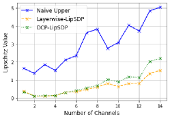
(a) Lipschitz estimations

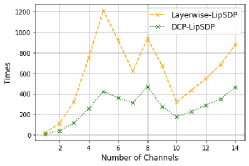
(b) solver times

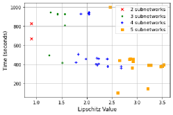
(c) subnetwork decompositions

Figure 1: Comparison of estimated Lipschitz constant  1(a) and solver time (seconds)  1(b) for varying channel size, as well as effects of the number and order of subnetworks  1(c).

We conduct experiments to demonstrate the effectiveness of DCP method used in tandem with the LipSDP-Neuron (Fazlyab et al., 2019) framework, which we refer to as DCP-LipSDP. We compare against the naive estimation $L=\prod_{i=1}^{l}\|\mathbf{W}_{i}\|_{2}$ (Szegedy et al., 2014), and the layer-wise acceleration method reviewed in Section 2, which we refer to as Layerwise-LipSDP. All experiments were implemented in Python. We used the CVXPY (Diamond & Boyd, 2016) toolbox and MOSEK (ApS, 2019) to formulate and solve the SDPs. All experiments used a 20-core CPU with 120GB of RAM. Base on this setup, we estimated $N_{\max}$ to be $1400$. All subsequent subnetworks resulting from DCP-LipSDP and Layerwise-LipSDP were constrained to be less than this value.

5.1 Performance Analysis

First, we evaluate the effectiveness of DCP-LipSDP to convolutional layers of increasing width, using toy networks with random weights from the Kaiming distribution (He et al., 2015). We constructed a convolutional block with an input size $10\times 10\times 1$ proceeded by $7$ convolutional layers, each with a filter size $2\times 2\times c$ and stride $1$, where $c$ is the number of output channels. We increased the width by varying $c$ from $1$ to $14$ and enforced that the number of subnetworks resulting from our method was the same as that from Layerwise-LipSDP, to highlight the effect of the proposed convolutional partitioning. A partition factor of $2$ was applied at each resulting subnetwork. The Lipschitz estimations and solve times are shown in Figure 1(a) and Figure 1(b) respectively. We observe that our method provides comparable Lipschitz estimations to Layerwise-LipSDP, andenhanced scalability evidenced by the reduced computation time. Specifically, we find an average reduction in solve time of $55\%$ from our method in comparison to Layerwise-LipSDP.

Following this, we examine larger CNNs trained on the MNIST (LeCun, 1998) and CIFAR-10 (Krizhevsky et al., 2009) datasets. CNN1 was trained on MNIST reaching a training accuracy of $99.7\%$, with a similar architecture to the CNN in Example 3 of (Gramlich et al., 2023). Specifically, CNN1 has an input size of $28\times 28\times 1$, followed by 2 convolutional layers each with a filter size of $5\times 5\times 5$ and stride 1, proceeded by a fully-connected layers of size 50. This corresponds to a network size of $784\rightarrow 2880\rightarrow 2000\rightarrow 50$ after being flattened. CNN2 was trained on CIFAR10, reaching a training accuracy of $70.6\%$. It has an input size of $32\times 32\times 3$ proceeded by 5 convolutional layers each with a filter size $2\times 2\times 5$ and stride 1, followed by 2 fully-connected layers of sizes $50,100$ and $100$. This corresponds to a network size of $3072\rightarrow 4500\rightarrow 3920\rightarrow 3380\rightarrow 2880\rightarrow 2420\rightarrow 50\rightarrow 100$, after being flattened. These networks were too large for LipSDP, so we compared to the naive estimation. The results are reported in Table 1. It can be seen that our method provides a tighter Lipschitz upper-bound than naive estimation in all cases, computed within a reasonable time. It is worth to mention that, after applying the DCP method, the largest problem size resulted from the subnetworks of CNN1 is 1304 while 1220 of CNN2. Therefore, the overall computing time of CNN2 is less, benefited from the parallel implementation, although it is actually a larger network.

Table 1: Lipschitz estimation and computing time for trained CNNs.

Neural Networks	Naive Estimation	DCP-LipSDP Estimation	DCP-LipSDP Time in Sec.
CNN1-MNIST	91.31	65.84	864
CNN2-CIFAR10	$3.73\times 10^{8}$	$1.48\times 10^{6}$	445

5.2 DCP Analysis

We perform further analysis for DCP using networks with random Kaiming weights.

Effect of Subnetwork Number and Order. It is theoretically possible that when applying Lemma 3.1, a tighter Lipschitz upper-bound can be obtained by considering fewer subnetworks. To analyse this phenomenon, we consider the model with 14 channels from Section 5.1 and vary both the number and order of subnetworks, characterised by the set $\mathcal{C}_{s}$. From Figure 1(c) we find that increasing the number of subnetworks $s$, from $2$ to $5$, can generally result in a more conservative Lipschitz upper-bound, thus a less accurate estimation. Changing the ordering for a given value of $s$ (indicated by different markers of the same colour in Figure 1(c)), in combination with the choice of the partition factor, affects the maximum size of the largest convolutional block, which in turn impacts the solver time.

Effect of Partition Factor. To examine the effects of the partition factor, we considered a $10$-layer convolutional block with an input size of $64\times 64\times 1$, filter size $5\times 5\times 1$ and stride $1$. This corresponds to an input dimension of $4096$, a maximum hidden-layer width of $3600$ and an output dimension of $576$ when flattened. The results in Figure 2(a) indicate a tighter Lipschitz upper bound for smaller values of $d$. All reported Lipschitz values were lower than the naive bound of $7.05$. Additionally, we considered a $2$-layer convolutional block with input $28\times 28\times 1$ and output $20\times 20\times 1$ to verify the order of the ratio of per-iteration time complexity as derived in Proposition 4.3. The results in Figure 2(b) show a decrease in complexity as the partition factor $d$ increases, suggesting the use of larger values of $d$ in the earlier layers where the output sizes tend to be larger, to improve scalability.

Effect of Chosen RIP Element. We examine how changing the choice of partition affects the accuracy and scalability. We considered a $2$-layer convolutional block with input $32\times 32\times 1$ and output $24\times 24\times 1$, i.e. $n_{\ell}=24$, for a fixed partition factor of $3$. We computed the RIP of $24$ into $3$-parts and selected 8 distinct partitions whereby the difference in size between the smallest and largest part is decreasing. Figure 2(c) indicates that, in this case, maximising the difference in size between the largest and smallest convolutional blocks, gives the tightest Lipschitz upper bound, but is the least scalable. Our current implementation sorts all partitions in lexicographical order, encouraging a larger size difference and a potentially more accurate estimation.

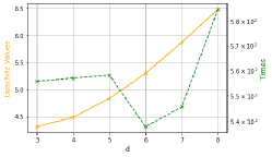
(a) Accuracy & scalability trade-off for increasing values of $d$.

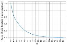
(b) Per-iteration acceleration for increasing values of $d$.

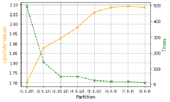
(c) Lipschitz estimations and solver time (seconds) for different $3$-part partitions.

Figure 2: Effects of the partition factor $d$ and chosen RIPs on accuracy and scalability.

6 Conclusion and Future Work

We have proposed a novel acceleration method to scale Lipschitz estimation to deep and wide CNNs. The DCP method incorporates a joint layer and width-wise partitioning, to decompose a large convolutional block into independent smaller blocks, permitting parallel implementation. We have proven a Lipschitz upper-bound in terms of the Lipschitz constants of the smaller blocks. We have demonstrated the effectiveness of the proposed method by experimenting with the LipSDP-Neuron framework, though our method is framework-invariant and can be used in conjunction with any estimation method. We have observed empirically that the reduction of the number of subnetworks, a smaller partition factor and increasing the size difference between the largest and smallest convolutional block, can result in a tighter Lipschitz upper-bound but is less scalable.

In general, solving (4.1.3) is a challenging problem due to the computational cost of evaluating the objective function as well as the identification and the size of the feasible set. Hitherto, we have relaxed it to a search problem, prioritising the constraint feasibility while weakly addressing the minimisation of the Lipschitz upper-bound through the lexicographical ordering of the RIPs. In the future, we will continue to research more effective ways to approximate and solve (4.1.3), and to address the accuracy-scalability trade-off. We will also attempt to provide theoretical guarantees of the tightness of the bound. Furthermore, we aim to explore the application of DCP to a wider range of network architectures. Of particular interest is the application to networks that encapsulate convolutional blocks, e.g. function compositions of the form: $g\circ\textmd{Conv}(\cdot)$. Through leveraging Lemma 3.1, DCP can be applied to accelerate the Lipschitz estimation for the convolutional block $\textmd{Conv}(\cdot)$, while the Lipschitz constant of $g$ can be estimated separately. Examples include architectures incorporating pooling layers (Pauli et al., 2023) and skip connections (Araujo et al., 2023), both formulated via SDP-based frameworks. So far we have achieved increased acceleration by exploiting network sparsity. In the future, we will investigate other acceleration strategies for scaling Lipschitz estimation to a wider range of network structures, such as self-attention (Kim et al., 2021) and equilibrium networks (Revay et al., 2020).

Appendix A Appendix

A.1 DCP Pseudocode

Algorithm 1 Dynamic Convolutional Partition (DCP)

1:Convolutional block $F:\mathbb{R}^{n_{0}\times n_{0}\times c_{0}}\to\mathbb{R}^{n_{\ell}\times n_{\ell}\times c_{\ell}}$. Empirically estimated $N_{\max}$.

2:Flattened subnetworks $\mathcal{F}=\left\{\left.\widetilde{f}_{ij}^{k}\right|i,j\in[d_{k}],k\in[s]\right\}$.

3:STOP $\leftarrow$ false, $s\leftarrow 0$, $\mathcal{C}_{s}\leftarrow\emptyset,D=\emptyset,R=\emptyset,\mathcal{F}\leftarrow\emptyset$;

4:while !STOP do

5:     $d\leftarrow 2$;

6:     Compute the set of $d$-part RIPs of $n_{\ell}$, as $\mathcal{P}_{d}\leftarrow R^{n_{\ell}}_{d}$

7:     for $r\in\mathcal{P}_{d}$ do

8:         Compute constraint dimensions for subnetwork indexed by $(\ell-2,\ell)$;

9:         if Eq. (19) is violated then

10:              $d\leftarrow d+1$, restart from 6;

11:         else

12:              $s\leftarrow s+1$, $d_{s}\leftarrow d,r_{s}\leftarrow r$;

13:              while $\ell\geq 1$ do

14:                  $L\leftarrow\ell$

15:                  Compute constraint dimensions for subnetwork indexed by $(L-1,\ell)$;

16:                  if Eq. (19) is not violated then

17:                       $L\leftarrow L-1$;

18:                  else

19:                       $C_{s}\leftarrow C_{s}\cup\{L,\ell\},D\leftarrow D\cup\{d_{s}\},R\leftarrow R\cup\{r_{s}\}$

20:                       $s\leftarrow s+1$, $\ell\leftarrow L$;

21:                       Restart from 5;

22:                  end if

23:              end while

24:              STOP $\leftarrow$ true;

25:         end if

26:     end for

27:end while

28:Return flattened subnetwork $\mathcal{F}$ using $C_{s},D\,\textrm{and}\,R$.

A.2 Proof of Theorem 4.1.

Focusing on the flattened, partitioned CNN $F_{u}$ as defined in Equation 11 and according to the definition of Lipschitz constant based on $l_{2}$-norm, for any two arbitrary inputs of $F_{u}$ denoted by $\mathbf{x}^{0}$ and $\mathbf{y}^{0}$, we have

$$\left\|F_{u}\left(\mathbf{x}^{0}\right)-F_{u}\left(\mathbf{y}^{0}\right)\right\|_{2}^{2}=\sum_{i,j=1}^{d}\left|\widetilde{f}_{ij}\left(\mathbf{x}_{ij}^{0}\right)-\widetilde{f}_{ij}\left(\mathbf{y}_{ij}^{0}\right)\right|^{2}\leq\sum_{i,j=1}^{d}L\left(\widetilde{f}_{ij}\right)\left\|\mathbf{x}_{ij}^{0}-\mathbf{y}_{ij}^{0}\right\|_{2}^{2}.$$ (22)

Defining the two vectors:

$$\boldsymbol{\gamma}\coloneqq \left[L\left(\widetilde{f}_{11}\right)^{2},L\left(\widetilde{f}_{12}\right)^{2},\ldots,L\left(\widetilde{f}_{dd}\right)^{2}\right]^{\top},$$

$$\underline{\Delta}\coloneqq \left[\|\mathbf{x}_{11}^{0}-\mathbf{y}_{11}^{0}\|_{2}^{2},\;\|\mathbf{x}_{12}^{0}-\mathbf{y}_{12}^{0}\|_{2}^{2},\ldots,\|\mathbf{x}_{dd}^{0}-\mathbf{y}_{dd}^{0}\|_{2}^{2}\right]^{\top},$$

and applying the Cauchy-Schwartz inequality, we obtain

$$\left\|F_{u}\left(\mathbf{x}^{0}\right)-F_{u}\left(\mathbf{y}^{0}\right)\right\|_{2}^{2}\leq\langle\boldsymbol{\gamma},\underline{\Delta}\rangle\leq\|\boldsymbol{\gamma}\|_{2}\|\underline{\Delta}\|_{2}.$$ (23)

Given

$$\|\underline{\Delta}\|_{2}^{2}=\sum_{i,j=1}^{d}\left\|\mathbf{x}_{ij}^{0}-\mathbf{y}_{ij}^{0}\right\|_{2}^{4},$$ (24)

we observe the following

$$\left\|\mathbf{x}^{0}-\mathbf{y}^{0}\right\|_{2}^{4}=\bigg{(}\sum_{i,j=1}^{d}\left\|\mathbf{x}_{ij}^{0}-\mathbf{y}_{ij}^{0}\right\|_{2}^{2}\bigg{)}^{2}=\sum_{i,j=1}^{d}\left\|\mathbf{x}_{ij}^{0}-\mathbf{y}_{ij}^{0}\right\|_{2}^{4}+\zeta=\|\underline{\Delta}\|_{2}^{2}+\zeta,$$ (25)

where $\zeta$ denotes all the additional non-negative terms from the expansion. This results in

$$\|\underline{\Delta}\|_{2}\leq\left\|\mathbf{x}^{0}-\mathbf{y}^{0}\right\|_{2}^{2}.$$ (26)

Combining (23) and (26), we have

$$\left\|F_{u}\left(\mathbf{x}^{0}\right)-F_{u}\left(\mathbf{y}^{0}\right)\right\|_{2}\leq\sqrt{\|\boldsymbol{\gamma}\|_{2}}\left\|\mathbf{x}^{0}-\mathbf{y}^{0}\right\|_{2}=\left(\sum_{i,j=1}^{d}L\left(\widetilde{f_{ij}}\right)^{4}\right)^{\frac{1}{4}}\left\|\mathbf{x}^{0}-\mathbf{y}^{0}\right\|_{2}.$$ (27)

We have shown that $L(F_{u})$ is bounded above by $\left(\sum_{i,j=1}^{d}L\left(\widetilde{f_{ij}}\right)^{4}\right)^{\frac{1}{4}}$, which concludes the proof.

A.3 Proof of Corollary 4.2

An $\ell$-layer convolutional block is a composite function of the $s$subnetworks, as detailed by (13) and (14). From Lemma 3.1, it follows that

$$L(F_{u})\leq\prod_{k=1}^{s}L(F_{k}^{u}).$$ (28)

Then apply Theorem 4.1 to bound the Lipschitz constant of each subnetwork $F_{k}^{u}$ by

$$L(F_{k}^{u})\leq\Biggl{(}\sum_{i,j=1}^{d_{k}}L\left(\widetilde{f}_{ij}^{(k)}\right)^{4}\Biggr{)}^{\frac{1}{4}}.$$ (29)

Substituting (29) into (28) gives the required result:

$$L(F_{u})\leq\prod_{k=1}^{s}L(F_{k}^{u})\leq\prod_{k=1}^{s}\Biggl{(}\sum_{i,j=1}^{d_{k}}L\left(\widetilde{f}_{ij}^{(k)}\right)^{4}\Biggr{)}^{\frac{1}{4}}.$$ (30)

A.4 Proof of Proposition 4.3.

For an $\ell$-layer convolutional block with a filter of dimension $h$ and stride $s$ applied at each convolutional layer, the formula for computing the output size is: $n_{k}=\lfloor\frac{n_{k-1}-h}{s}\rfloor+1$, i.e. $n_{k-1}=s(n_{k}-\epsilon_{k}-1)+h$, for $k\in\{1,2,\ldots,\ell\}$ and $\epsilon_{k}\in\{0,1\}$. The value of $\epsilon_{k}$ accounts for if $\lfloor\cdot\rfloor$ is a non-integer. From this the dimension of the $k$-th receptive field can be expressed in terms of $n_{\ell}$ as follows

$$n_{k}=s^{\ell-k}n_{\ell}+\sum_{i=1}^{\ell-k}(fs^{i-1}-s^{i}-\epsilon_{i}s^{i}),\,\textrm{for }\,k\in\{0,1,\ldots,\ell-1\}.$$ (31)

Similarly, the $k$-th receptive field corresponding to the largest convolutional block is given by

$$\rho_{k}=s^{\ell-k}\rho_{*}+\sum_{i=1}^{\ell-k}(fs^{i-1}-s^{i}-\epsilon_{i}s^{i}),\,\textrm{for }\,k\in\{0,1,\ldots,\ell-1\},$$ (32)

where we recall that $\rho_{*}$ denotes the dimension of of the largest convolutional block in the final layer, resulting from applying a $d$-part RIP to $n_{\ell}$.

To obtain (20) and (21), we state a few facts. First the number of equality constraints in (3.2) is one, i.e. $m=1$. Secondly, for deep networks the per-iteration time complexity is dominated by the cubic term. Using the fact that $N=\sum_{i=0}^{\ell-1}c_{i}n_{i}^{2}$ and $N_{*}=\sum_{i=0}^{\ell-1}c_{i}\rho_{i}^{2}$ for the largest convolutional block, substitution of (31) gives

$$N= \begin{multlined}c_{\ell-1}\Bigg{[}sn_{\ell}+\sum_{i=1}^{1}(fs^{i-1}-s^{i}-\epsilon_{i}s^{i})\Bigg{]}^{2}+c_{\ell-2}\Bigg{[}s^{2}n_{\ell}+\sum_{i=1}^{2}(fs^{i-1}-s^{i}-\epsilon_{i}s^{i})\Bigg{]}^{2}+\\ \ldots+c_{0}\Bigg{[}s^{\ell}n_{\ell}+\sum_{i=1}^{\ell}(fs^{i-1}-s^{i}-\epsilon_{i}s^{i})\Bigg{]}^{2}\end{multlined}c_{\ell-1}\Bigg{[}sn_{\ell}+\sum_{i=1}^{1}(fs^{i-1}-s^{i}-\epsilon_{i}s^{i})\Bigg{]}^{2}+c_{\ell-2}\Bigg{[}s^{2}n_{\ell}+\sum_{i=1}^{2}(fs^{i-1}-s^{i}-\epsilon_{i}s^{i})\Bigg{]}^{2}+\\ \ldots+c_{0}\Bigg{[}s^{\ell}n_{\ell}+\sum_{i=1}^{\ell}(fs^{i-1}-s^{i}-\epsilon_{i}s^{i})\Bigg{]}^{2}$$ (35)

$$= \begin{multlined}n_{\ell}^{2}\sum_{i=0}^{\ell-1}c_{i}s^{2(\ell-i)}+2n_{\ell}\Bigg{[}\sum_{j=1}^{\ell}c_{\ell-j}s^{j}\sum_{i=1}^{j}(fs^{i-1}-s^{i}-\epsilon_{i}s^{i})\Bigg{]}+\\ \sum_{j=1}^{\ell}c_{\ell-j}\Bigg{(}\sum_{i=1}^{j}(fs^{i-1}-s^{i}-\epsilon_{i}s^{i})\Bigg{)}^{2}.\end{multlined}n_{\ell}^{2}\sum_{i=0}^{\ell-1}c_{i}s^{2(\ell-i)}+2n_{\ell}\Bigg{[}\sum_{j=1}^{\ell}c_{\ell-j}s^{j}\sum_{i=1}^{j}(fs^{i-1}-s^{i}-\epsilon_{i}s^{i})\Bigg{]}+\\ \sum_{j=1}^{\ell}c_{\ell-j}\Bigg{(}\sum_{i=1}^{j}(fs^{i-1}-s^{i}-\epsilon_{i}s^{i})\Bigg{)}^{2}.$$ (38)

In an analogous way, we find $N_{*}$ to be

$$N_{*}=\rho_{*}^{2}\sum_{i=0}^{\ell-1}c_{i}s^{2(\ell-i)}+2\rho_{*}\Bigg{[}\sum_{j=1}^{\ell}c_{\ell-j}s^{j}\sum_{i=1}^{j}(fs^{i-1}-s^{i}-\epsilon_{i}s^{i})\Bigg{]}+$$

$$\sum_{j=1}^{\ell}c_{\ell-j}\Bigg{(}\sum_{i=1}^{j}(fs^{i-1}-s^{i}-\epsilon_{i}s^{i})\Bigg{)}^{2}.$$ (39)

To simplify the notation, let $a_{0},a_{1},a_{2}$ denote the first, second and third summation terms in (35) respectively- and likewise for (A.4). Then by considering the cubic binomial expansion of $N_{*}/N$, we obtain the following

$$\bigg{(}\frac{N_{*}}{N}\bigg{)}^{3}=\frac{a_{0}^{3}\rho_{*}^{6}+8a_{1}^{3}\rho_{*}^{3}+a_{2}^{3}+\zeta_{1}}{a_{0}^{3}n_{\ell}^{6}+8a_{1}^{3}n_{\ell}^{3}+a_{2}^{3}+\zeta_{2}},$$ (40)

where $\zeta_{1}$ and $\zeta_{2}$ denote lower order terms. Using the fact that there exist $b_{0},b_{1}>a_{0}$ such that $a_{0}^{3}n_{\ell}^{6}\leq N^{3}\leq b_{0}^{3}n_{\ell}^{6}$ and $a_{0}^{3}\rho_{*}^{6}\leq N_{*}^{3}\leq b_{1}^{3}\rho_{*}^{6}$, then (40) is bounded above as follows

$$\bigg{(}\frac{N_{*}}{N}\bigg{)}^{3}\leq\bigg{(}\frac{b_{1}}{a_{0}}\bigg{)}^{3}\bigg{(}\frac{\rho_{*}}{n_{\ell}}\bigg{)}^{6}.$$ (41)

To derive the results in (20) and (21) we use the fact that $\lceil\frac{n_{\ell}}{d}\rceil\leq\rho_{*}\leq n_{\ell}-(d-1)$ and consider the two following cases:

Case I. When $d=n_{\ell}$, $\rho_{*}$ can be at most 1. Substituting this value into (41) gives:

$$\bigg{(}\frac{N_{*}}{N}\bigg{)}^{3}\leq\bigg{(}\frac{b_{1}}{a_{0}}\bigg{)}^{3}\frac{1}{n_{\ell}^{6}}=O\bigg{(}\frac{1}{n_{\ell}^{6}}\bigg{)},\,\textrm{as}\,n_{\ell}\rightarrow\infty.$$ (42)

Case II. When $d=2$, $\rho_{*}$ can be at most $\lceil\frac{n_{\ell}}{2}\rceil$. Substituting this value into (41) gives:

$$\bigg{(}\frac{N_{*}}{N}\bigg{)}^{3}\leq\bigg{(}\frac{b_{1}}{a_{0}}\bigg{)}^{3}\frac{1}{2^{6}}=O(1).$$ (43)

A.5 Additional Information and Experiments

A.5.1 $N_{\max}$ Estimation

The estimation of $N_{\max}$ involves generating multiple SDPs of increasing size and recording the constraint size for which computational bottlenecks. Averaging over these instances will give an estimation for $N_{\max}$. While this approximation will be tight, it is not cheap to compute it as the problem size for which bottlenecks are reached, is not known a priori, even though this can be accelerated by parallel implementation.

As an alternative, we implement a prediction-based method, which may give a more conservative estimate of $N_{\max}$ but is computationally cheaper. It runs LipSDP on several small to medium sized problems, recording the memory usage. Using the collected data, $N_{\max}$ is estimated via extrapolation. While this still involves multiple calls of LipSDP, it avoids having to increment the problem size until computational bottlenecks, which isn’t known a priori, and is thus is more efficient. In Figure 3, we show the recorded memory usage of the solver for increasing problem sizes (y_true) and compared against a quadratic fit of the data (y_poly). Using the approximating polynomial, we extrapolated the value of $N_{\max}$ based on a maximum memory capacity of $120$GB of RAM, which gave a value of $1800$. We chose a more conservative value than this in practice, i.e., $N_{\max}=1400$, to account for memory associated with additional computations and running the operating system.

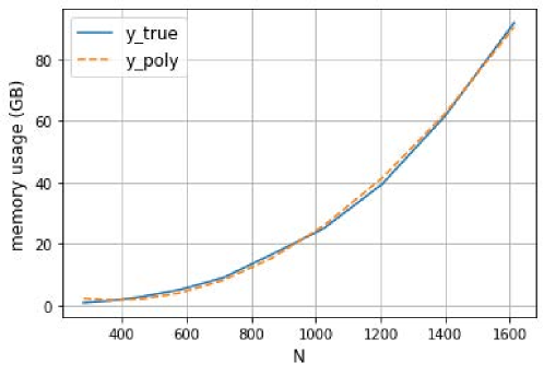
Figure 3: Memory usage for increasing problem dimensions.

A.5.2 Provably 1-Lipschitz Network

To further assess the effectiveness of the DCP method, we apply it to provably 1-Lipschitz networks. As mentioned in (Anil et al., 2019), a provably 1-Lipschitz network is one which is composed of 1-Lipschitz affine transformations and activations. To this end, we consider a 2-layer convolutional block with an input dimension of $28\times 28$, followed by two convolutional layers of sizes $12\times 12\times c$ and $4\times 4\times 1$, where the number of channels, c, varies from 1 to 3. We used the ReLU activation function that is 1-Lipschitz, and orthogonalised the weight matrices. The results are shown in Table 2. The LipSDP estimations are less than 1, which we conjecture is due to the approximation error underpinning the SDP formulation. As expected, DCP-LipSDP returns estimations greater than the LipSDP ones, being their upper-bounds.

Table 2: Comparison of Lipschitz estimation for provably 1-Lipschitz, 2-layer convolutional blocks of size $28\times 28\rightarrow 12\times 12\times c\rightarrow 4\times 4$.

Channel Number ($c$)	LipSDP	DCP-LipSDP
1	0.85	1.03
2	0.63	0.79
3	0.64	0.82

References

- Açıkmeşe & Corless (2011) Behçet Açıkmeşe and Martin Corless. Observers for systems with nonlinearities satisfying incremental quadratic constraints. Automatica, 47(7):1339–1348, 2011.
- Agler et al. (1988) Jim Agler, William Helton, Scott McCullough, and Leiba Rodman. Positive semidefinite matrices with a given sparsity pattern. Linear algebra and its applications, 107:101–149, 1988.
- Akhtar & Mian (2018) Naveed Akhtar and Ajmal Mian. Threat of adversarial attacks on deep learning in computer vision: A survey. Ieee Access, 6:14410–14430, 2018.
- Andrews & Eriksson (2004) George E Andrews and Kimmo Eriksson. Integer partitions. Cambridge University Press, 2004.
- Anil et al. (2019) Cem Anil, James Lucas, and Roger Grosse. Sorting out lipschitz function approximation. In International Conference on Machine Learning, pp. 291–301. PMLR, 2019.
- ApS (2019) Mosek ApS. Mosek optimization toolbox for matlab. User’s Guide and Reference Manual, Version, 4, 2019.
- Araujo et al. (2023) Alexandre Araujo, Aaron J Havens, Blaise Delattre, Alexandre Allauzen, and Bin Hu. A unified algebraic perspective on lipschitz neural networks. In The Eleventh International Conference on Learning Representations, 2023.
- Bojarski et al. (2016) Mariusz Bojarski, Davide Del Testa, Daniel Dworakowski, Bernhard Firner, Beat Flepp, Prasoon Goyal, Lawrence D Jackel, Mathew Monfort, Urs Muller, Jiakai Zhang, et al. End to end learning for self-driving cars. arXiv preprint arXiv:1604.07316, 2016.
- Cobzaş et al. (2019) Ştefan Cobzaş, Radu Miculescu, and Adriana Nicolae. Lipschitz functions, volume 10. Springer, 2019.
- Combettes & Pesquet (2020) Patrick L Combettes and Jean-Christophe Pesquet. Lipschitz certificates for layered network structures driven by averaged activation operators. SIAM Journal on Mathematics of Data Science, 2(2):529–557, 2020.
- Diamond & Boyd (2016) Steven Diamond and Stephen Boyd. CVXPY: A Python-embedded modeling language for convex optimization. Journal of Machine Learning Research, 17(83):1–5, 2016.
- Eger (2013) Steffen Eger. Restricted weighted integer compositions and extended binomial coefficients. J. Integer Seq, 16(13.1):3, 2013.
- Esteva et al. (2017) Andre Esteva, Brett Kuprel, Roberto A Novoa, Justin Ko, Susan M Swetter, Helen M Blau, and Sebastian Thrun. Dermatologist-level classification of skin cancer with deep neural networks. nature, 542(7639):115–118, 2017.
- Fazlyab et al. (2019) Mahyar Fazlyab, Alexander Robey, Hamed Hassani, Manfred Morari, and George Pappas. Efficient and accurate estimation of lipschitz constants for deep neural networks. Advances in Neural Information Processing Systems, 32:11427–11438, 2019.
- Fukuda et al. (2001) Mituhiro Fukuda, Masakazu Kojima, Kazuo Murota, and Kazuhide Nakata. Exploiting sparsity in semidefinite programming via matrix completion i: General framework. SIAM Journal on optimization, 11(3):647–674, 2001.
- Garstka et al. (2020) Michael Garstka, Mark Cannon, and Paul Goulart. A clique graph based merging strategy for decomposable sdps. IFAC-PapersOnLine, 53(2):7355–7361, 2020.
- Goodfellow et al. (2014) Ian J Goodfellow, Jonathon Shlens, and Christian Szegedy. Explaining and harnessing adversarial examples. arXiv preprint arXiv:1412.6572, 2014.
- Gramlich et al. (2023) Dennis Gramlich, Patricia Pauli, Carsten W Scherer, Frank Allgöwer, and Christian Ebenbauer. Convolutional neural networks as 2-d systems. arXiv preprint arXiv:2303.03042, 2023.
- He et al. (2015) Kaiming He, Xiangyu Zhang, Shaoqing Ren, and Jian Sun. Delving deep into rectifiers: Surpassing human-level performance on imagenet classification. In Proceedings of the IEEE international conference on computer vision, pp. 1026–1034, 2015.
- Heubach & Mansour (2004) Silvia Heubach and Toufik Mansour. Compositions of n with parts in a set. Congressus Numerantium, 168:127, 2004.
- Kim et al. (2021) Hyunjik Kim, George Papamakarios, and Andriy Mnih. The lipschitz constant of self-attention. In International Conference on Machine Learning, pp. 5562–5571. PMLR, 2021.
- Krizhevsky et al. (2009) Alex Krizhevsky, Geoffrey Hinton, et al. Learning multiple layers of features from tiny images. 2009.
- Latorre et al. (2019) Fabian Latorre, Paul Rolland, and Volkan Cevher. Lipschitz constant estimation of neural networks via sparse polynomial optimization. In International Conference on Learning Representations, 2019.
- LeCun (1998) Yann LeCun. The mnist database of handwritten digits. http://yann. lecun. com/exdb/mnist/, 1998.
- Madry et al. (2018) Aleksander Madry, Aleksandar Makelov, Ludwig Schmidt, Dimitris Tsipras, and Adrian Vladu. Towards deep learning models resistant to adversarial attacks. In International Conference on Learning Representations, 2018.
- Majumdar et al. (2020) Anirudha Majumdar, Georgina Hall, and Amir Ali Ahmadi. Recent scalability improvements for semidefinite programming with applications in machine learning, control, and robotics. Annual Review of Control, Robotics, and Autonomous Systems, 3:331–360, 2020.
- Opdyke (2010) John Douglas Opdyke. A unified approach to algorithms generating unrestricted and restricted integer compositions and integer partitions. Journal of Mathematical Modelling and Algorithms, 9(1):53–97, 2010.
- Pauli et al. (2021) Patricia Pauli, Anne Koch, Julian Berberich, Paul Kohler, and Frank Allgöwer. Training robust neural networks using lipschitz bounds. IEEE Control Systems Letters, 6:121–126, 2021.
- Pauli et al. (2023) Patricia Pauli, Dennis Gramlich, and Frank Allgöwer. Lipschitz constant estimation for 1d convolutional neural networks. In Learning for Dynamics and Control Conference, pp. 1321–1332. PMLR, 2023.
- Raghunathan et al. (2018) Aditi Raghunathan, Jacob Steinhardt, and Percy Liang. Certified defenses against adversarial examples. In International Conference on Learning Representations, 2018.
- Revay et al. (2020) Max Revay, Ruigang Wang, and Ian R Manchester. Lipschitz bounded equilibrium networks. arXiv preprint arXiv:2010.01732, 2020.
- Scaman & Virmaux (2018) Kevin Scaman and Aladin Virmaux. Lipschitz regularity of deep neural networks: analysis and efficient estimation. In Proceedings of the 32nd International Conference on Neural Information Processing Systems, pp. 3839–3848, 2018.
- Sedghi et al. (2018) Hanie Sedghi, Vineet Gupta, and Philip M Long. The singular values of convolutional layers. In International Conference on Learning Representations, 2018.
- Singla & Feizi (2021) S Singla and S Feizi. Fantastic four: Differentiable bounds on singular values of convolution layers. In International Conference on Learning Representations (ICLR), 2021.
- Szegedy et al. (2014) Christian Szegedy, Wojciech Zaremba, Ilya Sutskever, Joan Bruna, Dumitru Erhan, Ian Goodfellow, and Rob Fergus. Intriguing properties of neural networks. In International Conference on Learning Representations, 2014. URL http://arxiv.org/abs/1312.6199.
- Vajnovszki (2013) Vincent Vajnovszki. Generating permutations with a given major index. arXiv preprint arXiv:1302.6558, 2013.
- Vandenberghe & Boyd (1996) Lieven Vandenberghe and Stephen Boyd. Semidefinite programming. SIAM review, 38(1):49–95, 1996.
- Vandenberghe et al. (2015) Lieven Vandenberghe, Martin S Andersen, et al. Chordal graphs and semidefinite optimization. Foundations and Trends® in Optimization, 1(4):241–433, 2015.
- Xue et al. (2022) Anton Xue, Lars Lindemann, Alexander Robey, Hamed Hassani, George J Pappas, and Rajeev Alur. Chordal sparsity for lipschitz constant estimation of deep neural networks. In 2022 IEEE 61st Conference on Decision and Control (CDC), pp. 3389–3396. IEEE, 2022.
- Zheng et al. (2021) Yang Zheng, Giovanni Fantuzzi, and Antonis Papachristodoulou. Chordal and factor-width decompositions for scalable semidefinite and polynomial optimization. Annual Reviews in Control, 52:243–279, 2021.