Cavity Detection of Gravitational Waves: Where Do We Stand?

Abstract

High frequency gravitational waves (HFGWs) are predicted in various exotic scenarios involving both cosmological and astrophysical sources. These elusive signals have recently sparked the interest of a diverse community of researchers, due to the possibility of HFGW detection in the laboratory through graviton-photon conversion in strong magnetic fields. Notable examples include the redesign of the resonant cavities currently under development to detect the cosmic axion. In this work, we derive the sensitivities of some existing and planned resonant cavities to detect a HFGW background. As a concrete scenario, we consider the collective signals that originate from the merging of compact objects, such as two primordial black holes (PBHs) in the asteroid mass window. Our findings improve over existing work by explicitly discussing and quantifying the loss in the experimental reach due to the actual coherence of the source. We elucidate on the approach we adopt in relation with recent literature on the topic. Most notably, we give a recipe for the estimate of the stochastic background that focuses on the presence of the signal in the cavity at all times and showing that, in the relevant PBH mass region, the signal is dominated by coherent binary mergers.

I Introduction

The detection of gravitational waves (GWs) from compact mergers, made possible via a network of ground-based interferometers, has marked the dawn of GW astronomy Abbott et al. (2016, 2019). At present, these efforts focus on the sub-kHz GW frequency band, corresponding to the range in reach of the Laser Interferometer Gravitational-Wave Observatory, the Virgo interferometer, and the Kamioka Gravitational Wave Detector.

Nevertheless, the GW spectrum is expected to extend over various decades in frequencies. In fact, the detection in the nHz region of a GW background (GWB) has been recently confirmed by several consortia operating at the global scale, through pulsar timing array techniques McLaughlin (2013); Goncharov et al. (2021); Lee (2016); Chen et al. (2021). Moreover, the cosmic microwave background (CMB) provides with an indirect constrains on the primordial GWB spectrum at frequencies below the pHz Ade et al. (2015, 2018); Namikawa et al. (2019).

Near-future experiments plan to scan different bands encompassing different methods including the forthcoming ground-based Punturo et al. (2010); Hild et al. (2011) and space-based Amaro-Seoane et al. (2017); Yagi and Seto (2011) laser interferometers, atom interferometers Badurina et al. (2020); El-Neaj et al. (2020); Abe et al. (2021), and probes of the CMB Namikawa et al. (2019); Abazajian et al. (2022). These endeavors cover the GW bands at the kHz frequency and below, where astrophysical and cosmological sources from the merger of known compact objects are expected to provide with a GWB besides other possible sources of unknown origin.

A parallel search can be designed to involve high frequency gravitational waves (HFGWs), spanning frequency ranges well above the kHz. A GWB at high frequencies could potentially be sourced by a collection of exotic physical phenomena originating both in the early and late Universe. Examples include the merging of primordial black holes (PBHs) Dolgov and Ejlli (2011); Fujita et al. (2014); Herman et al. (2021); Gehrman et al. (2023); Franciolini et al. (2022); Banerjee and Dey (2023) or boson stars Liebling and Palenzuela (2023); Visinelli (2021), black hole (BH) superradiance Arvanitaki and Dubovsky (2011), models of modified gravity Jung et al. (2020); Lambiase et al. (2023), the primordial thermal plasma Ringwald et al. (2021), phase transitions in the early Universe Caprini et al. (2016); Caprini and Figueroa (2018); Addazi et al. (2024), the “slingshot” mechanism, taking place upon the coexistence of confined and unconfined vacua in the presence of heavy quarks Bachmaier et al. (2023), a network of cosmic strings Kibble (1976); Vilenkin (1981, 1985); Witten (1985); Servant and Simakachorn (2023), post-inflation (p)reheating Figueroa and Torrenti (2017); Adshead et al. (2018), and inflationary mechanisms Kim et al. (2005); Vagnozzi and Loeb (2022).

A novel avenue for detecting GWs at such high frequencies in the GW spectrum has gained momentum in recent years, with various proposal being explored including interferometers Cruise and Ingley (2006); Akutsu et al. (2008); Nishizawa et al. (2008); Ackley et al. (2020), microwave and optical cavities Pegoraro et al. (1978); Caves (1979); Reece et al. (1984); Ballantini et al. (2003); Mensky and Rudenko (2009); Navarro et al. (2023), mechanical resonators Aguiar (2011); Goryachev et al. (2014), and superconducting rings Anandan and Chiao (1982). Insightful reviews are found in Refs. Aggarwal et al. (2021); Schmieden and Schott (2024).

One promising line that has recently been proposed involves the conversion of gravitons into photons via the inverse Gertsenshtein effect Gertsenshtein (1962); Zel’dovich (1973); Palessandro and Rothman (2023). This intriguing concept has positioned resonant cavities as promising candidates for detecting gravitational wave signals within the MHz-GHz HFGW band Aggarwal et al. (2021). Previous experiments such as Explorer at CERN, Nautilus at INFN-LNF, and Auriga at Legnaro predominantly targeted gravitational waves in the kHz range, emanating from the mergers of compact objects or comprising a GWB Astone et al. (1993, 1997). Cavity experiments extend the detection capability to higher frequencies, potentially spanning the range (0.1-10) GHz. This groundbreaking approach not only widens the spectrum of detectable gravitational waves but also paves the way for exploring phenomena such as the existence and distribution of PBHs within this yet uncharted frequency domain.

Various cavity searches are currently undergoing or planned to be operational in coming years, including the Axion Dark Matter eXperiment (ADMX)-G2 Du et al. (2018); Braine et al. (2020); Bartram et al. (2021), ADMX EFR Chakrabarty et al. (2024), the The Haloscope At Yale Sensitive To Axion CDM (HAYSTACK) Brubaker (2017), the FINUDA magnet for Light Axion SearcH (FLASH) Alesini et al. (2019, 2023), the International Axion Observatory (IAXO) in its intermediate stage BabyIAXO Abeln et al. (2021); Ahyoune et al. (2023), and the Axion Longitudinal Plasma HAloscope (ALPHA) Lawson et al. (2019); Millar et al. (2023). A proposed network of cavities that employs “quantum squeezing” would lower the noise and boost the efficiency of the search Backes et al. (2021); Brady et al. (2022). These endeavors collectively represent a concerted effort to advance our understanding of high-frequency gravitational waves and their potential implications in fundamental physics and cosmology.

In this work, we derive the sensitivities for the planned cavities in the case of the detection of both a GW signals and the corresponding GW background. As a practical example, we consider the GW signal released from BH mergers. This system is characterized by its potentially fast frequency swiping which, contrary to the axion case, can lead to a significant loss of the cavity reach Domcke et al. (2022); Franciolini et al. (2022). Our goal is to quantify explicitly such a suppression, detailing the procedures outlined in a previous experimental report Alesini et al. (2023).

While our approaches may seem straightforward, we believe this to be worth explicitly commenting on, given the above mentioned advancement and the excitement in the realm of HFGWs. As it turns out, the actual reach given by physical sources such as PBHs mergers is significantly worse than what previously discussed in the literature. Even in the best case scenario, the discrepancy between current experimental reaches and the physical GW signal amounts to about eight orders of magnitudes, for the case of BH mergers. Rather than interpreting our results as a negative outcome for the detection of HFGWs, we envision them as a catalyst for inspiring novel experimental setups and the study of GW sources.

Our paper is organized as follows. In Sec. II we outline the details of the expression used in the analyses. The results of our approach are presented in Sec. III and a discussion is developed in Sec. IV. Conclusions are drawn in Sec. V. Throughout the paper, we adopt the convention $\displaystyle\hbar=c=1$ unless otherwise stated.

II Method

II.1 Sensitivity forecast

The coupling of the photon with gravity is described by the Maxwell-Einstein action,

$$S=\int{\rm d}^{4}x\sqrt{-g}\left(-\frac{1}{4}g_{\mu\alpha}g_{\nu\beta}F^{\mu\nu}F^{\alpha\beta}\right)\,,$$ (1)

where $\displaystyle g_{\mu\nu}$ is the space-time metric with determinant $\displaystyle g$ and $\displaystyle F^{\mu\nu}$ is the electromagnetic field strength.

The term in Eq. (1) modifies the usual expressions of electrodynamics by introducing a new source, see Eq. (22) in Appendix A, and leads to a deposition of energy in the resonant cavity. To see this, the metric tensor is expanded to first order around a flat background as

$$g^{\mu\nu}=\eta^{\mu\nu}+h^{\mu\nu}\,,$$ (2)

where $\displaystyle|h^{\mu\nu}|\ll 1$ describes the perturbations. The action in Eq. (1) predicts a coupling between the GW signal and the electromagnetic (EM) energy tensor $\displaystyle T^{\mu\nu}_{\rm EM}$ with the Lagrangian $\displaystyle\mathcal{L}=(1/2)h_{\mu\nu}T^{\mu\nu}_{\rm EM}$. This leads to the effective coupling $\displaystyle\mathcal{L}\propto h_{0}B_{0}\delta B_{z}$ for a GW strain $\displaystyle h_{0}$ in an external magnetic field $\displaystyle B_{0}\hat{\bf z}$, where the magnetic field variation coupled within the cavity $\displaystyle\delta B_{z}$ can be picked up with a magnetometer.

To address the detection of a GW source by a resonating cavity we follow the discussion in Ref. Allen and Romano (1999), adapting the treatment originally expressed in terms of the search through interferometers to the case of a haloscope. Given the energy stored in the cavity $\displaystyle U$, the signal-to-noise ratio (SNR) is obtained as

$${\rm SNR}=\frac{2\pi U}{T_{\rm sys}}\,\sqrt{\Delta t\,\Delta f}\,,$$ (3)

where $\displaystyle T_{\rm sys}$ is the coldest effective temperature of the instrumentation and noise amplifier, $\displaystyle\Delta f$ is the frequency bandwidth, and $\displaystyle\Delta t$ is the time under which the signal is collected. The expression for the energy stored in the cavity is detailed in Eq. (41).

To begin with, we assume that we observe a sufficiently stationary source of GWs for a number of cycles $\displaystyle N_{\rm cycles}\gtrsim 1$. The source emits within the cavity frequency bandwidth $\displaystyle\Delta f=f/Q$, where $\displaystyle Q$ is the quality factor of the cavity, so that the reach of the strain $\displaystyle h_{0}$ is obtained by setting $\displaystyle{\rm SNR}=1$. Once the expression for the power of the signal in Eq. (45) is considered, this leads to an estimate for the strain at resonance as

$$\begin{split}h_{0}&\approx 6.0\times 10^{-23}\,\left(\frac{\rm 1\,T}{B_{0}}\right)\,\left(\frac{0.14}{\eta}\right)\,\left(\frac{\rm m^{3}}{V}\right)^{5/6}\,\left(\frac{10^{6}}{Q_{\rm eff}}\right)^{1/2}\\ &\times\left(\frac{T_{\rm sys}}{\rm K}\right)^{1/2}\,\left(\frac{\Delta f}{\rm kHz}\,\frac{\rm 1\,min}{t_{\rm eff}^{\rm int}}\right)^{1/4}\,\left(\frac{\rm GHz}{\omega_{n}/2\pi}\right)^{3/2}\,,\end{split}$$ (4)

where $\displaystyle Q_{\rm eff}={\rm min}(N_{\rm cycles},Q)$ is the effective quality factor, $\displaystyle\eta$ the coupling of the cavity with the gravitational signal defined in Eq. (42), $\displaystyle V$ the effective volume of the cavity, $\displaystyle T_{\rm sys}$ the system temperature, $\displaystyle\omega_{n}=2\pi f$ the resonant pulsation, and $\displaystyle t_{\rm eff}^{\rm int}={\rm min}(N_{\rm cycles}\,\omega_{n}^{-1},\Delta t)$ the minimum value between the experimental integration time and the source duration. For a detailed derivation and definition of all the above quantities we refer the reader to Appendix A.

The expression in Eq. (3) can also be used to estimate the sensitivity over a stochastic GW background. A GWB spectrum is generally assumed to be nearly isotropic, unpolarized, stationary, and characterized by a Gaussian distribution with zero mean. The fractional contribution to the density parameter $\displaystyle\Omega_{\rm GW}$ can be alternatively expressed in terms of a dimensionless characteristic strain $\displaystyle h_{c}$ as Thrane and Romano (2013); Romano and Cornish (2017)

$$\Omega_{\rm GW}(f)=\frac{(2\pi)^{2}}{3H_{0}^{2}}\,f^{2}\,h_{c}^{2}\,,$$ (5)

where $\displaystyle H_{0}$ is the Hubble constant.

As we discuss in Appendix A, provided $\displaystyle Q_{\rm eff}\sim Q$ - whose validity depends on the properties of the sources discussed below - the characteristic strain reach reads

$$\begin{split}h_{c}&\approx 6.0\times 10^{-20}\,\left(\frac{\rm 1\,T}{B_{0}}\right)\,\left(\frac{0.14}{\eta}\right)\,\left(\frac{\rm m^{3}}{V}\right)^{5/6}\\ &\times\left(\frac{T_{\rm sys}}{\rm K}\right)^{1/2}\,\left(\frac{\Delta f}{\rm kHz}\,\frac{\rm 1\,min}{t_{\rm obs}}\right)^{1/4}\,\left(\frac{\rm GHz}{\omega_{n}/2\pi}\right)^{3/2},\end{split}$$ (6)

where the total observation time of the experiment $\displaystyle t_{\rm obs}$ can strategically largely exceed the value chosen for the search for a coherent source.

So far, we have discussed the response of the cavity to a stationary signal. We now briefly comment on the coherence of the source. For the dark matter axion, the quality of the source is limited by thermal and quantum fluctuations which impact over the maximal capacity of the cavity to resonate with the signal. For the case of a GW signal from PBH mergers or other sources of HFGWs, the actual coherence of the GW signal at a given frequency is granted by the large number of gravitons in the parameter space of interest. This implies that the same approach as for the axion can be used to parametrize the non-stationarity of a HFGW source.

In fact, we can describe the gravitational wave signal as a coherent state of highly occupied gravitons of energy $\displaystyle\omega$, with the occupation number $\displaystyle N_{g}\sim\rho/\omega^{4}\sim m_{\rm Pl}^{2}h_{0}^{2}\,/\omega^{2}$ corresponding to the number of gravitons per de Broglie volume $\displaystyle\omega^{-3}$. Here, we have used the fact that the energy density of the GW signal is given by $\displaystyle\rho\sim h_{0}^{2}\omega^{2}m_{\rm Pl}^{2}$. For a coherent signal, typical fluctuations are of the order of $\displaystyle\delta N_{g}\sim\sqrt{N_{g}}$, leading to a quality of the signal $\displaystyle Q_{h}=N_{g}/\delta N_{g}\sim\sqrt{N_{g}}$. This quality factor is potentially degrading the quality of the source when it is smaller than the quality of the cavity $\displaystyle Q$. Therefore, the quality of the source is determined by the quantum origin of the signal.

For example, consider a GW signal with the frequency $\displaystyle f\sim 0.1$ GHz and a typical physical strain of the reach $\displaystyle h_{0}\sim 10^{-22}$, corresponding to the typical current reach of the cavity given in Eq. (11) below. In this setup, the number of gravitons is $\displaystyle N_{\rm g}\sim 10^{32}$, which implies a source quality $\displaystyle Q_{h}\sim 10^{16}$ that is much larger than the quality factor of the cavity. Even in the desirable scenario where the cavity would reach a sensitivity comparable to the actual physical signal of strain $\displaystyle h_{0}\sim 10^{-30}$, the source would possess the quality $\displaystyle Q_{h}\sim 10^{6}\gtrsim Q$. The consideration above therefore justifies the dropping of such a contribution from the treatment. Note, however, that if the sensitivity of the experiment could reach an even smaller sensitivity for this range of frequencies, part of the signal could be degraded.

II.2 Gravitational wave sources

Potential sources of GWs are generally divided into two categories, namely sources of cosmological origin produced before recombination and sources of astrophysical origin. A cosmological GWB at high frequencies, expected from exotic sources, can be constrained by BBN considerations and CMB data as Caprini and Figueroa (2018)

$$\Omega_{\rm GW}h_{H}^{2}\lesssim 5.6\times 10^{-6}\,\Delta N_{\rm eff}\,,$$ (7)

where $\displaystyle h_{H}=H_{0}/(100{\rm\,km\,s^{-1}\,Mpc^{-1}})$ is the reduced Hubble constant. The excess in the number of relativistic active neutrinos is constrained as $\displaystyle\Delta N_{\rm eff}\lesssim 0.3$ by various considerations on big-bang nucleosynthesis (BBN) in combinations with CMB data. Using Eq. (5), the bound above reads Domcke et al. (2022, 2024)

$$h_{c}\lesssim 2\times 10^{-30}\,\left({\rm GHz}/f\right)\,\Delta N_{\rm eff}^{1/2}\,,$$ (8)

which is several orders of magnitude below the expected reach of resonant cavities expressed in Eq. (6). Therefore, a potential detection of HFGWs can only be due to astrophysical sources in the late Universe.

However, since there are no known astrophysical sources releasing GWs at such high frequencies, new physics is likely required to motivate the search in the HFGW band. Possibilities include the decay of an unstable axion star after a binary merging Chung-Jukko et al. (2024) and the stimulated decay of dark matter (DM) in theories of Chern-Simons gravity Jung et al. (2020). We comment below on the merging of compact objects, with particular focus on the case of PBHs. We consider BHs that are too light to be explained by known stellar dynamics, so that their indirect detection through mergers would require new physics to explain their origins. A possibility is that these PBHs form in the early Universe, hence the name primordial. The exact details of the formation scenario are currently unknown. For example, they could result from inflationary overdensities Carr et al. (2021), from the collapse of bubbles in supercooled phase transitions Gouttenoire and Volansky (2023); Flores et al. (2024), from the confinement of heavy quarks Dvali et al. (2021), or many other methods Carr et al. (2021).

In Table 1 we report the main setups of some experiments that employ a resonant cavity, see the caption for the specific references. For each experiment, the noise temperature $\displaystyle T_{\rm sys}$ is obtained through the formula $\displaystyle T_{\rm sys}=\omega_{c}[1/(\exp(\omega_{c}/T_{\rm phys})-1)+N_{A}+0.5]$, where $\displaystyle\omega_{c}/(2\pi)$ is the central frequency in the band covered by the experiment and the number of states is $\displaystyle N_{A}=1/2$ everywhere except for FLASH and BabyIAXO, for which $\displaystyle N_{A}=10$. In this context, “FLASH HighT” refers to the initial phase of the experiment Alesini et al. (2023). This phase will undergo an upgrade with an enhanced cryostat to achieve the performance levels of “FLASH LowT”, which serve as benchmarks for the results discussed below.

Experiment	ADMX-G2	ADMX EFR	FLASH HighT	FLASH LowT	ALPHA	HAYSTACK	BabyIAXO
Frequency range [GHz]	0.6–2	2-4	0.117-0.206	0.117-0.206	5-40	4-6	0.253-0.469
Volume [m3]	0.085	0.080	4.156	4.156	0.334	0.0015	7.7
Unloaded $\displaystyle Q$/103	60	90	570–450	570–450	10	30	320
$\displaystyle B_{0}$  [T]	7.7	9.6	1.1	1.1	13	9	2
$\displaystyle T_{\rm phys}$  [K]	0.15	0.15	4.9	0.30	5.0	0.13	4.9
$\displaystyle T_{\rm sys}$  [K]	0.18	0.23	5.0	0.40	5.0	0.28	4.9

Table 1: Parameters defining the resonant cavity experiments considered in this work. Specifically, ADMX-G2 Du et al. (2018); Braine et al. (2020); Bartram et al. (2021), ADMX EFR Oblath (2023), FLASH low-frequency (LF) and high-frequency (HF) Alesini et al. (2023), ALPHA Lawson et al. (2019); Millar et al. (2023), HAYSTACK Brubaker (2017), and BabyIAXO Abeln et al. (2021); Ahyoune et al. (2023).

A fundamental question arises regarding whether these objects, regardless of how they formed, can constitute a substantial portion of DM. Cavity searches are sensitive to mergers involving sub-solar PBHs with masses ranging below about $\displaystyle 10^{-8}\,M_{\odot}$. This result, as we outline below, derives from requiring that at least one complete revolution of the binary system appears in the cavity tuned at the frequency around the GHz. This PBH mass range partially overlaps with the region of masses heavier than $\displaystyle 10^{-11}\,M_{\odot}$, in which stringent lensing constraints have already discounted PBHs as the primary constituents of DM Niikura et al. (2019). To sum up, in the region of masses $\displaystyle[10^{-11}\textrm{-}10^{-8}]\,M_{\odot}$ a minor contribution from PBHs to the DM abundance is still plausible Carr et al. (2021), while the region of masses below $\displaystyle 10^{-11}\,M_{\odot}$ is not currently constrained by microlensing results.

Although cavity experiments do not reach the sensitivity required to probe the type of signal from these sources, several uncertainties in cosmological history could substantially amplify the signal. One explicit possibility under discussion is the incorporation of significant non-Gaussianity from the inflationary period, which, in turn, could lead to an escalation in the merger rate Franciolini et al. (2022). Note, that even in the best scenario a maximal increase of about two orders of magnitude is feasible in the merger rate Franciolini et al. (2022).

Compact objects such as BH and neutron stars (NS) form in astrophysical environment. Possible and more exotic configurations such as PBHs or boson stars could have already been present in the earliest stages of the Universe Liebling and Palenzuela (2023); Visinelli (2021). Binaries of compact objects could fall in the frequency range and with a GW strain that is sufficiently strong to be detectable with present or near-future technologies. Consider two compact objects of similar mass $\displaystyle M$ and size $\displaystyle R$, and each of compactness $\displaystyle\mathrm{C}\equiv GM/R$, forming a system of total mass $\displaystyle M_{\rm TOT}\approx 2M$. The frequency of the emitted GW spectrum at the end of the inspiral phase, when the stars occupy the innermost stable circular orbit, is Giudice et al. (2016)

$$f=\frac{\mathrm{C}^{3/2}}{3\sqrt{3}\pi GM_{\rm TOT}}\,.$$ (9)

For example, a signal in the bandwidth $\displaystyle\mathcal{O}(100\,{\rm MHz})$ gives

$$M_{\rm TOT}\approx 4\times 10^{-6}\,M_{\odot}\,\left(\frac{\mathrm{C}}{0.1}\right)^{3/2}\,,$$ (10)

which, for the compactness of a BH $\displaystyle\mathrm{C}_{\rm BH}=0.5$, corresponds to the frequency of PBH binaries with mass $\displaystyle M_{\rm BH}\sim 10^{-5}\,M_{\odot}$.

III Results

We focus on the detection of light PBHs in the asteroid mass window, whose merging would lead to the release of a HFGW signal with the GW strain Franciolini et al. (2022)

$$h_{0}\approx 10^{-22}\left(\frac{10\,\rm kpc}{d}\right)\!\left(\frac{M_{\rm TOT}}{2.2\times 10^{-5}\,M_{\odot}}\right)^{\frac{5}{3}}\!\left(\frac{f}{200\,\rm MHz}\right)^{\frac{2}{3}}.$$ (11)

The distance $\displaystyle d$ is fixed by requiring that at least one PBH merger per year occurs in the Galaxy and assuming $\displaystyle f_{\rm PBH}\equiv\rho_{\rm PBH}/\rho_{\rm DM}=1$, where $\displaystyle\rho_{\rm DM}$ is the DM density today. In the derivation of the merger rate, a further enhancement coming from the galactic overdensity has been accounted for Pujolas et al. (2021). See also Fig. 3 in Ref. Franciolini et al. (2022).

An event within a distance $\displaystyle d\lesssim 1$ kpc could therefore be within the reach of the cavity experiments. Unfortunately, the source of GW, namely the in-spiraling binary, cannot be treated as a coherent source. The system emits at a given frequency for a number of cycles given by Moore et al. (2015)

$${N_{\rm cycles}^{\textrm{na{\"{i}}ve}}}=\frac{f^{2}}{\dot{f}}\simeq\left(\frac{M}{2.2\times 10^{-5}\,M_{\odot}}\right)^{-5/3}\left(\frac{f}{200\,\rm MHz}\right)^{-5/3}.$$ (12)

This can result in an effective limitation of the source at resonating with the detector. Eq. (12) describes the number of oscillations performed by the source at a given frequency, in a frequency width of order $\displaystyle f$ during the swiping. In the literature, this is assumed to be the number of cycles for which the merger is a proper source inside of the cavity Franciolini et al. (2022). However, a merger can only resonate in a cavity as long as its frequency lies within the frequency width of the cavity $\displaystyle\Delta f\ll f$ itself. This leads to a further loss of reach, as the effective number of cycles within the cavity is expressed as

$$N_{\rm cycles}=\frac{\Delta f}{f}{N_{\rm cycles}^{\textrm{na{\"{i}}ve}}}\simeq\frac{1}{Q}{N_{\rm cycles}^{\textrm{na{\"{i}}ve}}}.$$ (13)

As we discuss below, the expression in Eq. (13) forces the reach of the detector described in Eq. (4) to be valid upon replacing the quality factor with the effective quantity $\displaystyle Q_{\rm eff}\equiv\min(Q,N_{\rm cycles})$.

Fig. 1 shows the effective quality factor $\displaystyle Q_{\rm eff}$ (left panel) as a function of the PBH binary merger mass, at fixed frequencies for the experiments in Table 1. A maximal resonance is possible in this class of experiments only for PBH mergers lighter than about $\displaystyle 10^{-11}\,M_{\odot}$. For heavier mergers, the number of cycles scales as $\displaystyle M^{-5/3}$, leading to the complete absence of resonance $\displaystyle Q_{\rm eff}\sim 1$ for masses around $\displaystyle 10^{-9}\,M_{\odot}$. No detection is possible for heavier PBH mergers with current strategies, perhaps suggesting the adoption of broadband type of experiments in those region, as discussed e.g. in Ref. Domcke et al. (2022).

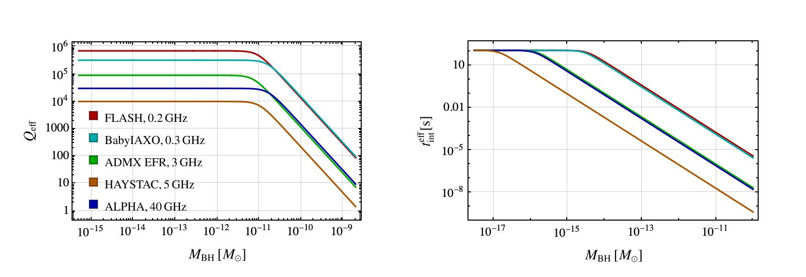
Figure 1: The effective quality factor $\displaystyle Q_{\rm eff}$ (left panel) and the minimum value between the source duration and the experimental observation time $\displaystyle t_{\rm obs}$, here $\displaystyle t_{\rm int}^{\rm eff}$ (right panel) for the experiments listed in Table 1. As a reference, the value $\displaystyle t_{\rm obs}=120$ s is chosen.

Therefore, two competing effects come into play when the detection of PBH mergers is considered. On one hand, at a fixed frequency one would like to consider heavier binaries, as the signal expected in Eq. (11) would be more prominent for at higher masses. On the other hand, it would be optimal to exploit the cavity resonance with the highest possible $\displaystyle Q_{\rm eff}$, thus requiring the search for light PBH binaries. As discussed below, it is indeed the former effect determining the optimal reach to be around $\displaystyle 10^{-11}\,M_{\odot}$ given the physical signal of PBH mergers.

Another factor impacting the experimental reach for an individual source is expressed by the effective integration time $\displaystyle t_{\rm int}^{\rm eff}$, which is here defined as the minimum value between the source duration and the experimental observation time $\displaystyle t_{\rm obs}$. Here, we set $\displaystyle t_{\rm obs}=120$ s as a reference. The effective integration time is typically of the order of a few minutes at a given frequency and is limited by the swiping time of the PBH merger within the frequency width of the cavity. This is shown in the right panel of Fig. 1. The effect is in place for basically all PBH mergers with a total mass heavier than $\displaystyle 10^{-14}\,M_{\odot}$. A direct inspection of Eq. (11) shows that the effect is not as impactful as the decrease in sensitivity coming from the scaling of $\displaystyle Q_{\rm eff}$ with the binary mass.

A significant enhancement of Eq. (11) would be brought in by the possible presence of a non-Gaussianity component in the density perturbations Franciolini et al. (2022). In the region of optimal reach around $\displaystyle 10^{-11}\,M_{\odot}$, the maximal enhancement is similar in amplitude, to the decrease in signal due to the typical bounds on lensing, requiring $\displaystyle f_{\rm PBH}\sim\mathcal{O}(10^{-2}-10^{-3})$ in the PBH population. This justifies the adoption of $\displaystyle f_{\rm PBH}=1$ as an optimistic case scenario.

IV Discussion

IV.1 Coherent sources

We first discuss the phenomenology related to the detection of a coherent source such as a binary merger. To showcase the effects affecting the cavity reach due to the non-stationary behaviour of the source, we first consider the setup of the resonant cavity employed in the FLASH experiment, as considered in Table 1. The reach for the experiment according to Eq. (4) is shown in Fig. 2 (red solid line) in comparison with the signal generated by mergers with $\displaystyle f_{\rm PBH}=1$ (black solid line). Note, that the expected signal scales linearly with $\displaystyle f_{\rm PBH}$. In Fig. 2, the frequency is fixed at the cavity value $\displaystyle f_{c}=200\,\rm MHz$, which is within reach for the FLASH setup. The drop in reach for $\displaystyle M\lesssim 10^{-11}\,M_{\odot}$ is due to the non-stationary behaviour of the source, resulting in a lower effective quality factor $\displaystyle Q_{\rm eff}$ as discussed below Eq. (12) and explicitly shown in Fig. 1.

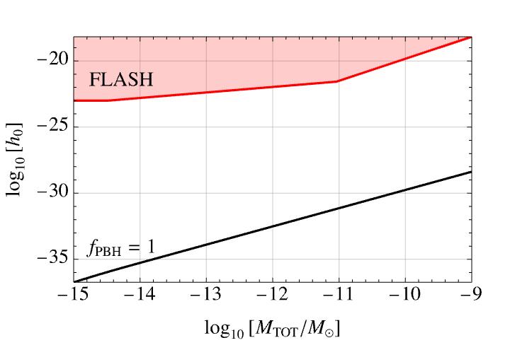
Figure 2: Comparison of the forecast reach for FLASH for different PBH masses. The red line correspond to the reach according to the values in Table 1. The black line corresponds to the theoretical prediction range for a monochromatic PBH distribution of values $\displaystyle f_{\rm PBH}=1$. The cavity frequency is fixed at $\displaystyle f_{c}=200$ MHz.

Another loss in sensitivity takes place for PBHs lighter than about $\displaystyle 10^{-15}\,M_{\odot}$. In this mass region, the limit factor originates from the effective time required by the source to swipe over a frequency width of the order of $\displaystyle f/Q=\Delta f$, as shown in the right panel of Fig. 1. In fact, the optimal reach region balancing between the physical signal and the cavity reach is around the $\displaystyle M_{\rm BH}\approx 10^{-11}\,M_{\odot}$ mass window, for which the optimal reach is achieved when

$$Q_{\rm eff}\simeq N_{\rm cycle}\simeq Q\,.$$ (14)

Similar results as in Fig. 2 qualitatively hold true for the other cavity setups expressed in Table 1.

We now consider the forecast reach in the cavity experiments given in Table 1. Results for the reach as a function of the cavity frequency are shown in Fig. 3 for the PBH mass $\displaystyle M_{\rm BH}=10^{-11}\,M_{\odot}$ (left) and $\displaystyle M_{\rm BH}=10^{-9}\,M_{\odot}$ (right). For each panel, the expected reach (dark shaded area) is compared with the ideal reach of a perfectly coherent source (lightly shaded area). For the binary masses considered, most of the actual reach loss accounts for the frequency swiping time being shorter than the typical integration time. In fact, according to Eq. (14) the effective quality factor $\displaystyle Q_{\rm eff}$ is maximized in this mass region. This corresponds to an ideal source that allows for the cavity to fully resonate without any loss due to a quality factor at source. This is the reach usually showed in the literature, see e.g. Refs. Berlin et al. (2022); Franciolini et al. (2022). For each panel, the black solid line marks the physical signal expected by a population of PBH binary mergers obtained using the results in Ref. Franciolini et al. (2022). Although cavity experiments swiping higher frequency ranges have a higher chance of working in the regime closer to the actual potential physical signal, there exists a discrepancy by many orders of magnitude from a potential detection of this source.

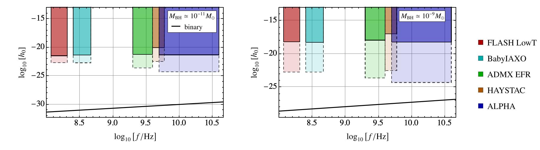
Figure 3: Cavity reach for the experiments listed in Table 1 as a function of frequency. For illustration purposes, we report the reach for the central value of the frequency range of each experiment. The lightly-shaded area denotes the expected reach for an ideal source, not limiting the capability of the cavity to fully resonate. The shaded area denotes the actual reach as compared to the actual source of a binary with mass $\displaystyle 10^{-11}\,M_{\odot}$ (left panel) and $\displaystyle 10^{-9}\,M_{\odot}$ (right panel), whose physical expected amplitude is marked by a black solid line. The PBH population is assumed to satisfy $\displaystyle f_{\rm PBH}=1$.

The right panel in Fig. 3 shows the dramatic improvement in considering a heavier mass range $\displaystyle M_{\rm BH}\approx 10^{-9}\,M_{\odot}$. While the physical signal increases in strain, the actual reach (dark shaded areas) significantly decreases. This is due to the quality of the source $\displaystyle N_{\rm eff}$ being placed away from the condition in Eq. (14) for the mass range considered. In this scenario, the physical cavity reach effectively places even further away from the physical signal when compared with the optimal case scenario $\displaystyle M_{\rm BH}\approx 10^{-11}\,M_{\odot}$ previously discussed and shown in the left panel.

IV.2 Stochastic source

We now turn to the discussion over the stochastic signal sourced by merging PBH binaries, characterized by a superposition of weak, incoherent, and unresolved GW sources Michelson (1987); Christensen (1992); Flanagan (1993). For this signal, the loss in coherence described in the previous section does not affect the reach for the mass region considered. However, the typical strain signal turns out to be significantly lower even for an optimistic scenario where the strain $\displaystyle h_{0}\lesssim 10^{-26}$ is expected Franciolini et al. (2022).

The analysis of a stochastic signal demands the coincident detection by two correlated and coaligned GW detectors, each picking up a GW strain $\displaystyle h_{i}(f)$ with $\displaystyle i=1,2$ labeling the detector. The signal-to-noise ratio can be expressed as Allen and Romano (1999)

$${\rm SNR}\approx\frac{3H_{0}^{2}}{10\pi^{2}}\,\sqrt{t_{\rm obs}}\,\left(\int_{-\infty}^{+\infty}{\rm d}f\,\frac{\gamma^{2}(f)\,\Omega_{\rm GW}^{2}(f)}{f^{6}\,P_{1}(f)\,P_{2}(f)}\right)^{1/2}\,.$$ (15)

Here, $\displaystyle P_{i}(f)$ is the noise power spectrum of the $\displaystyle i$-th detector, which is related to the variance of the cross-correlation signal as

$$\sigma_{i}^{2}=\int_{0}^{+\infty}{\rm d}f\,P_{i}(f)\,.$$ (16)

The quantity $\displaystyle\gamma(f)$, known as the overlap reduction function, quantifies the reduction in sensitivity due to the time delay between the two detectors and the non-parallel alignment of the cavity axes Flanagan (1993). For coincident and coaligned detectors it is $\displaystyle\gamma(f)=1$, while it is expected $\displaystyle\gamma(f)<1$ when the detectors are shifted apart or rotated.

To claim the successful detection of a GWB, we assume that such a signal is indeed present at the frequencies considered, with a mean value that allows for its correct identification for a fraction $\displaystyle\delta$ of the times. In this context, the SNR should satisfy Allen and Romano (1999)

$${\rm SNR}\geq[{\rm erfc}^{-1}(2\alpha)-{\rm erfc}^{-1}(2\delta)]/\sqrt{2}\,\,,$$ (17)

where $\displaystyle\alpha$ quantifies the false alarm rate. Setting a false alarm rate $\displaystyle\alpha=0.05$ and a detection rate $\displaystyle\delta=0.95$ leads to the requirement SNR $\displaystyle\gtrsim$ 1.64. Note, that the presence of $\displaystyle t_{\rm obs}$ appearing under the square root in Eq. (15) allows to consider much longer integration times when searching for the stochastic GWB compared with the coherent signal. Moreover, increasing $\displaystyle t_{\rm obs}$ in a search of a coherent, but transient, signal would not lead to an improved sensitivity because of the shortness of the signal duration.

We assess the sensitivity of the strain $\displaystyle h_{c}$ in Eq. (6) assuming a period of observation $\displaystyle t_{\rm obs}=6\,$months, leading to the results in Fig. 4 for the different experiments in Table 1. To estimate the expected physical signal we adopt the derivation of Refs. Ajith et al. (2011); Zhu et al. (2011), see also Ref. Franciolini et al. (2022) for a detailed discussion. We assume that the PBH masses are distributed according to a log-normal distribution centered at $\displaystyle M_{c}=10^{-11}\,M_{\odot}$ and of width $\displaystyle\sigma=0.26$ as Dolgov and Silk (1993); Carr et al. (2017)

$$\psi(M_{\rm BH})=\frac{f_{\rm PBH}}{\sqrt{2\pi}\sigma M_{\rm BH}}\exp\left[\frac{-\log\left(M_{\rm BH}/M_{c}\right)^{2}}{2\sigma^{2}}\right]\,.$$ (18)

Note, that an optimal reach is guaranteed for the range of masses considered since $\displaystyle Q_{\rm eff}\sim Q$. The distribution in Eq. (18) is normalized so that the fraction of PBHs that make up the DM is

$$f_{\rm PBH}=\int{\rm d}M_{\rm BH}\,\psi(M_{\rm BH})\,.$$ (19)

The result for the expected signal shown in Fig. 4 (black solid line) scales linearly with the PBH abundance $\displaystyle f_{\rm PBH}$, which is here set as $\displaystyle f_{\rm PBH}=1$. Even in this optimistic scenario, the values lie several orders of magnitude below the bound from BBN considerations in Eq. (7) (red-dashed line) and the actual cavity sensitivity of the various experiments.

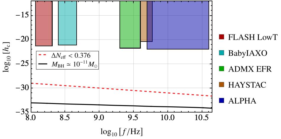
Figure 4: Stochastic GW background reach. The black line denotes the actual physical signal for $\displaystyle f_{\rm PBH}=1$ and the central value of the log-normal distribution $\displaystyle M_{c}=10^{-11}\,M_{\odot}$, see Eq. (18). The BBN bound is reported for comparison (dashed red line).

IV.3 Can we expect a continuous signal?

To address the stochastic GWB from PBH mergers, a monochromatic mass distribution with $\displaystyle f_{\rm PBH}=1$ is now assumed for simplicity, in analogy with the treatment for a coherent signal. Our findings thus allow for a direct comparison between the coherent and the stochastic cases. We generally obtain that for large PBH masses it is more convenient to search for a coherent signal, while the stochastic signal is stronger for light PBH mergers. Note, that for this type of analysis it is required to coordinate at least two detectors Aggarwal et al. (2021).

A necessary requirement for a stochastic noise to be detectable is that, at any time, at least $\displaystyle\mathcal{O}(1)$ mergers are sourcing within the cavity. As discussed above, the swiping time $\displaystyle t_{\rm swiping}$ across frequencies of the order of the frequency width of the cavity $\displaystyle\Delta f$ depends on the masses of the BH pair, with the typical $\displaystyle t_{\rm swiping}$ as given in Fig. 1. Therefore, at least one merger per swiping time should take place at every moment. This requirement provides the typical distance $\displaystyle d_{\rm swiping}$ at which a merger takes place, therefore allowing for an optimistic characterisation of the amplitude of the signal.

Given a rate per unit volume of PBH mergers $\displaystyle R_{\rm PBH}$, see e.g. Ref. Franciolini et al. (2022), the typical distances at which one merger event is constantly present in the cavity is found from integrating over a volume of radius $\displaystyle d_{\rm swiping}=(3V_{\rm swiping}/4\pi)^{1/3}$, to obtain

$$1\lesssim t_{\rm swiping}\int_{0}^{d_{\rm swiping}}{\rm d}r\,4\pi r^{2}R_{\rm PBH}.$$ (20)

While the above condition might not be sufficient to provide a stochastic signal, it surely suffices. More pragmatically, we address the question whether a continuous signal offers better detection prospects rather than fewer and rarer events of larger amplitude. As a byproduct, we determine the best search strategy for detecting PBH mergers in the mass window considered.

In previous literature the distance has been fixed through a different requirement, more precisely by looking for the volume within which one coherent merger per year is realized Franciolini et al. (2022). Under the condition in Eq. (20), the typical distance of a merger found by our requirement to realize at least one merger at each moment of time is significantly larger than the case of one coherent merger per year.

In Fig. 5, we show the comparison between the typical distances of black hole mergers sourcing a stochastic background (continuous line) with the coherent case of one merger per year $\displaystyle f_{\rm PBH}$ (dashed line) for different values of $\displaystyle f_{\rm PBH}$. In the latter case, the resulting curve is found to be consistent with the one in Ref. Franciolini et al. (2022). In the former case, the distance now also depends on the typical swiping time. For PBH masses above $\displaystyle\sim 10^{-14}M_{\odot}$, the typical distances increase significantly as they become larger than the galactic size, therefore resulting in fewer merging events for a given volume due to the absence the typical Galactic overdensity enhancement Pujolas et al. (2021). A similar effect is observed in the coherent case at heavier black hole masses Franciolini et al. (2022). The distances obtained for the stochastic case are significantly larger than in the coherent case and extend to extragalactic regions for heavier PBHs. For clarity, the plot in Fig. 5 focuses on the mass range for which the typical merger distances are larger than $\displaystyle 10^{5}\,$kpc. For even larger distances local galactic enhancements of nearby galaxies become relevant and, eventually, the redshift of the signal should also be included for $\displaystyle z\gtrsim 0.1$.

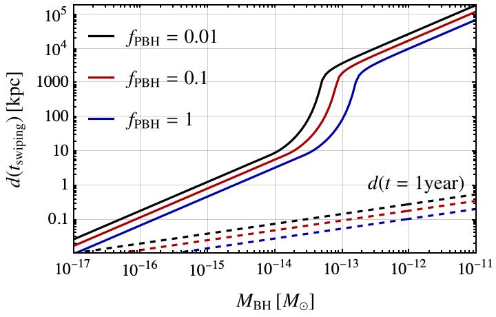
Figure 5: Distance for mergers sourcing a gravitational wave stochastic background under the condition in Eq. (20) (solid line). The coherent case of one merger here is shown with dashed lines.

One might expect that the requirement adopted here would lead to a significant loss in the potential reach of the experiment as compared to the true physical signal. However, this is partially balanced by the simple fact that the actual reach of the experiment is now integrated over the full experiment time and not just over the swiping time, see Eq. (4), therefore partially making up for such a loss. For simplicity, in the following we assume at total observation time of 1 year. Note, that the following approach allows for a direct utilisation of the axion search data since, due to the small frequency range explored by cavity experiment, changing slightly frequency every few minutes does not alter the magnitude of our estimates.

We now compare the potential reach for both the stochastic and the coherent cases. In this comparison we directly use Eq. (4), replacing the integration time with the running time of the cavity experiment which, for simplicity, we take to be 1 year. Since we expect $\displaystyle\mathcal{O}(1)$ mergers to resonate within the cavity at every time, for a fixed BH mass we must use the effective quality factor $\displaystyle Q_{\rm eff}$ in Eq. (4), analogously to the coherent case. Part of the resonance is suppressed by the presence of multiple sources, potentially resulting in a lower $\displaystyle Q_{\rm eff}$ which is compensated by the presence of multiple detectors.

Regarding the physical source, the difference between the stochastic and the coherent cases is given by the ratio of the distances obtained by adopting Eq. (20) and shown in Fig. 5. Therefore, it is useful to define the potential for a discovery as $\displaystyle S_{i}=h^{i}_{\rm physical}/h^{i}_{\rm reach}$, with $\displaystyle i=$coherent, stochastic. This quantity should be larger than one in order to ensure detection. For simplicity, in the following we focus on the FLASH experiment in Table 1 provided that other experiments lead to similar results.

The ratio between the stochastic and coherent potentials for a detection is given by

$$\frac{S_{\rm coherent}}{S_{\rm stochastic}}\simeq\frac{d(1{\rm\,year})}{d(t_{\rm swiping})}\left(\frac{1{\rm\,year}}{t_{\rm eff}^{\rm int}}\right)^{1/4}\,.$$ (21)

This ratio is shown in Fig. 6 as a function of the PBH merger masses and for a population with $\displaystyle f_{\rm PBH}=1$. Similarly to the distance plot comparison in Eq. (5), there is a dip in the figure coming from the missing galactic enhancement in the PBHs density. At smaller masses the stochastic signal is comparable to the coherent one, therefore suggesting the possibility of a joint search. Note, that the signal distances between the stochastic and coherent case become comparable due to the high density of light PBHs in the galaxy. In this rage of masses, the swiping times are macroscopically large and reach up to $\displaystyle\mathcal{O}(0.1\,{\rm year})$, therefore the condition in Eq. (20) is likely not leading to a clean stochastic background. Likely, a different condition is necessary, possibly leading to potentially larger distances and to smaller values of $\displaystyle Q_{\rm eff}$ due to interference. Consequently, the coherent signal would likely dominate even for light mergers. In any case, in the light mass range window, close to asteroid masses where all of the dark matter could come in the form of primordial black holes, the actual signal is extremely far from the current reach due to the lightness of the primordial masses, as expressed in Fig. 2.

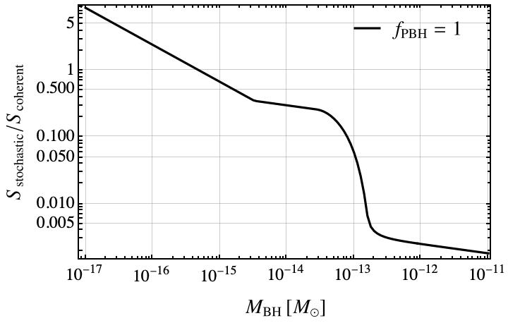
Figure 6: Ratio of potential reach for discovery between stochastic and direct merger detection. See Eq. (21)

.

For higher masses, the stochastic signal gets a suppression due to the large volumes necessary to attain a stochastic background. Therefore, for heavy PBHs it is more feasible to detect a coherent signal from one merger, suggesting the need to develop accurate templates for describing the signal from such events. Our estimate of the stochastic signal is clearly approximate and somewhat optimistic, so we therefore expect these results to remain valid in light of a potential and more accurate analysis.

V Conclusion: is there a detection outlook?

We have discussed the usage of resonant cavities, generally employed as haloscopes to search for the cosmic axion, for the search of gravitational wave signals of astrophysical origin at frequencies (0.1-10) GHz. This high-frequency gravitational wave (HFGW) domain spans a significantly broader spectrum compared to what is currently accessible by both ground-based and planned space-based interferometers. Various proposals for these investigations have been advanced in the scientific literature, including one outlined in the FLASH experiment Alesini et al. (2023).

If the HFGW signal originates from coalescing primordial black holes (PBHs), cavity experiments can probe the existence of PBH mergers in the mass window $\displaystyle M_{\rm BH}\lesssim 10^{-9}\,M_{\odot}$. Adopting the setup of the FLASH cavity and considering simultaneous observations of both axions and gravitational waves (GWs) from compact mergers yields the forecast reach as a function of the binary mass in Fig. 2. Other experiments employing similar setups lead to comparable results.

The signal expected from individual coherent sources in the Galaxy is too faint to be observed with current setups, based on conservative models for the distribution and merging details of the compact objects. This stems from quantifying the loss in the experimental reach due to the actual coherence of the source as discussed in Sec. III. The results do not improve when the collective stochastic signal that originates from the merging of multiple compact objects is considered. In this view, we have given a recipe for the estimate of the stochastic background that differs from previous literature and focuses on the presence of the signal in the cavity at all times, see Sec. IV.3. This allows us to predict the region of the PBH masses where the signal is dominated by coherent binary mergers, see Fig. 6. Our method relies on the evaluation of the distance that assures to attain at least one event in the cavity at all times, which is obtained from the condition in Eq. (20) and it is shown in Fig. 5 in comparison with the previous literature. Contrary to the coherent case, the distance thus obtained depends on the typical frequency swiping time. Given the vast range of masses in which the detection of a coherent signal would be facilitated over the stochastic background, our findings suggest to push for a broadband search for HFGWs with $\displaystyle\Delta f\sim f$.

Despite this result does not push towards the search of a HFGW signal through resonant cavities, we remind that i) such a search comes at practical no expenses, given that the cavity searches for the cosmic axion are already in place. For this, the detection apparatus should be equipped with an appropriate pick up and acquisition system of the signal generated in cavity modes not excited by the axion, as discussed elsewhere Alesini et al. (2023). Moreover, ii) the frequency band covered has not been explored by any dedicated search to date, so that unexpected sources could be present and add up to the GWB as a result of exotic new physics. In view of these considerations, the search for HFGWs is bright.

Appendix A Detailed resolution of the Einstein-Maxwell equations

Adapting the derivation in Ref. Millar et al. (2023) for the search of axions in a resonant cavity, we consider Maxwell’s equations in a dielectric medium sourced by a GW strain,

$$\begin{split}{\bf\nabla}\cdot{\bf D}&=\rho\,,\\ {\bf\nabla}\times{\bf H}-\partial_{t}{\bf D}&={\bf J}\,,\\ {\bf\nabla}\cdot{\bf B}&=0\,,\\ {\bf\nabla}\times{\bf E}+\partial_{t}{\bf B}&=0\,.\end{split}$$ (22)

Here, the displacement and the electric fields are related by $\displaystyle{\bf D}=\epsilon{\bf E}$, where $\displaystyle\epsilon$ is the permittivity tensor, while the magnetic flux density and field strength are assumed to coincide, $\displaystyle{\bf B}={\bf H}$. We solve the set of equations for an infinitely extended cylindrical cavity filled with a plasma, assuming that the axis is aligned along $\displaystyle{\bf\hat{z}}$ where the permittivity $\displaystyle\epsilon_{z}$ differs from unity.

Under axial symmetry the fields are decomposed as

$${\bf B}={\bf B}_{t}+B_{z}{\bf\hat{z}}\,;\quad{\bf E}={\bf E}_{t}+\epsilon_{z}E_{z}{\bf\hat{z}}\,,$$ (23)

where the subscripts “$\displaystyle t$” and “$\displaystyle z$” refer to the orientations transverse and parallel to the z-axis, respectively. Taking the Fourier transform of the fields and sources and assuming that the fields oscillate with frequency $\displaystyle\omega$ gives

$$\begin{split}&\left({\bf\nabla_{t}}\!+\!\frac{\partial}{\partial_{z}}{\bf\hat{z}}\right)\!\times\!\left({\bf B}_{t}+B_{z}{\bf\hat{z}}\right)\!=\!-i\omega\left({\bf E}_{t}+\epsilon_{z}E_{z}{\bf\hat{z}}\right)\!+\!\left({\bf J}_{t}\!+\!J_{z}{\bf\hat{z}}\right),\\ &\left({\bf\nabla_{t}}\!+\!\frac{\partial}{\partial_{z}}{\bf\hat{z}}\right)\!\times\!\left({\bf E}_{t}+E_{z}{\bf\hat{z}}\right)\!=\!-i\omega\left({\bf B}_{t}\!+\!\epsilon_{z}B_{z}{\bf\hat{z}}\right),\end{split}$$ (24)

where $\displaystyle{\bf\nabla_{t}}$ is the gradient in the direction transverse to the z-axis. Decomposing Eq. (24) into the directions transverse and parallel to $\displaystyle{\bf\hat{z}}$ yields

$$\begin{split}{\bf{\hat{z}}}\cdot{\bf\nabla_{t}}\times{\bf B_{t}}&=-i\omega\epsilon_{z}E_{z}+J_{z}\,,\\ {\bf{\hat{z}}}\cdot{\bf\nabla_{t}}\times{\bf E_{t}}&=i\omega B_{z}\,,\\ {\bf{\hat{z}}}\times\frac{\partial{\bf B_{t}}}{\partial_{z}}+{\bf\nabla_{t}}B_{z}\times{\bf\hat{z}}&=-i\omega{\bf E_{t}}+{\bf J_{t}}\,,\\ {\bf{\hat{z}}}\times\frac{\partial{\bf E_{t}}}{\partial_{z}}+{\bf\nabla_{t}}E_{z}\times{\bf\hat{z}}&=i\omega{\bf B_{t}}\,.\end{split}$$ (25)

The last two expressions in Eq. (25) lead to a relation for the transverse fields, once a Fourier transform along the z-axis with momentum $\displaystyle k_{z}$ is applied, to give

$$\begin{split}{\bf E_{t}}&=\frac{1}{\omega^{2}-k_{z}^{2}}\left({\bf\nabla_{t}}\frac{\partial E_{z}}{\partial z}+i\omega{\bf\nabla_{t}}B_{z}\times{\bf\hat{z}}-i\omega{\bf J_{t}}\right)\,,\\ {\bf B_{t}}&=\frac{1}{\omega^{2}-k_{z}^{2}}\left({\bf\nabla_{t}}\frac{\partial B_{z}}{\partial z}-i\omega{\bf\nabla_{t}}E_{z}\times{\bf\hat{z}}-\frac{\partial{\bf J_{t}}}{\partial_{z}}\right)\,.\end{split}$$ (26)

Contrary to the axion case discussed in Ref. Millar et al. (2023), in which the transverse components of the fields are sourced by $\displaystyle z$ components of the current only, in this more general case these components are sourced by the transverse current as well. In fact, in the case of axion $\displaystyle{\bf J}_{t}=0$ and the $\displaystyle B_{z}$ component can be neglected. Inserting Eq. (26) in the first two expressions of Eq. (25) gives

$$\begin{split}&\frac{\omega^{2}}{\omega^{2}-k_{z}^{2}}{\bf\nabla_{t}}^{2}E_{z}+\omega^{2}\epsilon_{z}E_{z}+i\omega J_{z}=\frac{i\omega}{\omega^{2}-k_{z}^{2}}{\bf\hat{z}}\cdot{\bf\nabla_{t}}\times\frac{\partial{\bf J}_{t}}{\partial z}\,,\\ &\frac{\omega^{2}}{\omega^{2}-k_{z}^{2}}{\bf\nabla_{t}}^{2}B_{z}-\omega^{2}B_{z}=\frac{\omega^{2}}{\omega^{2}-k_{z}^{2}}{\bf\hat{z}}\cdot{\bf\nabla_{t}}\times{\bf J}_{t}\,.\end{split}$$ (27)

Note, that the negative sign in front of the second term of $\displaystyle B_{z}$ equation can lead to tachyonic instability, which are avoided when the dissipation in the cavity walls are considered.

We now specialize these results to a resonant cavity by expanding the electric field in modes of pulsation $\displaystyle\omega_{n}$ labeled by an integer $\displaystyle n$, as

$$E_{z}=\sum_{n}e_{n}\,E_{n}({\bf x})\,,$$ (28)

where $\displaystyle e_{n}$ is the coefficient of the expansion and the eigenmodes satisfy Millar et al. (2023)

$$\begin{split}&{\bf\nabla_{t}}^{2}E_{n}=\epsilon_{z}^{\prime}\left(k_{z}^{2}-\omega_{n}^{2}\right)\,E_{n}\,,\\ &\int{\rm d}^{3}{\bf x}\,E_{n}E_{m}=\delta_{nm}\,.\end{split}$$ (29)

Here, the permeability has been decomposed as $\displaystyle\epsilon_{z}=\epsilon_{z}^{\prime}-i\epsilon_{z}^{\prime\prime}$ following standard notation Landau et al. (1961). Since the induced current has frequency $\displaystyle\omega_{n}$, $\displaystyle\epsilon^{\prime\prime}=\omega_{n}/(\omega\,Q)$, therefore leading, from Eq. (27), to

$$\omega^{2}\epsilon_{z}^{\prime}\frac{\omega^{2}-\omega_{n}^{2}}{\omega^{2}-k_{z}^{2}}\,e_{n}-i\frac{\omega\,\omega_{n}}{Q}\,e_{n}=-i\omega\int{\rm d}^{3}{\bf x}\,E_{n}\,\tilde{J}_{t}\,,$$ (30)

where we defined

$$\tilde{J}_{t}=J_{z}-\frac{1}{\omega^{2}-k_{z}^{2}}{\bf\hat{z}}\cdot{\bf\nabla_{t}}\times\frac{\partial\bf J_{t}}{\partial z}\,.$$ (31)

Solving for $\displaystyle e_{n}$ we finally obtain

$$e_{n}=\frac{-i\omega}{(\omega^{2}-\omega_{p}^{2})\frac{\omega^{2}-\omega_{n}^{2}}{\omega^{2}-k_{z}^{2}}-i\frac{\omega\,\omega_{n}}{Q}}\,\int{\rm d}^{3}{\bf x}\,{E}_{n}\tilde{J}_{t}\,.$$ (32)

Following Eq. (20) in Ref. Berlin et al. (2022), we decompose the current as

$$\tilde{J}_{t}=B_{0}\omega^{2}V^{1/3}\sum_{a}h_{a}(\omega)\hat{\bf j}_{a}\,,$$ (33)

so that

$$e_{n}=\frac{-iB_{0}\omega^{3}V^{1/3}}{(\omega^{2}-\omega_{p}^{2})\frac{\omega^{2}-\omega_{n}^{2}}{\omega^{2}-k_{z}^{2}}-i\frac{\omega\,\omega_{n}}{Q}}\,\sum_{A}h_{A}(\omega)\,\left(\int{\rm d}^{3}{\bf x}\,{E}_{n}\hat{\bf j}_{A}\right)\,.$$ (34)

This leads to the signal

$$e_{n}=-i\omega\,B_{0}\,V^{5/6}\,\mathcal{T}(\omega)\,\sum_{A}h_{A}(\omega)\,\eta_{A}\,,$$ (35)

where we introduced the cavity-GW coupling coefficient

$$\eta_{A}=\frac{1}{V^{1/2}}\int{\rm d}^{3}{\bf x}\,{E}_{n}\hat{\bf j}_{A}\,.$$ (36)

In Eq. (35), the function controlling the resonance is given by

$$\mathcal{T}(\omega)=\left[\left(1-\frac{\omega_{p}^{2}}{\omega^{2}}\right)\frac{\omega^{2}-\omega_{n}^{2}}{\omega^{2}-k_{z}^{2}}-\frac{i}{Q}\frac{\omega_{n}}{\omega}\right]^{-1}\,.$$ (37)

The energy stored in the $\displaystyle n$-th cavity mode is

$$U=\int{\rm d}f{\rm d}f^{\prime}\,\langle e_{n}(\omega)\,e_{n}(\omega^{\prime})\rangle\,,$$ (38)

or, using the expression above,

$$\displaystyle U \displaystyle= \displaystyle\int{\rm d}f{\rm d}f^{\prime}\,\omega(\omega^{\prime})\,B_{0}^{2}\,V^{5/3}\,\mathcal{T}(\omega)\mathcal{T}^{*}(\omega^{\prime})$$ (39)

$$\displaystyle\times\sum_{AA^{\prime}}\langle h_{A}(\omega)h_{A^{\prime}}(\omega^{\prime})\rangle\,\eta_{A}\,\eta_{A^{\prime}}\,.$$

For a stochastic signal, we write

$$\langle h_{A}(\omega)h_{A^{\prime}}(\omega^{\prime})\rangle=\frac{3H_{0}^{2}}{32\pi^{3}}\delta_{AA^{\prime}}\delta(f-f^{\prime})\,f^{-3}\,\Omega_{\rm GW}(\omega)\,,$$ (40)

so that when $\displaystyle k_{z}=0$ we find

$$U=\int\frac{{\rm d}\omega}{2\pi}\,\frac{(4\pi)\,(2\pi)^{3}\,\omega\,B_{0}^{2}\,V^{5/3}\,\eta^{2}\,\Omega_{\rm GW}(\omega)}{\omega^{2}\left[\left(1-\frac{\omega_{p}^{2}}{\omega^{2}}\right)\,\left(1-\frac{\omega_{n}^{2}}{\omega^{2}}\right)\right]^{2}+\left(\frac{\omega_{n}}{Q}\right)^{2}}\,\frac{3H_{0}^{2}}{32\pi^{3}}\,,$$ (41)

where an extra $\displaystyle(4\pi)$ comes from the angular integration and an extra $\displaystyle(2\pi)^{3}$ from converting $\displaystyle f$ into $\displaystyle\omega$. We have also introduced the coupling

$$\eta=\left(\sum_{A}\,\eta_{A}^{2}\right)^{1/2}\approx 0.14\,,$$ (42)

where the last expression corresponds to the cavity mode TM₀₁₂. Inserting the expression for $\displaystyle\Omega_{\rm GW}$ in Eq. (5) into Eq. (41) gives

$$U=\frac{1}{2}B_{0}^{2}V^{5/3}\eta^{2}\int_{0}^{+\infty}\!\!{\rm d}\omega\frac{\omega^{3}\,h_{c}^{2}}{\omega^{2}\left(1\!-\!\frac{\omega_{p}^{2}}{\omega^{2}}\right)^{2}\!\left(1\!-\!\frac{\omega_{n}^{2}}{\omega^{2}}\right)^{2}\!+\!\left(\frac{\omega_{n}}{Q}\right)^{2}}\,.$$ (43)

We first consider a coherent source with $\displaystyle N_{\rm cycle}$ cycles that can be observed inside the cavity, so that the strain is modeled as Hong et al. (2014); O’Hare and Green (2017)

$$h_{c}^{2}=\frac{h_{0}^{2}}{4\pi N_{\rm cycle}}\frac{\omega_{n}^{2}}{(\omega-\omega_{n})^{2}+\omega_{n}^{2}/(2N_{\rm cycle})^{2}}\,.$$ (44)

To estimate the signal power in the cavity $\displaystyle P_{\rm sig}=\omega U/Q$, we first evaluate the integral in Eq. (43) around $\displaystyle\omega\approx\omega_{n}$ in the case $\displaystyle\omega_{p}=0$. This leads to the expression for the power in the signal as

$$P_{\rm sig}\approx\frac{1}{4}B_{0}^{2}V^{5/3}\eta^{2}\omega_{n}^{3}\,h_{0}^{2}\,Q_{\rm eff}\,,\quad\hbox{for $\displaystyle\omega_{p}=0$}\,,$$ (45)

where $\displaystyle Q_{\rm eff}=\min(N_{\rm cycle},Q)$. This result coincides with the findings in previous literature, apart for an overall numerical factor $\displaystyle\mathcal{O}(1)$ Berlin et al. (2022).

On the other hand, the GWB is estimated by assuming a constant $\displaystyle h_{c}$ in the integrand of Eq. (43), in place of Eq. (44). Note, that in the case where $\displaystyle\omega_{n}\approx\omega_{p}$, which is the condition under which the ALPHA cavity experiment is going to operate, there is an additional enhancement by approximately a factor $\displaystyle Q$ that is relevant when detecting the GWB,

$$P_{\rm sig}\approx\sqrt{\frac{\pi}{6}}\,B_{0}^{2}\,V^{5/3}\,\eta^{2}\,\omega_{n}^{3}\,h_{c}^{2}\,Q\,,\quad\hbox{for $\displaystyle\omega_{p}\approx\omega_{n}$}\,.$$ (46)

We now estimate the strain sensitivity in the cavity. To estimate the signal-to-noise ratio (SNR), we account for the instrument noise which is characterized by the power

$$P_{\rm noise}=T_{\rm sys}\,\sqrt{\frac{\Delta f}{\Delta t}}\,,$$ (47)

where $\displaystyle T_{\rm sys}$ is the coldest effective temperature of the instrumentation and noise amplifier. The ratio between Eqs. (45) and (47) expresses the SNR as

$${\rm SNR}=P_{\rm sig}/P_{\rm noise}\,.$$ (48)

Setting $\displaystyle{\rm SNR}=1$ leads to the estimate for the reach of the GW strain in the resonant cavity as in Eq. (4) when focusing on the setup where $\displaystyle\omega_{p}=0$.

References

- Abbott et al. (2016) B. P. Abbott et al. (LIGO Scientific, Virgo), Phys. Rev. Lett. 116, 061102 (2016), arXiv:1602.03837 [gr-qc] .
- Abbott et al. (2019) B. P. Abbott et al. (LIGO Scientific, Virgo), Phys. Rev. X 9, 031040 (2019), arXiv:1811.12907 [astro-ph.HE] .
- McLaughlin (2013) M. A. McLaughlin, Class. Quant. Grav. 30, 224008 (2013), arXiv:1310.0758 [astro-ph.IM] .
- Goncharov et al. (2021) B. Goncharov et al., Astrophys. J. Lett. 917, L19 (2021), arXiv:2107.12112 [astro-ph.HE] .
- Lee (2016) K. J. Lee, in Frontiers in Radio Astronomy and FAST Early Sciences Symposium 2015, Astronomical Society of the Pacific Conference Series, Vol. 502, edited by L. Qain and D. Li (2016) p. 19.
- Chen et al. (2021) S. Chen et al., Mon. Not. Roy. Astron. Soc. 508, 4970 (2021), arXiv:2110.13184 [astro-ph.HE] .
- Ade et al. (2015) P. A. R. Ade et al. (BICEP2, Planck), Phys. Rev. Lett. 114, 101301 (2015), arXiv:1502.00612 [astro-ph.CO] .
- Ade et al. (2018) P. A. R. Ade et al. (BICEP2, Keck Array), Phys. Rev. Lett. 121, 221301 (2018), arXiv:1810.05216 [astro-ph.CO] .
- Namikawa et al. (2019) T. Namikawa, S. Saga, D. Yamauchi, and A. Taruya, Phys. Rev. D 100, 021303 (2019), arXiv:1904.02115 [astro-ph.CO] .
- Punturo et al. (2010) M. Punturo et al., Class. Quant. Grav. 27, 194002 (2010).
- Hild et al. (2011) S. Hild et al., Class. Quant. Grav. 28, 094013 (2011), arXiv:1012.0908 [gr-qc] .
- Amaro-Seoane et al. (2017) P. Amaro-Seoane et al., (2017), arXiv:1702.00786 [astro-ph.IM] .
- Yagi and Seto (2011) K. Yagi and N. Seto, Phys. Rev. D 83, 044011 (2011), [Erratum: Phys.Rev.D 95, 109901 (2017)], arXiv:1101.3940 [astro-ph.CO] .
- Badurina et al. (2020) L. Badurina et al., JCAP 05, 011 (2020), arXiv:1911.11755 [astro-ph.CO] .
- El-Neaj et al. (2020) Y. A. El-Neaj et al. (AEDGE), EPJ Quant. Technol. 7, 6 (2020), arXiv:1908.00802 [gr-qc] .
- Abe et al. (2021) M. Abe et al., Quantum Science and Technology 6, 044003 (2021), arXiv:2104.02835 [physics.atom-ph] .
- Abazajian et al. (2022) K. Abazajian et al. (CMB-S4), Astrophys. J. 926, 54 (2022), arXiv:2008.12619 [astro-ph.CO] .
- Dolgov and Ejlli (2011) A. D. Dolgov and D. Ejlli, Phys. Rev. D 84, 024028 (2011), arXiv:1105.2303 [astro-ph.CO] .
- Fujita et al. (2014) T. Fujita, M. Kawasaki, K. Harigaya, and R. Matsuda, Phys. Rev. D 89, 103501 (2014), arXiv:1401.1909 [astro-ph.CO] .
- Herman et al. (2021) N. Herman, A. Füzfa, L. Lehoucq, and S. Clesse, Phys. Rev. D 104, 023524 (2021), arXiv:2012.12189 [gr-qc] .
- Gehrman et al. (2023) T. C. Gehrman, B. Shams Es Haghi, K. Sinha, and T. Xu, JCAP 02, 062 (2023), arXiv:2211.08431 [hep-ph] .
- Franciolini et al. (2022) G. Franciolini, A. Maharana, and F. Muia, Phys. Rev. D 106, 103520 (2022), arXiv:2205.02153 [astro-ph.CO] .
- Banerjee and Dey (2023) I. K. Banerjee and U. K. Dey, JCAP 07, 024 (2023), arXiv:2305.07569 [gr-qc] .
- Liebling and Palenzuela (2023) S. L. Liebling and C. Palenzuela, Living Rev. Rel. 26, 1 (2023), arXiv:1202.5809 [gr-qc] .
- Visinelli (2021) L. Visinelli, Int. J. Mod. Phys. D 30, 2130006 (2021), arXiv:2109.05481 [gr-qc] .
- Arvanitaki and Dubovsky (2011) A. Arvanitaki and S. Dubovsky, Phys. Rev. D 83, 044026 (2011), arXiv:1004.3558 [hep-th] .
- Jung et al. (2020) S. Jung, T. Kim, J. Soda, and Y. Urakawa, Phys. Rev. D 102, 055013 (2020), arXiv:2003.02853 [hep-ph] .
- Lambiase et al. (2023) G. Lambiase, L. Mastrototaro, and L. Visinelli, JCAP 01, 011 (2023), arXiv:2207.08067 [hep-ph] .
- Ringwald et al. (2021) A. Ringwald, J. Schütte-Engel, and C. Tamarit, JCAP 03, 054 (2021), arXiv:2011.04731 [hep-ph] .
- Caprini et al. (2016) C. Caprini et al., JCAP 04, 001 (2016), arXiv:1512.06239 [astro-ph.CO] .
- Caprini and Figueroa (2018) C. Caprini and D. G. Figueroa, Class. Quant. Grav. 35, 163001 (2018), arXiv:1801.04268 [astro-ph.CO] .
- Addazi et al. (2024) A. Addazi, Y.-F. Cai, A. Marciano, and L. Visinelli, Phys. Rev. D 109, 015028 (2024), arXiv:2306.17205 [astro-ph.CO] .
- Bachmaier et al. (2023) M. Bachmaier, G. Dvali, J. S. Valbuena-Bermúdez, and M. Zantedeschi, (2023), arXiv:2309.14195 [hep-ph] .
- Kibble (1976) T. W. B. Kibble, J. Phys. A 9, 1387 (1976).
- Vilenkin (1981) A. Vilenkin, Phys. Lett. B 107, 47 (1981).
- Vilenkin (1985) A. Vilenkin, Phys. Rept. 121, 263 (1985).
- Witten (1985) E. Witten, Nucl. Phys. B 249, 557 (1985).
- Servant and Simakachorn (2023) G. Servant and P. Simakachorn, (2023), arXiv:2312.09281 [hep-ph] .
- Figueroa and Torrenti (2017) D. G. Figueroa and F. Torrenti, JCAP 10, 057 (2017), arXiv:1707.04533 [astro-ph.CO] .
- Adshead et al. (2018) P. Adshead, J. T. Giblin, and Z. J. Weiner, Phys. Rev. D 98, 043525 (2018), arXiv:1805.04550 [astro-ph.CO] .
- Kim et al. (2005) J. E. Kim, H. P. Nilles, and M. Peloso, JCAP 01, 005 (2005), arXiv:hep-ph/0409138 .
- Vagnozzi and Loeb (2022) S. Vagnozzi and A. Loeb, Astrophys. J. Lett. 939, L22 (2022), arXiv:2208.14088 [astro-ph.CO] .
- Cruise and Ingley (2006) A. M. Cruise and R. M. J. Ingley, Class. Quant. Grav. 23, 6185 (2006).
- Akutsu et al. (2008) T. Akutsu et al., Phys. Rev. Lett. 101, 101101 (2008), arXiv:0803.4094 [gr-qc] .
- Nishizawa et al. (2008) A. Nishizawa et al., Phys. Rev. D 77, 022002 (2008), arXiv:0710.1944 [gr-qc] .
- Ackley et al. (2020) K. Ackley et al., Publ. Astron. Soc. Austral. 37, e047 (2020), arXiv:2007.03128 [astro-ph.HE] .
- Pegoraro et al. (1978) F. Pegoraro, L. A. Radicati, P. Bernard, and E. Picasso, Phys. Lett. A 68, 165 (1978).
- Caves (1979) C. M. Caves, Phys. Lett. B 80, 323 (1979).
- Reece et al. (1984) C. E. Reece, P. J. Reiner, and A. C. Melissinos, Phys. Lett. A 104, 341 (1984).
- Ballantini et al. (2003) R. Ballantini, P. Bernard, E. Chiaveri, A. Chincarini, G. Gemme, R. Losito, R. Parodi, and E. Picasso, Class. Quant. Grav. 20, 3505 (2003).
- Mensky and Rudenko (2009) M. B. Mensky and V. N. Rudenko, Grav. Cosmol. 15, 167 (2009).
- Navarro et al. (2023) P. Navarro, B. Gimeno, J. Monzón-Cabrera, A. Díaz-Morcillo, and D. Blas, (2023), arXiv:2312.02270 [hep-ph] .
- Aguiar (2011) O. D. Aguiar, Res. Astron. Astrophys. 11, 1 (2011), arXiv:1009.1138 [astro-ph.IM] .
- Goryachev et al. (2014) M. Goryachev, E. N. Ivanov, F. van Kann, S. Galliou, and M. E. Tobar, Appl. Phys. Lett. 105, 153505 (2014), arXiv:1410.4293 [physics.ins-det] .
- Anandan and Chiao (1982) J. Anandan and R. Y. Chiao, Gen. Rel. Grav. 14, 515 (1982).
- Aggarwal et al. (2021) N. Aggarwal et al., Living Rev. Rel. 24, 4 (2021), arXiv:2011.12414 [gr-qc] .
- Schmieden and Schott (2024) K. Schmieden and M. Schott, PoS EPS-HEP2023, 102 (2024), arXiv:2308.11497 [gr-qc] .
- Gertsenshtein (1962) M. E. Gertsenshtein, Sov. Phys. JETP 14, 84 (1962).
- Zel’dovich (1973) Y. B. Zel’dovich, Zh. Eksp. Teor. Fiz. 68, 1311 (1973).
- Palessandro and Rothman (2023) A. Palessandro and T. Rothman, Phys. Dark Univ. 40, 101187 (2023), arXiv:2301.02072 [gr-qc] .
- Astone et al. (1993) P. Astone et al., Phys. Rev. D 47, 362 (1993).
- Astone et al. (1997) P. Astone et al., Astropart. Phys. 7, 231 (1997).
- Du et al. (2018) N. Du et al. (ADMX), Phys. Rev. Lett. 120, 151301 (2018), arXiv:1804.05750 [hep-ex] .
- Braine et al. (2020) T. Braine et al. (ADMX), Phys. Rev. Lett. 124, 101303 (2020), arXiv:1910.08638 [hep-ex] .
- Bartram et al. (2021) C. Bartram et al. (ADMX), Phys. Rev. Lett. 127, 261803 (2021), arXiv:2110.06096 [hep-ex] .
- Chakrabarty et al. (2024) S. Chakrabarty et al., Phys. Rev. D 109, 042004 (2024), arXiv:2303.07116 [hep-ph] .
- Brubaker (2017) B. M. Brubaker, First results from the HAYSTAC axion search, Ph.D. thesis, Yale U. (2017), arXiv:1801.00835 [astro-ph.CO] .
- Alesini et al. (2019) D. Alesini et al., (2019), arXiv:1911.02427 [physics.ins-det] .
- Alesini et al. (2023) D. Alesini et al., Phys. Dark Univ. 42, 101370 (2023), arXiv:2309.00351 [physics.ins-det] .
- Abeln et al. (2021) A. Abeln et al. (IAXO), JHEP 05, 137 (2021), arXiv:2010.12076 [physics.ins-det] .
- Ahyoune et al. (2023) S. Ahyoune et al., Annalen Phys. 535, 2300326 (2023), arXiv:2306.17243 [physics.ins-det] .
- Lawson et al. (2019) M. Lawson, A. J. Millar, M. Pancaldi, E. Vitagliano, and F. Wilczek, Phys. Rev. Lett. 123, 141802 (2019), arXiv:1904.11872 [hep-ph] .
- Millar et al. (2023) A. J. Millar et al. (ALPHA), Phys. Rev. D 107, 055013 (2023), arXiv:2210.00017 [hep-ph] .
- Backes et al. (2021) K. M. Backes et al. (HAYSTAC), Nature 590, 238 (2021), arXiv:2008.01853 [quant-ph] .
- Brady et al. (2022) A. J. Brady, C. Gao, R. Harnik, Z. Liu, Z. Zhang, and Q. Zhuang, PRX Quantum 3, 030333 (2022), arXiv:2203.05375 [quant-ph] .
- Domcke et al. (2022) V. Domcke, C. Garcia-Cely, and N. L. Rodd, Phys. Rev. Lett. 129, 041101 (2022), arXiv:2202.00695 [hep-ph] .
- Allen and Romano (1999) B. Allen and J. D. Romano, Phys. Rev. D 59, 102001 (1999), arXiv:gr-qc/9710117 .
- Thrane and Romano (2013) E. Thrane and J. D. Romano, Phys. Rev. D 88, 124032 (2013), arXiv:1310.5300 [astro-ph.IM] .
- Romano and Cornish (2017) J. D. Romano and N. J. Cornish, Living Rev. Rel. 20, 2 (2017), arXiv:1608.06889 [gr-qc] .
- Domcke et al. (2024) V. Domcke, C. Garcia-Cely, S. M. Lee, and N. L. Rodd, JHEP 03, 128 (2024), arXiv:2306.03125 [hep-ph] .
- Chung-Jukko et al. (2024) L. Chung-Jukko, E. A. Lim, and D. J. E. Marsh, (2024), arXiv:2403.03774 [astro-ph.CO] .
- Carr et al. (2021) B. Carr, K. Kohri, Y. Sendouda, and J. Yokoyama, Rept. Prog. Phys. 84, 116902 (2021), arXiv:2002.12778 [astro-ph.CO] .
- Gouttenoire and Volansky (2023) Y. Gouttenoire and T. Volansky, (2023), arXiv:2305.04942 [hep-ph] .
- Flores et al. (2024) M. M. Flores, A. Kusenko, and M. Sasaki, (2024), arXiv:2402.13341 [hep-ph] .
- Dvali et al. (2021) G. Dvali, F. Kühnel, and M. Zantedeschi, Phys. Rev. D 104, 123507 (2021), arXiv:2108.09471 [hep-ph] .
- Oblath (2023) N. S. Oblath (ADMX), “Current status and future plans of the axion dark matter experiment,” (2023), tAUP 2023.
- Niikura et al. (2019) H. Niikura et al., Nature Astron. 3, 524 (2019), arXiv:1701.02151 [astro-ph.CO] .
- Giudice et al. (2016) G. F. Giudice, M. McCullough, and A. Urbano, JCAP 10, 001 (2016), arXiv:1605.01209 [hep-ph] .
- Pujolas et al. (2021) O. Pujolas, V. Vaskonen, and H. Veermäe, Phys. Rev. D 104, 083521 (2021), arXiv:2107.03379 [astro-ph.CO] .
- Moore et al. (2015) C. J. Moore, R. H. Cole, and C. P. L. Berry, Class. Quant. Grav. 32, 015014 (2015), arXiv:1408.0740 [gr-qc] .
- Coogan et al. (2021) A. Coogan, L. Morrison, and S. Profumo, Phys. Rev. Lett. 126, 171101 (2021), arXiv:2010.04797 [astro-ph.CO] .
- Berlin et al. (2022) A. Berlin, D. Blas, R. Tito D’Agnolo, S. A. R. Ellis, R. Harnik, Y. Kahn, and J. Schütte-Engel, Phys. Rev. D 105, 116011 (2022), arXiv:2112.11465 [hep-ph] .
- Michelson (1987) P. F. Michelson, Mon. Not. Roy. Astron. Soc. 227, 933 (1987).
- Christensen (1992) N. Christensen, Phys. Rev. D 46, 5250 (1992).
- Flanagan (1993) E. E. Flanagan, Phys. Rev. D 48, 2389 (1993), arXiv:astro-ph/9305029 .
- Ajith et al. (2011) P. Ajith et al., Phys. Rev. Lett. 106, 241101 (2011), arXiv:0909.2867 [gr-qc] .
- Zhu et al. (2011) X.-J. Zhu, E. Howell, T. Regimbau, D. Blair, and Z.-H. Zhu, Astrophys. J. 739, 86 (2011), arXiv:1104.3565 [gr-qc] .
- Dolgov and Silk (1993) A. Dolgov and J. Silk, Phys. Rev. D 47, 4244 (1993).
- Carr et al. (2017) B. Carr, M. Raidal, T. Tenkanen, V. Vaskonen, and H. Veermäe, Phys. Rev. D 96, 023514 (2017), arXiv:1705.05567 [astro-ph.CO] .
- Landau et al. (1961) L. D. Landau, E. M. Lifshitz, J. B. Sykes, J. S. Bell, and E. H. Dill (1961).
- Hong et al. (2014) J. Hong, J. E. Kim, S. Nam, and Y. Semertzidis, (2014), arXiv:1403.1576 [hep-ph] .
- O’Hare and Green (2017) C. A. J. O’Hare and A. M. Green, Phys. Rev. D 95, 063017 (2017), arXiv:1701.03118 [astro-ph.CO] .