Test the Loop Quantum Gravity Theory via the Lensing Effect

Abstract

Recently, scholars such as Lewandowski, Ma, and Yang have successfully derived a quantum-corrected black hole model in loop quantum gravity (Phys.Rev.Lett.130.101501 (2023)), which is a modification of the Schwarzschild black hole. In this paper, we calculate the strong/weak gravitational lensing effects under the quantum-corrected black hole model, taking the supermassive black holes M87* and SgrA* as the subjects of study to explore the impact of the quantum correction parameter $\alpha$ on the positions of images and the Einstein ring. Our calculations show that in the case of strong gravitational lensing, the lensing coefficient $\bar{a}$ increases with an increase in the quantum correction parameter, while the deflection angle and the lensing coefficient $\bar{b}$ decrease with an increase in the quantum correction parameter. The quantum correction parameter $\alpha$ has a significant impact in the context of supermassive black holes. In weak gravitational lensing, the quantum correction parameter $\alpha$ plays a suppressive role. Our theoretical analysis suggests that with advancements in future astrophysical observation techniques, it might be possible to test loop quantum gravity theory using the gravitational lensing effect.

Keywords

Loop quantum gravity, quantum-corrected black hole, gravitational lensing, Einstein ring.

I Introduction

General relativity(GR) theoretically predicted the existence of black holes, and it was not until the gravitational waves from the merger of binary black holes were first detected by LIGO during 2015 to 2016 that the existence of black holes was confirmed in the universe. This provided solid observational evidence for GR LIGOScientific:2016emj . Moreover, GR has been extensively confirmed in other respects. For example, a series of tests in cosmology or in pulsars (Will:2014kxa, ; Ferreira:2019xrr, ; Clifton:2011jh, ), as well as observations from the Event Horizon Telescope EventHorizonTelescope:2019dse ; EventHorizonTelescope:2022wkp have all verified the validity of GR. However, general relativity also has its limitations, particularly under specific conditions of matter and energy, where gravitational collapse inevitably leads to the emergence of spacetime singularities. This is the famous singularity theorem jointly proposed by Hawking and Penrose Hawking:1970zqf ; Penrose:1964wq . The common understanding regarding singularities is that near them, all physical laws diverge. To circumvent these ”singularities,” Penrose proposed the cosmic censorship conjecture. In response to this conjecture, many scholars have conducted relevant tests (for example, some references Ames:2023akp ; Zhao:2024qzg ; Meng:2024els ; Zhao:2024lts ; Tang:2023sig ; Meng:2023vkg ; Sadeghi:2023lkz ; Zhao:2023vxq ). However, some scholars believe that singularities can be avoided when considering quantum effects Ashtekar:2006wn , and the leading candidate for this quantum theory is loop quantum gravity(LQG).

LQG is a highly regarded quantum gravity theory, characterized by its background independence and non-perturbative nature Yang:2022btw ; Han:2005km ; Ashtekar:2004eh ; Perez:2012wv , thereby attracting significant attention and extensive research Perez:2012wv ; Giesel:2011idc ; Thiemann:2002nj ; Ashtekar:2004eh . In addressing the singularity of the Big Bang in GR, loop quantum cosmology has successfully circumvented these singularities Ashtekar:2006rx ; Ashtekar:2006wn ; Ashtekar:2006uz ; Ashtekar:2003hd ; Papanikolaou:2023crz ; Date:2004fj ; Vereshchagin:2004uc ; Singh:2003au ; Wilson-Ewing:2016yan . Therefore, research into LQG holds promise for resolving some of the puzzles in general relativity. Within the framework of quantum cosmology, many black hole solutions have been developed Bodendorfer:2019nvy ; Ashtekar:2018lag ; Brahma:2020eos ; Bodendorfer:2019jay . Recently, in the study of spherical symmetric matter collapse, scholars such as Lewandowski, Ma, and Yang have successfully derived a quantum-corrected black hole(BH) model within the framework of LQG theory Lewandowski:2022zce . This model serves as a modification of the Schwarzschild BH and also addresses the issue of singularity in matter collapse. This is because, when the density of the collapsing matter reaches the Planck scale, the collapse does not continue; instead, it halts and enters a bounce expansion phase Lewandowski:2022zce . Research on the properties of quantum-corrected BH hole spacetimes has been conducted by various scholars, including studies on the shadows and photon rings of quantum-corrected BH, as well as their Quasinormal modes Gong:2023ghh ; Ye:2023qks ; Yang:2022btw . Additionally, the properties of quantum-corrected BH from other perspectives have been investigated in Shao:2023qlt ; Zhang:2023yps ; Giesel:2022rxi . These articles have examined different features of quantum-corrected BH, making further exploration into the lensing effects of quantum-corrected BH a fascinating subject.

Gravitational lensing(GL), as an astronomical observational tool, occurs when the massive objects (such as black holes) warp the surrounding spacetime, causing the light paths to bend. This theory was initially proposed by researchers such as Refsdal and Liebes 10.1093/mnras/128.4.295 ; Liebes:1964zz , and its validity was first confirmed through the phenomenon of gravitational deflection of sunlight Bozza:2002zj . Subsequently, the application of this theory has expanded to black hole research, offering a new approach to integrating theoretical analysis with astronomical observational data. Gravitational lensing is divided into two types: strong GL, under the strong-field limit, and weak GL, under the weak-field limit.

For strong GL, Virbhadra and colleagues were the first to derive the lensing equation for a Schwarzschild BH in the strong field limit through numerical analysis Virbhadra:1999nm . Later, in 2001, Bozza and others derived the lens theory formula for Schwarzschild BHs in the strong field limit, and the following year extended it to general static spherically symmetric spacetimes Bozza:2001xd ; Bozza:2002zj . Subsequently, this method was improved and extended to general asymptotically flat spacetimes and axially symmetric spacetimes Tsukamoto:2016jzh ; Duan:2023gvm ; Kumar:2023jgh ; Ghosh:2022mka ; Hsieh:2021rru ; Islam:2021dyk ; Hsieh:2021scb ; Chen:2011ef . Based on the method proposed by Bozza, it has been applied to Reissner-Nordstrom BHs and braneworld BHs Eiroa:2003jf ; Whisker:2004gq ; Eiroa:2005vd ; Li:2015vqa , and corresponding studies have been conducted on black holes in other spacetime backgrounds Islam:2020xmy ; Bozza:2003cp ; Kumar:2019pjp ; Kumar:2021cyl ; QiQi:2023nex ; Panpanich:2019mll ; Babar:2021nst ; Kuang:2022xjp .

For weak GL in the weak field limit, many studies have successfully explained a series of astronomical observation phenomena Weinberg:2013agg . It has significant implications for exploring the cosmic microwave background radiation, dark matter, and dark energy Lewis:2006fu ; Bucko:2022kss ; Bucko:2022kss ; Massey:2010hh . Early research on weak gravitational lensing by Mauro Sereno analyzed the behavior of weak GL in Reissner-Nordstrom BHs using perturbative methods Sereno:2003nd . Keeton and colleagues derived formulas for weak GL in spherically symmetric black holes using Taylor expansion methods Keeton:2005jd . These methods were later extended to rotating spacetimes Werner:2007vu ; Sereno:2006ss . With the continuous in-depth study of weak GL, many scholars have derived another method for obtaining the weak lensing formula. Gibbons and Werner proposed a more efficient method for calculating the deflection angle based on the Gauss-Bonnet theorem and using the concept of optical metrics Gibbons:2008rj ; Werner:2012rc , mainly through integrating the Gaussian curvature to obtain the deflection angle. Based on this novel method, literature Ishihara:2016vdc ; Ishihara:2016sfv ; Ono:2017pie ; Islam:2020xmy addresses the correction of the deflection angle for light sources and observers at finite distances, while research for the case of infinite distance between the light source and observer can be found in respective studies Jusufi:2017lsl ; Jusufi:2017hed ; Jusufi:2017mav ; Fu:2021akc ; Ovgun:2018xys ; Javed:2022fsn ; Gao .

In fact, both strong and weak lensing are among the tools for studying black holes and cosmology. Gravitational lensing has found wide application in cosmology, astronomy, and physics Li:2015vqa . In particular, the breakthroughs of the Event Horizon Telescope (EHT) have opened the door to directly observing strong gravitational fields EventHorizonTelescope:2019uob ; EventHorizonTelescope:2022wkp , especially providing an unprecedented perspective when studying celestial bodies such as black holes. This achievement has made the study of strong gravitational lensing effects a hot topic in the field, as it allows us to directly observe objects in strong gravitational environments, thereby revealing the characteristics of black holes under different gravitational theories and enabling comparisons with predictions made in GR QiQi:2023nex . Meanwhile, research into the weak gravitational lensing effect provides us with an important tool for exploring the large-scale structure of the universe, especially in studies of cosmological parameters and dark matter distribution Li:2015vqa . Through the study of these two types of lensing effects, we can not only gain a deeper understanding of black holes and their surrounding strong gravitational fields but also expand our knowledge of the entire structure of the universe, thereby making new progress in the interdisciplinary field of astrophysics and cosmology. Recently, in the theory of LQG, researchers such as Lewandowski, Ma, and Yang innovatively proposed a QCBH model Lewandowski:2022zce . This development provides a new theoretical framework for the study of GL effects, especially in exploring the impact of quantum correction parameters on lensing effects.

The structure of this article is as follows: In Section II, we primarily review the QCBH. In Section III, we calculate the deflection angle and the corresponding lensing coefficients ($\bar{a}$ and $\bar{b}$) in the QCBH using the method proposed by Bozza et al. for handling the deflection angle of GL in the strong field limit, and analyze the impact of the quantum correction parameter $\alpha$ on the deflection angle and lensing coefficients. In Section IV, we mainly introduce the analysis of lensing observables and Einstein rings against the backdrop of supermassive black holes (M87* and SgrA*). In Section V, we analyze the impact of the quantum correction parameter $\alpha$ on the weak deflection angle. In the final section, we present our conclusions.

II Quantum-corrected black hole

Recently, scholars such as Lewandowski, Ma, and Yang have achieved success in the field of loop quantum cosmology using the Oppenheimer-Snyder model. They successfully derived a quantum-corrected BH model Lewandowski:2022zce , with the metric as follows

$$ds^{2}=-f\left(r\right)dt^{2}+\frac{1}{f\left(r\right)}dr^{2}+r^{2}\left(d\theta^{2}+{sin}^{2}\theta d\phi^{2}\right),$$ (1)

where

$$f\left(r\right)=1-\frac{2M}{r}+\frac{\alpha{G^{2}M}^{2}}{r^{4}},$$ (2)

Where $\alpha=16\sqrt{3}\gamma^{3}\ell_{p}^{2}$ is the quantum correction parameter,and $\ell_{p}^{2}=\sqrt{G\hbar}$, $M$ represents the mass of the black hole. It’s worth mentioning that when the quantum correction parameter vanishes ($\alpha=0$), the quantum-corrected BH degenerates into a Schwarzschild BH. Moreover, our discussion is primarily focused on spacetimes with event horizons, hence, the mass parameter cannot be arbitrarily chosen. In our paper, we constrain the mass to be greater than the minimum value of the mass parameter. Regarding the lower limit of this mass parameter, it is calculated under the natural units system in the literature Ye:2023qks as follows

$$M_{min}=\frac{16\gamma\sqrt{\gamma\pi}}{3\sqrt[4]{3}}\approx 0.8314.$$ (3)

This means that the black hole mass $M$ we discuss is greater than $M_{min}$($M>M_{min}$).

In the subsequent calculations, we will use natural units, where $G=c=\hbar=1$. Thus, equation (2) will become

$$f\left(r\right)=1-\frac{2M}{r}+\frac{\alpha M^{2}}{r^{4}}.$$ (4)

The quantum correction parameter will become $\alpha=16\sqrt{3}\gamma^{3}$. Analyzing the metric (4), it is easy to find $\lim\limits_{x\to\infty}f\left(r\right)=1$, indicating that this spacetime is asymptotically flat. To facilitate the discussion on GL, we perform a dimensionless parameter transformation on the line element (1) and rewrite it as

$$d{\widetilde{s}}^{2}=-G(x)dT^{2}+\frac{1}{G(x)}dx^{2}+F(x)\left(d\theta^{2}+{sin}^{2}\theta d\phi^{2}\right),$$ (5)

and

$$F(x)=x^{2}.$$ (6)

Metric (4) is rewritten as

$$G(x)=1-\frac{1}{x}+\frac{\widetilde{\alpha}}{{16x}^{4}}.$$ (7)

The dimensionless parameters here are

$$r=2Mx,$$ (8)

$$t=2MT,$$ (9)

$$\alpha=\widetilde{\alpha}M^{2}.$$ (10)

The analytical expression for the event horizon of a black hole can be obtained from $g^{rr}=0$, that is

$$G(x)=1-\frac{1}{x}+\frac{\widetilde{\alpha}}{{16x}^{4}}=0.$$ (11)

Clearly, when the quantum correction parameter assumes different values, the resulting roots can be none, one, or two, corresponding to the physical scenarios of a BH not having an event horizon, having one event horizon, and having two event horizons, respectively. Our main focus is on the scenarios where an event horizon exists. Thus, we will limit the quantum correction parameter to $\frac{27}{16}\geq\widetilde{\alpha}\geq 0$, aligning with our discussion on the existence of BHs (the presence of an event horizon).

As shown in Figure 1, when the quantum correction parameter gradually increases, the number of event horizons also changes significantly. This indicates that the quantum correction parameter has a profound impact on the properties of quantum-corrected BH. When the quantum correction parameter gradually increases beyond a critical value, at this point, there are no real root solutions for $G(x)$, which physically signifies that there are no black holes in this spacetime.By analyzing Figure 1, it can be intuitively observed that when there is no quantum correction parameter $(\widetilde{\alpha}=0)$, the metric (7) represents a standard Schwarzschild BH. It is clear that the event horizon radius of the quantum-corrected BH is smaller than the event horizon radius of the Schwarzschild BH (represented by the black dashed line in the figure 1).

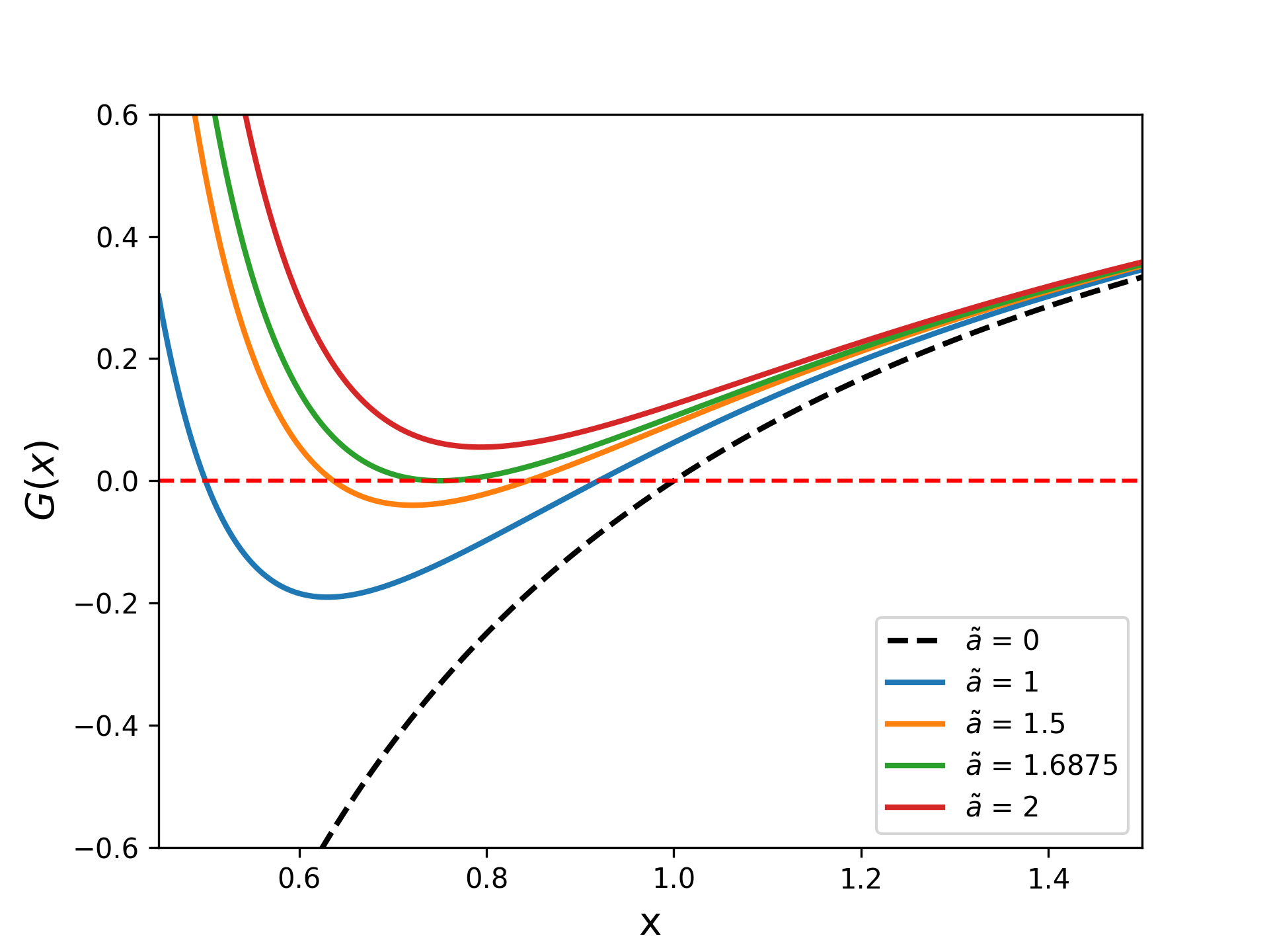
Figure 1: Different quantum correction parameters affect the existence of event horizons in quantum-corrected BH, where the black dashed line represents the event horizon situation of the Schwarzschild BH.

III Strong gravitational lensing effect

In this section, we adopt the strong field limit method by V. Bozza et al. to calculate the deflection angle near the unstable photon sphere Bozza:2002zj , which is an extension of the literature Bozza:2001xd and represents a general method for extending the strong field limit to any static, spherically symmetric spacetime. In the second section, we analyzed and determined that quantum-corrected BH are asymptotically flat, hence this method is applicable in the spacetime of quantum-corrected BH. Considering that quantum-corrected BHs are static and spherically symmetric, for ease of analysis, we restrict photons to the equatorial plane, i.e.,$\theta=\frac{\pi}{2}$. This metric (5) then becomes

$$d{\widetilde{s}}^{2}=-G(x)dT^{2}+\frac{1}{G(x)}dx^{2}+F(x)d\phi^{2}.$$ (12)

In stable and spherically symmetric spacetime structures, the four-momentum of photons along directions that preserve time and spatial symmetries (Killing vector fields) is conserved. Therefore, the energy $E$ and angular momentum $L$ of a photon are related to the Killing vector fields $\xi_{t}^{\mu}$ and $\xi_{\phi}^{\mu}$, which are associated with time translation symmetry and axial rotational symmetry, respectively. That is, the energy of the photon is defined as $E=-p_{\mu}\xi_{t}^{\mu}$, and the angular momentum of the photon is defined as $L={p_{\mu}\xi}_{\phi}^{\mu}$, where $p_{\mu}$ are the components of the photon’s four-momentum.Therefore, we obtain

$$\frac{d\phi}{d\tau}=\frac{L}{F(x)},$$ (13)

$$\frac{dt}{d\tau}=-\frac{E}{G(x)}.$$ (14)

Here, $\tau$ is the affine parameter along the geodesic, and our main interest is in the deflection of light in the limit near the photon sphere surface on null geodesics, that is, $d{\widetilde{s}}^{2}=0$. At this point, combining the metric (12) and formulas (13) and (14), we can obtain

$$-G(x)\frac{E^{2}}{G(x)}+\frac{1}{G(x)}{(\frac{dx}{d\tau})}^{2}+F(x)\frac{L^{2}}{{F(x)}^{2}}=0.$$ (15)

Rearranging the above equation yields

$${(\frac{dx}{d\tau})}^{2}=E^{2}-\frac{L^{2}}{F(x)}.$$ (16)

The path of photons moving around a BH can be described using an effective potential Pugliese:2010ps ; Gan:2021pwu ; Guo:2022muy ; Mustafa:2022xod , and the radial effective potential can be given by the following expression

$$V_{eff}(x)=\frac{L^{2}G(x)}{F(x)}=\frac{L^{2}}{x^{2}}(1-\frac{1}{x}+\frac{\widetilde{\alpha}}{{16x}^{4}}).$$ (17)

According to the radial effective potential, for light rays coming from infinity and incident on a BH, when the light rays reach the vicinity of the BH, due to the presence of the effective potential, the light rays may bend at a specific radius $x_{0}$(this distance is the closest distance of the photon to the BH). At this point, the light does not fall into the black hole but escapes from the BH to be observed by an observer at infinity. We are interested in the radius $x_{m}$ of the subtle motion of photons on their orbit, because on these unstable orbits, any small perturbation can cause the photon to deviate from its path, and these deviations either cause the photon to fall into the BH or escape from it Chandrasekhar:1984siy . Therefore, we can deduce from the expression of the effective potential energy that photons are only in a precarious state at the potential energy extremum, which can be described in mathematical language as

$$\frac{dV_{eff}(x)}{dx}=0\quad\text{photon sphere},$$ (18)

$$\frac{dV_{eff}(x)}{dx}=0\quad\text{and}\quad\frac{d^{2}V_{eff}(x)}{dx^{2}}<0\quad\text{unstable photon sphere},$$ (19)

$$\frac{dV_{eff}(x)}{dx}=0\quad\text{and}\quad\frac{d^{2}V_{eff}(x)}{dx^{2}}>0\quad\text{stable photon sphere}.$$ (20)

Clearly, without loss of generality, we are more interested in the unstable photon sphere and in studying the deflection angle of light rays in the strong field limit. Therefore, we reevaluate the effective potential, considering only the conditions of the unstable photon sphere, from which we can

$$\frac{{G(x)}^{{}^{\prime}}}{G(x)}=\frac{{F(x)}^{{}^{\prime}}}{F(x)}.$$ (21)

Substituting equation (12) into the above expression yields

$$16x^{4}-24x^{3}+3\widetilde{\alpha}=0.$$ (22)

Equation (22) describes the orbital radius where photon motion exists. Due to the presence of quantum correction parameters, this leads to the roots of Equation (22) not being unique. When the quantum deformation parameter disappears ($\widetilde{\alpha}=0$), there exist two roots. As the quantum deformation parameter gradually increases, the number of roots gradually decreases until no roots exist. Analyzing Equation (22), the solution of interest to us is the largest root because, at the largest root, the motion of the photon is unstable (satisfying condition (19)), which can be intuitively seen from the effective potential (as shown in Figure 2). According to the trend of the effective potential, the unstable photon sphere is located at a greater radial distance. Therefore, for Equation (22), we take the largest root as the photon’s orbital radius $x=x_{m}$ . In the following discussion, our $x_{m}$ will only represent the unstable orbital radius of the photon sphere.

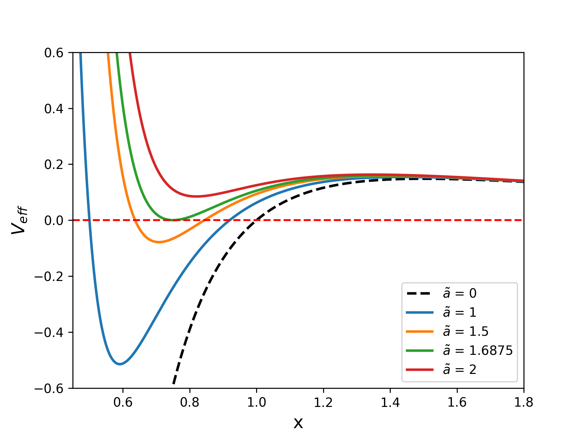
Figure 2: The trend graph of the effective potential clearly shows two photon spheres. The one with the smaller radial distance represents the stable photon sphere, and the one with the larger radial distance represents the unstable photon sphere. This distance is the orbital radius we are interested in.

When photons coming from an infinite distance approach a black hole, they carry a certain impact parameter $b$. At this point, the light will approach the BH at a certain minimum distance and then be symmetrically deflected back to infinity. The relationship between the impact parameter $b$ and the minimum distance $x_{0}$ of the light reaching the BH can be derived from $V_{eff}(x)=E^{2}$, and by combining Equation (17), the impact parameter can be expressed as

$$b=\frac{L}{E}=\sqrt{\frac{F(x_{0})}{G(x_{0})}}.$$ (23)

Here, we are interested in the unstable photon sphere, hence we choose $x_{0}=x_{m}$ , with the corresponding impact parameter being $b_{m}$. For the deflection angle $\alpha_{D}$ of light in the strong field limit, it is given by the definition in the literature Virbhadra:1999nm as

$$\alpha_{D}(x_{0})=I(x_{0})-\pi,$$ (24)

where

$$I(x_{0})=2\int_{x_{0}}^{\infty}\frac{d\phi}{dx}dx,$$ (25)

here

$$\frac{d\phi}{dx}=\frac{1}{\sqrt{G(x)F(x)}\sqrt{\frac{G(x_{0})F(x)}{F(x_{0})G(x)}-1}}.$$ (26)

A detailed derivation of the above expression can be found in the literature Virbhadra:1998dy ; Fu:2021fxn .

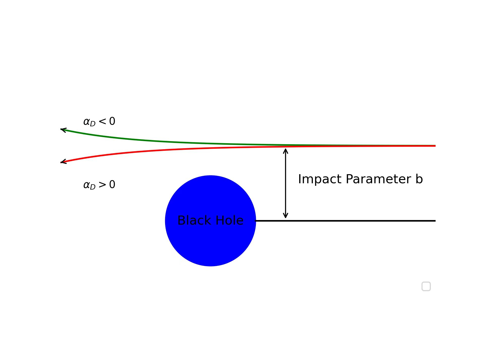
Figure 3: The deflection of light near a black hole.

For the deflection angle $\alpha_{D}(x_{0})$ in the strong field limit, as shown in Figure 3, under certain conditions, the deflection angle can be less than zero $(\alpha_{D}(x_{0})<0)$, meaning the light bends away from the BH. When $\alpha_{D}(x_{0})>0$, the light bends towards the BH. We are particularly interested in the deflection of light near the photon sphere. In the strong field limit, considering the approximation method used in the literature Bozza:2002zj , we find that the deflection angle near the photon sphere is divergent. Therefore, we redefine a variable Jha:2023qqz ; Fu:2021fxn ; Islam:2021dyk .

$$z=\frac{x_{0}}{x},$$ (27)

when the above approximation is employed, the integral (25) can be rewritten as

$$I(x_{0})=\int_{0}^{1}{R(z,x_{0})f((z,x_{0})}dz.$$ (28)

Here, $R(z,x_{0})$ can be expressed as

$$R\left(z,x_{0}\right)=\frac{2x_{0}\sqrt{F\left(x_{0}\right)}}{F\left(x\right)\left(1-z\right)^{2}},$$ (29)

$f(z,x_{0})$ can be expressed as

$$f(z,x_{0})=\frac{1}{\sqrt{G(x_{0})-\frac{G(x)F(x_{0})}{F(x)}}}.$$ (30)

It is easy to find that the integral of all values in the function $R(z,x_{0})$ is regular, but the deflection angle of the function $f(z,x_{0})$ diverges at $z=0$. Therefore, to avoid the divergence of the deflection angle at $z=0$, we perform a series expansion of the function $f(z,x_{0})$ at $z=0$, retaining the first and second order approximations to obtain

$$f(z,x_{0})\approx f_{0}(z,x_{0})=\frac{1}{\sqrt{\gamma_{1}(x_{0})z+\gamma_{2}(x_{0})z^{2}}},$$ (31)

the parameters here can be written as

$$\gamma_{1}\left(x_{0}\right)=\frac{x_{0}}{F\left(x_{0}\right)}\left[F^{{}^{\prime}}\left(x_{0}\right)G\left(x_{0}\right)-G^{{}^{\prime}}\left(x_{0}\right)F\left(x_{0}\right)\right],$$ (32)

$$\gamma_{2}(x_{0})= \frac{1}{2}\left[\frac{\left(2x_{0}F(x_{0})-2x_{0}^{2}F^{\prime}(x_{0})\right)}{F(x_{)})^{2}}\right.$$

$$\left.\times\left(F^{\prime}(x_{0})G(x_{0})-G^{\prime}(x_{0})F(x_{0})\right)\right.$$

$$\left.+\frac{x_{0}}{F\left(x_{0}\right)}(F^{{}^{\prime\prime}}\left(x_{0}\right)G\left(x_{0}\right)-G^{{}^{\prime\prime}}\left(x_{0}\right)F\left(x_{0}\right))\right].$$ (33)

According to the method used in the reference Bozza:2002zj , the integral can be divided into two parts: one part is divergent, and the other part is regular. Therefore, it can be written as

$$I(x_{0})=I_{D}(x_{0})+I_{R}(x_{0}),$$ (34)

the divergent part $I_{D}(x_{0})$ is expressed as

$$I_{D}(x_{0})=\int_{0}^{1}{R(0,x_{m})f_{0}((z,x_{0})}dz,$$ (35)

the regular part $I_{R}(x_{0})$ is expressed as

$$I_{R}(x_{0})=\int_{0}^{1}\left(R(z,x_{0})f((z,x_{0})-R(0,x_{m})f_{0}((z,x_{0})\right)dz.$$ (36)

$I_{D}(x_{0})$ represents the regular part after subtracting the divergent part of the integral. Therefore, solve the above two integrals (35) and (36). Near $x_{m}$ the deflection angle of light in the strong field limit can be expressed as Bozza:2002zj ; Bozza:2003cp

$$\alpha_{D}(b)=-\bar{a}log(\frac{b}{b_{m}}-1)+\bar{b}+O(b-b_{m}).$$ (37)

The corresponding coefficients can be written as

$$\bar{a}=\frac{R(0,x_{m})}{2\sqrt{\gamma_{2}\left(x_{m}\right)}},$$ (38)

$$\bar{b}=-\pi+I_{R}(x_{m})+\bar{a}log(\frac{2\gamma_{2}\left(x_{m}\right)}{G(x_{m})}).$$ (39)

We characterize the relationship between the strong GL coefficients and the quantum correction parameter through numerical solution methods. As shown in Figure 4, it is clear that the deflection coefficient $\bar{a}$ gradually increases with the increase of the quantum correction parameter, while the deflection coefficient $\bar{b}$ gradually decreases as the quantum correction parameter $\widetilde{\alpha}$ decreases.It is worth mentioning that when the quantum correction parameter vanishes $(\bar{\alpha}=0)$, the quantum-corrected BH becomes equivalent to a Schwarzschild BH, and our calculation results maintain the values for a Schwarzschild black hole Bozza:2002zj , that is, $\bar{a}=1$, $\bar{b}=-0.40023$ (see Table 1). In Figure 5, under different quantum correction parameters, the deflection angle diverges at certain values $(b=b_{m})$, where these impact parameters are smaller than those for a Schwarzschild BH, and the deflection angle sharply decreases as the quantum correction parameter increases (see the left graph in Figure 5). Of course, under the same impact parameters, the deflection angle of a Schwarzschild black hole is significantly larger than that of a quantum corrected black hole, and gradually decreases as the quantum correction parameter increases (see the right graph in Figure 5).

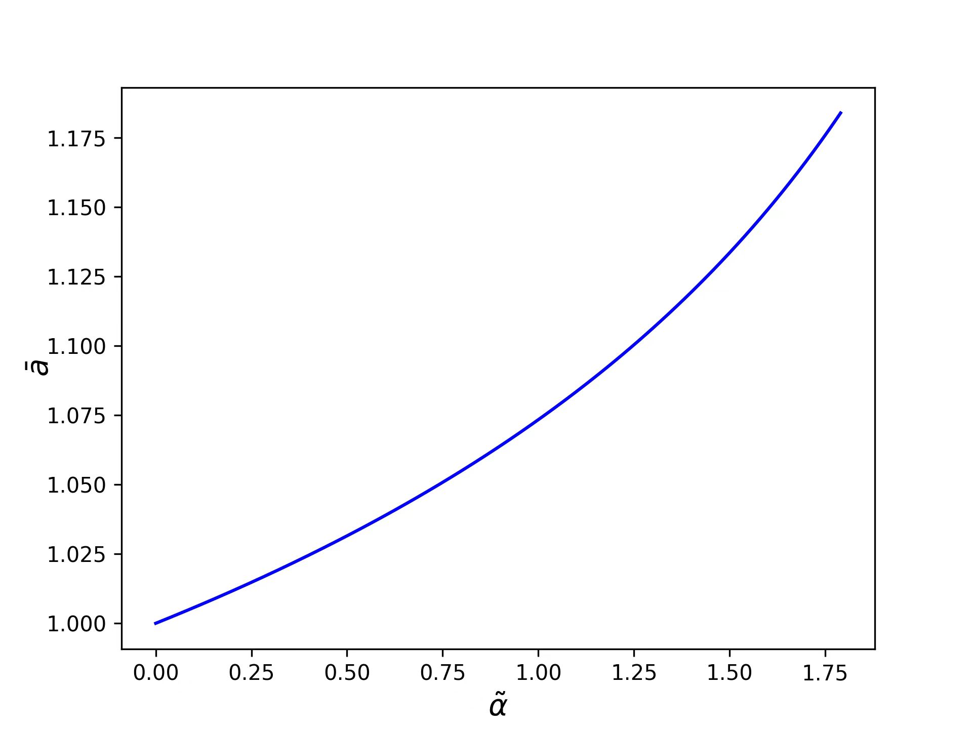
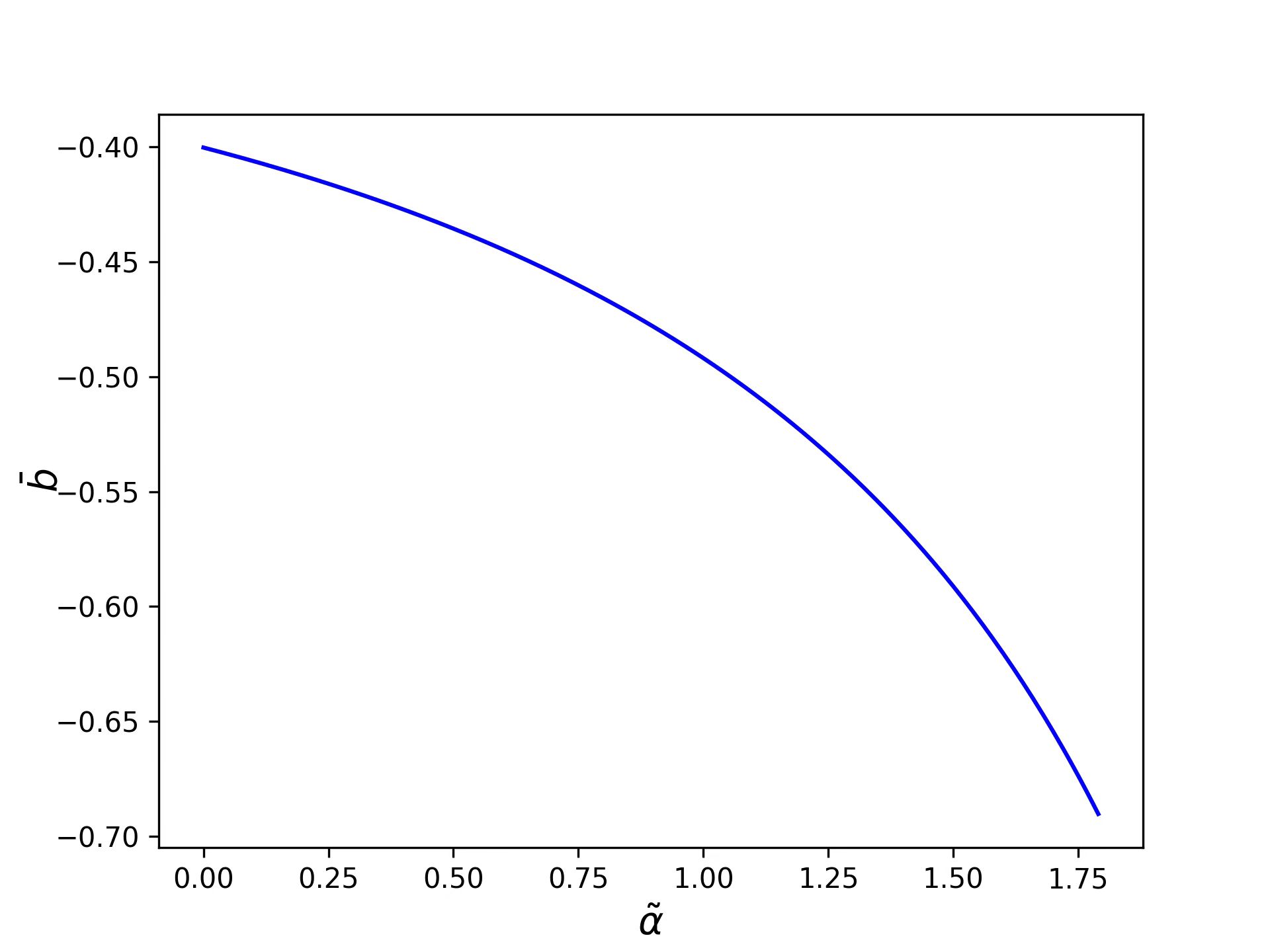
Figure 4: The left graph shows the variation of the strong field deflection coefficient $\bar{a}$ with the quantum correction parameter $\widetilde{\alpha}$, and the right graph shows the variation of the deflection angle coefficient $\bar{b}$ with the quantum correction parameter $\widetilde{\alpha}$.

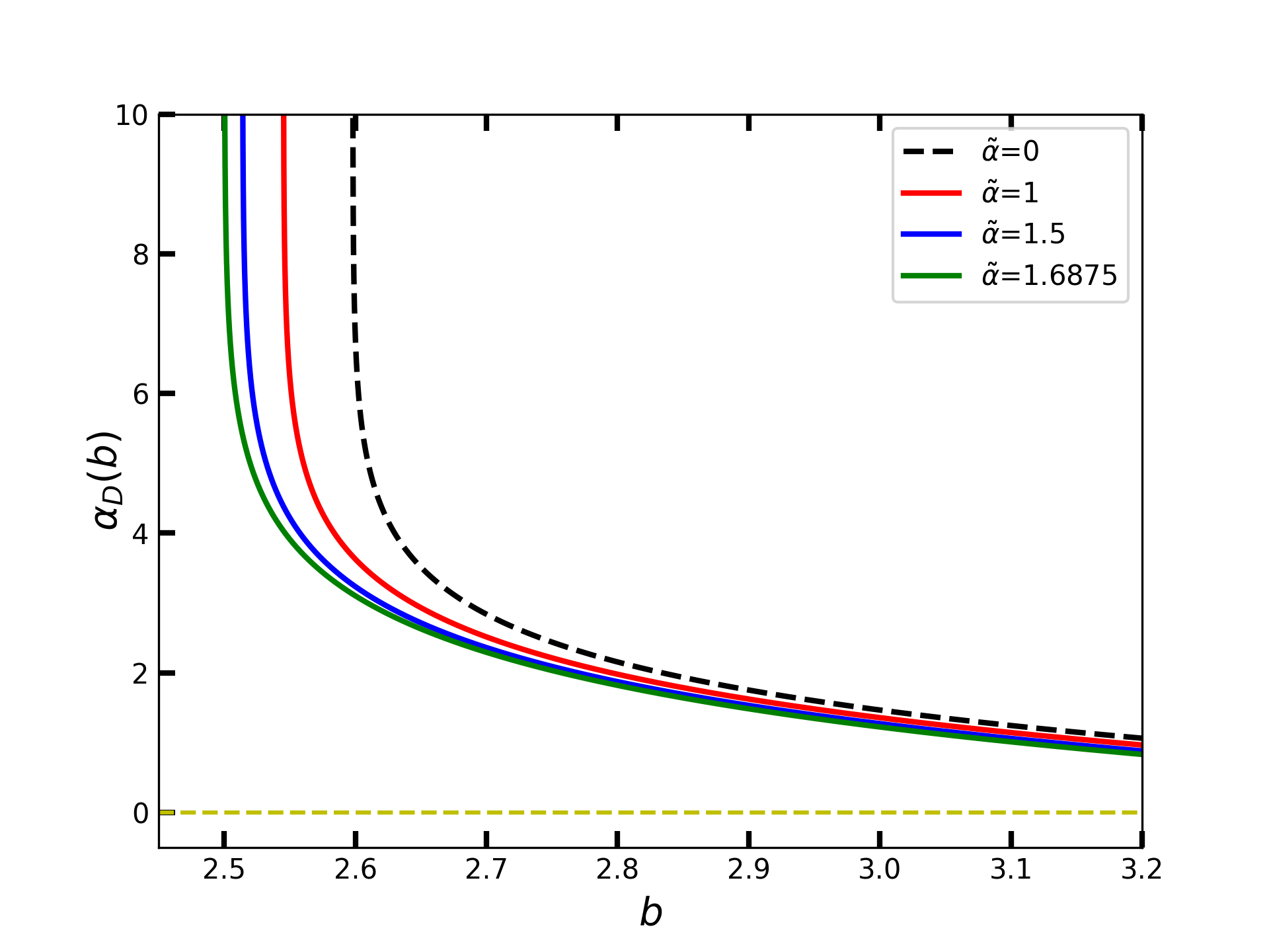
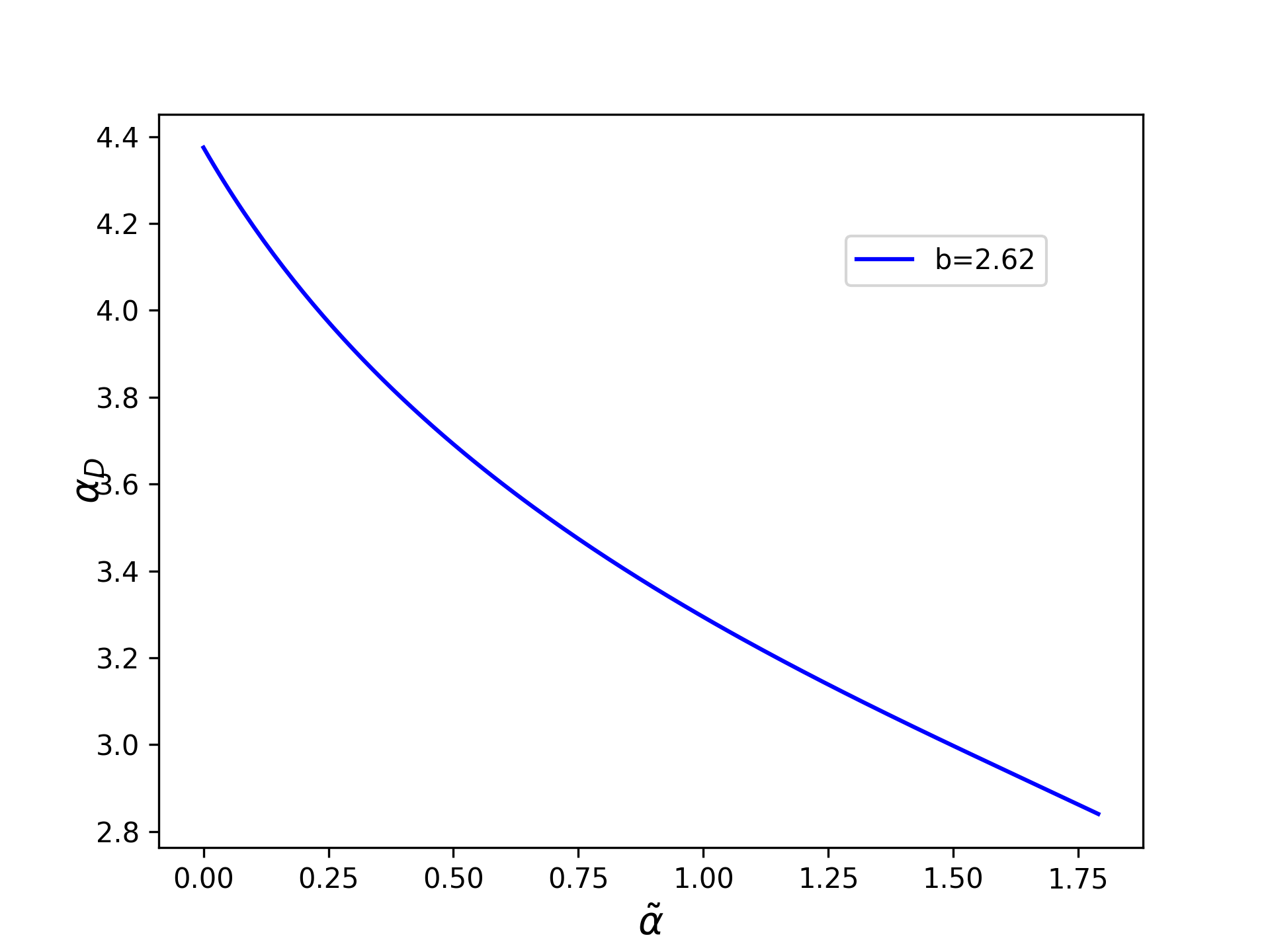
Figure 5: The left graph shows the variation of the deflection angle with the impact parameter under different quantum parameters, with the black dashed line representing the deflection angle of a Schwarzschild BH. The right graph shows how the deflection angle changes with the quantum correction parameter at an impact parameter $b=2.62$.

IV Observational phenomena under the gravitational lensing effect of supermassive black holes

IV.1 Characteristic observables in strong lensing effect

In the section II, we calculate the deflection angle of strong gravitational lensing, thus allowing us to easily compute the position of the images based on the lens equation. Following the definitions of the lens equation in the literature Virbhadra:1999nm ; Bozza:2008ev ; Bozza:2001xd , we can deduce that the lens equation is

$$\beta=\theta-\frac{D_{LS}}{D_{OS}}\Delta\alpha_{n}.$$ (40)

Here, $D_{LS}$ is the distance between the lens and the light source, and $D_{OS}$ is the distance between the observer and the light source $(D_{OS}=D_{OL}+D_{LS})$, $\beta$ and $\theta$ represent the angular positions of the source and image relative to the optical axis, and $\Delta\alpha_{n}=\alpha(\theta)-2n\pi$ denotes the deflection of light after orbiting the black hole $n$ times. To approximate the deflection $\Delta\alpha_{n}$, we need to find the angle $\theta_{n}^{0}$, which is obtained by solving $\alpha(\theta)=2n\pi$. Our adopted solution is given by the following equations

$$\theta_{n}^{0}=\frac{b_{m}(1+e_{n})}{D_{OL}},$$ (41)

and

$$e_{n}=exp(\frac{\bar{b}-2n\pi}{\bar{a}}).$$ (42)

Next, by combining the deflection angle formula (37) in the strong field limit and the gravitational lens equation (40), while neglecting higher-order terms, we can approximate the position of the nth image Bozza:2002zj

$$\theta_{n}=\theta_{n}^{0}+\frac{b_{m}e_{n}(\beta-\theta_{n}^{0})D_{OS}}{\bar{a}D_{LS}D_{OL}}.$$ (43)

From the above equation, it is clear that when $\beta-\theta_{n}^{0}=0$, the position of the image coincides with that of the source. At this moment, the position of the image $\theta_{n}=\theta_{n}^{0}$, indicating that the position of the $n$th image has not been corrected (this represents that the source and the image are on the same side). To obtain the position of the image on the opposite side of the source, we need to extend this by replacing $\beta$ with $-\beta$, thus obtaining the position of the $n$th image on the opposite side of the source. It’s worth mentioning that when the light ray, lens (here a BH), and observer are in a straight line, i.e.,$\beta=0$, solving equation (43) will yield

$$\theta_{n}^{E}=(1-\frac{b_{m}e_{n}D_{OS}}{\bar{a}D_{LS}D_{OL}})\ \theta_{n}^{0}.$$ (44)

This is what is referred to as the Einstein ring Einstein:1936llh .

In addition to the position of the source image, its magnification is also a significant piece of information. Therefore, the magnification of the $n$th image can be defined as Virbhadra:1998dy ; Bozza:2002zj ; Virbhadra:2007kw

$$\mu_{n}=\left.\left(\frac{\beta}{\theta}\frac{d\beta}{d\theta}\right)^{-1}\right|_{\theta_{n}^{0}}=\frac{{b_{m}}^{2}(1+e_{n})D_{OS}}{\bar{a}\beta D_{LS}{D_{OL}}^{2}}e_{n},$$ (45)

it is easy to deduce from the above equation that the magnification decreases exponentially with increasing image number $n$. When $\beta$ approaches zero, the magnification reaches its maximum, meaning that the image is at its brightest. To achieve some interesting observational effects, it is common to simplify the analysis to two layers of images, i.e., the outermost image as a single $\theta_{1}$, and all inner images combined as a whole $\theta_{\infty}$. This approach leads to several interesting observable values Bozza:2002zj . The position of all inner images considered as a whole, denoted as $\theta_{\infty}$, is

$$\theta_{\infty}=\frac{b_{m}}{D_{OL}},$$ (46)

the separation $s$ between the first image and the other images is

$$s=\theta_{1}-\theta_{\infty}=\theta_{\infty}exp(\frac{\bar{b}-2\pi}{\bar{a}}),$$ (47)

the flux ratio of the brightness between the first image and the other images is

$$r=\frac{\mu_{1}}{\sum_{n=2}^{\infty}\mu_{n}}=exp(\frac{2\pi}{\bar{a}}),$$ (48)

$$r_{mag}\approx 2.5log(r)=\frac{5\pi}{\bar{a}ln(10)}.$$ (49)

From equation (49), it can be seen that, in this case, the flux ratio is independent of the distance between the lens and the observer.

When using these observables, as defined by the above equation, we find that as long as we can determine the coefficients $\bar{a}$ and $\bar{b}$ in the deflection angle, as well as the critical impact parameter $b_{m}$, we can theoretically calculate the observable values for a quantum-corrected BH under strong GL. Of course, if these observational data could be obtained through astronomical observations, it would provide a way to analyze the properties of quantum-corrected BHs and the characteristics of strong GL in such BHs.

IV.2 Lensing effects of the supermassive black holes M87* and SgrA*

To evaluate the interesting observable values calculated in the previous section, here we consider the quantum-corrected BH as the supermassive black holes M87* and SgrA*, to study these observables. Moreover, we compare the simulated data with that of a Schwarzschild BH (when the quantum correction parameters vanish, the quantum-corrected BH reduces to a Schwarzschild BH). Based on the latest astronomical observation data, we understand that the mass of M87* is $\left(6.5\pm 0.7\right)\times{10}^{9}M_{\odot}$, and its distance from Earth is $\left(16.8\pm 0.8\right)Mpc$ EventHorizonTelescope:2019ggy .The mass of SgrA* is $3.98\times{10}^{6}M_{\odot}$, and its distance from Earth is $7.97kpc$ Chen:2019tdb . With these observational data, we can further determine how the quantum correction parameter $\tilde{\alpha}$ affects the quantum-corrected BH, which is our area of interest.

Next, we will calculate the Einstein rings for M87* and SgrA*. For clarity, here we only depict the image for $n=1$, that is, $\theta_{1}^{E}$. The Einstein ring calculations were done in the previous section, and

$$\theta_{n}^{E}=(1-\frac{b_{m}e_{n}D_{OS}}{\bar{a}D_{LS}D_{OL}})\ \theta_{n}^{0}.$$ (50)

When the black hole is located between the observer and the light source, then $D_{OS}=D_{LS}=2D_{OL}$. Assuming that $D_{OL}$ is much larger than the impact parameter $b_{m}(D_{OL}\gg b_{m})$, and combining this with equation (41), we can obtain

$$\theta_{n}^{E}\approx\frac{(1+e_{n})b_{m}}{D_{OL}}-\frac{2(e_{n}(1+e_{n})){b_{m}}^{2}}{\bar{a}{D_{OL}}^{2}}.$$ (51)

When $n=1$, equation (51) becomes

$$\theta_{1}^{E}\approx\frac{(1+e_{1})b_{m}}{D_{OL}}-\frac{2e_{1}(1+e_{1}){b_{m}}^{2}}{\bar{a}{D_{OL}}^{2}}.$$ (52)

Here $e_{1}=exp(\frac{\bar{b}-2\pi}{\bar{a}})$, Hence, the Einstein ring images in M87* and SgrA* are shown in Figure 6. For both M87* and SgrA*, the existence of quantum correction parameters leads to Einstein rings with angular radii smaller than those formed by Schwarzschild BHs (the dashed lines indicate the Einstein rings of Schwarzschild BHs). This demonstrates the dependency of the Einstein rings on the quantum correction parameters.

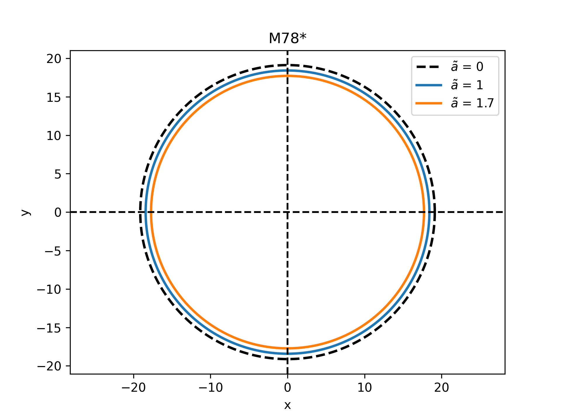
Figure 6: Images of the Einstein ring for $n=1$; the left image is M87*, and the right image is SgrA*.

In M87* and SgrA*, simulate several observables of interest, that is, observables (46), (47), and (48). Here, $b_{m}$ is represented as

$$b_{m} =\sqrt{\frac{F(x_{m})}{G(x_{m})}}=\sqrt{\frac{{x_{m}}^{2}}{1-\frac{1}{x_{m}}+\frac{\widetilde{\alpha}}{{16x_{m}}^{4}}}}$$

$$=4\sqrt{\frac{{x_{m}}^{6}}{\widetilde{\alpha}+16(-1+x_{m}){x_{m}}^{3}}}.$$ (53)

Clearly, as shown in Figure 7 and Table 1, the presence of the quantum correction parameter causes the image position $\theta_{\infty}$ to decrease with the increase of the quantum correction parameter, the image separation $S$ to increase with the increase of the quantum correction parameter, and the relativistic image brightness ratio $r_{mag}$ to decrease with the increase of the quantum correction parameter. It is noteworthy that in both M87* and SgrA*, the range of the angular position of the relativistic images due to the variation in the quantum correction parameter is $20.1042\mu as\geq\theta_{\infty}(M87*)\geq 19.3466\mu as$ and $25.9482\mu as\geq\theta_{\infty}(SgrA*)\geq 24.9704\mu as$. The deviation in the angular position of the relativistic images between the quantum-corrected black hole and the Schwarzschild black hole is no more than $1\mu as$ (see Table 1 and Figure 7). In other words, with the current resolution of the EHT, it is difficult to distinguish between a Schwarzschild BH and a quantum-corrected BH. Of course, if the observational precision improves in the future, we will observe its data through astronomical methods, and combine it with equations (47) and (49) to obtain the corresponding lensing deflection coefficients. By then, integrating theory with actual observations, we will be able to further understand quantum-corrected BHs, which will be very interesting.

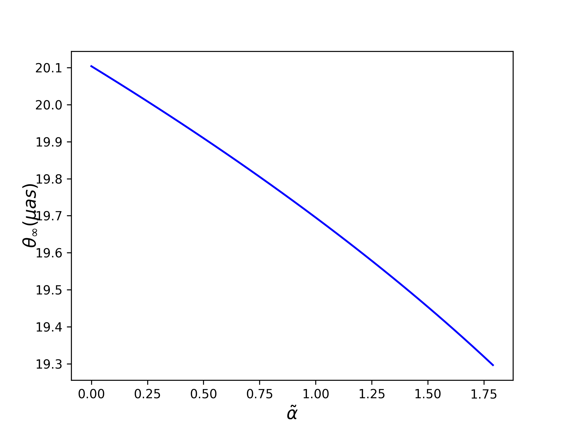
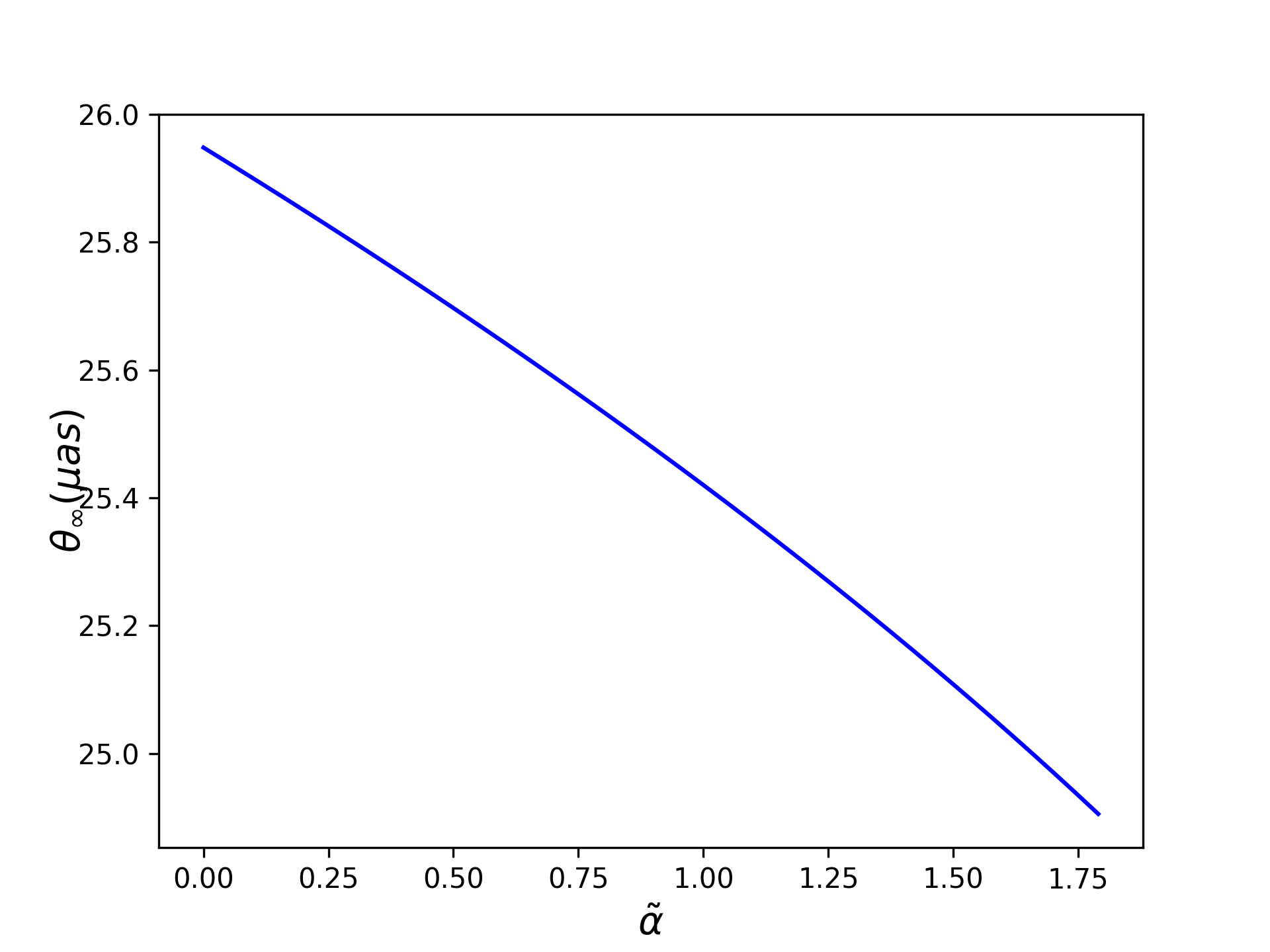
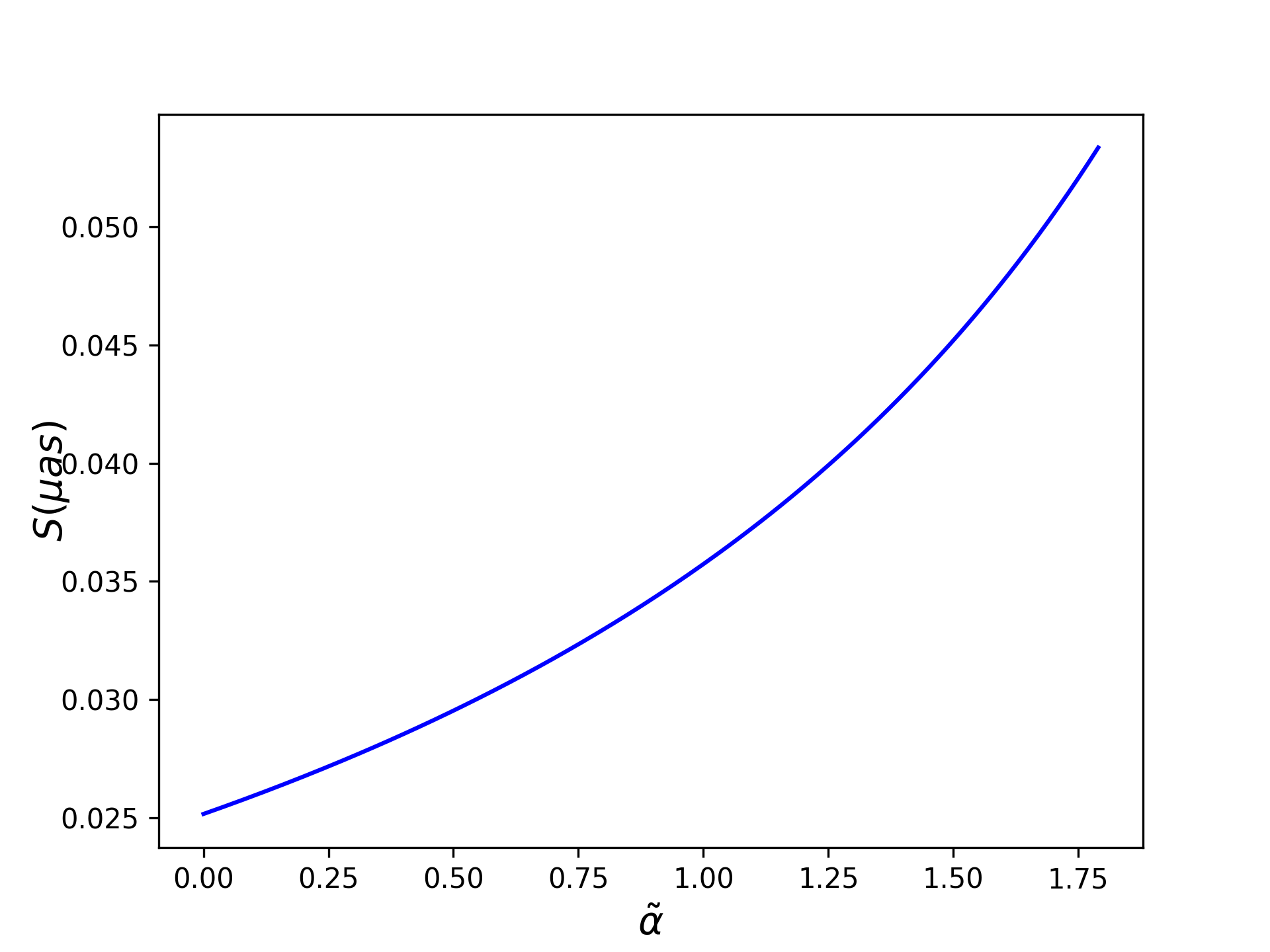
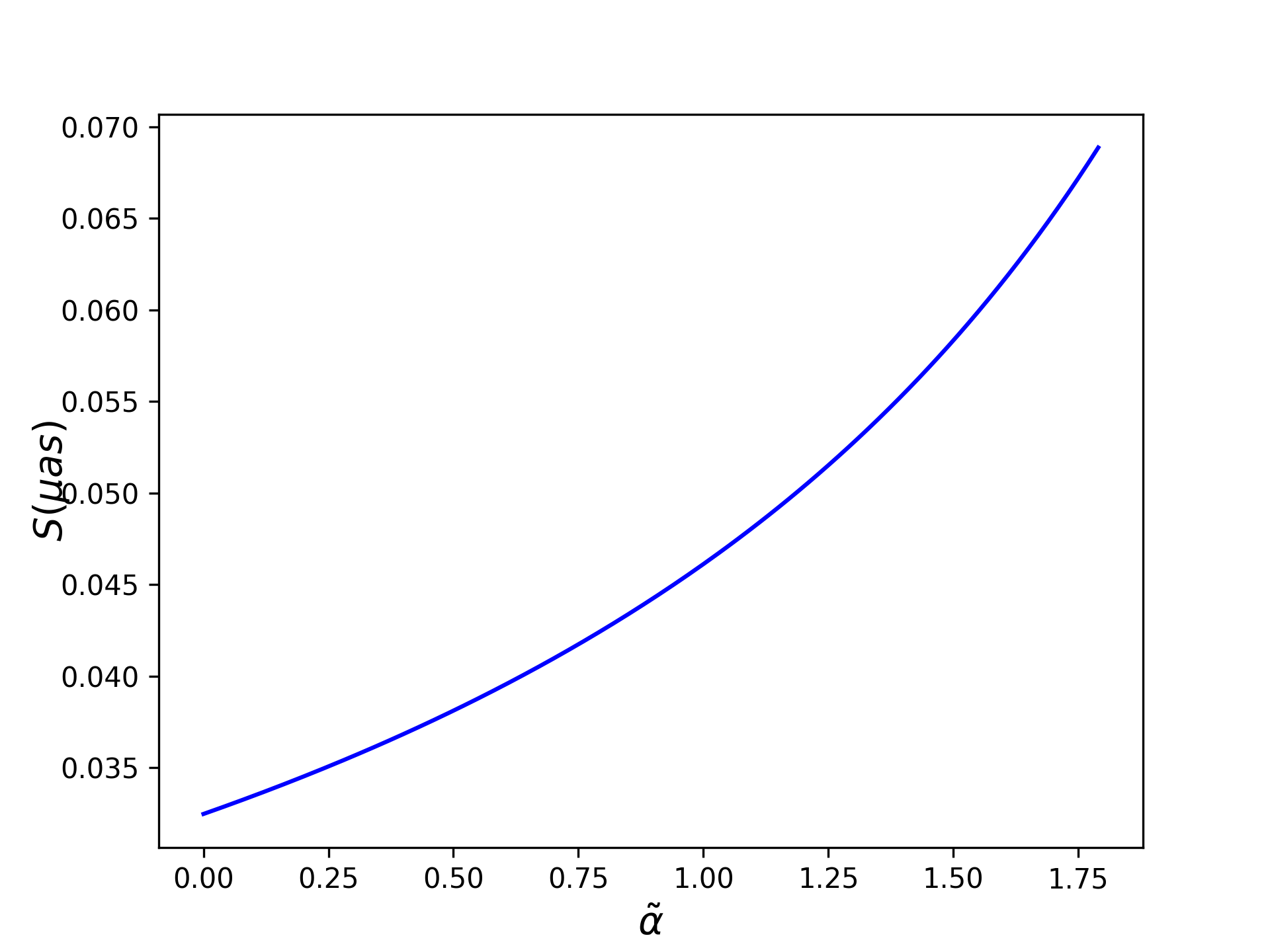
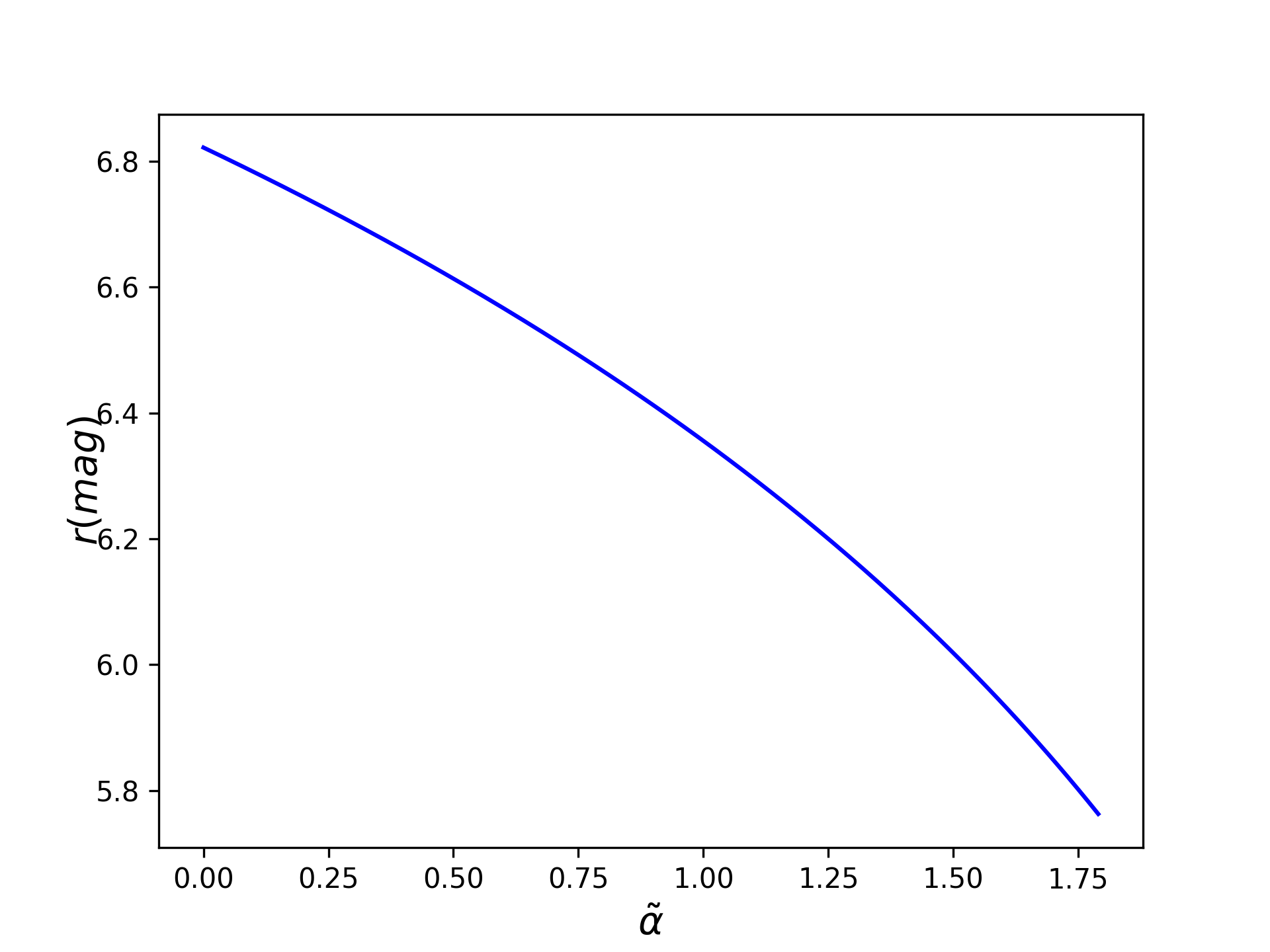
Figure 7: The variation of several interesting observational values for the M87* and SgrA* black holes with changes in the quantum correction parameters, with the left graph representing the M87* black hole and the right graph representing the SgrA* black hole.

	Lensing Coefficients		M87*			SgrA*
$\widetilde{a}$	$\bar{a}$	$\bar{b}$	$\theta_{\infty}(\mu as)$	$s(\mu as)$	$r_{m}$	$\theta_{\infty}(\mu as)$	$s(\mu as)$	$r_{m}$
0.0000	1.0000	-0.4002	20.1042	0.0252	6.8219	25.9482	0.0325	6.8219
0.5000	1.0315	-0.4355	19.9096	0.0295	6.6135	25.6971	0.0382	6.6135
1.0000	1.0733	-0.4919	19.6950	0.0357	6.3557	25.4201	0.0461	6.3557
1.5000	1.1335	-0.5913	19.4534	0.0451	6.0185	25.1082	0.0583	6.0185
1.7000	1.1664	-0.6545	19.3466	0.0505	5.8485	24.9704	0.0652	5.8485

Table 1: Lens system coefficients and observational values of supermassive black holes.

V Weak gravitational lensing in quantum-corrected black holes

In this section, we will explore the impact of quantum correction parameters on the deflection angle of light rays in the weak GL effect of quantum-corrected BHs. We will use the Gauss-Bonnet theorem to calculate the weak deflection angle of light rays in this section. This theorem is the pioneering work of Gibbons and Werner Gibbons:2008rj ; Werner:2012rc . We will calculate the deflection angle of light rays in the weak field limit in quantum-corrected BHs following their method. Here, we assume that the quantum-corrected BH acts as a gravitational lens L located at the coordinate center, with the positions of the observer (O) and the light source (S) as shown in Figure 8. Based on the literature Ishihara:2016vdc ; Ono:2017pie ; Ono:2019hkw , we can define the deflection angle of light rays on the equatorial plane in the weak field approximation

$$\alpha_{D}=\psi_{o}-\psi_{s}+\Phi_{os},$$ (54)

here, $\psi_{o}$ and $\psi_{s}$ correspond to the angles between the line connecting the light source or observer and the lens, respectively. $\Phi_{os}$ represents the angular distance between the observer and the light source. For the convenience of integration, we choose the integration region $D$ of the quadrilateral ${}_{O}^{\infty}\Box_{S}^{\infty}$. At this point, the deflection angle of light is Ono:2017pie

$$\alpha_{D}=-\iint_{D}{K_{o}dS-\int_{o}^{S}{k_{g}d\iota}},$$ (55)

here, $K_{o}$ represents the Gaussian curvature, and $k_{g}$ represents the geodesic curvature. For the quantum-corrected BH (2), the null geodesic behavior $(ds^{2}=0)$, the metric (1) can be obtained

$$dt=\sqrt{\gamma_{ij}dx^{i}dx^{j}}+\rho_{i}dx^{i}.$$ (56)

Here, $\gamma_{ij}$ is the defined three-dimensional Riemannian manifold, and $\rho_{i}dx^{i}$ can be represented as

$$\rho_{i}dx^{i}=-\frac{g_{t\phi}}{g_{tt}}d\phi.$$ (57)

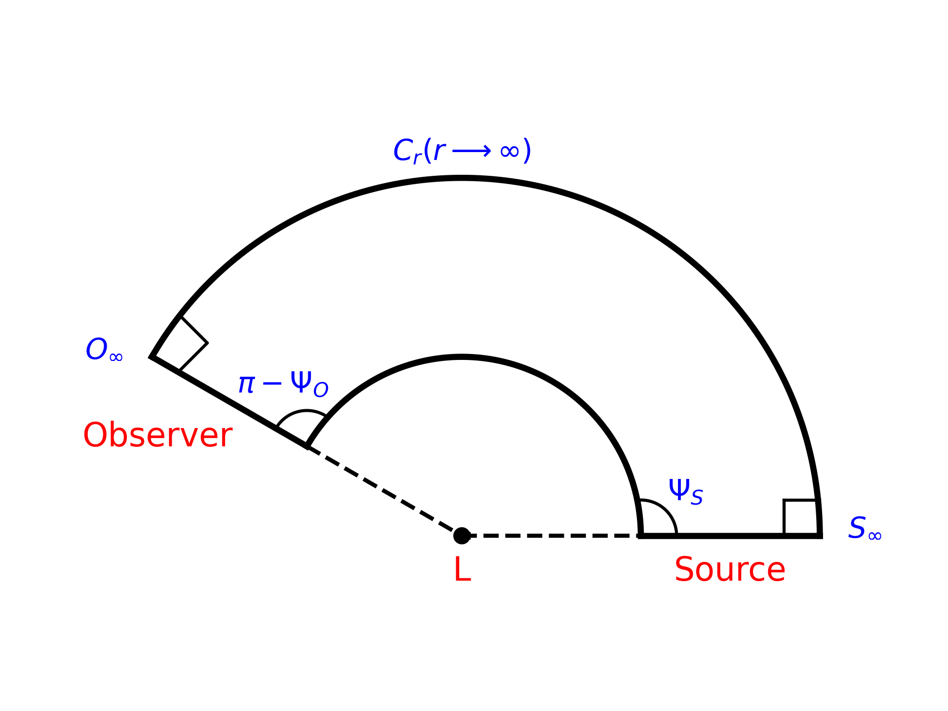
Figure 8: Schematic diagram of a quadrilateral in curved spacetime ${}_{O}^{\infty}\Box_{S}^{\infty}$.

For the metric (1), since the quantum-corrected BH is a static spherically symmetric metric, it follows that $g_{t\phi}=0$, that is, at this time $\rho_{i}dx^{i}=0$, which means the geodesic curvature $k_{g}=0$. At this point, the deflection angle can be rewritten as

$$\alpha_{D}=-\iint_{D}{K_{o}dS}.$$ (58)

When the motion of light is restricted to the equatorial plane $(\theta=\frac{\pi}{2})$, $\gamma_{ij}dx^{i}dx^{j}$ can be rewritten as

$$\gamma_{ij}dx^{i}dx^{j}=\frac{1}{{f(r)}^{2}}dr^{2}+\frac{r^{2}}{f(r)}d\phi^{2}.$$ (59)

At this time, $dS$ can be defined as

$$dS=\sqrt{\gamma}drd\phi.$$ (60)

The Gaussian curvature $K_{o}$ can be defined as Qiao:2022nic ; Werner:2012rc ; Ono:2017pie

$$K_{o} =\frac{1}{\sqrt{\gamma}}\left[\frac{\partial}{\partial\phi}\left(\frac{\sqrt{\gamma}}{\gamma_{rr}}\Gamma_{rr}^{\phi}\right)-\frac{\partial}{\partial r}\left(\frac{\sqrt{\gamma}}{\gamma_{rr}}\Gamma_{r\phi}^{\phi}\right)\right]$$

$$=\frac{1}{2}\ f(r)\frac{d^{2}f(r)}{dr^{2}}-\left(\frac{1}{2}\frac{df(r)}{dr}\right)^{2}.$$ (61)

Here, $\gamma$ is the determinant of equation (59). Substituting the metric (2) of the quantum-corrected BH into equation (61) yields the expression for the Gaussian curvature as

$$K_{o}\approx-\frac{2M}{r^{3}}+\frac{3M^{2}}{r^{4}}+\frac{10\alpha M^{2}}{r^{6}}+O(\alpha M^{3},\alpha^{2}M^{4}),$$ (62)

and

$$dS=\sqrt{\gamma}drd\phi\approx\left(r+3M+\frac{15M^{2}}{2r^{3}}-\frac{3\alpha M^{2}}{2r^{3}}\right)\ drd\phi.$$ (63)

Thus, at this point, the closed integral can be represented as Ono:2017pie

$$\alpha_{D}=-\iint_{D}{K_{o}dS}=\int_{\phi_{s}}^{\phi_{o}}\int_{\infty}^{r_{0}}{K_{o}\sqrt{\gamma}drd\phi},$$ (64)

in the above equation, $r_{0}$ represents the minimum distance of the light ray when approaching the vicinity of a BH. In the weak field approximation, the path of the light ray can be approximated as Crisnejo:2019ril

$$u= \frac{sin\phi}{b}+\frac{M\left(1-cos\phi\right)^{2}}{b^{2}}$$

$$-\frac{M^{2}\left(60\phi cos\phi+3sin3\phi-5sin\phi\right)}{16b^{3}}$$

$$+O(higher-order\,terms),$$ (65)

here, $u=\frac{1}{r}$, where $b$ represents the impact parameter. At this point, integral (64) can be expressed as

$$\alpha_{D}=\int_{\phi_{s}}^{\phi_{o}}\int_{0}^{u}{-\frac{K_{o}\sqrt{\gamma}}{u^{2}}dud\phi}.$$ (66)

In the weak field approximation, we select the range of variation for $\phi$ to be between $-\pi$ and $\pi$, more specifically, $\phi_{o}$ is constrained to $\left|\phi_{o}\right|>\frac{\pi}{2}$, while $\phi_{s}$ is constrained to $\left|\phi_{s}\right|\leq\frac{\pi}{2}$. Since we are dealing with a quantum-corrected BH that is asymptotically flat, we primarily consider the case where the source and the observer are infinitely far from the BH, which does not lose generality, that is, $u_{s}\rightarrow 0$ and $u_{0}\rightarrow 0$. Under these circumstances, we can obtain the following approximation

$$\phi_{s}\rightarrow 0,$$ (67)

$$\phi_{o}\rightarrow\pi.$$ (68)

At this point, the integral (66) can be re-expressed as

$$\alpha_{D}=\int_{0}^{\pi}\int_{0}^{u}{-\frac{K_{o}\sqrt{\gamma}}{u^{2}}dud\phi}.$$ (69)

By substituting formulas (62) and (63) into the above expression, we obtain

$$\alpha_{D} =\int_{0}^{\pi}\int_{0}^{u}{-\frac{K_{o}\sqrt{\gamma}}{u^{2}}dud\phi}$$

$$=\int_{0}^{\pi}\int_{0}^{u}\left(2M+3uM^{2}+6u^{2}M^{3}\right.$$

$$\left.-10\alpha u^{3}M^{2}-15\alpha u^{4}M^{3}\right)dud\phi+O(M^{4})$$

$$\approx\frac{4M}{b}+\frac{15\pi M^{2}}{4b^{2}}-\frac{15{\alpha\pi M}^{2}}{16b^{4}}+\frac{80M^{3}}{3b^{3}}-\frac{96{\alpha M}^{3}}{5b^{5}}+O(M^{4}).$$ (70)

The above formula represents the deflection angle in a quantum-corrected BH. It is easy to see that the quantum correction parameter affects the deflection angle in the weak field approximation (here, the quantum correction parameter mainly reduces the deflection angle of the Schwarzschild BH), and the most significant effects are at the second order and above, $O(M^{2})$. When the quantum correction parameter disappears $(\alpha=0)$, the quantum-corrected BH degenerates into a Schwarzschild BH in the weak field approximation, and the degenerated deflection angle of the quantum-corrected BH is the same as that of the Schwarzschild BH Virbhadra:1999nm ; Crisnejo:2019ril ; Ono:2019hkw , that is

$$\alpha_{D(Schw)}=\frac{4M}{b}+\frac{15\pi M^{2}}{4b^{2}}+\frac{80M^{3}}{3b^{3}}+O(M^{4}).$$ (71)

Just as we analyze the deflection angle in the strong field limit, we adopt dimensionless parameters for nondimensionalization, that is, $\widetilde{b}=\frac{b}{M}$, $\widetilde{\alpha}=\frac{\alpha}{M^{2}}$. At this point, the deflection angle (70) becomes

$$\alpha_{D}=\frac{1}{\widetilde{b}}+\frac{15\pi}{4{\widetilde{b}}^{2}}-\frac{15\widetilde{\alpha}\pi}{16{\widetilde{b}}^{4}}+\frac{80}{3{\widetilde{b}}^{3}}-\frac{96\widetilde{\alpha}}{5{\widetilde{b}}^{5}}+O(\frac{1}{{\widetilde{b}}^{4}}).$$ (72)

To intuitively observe the impact of the quantum correction parameter on the deflection angle in the weak field limit, we define the deviation $\delta\alpha=\alpha_{D(Schw)}-\alpha_{D}$. As shown in Figure 9, when the quantum correction parameter is fixed, the deviation decreases rapidly with the increase of the impact parameter, eventually approaching zero. As expected, the quantum correction parameter has a significant impact on smaller impact parameters (see Figure 9).

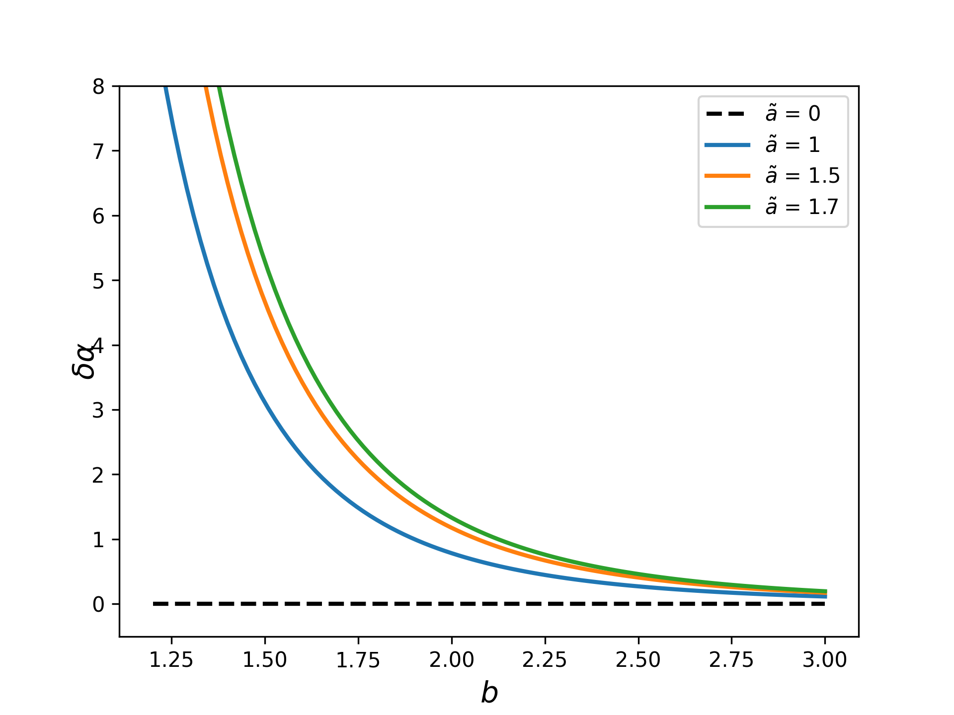
Figure 9: The graph of the deviation $\delta\alpha$ as a function of the impact parameter $b$.

VI Discussion and conclusions

The GL effect, as a powerful astronomical tool, not only plays a key role in solving complex astrophysical problems but also demonstrates great potential in verifying GR and exploring the validity of other modified gravitational theories. Therefore, in this paper, we calculate the lensing effect in a quantum-corrected BH, analyze the impact of the quantum correction parameter $\alpha$ on the lensing coefficients $(\bar{a},\bar{b})$ and the deflection angle. We also assume that the QCBH is a candidate for the supermassive BHs M87* and SgrA*, exploring the influence of the quantum correction parameter $\alpha$ on the image position and the Einstein ring. Our conclusions are as follows:

In the strong field limit, we use the method proposed by Bozza et al. to calculate the deflection angle and corresponding deflection angle coefficients in a quantum-corrected BH. Through numerical analysis, our results show that the lensing coefficient $\bar{a}$ increases with the increase of the quantum correction parameter $\alpha$, while the deflection angle $\alpha_{D}$ and lensing coefficient $\bar{b}$ decrease as the quantum correction parameter $\alpha$ decreases.

In considering the QCBH as a candidate for the supermassive BHs M87* and SgrA*, our conclusions indicate that the image position $\theta_{\infty}$ and the brightness ratio between relativistic images $r_{mag}$ decrease as the quantum correction parameter increases, while the separation $S$ between the images increases with the quantum correction parameter. Moreover, our calculations show that the presence of the quantum correction parameter $\alpha$ results in a smaller Einstein ring for the QCBH compared to the Schwarzschild BH. Although the presence of the quantum correction parameter introduces many differences between the quantum-corrected and Schwarzschild BHs, ur results show that the range of the relativistic image angular position $\theta_{\infty}$ with the quantum correction parameter’s variation is $20.1042\mu as\geq\theta_{\infty}(M87*)\geq 19.3466\mu as$ and $25.9482\mu as\geq\theta_{\infty}(SgrA*)\geq 24.9704\mu as$. that is,the deviation in the angular position of the relativistic images between the quantum-corrected and Schwarzschild BHs does not exceed $1\mu as$ (see Table 1 and Figure 7). In other words, given the current resolution of the EHT, distinguishing between a Schwarzschild BH and a QCBH is challenging. This implies that to further test LQG theories, there is a need to enhance the resolution of the EHT.

In the weak field approximation, our results show that the presence of the quantum correction parameter $\alpha$ has a suppressive effect on the weak deflection angle of the Schwarzschild BH, and this suppression starts from the second order.

In summary, assuming that quantum-corrected BHs are not merely theoretical constructs but actually exist in the universe, our analysis indicates that with the continuous advancement and refinement of astrophysical observational techniques (such as the increasing observational precision of the EHT), using the lensing effect as a verification tool to test the accuracy of LQG theory becomes feasible. By combining theoretical predictions with actual observational data, this provides us with a unique perspective to make an accurate distinction between Schwarzschild black holes under general relativity and quantum-corrected BHs in LQG theory. Furthermore, the application of this method is expected not only to advance our understanding in the field of black hole physics but also to provide crucial insights into unveiling the fundamental physical laws of the universe and deepening our comprehension of LQG theory.

VII acknowledgements

We acknowledge the anonymous referee for a constructive report that has significantly improved this paper. This work was supported by the Special Natural Science Fund of Guizhou University (Grant No.X2022133), the National Natural Science Foundation of China (Grant No. 12365008) and the Guizhou Provincial Basic Research Program (Natural Science) (Grant No. QianKeHeJiChu-ZK[2024]YiBan027) .

References

- (1) B. P. Abbott et al. GW150914: The Advanced LIGO Detectors in the Era of First Discoveries. Phys. Rev. Lett., 116(13):131103, 2016. doi = 10.1103/PhysRevLett.116.131103
- (2) Clifford M. Will. The Confrontation between General Relativity and Experiment. Living Rev. Rel., 17:4, 2014. doi = 10.12942/lrr-2014-4
- (3) Pedro G. Ferreira. Cosmological Tests of Gravity. Ann. Rev. Astron. Astrophys., 57:335–374, 2019. doi = 10.1146/annurev-astro-091918-104423
- (4) Timothy Clifton, Pedro G. Ferreira, Antonio Padilla, and Constantinos Skordis. Modified Gravity and Cosmology. Phys. Rept., 513:1–189, 2012. doi = 10.1016/j.physrep.2012.01.001
- (5) Kazunori Akiyama et al. First M87 Event Horizon Telescope Results. I. The Shadow of the Supermassive Black Hole. Astrophys. J. Lett., 875:L1, 2019. doi = 10.3847/2041-8213/ab0ec7
- (6) Kazunori Akiyama et al. First Sagittarius A* Event Horizon Telescope Results. I. The Shadow of the Supermassive Black Hole in the Center of the Milky Way. Astrophys. J. Lett., 930(2):L12, 2022. doi = 10.3847/2041-8213/ac6674
- (7) S. W. Hawking and R. Penrose. The Singularities of gravitational collapse and cosmology. Proc. Roy. Soc. Lond. A, 314:529–548, 1970. doi = 10.1098/rspa.1970.0021
- (8) Roger Penrose. Gravitational collapse and space-time singularities. Phys. Rev. Lett., 14:57–59, 1965. doi = 10.1103/PhysRevLett.14.57
- (9) Ellery Ames, Håkan Andréasson, and Oliver Rinne. Hoop and weak cosmic censorship conjectures for the axisymmetric Einstein-Vlasov system. Phys. Rev. D, 108(6):064054, 2023. doi = 10.1103/PhysRevD.108.064054
- (10) Min Zhao, Meirong Tang, and Zhaoyi Xu. Testing The Weak Cosmic Censorship Conjecture in Short Haired Black Holes. 2 2024. eprint = 2402.16373
- (11) Liping Meng, Zhaoyi Xu, and Meirong Tang. Exploring the Impact of Coupled Behavior on the Weak Cosmic Censorship Conjecture in Cold Dark Matter-Black Hole Systems. 1 2024. eprint = 2401.11482
- (12) Lai Zhao, Zhaoyi Xu, and Meirong Tang. The Weak Cosmic Censorship Conjecture in Hairy Kerr Black Holes. 1 2024. eprint = 2401.11379
- (13) Meirong Tang and Zhaoyi Xu. Test the weak cosmic censorship conjecture via cold dark matter-black hole and ultralight dark matter-black hole. 11 2023. eprint = 2311.04415
- (14) Liping Meng, Zhaoyi Xu, and Meirong Tang. Test the weak cosmic supervision conjecture in dark matter-black hole system. Eur. Phys. J. C, 83(10):986, 2023. doi = 10.1140/epjc/s10052-023-12163-w
- (15) Jafar Sadeghi, Mohammad Reza Alipour, and Saeed Noori Gashti. Strong cosmic censorship in light of weak gravity conjecture for charged black holes. JHEP, 02:236, 2023. doi = 10.1007/JHEP02(2023)236
- (16) Lai Zhao and Zhaoyi Xu. Destroying the event horizon of a rotating black-bounce black hole. Eur. Phys. J. C, 83(10):938, 2023. doi = 10.1140/epjc/s10052-023-12117-2
- (17) Abhay Ashtekar, Tomasz Pawlowski, and Parampreet Singh. Quantum Nature of the Big Bang: Improved dynamics. Phys. Rev. D, 74:084003, 2006. doi = 10.1103/PhysRevD.74.084003
- (18) Jinsong Yang, Cong Zhang, and Yongge Ma. Shadow and stability of quantum-corrected black holes. Eur. Phys. J. C, 83(7):619, 2023. doi = 10.1140/epjc/s10052-023-11800-8
- (19) Muxin Han, Weiming Huang, and Yongge Ma. Fundamental structure of loop quantum gravity. Int. J. Mod. Phys. D, 16:1397–1474, 2007. doi = 10.1142/S0218271807010894
- (20) Abhay Ashtekar and Jerzy Lewandowski. Background independent quantum gravity: A Status report. Class. Quant. Grav., 21:R53, 2004. doi = 10.1088/0264-9381/21/15/R01
- (21) Alejandro Perez. The Spin Foam Approach to Quantum Gravity. Living Rev. Rel., 16:3, 2013. doi = 10.12942/lrr-2013-3
- (22) Kristina Giesel and Hanno Sahlmann. From Classical To Quantum Gravity: Introduction to Loop Quantum Gravity. PoS, QGQGS2011:002, 2011. doi = 10.22323/1.140.0002
- (23) Thomas Thiemann. Lectures on loop quantum gravity. Lect. Notes Phys., 631:41–135, 2003. doi = 10.1007/978-3-540-45230-0_3
- (24) Abhay Ashtekar, Tomasz Pawlowski, and Parampreet Singh. Quantum nature of the big bang. Phys. Rev. Lett., 96:141301, 2006. doi = 10.1103/PhysRevLett.96.141301
- (25) Abhay Ashtekar, Tomasz Pawlowski, and Parampreet Singh. Quantum Nature of the Big Bang: An Analytical and Numerical Investigation. I. Phys. Rev. D, 73:124038, 2006. doi = 10.1103/PhysRevD.73.124038
- (26) Abhay Ashtekar, Martin Bojowald, and Jerzy Lewandowski. Mathematical structure of loop quantum cosmology. Adv. Theor. Math. Phys., 7(2):233–268, 2003. doi = 10.4310/ATMP.2003.v7.n2.a2
- (27) Theodoros Papanikolaou. Primordial black holes in loop quantum cosmology: the effect on the threshold. Class. Quant. Grav., 40(13):134001, 2023. doi = 10.1088/1361-6382/acd97d
- (28) Ghanashyam Date and Golam Mortuza Hossain. Genericity of big bounce in isotropic loop quantum cosmology. Phys. Rev. Lett., 94:011302, 2005. doi = 10.1103/PhysRevLett.94.011302
- (29) G. V. Vereshchagin. Qualitative approach to semi-classical loop quantum cosmology. JCAP, 07:013, 2004. doi = 10.1088/1475-7516/2004/07/013
- (30) Parampreet Singh and Alexey Toporensky. Big crunch avoidance in K=1 semiclassical loop quantum cosmology. Phys. Rev. D, 69:104008, 2004. doi = 10.1103/PhysRevD.69.104008”,
- (31) Edward Wilson-Ewing. Testing loop quantum cosmology. Comptes Rendus Physique, 18:207–225, 2017. doi = 10.1016/j.crhy.2017.02.004
- (32) Norbert Bodendorfer, Fabio M. Mele, and Johannes Münch. (b,v)-type variables for black to white hole transitions in effective loop quantum gravity. Phys. Lett. B, 819:136390, 2021. doi = 10.1016/j.physletb.2021.136390
- (33) Abhay Ashtekar, Javier Olmedo, and Parampreet Singh. Quantum Transfiguration of Kruskal Black Holes. Phys. Rev. Lett., 121(24):241301, 2018. doi = 10.1103/PhysRevLett.121.241301
- (34) Suddhasattwa Brahma, Che-Yu Chen, and Dong-han Yeom. Testing Loop Quantum Gravity from Observational Consequences of Nonsingular Rotating Black Holes. Phys. Rev. Lett., 126(18):181301, 2021. doi = 10.1103/PhysRevLett.126.181301
- (35) Norbert Bodendorfer, Fabio M. Mele, and Johannes Münch. Mass and Horizon Dirac Observables in Effective Models of Quantum Black-to-White Hole Transition. Class. Quant. Grav., 38(9):095002, 2021. doi = 10.1088/1361-6382/abe05d
- (36) Jerzy Lewandowski, Yongge Ma, Jinsong Yang, and Cong Zhang. Quantum Oppenheimer-Snyder and Swiss Cheese Models. Phys. Rev. Lett., 130(10):101501, 2023. doi = 10.1103/PhysRevLett.130.101501
- (37) Huajie Gong, Shulan Li, Dan Zhang, Guoyang Fu, and Jian-Pin Wu. Quasinormal modes of quantum-corrected black holes. 12 2023. eprint = 2312.17639
- (38) Jing-Peng Ye, Zhi-Qing He, Ai-Xu Zhou, Zi-Yang Huang, and Jia-Hui Huang. Shadows and photon rings of a quantum black hole. Phys. Lett. B, 851:138566, 2024. doi = 10.1016/j.physletb.2024.138566
- (39) Cai-Ying Shao, Cong Zhang, Wei Zhang, and Cheng-Gang Shao. Scalar fields around a loop quantum gravity black hole in de Sitter spacetime: Quasinormal modes, late-time tails and strong cosmic censorship. Phys. Rev. D, 109(6):064012, 2024. doi = 10.1103/PhysRevD.109.064012
- (40) Xiangdong Zhang. Loop Quantum Black Hole. Universe, 9(7):313, 2023. doi = 10.3390/universe9070313
- (41) Kristina Giesel, Muxin Han, Bao-Fei Li, Hongguang Liu, and Parampreet Singh. Spherical symmetric gravitational collapse of a dust cloud: Polymerized dynamics in reduced phase space. Phys. Rev. D, 107(4):044047, 2023. doi = 10.1103/PhysRevD.107.044047
- (42) Sjur Refsdal and H. Bondi. The Gravitational Lens Effect. Monthly Notices of the Royal Astronomical Society, 128(4):295–306, 09 1964. doi = 10.1093/mnras/128.4.295
- (43) Sidney Liebes. Gravitational Lenses. Phys. Rev., 133:B835–B844, 1964. doi = 10.1103/PhysRev.133.B835
- (44) V. Bozza. Gravitational lensing in the strong field limit. Phys. Rev. D, 66:103001, 2002. doi = 10.1103/PhysRevD.66.103001
- (45) K. S. Virbhadra and George F. R. Ellis. Schwarzschild black hole lensing. Phys. Rev. D, 62:084003, 2000. doi = 10.1103/PhysRevD.62.084003
- (46) V. Bozza, S. Capozziello, G. Iovane, and G. Scarpetta. Strong field limit of black hole gravitational lensing. Gen. Rel. Grav., 33:1535–1548, 2001. doi = 10.1023/A:1012292927358
- (47) Naoki Tsukamoto. Deflection angle in the strong deflection limit in a general asymptotically flat, static, spherically symmetric spacetime. Phys. Rev. D, 95(6):064035, 2017. doi = 10.1103/PhysRevD.95.064035
- (48) Yujie Duan, Siyan Lin, and Junji Jia. Deflection and gravitational lensing with finite distance effect in the strong deflection limit in stationary and axisymmetric spacetimes. JCAP, 07:036, 2023. doi = 10.1088/1475-7516/2023/07/036
- (49) Jitendra Kumar, Shafqat Ul Islam, and Sushant G. Ghosh. Strong gravitational lensing by loop quantum gravity motivated rotating black holes and EHT observations. Eur. Phys. J. C, 83(11):1014, 2023. doi = 10.1140/epjc/s10052-023-12205-3
- (50) Saptaswa Ghosh and Arpan Bhattacharyya. Analytical study of gravitational lensing in Kerr-Newman black-bounce spacetime. JCAP, 11:006, 2022. doi = 10.1088/1475-7516/2022/11/006
- (51) Tien Hsieh, Da-Shin Lee, and Chi-Yong Lin. Gravitational time delay effects by Kerr and Kerr-Newman black holes in strong field limits. Phys. Rev. D, 104(10):104013, 2021. doi = 10.1103/PhysRevD.104.104013
- (52) Shafqat Ul Islam and Sushant G. Ghosh. Strong field gravitational lensing by hairy Kerr black holes. Phys. Rev. D, 103(12):124052, 2021. doi = 10.1103/PhysRevD.103.124052
- (53) Tien Hsieh, Da-Shin Lee, and Chi-Yong Lin. Strong gravitational lensing by Kerr and Kerr-Newman black holes. Phys. Rev. D, 103(10):104063, 2021. doi = 10.1103/PhysRevD.103.104063
- (54) Songbai Chen, Yue Liu, and Jiliang Jing. Strong gravitational lensing in a squashed Kaluza-Klein Gödel black hole. Phys. Rev. D, 83:124019, 2011. doi = 10.1103/PhysRevD.83.124019
- (55) Ernesto F. Eiroa and Diego F. Torres. Strong field limit analysis of gravitational retro lensing. Phys. Rev. D, 69:063004, 2004. doi = 10.1103/PhysRevD.69.063004
- (56) Richard Whisker. Strong gravitational lensing by braneworld black holes. Phys. Rev. D, 71:064004, 2005. doi = 10.1103/PhysRevD.71.064004
- (57) Ernesto F. Eiroa. Braneworld black holes as gravitational lenses. Braz. J. Phys., 35:1113–1116, 2005. doi = 10.1590/S0103-97332005000700026
- (58) GuoPing Li, Biao Cao, Zhongwen Feng, and Xiaotao Zu. Strong Gravitational Lensing in a Brane-World Black Hole. Int. J. Theor. Phys., 54(9):3103–3114, 2015. [Erratum: Int.J.Theor.Phys. 54, 3864–3865 (2015)]. doi = 10.1007/s10773-015-2545-y
- (59) Shafqat Ul Islam, Rahul Kumar, and Sushant G. Ghosh. Gravitational lensing by black holes in the Einstein-Gauss-Bonnet gravity. JCAP, 09:030, 2020. doi = 10.1088/1475-7516/2020/09/030
- (60) V. Bozza and L. Mancini. Time delay in black hole gravitational lensing as a distance estimator. Gen. Rel. Grav., 36:435–450, 2004. doi = 10.1023/B:GERG.0000010486.58026.4f
- (61) Rahul Kumar, Sushant G. Ghosh, and Anzhong Wang. Shadow cast and deflection of light by charged rotating regular black holes. Phys. Rev. D, 100(12):124024, 2019. doi = 10.1103/PhysRevD.100.124024
- (62) Jitendra Kumar, Shafqat Ul Islam, and Sushant G. Ghosh. Investigating strong gravitational lensing effects by supermassive black holes with Horndeski gravity. Eur. Phys. J. C, 82(5):443, 2022. doi = 10.1140/epjc/s10052-022-10357-2
- (63) Qi Qi, Yuan Meng, Xi-Jing Wang, and Xiao-Mei Kuang. Gravitational lensing effects of black hole with conformally coupled scalar hair. Eur. Phys. J. C, 83(11):1043, 2023. doi = 10.1140/epjc/s10052-023-12233-z
- (64) Sirachak Panpanich, Supakchai Ponglertsakul, and Lunchakorn Tannukij. Particle motions and Gravitational Lensing in de Rham-Gabadadze-Tolley Massive Gravity Theory. Phys. Rev. D, 100(4):044031, 2019. doi = 10.1103/PhysRevD.100.044031
- (65) Gulmina Zaman Babar, Farruh Atamurotov, Shafqat Ul Islam, and Sushant G. Ghosh. Particle acceleration around rotating Einstein-Born-Infeld black hole and plasma effect on gravitational lensing. Phys. Rev. D, 103(8):084057, 2021. doi = 10.1103/PhysRevD.103.084057
- (66) Xiao-Mei Kuang and Ali Övgün. Strong gravitational lensing and shadow constraint from M87* of slowly rotating Kerr-like black hole. Annals Phys., 447:169147, 2022. doi = 10.1016/j.aop.2022.169147
- (67) David H. Weinberg, Michael J. Mortonson, Daniel J. Eisenstein, Christopher Hirata, Adam G. Riess, and Eduardo Rozo. Observational Probes of Cosmic Acceleration. Phys. Rept., 530:87–255, 2013. doi = 10.1016/j.physrep.2013.05.001
- (68) Antony Lewis and Anthony Challinor. Weak gravitational lensing of the CMB. Phys. Rept., 429:1–65, 2006. doi = 10.1016/j.physrep.2006.03.002
- (69) Jozef Bucko, Sambit K. Giri, and Aurel Schneider. Constraining dark matter decay with cosmic microwave background and weak-lensing shear observations. Astron. Astrophys., 672:A157, 2023. doi = 10.1051/0004-6361/202245562
- (70) Richard Massey, Thomas Kitching, and Johan Richard. The dark matter of gravitational lensing. Rept. Prog. Phys., 73:086901, 2010. doi = 10.1088/0034-4885/73/8/086901
- (71) Mauro Sereno. Weak field limit of Reissner-Nordstrom black hole lensing. Phys. Rev. D, 69:023002, 2004. doi = 10.1103/PhysRevD.69.023002
- (72) Charles R. Keeton and A. O. Petters. Formalism for testing theories of gravity using lensing by compact objects. I. Static, spherically symmetric case. Phys. Rev. D, 72:104006, 2005. doi = 10.1103/PhysRevD.72.104006
- (73) M. C. Werner and A. O. Petters. Magnification relations for Kerr lensing and testing Cosmic Censorship. Phys. Rev. D, 76:064024, 2007. doi = 10.1103/PhysRevD.76.064024
- (74) Mauro Sereno and Fabiana De Luca. Analytical Kerr black hole lensing in the weak deflection limit. Phys. Rev. D, 74:123009, 2006. doi = 10.1103/PhysRevD.74.123009
- (75) G. W. Gibbons and M. C. Werner. Applications of the Gauss-Bonnet theorem to gravitational lensing. Class. Quant. Grav., 25:235009, 2008. doi = 10.1088/0264-9381/25/23/235009
- (76) M. C. Werner. Gravitational lensing in the Kerr-Randers optical geometry. Gen. Rel. Grav., 44:3047–3057, 2012. doi = 10.1007/s10714-012-1458-9
- (77) Asahi Ishihara, Yusuke Suzuki, Toshiaki Ono, Takao Kitamura, and Hideki Asada. Gravitational bending angle of light for finite distance and the Gauss-Bonnet theorem. Phys. Rev. D, 94(8):084015, 2016. doi = 10.1103/PhysRevD.94.084015
- (78) Asahi Ishihara, Yusuke Suzuki, Toshiaki Ono, and Hideki Asada. Finite-distance corrections to the gravitational bending angle of light in the strong deflection limit. Phys. Rev. D, 95(4):044017, 2017. doi = 10.1103/PhysRevD.95.044017
- (79) Toshiaki Ono, Asahi Ishihara, and Hideki Asada. Gravitomagnetic bending angle of light with finite-distance corrections in stationary axisymmetric spacetimes. Phys. Rev. D, 96(10):104037, 2017. doi = 10.1103/PhysRevD.96.104037
- (80) Kimet Jusufi, Marcus C. Werner, Ayan Banerjee, and Ali Övgün. Light Deflection by a Rotating Global Monopole Spacetime. Phys. Rev. D, 95(10):104012, 2017. doi = 10.1103/PhysRevD.95.104012
- (81) Kimet Jusufi, Izzet Sakallı, and Ali Övgün. Effect of Lorentz Symmetry Breaking on the Deflection of Light in a Cosmic String Spacetime. Phys. Rev. D, 96(2):024040, 2017. doi = 10.1103/PhysRevD.96.024040
- (82) Kimet Jusufi and Ali Övgün. Gravitational Lensing by Rotating Wormholes. Phys. Rev. D, 97(2):024042, 2018. doi = 10.1103/PhysRevD.97.024042
- (83) Qi-Ming Fu, Li Zhao, and Yu-Xiao Liu. Weak deflection angle by electrically and magnetically charged black holes from nonlinear electrodynamics. Phys. Rev. D, 104(2):024033, 2021. doi = 10.1103/PhysRevD.104.024033
- (84) Ali Övgün, Kimet Jusufi, and İzzet Sakallı. Exact traversable wormhole solution in bumblebee gravity. Phys. Rev. D, 99(2):024042, 2019. doi = 10.1103/PhysRevD.99.024042
- (85) Wajiha Javed, Sibgha Riaz, Reggie C. Pantig, and Ali Övgün. Weak gravitational lensing in dark matter and plasma mediums for wormhole-like static aether solution. Eur. Phys. J. C, 82(11):1057, 2022. doi = 10.1140/epjc/s10052-022-11030-4
- (86) Xiao-Jun Gao, Xiao-kun Yan, Yihao Yin, and Ya-Peng Hu. Gravitational lensing by a charged spherically symmetric black hole immersed in thin dark matter. Eur. Phys. J. C, 83(4):281, 2023. doi = 10.1140/epjc/s10052-023-11414-0
- (87) Kazunori Akiyama et al. First M87 Event Horizon Telescope Results. II. Array and Instrumentation. Astrophys. J. Lett., 875(1):L2, 2019. doi = 10.3847/2041-8213/ab0c96
- (88) D. Pugliese, H. Quevedo, and R. Ruffini. Circular motion of neutral test particles in Reissner-Nordström spacetime. Phys. Rev. D, 83:024021, 2011. doi = 10.1103/PhysRevD.83.024021
- (89) Qingyu Gan, Peng Wang, Houwen Wu, and Haitang Yang. Photon spheres and spherical accretion image of a hairy black hole. Phys. Rev. D, 104(2):024003, 2021. doi = 10.1103/PhysRevD.104.024003
- (90) Guangzhou Guo, Xin Jiang, Peng Wang, and Houwen Wu. Gravitational lensing by black holes with multiple photon spheres. Phys. Rev. D, 105(12):124064, 2022. doi = 10.1103/PhysRevD.105.124064
- (91) Ghulam Mustafa, Farruh Atamurotov, Ibrar Hussain, Sanjar Shaymatov, and Ali Övgün. Shadows and gravitational weak lensing by the Schwarzschild black hole in the string cloud background with quintessential field*. Chin. Phys. C, 46(12):125107, 2022. doi = 10.1088/1674-1137/ac917f
- (92) S. Chandrasekhar. The Mathematical Theory of Black Holes. Fundam. Theor. Phys., 9:5–26, 1984. doi = 10.1007/978-94-009-6469-3_2
- (93) K. S. Virbhadra, D. Narasimha, and S. M. Chitre. Role of the scalar field in gravitational lensing. Astron. Astrophys., 337:1–8, 1998. eprint = astro-ph/980117
- (94) Qi-Ming Fu and Xin Zhang. Gravitational lensing by a black hole in effective loop quantum gravity. Phys. Rev. D, 105(6):064020, 2022. doi = 10.1103/PhysRevD.105.064020
- (95) Sohan Kumar Jha and Anisur Rahaman. Strong gravitational lensing in hairy Schwarzschild background. Eur. Phys. J. Plus, 138(1):86, 2023. doi = 10.1140/epjp/s13360-023-03650-w
- (96) V. Bozza. A Comparison of approximate gravitational lens equations and a proposal for an improved new one. Phys. Rev. D, 78:103005, 2008. doi = 10.1103/PhysRevD.78.103005
- (97) Albert Einstein. Lens-Like Action of a Star by the Deviation of Light in the Gravitational Field. Science, 84:506–507, 1936. doi = 10.1126/science.84.2188.506
- (98) K. S. Virbhadra and C. R. Keeton. Time delay and magnification centroid due to gravitational lensing by black holes and naked singularities. Phys. Rev. D, 77:124014, 2008. doi = 10.1103/PhysRevD.77.124014
- (99) Kazunori Akiyama et al. First M87 Event Horizon Telescope Results. VI. The Shadow and Mass of the Central Black Hole. Astrophys. J. Lett., 875(1):L6, 2019. doi = 10.3847/2041-8213/ab1141
- (100) Zhuo Chen et al. Consistency of the Infrared Variability of SGR A* over 22 yr. Astrophys. J. Lett., 882(2):L28, 2019. doi = 10.3847/2041-8213/ab3c68
- (101) Toshiaki Ono and Hideki Asada. The effects of finite distance on the gravitational deflection angle of light. Universe, 5(11):218, 2019. doi = 10.3390/universe5110218
- (102) Chen-Kai Qiao and Mi Zhou. Gravitational lensing of Schwarzschild and charged black holes immersed in perfect fluid dark matter halo. JCAP, 12:005, 2023. doi = 10.1088/1475-7516/2023/12/005
- (103) Gabriel Crisnejo, Emanuel Gallo, and Kimet Jusufi. Higher order corrections to deflection angle of massive particles and light rays in plasma media for stationary spacetimes using the Gauss-Bonnet theorem. Phys. Rev. D, 100(10):104045, 2019. doi = 10.1103/PhysRevD.100.104045