Contact processes with quenched disorder
on $\mathbb{Z}^{d}$ and on Erdös-Rényi graphs

Abstract

In real systems impurities and defects play an important role in determining their properties. Here we will consider what probabilists have called the contact process in a random environment and what physicists have more precisely named the contact process with quenched disorder. We will concentrate our efforts on the special case called the random dilution model, in which sites independently and with probability $p$ are active and particles on them give birth at rate $\lambda$, while the other sites are inert and particles on them do not give birth. We show that the resulting inhomogeniety can make dramatic changes in the behavior in the supercritical, subcritical, and critical behavior. In particular, the usual exponential decay of the desnity of particles in the subcritical phase becomes a power law (the Griffiths phase), and polynomial decay at the critical value becomes a power of $\log$.

1 Mathematics of random environments

The first process to be studied in a random environment was

Random walk. In the discrete time case this is a Markov chain $X_{n}$ with transtion probability

$$p(x,x+1)=\alpha_{x}\qquad p(x,x-1)=\beta_{x}=1-\alpha_{x}$$

where the $\alpha_{x}$ are i.i.d. and we suppose for simplicity that $\alpha_{x}\in[\epsilon,1-\epsilon]$. When the environment is fixed $X_{n}$ is a birth and death chain, so we can take advantage of the theory that has been developed for that general class of examples. The first step is to find a harmonic function for the chain, i.e., one that makes $h(X_{n})$ a martingale. For this to hold we must have

$$h(x)=\alpha_{x}h(x+1)+\beta_{x}h(x-1)$$

or rearranging

$$h(x+1)-h(x)=\frac{\beta_{x}}{\alpha_{x}}(h(x)-h(x-1))$$ (1)

Let $\rho_{x}=\beta_{x}/\alpha_{x}$. From the resulting properties of $h$ we can conclude easily that.

Theorem 1.1.

(i) If $E\log(\rho)<0$ then $X_{n}\to\infty$ as $n\to\infty$.

(ii) If $E\log(\rho)>0$ then $X_{n}\to-\infty$ as $n\to\infty$.

(iii) If $E\log(\rho_{x})=0$ then $-\infty=\liminf_{n\to\infty}X_{n}<\limsup_{n\to\infty}X_{n}=\infty$,

so $X_{n}$ is recurrent, i.e., for any $y$ it has $X_{m}=y$ infinitely many times.

To check this note that in case (i), the harmonic function defined in (1) has $h(x)\to\infty$ as $x\to-\infty$ and $h(x)\to 0$ as $x\to\infty$ which implies that $X_{n}\to\infty$ as $n\to\infty$.

To delve further into the properties of $X_{n}$ it is useful to let $T_{m}$ be the time of the first visit to $m$. Theorem (1.16) of Solomon (1975) implies that

Theorem 1.2.

(i) If $E\rho<1$ then

$$\lim_{n\to\infty}T_{n}/n=\frac{1+E(\rho)}{1-E(\rho)}\qquad\lim_{n\to\infty}X_{n}/n=\frac{1-E(\rho)}{1+E(\rho)}$$

(ii) If $(E\rho)^{-1}\leq 1\leq E(\rho^{-1})$ then

$$\lim_{n\to\infty}T_{n}/n=\infty\qquad\lim_{n\to\infty}X_{n}/n=0$$

Kesten, Kozlov, and Spitzer (1975) analyzed the possible behaviors of $X_{n}$ in great detail. They have five conclusions that depend on the size of $\kappa$, but the case $\kappa<1$ is the most relevant to our investigation.

Theorem 1.3.

Suppose that $E\log(\rho)<0$, $E(\rho)<1$, the distribution of $\log(\rho)$ is nonarithmetic, and there is a $\kappa\in(0,1)$ so that $E(\rho^{\kappa})=1$. If $F_{\kappa}$ is the distribution of the one sides stable law with index $\kappa$ then

$$\lim_{n\to\infty}P(n^{-1/\kappa}T_{n}\leq x)=F_{\kappa}(x)\qquad\lim_{n\to\infty}P(t^{-\kappa}X_{t}\leq x)=1-F_{\kappa}(x^{-1/\kappa})$$

In Theorems 1.1 and 1.2 the conclusion holds for almost every enrionment. In Theorem 1.3 the limiting distribution occurs when we average over the environment, so in the language of physics the limit theorem is for the annealed system. The results for RWRE become much different in the quenched setting when we first fix the environment, see the work of Jonathan Peterson and friends (2009, 2013). For much more about RWRE see Zeitouni (2004).

The biased voter model in a random environment (BVRE) can be analyzed using the results developed for RWRE. In the ordinary baised voter model we imagine that there is a war between the two opinions on each $0,1$ edge. The $1$ converts the 0 to 1 at rate $\lambda$ and the $0$ converts the 1 to 0 at rate $\delta$. In the random environment version we consider, $\lambda$ remains constant while a 1 at $x$ is converted to 0 by either neighbor at rate $\delta_{x}$.

To study this process it is convenient to construct it from a family of Poisson processes that is called a graphical representation. For each ordered pair of adjacent sites $(x,y)$ with $x\in\mathbb{Z}$ and $y=x\pm 1$ we have to Poisson processes

• $D^{(x,y)}_{n}$, $n\geq 1$ with rate $\delta_{x}$. At arrival times when $\xi_{t}(x)=1$, $\xi_{t}(y)=0$, $x$ flips to 0.

• $B^{(x,y)}_{n}$, $n\geq 1$ with rate $\lambda$. At arrival times when $\xi_{t}(x)=0$, $\xi_{t}(y)=1$, $x$ flips to 1.

Lemma 1.1.

Let $\xi_{t}^{+}$ be the process starting from $\xi^{+}_{0}=(-\infty,0]\cap\mathbb{Z}$. At any time the state of the process is $(-\infty,r_{t}]$ for some $r_{t}$. If $E\log(\lambda/\delta_{x}<0$ then $r_{t}\to\infty$ with probability 1. If $E\log(\lambda/\delta_{x})>0$ then $r_{t}\to-\infty$ with probability 1.

Proof.

Since the location of the right edge is a Markov chain that, when it moves, jumps from $x$ to $x+1$ with probability $\alpha_{x}=\lambda/(\lambda+\delta_{x}$ and jumps from $x$ to $x-1$ with probability $\beta_{x}=\delta_{x})(\lambda+\delta_{x}$, this follows from Theorem 1.1. ∎

Let $\xi_{t}^{-}$ be the process starting from $\xi^{-}_{0}=[0,\infty)\cap\mathbb{Z}$. At any time the state of the process is $[\ell_{t},\infty)$. Since the edge moves to the left at rate $\lambda$ and to the right at rate $\delta(\ell_{t})$, if $E\log(\lambda/\delta_{x})<0$ then $\ell_{t}\to-\infty$ with probability 1. If $E\log(\lambda/\delta_{x})>0$ then $\ell_{t}\to-\infty$ with probability 1.

The graphical representation allows us to define $\xi^{+}_{t}$, $\xi^{-}_{t}$ and $\xi^{0}_{t}$ on the same space . If we do this then

Lemma 1.2.

$\Omega_{t}=\{\xi^{0}_{t}\neq\emptyset\}=\{\ell_{s}\leq r_{s}\hbox{ for all $0\leq s\leq t$}\}$ and on $\Omega_{t}$ we have $\xi^{0}_{t}=[\ell_{t},r_{t}]$.

This gives us a result from Irene Ferreira’s (1990) thesis at Cornell.

Theorem 1.4.

The BVRE dies out when $E\log(\lambda/\delta(x))>0$, survives with positive probability when $E\log(\lambda/\delta(x))<0$, but $[\ell_{t},r_{t}]$ only grows linearly if $E(\lambda/\delta(x))<1$.

The contact process in a random environment (CPRE) was introduced by Bramson, Durrett, and Schonmann (1991). Each integer is independently designated as bad with probability $p$ and good with probability $1-p$. In this environment we have a contact process in which sites in $\xi_{t}$ are occupied by particle. (i) Particles are born at vacant sites at a rate equal to the number of occupied neighbors. (ii) A particle at $x$ dies at rate $\Delta$ if the site is bad and at rate $\delta\leq\Delta$ if the site is good.

The ordinary one dimensional contact process (physicists call this the “clean” version) starting from a finite set the process grows linearly when it does not die out. The main point of the paper by BDS is to show that the CPRE, like the BVRE and the RWRE, has one threshold for survival of the process and a higher one for linear growth of the set of occupied sites. To state the result let $\zeta^{0}_{t}$ be the ordinary contact process with births at rate 1 and deaths at rate $\delta$, starting with only 0 occupied. Let $\Omega_{\infty}=\{\zeta^{0}_{t}\neq\emptyset\hbox{ for all $t$}\}$ be the event that the process survives. Let

$$\delta_{c}=\sup\{\delta:P_{\delta}(\Omega_{\infty})>0\},\quad r^{0}_{t}=\sup\zeta^{0}_{t},\quad\hbox{and}\quad R^{0}=\sup_{t\geq 0}r^{0}_{t}.$$

By considering the state of the process at the first time $n\in\zeta^{0}_{t}$, it is easy to see that

$$P(R^{0}\geq n+m|R^{0}\geq n)\geq P(R^{0}\geq m)$$

If we let $a_{n}=-\log P(R^{0}\geq n)$ then $a_{n+m}\leq a_{n}+a_{m}$ so

$$a_{n}/n\to\inf_{m\geq 1}a_{m}/m=\gamma^{-}_{\perp}(\delta)$$ (2)

and $P(R^{0}\geq n)\leq\exp(-\gamma^{-}_{\perp}(\delta)n)$. $L^{-}_{\perp}=1/\gamma^{-}_{\perp}$ is the subcrtical spatial correlation length. For the proof of (2) and more on the correlation lengths, see Section 3

Let $\Omega_{\infty}=\{\xi^{0}_{t}\neq\emptyset\hbox{ for all $t$}\}$ and $T_{n}=\inf\{t:n\in\xi_{t}^{0}\}$.

Theorem 1.5.

Suppose $\Delta>\delta_{c}$, $\delta=0$, and let $\mu=\gamma^{-}_{\perp}(\Delta)/\log(1/p)$ where $p=P(\delta_{x}=\Delta)$.

(a) If $\mu<1$ then there is a $c>0$ so that $\rho_{n}/n\to c$ a.s. on $\Omega_{\infty}$.

(b) If $\mu\geq 1$ then $(\log T_{n})/\log n\to\mu$ in probability on $\Omega_{\infty}$.

Here $X_{n}\to a$ in probability on $\Omega_{\infty}$ means that for any $\eta>0$

$$P(|X_{n}-a|>\eta,\Omega_{\infty})\to 0$$

where $P$ is the law for the CPRE,

In words on $\Omega_{\infty}$ the right edge

$$r^{0}_{t}=\sup\xi^{0}_{t}\approx\begin{cases}t/c&\hbox{if $\mu<1$}\\ t^{1/\mu}&\hbox{if $\mu>1$}\end{cases}$$

Since $\delta=0$, if the process ever has a particle on the good environment then $\xi^{0}_{t}$ survives. To explain the result note that the longest interval of $\Delta$’s in $[1,n]$ is, by Lemma 5.1

$$\sim(\log n)/\log(1/p).$$

The time it takes the CPRE to cross this bad interval for the first time is

$$\approx\exp[\gamma^{-}_{\perp}(\Delta)\log n/\log(1/p)]=n^{\mu}$$

so if $\mu>1$ the CPRE does not spread linearly.

Theorem 1.5 provides upper bounds on the rate of growth when $\delta>0$. To prove the contact process has two phase transitions it is enough to shwo

Theorem 1.6.

Suppose $p=P(\delta_{x}=\Delta)<1$. There is a $\delta_{0}(\Delta,p)>0$ so that if $\delta<\delta_{0}(\Delta,p)$ then the CPRE survivies. That is, for almost every envirnment

$$P^{e}(\xi^{0}_{t}\neq\emptyset\hbox{ for all $t$})>0$$

Here $e=\{\delta_{x}:x\in\mathbb{Z}\}$ and $P^{e}$ is the probability law of the contact process in the fixed environment $e$. Cafiero, Gabrielli, and Muñoz (1998) have verified “the presence of the sub-linear regime predicted by Bramson, Durret, and Schnmann.” We refer the reader to the paper for ideas about a non-Markovian representation that is the key to their analysis.

There are a number of other results for CPRE. Liggett (1992) considered the inhomogeneous contact process in which the recovery rate at $k$ is $\delta(k)$, births from $k-1\to k$ occur at rate $\lambda(k)$ and from $k+1\to k$ at rate $\rho(k)$. Suppose that the rates are independent, the $\delta(k)$ have a common the distribution and the birth rates $\lambda(k)$ and $\rho(k)$ have a common distribution. The next result has surprisingly explicit and simple conditions

Theorem 1.7.

Let $R=\delta(\lambda+\rho+\delta)/\lambda\rho$ Then the process survives if

$$ER<1$$

The right edge $r_{t}$ of the process starting from 1’s on the nonpositive integers and 0 otherwise has $\limsup r_{t}=\infty$ if

$$E\log R<0$$

Jensen’s inequality implies $\log ER<E\log R$ so the second condition implies the first. In his paper Liggett conjectures that $E\log R<0$ implies survival while $ER<1$ implies that $r_{t}/t\to\alpha>0$. Liggett also gives results for periodic environments. The proofs are based on the powerful but diificult methods that Holley and Liggett (1978) used to prove that the nearest neighbor contact process in $d=1$ has $\lambda_{c}\leq 2$.

Newman and Volchan (1996) considered the one-dimensional contact process in a random environment in which the recovery rates at a site are i.i.d. positive random variables $\delta(x)$ bounded above, while the infection rate is $\epsilon$. They showed that the condtion

$$uP(-\log\delta(x)>u)\to\infty\quad\hbox{as $u\to\infty$}$$

implies that the process survives for all $\epsilon>0$. Much less is known in higher dimensions but Klein (1994) has given a condition that guarantees extinction of the process on $\mathbb{Z}^{d}$.

An interesting, but difficult, open problem is to show

Conjecture. In $d\geq 2$ CPRE expands linearly when it does not die out.

Intuitively this holds because the process is not forced to go through bad regions, but can go around them. The conjecture has been confirmed by simulations of Moreira and Dickman (1996), see page R3093.

How might one prove this? The Bezuidenhout and Grimmett (1990) argument shows that if the ordinary contact process does not die out then for any $\epsilon>0$ it dominates an $M$-dependent oriented percolation (with $M$ independent of $\epsilon$) in which sites are open with probability $1-\epsilon$. If this result could be generalized to the CPRE (and that is a big IF) then the desired result would follow. See Section I.2 of Liggett’s (1999) book for a nicely written version of their argument. Garret and Marchand (2012) have proved a “shape theorem” for the asymptotic behavior of two-dimensonal CPRE but they assumed that all of the environments are supercritical

1.1 Results from the physics literature

Physicists tell us, see e.g., Janssen (1981), that all systems exhibiting a continuous transition into a unique absorbing state, without any any other extra symmetry or conservation laws, belong to the same universality class, namely that of the contact process, and its discrete time version directed percolation (DP), which can be of the site or bond variety). A consequence of this is that the critical exponents of these systems agree and that the they take their mean-field values above the critical dimension $d_{c}=4$.

Kinzel (1985), who was inspired at least in part by Wolfram’s (1983) work on cellular automata, asked if impurities or other forms of disorder changed the critical exponents of DP-systems This question was investigated by Noest in (1986), who phrased his investigation in terms of stochastic cellular automata (SCA) in $D+1$ dimensional space-time satisfying

$$P(s_{i}(t+1)=1)=F_{i}\left(\sum_{j}c_{ij}s_{j}(t)\right)$$ (3)

with $F_{i}(x)=0$ for $x\leq 0$, $0<F_{i}(x)<1$ when $x>0$, and the site updates are done independently. Here we will take $c_{ij}=c$ when $i$ and $j$ are nearest neighbors so the lattice is not random.

Bond percolation is obtained by setting

$$F_{i}(x)=1-\exp(-rx)\quad\hbox{ for $x>0$.}$$ (4)

To check this note that if $s_{j}(t)=1$ for $k$ neighbors of $i$ then

$$P(s_{i}(t+1)=0)=\exp(-rck)\equiv q^{k}$$

so bonds are closed with probability $q=\exp(-rc)$.

Site percolation, also known as the threshold-1 contact process, is obtained by setting

$$F_{i}(x)=cr\quad\hbox{ for $x>0$.}$$ (5)

Note that $cr$ is a constant independent of $x$

Spatial disorder is introduced by letting the $F_{i}$ depend randomly on $i$ or in the two concrete examples, taking the $r_{i}$ to be i.i.d. In this case we call the disorder quenched since randomness is generated initially and we study what occurs for one fixed realization.To quote Noest (1986)

The first question is whether even small spatial disorder is compatible with theunivesality class of DP. An argument in the style of A.B. Harris (1974) shows that this is not the case. Assume that there was a transition with the normal exponents and let the disorder, parameterized by $r$, couple smoothly to the critical value $c^{*}$ of some global SCA rule parameter $c$. Because of the time invariant rules, the fluctuations $\sigma(r)\sim(c-c^{*})$ that affect the large space time clusters depend only on their spatial correlation length $L_{s}\sim(c-c^{*})^{-\nu_{\perp}}$. Thus

$$\sigma(r)\sim(c-c^{*})\sim L_{s}^{-D/2}\sim(c-c^{*})^{-\nu_{\perp}D/2}$$

Self-consistency demands that the fluctuations go to zero faster than $c-c^{*}$ near criticality and so we should have $D\nu_{\perp}>2$.

Here and other excerpts that follow, it is not an exact quote since we have changed notation and some terminology, but we think it faithfully reproduces the ideas in the original.

The correlation length and its critical exponent $\nu_{\perp}$ will be defined in Section 3. The inequality $D\nu_{\perp}>2$ is the Harris criterion for the system to not be changed by randomness. We will return to it in the open problems in Section 2.6. Numerical values for critical exponents for the DP universality class given in Henrischen (2000) suggest that the critical exponents are changed in $d<4$.

$d$	$1$	$2$	$3$	$\geq 4$
$\nu_{\perp}$	1.097	0.73	0.58	1/2

We will now introduced a simple special case that will be our main focus here. In dimensions $D>1$ it is possible to set $r_{i}=1$ with probability $p$ and $=0$ with probability $1-p$. This is called the random dilution form of the model and is the version we will concentrate on. There is a probability $p^{*}$ so that when $p\leq p^{*}$ the network of cells and edges does not form a percolating cluster. On such a network, the existence of a nontrivial stationary distribution for the process is not possible. Noest (1986) has drawn the picture of the phase diagram for a random dllution model that we repoduce in Figure 1

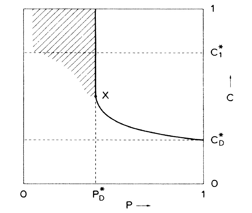
Figure 1: Phase diagram in $D>1$ for randomly diluted site percolation as a function of the dilution probability $p$ and the birth probability which he denotes by $c$.

A second more recent set of results in the physics literature concerns the quenched contact process on Erdös-Rényi graphs. See e.g., Muñoz, Juhász, Castellano, and Ódor (2010). Each site in the graph is independently assigned a birth rate, which is $\lambda$ with probability $p=1-q$, and $r\lambda$ with probability $q$. Again, we will restrict our attention to the case $r=0$. the random dilution model. Juhász, Ódor, Castellano and Muñoz (2012) have derived the phase diagram which we have redrawn in Figure 2.

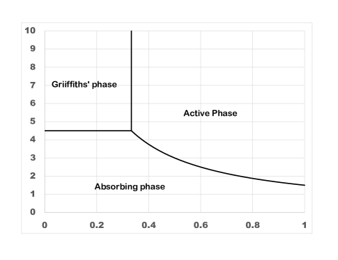
Figure 2: Phase diagram of the random dilution model on an Erdös-Rényi graph with mean degree $\mu=3$, as a function of the fraction of active nodes $p$ and birth rate $\lambda$ and The percolation threshold is $p^{*}=1/3$.

Understanding the phase diagrams in the two Figures will be the main goal of this paper. We will concentrate on four main features.

Supercritical behavior. In $D>1$ and on Erdös-Rényi graphs the critical value remains bounded as the fraction of active sites decreases to the critical value. Intuitively this occurs because whenever there is percolation in either of these two settings then there is a copy of $\mathbb{Z}$ contained in the cluster, so as shown in Figure 1 the multicrtical point $X\leq c^{*}_{1}$, the critical value in one dimension.

The Griffiths phase is labeled in Figure 2. It is the striped region in the Figure 1. Griffiths’ (1969) paper concerned the randomly diluted Ising model and showed that the magnetization fails to be analytic function of the external field $h$ when $h=0$ for a range of temperatures above the critical temperature (which is the subcritical phase of the Ising model). In the case of the contact process (or oriented percolation) the phrase refers to the fact that in the subcritical region decay to the empty state occurs at a power law rate rather than the usual exponential rate. Intuitively, all percolation clusters are finite with a size distribution that has an exponential tail. However the contact process survives for a time that grows exponentially in the size of the cluster so if we start with all sites in state 1 then the density decays to 0 at rate $t^{-\beta(p)}$ with $\beta(p)\to 0$ as $p\uparrow p^{*}$.

Behavior on the critical line $p=p^{*}$ has been studied by Moreira and Dickman (1996) and their mirror image twins Dickman and Moreira (1997). They have found a number of properties of the QCP that are radically different from the homogeneous contact process. One that we can give a rigorous explanation for is the fact that when $p=p^{*}$ the probability of surviving until time $t$, $P(t)\approx 1/(\log t)^{a}$. The intuition is similar to the explanation of the Griffiths’ phse but now the largest cluster sizes are $O(n^{\alpha})$ so the survival time is $\exp(\gamma n^{\alpha})$.

Behavior on the critical curve $\lambda_{c}(p)$, $p>p_{c}$ when $p$ is fixed and $\lambda$ varies is interesting but little is known rigorously. Having heard the claim that critical exponents are constant in the DP universality class, the reader may be surprised to learn that the critical exponents vary along the critical curve. Simulations of Moreira and Dickman (1996) have shown, see Table 1 on page R3091, that if a fraction $x$ of sites are removed in $D=2$ then the critical value $\lambda_{c}(1-x)$ and the critical value for the equilbrium density are (recall that the critical value for site percolation is 0.5927)

$x$	0	0.02	0.05	0.1	0.2	0.3	0.35
$\lambda_{c}$	1.6488	1.6850	1.7409	1.8464	2.1080	2.470	2.719
$\beta$	0.586	0.566	0.79	0.89	0.99	1.07	1.01

It is hard to think about the situation when $x\to 1-p_{c}$, but based on the table and discussion in their papers it is tempting to conjecture that $\beta\to 1$.

If we start with an Erdös-Rényi($N,\mu/N$) graph and delete a fraction $x=1-p$ of the edges we end up with a Erdös-Rényi($N,p\mu/N$) graph. If we delete a fraction $x=1-p$ of the vertices then we end up with a Erdös-Rényi($pN,\mu/N$) graph, which is the same thing except with $M=Np$ vertices. This says that in the Erdös-Rényi case we can understand the critical curve if we look at Erdös-Rényi($N,\lambda/N$) with $\lambda\geq 1$ but in this case the critical exponents are constant.

2 New Rigorous Results

To describe our contributions to the understanding of the behavior of the quenched contact process, we need to first recall a result of Durrett and Schonmann (1988) that will be stated formally in Theorem 3.2: the contact process on $[1,L]$ starting from all sites occupied survives for time $\sigma_{L}$ where

$$(1/L)\log\sigma_{L}\to\gamma_{2}(\lambda)$$ (6)

The same result, with different constants, holds for oriented bond and site percolation, and presumably for all members of the DP universality class.

2.1 Griffiths phase in $D=1$

In contrast to the work of Bramson, Durrett, and Schonmann (1991), we consider the contact process in a random environment in which the death rate is always 1, while the rate of births from $i$ are i.i.d. random variables $\lambda_{i}$. To simplify things, we explore the subcritical region in the random dilution version of the model, in which sites are active with probability $p$ and have $\lambda_{i}=\lambda$ or inert with probability $1-p$ and have $\lambda_{i}=0$. The critical value for percolation in $D=1$ is $p^{*}=1$, but that is not a problem, since we are only interested in the subcritical phase.

For ease of exposition we state our rigorous result before the result of Noest (1988)

Theorem 2.1.

Suppose $p<1$, $\lambda>\lambda_{c}(\mathbb{Z})$, and $\delta>0$. The randomly dliuted contact process on $[1,N]$ starting from all sites occupied survives for time

$$\sigma_{N}\geq N^{(1-\delta)\gamma_{2}(\lambda)/\log(1/p)}\quad\hbox{for large $N$}.$$ (7)

Note that the power of $N$ tends to $\infty$ as $p\uparrow 1$. The proof is easy: straightforward computations, see Lemma 5.1, show that the largest interval of active sites in $[1,N]$,

$$L(p)\sim\log N/\log(1/p).$$

Then we use the result for the contact process on a finite set given in (6). It should be possible to show that replacing $(1-\delta)$ by $(1+\delta)$ in (7) gives an upper bound on the survival time. However to do this we would have to consider the survivial times on all of the intervals of active sites and bound the maximum survival time. Since the lower bound on the survival time is the more interesting result, we leave this more technical computation as an exercise for a reader.

Noest (1998) studied oriented site percolation. Using the notation introduced in Section 1.1, the $r_{i}$ are i.i.d. with $r_{i}=1$ with probability $p$ and 0 otherwise. We have changed the probability sites are open from $c$ to $\theta$ in the definition in (5), since there are already too many things called $c$. Noest begins with observation that the probability a string of length $n$ sites has not reached the empty state by time $t$

$$P(\sigma_{n}>t)=\exp(-t/T_{n})\quad\hbox{where}\quad T_{n}\sim\exp(a(\theta)n)$$

Here $a(\theta)=\gamma_{2}(\theta)$ is the constant in Theorem 3.2 for oriented site percolation. After taking into account the distribution of the lengths of intervals of active sites, he arrives at Theorem 2.2. See Section 5 for details of his proof.

Theorem 2.2.

The fraction of occupied sites at time $u(t)$ satisfies

$$u(t)=(at/b)^{-b/a}\log(at/b)$$ (8)

where $a=\gamma_{2}(\theta)$, and $b=\log(1/p)$.

To connect with (7), note that if we forget about the log factor and the constants then $u(t)=1/N$ (and there are $O(1)$ occupied sites) when

$$t=N^{a/b}=N^{\gamma_{2}(\theta)/\log(1/p)}$$ (9)

2.2 Percolating regime on Erdös-Rényi graphs

When the mean degree of an Erdös-Rényi graph is $\mu>1$ there is a giant component. Ajtai, Komlos, and Szemeredi (1981) were among the first to prove the surprising fact that when $\mu>1$ there is a path with length $O(n)$. Using depth-first search (DFS), Krivelevich and Sudakov (2012) have given a simple proof of this result and Enriquez, Faraud, and Ménard (2017) have proved a result with a sharp constant.

Lemma 2.1.

There is a function $\kappa:(1,\infty)\to(0,1)$ so that the Erdös-Rényi random graph with mean degree $\mu$ contains a path of length at least $\kappa(\mu)N$.

The existence of a path of length $\geq\kappa(\mu)N$ in combination with Theorem 3.2 implies that

Theorem 2.3.

Suppose $\nu=\mu p>1$, $\lambda>\lambda_{c}(\mathbb{Z})$, and $\delta>0$. The randomly diluted contact process on Erdös-Rényi$(N,\mu/N)$ started from all sites occupied survives for time

$$\sigma_{N}\geq\exp((1-\delta)\gamma_{2}(\lambda)\kappa(\mu)N)\qquad\hbox{ for large $N$}.$$

Thus we have demonstrated the phenomenon shown in Figures 1 and 2: the critical birth rate $\lambda$ for long term survival does not $\to\infty$ as $\nu\downarrow 1$.

2.3 Griffiths phase on Erdös-Rényi graphs

The methodof proof is the same as for the result Noest (1988) but, as we will explain, the gap between the physics result and the rigorous one is larger for Erdös-Rényi graphs. We begin by giving the argument from Section II.C of Juhász et al (2012).

The network of active nodes is fragmented and consists of finite clusters whose distribution is given by

$$P(s)\sim\frac{1}{\nu\sqrt{2\pi}}s^{-3/2}e^{-s\alpha(\nu)}\quad\hbox{where $\alpha(\nu)=\nu-1-\ln(\nu)$}$$ (10)

and $\nu=\mu p$ is the average number of edges per vertex in the reduced graph. The long-time decay of the fraction of occupied sites $u(t)$ can be written as the following convolution integral

$$u(t)\sim\int ds\,sP(s)\exp(-t/\tau(s))$$ (11)

where the characteristic decay time $\tau(s)$ of a region of size $s$ grows exponentially (Arrhenius law) with the cluster size

$$\tau(s)=\exp(A(\lambda)s)$$ (12)

and $A(\lambda)$ does not depend on $s$.

Using a saddle-point approximation, see Section 6 for details, one obtains

Theorem 2.4.

The fraction of occupied sites

$$u(t)\sim t^{-\theta(\nu,\lambda)}\quad\hbox{where}\quad\theta(\nu,\lambda)=-\alpha(\nu)/A(\lambda)$$

Again to convert the density result into a survival time we note that $u(t)=1/N$ when

$$t=N^{A(\lambda)/\alpha(\nu)}$$ (13)

To begin to prove our rigorous lower bound on the survival time we note that if we start with Erdös-Rényi$(N,\mu/N)$ and we delete a fraction $1-p$ of the sites then the result is Erdös-Rényi$(Np,\mu/N)$. Let $\nu=\mu p$. Lemma 6.1 shows that as $N\to\infty$ the longest path $\sim(\log N)/\log(1/\nu)$. Using Theorem 3.2 now gives

Theorem 2.5.

Suppose $\nu=\mu p>1$, $\lambda>\lambda_{c}(\mathbb{Z})$, and $\delta>0$. The randomly diluted contact process on Erdös-Rényi$(N,\mu/N)$ starting from all sites occupied survives for time

$$\sigma_{N}\geq N^{(1-\delta)\gamma_{2}(\lambda)/\log(1/\nu)}\qquad\hbox{for large $N$.}$$ (14)

To compare (13) and (14) we note that the assertion that $\tau(s)=\exp(A(\lambda)s)$ where $A(\lambda)$ does not depend on $s$ implies that in computing the logarithm of the survival time of the contact process on a finite cluster, only the size matters, a fact we call the Only Size Matters hypothesis. If this was true (and in Section 6 we will show that it is not) then we would have $A(\lambda)=\gamma_{2}(\lambda)$, the survival time on an interval.

Of course even if the constants were equal then there is the difference in the predicted survival time since the physics result uses the largest cluster while the rigorous result uses a long path. Corollary 5.11 of Bollobás (2001) the largest cluster in graph with $n$ vertices

$$=\frac{1}{\alpha(\nu)}\left(\log n-\left(\frac{5}{2}+o(1)\right)\log\log n\right).$$

In constrast Lemma 6.1 shows that there are paths of length $\geq(1-\delta)\log(1/\nu)$. To compare the two sizes we note that if $\nu=1-\epsilon$ then

$$\log(\nu)=-\epsilon-\frac{\epsilon^{2}}{2}-\frac{\epsilon^{3}}{3}\ldots$$

so $\alpha(\nu)=\log(1-\epsilon)-\epsilon\sim\epsilon^{2}/2$.

2.4 Results in two dimensions

We start with $\mathbb{Z}^{2}$ (or $[1,L]^{2}$ with $L=N^{1/2}$) with edges to nearest neighbors and do bond dilution, where we keep edges with probability $p$, and each site $x$ gives birth across (unoriented) edges $\{x,y\}$ at rate $\lambda$.

2.4.1 Percolating regime

One important reason for deleting edges is that in two dimensional bond percolation we are able to exploit planar graph duality between percolation on $\mathbb{Z}^{2}$ and on a dual graph described in Section 7. Using the duality and some well-known facts about sponge crossings we are able to show that with high probability we have a path of length $\geq\kappa_{2}(p)N/\log N$. The existence of such a path in combination with Theorem 3.2 implies that

Theorem 2.6.

Suppose $p>1/2$, $\lambda>\lambda_{c}(\mathbb{Z})$, and $\delta>0$. The nearest neighbor contact process with randomly deleted edges on $\mathbb{L}^{2}\cap[0,N^{1/2}]^{2}$ starting from all sites occupied survives for time

$$\sigma_{N}\geq\exp(\gamma_{2}(\lambda)\kappa_{2}(p)N/\log N)\qquad\hbox{when $N$ is large.}$$

This falls short of the gold standard of survival for time $\exp(cN)$ but if the grid is $100\times 100$ this gives survival for a time longer than any possible simulation.

2.4.2 Griffiths phase

As with one dimensional systems and Erdös-Rényi graphs, we establish the long time persistence in the Griffiths phase by showing the existence of paths of length $O(\log n)$. Thanks to a result of Grimmett (1981) given in Lemma 7.2 which proves the existence of paths of length $\beta_{2}(p)\log n$ in subcritical two-dimensional percolation this is easy

Theorem 2.7.

Suppose $p>1/2$, $\lambda>\lambda_{c}(\mathbb{Z})$, and $\delta>0$. The nearest neighbor contact process with randomly deleted edges on $\mathbb{L}^{2}\cap[0,N^{1/2}]^{2}$ starting from all sites occupied survives for time

$$\sigma_{N}\geq N^{(1-\delta)\beta_{2}(p)\gamma_{2}(\lambda)}\qquad\hbox{for large $N$.}$$ (15)

2.5 On the critical line for Erdös-Rényi and in $D=2$

In each setting we will show that the longest path is $O(N^{\alpha})$ so using Theorem 3.2 the system survives for time $\geq\exp(\gamma_{2}n^{\alpha})$. Computing as we have several times before if $u(t)=1/(\log t)^{1/\alpha}$ then $u(t)=1/n$ when

$$t=\exp(N^{\alpha}).$$

Proof for the Erdös-Rényi graph. We claim that at criticality the longest path will be $O(N^{1/3})$. To argue this informally, it is known that the largest cluster at criticality has $O(N^{2/3})$ vertices. Critical clusters are like critical branching processes. A critical branching process that survives for time $T$ has $O(T^{2})$ individuals, so skipping more than a few steps the longest path should be $O(N^{1/3})$. For a rigorous proof see Addario-Berry, Broutin, and Goldschmidt (2009,2010), who show that critical Erdös-Rényi clusters rescaled by $n^{-1/3}$ converge to a sequence of compact metric spaces,      

Proof for two dimensions. At criticality crossings of an $L\times L$ box have probability $\approx 1/2$, so taking $L=N^{1/2}$ we see that the longest path has length $\geq cN^{1/2}$ with probability $\geq 1/2$.. To argue that we have a path of this length with high probability, we divide the $L\times L$ square into $k^{2}$, $L/k\times L/k$ squares and note that the probability they all fail to have crossings is $\exp(-(\log 2)k^{2})$.

2.6 Open problems

1. In the random dilution model if we fix $p>p^{*}$ and vary $\lambda$ then there is a phase transition at $\lambda_{c}(p)$. Numerical results suggest that the critical exponents vary as a function of $p$ and the power of log decay of the density holds at the critical value $\lambda_{c}(p)$. See Dickman and Moreira (1997).

2. Understanding the behavior of two dimensional contact process with two birth rates $\lambda$ and $r\lambda$ is difficult, since the critical value no longer coincides with the onset of percolation. See Vojta and Dickison (2005) and Vojta, Farquahr, and Mast (2009) where the intriguing notation of an infiinite randomness fixed point is discussed. In both papers this is discussed in Section II.C.

3. There are a number of verbal arguments for the Harris criterion. See page 10 of Vojta’s (2006) or pages 1686–1687 A.B. Harris’ (1974) paper for his original proof. It would be nice to have a mathematical argument in the style of Kesten’s (1987) derivation of scsling relations for percolation. There is a rigorous proof by Chayes, Chayes, Fisher, and Spencer (1986), but it uses finite size scaling variables, which are are difficult (for me at least) to connect that argument with the properties of the QCP.

3 Correlation lengths and survival times

Our two goals in this section are (i) to define correlation length and (ii) state results about the survival time of the contact process on $[1,N]$. The same results can be proved for oriented percolaiton. To formulate our definitions, we need to prove that certain limits exist, which is done using what is commnly known as supermultiplicativity. Suppose $A_{n}$ are events with

$$P(A_{n+m})\geq P(A_{n})P(A_{m})$$

If we set $a_{n}=-\log P(A_{n})$ then the $a_{n}$ are subadditive

$$a_{n+m}\leq a_{n}+a_{m}$$

A standard argument, see (6.4.2) in Durrett (2019) shows that

$$a_{n}/n\to\inf_{m\geq 1}a_{m}/m\equiv\gamma$$ (16)

and hence we have $P(A_{n})\leq e^{-\gamma n}$

We need to define correlation lengths in space and time for subcritical and supercritical contact processes. Here we follow Durrett, Schonmann, and Tanaka (1989).

Definition 1. Since $|\xi^{0}_{n}|\geq 1$ when $\xi^{0}_{n}\neq\emptyset$

$$P(\tau^{0}\geq n+m|\tau^{0}\geq m)\geq P(\tau^{0}\geq n)$$

so when $\lambda<\lambda_{c}$ using (16) gives

$$-\frac{1}{t}\log P(\tau^{0}>t)\to\gamma^{-}_{\parallel}(\lambda)$$

and we can define the subcritical temporal correlation length $L^{-}_{\parallel}=1/\gamma^{-}_{\parallel}$. Here the superscript $-$ means $\lambda<\lambda_{c}$ and $\parallel$ means we are considering the time direction

Definition 2. As noted in the introduction, see the discussion of Theorem 1.5, if $r^{0}_{t}=\sup\xi^{0}_{t}$, and $R^{0}=\sup_{t\geq 0}r^{0}_{t}$ then

$$P(R^{0}\geq m+n)\geq P(R^{0}\geq m)P(R^{0}\geq n)$$

for $\lambda<\lambda_{c}$, so using (16) gives

$$-\frac{1}{n}\log P(R^{0}>n)\to\gamma^{-}_{\perp}(\delta)$$

and we can define the subcritical spatial correlation length $L^{-}_{\perp}=1/\gamma_{\perp}$, with a subscript $\perp$ indicating that we are looing at space, which is perpendicular to time.

Definition 3. The natural way to extend Definition 1 to $\lambda>\lambda_{c}$ is to look at $\{t\leq\tau^{0}<\infty\}$. This time we cannot use supermultiplicativity to assert the existence of a limit. It takes some work to prove that the limit exists but this has been done by Durrett, Schonmann, and Tanaka (1989).

$$-\frac{1}{t}\log P(t\leq\tau^{0}<\infty)\to\gamma^{+}_{\parallel}(\lambda)$$

and we can define the supercritical temporal correlation length $L^{+}_{\parallel}=1/\gamma^{+}_{\parallel}$.

Definition 4. In Section 10 of Durrett (1984) it is shown that if $A$ and $B$ are disjoint initial conditions for the contact process

$$P(\tau^{A\cup B}<\infty)=P(\tau^{A}<\infty,\tau^{B}<\infty)\geq P(\tau^{A}<\infty,\tau^{B}<\infty)$$

by an inequality proved in Harris (1960): increasing functions of independent random variables are positively correlated. See e.g., Theorem 2.4 in Grimmett (1999). Using (16)

$$-\frac{1}{N}\log P\left(\tau^{\{1,\ldots N\}}<\infty\right)\to\gamma^{+}_{\perp}(\lambda)$$

when $\lambda>\lambda_{c}$ and we can define the supercritical spatial correlation length $L^{+}_{\perp}=1/\gamma^{+}_{\perp}$.

Let $\sigma_{N}$ be the extinction time for the contact process on $\{1,\ldots N\}$ starting from all sites occupied. Durrett and Liu (1988) proved

Theorem 3.1.

If $\lambda<\lambda_{c}$ then as $N\to\infty$, $\sigma_{N}/(\log N)\to 1/\gamma_{1}$ where $\gamma_{1}=\gamma^{-}_{\parallel}(\lambda)$

They also proved exponentially long survival in the supercritical regime but the sharp result with the exstence of a limit had to wait for Durrett and Schonmann (1988)

Theorem 3.2.

If $\lambda>\lambda_{c}$ then $(1/N)\log(\sigma_{N})\to\gamma_{2}$ where $\gamma_{2}=\gamma^{+}_{\perp}(\lambda).$

Soft arguments can be used to improve the conclusion to

Theorem 3.3.

Let $\beta_{N}=\inf\{t:P(\sigma_{N}>t)\leq e^{-1}$. As $N\to\infty$,

$$(a)\quad P(\sigma_{N}/\beta_{N}>x)\to e^{-x}\qquad(b)\quad E\sigma_{N}/\beta_{N}\to 1.$$

Theorem 3.3 was proved by Cassandro, Galves, Olivieri, and Vares (1984) for large $\lambda$ and by Schonmann (1985) for all $\lambda>\lambda_{c}$. Part (a) is established by showing that subsequential limits of $\sigma_{N}/\beta_{N}$ have the lack of memory property and hence are exponential. For part (b), Using the lack of memory leads to an exponetial bound on the tail of the distribution, and justifies the use of dominated convergence to show $E\sigma_{N}/\beta_{N}\to 1$. This result is known as metastability. The lack of memory property of the limit of $\sigma_{N}/\beta_{N}$ exponential suggests that the system persists in a quasistationary distribution until suddenly and without warning it dies.

4 Planar graph duality for oriented percolation

Theorem 3.2 is proved by using planar graph duality to show that the following definitions are equivalent for the one-dimensional contact process

$$- \frac{1}{N}\log P\left(\tau^{\{1,\ldots N\}}<\infty\right)\to\gamma^{+}_{\perp}(\lambda)$$

$$- \frac{1}{N}\log P\left(\hat{\tau}^{\{1,\ldots N\}}<\infty\right)\to\gamma^{+}_{\perp}(\lambda)$$

$$- \frac{1}{N}\log P\left(\tau^{eq\cap\{1,\ldots N\}}<\infty\right)\to\gamma^{+}_{\perp}(\lambda)$$

The first process takes place on the interval $[1,N]$. On the second line, $\hat{\tau}$ is the survival time for the contact process on the positive integers starting from $[1,N]$ occupied. The third contact process takes place on $\mathbb{Z}$ and $eq\cap\{1,\ldots N\}$ indicates that the initial condition is the equilibrium distribution restricted to $\{1,\ldots,N\}$. The third event is equivalent to the existence of a dual path from $(N+1/2,0)$ to $(1/2,0)$, although the reader will have to wait until the end of the section to see the definition of dual path.

To begin we discuss planar graph duality for oriented percolation on

$${\cal L}=\{(m,n)\in\mathbb{Z}^{2}:\hbox{$m+n$ is even}\}.$$

The dual percolation takes place on

$${\cal L}^{*}=\{(m,n)\in\mathbb{Z}^{2}:\hbox{$m+n$ is odd}\}.$$

An edge on ${\cal L}$ is paired with the edge on ${\cal L}^{*}$ obtained by rotating the edge $-90$ degrees around its midpoint. (See see the picture on the left in Figure 4.) Exactly one of each edge pair is open. On ${\cal L}$ upward edges are open with probability $p$, while downward edges are open with probability 0. This leads to dual edge probabilities in which edges to the right are always open and those to the left are open with probability $1-p$.

Figure 3: Pairing between edges on ${\cal L}$ and ${\cal L}^{*}$. Edge probabilities for oriented percolation on ${\cal L}$ and its dual on ${\cal L}^{*}$.

If we have a finite cluster on ${\cal L}$ then there is a path in the dual graph that is the contour assoicated with the finite cluster. To define the contour let $A=\{(m,n)\in{\cal L}:m\in\xi^{0}_{n}\}$ and make this into a solid blob by letting $B=\cup_{(m,n)\in A}(m,n)+D$ where $D=\{(x,y):|x|+|y|\leq 1\}$. The boundary of the unbounded component of $B^{c}$ is the contour. It is oriented so that $(0,-1)\to(1,0)$.

Figure 4: Cluster on ${\cal L}$ (black dots) and dual contour on ${\cal L}^{*}$. Open edges are indicated by arrows. Segments of the contour which move to the left cut a closed edge. Those that move to the right do not.

To prove results for the one dimensional contact process, we take a limit of oriented percolation. Without the constraint that the approximating process is a planar graph this is easy. We let ${\cal L}_{\epsilon}=\{(j,k\epsilon):j,k\in\mathbb{Z}\}$. Edges $(m,n\epsilon)\to(m,(n+1)\epsilon)$ are open with probability $1-\epsilon$ while edges $(m,n\epsilon)\to(m\pm 1,(n+1)\epsilon)$ are open with probabillity $\lambda\epsilon$. In the limit as $\epsilon\to 0$ we have a rate 1 Poisson process of holes (closed edges) on each vertical line that kill particles, and Poisson processes of arrow from $m\to n+1$ and $m\to m+1$ at rate $\lambda$ that cause births to occur.

To approximate by oriented percolation on a planar graph, we use the lattice on ${\cal L}_{\epsilon/2}=\{(j,k\epsilon/2):j,k\in\mathbb{Z}\}$ where edges are open with the indiccated probabilities.

$$(m,n\epsilon) \to(m-1,(n+1/2)\epsilon)\qquad\lambda\epsilon$$

$$(m,n\epsilon) \to(m,(n+1/2)\epsilon)\kern 30.00005pt1-(\epsilon/2)$$

$$(m,(n+1/2)\epsilon) \to(m+1,(n+1)\epsilon)\kern 30.00005pt\lambda\epsilon$$

$$(m,(n+1/2)\epsilon) \to(m,(n+1)\epsilon)\kern 38.00008pt1-(\epsilon/2)$$

When we let $\epsilon\to 0$ the oriented percolation again becomes the graphical representation of the contact process. The dual percolation process primarily moves on lines at the half-integers.

OP	dual
$\downarrow$ is impossible	$\rightarrow$ is always allowed
$\bullet$ marks a hole	$\leftarrow$ is alllowed through holes
$\rightarrow$ open	makes $\uparrow$ closed
$\leftarrow$ open	makes $\downarrow$ closed

These rules give rise to the continuous time contours of Gray and Griffeath (1982)

Figure 5: Continuous time contour. The contour can move to the right through holes that cause deaths and when going down can move to the left once the site next to it is vacant. The latter moves are shifted down for clarity.

5 Proofs in one dimension

Proof of Theorem 2.1..

Inert sites cannot become occupied, so the contact processes on the (maximal) intervals of active sites are independent. Suppose that 1 is inert. The interval $[1,N]$ begins with an inert interval of length $B_{1}$ that has

$$P(B_{1}=k)=(1-p)^{k-1}p$$

followed by an active interval with length $A_{1}$ with

$$P(A_{1}=k)=p^{k-1}(1-p)$$

so $EB_{1}=1/p$ and $EA_{i}=1/(1-p)$. We can repeat these definitions until the interval $[1,N]$ is used up. A cycle $B_{i},A_{i}$ has expected length

$$EB_{i}+EA_{i}=\frac{1}{p}+\frac{1}{1-p}=\frac{1}{p(1-p)}.$$

So if $N$ is large the number of active intervals, $M(p)$, in $[1,N]$ has

$$M(p)\sim Np(1-p)$$

Lemma 5.1.

Suppose that $A_{i}$, $i\geq 1$ are independent geometric($1-p$) and let $L(p)=\max_{1\leq i\leq M(p)}A_{i}$ Then

$$L(p)/\log N\to 1/\log(1/p).$$

Proof.

To prove this we note that $P(A_{i}>K)=p^{K}$. Let $L_{m}=\max_{1\leq i\leq m}A_{i}$

$$P(L_{m}>(1+\delta)(\log m)/\log(1/p)) \leq mp^{(1+\delta)(\log m)/\log(1/p)}$$

$$=m\exp(\log(p)(1+\delta)(\log m)/\log(1/p))=m^{-\delta}\to 0$$

Let $Y_{\delta}$ be the expected number of $A_{i}$ with $1\leq i\leq m$ and $A_{i}>(1-\delta)(\log m)/\log(1/p)$. $EY_{\delta}\sim m^{\delta}$. Since $Y_{\delta}$ is binomial with a small success probability, the variance is also $m^{\delta}$, so Chebyshev’s inequality implies

$$P(Y_{\delta}\leq m^{\delta}/2)\leq\frac{m^{\delta}}{m^{2\delta}/4}\to 0$$

This shows that $L_{m}/\log m\to 1/\log(1/p)$. Plugging in $m=Np(1-p)$ gives the desired result ∎

Using Theorem 3.2 we see that for any $\delta>0$ the contact process on the longest active interval in $[1,N]$ survives for time.

$$\geq\exp((1-\delta)\gamma_{2}(\lambda)\log N/\log(1/p))$$

which proves Theorem 2.1. ∎

Proof of Theorem 2.2.

Here we reproduce the proof as Noest (1988) wrote it. Not every claim is correct but quibbling over minor details gives mathematicians a bad name. The probability a string of length $n$ of active sites has not reached the all 0’s state at time $n$

$$u_{n}(t)=P(\sigma_{n}>t)=\exp(-t/T_{n})\quad\hbox{where}\quad T_{n}\sim\exp(a(\theta)n)$$

The probability of occurrence of a string of $n$ good sites is $p^{n}(1-p)^{2}$.

The fraction of occupied sites $u(t)=\sum_{n}nP_{n}u_{n}(t)$. Thus the “effective decay time”

$$T=\sum_{t}u(t) =\sum_{n}nP_{n}T_{n}$$

$$\sim(1-p)^{2}\sum_{n}(Ap)^{n}=Ap(1-p)^{2}(1-Ap)^{-2}$$

if $p<1/A$. The asymptotic behavior of $u(t)$ can be obtained from

$$u(t) =\sum_{n}np^{n}\exp(-t\exp(-an))$$ (17)

$$\approx\int_{0}^{\infty}dx\,x\exp[-bx-t\exp(-ax)]$$ (18)

where $b=-\log p$. The large $t$ behavior can be found from Laplace’s method. Let

$$\phi(x) =-bx-t\exp(-ax)$$

$$\phi^{\prime}(x) =-b+at\exp(-ax)=0\quad\hbox{when $x^{*}=(1/a)\log(at/b)$}$$

$$\phi^{\prime\prime}(x) =-a^{2}t\exp(-ax)\quad\hbox{so $\phi^{\prime\prime}(x^{*})=-ab$}$$

At the maximum

$$\phi(x^{*})=-(b/a)\log(at/b)-t\exp(-\log(at/b))=-(b/a)[\log(at/b)+1]$$

which means $\exp(\phi(x^{*})=(at/b)^{-b/a}\cdot e^{-b/a}$ ∎

6 Proofs for Erdös-Rényi graphs

Completion of the proof of Theorem 2.4. Plugging (12) and (10) into (11) gives

$$u(t)\sim\int ds\,s\frac{1}{\sqrt{2\pi}p}s^{-3/2}e^{-s\alpha(\nu)}\exp(-t\exp(-A(\lambda)s)$$

To maximize the integrand (ignoring the $s^{-1/2}$) we let $M(s)=-s\alpha(\nu)-t\exp(-A(\lambda)s)$ and compute look only at what is inside the exponential

$$\frac{d}{ds}M)s)=-\alpha(\nu)+tA(\lambda)\exp(-A(\lambda)s)$$

This is $=0$ when

$$\exp(-A(\lambda)s_{0})=\frac{\alpha(\nu)}{tA(\lambda)}\quad\hbox{or}\quad s_{0}=\frac{\log t+O(1)}{A(\lambda)}$$

Dropping the constant

$$M(s_{0})-=-\frac{\alpha(\nu)(\log t)}{A(\lambda)}-t\frac{\alpha(\nu)}{tA(s)}$$

The second term is $O(1)$ so the maximum value is indeed $t^{-\theta(\nu,\lambda)}$ with $\theta(\nu,\lambda)=\alpha(\nu)/A(\lambda)$.      

Proof of Theorem 2.5. The first step is to prove

Lemma 6.1.

If $\nu<1$ then as $N\to\infty$ the longest path $\sim(\log N)/\log(1/\nu)$.

Proof.

If $k^{2}/N\to 0$, which we assume throughout the proof, then the expected number of (self-avoiding) paths of length $k$ in an Erdös-Rény($N,\nu/N$) graph

$$\Pi(N,k,\nu)=N(N-1)\cdots(N-k+1)(\nu/N)^{k-1}\sim N\nu^{k-1}$$

i$\Pi(N,k_{1},\nu)\approx 1$ when $k_{1}(\nu,N)=(\log N)/\log(1/\nu)$. If $\bar{k}=(1+\delta)k_{1}$ then

$$\Pi(N,\bar{k},\nu)\leq N^{-\delta}\to 0$$

which gives the upper bound on the length of the longest path.

If $\underline{k}=(1-\delta)k_{1}$ then $\Pi(N,\underline{k},\nu)\sim N^{\delta}$. To prove the lower bound let $\pi$ be a sequence of distinct vertices of length $\underline{k}$, let $A_{\pi}$ be the event that $\pi$ is a path of length $\underline{k}$ in the graph, and let $Y_{\delta}$ be the number of path of length $\underline{k}$. If $\pi$ and $\sigma$ do not share an edge in common then $A_{\pi}$ and $A_{\sigma}$ are independent. Let $\Sigma^{j}$ be the sum over all $\pi$ and $\sigma$ that have exactly $j$ edges in common. We get a lower bound on $\Sigma^{0}$ by assuming all vertices in the path are different.

$$N(N-1)\cdots(N-2k-1)(\nu/n)^{2k-2}\leq\Sigma^{0}\leq\Pi^{2}$$

so $\Sigma^{0}\sim\Pi^{2}$. In $\Sigma^{1}$ we need to pick the edge to be the same.

$$\Sigma^{1}\leq N^{k}\cdot kN^{k-2}\cdot(\nu/N)^{(k-1)+(k-2)}\sim kN\nu^{2k-3}=(\Pi)^{2}\cdot k\nu^{-1}/n=o(\Sigma^{0})$$

When it comes to $\Sigma^{2}$ the two edges can be adjacent in the path or not

$$\Sigma^{2}\approx N^{k}\cdot[kN^{k-3}+k^{2}N^{k-4}]\cdot(\nu/N^{(k-1)+(k-3)})\leq(\Pi)^{2}\cdot\nu^{-2}[k/N+k^{2}/N^{2}]=o(\Sigma^{0})$$

The number of possibilities increases as the number of duplicates increases but the best case occurs when all the agreements are in a row. Since $\sigma^{0}\sim\Pi^{2}$ the square of the mean, it follows that the variance is $o(\Pi^{2})$, and $Y_{\delta}/EY_{\delta}\to 1$. ∎

The Only Size Matters hypothesis is false. Let $V=\{0,1,2,\ldots N\}$. On these vertices consider $G_{1}=$ an interval with $N$ edges, and $G_{2}$ a star graph with center 0 and leaves $\{1,2,\ldots N\}$. On $G_{1}$ in order for the contact process to survive for time $e^{c_{1}(\lambda)N}$ with $c_{1}(\lambda)>0$ we must have $\lambda>\lambda_{c}(\mathbb{Z})$. For the star graph Theorem 1.4 in Huang and Durrett (2020) says

Theorem 6.1.

Let $\lambda>0$ and let $L=(1-4\delta)\lambda N$ with $\delta>0$. If $\eta>0$ is small enough

$$P_{L,1}\left(T_{0,0}\geq\frac{1}{\lambda^{2}n}e^{(1-\eta)\lambda^{2}n}\right)\to 1\quad\hbox{as $n\to\infty$.}$$

Here $L,1$ is the initial state in which the center and $L$ leaves are occupied, and $T_{0,0}$ is the time to hit the all vacant state. Thus on the star graph survival for $e^{c_{2}(\lambda)N}$ occurs with $c_{2}(\lambda)>0$ for all $\lambda>0$.

The last calculation shows that $c_{1}(\lambda)\neq c_{2}(\lambda)$ but some may object that is not relevant for the Erdös-Rényi graph since the central vertex in the star has degree $N$. For this reason we will consider another example that has bounded degree: let $G_{3}=\mathbb{T}^{d}_{\ell}$ be a a $d$-regular tree truncated at height $\ell$. To be precise, the root has degree $d$, vertices at distance $0<k<\ell$ from the root have degree $d+1$, while those at distance $\ell$ have degree 1. Stacey (2001) studied the survival time of the contact process on $\mathbb{T}^{d}_{\ell}$. Cranston, Mountford, Mourrat, and Valesin (2014) improved Stacey’s result to establish that the time to extinction starting from all sites occupied, $\tau_{\ell}^{d}$, satisfies

Theorem 6.2.

(a) For any $0<\lambda<\lambda_{2}(\mathbb{T}^{d})$ there is an $\alpha\in(0,\infty)$ so that as $\ell\to\infty$

$$\tau_{\ell}^{d}/\log|\mathbb{T}^{d}_{\ell}|\to\alpha\quad\hbox{in probability.}$$

(b) For any $\lambda_{2}(\mathbb{T}^{d})<\lambda<\infty$ there is a $\beta\in(0,\infty)$ so that as $\ell\to\infty$

$$\log(\tau_{\ell}^{d})/|\mathbb{T}^{d}_{\ell}|\to\beta\quad\hbox{in probability.}$$

Moreover $\tau_{\ell}^{d}/E\tau_{\ell}^{d}$ converges to a mean one exponential.

Here $\lambda_{2}(\mathbb{T}^{d})$ is the threshold for strong survival

$$\lambda_{2}=\inf\{\lambda:P(0\in\xi_{t}\hbox{ infinitely often})>0\}$$

It is known that $\lambda_{2}\geq 1/2\sqrt{d}$. Pemantle (1992) has shown an upper bound on $\lambda_{2}(d)$ that is asymptotically $e/\sqrt{d}$. Hence for large $d$ we have $\lambda_{2}(d)<1<\lambda_{c}(\mathbb{Z})$. For $\lambda\in[\lambda_{2}(d),\lambda_{c}(\mathbb{Z})]$ we have $c_{3}(\lambda)=\beta>0$ and $c_{1}(\lambda)=0$.

7 Proofs in two dimensions

Percolating phase. Recall that $\mathbb{L}^{2}$ is the graph with vertex set $\mathbb{Z}^{2}$ and edges connecting nearest neighbors. We begin by describing planar graph duality for $\mathbb{L}^{2}$. Each edge in $\mathbb{L}^{2}$ is associated with the edge in $(1/2,1/2)+\mathbb{L}^{2}$ that intersects it, see Figure 7. We begin by making the edges in $\mathbb{L}^{2}$ independently open with probability $p$, and then declaring an edge in $(1/2,1/2)+\mathbb{L}^{2}$ to be open if and only if it is paired with a closed edge.

Figure 6: Planar graph duality. If there is a left-to-right crossing of $[0,n+1]\times[0,n]$ if and only if there is no top-to-bottom crossing of $(1/2,-1/2)+[0,n]\times[0,n+1]$. When bonds are open with probability 1/2 the two crossings have the same probability and add up to 1, so they are both $=1/2$.

The picture drawn in Figure 7 led to Ted Harris’ (1960) proof that the critical value for two dimensional bond percolation is $\geq 1/2$. This was the starting point for developments that led to Kesten’s (1980) proof that the critical probability was $1/2$. To reach this conclusion required the development of a machinery for estimating sponge crossing probabilities. See Chapters 4, 6, and 7 in Kesten (1982), or Chapter 11 in Grimmett (1999). We will avoid this machinery by using the fact that in the subcritical regime there is expoential bound on the radius of clusters.

Lemma 7.1.

Consider bond percolation with $p>1/2$. There is a constant $\gamma(p)>0$ so that the probability of a left-to-right crossing of $[0,L]\times[0,K]$ is

$$\geq 1-L\exp(-\gamma(p)K).$$

From Lemma 7.1 follows that if $K=C\log L$ and $C>3/\gamma$ then the probability of a left-to-right crossing of $[0,L]\times[0,C\log L]\geq 1-L^{-3}$. Given this result if we let $L=N^{1/2}$ then we can create a path of length $O(N/\log N)$ in $[0,L]^{2}$ by combining

• left-to-right crossings of $[0,L]\times[(k-1)C\log L,kC\log L]$ for $k$ odd $\leq L/C\log L]$

• right-to-left crossings of $[0,L]\times[(k-1)C\log L,kC\log L]$ for $k$ even $\leq L/C\log L]$

• bottom-to-top crossings of $[L-C\log L,L]\times[(k-1)C\log L,(k+1)C\log L]$ for $k$ odd $\leq L/C\log L]$

• bottom to top crossings of $[0,C\log L,L]\times[(k-1)C\log L,(k+1)C\log L]$ for $k$ even $\leq N/C\log N]$

Figure 7: Picture of the construction of a long path.

The left to right crossings have length $\geq L$ while the number of horizontal strips is $\geq\lfloor N/C\log N\rfloor$, so we have a path of length $\geq\kappa_{2}(p)N/\log N$. The existence of such a path in combination with Lemma 3.2 gives Theorem 2.6

Griffiths phase. As in one dimension and for Erdös-Rényi graph we establish the long time peristence in the Griffiths phase by showing the existence of long paths. Thanks to a result of Grimmett (1981) this is easy

Lemma 7.2.

Consider bond percolation on the square lattice with $p<1/2$. Let $S(L)$ be the probability that some open path joins the longer sides of a sponge with dimensions $L$ by $a\log L$. There is a positive constant $\alpha$ which depends on $p$ so that as $L\to\infty$

$$S(L)\to\begin{cases}0&\hbox{if $a\alpha>1$}\\ 1&\hbox{if $a\alpha<1$}\end{cases}$$

Let $L=N^{1/2}$. This implies the existence of paths of length $\beta_{2}(p)\log L$ where $\beta_{2}(p)=1/2\alpha(p)$. Combining this result with Theorem 3.2 proves Theorem 2.7.

References

Addario-Berry, L., Boutin, N., and Goldschmidt, C. (2009) The continuum limit of critical random graphs. arXiv:0903.4739

Addario-Berry, L., Boutin, N., and Goldschmidt, C. (2010) Critical random graphs: limiting constructions and distributional properties. Electron. J. Probab. 15, paper 25, pages 741–775

Ajtal, M., Komlós, J., and Szemerédi, E (1981) The longest path in a random graph. Combinatorica. 1, 1–17

Bezuidenhout, C., and Grimmett, G. (1990) The critical contact process dies out Ann. Probab. 18, 1462–1482

Bollobás, B. (2001) Random Graphs. Second Edition. Cambridge U. Press

Bramson, M., Durrett, R., and Schonmann, R.H. (1991) The contact process in a random enviornment. Ann. Probab. 19, 960–983

Cafiero, R., Gabrielle, A., and Muñoz, M.A. (1998) Disordered one-dimensional contact processes Phys. Rev. E 57 (3),5060–5068

Cassandro, M., Galves, A., Olivieri, E., and Vares, M.E. (1984) Metastability of stochastic dynamics: A pathwise approach. J. Statist. Phys. 35, 603–628

Chayes, J.T., Chayes, L., Fisher, D.S., and Spencer, T. (1986) Finite-size scaling and correlation lengths for disordered systems. Physical Review Letters. 57, 2999–3002

Cranston, M., Mountford, T., Mourrat, J.C., and Valesin, D. (2014) The contct process on finite trees revisited. ALEA Lat. Am. J. Probab. Math. Stat. 11, 385–408

Dickman, R., and Moreira, A.G. (1997) Violation of scaling in the contact process with quenched disorder. Physical Review E. 57, 1263–1268

Durrett, R. (1984) Oriented peroclation in two dimensions. Ann. Probab. 12 (1984), 999-1040

Durrett, R. (2019) Probability: Theory and Examples Fifth Edition Cmabridge U Press

Durrett, R., and Liu, X.F. (1988) The contact process on a finite set Ann. Probab. 16, 1158–1173

Durrett, R., and Schonmann, R.H. (1988) The contact process on a finite set, II. Ann. Probab. 16, 1570–1583

Durrett, R., Schonmann, R.H., and Tanaka, N. (1989) Correlation lengths for oriented percolation. J. Statist. Phys. 55, 965–979

Enriquez, N., Faraud, G., and Ménard, L. (2020) Limiting shape of depth first search on an Erdös-Rényi graph. Rand. Struct. Alg. 56, 501–516

Ferreira, I. (1990) The probability of survival for the biased voter model in random enviornments. Stoch. Proc. Appl. 34, 25–38

Garret, O., and Machand, R. (2012) Asymptotic shape for the contact process in a random environment. Ann. Appl. Probab. 22, 1362–1410

Gray, L., and Griffeath, G. (1982) A stability criterion for nearest neighbor systems on $\mathbb{Z}$. Ann. Probab. 10, 67–85

Griffiths, R.B. (1969) Nonanalytic behavior above the critical point in random Ising ferromagner Phys. Rev. Letters. 23, 17–

Grimmett, G. (1981) Critical sponge dimensions in percolation theory. Adv. Appl. Prob. 13, 314–324

Grimmett, G, (1999) Percolation. Second Edition. Springer, New York

Harris, A.B. (1974) Effects of random defects on the critical behaviour of Ising models. J. Phys. C. 7, 1671–1692

Harris, T.E. (1960) A lower bound ifor the the critical probability in a certain percolation process. Proc. Camb. Phil. Soc. 56, 13–20

Harris, T.E. (1974) Contact interactions on the lattice. Ann. Probab. 2, 969–988

Hinrichsen, H. (2000) Non-equilibrium critical phenomena and phas transition into absorbing states. Advances in Physics. 49, 815–958

Holley, R.A., and Liggett, T.M. (1978) The sruvival of contact processes. Ann. Probab. 6, 198–206

Huang, X., and Durrett, R. (2020) The contact process on random graphs and Galton-Watson trees. ALEA 17 Issue 1, 159 – 182

Janssen, H.K. (1981) On the nonequilibrium phase transition in reaction-diffusion systems with an absorbing state. Zeitschrift fur Physik B. 42 151–154

Juhász, R., Ódor, G., Castllano, C., and Muñoz, M.A. (2012) Rare-region effects in the contact process on networks. Phys. Rev. E. 85, paper 066125

Kesten, H. (1980) The critical probability for bond percolation on the square lattice equals 1/2. Commun. Math. Phys. 74, 51–59

Kesten, H. (1982) Percolation Theory for Mathematicians. Birkhäuser, Boston

Kesten, H. (1987) Scaling relations for 2D-percolation Commun. Math. Phys. 109, 109-156

Kesten, H., Kozlov, M.V., and Spitzer, F. (1975) A limit law for random walk in random environment. Compositio Math. 30, 207–248

Kinzel, W. (1985) Phase transitions of cellular automata. Zeitschrift fur Physik B. 58, 229–244

Klein, A. (1994) Extinction of contact and percolation processes in random enviornment. Ann. Probab. 22, 1227–1251

Krivelevich, M., and Sudakov, B. (2013) The phase transition in random graphs: A simple proof. Rand. Struct. Alg. 43, 131–138

Liggett, T.M. (1992) The survival of one-dimensional contact processes in rnadom environments. Ann. Probab. 20, 696–723

Liggett, T.M. (1999) Stochastic Intereacting Systems: Contact, Voter and Exclusion Processes. Springer-Verlag, New York

Moreira, A.G., and Dickman, R. (1996) Critical dynamics of the contact process with quenched disorder. Physical Review E. 54(4), R3090–R3093

Muñoz, M.A, Juhász, R., Castllano, C., and Ódor, G., (2010) Griffiths phases on complex networks. arXiv:1009.0395v1 [cite]

Newman, C.M., and Volchan, S.B. (1996) Persistent survival of one-dimensional contact processes in random environments. Ann. Probab. 24, 411–421

Noest, A. (1986) New universlity for spatially disordered cellular automata and directed percolation. Phys. Rev. Letters. 57, 90–93

Noest, A. (1988) Power-law relaxation of spatitally disordered stohastic cellular automata and directed percolation. Phys. Rev. B. 38, 2715–2720

Pemantle, R. (1992) The contact process on trees. Ann. Probab. 20, 2089–2116

Peterson, J., and Samorodnitsky, G. (2013) Weak quenched limiting distributions for transient one-dimensional random walk in a random environment . Annales de l’I.H.P. Probabilités et statistiques. 49, 722–752

Peterson, J., and Zeitouni, O. (2009) Quenched limit theorems for transient, zer-speed one-dimensional random walk in random environment. Ann. Probab. 37, 143–188

Schonmann, R.H. (1985) Metastability for the contact process. J. Statist. Phys. 41, 445–484

Solomon, F. (1975) Random walks in random environments. Ann. Probab. 3, 1–31

Stacey, A. (2001) The contact process on finite homogeneous trees. Probab. Theory Rel. Fields. 121, 551–576

Vojta, T. (2006) Rare region effects at classical, quantum and nonequilibrium phase transitions. J.Phys. A. 39 (22), R143

Vojta, T. and Dickison, M. (2005) Critical behavior and Griffiths effects in the disordered contact process. Physical Review E. 72, paper 036126

Vojta, T., Farquhar, A., and Mast, J. (2009) Infinite-randomness critical point in the two-diemnsional disorderd contact process. Physical Review E. 79 paper 011111

Wolfram, S. (1983) Statistical mechanics of cellular automata Rev. Mod. Phys. 55, 601–644

Zeitouni, O. (2004) Random walks in random environments. Pages 189–312 in Lectures on probability and statistics. Spriunger Lecture Notes in Math 1837