SteinGen: Generating Fidelitous and Diverse Graph Samples

Abstract

Generating graphs that preserve characteristic structures while promoting sample diversity can be challenging, especially when the number of graph observations is small. Here, we tackle the problem of graph generation from only one observed graph.

The classical approach of graph generation from parametric models relies on the estimation of parameters, which can be inconsistent or expensive to compute due to intractable normalisation constants. Generative modelling based on machine learning techniques to generate high-quality graph samples avoids parameter estimation but usually requires abundant training samples. Our proposed generating procedure, SteinGen, which is phrased in the setting of graphs as realisations of exponential random graph models, combines ideas from Stein’s method and MCMC by employing Markovian dynamics which are based on a Stein operator for the target model. SteinGen uses the Glauber dynamics associated with an estimated Stein operator to generate a sample, and re-estimates the Stein operator from the sample after every sampling step. We show that on a class of exponential random graph models this novel “estimation and re-estimation” generation strategy yields high distributional similarity (high fidelity) to the original data, combined with high sample diversity.

Keywords: Stein’s method, graph generation, sample diversity, Glauber dynamics, network statistics

1 Introduction

Synthetic data generation is a key ingredient for many modern statistics and machine learning tasks such as Monte Carlo tests, enabling privacy-preserving data analysis, data augmentation, or visualising representative samples. Synthetically generated data can be useful even when in principle the original data set is the only focus of interest, as using the original data for machine learning tasks can be problematic, for example when training models on small or imbalanced samples, or even prohibitive for example due to authority regularisation on privacy-sensitive information; see for example Figueira and Vaz (2022).

Synthetic data generation learns a procedure to generate samples that capture the main features of an original dataset. In particular, data in the form of graphs (or, used interchangeably, networks) have been explored in the machine learning community to tackle tasks including community detection, prediction and graph representational learning (Chami et al., 2022; Abbe and Sandon, 2015; Hein et al., 2007). Viewing the observed dataset as a realisation from a learnable probability distribution, model learning and generating graph samples have been challenging tasks due to the complex dependencies within graphs. Statistical methods for model fitting and simulation from such models are available, see for example Part III in Newman (2018) and Chapter 6 in Kolaczyk (2009). However, for complex network models such as exponential random graph models, intractable normalisation constants can pose a major challenge for parametric modelling, see Handcock et al. (2008).

Thus from a computational viewpoint it may be advantageous to assume that edges are generated independently. Edge independent models include the inhomogeneous random graph model by Bollobás et al. (2007), and graphon models which originated in Lovász and Szegedy (2006); latent space models introduced in Hoff et al. (2002), of which stochastic blockmodels are a special case, create an embedding in a latent space and then assume that edges occur independently with probabilities described through the latent space, see also the survey Sosa and Buitrago (2021). However, Chanpuriya et al. (2021) showed that synthetic network generators which assume independently generated edges tend to generate many more triangles and 4-cycles than are present in the data.

Various deep generative models for graphs have been developed, such as methods using a variational autoencoder (VAE) (Simonovsky and Komodakis, 2018); using recurrent neural networks (GraphRNN) (You et al., 2018); based on a generative adversarial network (NetGAN) (Bojchevski et al., 2018) or score-based approaches (Niu et al., 2020). Goyal et al. (2020) convert networks into sequences and then use an Long Short-Term Memory (LSTM) network to generate samples from these sequences. DiGress (Vignac et al., 2022) develops a diffusion approach with denoising. A survey on applications of deep generative models for graphs can be found in Guo and Zhao (2022). While achieving superior performances in some graph generation tasks and being able to adaptively learn implicit network features, these deep-learning approaches typically rely heavily on a large number of training samples for stochastic optimisation (Kingma and Ba, 2014). However, often only a single graph is observed. Only having one observed graph considerably limits the advantages and flexibility of many deep generative models on graphs trained via stochastic optimisation.

Instead, these flexible architectures can be used to sample a larger number of subgraphs to create the training set. For example, Liu et al. (2017) constructs hierarchical layers of a graph and trains a GAN for each layer. Graph generation based on representation learning and augmentation have also been considered in Han et al. (2022) using re-sampled subgraphs with contrastive learning objectives. The CELL method from Rendsburg et al. (2020) learns a probability distribution on networks from a single realisation by using an underlying random walk. Like NetGAN, it is however an approach which assumes edge independence. These “black-box” models are hence expected to suffer from the deficiencies pointed out in Chanpuriya et al. (2021). Although these methods may reproduce some features of the original data very well, fidelity issues may arise for subgraph counts.

While fidelity to the original network is one criterion for synthetic network generators, it is also desirable that the generated synthetic networks show some variability around the original network. When there is not much training data available, there is a risk that graph generation methods may create graphs which are not only similar to each other in their underlying probability distribution, but that are actually very similar or even close to identical to the original graph and between generated samples, see for example the discussion in Karwa et al. (2016). Such samples may not reflect the true diversity of the underlying graph distribution and may hence lead to erroneous statistical inference.

Here, we focus on the setting that the graph generative model takes a simple, undirected, unweighted network as input and has the task to generate synthetic networks that could be viewed as plausibly coming from the same probability distribution as the one which generated the input network, while reflecting the diversity of networks under this probability distribution. Motivated by insights from social network analysis (Wasserman and Faust, 1994) we phrase our method in the setting of so-called exponential random graph models (ERGMs). For such models, a kernelised goodness of fit test similar to those in Chwialkowski et al. (2016); Liu et al. (2016) called gKSS (Xu and Reinert, 2021) is available. We use the proportion of rejected gKSS goodness-of-fit tests to assess the quality of graph generators. For a particular graph sample, the fidelity is assessed via the total variation distance between empirical degree distributions and the diversity is assessed by the pairwise Hamming distance.

Figure 1: The SteinGen procedure: $x_{0}$ is the input network; in step $k$ we pick a vertex pair uniformly at random and re-sample its edge indicator from the (re-)estimated conditional probability $\hat{q}^{(k)},$ given the current graph sample $x_{k-1}$ but excluding the picked vertex pair, to generate the next graph sample $x_{k}$. Changes in the intermediate steps are highlighted: the thicker red solid line in $x_{1},x_{3},x_{19},x_{20}$ denotes that an edge is added, the green dashed line in $x_{2}$ indicates that an edge is removed. Only samples are shown which differ from the previous sample. The generated sample $x_{20}$ is visually different from the input graph $x_{0}$.

A key ingredient of gKSS is a Stein operator. This paper proposes to use a Stein operator not only for assessing goodness of fit, but also for generating graph samples. Inspired by Glauber dynamics-based Stein operators for exponential random graph models (Reinert and Ross, 2019), we propose SteinGen, a novel synthetic sample generating procedure that generates graph samples by running an estimated Glauber dynamics; in contrast to a classical Markov chain, the target Glauber dynamics are iteratively re-estimated from the current sample. An illustration of SteinGen is shown in Figure 1. This procedure not only avoids parameter estimation and dealing with intractable normalising constants but also promotes sample diversity by exploring a rich set of graph configurations. Moreover, in contrast to deep models, SteinGen does not require a complicated training phase. The procedure is related to MCMC methods, but while MCMC methods would run the same Glauber dynamics for each sample, in SteinGen the parameters of the Glauber dynamics are updated after every step. We also introduce its classical MCMC version SteinGen_nr, which does not carry out re-estimation after every step and is hence faster. The theoretical underpinning for SteinGen draws on approximation results for ERGMs from Reinert and Ross (2019) and Xu and Reinert (2021). In the spirit of Xu and Reinert (2022b), SteinGen could be generalised to input graphs without any underlying assumptions about a statistical model which generated the graph; the estimation procedure is then related to the one in Bresler et al. (2017) where Glauber dynamics is used to estimate an undirected graphical model from data. However, to illustrate and assess the performance of SteinGen we here we concentrate on the ERGM setting.

This paper is organised as follows. Section 2 gives notation and background on generation of ERGMs, an ERGM Stein operator, the graph kernel Stein statistic gKSS, generalisations to other random graphs and the approximate graph Stein statistic AgraSSt as a non-model based goodness-of-fit statistic. Our SteinGen procedure for graph generation is presented in Section 3, with theoretical guarantees for SteinGen regarding consistency, diversity and mixing time given in Section 4. Section 4 also introduces the total variation distance between empirical degree distributions as a measure of sample fidelity. Numerical results on simulation studies and a real network data case study on a teenager friendship network described in Steglich et al. (2006) are provided in Section 5. Section 5 also contains figures of the Hamming distance against (1 minus the total variation distance between the empirical degree distributions) to illustrate the performance of SteinGen as well as CELL and NetGAN regarding fidelity and diversity. A concluding discussion is found in Section 6. The Appendix contains more details on parameter estimation as well as additional experiments on synthetic and real data sets, including Padgett’s Florentine marriage network (Padgett and Ansell, 1993), and protein-protein interaction networks for the Epstein-Barr virus (Hara et al., 2022) and for yeast (Von Mering et al., 2002). The code for the experiments is available at https://github.com/wenkaixl/SteinGen_code.git.

2 Assessing the quality and diversity of graph samples

Notation.

First we introduce some notation. We denote by $\mathcal{G}^{lab}_{n}$ the set of vertex-labeled graphs on $n$ vertices, with $N=n(n-1)/2$ possible undirected edges, and we encode $x\in\mathcal{G}^{lab}_{n}$ by an ordered collection of $\{0,1\}$-valued variables $x=(x^{(ij)})_{1\leq i<j\leq n}\in\{0,1\}^{N}$, where $x^{(ij)}=1$ if and only if there is an edge between $i$ and $j$.

We denote an (ordered) vertex-pair $s=(i,j)$ by $s\in[N]:=\{1,\ldots,N\}$. Let $e_{s}\in\{0,1\}^{N}$ be a vector with $1$ in coordinate $s$ and 0 in all others; $x^{(s,1)}=x+(1-x{{}^{(s)}})e_{s}$ has the $s$-entry replaced of $x$ by the value 1, and $x^{(s,0)}=x-x{{}^{(s)}}e_{s}$ has the $s$-entry of $x$ replaced by the value 0; moreover, ${x}_{-s}$ is the set of edge indicators with entry $s$ removed. More generally, for a graph $H$, its vertex set is denoted by $V(H)$ and its edge set is denoted by $E(H)$.

For $V(H)\leq n$ and for $x\in\{0,1\}^{N}$, denote by $t(H,x)$ the number of edge-preserving injections from $V(H)$ to $V(x)$; an injection $\sigma$ preserves edges if for all edges $vw$ of $H$ with $\sigma(v)<\sigma(w)$, $x_{\sigma(v)\sigma(w)}=1$ (here assuming $\sigma(v)<\sigma(w)$). For $v_{H}=|V(H)|\geq 3$ set

$$t_{H}(x)=\frac{t(H,x)}{n(n-1)\cdots(n-v_{H}+3)}.$$ (1)

For $e\in E(H)$, define the graph $H_{-e}$ to be $H$ with the edge $e$ removed, but retaining all vertices. For $h:\{0,1\}^{N}\rightarrow\mathbb{R}$ we let $\Delta_{s}h(x)=h(x^{(s,1)})-h(x^{(s,0)})$ and $||\Delta h||=\max_{s\in[N]}\max_{x\in\mathcal{G}_{n}^{\rm{lab}}}|\Delta_{s}h(x)|.$ The Hamming distance between two graphs $x$ and $y$ is

$$d_{H}(x,y)=\sum_{s=1}^{N}|x^{(s)}-y{{}^{(s)}}|.$$ (2)

The total variation distance $d_{TV}$ between two distributions $P$ and $Q$ on $\{0,1,2,\ldots\}$ is

$$d_{TV}(P,Q)=\frac{1}{2}\sum_{k=0}^{\infty}|P(\{k\})-Q(\{k\})|.$$ (3)

For a distribution $q$ and a function $f$ the expectation is $\mathbb{E}_{{q}}f=\mathbb{E}f(X)$ where $X$ has distribution ${q}$. Vectors in $\mathbb{R}^{L}$ are column vectors; the superscript $\top$ denotes the transpose. The function ${\mathbb{1}}(A)$ is the indicator function which equals 1 if $A$ holds, and 0 otherwise. The norm $\parallel\cdot\parallel_{p}$ denotes the $L_{p}$-norm.

2.1 Exponential random graphs

Exponential random graph models (ERGMs) have been extensively studied in social network analysis (Wasserman and Faust, 1994; Holland and Leinhardt, 1981); a special case are Bernoulli random graphs. Fix $n\in\mathbbm{N}$ and $k$ connected graphs $H_{1},\ldots,H_{L}$ with $H_{1}$ a single edge, and for $\ell=1,\ldots,L$ abbreviate $v_{\ell}:=\lvert V(H_{\ell})\rvert$ (so $v_{1}=2$). Recalling (1) let

$$t_{\ell}(x)=\frac{t(H_{\ell},x)}{n(n-1)\cdots(n-v_{\ell}+3)}.$$ (4)

If $H{=H_{1}}$ is a single edge, then $t_{H}(x)$ is twice the number of edges of $x$. In the exponent this scaling of counts matches Definition 1 in Bhamidi et al. (2011) and Sections 3 and 4 of Chatterjee and Diaconis (2013). An ERGM as a random graph model for the collection $x\in\{0,1\}^{N}$ can be defined as follows. see Reinert and Ross (2019).

Definition 1 (Definition 1.5 in Reinert and Ross (2019)).

Fix $n\in\mathbb{N}$ and $L\in\mathbb{N}$. Let $H_{1}$ be a single edge and for $l=2,\ldots,L$ let $H_{l}$ be a connected graph on at most $n$ vertices. With the notation (4), for $\beta=(\beta_{1},\dots,\beta_{L})^{\top}{\in\mathbb{R}^{L}}$ we say that $X\in\mathcal{G}^{lab}_{n}$ follows the exponential random graph model $X\sim\operatorname{ERGM}(\beta,t)$ if for for all $x\in\mathcal{G}^{lab}_{n}$,

$${\mathbb{P}}(X=x)=\frac{1}{\kappa_{n}(\beta)}\exp{\left(\sum_{l=1}^{L}\beta_{l}t_{l}(x)\right)}.$$ (5)

In (5), $\kappa_{n}(\beta)$ is a normalisation constant, which even for moderately sized graphs is usually intractable. When $L=1$ then ${\mathrm{ERGM}}(\beta)$ has the same distribution as an Erdös-Rényi (ER) graph with parameter $p$, in which edges appear independently with probability $p=e^{\beta}/(1+e^{(}\beta).$

Parameter estimation $\hat{\beta}$ for $\beta$ is only possible when the statistic ${t(x)=(}t_{1}(x),\ldots,t_{L}(x){)}$, which is a sufficient statistic for the parameter $\beta=(\beta_{1},\ldots,\beta_{L})^{\top}$, is specified a priori. As the normalising constant $\kappa_{n}(\beta)$ is usually intractable, often Markov Chain Monte Carlo (MCMC) procedures are used for MLE-type parameter estimation (Snijders, 2002); these are abbreviated MCMCMLE. A computationally efficient but often less accurate to MCMCMLE is provided by the Maximum Pseudo-Likelihood Estimator (MPLE) (Besag, 1975), (Strauss and Ikeda, 1990; Schmid and Desmarais, 2017). Contrastive divergence (Hinton, 2002) has also been used for parameter estimation in ERGMs (Hunter and Handcock, 2006). Additional material on parameter estimation methods can be found in Appendix A.

Apart from specific models such as ER graphs or an Edge-2Star (E2S) model (Mukherjee and Xu, 2023), parameter estimation for $\beta$ in (5) may not be consistent (Shalizi and Rinaldo, 2013). Convergence results for restricted exponential family models are discussed in Jiang et al. (2018). For an ERGM with specified sufficient statistic $t(x)$, parameter estimation and graph generation is implemented in the R package ergm (Hunter et al., 2008b), see also Handcock et al. (2008); this implementation is used as a baseline for our investigation.

2.2 Glauber dynamics and Stein operators for ERGMs

SteinGen is based on Glauber dynamics and a Stein operator for ERGMs. To explain these notions, we start with a Stein operator. For a probability distribution $q$ on a measureable space ${\mathcal{X}}$, an operator $\mathcal{A}_{q}$ acting on functions $f:{\mathcal{X}}\to\mathbb{R}^{d}$ for some $d$ is called a Stein operator with Stein class ${\mathcal{F}}$ of functions $f:{\mathcal{X}}\to\mathbb{R}^{d}$ if for all $f\in{\mathcal{F}}$ the so-called Stein identity holds: $\mathbb{E}_{q}[{\mathcal{A}}_{q}f]=0$. A particular instance of such a Stein operator is an infinitesimal operator of a Markov process which has the target distribution $q$ as unique stationary distribution, see for example Barbour (1990). In Reinert and Ross (2019), it was shown that a suitable Markov process for $q$ the distribution of an ${\mathrm{ERGM}}(\beta,t)$ given in (5) is provided by Glauber dynamics on $\{0,1\}^{N}$, with transition probabilities

$$\mathbb{P}(x\rightarrow x^{(s,1)})=\frac{1}{N}-\mathbb{P}(x\rightarrow x^{(s,0)})=\frac{1}{N}q_{X}({s,1}|x{{}_{-s}}),$$ (6)

where $q_{X}({s,1}|{x_{-s}}):=\mathbb{P}(X{{}^{(s)}}=1|{X_{-s}=x_{-s}}).$ From (5),

$$q_{X}({s,1}|{x_{-s}})=\frac{\exp\left\{\sum_{\ell=1}^{L}\beta_{\ell}t_{\ell}(x^{(s,1)})\right\}}{\exp\left\{\sum_{\ell=1}^{L}\beta_{\ell}t_{\ell}(x^{(s,1)})\right\}+\exp\left\{\sum_{\ell=1}^{L}\beta_{\ell}t_{\ell}(x^{(s,0)})\right\}}.$$

As $\Delta_{s}t_{\ell}(x)=t_{\ell}(x^{(s,1)})-t_{\ell}(x^{(s,0)})$ depends only on $x_{-s}$, cancelling out common factors,

$$q({s,1}|{x_{-s}})=\exp\left\{\sum_{\ell=1}^{L}\beta_{\ell}{\Delta_{s}t(x)}\right\}\left(\exp\left\{\sum_{\ell=1}^{L}\beta_{\ell}{\Delta_{s}t(x)}\right\}+1\right)^{-1}=:q({s,1}|{\Delta_{s}t(x)}).$$ (7)

Thus, the transition probability in (6) depends only on $\Delta_{s}t(x)$. Similarly, exchanging $1$ and $0$ in this formula gives $q({s,0}|{x_{-s}})$. The Stein operator from Reinert and Ross (2019) is the generator $\mathcal{A}_{\beta,{t}}$ of this Markov process;

$$\mathcal{A}_{\beta,{t}}=\mathcal{A}_{q}f(x)=\frac{1}{N}\sum_{s\in[N]}\mathcal{A}^{(s)}_{q}f(x)$$ (8)

with summands

$$\mathcal{A}^{(s)}_{q}f(x) = {q({s,1}|{\Delta_{s}t(x)})}\,\Delta_{s}f(x)+\left(f(x^{(s,0)})-f(x)\right).$$ (9)

Lemma 2.

Each operator given in (9)satisfies the Stein identity; for each $s\in[N],$

$$\mathbb{E}_{q}\mathcal{A}_{q}^{(s)}f=0.$$ (10)

Proof  By conditioning and using that $q({s,1}|x_{-s})=q({s,1}|\Delta_{s}t(x))$,

$$\mathbb{E}_{q}\mathcal{A}_{q}^{(s)}f = \sum_{x}q(x_{-s};x^{(s,1)})\mathcal{A}_{q}^{(s)}f(x^{(s,1)})+q(x_{-s};x^{(s,0)})\mathcal{A}_{q}^{(s)}f(x^{(s,0)})$$

$$= {\sum_{x}q(x_{-s})\left(q({s,1}|\Delta_{s}t(x))\mathcal{A}_{q}^{(s)}f(x^{(s,1)})+q({s,0}|\Delta_{s}t(x))\mathcal{A}_{q}^{(s)}f(x^{(s,0)})\right).}$$

Here we used that $\Delta_{s}f(x^{(s,1)})=\Delta_{s}f(x^{(s,0)})=\Delta_{s}f(x)$ does not depend on $x^{(s)}$. Substituting $x^{(s,1)}$ and $x^{(s,0)}$ in (9) gives

$$\mathcal{A}_{q}^{(s)}f(x^{(s,1)}) = q({s,1}|{\Delta_{s}t(x)})\Delta_{s}f(x)+(f(x^{(s,0)})-f(x^{(s,1)}))$$

$$= (1-q({s,0}|{\Delta_{s}t(x)}))\Delta_{s}f(x)+(f(x^{(s,0)})-f(x^{(s,1)}))$$

$$= -q({s,0}|{\Delta_{s}t(x)})\Delta_{s}f(x)$$

and $\mathcal{A}_{q}^{(s)}f(x^{(s,0)})=q({s,1}|{\Delta_{s}t(x)})\Delta_{s}f(x).$ Thus,

$$q({s,1}|{\Delta_{s}t(x)})\mathcal{A}_{q}^{(s)}f(x^{(s,1)})+q({s,0}|{\Delta_{s}t(x)})\mathcal{A}_{q}^{(s)}f(x^{(s,0)})$$

$$=-q({s,1}|{\Delta_{s}t(x)})q({s,}0|{\Delta_{s}t(x)})\Delta_{s}f(x)+q({s,0}|{\Delta_{s}t(x)})q({s,1}|{\Delta_{s}t(x)})\Delta_{s}f(x)=0.$$

 

Under suitable conditions, the ERGM Stein operator in (8) is close to the $G(n,p)$ Stein operator, see Reinert and Ross (2019), Theorem 1.7, with details provided in the proof of Theorem 1 in Xu and Reinert (2021). To state the result, a technical assumption is required, which originates in Chatterjee and Diaconis (2013). With the notation in Definition 1 for ERGM$(\beta,t)$, for $a\in[0,1]$ we set $\Phi(a):=\sum_{\ell=1}^{L}\beta_{\ell}e_{\ell}a^{e_{\ell}-1},$ and $\varphi(a):=({1+\tanh(\Phi(a))})/{2},$ where $e_{\ell}$ is the number of edges in $H_{\ell}$. For a polynomial $f(x)=\sum_{i=1}^{k}a_{k}x^{k}$ we use the notation $|f|(x)=\sum_{i=1}^{k}|a_{k}|x^{k}$.

Assumption 1.

There is a unique $a^{*}\in[0,1]$ that solves $\varphi(a^{*})=a^{*}$; moreover $\frac{1}{2}|\Phi|^{\prime}(1)<1$.

Such a value $a^{*}$ will be used as edge probability in an approximating Bernoulli random graph, $\operatorname{ER}(a^{*})$. The following result holds.

Proposition 3 (Xu and Reinert (2022a)Proposition A.4).

Let $q(x)=\operatorname{ERGM}(\beta,t)$ satisfy Assumption 1 and let ${\tilde{q}}$ denote the distribution of ER$(a^{*})$. Then there is an explicit constant $C=C(\beta,t,{K})$ such that for all $\epsilon>0,$ $\frac{1}{N}\sum_{s\in{N}}\mathbb{E}|(\mathcal{A}_{q}^{(s)}f(Y)-\mathcal{A}_{\tilde{q}}^{(s)}f(Y))|\leq||\Delta f||{n\choose 2}\frac{C(\beta,t)}{\sqrt{n}}.$

The behaviour of Bernoulli random graphs is relatively well understood due to the independence of the edge indicators in this model. Many of the theoretical guarantees in this paper are based on first showing that the ERGM in question is close to a suitable Bernoulli random graph, and then deriving the guarantee in question for the Bernoulli random graph.

2.3 The graph kernel Stein statistic gKSS

Based on the heuristic that if a distribution $p$ is close to $q$ then $\mathbb{E}_{p}[\mathcal{A}_{q}f(x)]\approx 0$, the quantity $\sup_{f\in{\mathcal{F}}}|\mathbb{E}_{p}[\mathcal{A}_{q}f(x)]|$ can be used to assess a distributional distance between $q$ and $p$. The choice of ${\mathcal{F}}$ is crucial for making this quantity computable; see Gorham and Mackey (2015). In Chwialkowski et al. (2016) and Liu et al. (2016) it was suggested to use as ${\mathcal{F}}$ the unit ball of a reproducing kernel Hilbert space (RKHS). A corresponding distributional difference measure, the graph kernel Stein statistic (gKSS) based on the ERGM Stein operator (8), is introduced in Xu and Reinert (2021) to perform a goodness-of-fit testing procedure for explicit exponential random graph models even when only a single network is observed. For a fixed graph $x$, and an RKHS $\mathcal{H}$, to test goodness-of-fit to a $q={\mathrm{ERGM}}(\beta,t)$ distribution, gKSS is defined as

$$\operatorname{gKSS}(q;x) =\sup_{\|f\|_{\mathcal{H}}\leqslant 1}\Bigg{|}{\frac{1}{N}\sum_{s\in[N]}\mathcal{A}^{(s)}_{{q,t}}f(x,)}\Bigg{|},$$ (11)

where the function $f$ is chosen to best distinguish $q$ from $x$. For an RKHS $\mathcal{H}$ associated with kernel $K$, by the reproducing property of $\mathcal{H}$, the squared version of gKSS admits an explicit quadratic form representation which can be readily computed,

$$\operatorname{gKSS}^{2}(q;x)=\Bigg{\langle}{\frac{1}{N}\sum_{s\in[N]}\mathcal{A}^{(s)}_{{q,t}}K(x,\cdot),\frac{1}{N}\sum_{u\in[N]}\mathcal{A}^{(u)}_{{q,t}}K(x,\cdot)}\Bigg{\rangle}.$$ (12)

2.4 Beyond ERGMs

While gKSS is only available for ${\mathrm{ERGM}}$s, in practice, instead of assuming an ERGM, as in Xu and Reinert (2022b), in (6) we could use more general conditional probabilities, based on network statistics. Let $t(x)$ be a (possibly vector-valued) network statistic which takes on finitely many values $\underline{k}$, and let $q_{\underline{k}}({s,1}|\Delta_{s}t(x)=\underline{k})=\mathbb{P}(X^{{(s)}}=1|{\Delta_{s}}t(x)=\underline{k})$; we assume that $q_{\underline{k}}(x)>0$ for all $\underline{k}$ under consideration. In analogy with (7), we introduce a Markov chain on $\mathcal{G}^{lab}_{n}$ which transitions from $x$ to $x^{(s,1)}$ with probability

$$q_{\underline{k}}({s,1}|\Delta_{s}t(x))=\mathbb{P}(X^{s}=1|{\Delta_{s}t(x)}),$$ (13)

and from $x$ to $x^{(s,0)}$ with probability $q({s,0}|{\Delta_{s}t(x)})=1-q_{t}({s,1}{|{\Delta_{s}t(x)}});$ no other transitions occur. The corresponding Stein operator is $\mathcal{A}_{{q},{t}}f(x)=\frac{1}{N}\sum_{s\in[N]}\mathcal{A}^{(s)}_{{q,t}}f(x)$ with

$$\mathcal{A}_{q,t}^{(s)}f(x)=q({s,1}{|{\Delta_{s}t(x)}})f(x^{(s,1)})+q({s,0}{|{\Delta_{s}t(x)}})f(x^{(s,0)})-f(x).$$ (14)

For an ERGM, $t(x)$ could be taken as a vector of the sufficient statistics but here we do not even assume a parametric network model $q(x)$, and $t(x)$ is specified by the user.

If there is no closed-form conditional probability ${q({s,1}|{\Delta_{s}t(x)})}$ in (13) available, the Glauber dynamics in (6) can be carried out for an estimated conditional distribution ${\widehat{q}({s,1}|{\Delta_{s}t(x)})}$. To compare the estimated model ${\widehat{q}(x^{{(}s,1{)}}|{\Delta_{s}t(x)})}$ and the sample $x$, the Approximate graph Stein statistic (AgraSSt) from Xu and Reinert (2022b) takes functions in an appropriate RKHS to distinguish the model from the data, and is defined as

$$\operatorname{AgraSSt}(\widehat{q},t;x)=\sup_{\|f\|_{\mathcal{H}}\leqslant 1}\Big{|}N^{-1}\sum_{s}\mathcal{A}^{(s)}_{\widehat{q},t}f(x)\Big{|}.$$ (15)

Due to the reproducing property of the RKHS, AgraSSt admits a quadratic form,

$${\rm{AgraSSt}}^{2}(q;x)=N^{-2}\sum_{s\in[N]}\sum_{s^{\prime}\in[N]}\left\langle\mathcal{A}^{(s)}_{\widehat{q},t}K(x,\cdot),\mathcal{A}^{(s^{\prime})}_{\widehat{q},t}K(\cdot,x)\right\rangle_{\mathcal{H}}.$$ (16)

In practice, $N$ can be large and AgraSSt takes $N^{2}$ steps to compute the double sum, which can be computationally inefficient. Xu and Reinert (2022b) considers an edge re-sampled form that improves the computational efficiency; it is given by

$$\widehat{\operatorname{AgraSSt}}(\widehat{q},t;x)=B^{-2}\sum_{b,b^{\prime}\in[B]}\left\langle\mathcal{A}^{(s_{b})}_{\widehat{q},t}K(x,\cdot),\mathcal{A}^{(s_{b^{\prime}})}_{\widehat{q},t}K(\cdot,x)\right\rangle_{\mathcal{H}}.$$ (17)

While in principle, any multivariate statistic $t(x)$ can be used in this formalism, estimating the conditional probabilities using relative frequencies can be computationally prohibitive. Instead, here we consider simple summary statistics, such as edge density, degree statistics or the number of neighbours connected to both vertices of $s$. The estimation procedure for the transition probabilities is presented in Algorithm 1 which is adapted from Xu and Reinert (2022b) by estimating the conditional probability using only one network.

Algorithm 1 Estimating the conditional probability ${\widehat{q}(x^{{(}s,1{)}}|{\Delta_{s}t(x)})}$

0:    network $x$; network statistics $t(\cdot)$;

0:    

  Estimate the conditional probability ${{q}}({s,1}|{\Delta_{s}t(x)}=\underline{k})$ of the edge $s$ being present conditional on ${\Delta_{s}t(x)}=\underline{k}$ by the relative frequency ${\widehat{q}}({s,1}|{\Delta_{s}t(x)}=\underline{k})$ of an edge at $s$ when ${\Delta_{s}t(x)}=\underline{k}$.

    ${\widehat{q}}({s,1}|{\Delta_{s}t(x)}=\underline{k})$ that estimates $q({s,1}|{\Delta_{s}t(x)}=\underline{k})$ in (13).

3 SteinGen: generating fidelitous graph samples with diversity

The idea behind SteinGen is as follows. If $\mathcal{A}$ is the generator of a Markov process $(X_{t},{t\geq 0})$ with unique stationary distribution $\mu$ then, under regularity conditions, running the Markov process from an initial distribution, $X_{t}$ converges to the stationary distribution in probability as $t\rightarrow\infty$. In particular, Glauber dynamics as in (6) preserves the stationary distribution. Thus, the original sample together with the sample after one step of the Glauber dynamics can be used to re-estimate the transition probabilities given by (13). This idea is translated into the SteinGen procedure as follows.

1. We estimate the conditional probability ${q({s,1}|{\Delta_{s}t(x)})}$ from the observed graph $x$ using Algorithm 1; denote the estimator as ${\widehat{q}({s,1}|{\Delta_{s}t(x)})}$.

2. Given the current graph $x$ we pick a vertex pair $s\in[N]$ uniformly at random and replace $x^{(s)}$ by $(x^{(s)})^{\prime}$ drawn to equal 1 with probability ${\widehat{q}({s,1}|{\Delta_{s}t(x)})}$, and 0 otherwise. Keeping all other edge indicators as in $x$ results in a new graph $x^{\prime}$ which differs from $x$ by at most one edge indicator.

3. Starting with this new graph $x^{\prime}$, we estimate ${q({s,1}|{\Delta_{s}t(x^{\prime})})}$, draw a vertex pair, and replace it by an edge indicator drawn from the re-estimated conditional distribution, again estimated using Algorithm 1.

4. This procedure is iterated $r$ times, which $r$ chosen by the user.

The SteinGen procedure is illustrated in Figure 1 and the algorithm is given in Algorithm 2. The fact that $\mathcal{A}$ is a Stein operator for the distribution $q$ of an ERGM will be used to obtain theoretical guarantees. We end this section with some remarks on the SteinGen procedure.

Algorithm 2 The SteinGen procedure for generating one network sample

0:    The observed network $x$; network statistics $t(\cdot)$; number of steps $r$ to be executed

0:    Generate one network sample

0:    

1:  Set $x(0)=x$.

2:  for $i=1:{{r}}$ do

3:     Uniformly sample a vertex pair $s\in[N]$

4:     Estimate the conditional distribution $\widehat{q}({s,1}|{\Delta_{s}t(x(i-1))})$ using Algorithm 1.

5:     With probability $\widehat{q}({s,1}|{\Delta_{s}t(x(i-1))})$ set $x(i)^{(s)}=1$; otherwise, set $x(i)^{(s)}=0$.

6:     Set $x(i)^{(s^{\prime})}=x({i-1})^{(s^{\prime})},$ for all $s^{\prime}\in[N],s^{\prime}\neq s$.

7:     If $x{(i)}\neq x{(i-1)}$, re-estimate $\widehat{q}({s,1}|{\Delta_{s}t(x(i))})$ using Algorithm 1;

8:  end for

9:  Record $x({r})$ as the generated sample

9:    The generated network sample $x(r)$

Remark 4.

1. Direct estimation of the conditional probability using Algorithm 1 avoids the often intractable normalising constant involved in parameter estimation.

2. A standard MCMC method estimates the Glauber dynamics transition probabilities only once. As $q({s,1}|{\Delta_{s}t(x)}$ is estimated from only one graph, the standard MCMC sampler may not explore the sample space very well. The re-estimation steps in SteinGen increase the variability.

3. We also propose a variant, SteinGen with no re-estimate (SteinGen_nr), which estimates the target ${{q({s,1}|{\Delta_{s}t(x)})}}$ only once, from the input graph $x$, and then proceeds via Gibbs sampling starting from $x$.This variant differs from the MCMC procedure in the R packages sna and ergm, which uses $x$ only for parameter estimation and then generates samples using the Markov chain with the estimated parameters.

4. A guideline for chosing the number $r$ of steps is $r=N\log N+\gamma N+\frac{1}{2}$, where $\gamma$ is the Euler-Mascheroni constant, as will be derived in Subsection 4.3. Similarly to MCMC procedures, one could alternatively add a stopping rule which depends on the observed difference between sample summaries.

4 Theoretical analysis

In this section we give theoretical guarantees under which, first, SteinGen is fidelitous in the sense that it generates networks from approximately the correct distribution (Section 4.1), and second, we give guarantees on the diversity of the resulting networks (Section 4.2). Section 4.3 discusses the mixing time of SteinGen, whereas Section 4.4 addresses the stability of the network generation. We start with a result that underpins the SteinGen procedure, showing that the Glauber dynamics preserves its underlying ${\mathrm{ERGM}}(\beta,t)$ distribution.

Proposition 5.

If $X$ follows the ${\mathrm{ERGM}}(\beta,t)$ distribution and if the corresponding Glauber Markov process is irreducible, then any sample from its Glauber dynamics (6) also follows the ${\mathrm{ERGM}}(\beta,t)$ distribution.

Proof  It is shown in Lemma 2.3 of Reinert and Ross (2019) that under the assumptions of Proposition 5, ${\mathrm{ERGM}}(\beta,t)$ is the stationary distribution of its Glauber Markov process. Thus, when started from the stationary distribution, $X\sim$ ${\mathrm{ERGM}}(\beta,t)$, then at every time $s>0$ the state $X(s)$ of the Glauber Markov process has distribution ${\mathrm{ERGM}}(\beta,t)$.  
From here onwards we make the standing assumption that the ${\mathrm{ERGM}}(\beta,t)$ distribution is such that the corresponding Glauber Markov process is irreducible.

4.1 Consistency of the estimation

In SteinGen we estimate the transition probabilities from the sampled network by counting. Our theoretical justification of this procedure holds in the so-called high temperature regime, as follows. We recall the definition for ${\mathrm{ERGM}}(\beta,t)$ in (5) and Assumption 1.

Proposition 6.

Let $q(x)=\operatorname{ERGM}(\beta,t)$ satisfy Assumption 1. For $x$ a realisation of ${\mathrm{ERGM}}(\beta,t)$, let $N_{\underline{k}}(x){=\sum_{s\in[N]}{\mathbbm{1}}(\Delta_{s}t(x)=\underline{k})}$ be the number of vertex pairs $s\in[N]$ such that $\Delta_{s}t(x)=\underline{k}$, and let $n_{\underline{k}}(x){=\sum_{s\in[N]}x^{(s)}{\mathbbm{1}}(\Delta_{s}t(x)=\underline{k})}$ be the number of vertex pairs $s\in[N]$ such that $\Delta_{s}t(x)=\underline{k}$ and $s$ is present in $x$. Then $\widehat{q}({s,1}|\Delta_{s}t(x)=\underline{k})=\frac{n_{\underline{k}}(x)}{N_{\underline{k}}(x)}{\mathbbm{1}(N_{\underline{k}}\geq 1)}$ is a consistent estimator of ${q}({s,1}|\Delta_{s}t(x)=\underline{k})$ as $n\rightarrow\infty.$

Proof  Let $a^{*}$ be as in Assumption 1; let $X\sim{\mathrm{ERGM}}(\beta,t)$ and $Z\sim$ ER$(a^{*})$. Theorem 1.7 from Reinert and Ross (2019) gives that, for any $h:\{0,1\}^{\binom{n}{}}\to\mathbbm{R}$, we have

$$\lvert\mathbbm{E}h(X)-\mathbbm{E}h(Z)\rvert\leqslant\|\Delta h\|\binom{n}{}\Bigl{(}4\bigl{(}1-{\textstyle\frac{1}{2}}\lvert\Phi\rvert^{\prime}(1)\bigr{)}\Bigr{)}^{-1}\sum_{\ell=2}^{L}\lvert\beta_{\ell}\rvert\sqrt{\mathop{\mathrm{Var}}\nolimits(\Delta_{12}t_{\ell}(Z))}.$$ (18)

In particular if $h(x)=t(H,x)n^{-{|v(H)|}}$ is the density of appearances of graph $H$ in $x$, then $||\Delta h||=O(n^{-2}),$ and ${\mathop{\mathrm{Var}}\nolimits(\Delta_{12}t_{\ell}(Z))}=O(n^{-1}).$ Thus for such functions $h$ the bound will tend to 0 with $n\rightarrow\infty;$ the statistics $t_{\ell}(x)$ are of this type. Also, as $h(x)$ is bounded by ${\rm aut}(H)$, the number of automorphisms of $H$, we have for $g(x)=h(x)/{\rm aut}(H)$ that $0\leq g(x)\leq 1$ and $g(x)=O(1)$ as well as $\parallel\Delta(g^{m})\parallel=O(n^{-2})$ for any $m>0$. Thus, for independent realisations of $X$ and $Z$ on the same probability space, all moments of $T(X,Z)=g(X)-g(Z)$ converge to 0 as $n\rightarrow\infty$ and are uniformly bounded. From the convergence of all moments it follows that $T(X,Z)$ converges to 0 in probability and hence the difference between counts in the two network models converges to 0 in probability,Thus, with the convention that $0/0=0$, $\frac{n_{\underline{k}}(X)}{N_{\underline{k}}({X})}-\frac{n_{\underline{k}}(Z)}{N_{\underline{k}}(Z)}$ converges to 0 in probability as $n\rightarrow\infty$.

It remains to show that $\frac{n_{\underline{k}}(Z)}{N_{\underline{k}}(Z)}$ is a consistent estimator for $a^{*}$, the edge probability of the ER graph $Z$. To see this, we use Proposition A.2 in the supplementary information for Xu and Reinert (2022a), which gives that $\frac{n_{\underline{k}}({Z})}{N_{\underline{k}}({Z})}$ converges to $a^{*}$ in probability as $n\rightarrow\infty$.  

4.2 Diversity guarantee

The next result shows that SteinGen samples are expected to be well separated.

Proposition 7.

Under Assumption 1, the expected Hamming distance between two consecutive steps in the Glauber dynamics converges to $2a^{*}(1-a^{*}).$

Proof  In the Glauber dynamics at each step at most one edge is flipped. The Hamming distance $d_{H}$ from (2) between two consecutive instances is 1 when there is a flip, and otherwise, it is 0. Thus, if $X(u)$ and $X(u+1)$ are two consecutive steps in the Glauber dynamics of ${\mathrm{ERGM}}(\beta,t)$, and if $Z(u)$ and $Z(u+1)$ are two consecutive steps of the ER($a^{*}$) Glauber dynamics, then by the triangle inequality

$$\mathbbm{E}d_{H}(X(u),X(u+1))$$

$$\leq \mathbbm{E}d_{H}(X(u),Z(u))+\mathbbm{E}d_{H}(Z(u),Z(u+1))+\mathbbm{E}d_{H}(Z(u+1),X(u+1)).$$

This inequality holds for any coupling between $X(u)$ and $Z(u)$, and for any coupling between $X(u+1)$ and $Z(u+1)$. In the Bernoulli random graph, edge indicators are independent, and thus, with $S$ denoting the randomly chosen index from $[N]$,

$$\mathbbm{E}d_{H}(Z(u),Z(u+1))$$

$$= \frac{1}{N}\sum_{s\in[N]}\mathbb{P}(Z(u)\neq Z(u+1)|{S=s}))$$

$$= \frac{1}{N}\sum_{s\in[N]}\left\{\mathbb{P}(Z(u){{}^{(s)}}=1,Z(u+1){{}^{(s)}}=0|{S=s})+\mathbb{P}(Z(u){{}^{(s)}}=0,Z_{s}(u+1)=1|{S=s})\right\}$$

$$= 2a^{*}(1-a^{*}).$$

Moreover, from Remark 1.14 in Reinert and Ross (2019) it follows that we can couple $X(u)$ and $Z(u)$ so that there are on average $O(n^{3/2})$ edges that do not match. For this coupling, $\mathbbm{E}d_{H}(X(u),Z(u))=O(n^{-\frac{1}{2}}),$ and the same argument gives that we can couple $X(u+1)$ and $Z(u+1)$ such that $\mathbbm{E}d_{H}(X(u+1),Z(u+1))=O(n^{-\frac{1}{2}}).$ Hence, as $n\rightarrow\infty$, the expected Hamming distance converges to the value $2a^{*}(1-a^{*})$.  

We note that $2a^{*}(1-a^{*})$ is the expected Hamming distance between two consecutive networks generated by the Glauber dynamics of an ER($a^{*}$) model. Thus, the expected Hamming distance between two independent ER($a^{*}$) graphs $Y$ and $Z$ is $\mathbb{E}d_{H}(Y,Z)=\sum_{s\in[N]}\mathbb{P}(Y^{(s)}\neq Z^{(s)})=2Na^{*}(1-a^{*}).$ As $\mathbb{E}d_{H}(Y,Z)/N$ is independent of the number of vertices $n$, in our experiments we scale the Hamming distance by $1/N$.

4.3 Mixing time considerations

Although the distributions of the generated graphs are close to that of the model generating the input graph $x$, the Glauber Markov process quickly ‘forgets’ its starting point $x$. Indeed Theorem 5 in Bhamidi et al. (2011) gives that under Assumption 1, the mixing time of the Glauber Markov chain is of order $\Omega(N\log N)$; we recall that the mixing time of a Markov chain is the number of steps needed in order to guarantee that the chain, starting from an arbitrary state, is within distance $e^{-1}$ from the stationary distribution. As in each step of the Glauber dynamic, a vertex pair is chosen independently with the same probability, the time until all $N$ possible vertex pairs have been sampled has the “coupon collector problem” distribution, with mean $N\log N+\gamma N+\frac{1}{2}+O(N^{-1}$) (where $\gamma$ is the Euler-Mascheroni constant) and variance bounded by $\pi^{2}N^{2}/6$. the time of mixing, two chains started in different initial conditions will both be close to the stationary distribution. Hence, as stopping rule in the SteinGen algorithm Algorithm 2 we suggest to use $r=\lfloor N\log N+\gamma N+\frac{1}{2}\rfloor$. For example when $n=50$ then $r=$ 9419.

4.4 Stability of SteinGen

To show the stability of the network generation we use Theorem 2.1 from Reinert and Ross (2019), as follows. Define the $N\times N$ influence matrix $\hat{R}$ for the Glauber dynamics of the distribution of $X$ by $\hat{R}_{rs}:=\max_{x\in\{0,1\}^{N}}\Bigl{\lvert}q_{X}\bigl{(}(x^{(s,1)})^{(r,1)}|x^{(s,1)}\bigr{)}-q_{X}\bigl{(}(x^{(s,0)})^{(r,1)}|x^{(s,0)}\bigr{)}\Bigr{\rvert}.$ Then $\hat{R}_{rs}$ is the maximum amount that the conditional distribution of the $r^{th}$ coordinate of $x$ can change due to a change in the $s^{th}$ coordinate of $x$. For $1\leqslant p\leqslant\infty$, let $\|\cdot\|_{p}$ be the $p$-norm on $\mathbbm{R}^{N}$, and define the matrix operator $p$-norm $\|A\|_{p}:=\sup_{v\not=0}\frac{\|Av\|_{p}}{\|v\|_{p}}.$

Assumption 2.

Assume that the distribution of $X$ is such that there is an $N\times N$ matrix $R$ satisfying that for all $r,s\in[N]$, and some $1\leqslant p\leqslant\infty$ and $\varepsilon=\varepsilon_{p}>0$, we have $\hat{R}_{rs}\leqslant R_{rs}$ and $\|R\|_{p}\leqslant 1-\varepsilon<1.$

If $X\sim ERGM(\beta,t)$ then Reinert and Ross (2019) show that Assumption 1 implies Assumption 2. However, for a stability result, we may be interested in comparing $X$ and $Y$ having possibly different distributions, such as $X$ and $Y$ having the distribution of two consecutive steps in the Glauber dynamics. The general result is as follows.

Theorem 8 (Theorem 2.1 in Reinert and Ross (2019)).

Let $X,Y\in\{0,1\}^{N}$ be random vectors, $h:\{0,1\}^{N}\to\mathbbm{R}$, and assume that the continuous time Glauber dynamics for the distribution of $X$ is irreducible and satisfies Assumption 2. For $s\in[N]$, set $c_{s}:=\|\Delta_{s}h\|$ and $v_{s}(y):=\lvert q_{X}(y^{(s,1)}|y)-q_{Y}(y^{(s,1)}|y)\rvert$, and $c:=(c_{1},\ldots,c_{N})$ and $v(Y):=(v_{1}(Y),\ldots,v_{N}(Y))$. Then for $q:=p/(p-1)$, we have $\bigl{\lvert}\mathbbm{E}h(X)-\mathbbm{E}h(Y)\bigr{\rvert}\leqslant\varepsilon^{-1}\|c\|_{q}\,\mathbbm{E}\|v(Y)\|_{p}.$

Thus, if the conditional probabilities $q_{X}$ satisfy 2 and if the differences $v_{s}$ between $q_{X}$ and $q_{Y}$ are small then the networks which they generate are close, measured by expectations of test functions. If the networks $X$ and $Y$ are from two consecutive steps of the Glauber dynamics, Proposition 6 shows that for large $n$ the corresponding estimated conditional probabilities will indeed be close in probability.

4.5 Measuring sample fidelity via total variation distance

In this paper we assess the goodness of fit of the generated data to the hypothesised model using gKSS and AgraSSt. To assess fidelity of graph samples empirically, we use the total variation distance $d_{TV}$ from (3) between the empirical degree distributions of a synthetically generated network and the input network. For two networks $X^{(i)},i=1,2$ the empirical probability mass function of their degrees is $G^{(i)}(k)=\frac{1}{n}\sum_{v=1}^{n}\mathbbm{1}(\deg^{(i)}(v)=k),\quad i=1,2,$ with $\deg^{(i)}(v)$ denoting the degree of vertex $v$ in $X^{(i)},i=1,2$. The total variation distance between these empirical distribution functions is

$$d_{TV}(G^{(1)},G^{(2)}) = \frac{1}{2}\sum_{k=0}^{n-1}\left|\frac{1}{n}\sum_{v=1}^{n}\mathbbm{1}(\deg^{(1)}(v)=k)-\frac{1}{n}\sum_{v=1}^{n}\mathbbm{1}(\deg^{(2)}(v)=k)\right|.$$

For a collection of $r$ generated networks with $G^{(0)}$ the degree distribution in the observed network and $G^{(i)}$, $i=1,2$, the degree distribution in the $i^{th}$ simulated network, as in Xu and Reinert (2021) we measure fidelity by the average empirical total variation distance

$$\frac{1}{{r}}\sum_{i=1}^{{r}}d_{TV}(G^{(0)},G^{(i)}).$$ (19)

To interpret this measure we note that even if two networks are independently generated from the same distribution, their empirical degree distributions $G^{(1)}$ and $G^{(2)}$ may not completely agree. Assume that $\mathbb{P}(G^{(1)}(k)=G^{(2)}(k))<1$; this is the case for example in Bernoulli random graphs with edge probability $0<p<1$. While $\mathbbm{E}G^{(1)}(k)=\mathbbm{E}G^{(2)}(k)$ for all $k$, the expectation of the empirical total variation distance does not vanish. To see this, as $G^{(1)}(k)$ and $G^{(2)}(k)$ are exchangeable if they are generated from the same distribution,

$${\mathbbm{E}d_{TV}(G^{(1)},G^{(2)})} = \frac{1}{2}\sum_{k=0}^{n-1}\mathbbm{E}\left|G^{(1)}(k)-G^{(2)}(k)\right|$$

$$= \sum_{k=0}^{n-1}\mathbbm{E}(G^{(1)}(k)-G^{(2)}(k))\mathbbm{1}(G^{(1)}(k)>G^{(2)}(k))$$

by symmetry. As $\mathbbm{E}(G^{(1)}(k))=\mathbbm{E}(G^{(2)}(k))$ and as $\mathbb{P}(G^{(1)}(k)\neq G^{(2)}(k))>0$ it follows that ${\mathbbm{E}d_{TV}(G^{(1)},G^{(2)})}>0$ so that even if the distributions were identical, the average empirical total variation distance would not vanish.

When the underlying network model is a Bernoulli random graph, ER$(p)$, the degree of a randomly picked vertex is binomially distributed with parameters $n-1$ and $p$. However, due to the dependence in the degrees, the random variables $G^{(1)}$ and $G^{(2)}$ are not quite binomially distributed. Using the binomial approximation from Soon (1996) with the coupling from Goldstein and Rinott (1996), we can approximate the degree distribution by the distribution of a collection of independent binomially distributed random variables $D_{k}\sim\text{Binomial}(n-1,p_{k})$ with $p_{k}=\mathbbm{P}(\deg^{(1)}(v)=k)={{n-1}\choose k}p^{k}(1-p)^{n-1-k}$, for $k=0,\ldots,n-1$. Then $G^{(i)}(k)\approx\frac{1}{n}D^{(i)}_{k}$ where $D^{(i)}_{k}\sim\text{Binomial}(n-1,p_{k})$ are independent, and

$${\mathbbm{E}(|G^{(1)}(k)-G^{(2)}(k)|} \approx \frac{1}{n}\mathbbm{E}|D^{(1)}_{k}-D^{(2)}_{k}|=\frac{1}{n}\mathbbm{E}\{(D^{(1)}_{k}+D^{(2)}_{k}-2\min(D^{(1)}_{k},D^{(2)}_{k})\}.$$

In Craig (1962) it is shown that $\frac{1}{2}\sqrt{\frac{n}{\pi}}\leq\min(D^{(1)}_{k},D^{(2)}_{k})\leq np+2p(1-p)\sqrt{\frac{n}{\pi}},$ and hence

$$\frac{1}{n}\mathbbm{E}|D^{(1)}_{k}-D^{(2)}_{k}|\in\left[4p(1-p)\sqrt{\frac{1}{n\pi}},\sqrt{\frac{1}{n\pi}}\right].$$ (20)

We use the upper bound $\sqrt{\frac{1}{n\pi}}$ as guideline.

As the underlying network generation method is unlikely to be $G(n,p)$, we give the bound here for heuristic consideration only. In our synthetic experiments, we simulate the empirical total variation distance between the degree distributions under the null hypothesis.

5 Experimental results

In our experiments, we assess the two SteinGen generators from Section 3: SteinGen_nr uses a fixed ${q({s,1}|{\Delta_{s}t(x)})},s\in[N],$ estimated from the input graph; SteinGen re-estimates ${q({s,1}|{\Delta_{s}t(x)})}$ using the generated graph samples. We compare the SteinGen generators against two types of graph generation methods. The first type estimates the parameters $\beta$ in (5) and then uses MCMC to generate samples from the estimated distribution. Here we use for parameter estimation MLE, the maximum likelihood estimator based on an MCMC approximation (Snijders, 2002); MPLE, a maximum pseudo-likelihood estimator, see Schmid and Desmarais (2017), and CD, an estimator based on the contrastive divergence approach (Asuncion et al., 2010). Our implementation uses the sna suite (Butts, 2008) and the ergm package (Krivitsky et al., 2023) in R. The second type of graph generation method is implicit. Here we explore the implicit graph generators CELL (Rendsburg et al., 2020) and NetGAN (Bojchevski et al., 2018). CELL is a cross-entropy low-rank logit approximation that learns underlying random walks for the graph generation. NetGAN is a graph generative adversarial network method. Both CELL and NetGAN can learn and generate graphs from a single observation.

5.1 Measuring fidelity and diversity

To assess sample quality in terms of fidelity to the distribution generating the input network, we report various network statistics for the generated networks. Moreover, for networks generated from synthetic models, we report rejection rates of a gKSS test as described in Section 2.3; for real-world networks, we use an AgraSSt test as described in Section 2.4. As kernel we use a Weisfeiler-Lehman (WL) graph kernel (Shervashidze et al., 2011) with level parameter 3, because WL graph kernels have been shown to be effective for graph assessment problems (Weckbecker et al., 2022; Xu and Reinert, 2021). The gKSS test uses a Monte-Carlo based test threshold which in the synthetic experiments is determined using $200$ samples generated from the true generating model. When AgraSSt and SteinGen_nr use the same network statistics, as both estimate the conditional probability once, we expect the rejection rate of SteinGen_nr to be close to the test level. We report the proportion of rejected gKSS or AgraSSt tests for a test at level $\alpha=0.05$; we aim for a proportion of rejected tests being close to this level.

We also assess the fidelity of individual samples. For a sample of ${m}$ generated networks $x(1),\ldots,x({m})$ and $x(0)$ the initial network, we use as sample-based measure for fidelity the average empirical total variation distance (19) between the empirical degree distributions of the generated network samples and the input network, a measure which is also employed in Xu and Reinert (2021) and motivated by the graphical test in Hunter et al. (2008a), see Section 4.5. To assess sample diversity, for a trial $i$ we first generate a network $x(0,i)$ which we then use as input network for generating a sample $x(1,i),\ldots,x(m,i)$ of size $m$. We report the scaled average Hamming distance ${\bar{d}}_{H}(i):=\frac{1}{{m}N}\sum_{j=1}^{m}d_{H}(x(j,i),x(0,i))$ between the generated samples and the input network. Here we divide by $N$, the maximal Hamming distance on networks with $n$ vertices and $N$ potential edges, to keep the measure bounded between 0 and 1; see Section 4.2. If we run $w$ trials then we report the average ${\bar{d_{H}}}=\frac{1}{w}\sum_{i=1}^{w}{\bar{d}}_{H}(i)$ where ${\bar{d}}_{H}(i)$ is the average Hamming distance in trial $i$. To indicate variability we also report the average standard deviation $sd:=\frac{1}{w}\sum_{i=1}^{w}sd(d_{H}(i)),$ where $sd(d_{H}(i))=\left(\frac{1}{m}\sum_{j=1}^{m}(d_{H}(x(j,i),x(0,i))-{\bar{d}}_{H}(i))^{2}\right)^{1/2}$ is the standard deviation of the Hamming distance in trial $i$. The variability of the Hamming distance is used to illustrate the variability in the generated samples.

To visualise the fidelity-diversity trade-off we plot (1 - average empirical total variation distance of the degree distributions), abbreviated $1-{TV}$ Distance, against the average Hamming distance. For $1-{TV}$ Distance again we average over $w$ trials. The closer to the top-right corner, the more fidelitous and diverse are the generated samples. In the interpretation of the plots, we take note of the theoretical bounds from Section 4.5.

5.2 Synthetic network simulations

In our synthetic experiments, input networks are generated under four different ERGMs. With $E(x)$ the number of edges, $S_{2}(x)$ the number of 2Stars, and $T(x)$ the number of triangles in a network $x$, we generate networks on $n=50$ vertices from

1. an Edge-2Star (E2S) model (Mukherjee and Xu, 2023), with unnormalised density $q(x)\propto\exp\{\beta_{1}E(x)+\beta_{2}S_{2}(x)\};$

2. an Edge-Triangle (ET) model (Yin et al., 2016) with unnormalised density $q(x)\propto\exp\{\beta_{1}E(x)+\beta_{2}T(x)\};$

3. an Edge-2Star-Triangle (E2ST) model (Yang et al., 2018; Xu and Reinert, 2021) with unnormalised density $q(x)\propto\exp\{\beta_{1}E(x)+\beta_{2}S_{2}(x)+\beta_{3}T(x)\};$ and

4. an ER($\beta_{1})$ model.

We choose $\beta_{1}=-2$, $\beta_{2}=\frac{1}{n}$, $\beta_{3}=-\frac{1}{n}$. These models satisfy the fast mixing condition in Bhamidi et al. (2011) and Assumption 1, and are unimodal. In this example, the choice of $r=N\log N+\gamma N+0.5$ gives $r=9419$ as number of steps.

Sample quality via gKSS

We first compare the quality of generated samples using the rejection rate of gKSS tests at test level $0.05$. For an input graph generated from each ERGM, we generate ${m=}30$ samples from each graph-generating method as one trial. We run $w=50$ trials The average gKSS value over these $50$ trials is shown in Table 1. In addition, we report the rejection rate for the $50$ “observed” input samples as a baseline. The gKSS rejection rates which are closest to the true level $0.05$ are coloured red and the second-closest are coloured blue.

Table 1: Rejection rates of gKSS tests for $50$ trials, with 30 generated samples for each trial, at test level $\alpha=0.05$; the closest value to the test level is in red, and the second closest is in blue.

Model	E2S	ET	E2ST	ER
MPLE	0.393	0.133	0.370	0.040
CD	0.413	0.200	0.403	0.030
MLE	0.253	0.127	0.250	0.036
CELL	0.080	0.100	0.190	0.020
NetGAN	0.110	0.160	0.280	0.086
SteinGen_nr	0.021	0.075	0.105	0.050
SteinGen	0.030	0.040	0.100	0.035
Observed	0.040	0.050	0.080	0.030

Table 1 shows that for E2S, ET and E2ST, the parameter estimation methods have much higher gKSS rejection rates than the other methods. The best performance is achieved by SteinGen, followed by its faster variant SteinGen_nr. For the ER model, all generation methods achieve reasonable rejection rates, with SteinGen_nr being completely on target in our simulation and MPLE not far behind.

Sample diversity via Hamming distance

If all generated samples are near-identical to the input network then the synthetic data may be of limited value. To assess variability, Figure 2 shows the average Hamming distance between each generated sample and the input network for samples from the different methods for the above ERGMs (excluding ER), plus/minus one standard deviation (sd), with the $x$-axis indicating the number $r$ of steps generated for SteinGen and SteinGen_nr. The other methods do not generate consecutive samples and their Hamming distances are hence drawn as straight lines. For comparison we also give the theoretical bound $2a^{*}(1-a^{*})$ on the Hamming distance from Proposition 7.

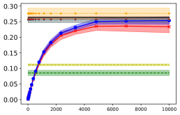
(a) E2S Model

(b) E2ST Model

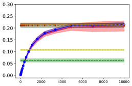
(c) ET Model

Figure 2: Hamming distance between generated samples and the initial synthetic network for a networks on ${n=}50$ vertices; average and standard deviation of $m=$50 trials. In E2S, $2a^{\ast}(1-a^{\ast})=0.263$; in E2ST, $2a^{\ast}(1-a^{\ast})=0.248$; in ET, $2a^{\ast}(1-a^{\ast})=0.217$.

From Figure 2, we see that the parameter estimation methods have largest Hamming distance from the input network. As these methods use the input network only for parameter estimation and then generate networks at random, this finding is perhaps not surprising. However, SteinGen samples have much higher Hamming distance compared to those from CELL, indicating higher sample diversity. With the number of steps in SteinGen,the Hamming distance for both SteinGen_nr and SteinGen samples increases and then stabilises and approaches the theoretical limit ${2}a^{*}(1-a^{*})$ from Proposition 7; this stabilisation provides another natural criterion for the number of steps for which to run SteinGen and SteinGen_nr. While in Section 4.3 the theoretical underpinning gives $N\log N+\gamma N+0.5=9419$ as guideline for the number of steps, in Figure 2 the results are already close to stable for step sizes of around $r=4000$, less than half of $N\log N+\gamma N+0.5$. The variance of the Hamming distance for SteinGen after stabilisation is higher than that of SteinGen_nr, indicating that the re-estimation procedure increases sample diversity. The sample diversity achieved by SteinGen and SteinGen_nr is close to that achieved by the parameter estimation methods.

Fidelity-diversity trade-off

Figure 3 shows the trade-off between fidelity and diversity in the simulated networks. The dotted red line shows the estimated $1-{TV}$ Distance using $50$ simulated networks under the null model. As expected, as the number of steps $r$ increases, the Hamming distances (diversity) for SteinGen samples increases while $1-TV$ Distance (fidelity) decreases. However, the sample fidelity decreases only a by small amount and approaches the empirical total variation distance (the red dashed line). Compared to CELL and NetGAN, SteinGen with large $r$ produces samples with simultaneously higher diversity and higher fidelity. The bound $(\sqrt{n\pi})^{-1}$ from (20) is not too far off.

More synthetic experiments can be found in Appendix B, including different re-estimation intervals for updating the estimates of $\hat{q}$ (Section B.1), examples with multiple graph observations (Section B.2), and improving the sample quality by selecting samples with the smallest gKSS value (Section B.3). The choice of graph kernels in gKSS is explored in detail in Weckbecker et al. (2022).

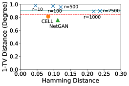
(a) E2S Model

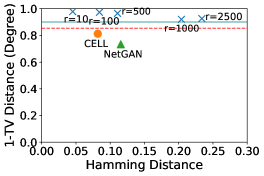
(b) E2ST Model

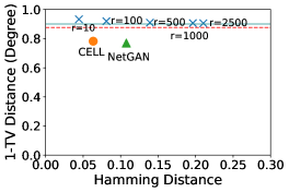
(c) ET Model

Figure 3: Hamming distance versus TV distance of degree using generated samples; $r$ is the number of steps in SteinGen. The estimated error is estimated from simulations, the error bound is the bound $(\sqrt{\pi n})^{-1}$ from (20).

Runtime comparison

The time, in seconds, for generating a sample from each method for our E2ST model, are, in order of speed: SteinGen_nr (0.0244), CELL (0.0487), NetGAN (0.5265), SteinGen (0.0559), MPLE (0.0929), and MLE (0.5090). SteinGen_nr is the fastest method, but it has a less accurate gKSS test rejection rate than SteinGen.

5.3 Real network applications

As a real network example we use a teenager friendship network with 50 vertices described in Steglich et al. (2006); Xu and Reinert (2021) propose an E2ST ERGM. Table 2 shows some of its network summary statistics.

We generate $50$ samples from the input graph and compute the sufficient statistics Edge Density, Number of 2Stars and Number of Triangles for the generated samples from each method; their averages and standard deviations are shown in Table 2. The reported SteinGen values use $r=600$ steps.

Table 2: Teenager friendship network. Closest to observed is in red, second-closest in blue.

	Density	2Stars	Triangles	AgraSSt	Hamming
MPLE	0.0421 (2.42e-2)	329 (80.4)	75.52 (43.4)	0.68	0.106 (2.22e-2)
CD	0.2900 (1.10e-2)	4537 (538)	4146 (668)	0.92	0.211 (1.03e-2)
CELL	0.0450 (3.46e-4)	220 (14.1)	22.50 (7.73)	0.12	0.0423 (3.32e-3)
NetGAN	0.1120 (1.38e-6)	227 (13.3)	9.28 (2.53)	0.34	0.0820 (5.07e-3)
SteinGen_nr	0.0516 (1.02e-3)	362 (14.9)	88.90 (24.8)	0.06	0.0912 (9.95e-3)
SteinGen	0.0445 (9.49e-4)	364 (84.1)	85.75 (10.7)	0.08	0.107 (1.32e-2)
Teenager	0.0458	368	86.00	pval=0.64

For this network, the MCMCMLE estimation procedure in ergm does not converge. CELL captures the edge density and 2-Star statistics well, but not the triangle counts. CD has the highest variability but does not capture the sufficient network statistics. MPLE estimates the sufficient statistics reasonably well but is outperformed by SteinGen. SteinGen_nr also performs well in capturing the sufficient statistics. As the true model for the teenager network is unknown and hence the gKSS test does not apply, in Table 2 we also report the proportion of rejections of the kernel-based Approximate graph Stein Statistic (AgraSSt) goodness-of-fit test (15) to assess the sample quality; see Section 2.4 for details. This test uses an approximate model which estimates the conditional probabilities in Equation 13, given the number of edges, 2stars, and triangles, from the observed Teenager network, without an explicit underlying ERGM.

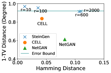
Figure 4: Hamming distance versus $1-TV$ Distance of degree for the teenager network; $r$ is the number of steps in SteinGen, the blue line is the error bound $(n\pi)^{-\frac{1}{2}}$ from (20).

We generate $100$ samples from each method and perform the AgraSSt test using $200$ samples generated from the approximate model to determine the rejection threshold at test level $\alpha=0.05$. We also report the AgraSSt test $p$-value of the Teenager network; the value indicates that the observed network can plausibly be viewed as having the estimated conditional distribution.

Table 2 shows that SteinGen has the rejection rate which is closest to the test level 0.05, followed by SteinGen_nr and CELL, while the parameter estimation methods MPLE and CD have a much higher rejection rate. Regarding diversity, the Hamming distance from CELL is the lowest, indicating that perhaps the generated samples are very similar to the original Teenager network. CD produces the largest Hamming distances on average, but the sample quality is low. The next highest diversity is produced by SteinGen.

Moreover, Table 3 shows some additional standard network statistics to match those used in Rendsburg et al. (2020), except the power law exponent which is not often informative for small networks: shortest path (SP), largest connected components (LCC), assortativity (Assortat.), clustering coefficient (Clust.) and Maximum degree of the network. SteinGen performs the best on first four of these statistics, within one standard deviation of the observed values, closely followed by SteinGen_nr, while the other methods show statistically significant deviation from the observed statistics. However for the maximum degree, NetGAN performs best, although closely followed by SteinGen.

Moreover, we plot the Hamming distance versus $1-TV$ Distance to visualise the trade-off between the quality of generated samples and the diversity. Figure 4 shows that with increasing number of SteinGen steps, the increase in total variation distance is small compared to the gain in Hamming distance. SteinGen produces samples with higher fidelity and, for $r=600$ or $r=2000$, also with larger diversity than CELL and NetGAN.

As an aside, for a network of size $n$ the crude upper bound on the total variation distance of $(n\pi)^{-\frac{1}{2}}$ derived in (20) gives 0.9202115; SteinGen samples are not far off. The effect of different kernel choices for the teenager network is explored in Section C.1, Table 5. While there are numerical differences, the AgraSSt rejection rates are qualitatively similar for the different kernels.

Table 3: Additional network statistics.

	SP	LCC	Assortat.	Clust.	Max(deg)
Teenager	3.39	33.00	0.172	0.9056	5.00
SteinGen	3.49 (0.299)	33.20 (0.678)	0.163 (0.031)	1.027 (0.018)	11.50 (1.688)
SteinGen_nr	3.76 (0.464)	35.25 (2.66)	0.144 (0.056)	1.226 (0.098)	13.00 (1.712)
CELL	5.38 (0.905)	45.30 (5.56)	0.103 (0.089)	0.191 (0.025)	11.20 (0.980)
NetGAN	2.66 (0.034)	33.00 (0.)	0.098 (0.085)	0.132 (0.035)	9.333 (1.014)
MPLE	2.048 (1.17)	20.05 (8.48)	0.765 (0.143)	0.187 (0.024)	11.30 (1.269)
CD	1.148 (0.224)	25.00 (0.100)	0.985 (0.020)	0.190 (0.027)	12.00 (1.673)

6 Conclusion and discussions

SteinGen is a synthetic network generation method which is based on Stein’s method and can be used even when only one input network is available; no training samples are required. In our experiments SteinGen achieves a good balance between a high sample quality as well as a good sample diversity. In Appendix C of the Appendix we include additional experiments on real network experiments, namely the Florentine marriage network from Padgett and Ansell (1993), and two protein interaction networks, for EBV (Hara et al., 2022) and for yeast (Von Mering et al., 2002). In these experiments the general pattern is confirmed, but with sometimes different orderings of CELL and NetGAN. With only one observed network, we find that SteinGen generates synthetic samples which are close in distribution to the observed network while being dissimilar from it. Moreover, SteinGen comes with theoretical guarantees.

SteinGen outperforms its competitors partly through its re-estimation step which implicitly captures variability in the distribution from which the observed network is generated. We also propose a faster method, SteinGen_nr, which avoids the re-estimation step and also performs well. As an intermediary method, one could re-estimate ${\color[rgb]{0,0,0}\widehat{q}(s,1|{\Delta_{s}t(x)})}$ in Algorithm 2 only after a fixed number of samples have been generated, see Section B.1 for details and additional experimental results.

While here SteinGen is presented in the setting of ERGMs, using the AgraSSt  approach from Xu and Reinert (2022b), it is straightforward to generalise the approach to networks for which the underlying distribution family is unknown. Moreover, SteinGen can easily be expanded to take multiple graphs as input, gaining strength in conditional probability estimation; for details see Section B.2 in the Appendix. One could also generate multiple samples and use AgraSSt to select the best samples for the next network generation step, see Section B.3 in the Appendix; this could be viewed as related to particle filtering. Moreover, learning suitable network statistics $t(x)$ could be an interesting future research direction.

SteinGen has some shortcomings: It disregards any attributes on the network. It does not naturally apply to time series of networks. It also does not come with any privacy preserving guarantees. Extending SteinGen to these settings will be part of future work.

Finally a note of caution: when applying SteinGen, ethical aspects should be taken into consideration. One could think of situations in which synthetic networks distort the sensitive narrative of the data. Moreover, if the synthetic networks are used for crucial decision making such as in healthcare, extra care is advised.

Acknowledgments and Disclosure of Funding

The authors would like to thank Chris Oates (Newcastle) for a very helpful discussion. G.R. and W.X. acknowledge the support from EPSRC grant EP/T018445/1. G.R is also supported in part by EPSRC grants EP/W037211/1, EP/V056883/1, and EP/R018472/1. WX is also supported by Deutsche Forschungsgemeinschaft (DFG, German Research Foundation) under Germany’s Excellence Strategy – EXC number 2064/1 – Project number 390727645.

Appendix A More on parameter estimation methods

As shown in Section 5, parameter estimation methods based on MPLE, CD and MLE can achieve high sample diversity but in our experiment they usually show low sample fidelity. To better understand this behaviour here we estimate the parameters in the three models E2S, E2ST and ET in the same setup as in Section 5.2, with $n=50$ vertices and the same true parameter values $\beta_{1}=-2,\beta_{2}=\frac{1}{n},\beta_{3}=-\frac{1}{n}$. We note that parameter estimation methods estimate the parameters jointly for maximising the likelihood; for an observed network $x$ the linear combination $\sum_{l=1}^{L}\beta_{l}t_{l}(x)$ is the basis of the estimation. Hence we would not expect to see unique parameter estimates, but we would expect a linear combination of them to stay approximately constant.

Figure 5 shows the results for the estimates of $\beta_{1}$ versus $\beta_{2}$; the true parameter combination is indicated by a magenta star. In the E2S model, which is arguably the easiest of the three models considered, in all three methods there is an approximately linear relationship between the estimates of $\beta_{1}$ and $\beta_{2}$, relating to maintaining a similar density of the generated graphs. However, in the E2ST and ET models, the parameter estimation can be very inaccurate, for all three methods. Hence, a higher rejection rate in a gKSS test for the parameter estimation methods, as observed in Table 1 in the main text, is not unexpected.

(a) E2S Model

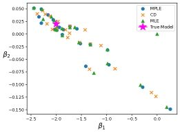
(b) E2ST Model

(c) ET Model

Figure 5: Estimated parameters $\beta_{1}$, $\beta_{2}$ for $n=50$. The plot shows considerable variability in the parameter estimation.

Appendix B More synthetic experiments

In this section, we provide additional experimental results on synthetic networks. When we refer to specific ${\mathrm{ERGM}}$s we use the same parameters as in Section 5.2 in the main text.

B.1 Re-estimation after $k$ steps

In the main text, we present SteinGen with re-estimation after one step in the Glauber dynamics chain; we re-estimate the transition probability when the sampled network differs from the previous network. By construction, the two networks will deviate in one edge indicator, rendering the re-estimation procedure to be not very computationally efficient. Hence it may be of interest to re-estimate the transition probability only after $k$ different networks have been obtained. Here we investigate the setting where the re-estimation happens after $k$ changes in the network (where networks could be repeated, but not consecutively), for networks on 30 vertices. We also consider the setting of SteinGen_nr where no re-estimate applies; one could view this case as $k=\infty$.

(a) E2S Model

(b) E2ST Model

(c) ET Mode

Figure 6: Hamming distance $\pm 1$ standard deviation between generated samples and an initial network from each model for different re-estimation steps, including SteinGen_nr as a benchmark. The number of vertices is set to $30$. For each re-estimation step size $k$ we record the first observations after $k\times n/2$ steps to unify the comparison by accounting for the number of steps in the Glauber process.

(a) E2S Model

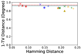
(b) E2ST Model

(c) ET Model

Figure 7: Hamming distance versus 1-TV distance of degree with generated samples; $r$ is the number of steps in SteinGen; $k$ is the number of steps between re-estimation; $n=30$; Est Error is estimated from simulations; Error Bound is $({n\pi})^{-\frac{1}{2}}$ in (20).

We plot the Hamming distance for various models, varying the number of re-estimation steps, in Figure 6. From the plot we see that, with higher number of re-estimation steps $k$, the Hamming distance converges to the limit faster, which is expected and echoes the behavior of SteinGen_nr. Moreover, as $k$ increases, the variance of Hamming distance increases as well, implying an increase in sample variety. Figure 7 shows the relationship between diversity and fidelity; the number of steps in SteinGen has a more substantial effect on diversity than the number of steps between re-estimation. As expected, re-estimation after every step achieves highest fidelity; there is a trade-off between fidelity and computational efficiency.

B.2 Graph generation from multiple network observations

Table 4: Rejection rate for the the gKSS test with $5$ observed network samples; network size $n=30$; test level $\alpha=0.05$. The closest value to the test level is marked in red and the second closest in blue.

Model	E2S	ET	E2ST	ER
MPLE	0.09	0.07	0.08	0.06
CD	0.13	0.17	0.19	0.09
MLE	0.06	0.11	0.07	0.07
SteinGen_nr	0.03	0.06	0.05	0.06
SteinGen	0.04	0.05	0.06	0.04

As mentioned in Section 6, SteinGen can easily be expanded to multiple graph inputs. Heuristically, the estimation of the conditional distribution should be improved when multiple input graphs are available, as it can then be estimated from the collection of graphs. Here we show some experiments to illustrate this extension; we use the same setup as in Section 5.2, on 30 vertices, but now with 5 observed network samples from each model. For the parameter estimation counterparts, we use the ergm.multi implementation recently added to the statnet suite (Krivitsky et al., 2022). To estimate the conditional distribution in Algorithm 1, if there are $c$ observed network samples $x_{1},\ldots,x_{c}$ from each model, on $n$ vertices each, we denote by $N_{i}$ the set of pairs of vertices in network $i$, for $i=1,\ldots,c$, so that $|N_{i}|=N$ for all $i$. Then we estimate

$$q(x^{(s,{1})}|{\Delta_{s}t(x)}=\underline{k})=\frac{\sum_{i=1}^{c}\sum_{s\in N_{i}}\mathbb{I}(x_{i}^{s}=1)\mathbb{I}({\Delta_{s}t(x)}=\underline{k})}{\sum_{i=1}^{c}\sum_{s\in N_{i}}\mathbb{I}({\Delta_{s}t(x)}=\underline{k})}$$

where $\mathbb{I}(A)$ is the indicator function of an event $A$ which equals 1 if $A$ holds and 0 otherwise.
Similarly to what was was carried out for Table 1, a gKSS test is performed; the rejection rates are reported in Table 4. Compared to Table 1, the rejection rates show a marked improvement for all methods; for SteinGen and SteinGen_nr they are now very close to the desired 0.05 even for E2ST. Except on the simple ER network for which SteinGen_nr ties with MPLE, SteinGen and SteinGen_nr again outperform the other methods.

B.3 Improving sample quality with gKSS selection

The standard SteinGen procedure may produce a sampled network which may not be very representative of the true network, judged by gKSS. As mentioned in Section 6, gKSS could also be used as a criterion to select samples for potential downstream tasks. As an illustration, we generate 30 network samples on 30 vertices from the E2S model in Section 5.2, calculate the gKSS for each of these 30 samples, and select the 10 samples with the smallest gKSS value. We repeat this experiment $50$ times. Figure 8 shows a slight improvement in fidelity, but there can be a slight deterioration in diversity, according to our measures.

(a) E2S Model

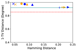
(b) E2ST Model

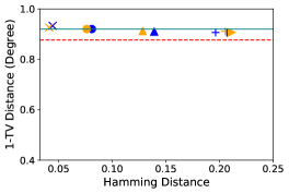
(c) ET Model

Figure 8: Hamming distance versus 1-TV distance of degree using generated samples with and without batch selection; $r$ is the number of steps in SteinGen; Est Error, in red, is estimated from simulations, while Error Bound, in blue, is the bound $(\sqrt{\pi n})^{-1}$ from (20).

Appendix C Additional real data experiments

Here we report results from experiments on additional real network data. In the absence of a ground truth model, we consider a method as performing well if the observed network statistic in the real network is within two standard deviations of the average in the generated samples. In addition we judge diversity by the Hamming distance to the observed real network; the larger the Hamming distance, the more diverse the samples.

C.1 Additional results for the teenager network: kernel choice

In this subsection present further experimental results on the teenager friendship network (Steglich et al., 2006) discussed in Section 5.3.

Table 5: AgraSSt rejection rate at 5% level with different graph kernel choices for the teenager network

	MPLE	CD	CELL	SteinGen	SteinGen_nr
WL	0.68	0.92	0.12	0.06	0.08
GVEH	0.46	0.74	0.36	0.08	0.04
SP	0.34	0.62	0.10	0.02	0.04
Const	0.24	0.32	0.10	0.04	0.06

We investigate the quality of generated samples from various schemes with AgraSSt using different graph kernels. WL: Weisfeiler-Lehman (WL) graph kernels (Shervashidze et al., 2011) with level parameter $3$ as presented in the main text; GVEH Gaussian Vertex-Edge Histogram kernel (Sugiyama and Borgwardt, 2015) with unit bandwidth; SP: the Short Path kernel (Borgwardt and Kriegel, 2005); and Const: the “constant” kernel as considered in Weckbecker et al. (2022). From the rejection rate in Table 5, we see that SteinGen and SteinGen_nr achieve rejection rates which are much closer to the significance level $0.05$ compare to MPLE, CD and CELL. The WL kernel and the constant kernel yield rejection rates which match the 5% level most closely for SteinGen, but other kernels perform fairly similarly, confirming the findings in Weckbecker et al. (2022).

Table 6: Statistics for generated samples from Lazega’s lawyer network; $50$ networks are generated from each methods; reporting average(avg) and standard deviation (sd).

	MPLE	CD	MLE	CELL	NetGAN	SteinGen	SteinGen_nr	Lazega
Density(avg)	0.184	0.191	0.180	0.182	0.205	0.182	0.183	0.183
Density(sd)	0.023	0.018	0.017	0.001	0.003	0.025	0.015	-
2Star(avg)	729.0	785.4	693.1	921.3	899.2	722.3	755.0	926
2Star(sd)	173.2	143.8	126.7	23.7	38.6	133.6	82.7	-
Triangles(avg)	46.2	50.9	42.9	105.4	84.2	139.8	124.8	120
Triangles(sd)	16.4	14.8	12.1	8.25	11.59	38.2	27.8	-
SP (avg)	2.09	2.05	2.10	2.22	2.02	2.12	2.09	2.14
SP (sd)	0.148	0.101	0.096	0.042	0.034	0.073	0.048	-
LCC (avg)	35.9	36.0	35.9	35.9	34.0	36.0	36.0	34
LCC(sd)	0.180	0.	0.300	0.359	0.	0.	0.	-
Assortat.(avg)	-0.071	-0.046	-0.079	-0.164	-0.040	-0.139	-0.033	-0.168
Assortat.(sd)	0.098	0.065	0.091	0.058	0.081	0.069	0.058	-
Clust.(avg)	0.1850	0.1911	0.1831	0.3429	0.2885	0.3418	0.4869	0.3887
Clust.(sd)	0.0281	0.0276	0.0271	0.0222	0.0287	0.0981	0.0903	-
Max deg (avg)	11.30	12.00	11.20	15.53	15.67	11.60	12.10	15.00
Max deg (sd)	1.2688	1.4605	0.9451	1.0241	0.9428	1.6248	1.3747	-
AgraSSt(avg)	0.184	0.214	0.132	0.084	0.135	0.095	0.113	0.054
AgraSSt(sd)	0.182	0.067	0.102	0.034	0.158	0.077	0.066	-
Hamming(avg)	0.293	0.296	0.287	0.056	0.145	0.212	0.215	-
Hamming(sd)	0.019	0.017	0.018	0.007	0.008	0.010	0.012	-

C.2 Padgett’s Florentine marriage network

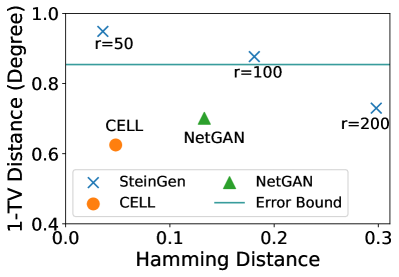
Figure 9: Hamming distance versus 1-TV distance of degree for the Florentine marriage network.

Padgett’s Florentine marriage network (Padgett and Ansell, 1993), with 16 vertices representing Florentine families during the Renaissance and 20 edges representing their marriage ties, is a benchmark network for network analysis. In Reinert and Ross (2019) and Xu and Reinert (2021), an ER model was considered a good fit. Our simulation setup is as in Section 5.3 and we report the same summary statistics in Table 7. The heuristic bound (20) would give a lower bound on the expected value of $0.8589526$ for $1-TV$ Distance.

Figure 9 shows fidelity and diversity for the different methods; here, for large enough $r$, SteinGen achieves considerably higher diversity, and slightly higher fidelity, than CELL or NetGAN.

Table 7: Statistics for generated samples from the Florentine marriage network; reporting average(avg) and standard deviation (sd).

	MPLE	CD	MLE	CELL	NetGAN	SteinGen	SteinGen_nr	Florentine
Hamming	0.268	0.253	0.257	0.048	0.133	0.301	0.268
AgraSSt	0.08	0.10	0.06	0.04	0.06	0.05	0.04	pval=0.15
Density (avg)	0.169	0.160	0.162	0.167	0.190	0.172	0.165	0.167
Density (sd)	0.0361	0.0379	0.0347	2.77e-3	7.75e-4	0.0298	0.0254	-
2Star (avg)	47.66	44.12	44.10	45.86	47.82	63.64	48.80	47
2Star (sd)	20.38	21.39	17.96	3.86	4.59	38.87	15.61	-
Triangles (avg)	2.80	2.72	2.22	2.10	2.42	5.41	4.5	3
Triangles (sd)	2.51	2.36	1.57	1.04	1.47	3.18	2.04	-
SP (avg)	2.543	2.564	2.574	2.704	2.600	2.510	2.439	2.486
SP (sd)	0.339	0.502	0.325	0.188	0.219	0.439	0.254	-
LCC (avg)	14.60	13.86	14.20	15.96	15	15.78	16.00	15
LCC (sd)	1.70	1.91	0.943	0.101	0.	0.229	0.229	-
Assortat. (avg)	-0.141	-0.131	-0.123	-0.328	-0.249	-0.093	-0.132	-0.375
Assortat. (sd)	0.141	0.156	0.158	0.114	0.105	0.107	0.124	-
Clust. (avg)	0.1532	0.1665	0.1474	0.1386	0.2103	0.1532	0.1665	0.1474
Clust. (std)	0.1046	0.1098	0.0841	0.0700	0.0945	0.1046	0.1098	-
Max deg (avg)	4.980	5.060	5.120	6.000	5.167	4.980	5.060	5.120
Max deg (std)	0.1532	0.1665	0.1474	0.1386	1.067	0.1532	0.1665	-

Table 7 gives the result from generating 30 samples each for the different network generators. SteinGen has the largest Hamming distance. While SteinGen samples deviates from some of the observed network statistics more than the other methods, all observed values of the sufficient statistics are well within one standard deviation of the values in the Florentine marriage network. We note that the methods based on parameter estimation perform best for this small benchmark data set.

C.3 Protein-Protein Interaction (PPI) networks

Protein-protein interactions (PPI) are crucial for various biological processes; for a survey see for example Silverman et al. (2020). Here we consider two examples, the Epstein-Barr virus and yeast.

An Epstein-Barr Virus (EBV) network

We first examine a relatively small PPI network, the Epstein-Barr Virus (EBV) network used in (Ali et al., 2014); see also (Hara et al., 2022). This network has one connected component that consists of 60 vertices and 208 edges, thus having edge density 0.11751.

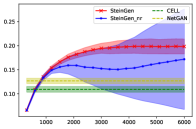
(a) $t=$(E, 2S)

(b) $t$= (E, T)

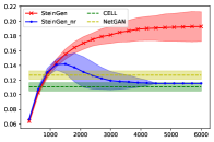
(c) $t$= (E, 2S, T)

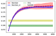
(d) $t$=E

Figure 10: Hamming distance for the Epstein-Barr Virus PPI network

Using different network statistics $t(x)$ we obtain the Hamming distance to the original network in Figure 10. The statistics $t(x)$ used in the models are found in the captions, with $E$ denoting the number of edges, $2S$ the number of 2-stars, and $T$ the number of triangles. We also show the Hamming distance for networks generated by CELL and NetGAN. While SteinGen performs similarly across models, achieving the largest Hamming distance, SteinGen_nr is more erratic in models which include the number of 2-stars. The average and standard deviation are taken over $50$ network samples from each method. The heuristic bound (20) would give a lower bound on the expected value of $0.9271634$ for $1-TV$ Distance.

Table 8 shows various network summaries for generated networks from SteinGen and SteinGen_nr, with $t(x)$ the number of edges and 2-stars, as well as CELL and NetGAN. The network statistics from SteinGen samples are closest or second closest to the observed EBV samples, with a larger standard deviation (std) than CELL or NetGAN samples.The achieved Hamming distances of SteinGen and SteinGen_nr exceed both CELL and NetGAN.

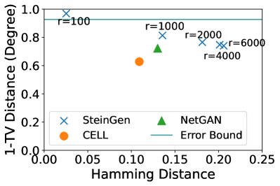
Figure 11: Hamming distance versus 1-TV distance of degree for the EBV network; $r$ is the number of steps in SteinGen.

We show the corresponding fidelity-diversity trade-off plot in Figure 11. The empirical TV distance and Hamming distance are computed from averaging over $50$ samples from each generation method. With $r>1000$, the SteinGen achieves higher fidelity while keeping better diversity compare to CELL and NetGAN. Moreover, the TV distance does not change much from $r=2000$ to $r=6000$.

Table 8: EBV network statistics

	density	2Star	Triangle	Short. Path	LCC	Assortat.	Clust.	Max(deg)
SteinGen	0.1170	1956	214.3	2.318	60.0	-0.1664	0.3524	19.02
std	0.0260	418.7	162.4	0.1447	0.0	0.0586	0.1248	5.863
SteinGen_nr	0.1627	1913	567.5	2.285	59.82	-0.2761	0.5699	25.78
std	0.0281	520.2	206.9	0.1152	0.4331	0.0400	0.1180	3.651
CELL	0.1176	1865	116.0	2.335	60.0	-0.1469	0.1862	21.04
std	1.388e-5	66.78	15.14	0.0323	0.0	0.0581	0.0205	2.441
NetGAN	0.1174	1981	146.5	2.318	60.0	-0.1521	0.2216	22.66
std	1.388e-6	61.38	13.94	0.03699	0.0	0.06409	0.01745	2.405
EBV	0.1175	2277	209.0	2.442	60.0	-0.1930	0.2753	27.0

Table 9: AgraSSt rejection rates for SteinGen on the EBV network with different $t(x)$

	E + 2S	E + T	E + 2S + T	E(Bernoulli)
SteinGen	0.06	0.18	0.12	0.04
SteinGen_nr	0.32	0.58	0.38	0.02
CELL	0.24	0.24	0.22	0.20
NetGAN	0.18	0.20	0.20	0.18

Table 9 gives the rejection rates of AgraSSt tests with different choice of network statistics $t(x)$, based on 50 trials. From the table, we see that the SteinGen samples based on the edges and 2-stars ($E+2S$) and both SteinGen and SteinGen_nr samples based on the Bernoulli model ($E$) tend to be not rejected at $5\%$ significance level. The rejection rate for CELL and NetGAN samples tend to be higher.

A PPI network for yeast

Finally we examine a relatively larger scale standard PPI network, that of yeast based on Von Mering et al. (2002) The network contains 2617 vertices and 11855 edges. We use the largest component (for CELL and NetGAN comparison) as our observed network, which contains 2375 vertices and 11693 edges; giving the edge density of 0.004148. The bound (20) would give a heuristic lower bound on the expected value of $0.9884231$ for $1-TV$ Distance. For both PPI networks, the heuristic bound is much closer to 1, compared to the 1-TV distance of generated samples, indicating that perhaps the independence assumptions in the heuristic are violated.

Figure 12: Hamming distance versus 1-TV distance of degree for the yeast PPI network; $r$ is the number of steps in SteinGen.

Here the theoretical guideline for the choice of $r$, namely $r=N\log N+\gamma N+0.5$, yields $r=43,496,711$. For computational reasons we chose much smaller values of $r$. We report the fidelity-diversity trade-off in Figure 12, where the conditional distribution is estimated using edge and 2-stars. From the plot, we see that the SteinGen method already achieves higher fidelity than the NetGAN, while having larger diversity compared to the CELL and NetGAN samples when the number of steps $r>500$, which is relatively moderate compared to the large graph size of $2375$. When $r$ increases, SteinGen samples achieve higher diversity with minimal sacrifice in sample fidelity.

Table 10: PPI network statistics

	density($10^{-3}$)	2Star($10^{2}$)	Triangle(10)	SP($10^{-3}$)	LCC	Assortat($10^{-4}$).	Clust.($10^{-4}$)	Max(deg)
SteinGen	4.158	3884	6070	5076	2375	4527	4688	118.0
std	6.812e-04	1.241	0.7980	6.149	0.	1.900	1.230	0.
SteinGen_nr	4.159	3885	6072	5067	2375	4521	4689	118.0
std	8.128e-04	2.896	2.517	10.01	0.	5.750	3.890	0.
CELL	4.148	3153	3034	4523	2372	3761	2887	102.5
std	0.	19.63	46.98	25.80	0.8292	101.5	36.60	1.118
NetGAN	3.416	1080	12.23	3821	2617	30.67	33.98	22.67
std	1.479	467.7	5.321	165.4	1133	68.15	14.78	9.849
PPI	4.148	3885	6070	5096	2375	4539	4687	118.0

References

- Abbe and Sandon (2015) Emmanuel Abbe and Colin Sandon. Community detection in general stochastic block models: Fundamental limits and efficient algorithms for recovery. In 2015 IEEE 56th Annual Symposium on Foundations of Computer Science, pages 670–688. IEEE, 2015.
- Ali et al. (2014) Waqar Ali, Tiago Rito, Gesine Reinert, Fengzhu Sun, and Charlotte M Deane. Alignment-free protein interaction network comparison. Bioinformatics, 30(17):i430–i437, 2014.
- Asuncion et al. (2010) Arthur Asuncion, Qiang Liu, Alexander Ihler, and Padhraic Smyth. Learning with blocks: Composite likelihood and contrastive divergence. In Proceedings of the Thirteenth International Conference on Artificial Intelligence and Statistics, pages 33–40. JMLR Workshop and Conference Proceedings, 2010.
- Barbour (1990) Andrew D Barbour. Stein’s method for diffusion approximations. Probability Theory and Related Fields, 84(3):297–322, 1990.
- Besag (1975) Julian Besag. Statistical analysis of non-lattice data. Journal of the Royal Statistical Society: Series D (The Statistician), 24(3):179–195, 1975.
- Bhamidi et al. (2011) Shankar Bhamidi, Guy Bresler, and Allan Sly. Mixing time of exponential random graphs. The Annals of Applied Probability, 21(6):2146–2170, 2011.
- Bojchevski et al. (2018) Aleksandar Bojchevski, Oleksandr Shchur, Daniel Zügner, and Stephan Günnemann. NetGAN: Generating graphs via random walks. In International Conference on Machine Learning, pages 610–619. PMLR, 2018.
- Bollobás et al. (2007) Béla Bollobás, Svante Janson, and Oliver Riordan. The phase transition in inhomogeneous random graphs. Random Structures & Algorithms, 31(1):3–122, 2007.
- Borgwardt and Kriegel (2005) Karsten M Borgwardt and Hans-Peter Kriegel. Shortest-path kernels on graphs. In Fifth IEEE International Conference on Data Mining (ICDM’05), pages 8–pp. IEEE, 2005.
- Bresler et al. (2017) Guy Bresler, David Gamarnik, and Devavrat Shah. Learning graphical models from the Glauber dynamics. IEEE Transactions on Information Theory, 64(6):4072–4080, 2017.
- Butts (2008) Carter T Butts. Social network analysis with sna. Journal of Statistical Software, 24:1–51, 2008.
- Chami et al. (2022) Ines Chami, Sami Abu-El-Haija, Bryan Perozzi, Christopher Ré, and Kevin Murphy. Machine learning on graphs: A model and comprehensive taxonomy. Journal of Machine Learning Research, 23(89):1–64, 2022.
- Chanpuriya et al. (2021) Sudhanshu Chanpuriya, Cameron Musco, Konstantinos Sotiropoulos, and Charalampos Tsourakakis. On the power of edge independent graph models. Advances in Neural Information Processing Systems, 34:24418–24429, 2021.
- Chatterjee and Diaconis (2013) Sourav Chatterjee and Persi Diaconis. Estimating and understanding exponential random graph models. The Annals of Statistics, 41(5):2428–2461, 2013.
- Chwialkowski et al. (2016) Kacper Chwialkowski, Heiko Strathmann, and Arthur Gretton. A kernel test of goodness of fit. In International Conference on Machine Learning, pages 2606–2615. PMLR, 2016.
- Craig (1962) CC Craig. On the mean and variance of the smaller of two drawings from a binomial population. Biometrika, 49(3/4):566–569, 1962.
- Figueira and Vaz (2022) Alvaro Figueira and Bruno Vaz. Survey on synthetic data generation, evaluation methods and GANs. Mathematics, 10(15):2733, 2022.
- Goldstein and Rinott (1996) Larry Goldstein and Yosef Rinott. Multivariate normal approximations by Stein’s method and size bias couplings. Journal of Applied Probability, 33(1):1–17, 1996.
- Gorham and Mackey (2015) Jackson Gorham and Lester Mackey. Measuring sample quality with Stein’s method. In Advances in Neural Information Processing Systems, pages 226–234, 2015.
- Goyal et al. (2020) Nikhil Goyal, Harsh Vardhan Jain, and Sayan Ranu. GraphGen: a scalable approach to domain-agnostic labeled graph generation. In Proceedings of The Web Conference 2020, pages 1253–1263, 2020.
- Guo and Zhao (2022) Xiaojie Guo and Liang Zhao. A systematic survey on deep generative models for graph generation. IEEE Transactions on Pattern Analysis and Machine Intelligence, 2022.
- Han et al. (2022) Yuehui Han, Le Hui, Haobo Jiang, Jianjun Qian, and Jin Xie. Generative subgraph contrast for self-supervised graph representation learning. In Computer Vision–ECCV 2022: 17th European Conference, Tel Aviv, Israel, October 23–27, 2022, Proceedings, Part XXX, pages 91–107. Springer, 2022.
- Handcock et al. (2008) Mark S Handcock, David R Hunter, Carter T Butts, Steven M Goodreau, and Martina Morris. statnet: Software tools for the representation, visualization, analysis and simulation of network data. Journal of Statistical Software, 24(1):1548, 2008.
- Hara et al. (2022) Yuya Hara, Takahiro Watanabe, Masahiro Yoshida, HM Abdullah Al Masud, Hiromichi Kato, Tomohiro Kondo, Reiji Suzuki, Shutaro Kurose, Md Kamal Uddin, Masataka Arata, et al. Comprehensive analyses of intraviral Epstein-Barr virus protein–protein interactions hint central role of BLRF2 in the tegument network. Journal of Virology, 96(14):e00518–22, 2022.
- Hein et al. (2007) Matthias Hein, Jean-Yves Audibert, and Ulrike von Luxburg. Graph laplacians and their convergence on random neighborhood graphs. Journal of Machine Learning Research, 8(6), 2007.
- Hinton (2002) Geoffrey E Hinton. Training products of experts by minimizing contrastive divergence. Neural Computation, 14(8):1771–1800, 2002.
- Hoff et al. (2002) Peter D Hoff, Adrian E Raftery, and Mark S Handcock. Latent space approaches to social network analysis. Journal of the American Statistical association, 97(460):1090–1098, 2002.
- Holland and Leinhardt (1981) Paul W Holland and Samuel Leinhardt. An exponential family of probability distributions for directed graphs. Journal of the American Statistical Association, 76(373):33–50, 1981.
- Hunter and Handcock (2006) David R Hunter and Mark S Handcock. Inference in curved exponential family models for networks. Journal of Computational and Graphical Statistics, 15(3):565–583, 2006.
- Hunter et al. (2008a) David R Hunter, Steven M Goodreau, and Mark S Handcock. Goodness of fit of social network models. Journal of the American Statistical Association, 103(481):248–258, 2008a.
- Hunter et al. (2008b) David R Hunter, Mark S Handcock, Carter T Butts, Steven M Goodreau, and Martina Morris. ergm: A package to fit, simulate and diagnose exponential-family models for networks. Journal of Statistical Software, 24(3):nihpa54860, 2008b.
- Jiang et al. (2018) Bai Jiang, Tung-Yu Wu, Yifan Jin, and Wing H Wong. Convergence of contrastive divergence algorithm in exponential family. The Annals of Statistics, 46(6A):3067–3098, 2018.
- Karwa et al. (2016) Vishesh Karwa, Sonja Petrović, and Denis Bajić. DERGMs: Degeneracy-restricted exponential random graph models. arXiv preprint arXiv:1612.03054, 2016.
- Kingma and Ba (2014) Diederik P Kingma and Jimmy Ba. Adam: A method for stochastic optimization. arXiv preprint arXiv:1412.6980, 2014.
- Kolaczyk (2009) Eric D Kolaczyk. Statistical analysis of network data. Springer Series in Statistics, 2009.
- Krivitsky et al. (2022) Pavel N Krivitsky, Martina Morris, Mark S Handcock, Carter T Butts, David R Hunter, Steven M Goodreau, Chad Klumb, Skye Bender de Moll, and Michał Bojanowski. Advanced features of the ergm package for modeling networks. network, 1:2, 2022.
- Krivitsky et al. (2023) Pavel N. Krivitsky, David R. Hunter, Martina Morris, and Chad Klumb. ergm 4: New features for analyzing exponential-family random graph models. Journal of Statistical Software, 105(6):1–44, 2023. doi: 10.18637/jss.v105.i06.
- Liu et al. (2016) Qiang Liu, Jason Lee, and Michael Jordan. A kernelized Stein discrepancy for goodness-of-fit tests. In International Conference on Machine Learning, pages 276–284, 2016.
- Liu et al. (2017) Weiyi Liu, Pin-Yu Chen, Hal Cooper, Min Hwan Oh, Sailung Yeung, and Toyotaro Suzumura. Can GAN learn topological features of a graph? arXiv preprint arXiv:1707.06197, 2017.
- Lovász and Szegedy (2006) László Lovász and Balázs Szegedy. Limits of dense graph sequences. Journal of Combinatorial Theory, Series B, 96(6):933–957, 2006.
- Mukherjee and Xu (2023) Sumit Mukherjee and Yuanzhe Xu. Statistics of the two star ERGM. Bernoulli, 29(1):24–51, 2023.
- Newman (2018) Mark Newman. Networks. Oxford University Press, 2. edition, 2018.
- Niu et al. (2020) Chenhao Niu, Yang Song, Jiaming Song, Shengjia Zhao, Aditya Grover, and Stefano Ermon. Permutation invariant graph generation via score-based generative modeling. In International Conference on Artificial Intelligence and Statistics, pages 4474–4484. PMLR, 2020.
- Padgett and Ansell (1993) John F Padgett and Christopher K Ansell. Robust Action and the Rise of the Medici, 1400-1434. American Journal of Sociology, 98(6):1259–1319, 1993.
- Reinert and Ross (2019) Gesine Reinert and Nathan Ross. Approximating stationary distributions of fast mixing Glauber dynamics, with applications to exponential random graphs. The Annals of Applied Probability, 29(5):3201–3229, 2019.
- Rendsburg et al. (2020) Luca Rendsburg, Holger Heidrich, and Ulrike Von Luxburg. NetGAN without GAN: From random walks to low-rank approximations. In Proceedings of the 37th International Conference on Machine Learning, pages 8073–8082. PMLR, 2020.
- Schmid and Desmarais (2017) Christian S Schmid and Bruce A Desmarais. Exponential random graph models with big networks: Maximum pseudolikelihood estimation and the parametric bootstrap. In 2017 IEEE International Conference on Big Data, pages 116–121. IEEE, 2017.
- Shalizi and Rinaldo (2013) Cosma Rohilla Shalizi and Alessandro Rinaldo. Consistency under sampling of exponential random graph models. Annals of Statistics, 41(2):508, 2013.
- Shervashidze et al. (2011) Nino Shervashidze, Pascal Schweitzer, Erik Jan van Leeuwen, Kurt Mehlhorn, and Karsten M Borgwardt. Weisfeiler-Lehman graph kernels. Journal of Machine Learning Research, 12(Sep):2539–2561, 2011.
- Silverman et al. (2020) Edwin K Silverman, Harald HHW Schmidt, Eleni Anastasiadou, Lucia Altucci, Marco Angelini, Lina Badimon, Jean-Luc Balligand, Giuditta Benincasa, Giovambattista Capasso, Federica Conte, et al. Molecular networks in network medicine: Development and applications. Wiley Interdisciplinary Reviews: Systems Biology and Medicine, 12(6):e1489, 2020.
- Simonovsky and Komodakis (2018) Martin Simonovsky and Nikos Komodakis. GraphVAE: Towards generation of small graphs using variational autoencoders. In Artificial Neural Networks and Machine Learning–ICANN 2018: 27th International Conference on Artificial Neural Networks, Rhodes, Greece, October 4-7, 2018, Proceedings, Part I 27, pages 412–422. Springer, 2018.
- Snijders (2002) Tom AB Snijders. Markov chain Monte Carlo estimation of exponential random graph models. Journal of Social Structure, 3(2):1–40, 2002.
- Soon (1996) Spario YT Soon. Binomial approximation for dependent indicators. Statistica Sinica, pages 703–714, 1996.
- Sosa and Buitrago (2021) Juan Sosa and Lina Buitrago. A review of latent space models for social networks. Revista Colombiana de Estadística, 44(1):171–200, 2021.
- Steglich et al. (2006) Christian Steglich, Tom AB Snijders, and Patrick West. Applying SIENA. Methodology, 2(1):48–56, 2006.
- Strauss and Ikeda (1990) David Strauss and Michael Ikeda. Pseudolikelihood estimation for social networks. Journal of the American Statistical Association, 85(409):204–212, 1990.
- Sugiyama and Borgwardt (2015) Mahito Sugiyama and Karsten Borgwardt. Halting in random walk kernels. In Advances in Neural Information Processing Systems, pages 1639–1647, 2015.
- Vignac et al. (2022) Clement Vignac, Igor Krawczuk, Antoine Siraudin, Bohan Wang, Volkan Cevher, and Pascal Frossard. Digress: Discrete denoising diffusion for graph generation. arXiv preprint arXiv:2209.14734, 2022.
- Von Mering et al. (2002) Christian Von Mering, Roland Krause, Berend Snel, Michael Cornell, Stephen G Oliver, Stanley Fields, and Peer Bork. Comparative assessment of large-scale data sets of protein–protein interactions. Nature, 417(6887):399–403, 2002.
- Wasserman and Faust (1994) Stanley Wasserman and Katherine Faust. Social Network Analysis: Methods and Applications, volume 8. Cambridge University Press, 1994.
- Weckbecker et al. (2022) Moritz Weckbecker, Wenkai Xu, and Gesine Reinert. On RKHS choices for assessing graph generators via kernel Stein statistics. arXiv preprint arXiv:2210.05746, 2022.
- Xu and Reinert (2021) Wenkai Xu and Gesine Reinert. A Stein goodness-of-test for exponential random graph models. In International Conference on Artificial Intelligence and Statistics, pages 415–423. PMLR, 2021.
- Xu and Reinert (2022a) Wenkai Xu and Gesine Reinert. AgraSSt: Approximate graph Stein statistics for interpretable assessment of implicit graph generators; version 4. arXiv preprint arXiv:2203.03673, 2022a.
- Xu and Reinert (2022b) Wenkai Xu and Gesine D Reinert. AgraSSt: Approximate graph Stein statistics for interpretable assessment of implicit graph generators. Advances in Neural Information Processing Systems, 35:24268–24279, 2022b.
- Yang et al. (2018) Jiasen Yang, Qiang Liu, Vinayak Rao, and Jennifer Neville. Goodness-of-fit testing for discrete distributions via Stein discrepancy. In International Conference on Machine Learning, pages 5557–5566, 2018.
- Yin et al. (2016) Mei Yin, Alessandro Rinaldo, and Sukhada Fadnavis. Asymptotic quantization of exponential random graphs. The Annals of Applied Probability, pages 3251–3285, 2016.
- You et al. (2018) Jiaxuan You, Rex Ying, Xiang Ren, William Hamilton, and Jure Leskovec. GraphRNN: Generating realistic graphs with deep auto-regressive models. In International Conference on Machine Learning, pages 5708–5717. PMLR, 2018.