PT-symmetric dynamical confinement:
Fermi acceleration, quantum force and Berry phase
Abstract
We consider a quantum particle under the dynamical confinement caused by PT-symmetric box with a moving wall. The latter is described in terms of the time-dependent Schrödinger equation obeying the time-dependent PT-symmetric boundary conditions. The class of the functions, describing time-dependence of the wall’s position and keeping the system as PT-symmetric is found. Physically observable characteristics, such as average kinetic energy and the average quantum force are calculated as a function of time. Also, geometric phase is calculated for the harmonically oscillating wall regime. Experimental realization of the proposed model is discussed.
I Introduction
Since the publication of the pioneering paper by Bender and Boettcher Bender98 , parity-time symmetric quantum systems attracted much attention Bender07 - [8] . It was long believed that only Hermitian Schrödinger operators can describe physical systems. However, Bender with Boettcher refuted such a statement. They argued that also some non-Hermitian but PT-symmetric operators could have real eigenvalues and play, therefore, the role of acceptable quantum Hamiltonians.
This conjecture caused rapidly growing interest in PT-symmetric quantum physics. Different aspects of the topic have been studied both in quantum mechanical and field theoretical contexts. A huge number of papers dealing with various issues of PT-symmetric quantum physics have been published during the past two decades. These studies allowed one to construct various mathematically consistent theories of PT-symmetric quantum systems including even several innovative non-Hermitian but PT-symmetric quantum field theories Bender99 -Ours19_02 .
Experimental realization of such systems was also the subject of extensive research. The latter has been done mainly in optics [6] ; Ganainy07 ; Ruter10 . Some other PT-symmetric systems have been discussed recently in the literature Znojil09 ; Znojil17_03 ; Znojil17_04 ; Znojil22_01 . General theory of PT-symmetric quantum mechanics have been developed introducing so-called PT-symmetric inner product. However, since such a condition does not provide a positively definite norm, its extension in terms of a PCT-symmetric inner product was proposed in Bender02_02 ; Mostafazadeh02 ; Bender07 ; Bender08_02 ; Znojil08 .
Within such a theory a PT-symmetric model can be introduced either through the complex potential, or by imposing proper boundary conditions, which provide such symmetry via the inner product. Different types of complex potentials that provide PT-symmetry in the Hamiltonian have been considered in Bender07 , Bender08_02 . Introducing PT-symmetry in terms of proper boundary conditions was studied for the particle-in-box systems in Bender18_01 or Znojil91 ; Znojil05 ; Znojil06 ; Znojil12 .
In this paper we propose a model for dynamical confinement in a PT-symmetric well by considering hard-wall box with moving boundaries. The system is assumed to satisfy PT-symmetric hard-wall boundary conditions. The corresponding quantum dynamics is described in terms of time-dependent Schrödinger equation upon which time-dependent boundary conditions are imposed. In other words, we will solve the Schrödinger equation endowed with PT-symmetric, time-dependent boundary conditions.
II Hermitian model
We note that the conventional Hermitian Schrödinger equation with time-dependent boundary conditions have been the topic for extensive research during past four decades, especially, for 1D case (see, e.g., Refs.doescher -Uzy22 ). Early treatments of the dynamical confinement in nonrelativistic quantum mechanics date back to Doescher, who studied basic aspects of the problem doescher . Munier et al. studied more detailed research of the problem and calculated physically observable quantities for the problem of time-dependent box mun81 . Later, Makowsky mak91 -mak923 and Razavy razavy01 ; razavy02 provided a systematic study of the dynamical confinement problem, by considering one-dimensional box with moving walls and classifying time-dependence of the wall approving exact solution of the Schrödinger equation with time-varying boundary conditions. Unitary transformation that maps the time-dependent box to that with fixed walls, was found in razavy01 ; razavy02 . These studies used an approach developed earlier by Berry and Klein berry00 . Different aspects of the problem dynamical confinement and its applications to dynamical Casimir effect was studied in a series of papers by Dodonov et al. dodonov01 -dodonov04 . Berry phase in time-dependent box was studied in per ; Kwon ; Wang . Šeba studied the problem of time-dependent box in the context of quantum Fermi acceleration seb90 . The quantum gas under the dynamical confinement was considered in nakamura01 ; nakamura02 , where quantum force operator for time-dependent box was introduced. Hydrogen-like atom confined in a spherical hard-wall box with time-varying radius was considered in Our03 . Different aspects of the problem of dynamical confinement were studied also in pinder -glas09 . The problem of time-dependent Neumann boundary conditions is considered in duca . Extension of the dynamical confinement to relativistic case by considering Dirac equation for time-dependent box was done in sobirov . Time-dependent quantum graphs have been considered in the Refs. matrasulov ; nikiforov ; Uzy22 .
Let us now briefly recall Hermitian counterpart of our model the one-dimensional problem of studying the quantum dynamics of a particle confined in box with time-varying wall, following the Ref. mak91 . The dynamics of the particle in such system can be described by the time-dependent Schrödinger equation ()
| (1) |
with time dependent Dirichlet boundary conditions
| (2) |
Here, is the wave function of the quantum particle. Introducing a new coordinate, allows us to get the wave equation imposed static boundary conditions as
| (3) |
with new boundary conditions given by
| (4) |
III Static PT-symmetric quantum box
Time-independent counterpart of our system, i.e. the PT-symmetric particle-in-box system has been considered earlier in the Refs. Znojil06 ; Znojil12 ; Dasarathy13 ; Znojil15 . Here we will briefly recall its description following the Ref. Znojil12 . For one-dimensional Schrödinger equation given as
| (7) |
PT-symmetry of the system is provided by Robin type boundary condition which is given as Znojil12
| (8) |
and .
The solution of Eq. (7) fulfilling the PT-symmetric boundary condition given by Eq. (8) can be written as
| (9) |
here the is the normalization constant given by
Corresponding eigenvalues can be written as
| (10) |
where is the quantum number.
IV PT-symmetric quantum box with a moving wall
A time-dependent version of the above PT-symmetric boundary condition given by Eq. (8) can be written as
| (11) |
for some and for all , where the time evolution is given in terms of the Schrödinger equation (1). Following the approach from Section III, one has here a kind of -symmetry. Namely let be the parity and the time reversal operators, which are defined as
| (12) |
If
| (13) |
denotes the Hamilton operator.
Here -symmetry means that whenever is a wave function satisfying the above -symmetric boundary condition (11), then one has
| (14) |
and the function also satisfies the -symmetric boundary condition (11).
We show that this is satisfied for the Hamiltonian in (13) and -symmetric boundary condition (11). Indeed, using the definition of and , it is easy to see
which shows (14). Moreover, if a wave function satisfies the boundary condition (11), then
One can see from equation above, this system is -symmetric, if is an even function, i.e. ,
| (15) |
We note that norm conservation is broken for the boundary conditions (11):
which is non-zero, hence the norm is not conserved.
Solving the Eq. (1) with the Robin-type boundary conditions (11) is difficult because of the time-dependent boundary conditions. In order to change the time-dependent boundary conditions into static ones we use two transformations. One of them is for the coordinate and is given by
| (16) |
Substituting the transformation in (16) into the equation gives
| (17) |
with
| (18) |
for all and .
Using the second transformation for the wave function
| (19) |
We get
| (20) |
with static Neumann boundary conditions as
| (21) |
for all .
Eq. (20) can be solved by expanding the wave function in terms of the static box eigenfunctions fulfilling the Neumann boundary conditions
| (22) |
By substituting (22) into Eq. (20), we obtain
| (23) |
Multiplying both sides of this equation to , integrating over and using the orthonormal property, , we obtain asystem of first order differential equations for the expansion coefficients ,
| (24) |
where
| (25) |
with
| (26) |
and
| (27) |
V Quantum dynamics under PT-symmetric time-dependent confinement
Quantum dynamics of a particle under PT-symmetric confinement can be studied by analyzing time-dependence of such characteristics as the average kinetic energy, average quantum force and (for adiabatically evolving system), so-called geometric phase, or Berry phase. Average kinetic energy describes acceleration or deceleration of the particle under the dynamical confinement. In case of harmonically oscillating wall, it serves as the main characteristic of so-called Fermi acceleration. The average quantum force describes the expectation value of the force acting by moving wall of the box to a particle confined inside the box. Geometric phase appears in a quantum system, where the evolution is caused by a slowly varying parameter.
V.1 The average kinetic energy
The average kinetic energy is determined as the expectation value of the kinetic energy operator:
| (28) |
where is as in (13).
For PT-symmetric quantum box with a moving wall, using Eqs. (22) and (24), the average kinetic energy can be written as
| (29) |
It is clear that is a real function of time, despite the complex boundary conditions in Eq. (11). Also, it is easy to see that for the expression for coincides with that for its Hermitian counterpart (see, e.g. Refs. doescher ; nakamura01 ).
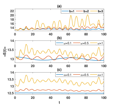
The average kinetic energy as a function of time is presented in Fig. 1 for (a) different values of the amplitude, (b) frequency and c PT-symmetric para meter, . For all cases, fluctuates in time and there is no monotonic growth or decay of the average kinetic energy as a function of time. This is a specific property of PT-symmetric systems: Pumping of energy does not cause monotonic growth, as the system undergoes to losses.
V.2 The average force
During its motion the wall of the box interacts with confined particle. This interaction appears in the form of pressure by the wall to the particle. Such pressure is caused by the quantum force which is described in terms of the force operator as
| (30) |
The expectation value of the force operator can be written as nakamura01
| (31) |
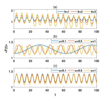
In Fig. 2 plots of are presented as a function of time for harmonically oscillating wall at different values of the oscillation amplitude (a), oscillation frequency (b) and parameter (c). Unlike the behavior of the time-dependence of demonstrates certain quasi-periodicity in (a) and (b). Even periodic time-dependence can we observed in the plots of in Fig. 2c.
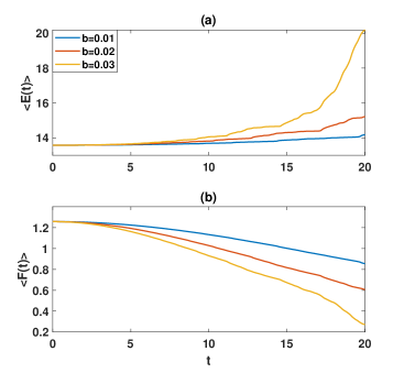
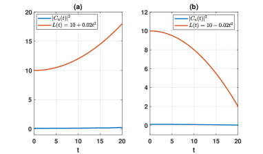
An important case for the above model is monotonically expanding or contracting which is directly related, e.g. to the problem of the behaviour of matter under the very heavy pressure and cooling of quantum ideal gas. Fig. 3 presents the plots of the average kinetic energy (a) and force (b) as a function of time for quadratically (in time) expanding box at different values of acceleration of the wall . Unlike the case of the Hermitian counterpart, where contracting of the box’s size causes growth of the average kinetic energy, Fig. 3a demonstrates decrease of . This happens due to the second term in Eq. (29), which contains the factor , growing much faster than .
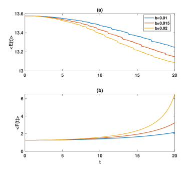
Completely opposite behaviour can be seen in time-dependence of presented in Fig. 3b. Here the average force decays in time like in case of Hermitian counterpart of our system. This can be explained by the fact that second term in Eq. (31) dos not depend on , while first contains the factor , which growth much faster than that of the second term. This can be clearly seen from Fig. 5a which compares and . In Fig. 4 the average kinetic energy (a) and force (b) are plotted as a function of time for quadratically contracting box at different values of acceleration of the wall . In this case average energy decays as a function of time, while decays. This also can be explained from Fig. 5b, where and are compared as a function of time.
V.3 Geometric phase
The case of slowly evolving system in the context of dynamical confinement is of importance. If such evolution occurs due to a slowly varying parameter of the system it can be considered as an adiabatic evolution. An interesting feature of such a system is the existence of so-called geometric phase found by Berry in the Ref. Berry84 . Berry showed that for a quantum system evolving adiabatically due to a slowly varying parameter, if the parameter adiabatic changes along the closed curve, in the parameter space, the wave function of the system can acquire the so-called geometrical phase in addition to the dynamical one. This additional phase (called later ”Berry phase”) is different from zero when the trajectory of the system in the parameter space is located near a point at which the states of the system are degenerate. Berry phase for Hermitian counterpart of our model was studied earlier in the Refs. dodonov02 ; Kwon ; Wang . For PT-symmetric systems Berry phase becomes complex Hayward18 -Fring23 . In our case, when time-varying parameters is the position of the wall of the box, this corresponds very slowly moving wall, i.e. slowly varying position of the wall, . For slowly moving wall in our model, the Berry phase can be written as Berry84
| (32) |

Solution of the Eq. (32) imposed PT-symmetric Robin type boundary conditions (11) can be written as
| (33) |
with eigenvalues and normalization coefficient .
The geometric phase can be directly computed using its definition given in Berry84 :
| (34) |
where is the period of the function .
In case of the harmonically oscillating wall , substituting (33) into Eq. (34) gives us
| (35) |
Indeed, is complex for our system. Although Berry phase is computed for a special case of a harmonically oscillating wall, one can do such calculation for different regimes of the wall’s motion, provided for this regime keeps PT-symmetry of the system.
V.4 A sketch for experimental realization
Here we discuss ways for experimental realization of our model. Despite the great progress made in theoretical study of different aspects of PT-symmetric quantum physics, experimental realization of such systems in quantum mechanical processes has not yet been achieved. The only possible way for experimental study of PT-symmetry is using optical systems, who can ”mimic” due to the fact that propagation of light in such media can be described in terms of Helmholtz equation formally coinciding with the Schrödinger equation. The sketch we propose here also is based on the use of optical media. Most easiest and direct way could be a sketch presented in Fig. 6. It consist of absorbing (loss) and active (gain) materials containing empty space (the void) between them. The motion of the electromagnetic wave, ( ) within the void is described in terms of Eq. (7), with the PT-symmetric boundary condition, given by Eq. (8). Moving boundaries can be provided by mechanical way, i.e. by shifting the positions of absorbing and active media. Another option for experimental realization of our model can be using so-called PT-symmetric waveguides Borisov08 ; Turitsyna17 , providing Robin boundary conditions at the edges. Mechanical motion of the waveguide can produce time-dependent counterpart of such conditions. Finally, the third option could be dynamical version of the so-called electromagnetic analog of the PT-symmetric box, considered in the Ref. Dasarathy13 , where one could consider travelling waves insted of standing ones.
VI Conclusions
In this work we studied dynamical confinement in a -symmetric quantum system created by a quantum box with a moving wall. The system is described in terms of the Schrödinger equation with time-varying boundary conditions. The exact solution of the problem is obtained for different regimes of the wall’s motion. Such physically observable characteristics as average kinetic energy, average quantum force and average coordinate are computed as a function of time. Geometric phase is analytically calculated for an harmonically oscillating wall. Experimental realization of the model is discussed by proposing a sketch based on the use of PT-symmetric gain and loss media, as well as PT-symmetric waveguides. The model proposed in this paper can be used for the study of different aspects of dynamical confinement in pseudo-Hermitian systems, including Berry phase in different regimes of the wall’s motion. The limits of adiabatically moving and sudden removal of the wall, as well as the case of atom confined in PT-symmetric box are the subjects for forthcoming studies.
References
- (1) C.M. Bender, S. Boettcher, Phys. Rev. Lett. 80 5243 (1998).
- (2) C.M. Bender, Rep. Prog. Phys. 70 94 (2007).
- (3) A. Mostafazadeh, Int. J. Geom. Methods Mod. Phys. 7 1191 (2010).
- (4) F. Bagarello, J.-P. Gazeau, F. Szafraniec, M. Znojil (Eds.), Non-Selfadjoint Operators in Quantum Physics: Mathematical Aspects, Wiley, Hoboken (2015).
- (5) D. Christodoulides, J.-K. Yang (Eds.), Parity-Time Symmetry and Its Applications, Springer Verlag, Singapore (2018).
- (6) C.M. Bender (Ed.), PT Symmetry in Quantum and Classical Physics, World Sci entific, Singapore (2018).
- (7) M. Znojil, in: Ref. [5] , pp. 7–58
- (8) C.M. Bender, S. Boettcher, P.N. Meisinger, J. Math. Phys. 40 2201 (1999).
- (9) C.M. Bender, S. Boettcher, V.M. Savage, J. Math. Phys. 41 6381 (2000).
- (10) C.M. Bender, Q. Wang, J. Phys. A: Math. Gen. 34 3325 (2001).
- (11) C.M. Bender, D.C. Brody, H.F. Jones, Phys. Rev. Lett. 89 270401 (2002).
- (12) C.M. Bender, S. Boettcher, P.N. Meisinger, Q. Wang, Phys. Lett. A 302 286 (2002).
- (13) A. Mostafazadeh, J. Math. Phys. 43 205 (2002).
- (14) C.M. Bender, D.C. Brody, H.F. Jones, Am. J. Phys. 71 1095 (2003).
- (15) C.M. Bender, D.C. Brody, H.F. Jones, Phys. Rev. Lett. 93 251601 (2004).
- (16) C.M. Bender, J.H. Chen, K.A. Milton, J. Phys. A: Math. Gen. 39 1657 (2006).
- (17) C.M. Bender, D.W. Hook, J. Phys. A: Math. Theor. 41 392005 (2008).
- (18) C.M. Bender, P.D. Mannheim, Phys. Rev. D 78 025022 (2008).
- (19) M. Znojil, SIGMA 4 001 (2008).
- (20) M. Znojil, Phys. Rev. D 80 045022 (2009).
- (21) C.M. Bender, P.D. Mannheim, Phys. Lett. A 374 1616 (2010).
- (22) S. Schindler, C.M. Bender, J. Phys. A: Math. Theor. 51 055201 (2018).
- (23) C.M. Bender, C. Ford, N. Hassanpour, B. Xia, J. Phys. Commun. 2 025012 (2018).
- (24) A. Mostafazadeh, J. Phys. A: Math. Gen. 36 7081 (2003).
- (25) A. Szameit, M.C. Rechtsman, O. Bahat-Treidel, M. Segev, Phys. Rev. A 84 021806 (2011).
- (26) O. Yesiltas, J. Phys. A: Math. Theor. 46 015302 (2013).
- (27) Y.X. Zhao, Y. Lu, Phys. Rev. Lett. 118 056401 (2017).
- (28) M. Znojil, Phys. Lett. A 285 7 (2001).
- (29) M. Znojil, J. Math. Phys. 46 062109 (2005).
- (30) D. Krejčiřík, H. Bíla, M. Znojil, J. Phys. A: Math. Gen. 39 10143 (2006).
- (31) M. Znojil, Can. J. Phys. 90 1287 (2012).
- (32) A. Dasarathy, J. P. Isaacson, K. Jones-Smith, J. Tabachnik, H. Mathur, Phys. Rev. A, 154 062111 (2013).
- (33) M. Znojil, Can. J. Phys. 93 765 (2015).
- (34) M. Znojil, F. Ruzicka, K. G. Zloshchastiev, Symmetry 9 165 (2017).
- (35) M. Znojil, Phys. Rev. A 96 012127 (2017).
- (36) M. Znojil, I. Semoradova, F. Ruzicka, H. Moulla, I. Leghrib, Phys. Rev. A 95 042122 (2017).
- (37) M. Znojil, Ann. Phys. (NY) 385 162 (2017).
- (38) D.U. Matrasulov, K.K. Sabirov, J.R. Yusupov, J. Phys. A: Math. Theor. 52 155302 (2019).
- (39) M. Znojil, Math. 10 3721 (2022).
- (40) M. Znojil, EPL 139 32001 (2022).
- (41) M. Znojil, Eur. Phys. J. Plus 137 335 (2022).
- (42) M. Znojil, Phys. Lett. A 421 127792 (2022).
- (43) R. El-Ganainy, K.G. Makris, D.N. Christodoulides, Z.H. Musslimani, Opt. Lett. 32 2632 (2007).
- (44) Ch.E. Rüter et al, Nat. Phys. 6 192 (2010).
- (45) M. Chitsazi, H. Li, F.H. Ellis, T. Kottos, Phys. Rev. Lett. 119 093901 (2017).
- (46) S. Longhi, Phys. Rev. A 95 012125 (2017).
- (47) J. Yusupov, S. Rakhmanov, D. Matrasulov, H. Susanto, J. Phys. A: Math. Theor. 52 055303 (2019).
- (48) S.W. Doescher, H.H. Rice, Am. J. Phys. 37 1246 (1969).
- (49) P. Pereshogin, P. Pronin, Phys. Lett. A 156 12 (1991).
- (50) A. Munier, J.R. Burgan, M. Feix, E. Fijalkow, J. Math. Phys. 22 1219 (1981).
- (51) M. Razavy, Lett. Nuovo Cimento 37 13, 30 Luglio (1983).
- (52) M.V. Berry, G. Klein, J. Phys. A 17 1805 (1984).
- (53) A.J. Makowski, S.T. Dembinski, Phys. Lett. A 154 217 (1991).
- (54) A.J. Makowski, P. Peptowski, Phys. Lett. A 163 142 (1992).
- (55) A.J. Makowski, J. Phys. A: Math. Gen. 25 3419(1992).
- (56) M. Razavy, Phys. Rev. A 44 2384 (1991).
- (57) V.V. Dodonov, V.I. Man’ko, D.E. Nikonov, Phys. Lett. A 162 359 (1992).
- (58) V.V. Dodonov, A.B. Klimov, D.E. Nikonov, J. Math. Phys. 34, 2742 (1993).
- (59) J. Dittrich, P. Duclos, J. Phys. A: Math. Gen. 35 8213 (2002).
- (60) V.V. Dodonov, A.V. Dodonov, J. Phys. A: Math. Gen.39 6271 (2006).
- (61) A.V. Dodonov, B. Militello, A. Napoli, A. Messina, Phys. Rev. A 93 052505 (2016).
- (62) P. Pereshogin, P. Pronin, Phys. Lett. A 156 12 (1991).
- (63) O. Kwon, Y. Kim, Ch. Lee, J. Phys. A . 25 6113 (1992).
- (64) A-L. Wang, F-P. Liu, Mod. Phys. Lett. B, 28 1450122 (2014).
- (65) P. Šeba. Phys. Rev. A 41 2306 (1990).
- (66) K. Nakamura, S.K. Avazbaev, Z.A. Sobirov, D.U. Matrasulov, T. Monnai, Phys. Rev. E 83, 041133, (2011).
- (67) K. Nakamura, Z.A. Sobirov, D.U. Matrasulov, S.K. Avazbaev, Phys. Rev. E 86 061128 (2012).
- (68) S. Rakhmanov, D. Matrasulov, V.I. Matveev, Eur, J. Phys. D 72 177 (2018).
- (69) D.N. Pinder, Am. J. Phys. 58 54 (1990).
- (70) C. Scheiniger, M.Kleber, Physica D 50 391 (1991).
- (71) J.D. Lejarreta, J. Phys. A 32 4749 (1999).
- (72) L. Ling, L. Bo-Zang, Phys. Lett. A 291 190 (2001).
- (73) C. Yuce, Phys. Lett. A 321 291 (2004).
- (74) T.K. Jana, P. Roy, Phys. Lett. A. 372 2368 (2008).
- (75) M.L. Glasser, J. Mateo, J. Negro, L.M. Nieto, Chaos, Solitons and Fractals 41 2067 (2009).
- (76) A. Duca, R. Joly, Ann. Henri Poincare 22 2029 (2021).
- (77) Z.A. Sobirov, D. Matrasulov, Sh. Ataev, H. Yusupov, , in: G. Casati, D. Matrasulov(eds.): Complex Phenomena in Nanoscale Systems, (Springer, Dordrecht), p. 215 (2009).
- (78) D.U. Matrasulov, J.R. Yusupov, K.K. Sabirov, Z.A. Sobirov, Nanosystems: Phys. Chem. Math. 6 173, (2015).
- (79) D.S. Nikiforov, I.V. Blinova, I.Y. Popov, Indian J. Phys. 93 913 (2019).
- (80) U. Smilansky, G. Sofer, ArXiv:2210.14652v1 (2022).
- (81) M.V. Berry, Proc. R. Soc. Lond. A 392 45 (1984).
- (82) R. Hayward, F. Biancalana, Phys. Rev. A 98 053833 (2018).
- (83) J. Gong, Q. Wang, Phys. Rev. A 82 012103 (2010).
- (84) S. Longhi, L. Feng, Phys. Rev. B 107 085122 (2023).
- (85) A. Fring, T. Taira, R. Tenney, J. Phys. A: Math. Theor. 56 12LT01 (2023).
- (86) D. Borisov and D. Krejčiřík, Integr. equ. oper. theory 62 489 (2008).
- (87) E. G. Turitsyna, I. V. Shadrivov, Y. S. Kivshar, Phys. Rev. A 96 033824 (2017).