Differentially Private Dual Gradient Tracking
for Distributed Resource Allocation

Abstract

This paper investigates privacy issues in distributed resource allocation over directed networks, where each agent holds a private cost function and optimizes its decision subject to a global coupling constraint through local interaction with other agents. Conventional methods for resource allocation over directed networks require all agents to transmit their original data to neighbors, which poses the risk of disclosing sensitive and private information. To address this issue, we propose an algorithm called differentially private dual gradient tracking (DP-DGT) for distributed resource allocation, which obfuscates the exchanged messages using independent Laplacian noise. Our algorithm ensures that the agents’ decisions converge to a neighborhood of the optimal solution almost surely. Furthermore, without the assumption of bounded gradients, we prove that the cumulative differential privacy loss under the proposed algorithm is finite even when the number of iterations goes to infinity. To the best of our knowledge, we are the first to simultaneously achieve these two goals in distributed resource allocation problems over directed networks. Finally, numerical simulations on economic dispatch problems within the IEEE 14-bus system illustrate the effectiveness of our proposed algorithm.

, , , ,

1 Introduction

Resource allocation (RA) problems have been crucial in various fields like smart grids [1] and wireless sensor networks [2], involving collaborative optimization of agents’ objective functions while satisfying global and local constraints. Centralized approaches face drawbacks like single point failures, high communication demands, and substantial computational costs [3, 4], prompting the rise of distributed frameworks reliant on interactions among neighboring agents.

The primary challenge in distributed resource allocation (DRA) is managing global resource constraints that couple all agents’ decisions. Zhang and Chow [5] devised a leader-follower consensus algorithm for quadratic objectives. To relax the assumption on the quadratic form of cost functions, Yi et al. [6] developed a primal-dual algorithm. These studies focused on undirected networks with doubly stochastic information mixing matrix, but bidirectional information flows may waste communication costs and not be present due to the heterogeneous communication power of sensors. To address this, Yang et al. [1] proposed a distributed algorithm for unbalanced directed networks using the gradient push-sum method, but involved an additional procedure for agents to asymptotically calculate the eigenvector of the weight matrix. In a subsequent study, Zhang et al. [7] leveraged the dual relationship between DRA and distributed optimization (DO) problems, exploring the push-pull technique for explicit convergence rate determination.

However, the above literature assumes secure transmission of raw information, but the distributed nature of cyber-physical systems raises privacy concerns. Messages exchanged between agents are vulnerable to interception by attackers, risking the theft or inference of sensitive data. For instance, in economic dispatch problems over smart grids, transmitted messages may reveal private user patterns or financial status, posing security threats. Therefore, it is vital to develop privacy-preserving algorithms for distributed resource allocation. While encryption is a classical method to prevent eavesdropping [8], it may not be feasible for large-scale distributed agents with limited battery capacity. Differential privacy (DP) has gained attention for its rigorous mathematical formulation and privacy assurance in statistical databases [9].

For unconstrained DO problems, some studies have recently developed differentially private algorithms over directed networks. Chen et al. [10] incorporated state-decomposition and constant noise for privacy-preserving DO. However, it only preserves privacy per iterations and thus the cumulative privacy loss increases to infinity over time. Additionally, their convergence and privacy analysis relied on the boundedness of the gradient, which is impractical in many applications such as the distributed economic dispatch with commonly used quadratic cost functions. Wang et al. [11] relaxed the bounded gradient assumption and ensured the $\varepsilon$-DP over infinite iterations, but they require that the adjacency gradients should be the same near the optimal point. Huang et al. [12] have shown that the gradient tracking-based algorithm cannot reach $\epsilon$-DP when the stepsizes chosen are not summable under Laplacian noise. These works all assume that the cost functions are strongly convex or convex and ignore potential global constraints. For DRA with global coupling constraints, Han et al. [13] achieved DP for constraints by adding noise to public signals, but this requires an extra entity for information collection and broadcasting. Ding et al. [14] and Wu et al. [15] preserved the privacy of cost functions for distributed resource allocation, but these works are limited to undirected networks. To the best of our knowledge, there is no work deal with differentially private DRA over directed networks.

Motivation by the aforementioned observations, our work focuses on providing DP for DRA over directed graphs. We focus on the privacy guarantee for $\delta$-adjacent distributed resource allocation problems (Definition 2.2), which relaxes the assumption of bounded gradients. To deal with the global coupling constraints, we focus on the dual counterpart of DRA. However, despite the dual relationship between DO and DRA as well as the mentioned advanced private DO algorithms over directed works, it is noteworthy that the dual objective function related to distributed resource allocation is not always strongly convex. Therefore, the analysis methods in [10, 12] cannot be used in our work. Therefore, we analyze the convergence of gradient-tracking with noisy shared information, even for non-convex objectives, which significantly extends the analysis in previous studies [10, 11, 12]. We derive conditions for the step size and noise to ensure convergence and $\epsilon$-DP over infinite iterations simultaneously. We present in Table 1 a comparison of some the most relevant works.

Table 1: A Comparison of Some Related Decentralized Algorithms.

	Problem	Network Graph	Gradient Assumption	DP Consideration
[7]	DRA	Directed	No assumption	$\times$
[14, 15]	DRA	Undirected	Adjacent gradients should be the same in the horizontal position	$\epsilon$-DP over infinite iterations
[10]	DO (strongly convex)	Directed	The gradient is uniformly bounded	The gradient is uniformly bounded
[11]	DO (convex)	Directed	The adjacent gradients are the same near the optimal point	$\epsilon$-DP over infinite iterations
[12]	DO (strongly convex)	Directed	The distance between adjacent gradients is bounded	$\epsilon$-DP over infinite iterations
Our work	DRA	Directed	The distance between adjacent gradients is bounded	$\epsilon$-DP over infinite iterations

In summary, our main contributions are as follows:

• We propose a differentially private dual gradient tracking algorithm, abbreviated as DP-DGT (Algorithm 1), to address privacy issues in DRA over directed networks. Our algorithm masks the transmitted messages in networks with Laplacian noise and does not rely on any extra central authority.

• With the derived sufficient conditions, we prove that the DP-DGT algorithm converges to a neighborhood of the optimal solution (Theorem 4.11) by showing the convergence of the dual variable even for non-convex objectives (Theorem 4.9). This theoretical analysis nontrivially extends existing works on gradient tracking with information-sharing noise for convex or strongly convex objectives [10, 11, 12].

• We specify the mathematical expression of privacy loss $\epsilon$ under the DP-DGT (Theorem 5.12) and demonstrate that the DP-DGT algorithm preserves DP for each individual agent’s cost function even over infinite iterations (Corollary 5.14). To our best knowledge, previous studies have only reported differential privacy results for DRA in undirected networks [14, 15]. Moreover, our analysis relaxes the gradient assumption used in [11, 10].

The remainder of this paper is organized as follows. Preliminaries and the problem formulation of privacy-preserving DRA over directed networks are provided in Section 2. A differentially private distributed dual gradient tracking algorithm with robust push-pull is proposed in Section 3. Then, details on the convergence analysis are presented in Section 4, followed by a rigorous proof of $\epsilon$-DP over infinite iterations in Section 5. Numerical simulations are presented to illustrate the obtained results in Section 6. Finally, conclusions and future research directions are discussed in Section 7.

Notations: Let $\mathbb{R}^{p}$ and $\mathbb{R}^{p\times q}$ represent the set of $p$-dimensional vectors and $p\times q$-dimensional matrices, respectively. The notation $\mathbf{1}_{p}\in\mathbb{R}^{p}$ denotes a vector with all elements equal to one, and $I_{p}\in\mathbb{R}^{p\times p}$ represents a $p\times p$-dimensional identity matrix. We use $\|\cdot\|_{2}$ or $\|\cdot\|$ to denote the $\ell_{2}$-norm of vectors and the induced $2$-norm for matrices. We use $\mathbb{P}(\mathcal{A})$ to represent the probability of an event $\mathcal{A}$, and $\mathbb{E}[x]$ to be the expected value of a random variable $x$. The notation $\text{Lap}(\theta)$ denotes the Laplace distribution with probability density function $f_{L}(x|\theta)=\frac{1}{2\theta}e^{\frac{-|x|}{\theta}}$, where $\theta>0$. If $x\sim\text{Lap}(\theta)$, we have $\mathbb{E}[x^{2}]=2\theta^{2}$ and $\mathbb{E}[x]=0$.

Graph Theory: A directed graph is denoted as $\mathcal{G}=(\mathcal{N},\mathcal{E})$, where $\mathcal{N}=\{1,2,\dots,N\}$ is the set of nodes and $\mathcal{E}\subseteq\mathcal{N}\times\mathcal{N}$ is the edge set consisting of ordered pairs of nodes. Given a nonnegative matrix $\mathbf{A}=[a_{ij}]\in\mathbb{R}^{N\times N}$, the directed graph induced by $\mathbf{A}$ is referred to as $\mathcal{G}_{\mathbf{A}}=(\mathcal{N},\mathcal{E}_{\mathbf{A}})$, where the directed edge $(i,j)$ from node $j$ to node $i$ exists, i.e., $(i,j)\in\mathcal{E}_{\mathbf{A}}$ if and only if $a_{ij}>0$. For a node $i\in\mathcal{N}$, its in-neighbor set $\mathcal{N}_{\mathbf{A},i}^{\text{in}}$ is defined as the collection of all individual nodes from which $i$ can actively and reliably pull data in graph $\mathcal{G}_{\mathbf{A}}$. Similarly, its out-neighbor set $\mathcal{N}_{\mathbf{A},i}^{\text{out}}$ is defined as the collection of all individual agents that can passively and reliably receive data from node $i$.

2 Preliminaries and Problem Statement

In this section, we will provide some preliminaries and problem formulations. First, we introduce the problem of RA over networks, along with its dual counterpart in network settings. Next, we discuss the class of algorithms we will be considering and provide an overview of the messages that are communicated. We then highlight the potential privacy concerns in traditional algorithms and introduce concepts related to DP. Finally, we formulate the problems that will be addressed in this work.

2.1 Resource Allocations over Networks

We consider a network of $N$ agents that interact on a directed graph $\mathcal{G}$ to collaboratively address a RA problem. Each agent $i$ possesses a local private cost function $F_{i}:\mathbb{R}^{m}\to\mathbb{R}$. Their goal is to solve the following resource allocation problem using a distributed algorithm over $\mathcal{G}$:

$$\min_{\mathbf{w}\in\mathbb{R}^{N\times m}} \quad F(\mathbf{w})=\sum_{i=1}^{N}F_{i}(w_{i}),$$ (1)

$$s.t. \quad\sum_{i=1}^{N}w_{i}=\sum_{i=1}^{N}d_{i},\ w_{i}\in\mathcal{W}_{i},\ \forall i\in\mathcal{N},$$

where $w_{i}\in\mathbb{R}^{m}$ represents the local decision of agent $i$, indicating the resource allocated to the agent, $\mathcal{W}_{i}\subseteq\mathbb{R}^{m}$ refers to the local closed and convex constraint set, $\mathbf{w}=[w_{1},\dots,w_{N}]^{T}\in\mathbb{R}^{N\times m}$, and $d_{i}$ denotes the local private resource demand of agent $i$. Let $d=\sum_{i=1}^{N}d_{i}$, and thus $\sum_{i=1}^{N}w_{i}=d$ represents the overall balance between supply and demand, indicating the coupling among agents.

Throughout the paper, we make the following assumptions:

Assumption 1.

(Strong convexity and Slater’s condition):

• The local cost function $F_{i}$ is $\mu$-strongly convex for all $i\in\mathcal{N}$, i.e., for any $w,w^{\prime}\in\mathbb{R}^{m}$, $\|\nabla F_{i}(w)-\nabla F_{i}(w^{\prime})\|\geq\mu\|w-w^{\prime}\|$.

• There exists at least one point in the relative interior $\mathcal{W}$ that can satisfy the power balance constraint $\sum_{i=1}^{N}w_{i}=\sum_{i=1}^{N}d_{i}$, where $\mathcal{W}=\mathcal{W}_{1}\times\cdots\times\mathcal{W}_{N}$.

Assumption 1 ensures strong duality between problem (1) and its dual counterpart, enabling us to deal with the coupling constraint based on its dual problem.

2.2 Dual Problem

Let us introduce the class of DRA algorithms we are considering in this paper. To handle the global constraint, we begin by formulating the dual problem of (1). The Lagrange function of (1) is given by

$$\mathcal{L}(\mathbf{w},x)=\sum_{i=1}^{N}F_{i}(w_{i})+x^{T}\left(\sum_{i=1}^{N}w_{i}-\sum_{i=1}^{N}d_{i}\right),$$ (2)

where $x\in\mathbb{R}^{m}$ represents the dual variable. Thus, the dual problem of (1) can be expressed by

$$\max_{x\in\mathbb{R}^{m}}\ \inf_{\mathbf{w}\in\mathcal{W}}\mathcal{L}(\mathbf{w},x).$$ (3)

The objective function in (3) can be written as

$$\inf_{\mathbf{w}\in\mathcal{W}}\mathcal{L}(\mathbf{w},x)$$

$$= \inf_{\mathbf{w}\in\mathcal{W}}\left\{\sum_{i=1}^{N}F_{i}(w_{i})+x^{T}\left(\sum_{i=1}^{N}w_{i}-\sum_{i=1}^{N}d_{i}\right)\right\}$$

$$= \sum_{i=1}^{N}\inf_{w_{i}\in\mathcal{W}_{i}}\left(F_{i}(w_{i})+x^{T}w_{i}\right)-x^{T}\sum_{i=1}^{N}d_{i}$$

$$= \sum_{i=1}^{N}-F_{i}^{*}(-x)-x^{T}\sum_{i=1}^{N}d_{i},$$

where

$$F_{i}^{*}(x)=\sup_{w_{i}\in\mathcal{W}_{i}}\left(x^{T}w_{i}-F_{i}(w_{i})\right)$$ (4)

corresponds to the convex conjugate function for the pair $(F_{i},\mathcal{W}_{i})$ [16]. Consequently, the dual problem (3) can be formulated as the subsequent DO problem

$$\min_{\mathbf{x}\in\mathbb{R}^{m}}\ f(x)=\sum_{i=1}^{N}f_{i}(x),\ \text{where}\ f_{i}(x)\triangleq F_{i}^{*}(-x)+x^{T}d_{i}.$$ (5)

According to the Fenchel duality between strong convexity and the Lipschitz continuous gradient [17, 18], the strong convexity of $F_{i}$ indicates the differentiability of $F_{i}^{*}$ with Lipschitz continuous gradients, and the supremum in (4) can be attained. Danskin’s theorem states that $\nabla F_{i}^{*}(x)=\mathop{\arg\max}\limits_{w\in\mathcal{W}_{i}}\{x^{T}w-F_{i}(w)\}$ [16], providing the gradient of $F_{i}^{*}$. Therefore, we have

$$\nabla f_{i}(x) =-\nabla F_{i}^{*}(-x)+d_{i}$$ (6)

$$=-\mathop{\arg\min}\limits_{w\in\mathcal{W}_{i}}\left\{F_{i}(w)+x^{T}w\right\}+d_{i}.$$

We find that the dual gradient $\nabla f_{i}(x)$ captures the local deviation or mismatch between resource supply and demand, i.e., $w_{i}-d_{i}$, in some sense.

If Assumption 1 holds, we observe the strong duality between the dual DO problem (3) and the primal DRA problem (1). This equivalence is captured through $F^{*}=-f^{*}$ and the optimal solution $x^{*}$ of (3) satisfies $F_{i}^{*}(w_{i}^{*})+F_{i}^{*}(-x^{*})=-x^{*T}w_{i}^{*}$. As a result, if the proposed algorithm can drive the dual variable in (5) to the optimal one, it equivalently steers $\mathbf{w}$ to the optimal solution $\mathbf{w}^{*}$ in (1). Hence, our algorithmic focus can be directed towards solving (5), the standard DO problem.

2.3 Communication Networks and Information Flows

Gradient-tracking with push-pull [19] is one of the DO algorithms that enable agents to solve optimization problems in directed networks, particularly for those unbalanced networks lacking doubly stochastic weight matrices. Solving the dual counterpart (5) using this algorithm allows agents to obtain the optimal solution for the DRA problem (1) over $\mathcal{G}$. Specifically, agent $i$ maintains a local estimate of the dual variable $x$ and a local estimate of the global constraint deviation at iteration $k$, denoted as $\tilde{w}_{i,k}$ and $z_{i,k}$, respectively. These two local variables are shared using two different communication networks, $\mathcal{G}_{\mathbf{R}}$ and $\mathcal{G}_{\mathbf{C}^{T}}$, respectively. These two networks are induced by matrices $\mathbf{R}=[R_{ij}]\in\mathbb{R}^{N\times N}$ and $\mathbf{C}=[C_{ij}]\in\mathbb{R}^{N\times N}$, respectively, where $R_{ij}>0$ for any $j\in\mathcal{N}_{\mathbf{R},i}^{\text{in}}$ and $C_{ij}>0$ for any $i\in\mathcal{N}_{\mathbf{C},j}^{\text{out}}$. We call this special class of algorithms DRA with dual gradient tracking, denoted as $\mathcal{A}$. A representative form of $\mathcal{A}$ that we consider in this paper is as follows [7]:

$$\tilde{w}_{i,k+1}= \sum_{j=1}^{N}R_{ij}\tilde{w}_{j,k}+\beta_{k}z_{i,k},$$ (7a)

$$w_{i,k+1}= \mathop{\arg\min}\limits_{w\in\mathcal{W}_{i}}\left\{F_{i}(w)-\tilde{w}_{i,k+1}^{T}w\right\},$$ (7b)

$$z_{i,k+1}= \sum_{j=1}^{N}C_{ij}z_{j,k}-\iota(w_{i,k+1}-w_{i,k}),$$ (7c)

where $\beta_{k}>0$ and $\iota>0$ are the step sizes.

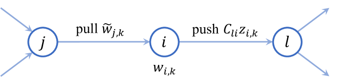
Figure 1: Information flows of agent $i$ under algorithm $\mathcal{A}$.

Fig. 1 illustrates the information flows under algorithm $\mathcal{A}$ over the communication network. At each iteration, agent $i$ pushes $C_{li}z_{i,k}$ to each out-neighboring agent $l\in\mathcal{N}_{\mathbf{C},i}^{\text{out}}$, pulls the dual variable estimate $\tilde{w}_{j,k}$ from its in-neighboring agent $j\in\mathcal{N}_{\mathbf{R},i}^{\text{in}}$, and updates its privately-owned primal optimization variable $w_{i,k}$.

We impose the following assumptions on the communication graphs:

Assumption 2.

The graphs $\mathcal{G}_{\mathbf{R}}$ and $\mathcal{G}_{\mathbf{C}^{T}}$ each contains at least one spanning tree. Moreover, there exists at least one node that is a root of a spanning tree for both $\mathcal{G}_{\mathbf{R}}$ and $\mathcal{G}_{\mathbf{C}^{T}}$.

Assumption 3.

The matrix $\mathbf{R}$ is row-stochastic and $\mathbf{C}$ is column-stochastic, i.e., $\mathbf{R}\mathbf{1}=\mathbf{1}$ and $\mathbf{1}^{T}\mathbf{C}=\mathbf{1}^{T}$.

Assumption 2 is less restrictive than previous works such as [20, 21], as it does not necessitate a strongly connected directed graph. This allows more flexibility in graph design. However, directly transmitting $\tilde{w}_{j,k}$ and $C_{li}z_{i,k}$ in the network will pose privacy concerns, which we will discuss in the next subsection.

2.4 Differential Privacy

In deterministic optimization problems, given a specific initialization and topology, the generated data and decisions are uniquely determined by the cost function of each agent. Therefore, in insecure networks, agents should protect the privacy of their cost functions against eavesdroppers while calculating the optimal solution to (1) in a distributed manner. In this paper, we consider the following commonly used eavesdropping attack model [11, 10]:

Definition 2.1.

An eavesdropping attack is an adversary that is able to listen to all communication messages in the network.

Note that our definition of eavesdropping models a powerful attack as the adversary potentially can intercept every message in the network. For example, in the communication network shown in Fig. 1, an adversary under eavesdropping attack can obtain $\{\tilde{w}_{i,k},C_{li}z_{i,k}|\forall i\in\mathcal{N},k\geq 0\}$. With this observation, the attacker is able to learn $w_{i,k}$ based on publicly known $\mathbf{R}$, $\mathbf{C}$, and step sizes. If the local constraint set $\mathcal{W}_{i}$ is equal to $\mathbb{R}^{m}$ and $F_{i}$ is differentiable, the step (7b) can be rewritten as $w_{i,k+1}=\nabla^{-1}F_{i}(\tilde{w}_{i,k+1})$, where $\nabla^{-1}F_{i}$ represents the inverse function of $\nabla F_{i}$ such that $\nabla F_{i}(w_{i,k+1})=\tilde{w}_{i,k+1}$. As a result, the cost function $F_{i}$ could be deduced from (7b), which causes privacy leakage.

The potential privacy leakage in algorithms in $\mathcal{A}$ motivates us to design novel privacy-preserving algorithms to protect the privacy of agents’ cost functions. To measure privacy, we introduce concepts associated with DP [9].

First, we formulate the closeness of DRA problems. We denote the DRA problem shown in (1) as $\mathcal{P}$ and represent it by four parameters $(\mathcal{W},\mathcal{S},F,\mathcal{G})$, where $\mathcal{S}\subseteq\{\mathbb{R}^{m}\to\mathbb{R}\}$ is a set of real-valued cost functions, and $F=\sum_{i=1}^{N}F_{i}$ with $F_{i}\in\mathcal{S}$ for each $i\in\mathcal{N}$. Specifically, we define $\delta$-adjacency of two DRA problems by measuring the distance between gradients of the individual’s local cost function.

Definition 2.2.

($\delta$-adjacency) Two distributed resource allocation problems $\mathcal{P}$ and $\mathcal{P}^{\prime}$ are $\delta$-adjacent if the following conditions hold:

• they share identical domains for resource allocation and communication graphs, i.e., $\mathcal{W}=\mathcal{W}^{\prime}$ and $\mathcal{G}=\mathcal{G}^{\prime}$;

• there exists an $i_{0}\in\mathcal{N}$ such that $F_{i_{0}}\neq F^{\prime}_{i_{0}}$, and for all $i\neq i_{0}$, $F_{i}=F^{\prime}_{i}$;

• the distance of gradients of $F_{i_{0}}$ and $F^{\prime}_{i_{0}}$ are bounded by $\delta$ on $\mathcal{W}_{i_{0}}$, i.e., $\sup\limits_{w\in\mathcal{W}}\|\nabla F_{i_{0}}(w)-\nabla F_{i_{0}}^{\prime}(w)\|\leq\delta$ for any $w\in\mathcal{W}_{i_{0}}$.

Remark 2.3.

According to Definition 2.2, two DRA problems are considered adjacent when the cost function of a single agent changes, while all other conditions remain the same. It is worth noting that $\delta$-adjacency relaxes requirements from previous works such as [22, 10] by avoiding the need for bounded gradients, making it applicable for quadratic cost functions that are typically utilized in resource allocation problems [1, 23, 24]. Moreover, we do not require the adjacent gradient to be the same as in [11].

Traditional algorithms in $\mathcal{A}$ do not have any privacy protection in general [7]. To preserve the privacy of agents, we should add some random perturbations or uncertainties to confuse the eavesdropper. We denote the class of algorithms $\mathcal{A}$ with random perturbations as $\mathcal{R}$. Given a DRA problem $\mathcal{P}$, an iterative randomized algorithm can be considered as a mapping as $\mathcal{R}_{\mathcal{P}}(v_{0}):v_{0}\to\mathcal{O}$, where $v_{0}$ is the set of initial states of the algorithm $\mathcal{R}$ and $\mathcal{O}$ is the observation sequence of all shared messages.

Let us now define privacy for such a randomized algorithm following the classical $\epsilon$-DP notion introduced by Dwork [9].

Definition 2.4.

($\epsilon$-DP) For a given $\epsilon>0$, a randomized iterative algorithm $\mathcal{R}$ solving (1) is $\epsilon$-DP if for any two $\delta$-adjacent resource allocation problems $\mathcal{P}$ and $\mathcal{P}^{\prime}$, any set of observation sequences $\mathcal{O}\subseteq\emph{Range}(\mathcal{R})$ and any initial state $v_{0}$, it holds that

$$\mathbb{P}[\mathcal{R}_{\mathcal{P}}(v_{0})\in\mathcal{O}]\leq e^{\epsilon}\mathbb{P}[\mathcal{R}_{\mathcal{P}^{\prime}}(v_{0}))\in\mathcal{O}],$$ (8)

where the probability is over the randomness introduced in each iteration of the algorithm.

Definition 2.4 specifies that a randomized algorithm $\mathcal{R}(\cdot)$ preserves $\epsilon$-DP by ensuring small differentiation in output probabilities for two $\delta$-adjacent RA problems. Additionally, $\epsilon$ is commonly referred to as the privacy budget or privacy loss since a small $\epsilon$ indicates the challenge for an eavesdropper to distinguish between two sets of cost functions with high probability based on observed data. However, in many existing works [10, 25, 26], a finite cumulative privacy budget is obtained only over a finite number of iterations. As time goes by, despite nearing optimal points, the privacy will eventually be compromised. Therefore, we meticulously design the step size and noise parameters to preserve privacy.

2.5 Problem Formulation

In this work, we consider first how to design a novel distributed algorithm $\mathcal{R}$ that preserves privacy for RA problems on directed graphs. Then, we focus on the analysis of the conditions for step sizes and perturbations that enable simultaneous achievement of convergence and $\epsilon$-DP over an infinite number of iterations.

3 Algorithm Development

DP is typically preserved by introducing noise into transmitted data. However, when there is information-sharing noise, the exchanged messages become corrupted, and the agents can only receive distorted versions of the estimates of dual variables and constraint deviations, leading to a reduction in accuracy. Thus, a fundamental trade-off exists between the level of privacy and optimization accuracy in differential privacy. To understand the impact of noise, we start by analyzing the update of $\tilde{w}_{i,k}$ and $z_{i,k}$ under the traditional algorithm (7) in the presence of information-sharing noise.

Defining $\tilde{\mathbf{w}}_{k}=[\tilde{w}_{1,k},\dots,\tilde{w}_{N,k}]^{T}\in\mathbb{R}^{N\times m}$ and $\mathbf{z}_{k}=[z_{1,k},\dots,z_{N,k}]^{T}\in\mathbb{R}^{N\times m}$, we can rewrite (7a) and (7c) in their compact forms:

$$\tilde{\mathbf{w}}_{k+1} =\mathbf{R}\tilde{\mathbf{w}}_{k}+\beta_{k}\mathbf{z}_{k},$$ (9a)

$$\mathbf{z}_{k+1} =\mathbf{C}\mathbf{z}_{k}-\iota(\mathbf{w}_{k+1}-\mathbf{w}_{k}).$$ (9b)

By setting $\mathbf{1}^{T}\mathbf{z}_{0}=-\iota\left(\sum_{i=1}^{N}w_{i,0}-\sum_{i=1}^{N}d_{i}\right)$, we can deduce using induction that

$$\mathbf{1}^{T}\mathbf{z}_{k}=-\iota\left(\sum_{i=1}^{N}w_{i,k}-\sum_{i=1}^{N}d_{i}\right),$$

which implies that the agents can track the global mismatch between resource supply and demand.

However, when exchanged messages are subject to noise, i.e., the received values are $\tilde{w}_{i,k}+\zeta_{i,k}$ and $z_{i,k}+\xi_{i,k}$ instead of $\tilde{w}_{i,k}$ and $z_{i,k}$, respectively, the update of the conventional algorithm (9) becomes

$$\tilde{\mathbf{w}}_{k+1} =\mathbf{R}(\tilde{\mathbf{w}}_{k}+\bm{\zeta}_{k})+\beta_{k}\mathbf{z}_{k},$$ (10a)

$$\mathbf{z}_{k+1} =\mathbf{C}(\mathbf{z}_{k}+\bm{\xi}_{k})-\iota(\mathbf{w}_{k+1}-\mathbf{w}_{k}),$$ (10b)

where $\bm{\zeta}_{k}=\left[\zeta_{1,k},\dots,\zeta_{N,k}\right]^{T}\in\mathbb{R}^{N\times m}$, $\bm{\xi}_{k}=\left[\xi_{k},\dots,\xi_{N,k}\right]^{T}\in\mathbb{R}^{N\times m}$, and $\zeta_{i,k}\in\mathbb{R}^{m}$ and $\xi_{i,k}\in\mathbb{R}^{m}$ are injected noises. Using induction, we can deduce that even under $\mathbf{1}^{T}\mathbf{z}_{0}=-\iota\left(\sum_{i=1}^{N}w_{i,0}-\sum_{i=1}^{N}d_{i}\right)$:

$$\mathbf{1}^{T}\mathbf{z}_{k}=-\iota\left(\sum_{i=1}^{N}w_{i,k}-\sum_{i=1}^{N}d_{i}\right)+\sum_{l=0}^{k-1}\mathbf{1}^{T}\bm{\xi}_{l}.$$ (11)

Therefore, under the conventional algorithm, the information-sharing noise accumulates over iterations in the tracking, increasing total variance as iterations proceed. This noise accumulation significantly affects the accuracy of optimization.

To address the limitations of existing dual gradient-tracking-based algorithms [7, 14, 15] and mitigate the impact of information-sharing noise, we draw inspiration from the robust push-pull [27] and let each agent share the cumulative deviation estimate $s_{i,k}$ instead of the direct estimate of per-step global deviation, $z_{i,k}$. Our proposed privacy-preserving method is described in Algorithm 1.

1:Input: Step size sequence $\{\alpha_{k}\}$, noise sequences $\{\xi_{i,k}\}$ and $\{\zeta_{i,k}\}$ for any $i\in\mathcal{N}$ and $k\geq 0$, and the parameters $\gamma$ and $\phi$.

2:Initialization: $w_{i,0},s_{i,0},\tilde{w}_{i,0}\in\mathbb{R}^{m}$.

3:for $k=1,2,\dots,$ do

4:     for each $i\in\mathcal{N}$,

5: Agent $i$ pushes $C_{li}(s_{i,k}+\xi_{i,k})$ to each agent $l\in\mathcal{N}_{\mathbf{C},i}^{\text{out}}$.

6: Agent $i$ pulls $\tilde{w}_{j,k}+\zeta_{j,k}$ from each agent $j\in\mathcal{N}_{\mathbf{R},i}^{\text{in}}$.

7:     for each $i\in\mathcal{N}$,

$$s_{i,k+1}= (1-\gamma)s_{i,k}+\gamma\sum_{j=1}^{N}C_{ij}\left(s_{j,k}+\xi_{j,k}\right)$$

$$-\alpha_{k}(w_{i,k}-d_{i}),$$ (12a)

$$w_{i,k+1}= \mathop{\arg\min}\limits_{w\in\mathcal{W}_{i}}\left\{F_{i}(w)-\tilde{w}_{i,k+1}^{T}w\right\},$$ (12b)

$$\tilde{w}_{i,k+1}= (1-\phi)\tilde{w}_{i,k}+\phi\sum_{j=1}^{N}R_{ij}\left(\tilde{w}_{j,k}+\zeta_{j,k}\right)$$

$$+(s_{i,k+1}-s_{i,k}).$$ (12c)

8:end for

Algorithm 1 Differentially Private Dual Gradient Tracking (DP-DGT)

The Laplace mechanism is a fundamental technique for achieving DP and we thus assume that the noise satisfies Assumption 4. Although Gaussian noise can also be employed, it may require a slight relaxation of the definition of DP [9].

Assumption 4.

The noise $\xi_{i,k}$ and $\zeta_{i,k}$ are independently drawn by agent $i$ from the following zero-mean Laplace distribution,

$$\xi_{i,k}\sim\emph{Lap}(\theta_{\xi,k}),\ \zeta_{i,k}\sim\emph{Lap}(\theta_{\zeta,k}),$$

where $\{\theta_{\xi,k}\}$ and $\{\theta_{\zeta,k}\}$ are sequences to be designed.

Defining $\mathbf{s}_{k}=[s_{1,k},\dots,s_{N,k}]^{T}\in\mathbb{R}^{N\times m}$, we can rewrite (12) and (12) from Algorithm 1 as follows:

$$\mathbf{s}_{k+1}= (1-\gamma)\mathbf{s}_{k}+\gamma\mathbf{C}(\mathbf{s}_{k}+\bm{\xi}_{k})-\alpha_{k}(\mathbf{w}_{k}-\mathbf{d}),$$ (13a)

$$\tilde{\mathbf{w}}_{k+1}= (1-\phi)\tilde{\mathbf{w}}_{k}+\phi\mathbf{R}(\tilde{\mathbf{w}}_{k}+\bm{\zeta}_{k})+(\mathbf{s}_{k+1}-\mathbf{s}_{k}).$$ (13b)

In this compact form, we observe that $\mathbf{s}_{k+1}-\mathbf{s}_{k}$ is fed into the dual variable update and serves as the deviation estimate. This approach prevents the accumulation of information noise on the global mismatch estimate. In fact, using the update rule of $\mathbf{s}_{k}$ in (13a), and by letting $\mathbf{z}_{k}=\mathbf{s}_{k+1}-\mathbf{s}_{k}$, we obtain:

$$\mathbf{1}^{T}\mathbf{z}_{k}=\mathbf{1}^{T}(\mathbf{s}_{k+1}-\mathbf{s}_{k})$$ (14)

$$= -\gamma\mathbf{1}^{T}\mathbf{s}_{k}+\gamma\mathbf{1}^{T}\mathbf{C}(\mathbf{s}_{k}+\bm{\xi}_{k})-\alpha_{k}\left(\sum_{i=1}^{N}w_{i,k}-\sum_{i=1}^{N}d_{i}\right)$$

$$= -\alpha_{k}\left(\sum_{i=1}^{N}w_{i,k}-\sum_{i=1}^{N}d_{i}\right)+\gamma\mathbf{1}^{T}\bm{\xi}_{k},$$

regardless of the initial selection of $\mathbf{s}_{0}$, where we used the property $\mathbf{1}^{T}\mathbf{C}=\mathbf{1}^{T}$ from Assumption 3. Thus, the proposed algorithm utilizes $\mathbf{s}_{k+1}-\mathbf{s}_{k}$ to track the global deviation and prevent noise accumulation in the deviation tracking. Furthermore, in contrast to [7, 14, 15], our algorithm does not have any requirements on the initialization.

4 Convergence Analysis

By utilizing strong duality, we can establish the convergence of Algorithm 1 by demonstrating the convergence of the dual problem (5) under robust push-pull with information-sharing noise. However, existing results on the convergence of DO with robust push-pull only hold when the objective function $f_{i}$ is both strongly convex and Lipschitz smooth [27, 10]. It is important to note that the dual objective function $f_{i}$ in (5) often loses its strong convexity due to the introduction of the convex conjugate function $F_{i}^{*}$, even if $F_{i}$ in (1) is strongly convex. Therefore, we extend a convergence of dual variables under robust push-pull with information-sharing noise even for non-convex objectives. On the other hand, Huang et al. [12] have shown that the algorithm fails to achieve $\epsilon$-differential privacy with Laplace noises when the chosen step sizes are not summable, i.e., $\sum_{k=0}^{\infty}\alpha_{k}=\infty$ and $\sup_{k\geq 0}\alpha_{k}<\infty$. Therefore, under the Laplacian noise, only with summable step sizes it is meaningful to study the convergence and privacy performance.

Hence, we will first demonstrate that using the proposed algorithm and the summable step size, the variables for dual DO problems can converge to a neighborhood of a stationary point even with non-convex $f_{i}$. Then, we show the convergence of primal variables of problem (1) under DP-DGT.

4.1 Convergence of Dual Variables

To better illustrate the difference of our convergence analysis with existing works using push-pull-based gradient-tracking methods, we rewrite the proposed algorithm (12) in a typical push-pull form by letting $y_{i,k}=s_{i,k}$. Since $x_{i}=-\tilde{w}_{i}$, we have

$$y_{i,k+1}= (1-\gamma)y_{i,k}+\gamma\sum_{j=1}^{N}C_{ij}(y_{j,k}+\xi_{j,k})+\alpha_{k}\nabla f_{i}(x_{i,k}),$$ (15a)

$$x_{i,k+1}= (1-\phi)x_{i,k}+\phi\sum_{j=1}^{N}R_{ij}(x_{j,k}-\zeta_{j,k})$$

$$-(y_{i,k+1}-y_{i,k}).$$ (15b)

Different from [28, 10, 27], the $f_{i},\forall i\in\mathcal{N}$ here is not strongly convex. Let $\mathbf{x}_{k}=-\tilde{\mathbf{w}}_{k}$ and $y_{k}=-\mathbf{s}_{k}$ and denote $G(\mathbf{x})=\left[\nabla f_{1}(x_{1,k}),\dots,\nabla f_{N}(x_{N,k})\right]^{T}\in\mathbb{R}^{N\times m}$. Defining

$$\mathbf{C}_{\gamma} \coloneqq(1-\gamma)\mathbf{I}+\gamma\mathbf{C},$$

$$\mathbf{R}_{\phi} \coloneqq(1-\phi)\mathbf{I}+\phi\mathbf{R},$$

we can write (15) in the following compact form:

$$\mathbf{y}_{k+1}= \mathbf{C}_{\gamma}\mathbf{y}_{k}+\alpha_{k}G(\mathbf{x}_{k})+\gamma\mathbf{C}\bm{\xi}_{k},$$ (16)

$$\mathbf{x}_{k+1}= \mathbf{R}_{\phi}\mathbf{x}_{k}+\phi\mathbf{R}\bm{\zeta}_{k}-(\mathbf{y}_{k+1}-\mathbf{y}_{k})$$

$$= \mathbf{R}_{\phi}\mathbf{x}_{k}-\mathbf{v}_{k}+\phi\mathbf{R}\bm{\zeta}_{k}-\gamma\mathbf{C}\bm{\xi}_{k},$$ (17)

where we denote $\mathbf{v}_{k}=(\mathbf{C}_{\gamma}-I)\mathbf{y}_{k}+\alpha_{k}G(\mathbf{x}_{k})$. It can be verified that $\mathbf{R}_{\phi}$ and $\mathbf{C}_{\gamma}$ are row-stochastic and column-stochastic, respectively.

Under Assumption 2, we have some preliminary lemmas regarding the communication graphs.

Lemma 4.5.

[29] Suppose Assumption 2 holds. The matrix $\mathbf{R}$ has a unique unit nonnegative left eigenvector $\pi_{\mathbf{R}}$ w.r.t. eigenvalue $1$, i.e., $\pi_{\mathbf{R}}^{T}\mathbf{R}=\pi_{\mathbf{R}}^{T}$ and $\pi_{\mathbf{R}}^{T}\mathbf{1}=1$. The matrix $\mathbf{C}$ has a unique unit nonnegative right eigenvector $\pi_{\mathbf{C}}$ w.r.t. eigenvalue $1$, i.e., $\mathbf{C}\pi_{\mathbf{C}}=\pi_{\mathbf{C}}$ and $\pi_{\mathbf{C}}^{T}\mathbf{1}=1$.

Based on Lemma 4.5 and the definition of $\mathbf{R}_{\phi}$ and $\mathbf{C}_{\gamma}$, we can also deduce that $\pi_{\mathbf{R}}^{T}\mathbf{R}_{\phi}=\pi_{\mathbf{R}}^{T}$ and $\mathbf{C}_{\gamma}\pi_{\mathbf{C}}=\pi_{\mathbf{C}}$.

Lemma 4.6.

[19] Suppose Assumption 2 holds. There exist matrix norms $\left\|\cdot\right\|_{R}$ and $\left\|\cdot\right\|_{C}$ such that $\sigma_{R}:=\left\|\mathbf{R}_{\phi}-\mathbf{1}\pi_{\mathbf{R}}^{T}\right\|_{R}<1$ and $\sigma_{C}:=\left\|\mathbf{C}_{\gamma}-\pi_{\mathbf{C}}\mathbf{1}^{T}\right\|_{C}<1$. Furthermore, $\sigma_{R}$ and $\sigma_{C}$ can be arbitrarily closed to the spectral radius of $\mathbf{R}_{\phi}-\mathbf{1}\pi_{\mathbf{R}}^{T}$ and $\mathbf{C}_{\gamma}-\pi_{\mathbf{C}}\mathbf{1}^{T}$.

Note that the norms $\left\|\cdot\right\|_{R}$ and $\left\|\cdot\right\|_{C}$ are only for matrices, which is defined as

$$\left\|X\right\|_{R}=\|\tilde{R}X\tilde{R}^{-1}\|_{2}\ \text{and}\ \left\|X\right\|_{C}=\|\tilde{C}^{-1}X\tilde{C}\|_{2}$$

for any matrix $X\in\mathbb{R}^{N\times N}$, where $\tilde{R}$ and $\tilde{C}$ are some invertible matrices. To facilitate presentation, we slightly abuse the notations and define vectors norm $\|x\|_{R}=\|\tilde{R}x\|_{2}$ and $\|x\|_{C}=\|\tilde{C}^{-1}x\|_{2}$ for any $x\in\mathbb{R}^{N}$.

Lemma 4.7.

[19] There exist constants $\delta_{R,C},\delta_{C,R}$ such that for all $\mathbf{x}$, we have $\left\|\cdot\right\|_{R}\leq\delta_{R,C}\left\|\cdot\right\|_{C}$ and $\left\|\cdot\right\|_{C}\leq\delta_{C,R}\left\|\cdot\right\|_{R}$. Additionally, we can easily obtain $\left\|\cdot\right\|_{R}\leq\left\|\cdot\right\|_{2}$ and $\left\|\cdot\right\|_{C}\leq\left\|\cdot\right\|_{2}$ from the construction of the norm $\left\|\cdot\right\|_{R}$ and $\left\|\cdot\right\|_{C}$.

Denote $\bar{\mathbf{x}}_{k}=\mathbf{x}_{k}^{T}\pi_{\mathbf{R}}$, $\bar{\mathbf{v}}_{k}=\mathbf{v}_{k}^{T}\pi_{\mathbf{R}}$, $\hat{\mathbf{v}}_{k}=\mathbf{v}_{k}^{T}\mathbf{1}=\alpha_{k}G(\mathbf{x}_{k})^{T}\mathbf{1}$, and let $\mathcal{F}_{k}$ be the $\sigma$-algebra generated by $\{\bm{\xi}_{l},\bm{\zeta}_{l}\}_{l=0,\dots,k-1}$. With the above norms, we first establish a system of linear inequalities w.r.t. the expectations of $\left\|\mathbf{x}_{k+1}-\mathbf{1}_{N}\bar{\mathbf{x}}_{k+1}^{T}\right\|^{2}_{R}$ and $\left\|\mathbf{v}_{k+1}-\pi_{\mathbf{C}}\hat{\mathbf{v}}_{k+1}^{T}\right\|_{\mathbf{C}}^{2}$ for the dual algorithm (15).

Lemma 4.8.

Under Assumptions 2–4 and the $L$-Lipschitz smoothness of $f_{i},\forall i\in\mathcal{N}$, we have the following linear system of inequalities

$$\begin{bmatrix}\mathbb{E}\left[\left\|\mathbf{x}_{k+1}-\mathbf{1}_{N}\bar{\mathbf{x}}_{k+1}^{T}\right\|^{2}_{R}\big{|}\mathcal{F}_{k}\right]\\ \mathbb{E}\left[\left\|\mathbf{v}_{k+1}-\pi_{\mathbf{C}}\hat{\mathbf{v}}_{k+1}^{T}\right\|_{C}^{2}\big{|}\mathcal{F}_{k}\right]\end{bmatrix}$$ (18)

$$\preceq \underbrace{\begin{bmatrix}P_{11,k}&P_{12}\\ P_{21,k}&P_{22,k}\end{bmatrix}}_{\mathbf{P}_{k}}\begin{bmatrix}\left\|\mathbf{x}_{k}-\mathbf{1}_{N}\bar{\mathbf{x}}_{k}^{T}\right\|^{2}_{R}\\ \left\|\mathbf{v}_{k}-\pi_{\mathbf{C}}\hat{\mathbf{v}}_{k}^{T}\right\|_{C}^{2}\end{bmatrix}$$

$$+ \underbrace{\begin{bmatrix}B_{11}&B_{12}&B_{13}\\ B_{21}&B_{22}&B_{23,k}\end{bmatrix}}_{\mathbf{B}_{k}}\begin{bmatrix}\alpha_{k}^{2}\mathbb{E}\left[\left\|\nabla f(\bar{\mathbf{x}}_{k})\right\|_{2}^{2}\big{|}\mathcal{F}_{k}\right]\\ \phi^{2}\theta_{\zeta,k}^{2}\\ \gamma^{2}\theta_{\xi,k}^{2}\end{bmatrix},$$

where the inequality is taken element-wise, and the elements of matrices $\mathbf{P}_{k}$ and $\mathbf{B}_{k}$ are given by

$$P_{11,k}=\frac{1+\sigma_{R}^{2}}{2}+\mathbf{a}_{1}\alpha_{k}^{2},\quad P_{12}=\mathbf{a}_{2},$$

$$P_{21,k}=(\mathbf{a}_{3}+\mathbf{a}_{4}\alpha_{k}^{2})\max\{\alpha_{k+1}^{2},\alpha_{k}^{2}\},$$

$$P_{22,k}=\frac{1+\sigma_{C}^{2}}{2}+\mathbf{a}_{5}\max\{\alpha_{k+1}^{2},\alpha_{k}^{2}$$

and

$$B_{11} =4\frac{1+\sigma_{R}^{2}}{1-\sigma_{R}^{2}}\left\|I_{N}-\mathbf{1}\pi_{\mathbf{R}}^{T}\right\|_{R}^{2}\left\|\pi_{\mathbf{C}}\right\|_{R}^{2},$$

$$B_{12} =Nm\left\|\mathbf{R}-\mathbf{1}\pi_{\mathbf{R}}^{T}\right\|_{R}^{2},\ B_{13}=Nm\left\|(I-\mathbf{1}\pi_{\mathbf{R}}^{T})\mathbf{C}\right\|_{R}^{2},$$

$$B_{21} =2\left\|\pi_{\mathbf{C}}\right\|_{C}^{2}\mathbf{a}_{4},\ B_{22}=\frac{1}{3}\left\|\mathbf{R}\right\|_{C}^{2}Nm\mathbf{a}_{5},$$

$$B_{23,k} =Nm\left[\left\|2(\mathbf{C}_{\gamma}-I)\mathbf{C}\right\|_{C}^{2}+4L\alpha_{k+1}\right.$$

$$\quad+\left.L^{2}\left\|\mathbf{C}\right\|_{C}\max\{\alpha_{k+1}^{2},\alpha_{k}^{2}\}\right]\mathbf{a}_{6},$$

with the constants in the following:

$$\mathbf{a}_{1}= 4\frac{1+\sigma_{R}^{2}}{1-\sigma_{R}^{2}}\left\|I_{N}-\mathbf{1}\pi_{\mathbf{R}}^{T}\right\|_{R}^{2}\left\|\pi_{\mathbf{C}}\right\|_{R}^{2}L^{2}N,$$

$$\mathbf{a}_{2}= 2\frac{1+\sigma_{R}^{2}}{1-\sigma_{R}^{2}}\left\|I_{N}-\mathbf{1}\pi_{\mathbf{R}}^{T}\right\|_{R}^{2}\delta_{R,C}^{2},$$

$$\mathbf{a}_{3}= 3\frac{1+\sigma_{C}^{2}}{1-\sigma_{C}^{2}}\left\|I-\pi_{\mathbf{C}}\mathbf{1}^{T}\right\|_{C}^{2}\left\|\mathbf{R}_{\phi}-I\right\|_{C}^{2}L^{2}\delta_{C,R}^{2},$$

$$\mathbf{a}_{4}= 6\frac{1+\sigma_{C}^{2}}{1-\sigma_{C}^{2}}\left\|I-\pi_{\mathbf{C}}\mathbf{1}^{T}\right\|_{C}^{2}L^{2}\delta_{C,R}^{2},$$

$$\mathbf{a}_{5}= 3\frac{1+\sigma_{C}^{2}}{1-\sigma_{C}^{2}}\left\|I-\pi_{\mathbf{C}}\mathbf{1}^{T}\right\|_{C}^{2}L^{2},$$

$$\mathbf{a}_{6}= \frac{1+\sigma_{C}^{2}}{1-\sigma_{C}^{2}}\left\|I-\pi_{\mathbf{C}}\mathbf{1}^{T}\right\|_{C}^{2}.$$

The proof is provided in Appendix A.2.

Note that when the step size $\alpha_{k}\to 0$, the matrix $\mathbf{P}_{k}$ tends to become upper-triangular. Its eigenvalues approach $q_{R}=\frac{1+\sigma_{R}^{2}}{2}$ and $q_{C}=\frac{1+\sigma_{C}^{2}}{2}$, where $\sigma_{R}<1$ and $\sigma_{C}<1$ are defined in Lemma 4.6.

In the following, we establish conditions regarding step sizes and variances of Laplacian noise for the convergence of (15) with non-convex $f_{i},\forall i\in\mathcal{N}$.

Theorem 4.9.

Under Assumptions 2–4 and the $L$-Lipschitz smoothness of $f_{i},\forall i\in\mathcal{N}$, when $\sum_{k=0}^{\infty}\alpha_{k}<\infty$, $\sum_{k=0}^{\infty}\theta_{\xi,k}^{2}<\infty$, $\sum_{k=0}^{\infty}\theta_{\zeta,k}^{2}<\infty$, $\sum_{k=0}^{\infty}\frac{\theta_{\xi,k}^{2}}{\alpha_{k}}<\infty$, $\sum_{k=0}^{\infty}\frac{\theta_{\zeta,k}^{2}}{\alpha_{k}}<\infty$, and there exists $\lambda\in(q_{C},1)$ and $k_{0}>0$ such that $\frac{\alpha_{k}}{\alpha_{k_{0}}}\geq\beta\lambda^{k-k_{0}}$, we have that

• $\lim\limits_{k\to\infty}\mathbb{E}[\|\mathbf{x}_{k}-\mathbf{1}_{N}\bar{\mathbf{x}}_{k}^{T}\|]=0$.

• $\mathbb{E}[f(\bar{\mathbf{x}}_{k})]-f^{*}$ converges to a finite value almost surely.

We first bound $\|\bar{\mathbf{v}}_{k}\|^{2}$. According to the definition of $\bar{\mathbf{v}}_{k}$, we have

$$\bar{\mathbf{v}}_{k}= (\mathbf{v}_{k}-\pi_{\mathbf{C}}\hat{\mathbf{v}}_{k}^{T}+\pi_{\mathbf{C}}\hat{\mathbf{v}}_{k}^{T})^{T}\pi_{\mathbf{R}}$$

$$= (\mathbf{v}_{k}-\pi_{\mathbf{C}}\hat{\mathbf{v}}_{k}^{T})^{T}\pi_{\mathbf{R}}+\alpha_{k}G(\mathbf{x}_{k})^{T}\mathbf{1}\pi_{\mathbf{C}}^{T}\pi_{\mathbf{R}}$$

$$= (\mathbf{v}_{k}-\pi_{\mathbf{C}}\hat{\mathbf{v}}_{k}^{T})^{T}\pi_{\mathbf{R}}+\alpha_{k}\left(G(\mathbf{x}_{k})-G(\mathbf{1}\bar{\mathbf{x}}_{k}^{T})\right)^{T}\mathbf{1}\pi_{\mathbf{C}}^{T}\pi_{\mathbf{R}}$$

$$+\alpha_{k}\nabla f(\bar{\mathbf{x}}_{k})\pi_{\mathbf{C}}^{T}\pi_{\mathbf{R}},$$

and hence,

$$\left\|\bar{\mathbf{v}}_{k}\right\|^{2}\leq 3\left\|\pi_{\mathbf{R}}\right\|^{2}\delta_{2,C}^{2}\left\|\mathbf{v}_{k}-\pi_{\mathbf{C}}\hat{\mathbf{v}}_{k}^{T}\right\|^{2}_{C}$$

$$+3L^{2}N(\pi_{\mathbf{C}}^{T}\pi_{\mathbf{R}})^{2}\delta_{2,R}^{2}\alpha_{k}^{2}\left\|\mathbf{x}_{k}-\mathbf{1}\bar{\mathbf{x}}_{k}^{T}\right\|^{2}_{R}$$

$$+3(\pi_{\mathbf{C}}^{T}\pi_{\mathbf{R}})^{2}\alpha_{k}^{2}\left\|\nabla f(\bar{\mathbf{x}}_{k})\right\|^{2}.$$

For $-\nabla f(\bar{\mathbf{x}}_{k})^{T}\bar{\mathbf{v}}_{k}$, we have

$$-\nabla f(\bar{\mathbf{x}}_{k})^{T}\bar{\mathbf{v}}_{k}$$

$$\leq -\pi_{\mathbf{C}}^{T}\pi_{\mathbf{R}}\alpha_{k}\left\|\nabla f(\bar{\mathbf{x}}_{k})\right\|^{2}+\left\|\pi_{\mathbf{R}}\right\|\left\|\nabla f(\bar{\mathbf{x}}_{k})\right\|\left\|\mathbf{v}_{k}-\pi_{\mathbf{C}}\hat{\mathbf{v}}_{k}^{T}\right\|$$

$$+L\sqrt{N}\pi_{\mathbf{C}}^{T}\pi_{\mathbf{R}}\alpha_{k}\left\|\nabla f(\bar{\mathbf{x}}_{k})\right\|\left\|\mathbf{x}_{k}-\mathbf{1}\bar{\mathbf{x}}_{k}^{T}\right\|.$$

Since $f_{i}$ is $L$-Lipschitz smooth, we have $f(\bar{\mathbf{x}}_{k+1})\leq f(\bar{\mathbf{x}}_{k})+(\bar{\mathbf{x}}_{k+1}-\bar{\mathbf{x}}_{k})^{T}\nabla f(\bar{\mathbf{x}}_{k})+\frac{L}{2}\left\|\bar{\mathbf{x}}_{k+1}-\bar{\mathbf{x}}_{k}\right\|^{2}$. According to $\bar{\mathbf{x}}_{k+1}-\bar{\mathbf{x}}_{k}=(\mathbf{x}_{k+1}-\mathbf{x}_{k})^{T}\pi_{\mathbf{R}}=-\mathbf{v}_{k}^{T}\pi_{\mathbf{R}}-\phi\bm{\zeta}_{k}^{T}\pi_{\mathbf{R}}-\gamma(\mathbf{C}\bm{\xi}_{k})^{T}\pi_{\mathbf{R}}$, we have

$$\mathbb{E}[f(\bar{\mathbf{x}}_{k+1})]$$

$$\leq \mathbb{E}[f(\bar{\mathbf{x}}_{k})]-\mathbb{E}[\nabla f(\bar{\mathbf{x}}_{k})^{T}(\bar{\mathbf{v}}_{k}+\phi\bm{\zeta}_{k}^{T}\pi_{\mathbf{R}}+\gamma(\mathbf{C}\bm{\xi}_{k})^{T}\pi_{\mathbf{R}})]$$

$$\leq \mathbb{E}[f(\bar{\mathbf{x}}_{k})]+\frac{L}{2}\left\|\pi_{\mathbf{R}}\right\|^{2}\phi^{2}Nm\theta_{\zeta,k}^{2}$$

$$+\frac{L}{2}\left\|\mathbf{C}^{T}\pi_{\mathbf{C}}\right\|^{2}\gamma^{2}Nm\theta_{\xi,k}^{2}$$

$$+\frac{\delta_{2,R}^{2}}{2}(\pi_{\mathbf{C}}^{T}\pi_{\mathbf{R}})^{2}(3L^{3}N\alpha_{k}^{2}+1)\left\|\mathbf{x}_{k}-\mathbf{1}\bar{\mathbf{x}}_{k}^{T}\right\|^{2}_{R}$$

$$+\frac{\delta_{2,C}^{2}}{2}\left\|\pi_{\mathbf{R}}\right\|^{2}(3L+1)\left\|\mathbf{v}_{k}-\pi_{\mathbf{C}}\hat{\mathbf{v}}_{k}^{T}\right\|^{2}_{C}$$

$$-\bigg{(}\alpha_{k}\pi_{\mathbf{C}}^{T}\pi_{\mathbf{R}}$$

$$\quad\quad-\frac{3L(\pi_{\mathbf{C}}^{T}\pi_{\mathbf{R}})^{2}+1+L^{2}N}{2}\alpha_{k}^{2}\bigg{)}\mathbb{E}[\left\|\nabla f(\bar{\mathbf{x}}_{k})\right\|^{2}].$$ (19)

Since $\sum_{k=0}^{\infty}\alpha_{k}<\infty$, there exists $K$ such that $\forall k\geq K$, one has $\alpha_{k}<\frac{2\pi_{\mathbf{C}}^{T}\pi_{\mathbf{R}}}{3L(\pi_{\mathbf{C}}^{T}\pi_{\mathbf{R}})^{2}+1+L^{2}N}$. For $k\leq K$, there always exists a bound for $\mathbb{E}[\left\|\nabla f(\bar{\mathbf{x}}_{k})\right\|^{2}]$, $\mathbb{E}\left[\|\mathbf{x}_{k}-\mathbf{1}\bar{\mathbf{x}}_{k}^{T}\|^{2}_{R}\right]$, and $\mathbb{E}\left[\|\mathbf{v}_{k}-\pi_{\mathbf{C}}\hat{\mathbf{v}}_{k}^{T}\|^{2}_{C}\right]$. Then we only need to prove the boundedness of these three values for $k>K$. Specifically, denoting $g_{k}=\mathbb{E}[\left\|\nabla f(\bar{\mathbf{x}}_{k})\right\|^{2}]$, $X_{k}=\mathbb{E}\left[\|\mathbf{x}_{k}-\mathbf{1}\bar{\mathbf{x}}_{k}^{T}\|^{2}_{R}\right]$, and $V_{k}=\mathbb{E}\left[\|\mathbf{v}_{k}-\pi_{\mathbf{C}}\hat{\mathbf{v}}_{k}^{T}\|^{2}_{C}\right]$ when $k\geq K$. We will prove the following:

$$g_{k}\leq D_{g},\ X_{k}\leq D_{X},\ V_{k}\leq D_{V},\ \forall k>K,$$ (20)

where $D_{g},D_{X},D_{V}>0$ are some constants. We prove (20) by induction. Assume that (20) holds form certain $k>0$, then we need to prove that

$$X_{k+1}\leq q_{R}X_{k}+\mathbf{a}_{1}\alpha_{k}^{2}D_{X}+\mathbf{a}_{2}V_{k}+B_{11}\alpha_{k}^{2}D_{g}$$

$$+B_{12}\phi^{2}\theta_{\zeta,k}^{2}+B_{13}\gamma^{2}\theta_{\xi,k}^{2},$$ (21a)

$$V_{k+1}\leq q_{c}V_{k}+r_{1,k},$$ (21b)

with $r_{1,k}=\mathbf{a}_{5}\max\{\alpha_{k+1}^{2},\alpha_{k}^{2}\}D_{V}+(\mathbf{a}_{3}\\ +\mathbf{a}_{4}\alpha_{k}^{2})\max\{\alpha_{k+1}^{2},\alpha_{k}^{2}\}X_{k}+B_{21}\alpha_{k}^{2}D_{g}+B_{22}\phi^{2}\theta_{\zeta,k}^{2}+B_{23}\gamma^{2}\theta_{\xi,k}^{2}$, and then (21b) suffices to show $V_{k+1}\leq q_{c}^{k+1}V_{0}+\sum_{l=0}^{k}q_{c}^{k-l}r_{1,l}\leq D_{V}$. Since $\sum_{l=0}^{k}r_{1,l}\leq\sum_{l=0}^{\infty}r_{1,l}$ and

$$\sum_{l=0}^{\infty}r_{1,l}\leq 2\mathbf{a}_{5}D_{V}\sum_{l=0}^{\infty}\alpha_{l}^{2}+B_{22}\phi^{2}\sum_{l=0}^{\infty}\theta_{\zeta,k}^{2}$$

$$+Nm\|2(\mathbf{C}_{\gamma}-I)\mathbf{C}\|_{C}^{2}\gamma^{2}\sum_{l=0}^{\infty}\theta_{\xi,k}^{2}$$

$$+o(\sum_{l=0}^{\infty}\alpha_{l}^{2}+\sum_{l=0}^{\infty}\theta_{\xi,k}^{2})$$

$$= D_{V}^{\prime}<\infty,$$

by defining $D_{V}=V_{0}+D_{V}^{\prime}$, $V_{0}$ always satisfies $V_{0}\leq D_{V}$. By induction and $q_{c}<1$, we have $V_{k+1}<V_{0}+\sum_{l=0}^{k}r_{1,l}\leq D_{V}$.

Since $\frac{\alpha_{k}}{\alpha_{k_{0}}}\leq\beta\lambda^{k-k_{0}}$, one further has $V_{k+1}\leq q_{c}^{k+1}V_{0}+\sum_{l=0}^{k}q_{c}^{k-l}r_{1,l}\leq\left(\frac{q_{c}}{\lambda}\right)^{k+1}\alpha_{k+1}\frac{V_{0}}{\beta\alpha_{0}}+\frac{\alpha_{k+1}}{\beta\lambda}\sum_{l=0}^{k}\left(\frac{q_{c}}{\lambda}\right)^{k-l}\frac{r_{1,l}}{\alpha_{l}}$, which further yields that

$$\sum_{k=0}^{\infty}\frac{V_{k}}{\alpha_{k}}\leq \frac{\lambda}{\lambda-q_{c}}\frac{V_{0}}{\beta\alpha_{0}}+\frac{1}{\beta(\lambda-q_{c})}\sum_{k=0}^{\infty}\frac{r_{1,k}}{\alpha_{k}}$$

$$\leq \frac{\lambda}{\lambda-q_{c}}\frac{V_{0}}{\beta\alpha_{0}}+\frac{2\mathbf{a}_{5}D_{V}}{\beta(\lambda-q_{c})}\sum_{l=0}^{\infty}\alpha_{l}$$

$$+\frac{B_{22}\phi^{2}}{\beta(\lambda-q_{c})}\sum_{l=0}^{\infty}\frac{\theta_{\zeta,k}^{2}}{\alpha_{k}^{2}}$$

$$+\frac{Nm\|2(\mathbf{C}_{\gamma}-I)\mathbf{C}\|_{C}^{2}\gamma^{2}}{\beta(\lambda-q_{c})}\sum_{l=0}^{\infty}\frac{\theta_{\xi,k}^{2}}{\alpha_{k}^{2}}$$

$$+o\left(\sum_{l=0}^{\infty}\alpha_{l}+\sum_{l=0}^{\infty}\frac{\theta_{\xi,k}^{2}}{\alpha_{k}}\right)<\infty.$$ (22)

Therefore, we can infer $\sum_{k=0}^{\infty}V_{k}<\infty$.

Define $r_{2,k}=\mathbf{a}_{1}\alpha_{k}^{2}D_{X}+\mathbf{a}_{2}V_{k}+B_{11}\alpha_{k}^{2}D_{g}+B_{12}\phi^{2}\theta_{\zeta,k}^{2}+B_{13}\gamma^{2}\theta_{\xi,k}^{2}$, and then (21) suffices to show $X_{k+1}\leq q_{r}^{k+1}X_{0}+\sum_{l=0}^{k}q_{r}^{k-l}r_{2,l}\leq D_{X}$. We have

$$\sum_{k=0}^{\infty}r_{2,k}\leq \sum_{k=0}^{\infty}(\mathbf{a}_{1}D_{X}+B_{11}D_{g})\alpha_{k}^{2}+\mathbf{a}_{2}\sum_{k=0}^{\infty}V_{k}$$

$$+B_{12}\phi^{2}\sum_{k=0}^{\infty}\theta_{\zeta,k}^{2}+B_{13}\gamma^{2}\sum_{k=0}^{\infty}\theta_{\xi,k}^{2}$$

$$= D_{X}^{\prime}<\infty.$$

By letting $D_{X}=X_{0}+D_{X}^{\prime}$, we have $X_{k+1}<X_{0}+\sum_{l=0}^{k}r_{2,l}\leq D_{X}$.

Similar to (4.1), one has

$$\sum_{k=0}^{\infty}\frac{X_{k}}{\alpha_{k}}\leq\frac{\lambda}{\lambda-q_{r}}\frac{X_{0}}{\beta\alpha_{0}}+\frac{1}{\beta(\lambda-q_{r})}\sum_{k=0}^{\infty}\frac{r_{2,k}}{\alpha_{k}}$$

$$\leq \frac{\lambda}{\lambda-q_{r}}\frac{X_{0}}{\beta\alpha_{0}}+\frac{\mathbf{a}_{1}D_{X}+B_{11}D_{g}}{\lambda-q_{r}}\sum_{k=0}^{\infty}\alpha_{k}+\frac{\mathbf{a}_{2}}{\lambda-q_{r}}\sum_{k=0}^{\infty}\frac{V_{k}}{\alpha_{k}}$$

$$+\frac{B_{12}\phi^{2}}{\lambda-q_{r}}\sum_{k=0}^{\infty}\frac{\theta_{\zeta,k}^{2}}{\alpha_{k}}+\frac{B_{13}\gamma^{2}}{\lambda-q_{r}}\sum_{k=0}^{\infty}\frac{\theta_{\xi,k}^{2}}{\alpha_{k}}<\infty.$$ (23)

Hence, we have $\sum_{k=0}^{\infty}X_{k}<\infty$, and $\lim_{k\to\infty}X_{k}=0$ since $X_{k}\geq 0$.

According to (4.1), we have

$$\mathbb{E}[f(\bar{\mathbf{x}}_{k+1})]-f^{*}\leq\mathbb{E}[f(\bar{\mathbf{x}}_{k})]-f^{*}$$

$$-\left(\alpha_{k}\pi_{\mathbf{C}}^{T}\pi_{\mathbf{R}}-\frac{3L(\pi_{\mathbf{C}}^{T}\pi_{\mathbf{R}})^{2}+1+L^{2}N}{2}\alpha_{k}^{2}\right)\mathbb{E}[\left\|\nabla f(\bar{\mathbf{x}}_{k})\right\|^{2}]$$

$$+r_{3,k},$$ (24)

where $r_{3,k}=\frac{L}{2}\|\pi_{\mathbf{R}}\|^{2}\phi^{2}Nm\theta_{\zeta,k}^{2}+\frac{L}{2}\left\|\mathbf{C}^{T}\pi_{\mathbf{C}}\right\|^{2}\gamma^{2}Nm\theta_{\xi,k}^{2}\\ +\frac{\delta_{2,R}^{2}}{2}(\pi_{\mathbf{C}}^{T}\pi_{\mathbf{R}})^{2}(3L^{3}N\alpha_{k}^{2}+1)X_{k}+\frac{\delta_{2,C}^{2}}{2}\left\|\pi_{\mathbf{R}}\right\|^{2}(3L+1)V_{k}$. Since $\sum_{k=0}^{\infty}\theta_{\zeta,k}^{2}<\infty$, $\sum_{k=0}^{\infty}\theta_{\xi,k}^{2}<\infty$, $\sum_{k=0}^{\infty}V_{k}<\infty$, and $\sum_{k=0}^{\infty}X_{k}<\infty$, we have $\sum_{k=0}^{\infty}r_{3,k}<\infty$. Furthermore, $\alpha_{k}<\frac{2\pi_{\mathbf{C}}^{T}\pi_{\mathbf{R}}}{3L(\pi_{\mathbf{C}}^{T}\pi_{\mathbf{R}})^{2}+1+L^{2}N}$ yields the non-negativeness of the third term in (4.1).

Based on Lemma 5, we conclude that $\mathbb{E}[f(\bar{\mathbf{x}}_{k})]-f^{*}$ converges a.s. to a finite value and $\sum_{k=k^{\prime}}^{\infty}\big{(}\alpha_{k}\pi_{\mathbf{C}}^{T}\pi_{\mathbf{R}}-\frac{3L(\pi_{\mathbf{C}}^{T}\pi_{\mathbf{R}})^{2}+1+L^{2}N}{2}\alpha_{k}^{2}\big{)}\mathbb{E}[\left\|\nabla f(\bar{\mathbf{x}}_{k})\right\|^{2}]<\infty$. Therefore, we conclude that $\sup_{k}\mathbb{E}[\left\|\nabla f(\bar{\mathbf{x}}_{k})\right\|^{2}]$ exists, and thus we can define $D_{g}=\sup_{k}\mathbb{E}[\left\|\nabla f(\bar{\mathbf{x}}_{k})\right\|^{2}]$.

Here, we complete the proof of (20) and additionally prove that $\lim_{k\to\infty}\mathbb{E}\left[\|\mathbf{x}_{k}-\mathbf{1}\bar{\mathbf{x}}_{k}^{T}\|^{2}_{R}\right]=0$, and $\mathbb{E}[f(\bar{\mathbf{x}}_{k})]-f^{*}$ converges a.s. to a finite value.

Remark 4.10.

Our analysis in Theorem 4.9 only depends on the smoothness assumption on $f_{i}$ and not on its convexity, which extends the previous analysis in [27, 28, 10, 11, 12]. Therefore, this analysis method can also be used for distributed non-convex optimization with information-sharing noise. Moreover, it has been proven that the gradient tracking algorithm fails to achieve $\epsilon$-differential privacy if the stepsizes are not summable under Laplacian noise in [12, Theorem 2]. Hence, the convergence analysis under constant stepsizes [7] cannot be used and we provide a rigorous analysis of the convergence performance with summable stepsize sequences under Laplace distribution that satisfies certain conditions.

4.2 Convergence of Primal Variables

Since $f_{i}$ in (5) is convex, we can conclude that under DP-DGT, the dual variables converge to a neighborhood of the optimal solution of (5) based on Theorem 4.9. Therefore, we are now ready to establish the convergence of the DP-DGT for distributed resource allocation problems (1).

Theorem 4.11.

Under Assumptions 1–4, if $\sum_{k=0}^{\infty}\theta_{\xi,k}^{2}<\infty$, $\sum_{k=0}^{\infty}\theta_{\zeta,k}^{2}<\infty$, $\sum_{k=0}^{\infty}\alpha_{k}<\infty$, $\sum_{k=0}^{\infty}\frac{\theta_{\xi,k}^{2}}{\alpha_{k}}<\infty$, $\sum_{k=0}^{\infty}\frac{\theta_{\zeta,k}^{2}}{\alpha_{k}}<\infty$, and there exists $\lambda\in(q_{C},1)$ and $k_{0}>0$ such that $\frac{\alpha_{k}}{\alpha_{k_{0}}}\geq\beta\lambda^{k-k_{0}}$, then the sequence $\{\mathbf{w}_{k}\}$ in Algorithm 1 converges to a neighborhood of $\mathbf{w}^{*}$, where $\mathbf{w}_{k}=\left[w_{1,k},\dots,w_{N,k}\right]^{T}\in\mathbb{R}^{N\times m}$ and $\mathbf{w}^{*}=\left[w_{1}^{*},\dots,w_{N}^{*}\right]^{T}\in\mathbb{R}^{N\times m}$.

Due to the strong convexity of $F$, the Lagrangian $\mathcal{L}(\mathbf{w},x)$ given in (2) is also strongly convex. Specifically, we have:

$$\mathcal{L}(\mathbf{w}^{*},\bar{\mathbf{x}}_{k})\geq \mathcal{L}(\mathbf{w}_{k},\bar{\mathbf{x}}_{k})+\nabla_{\mathbf{w}}\mathcal{L}(\mathbf{w}_{k},\bar{\mathbf{x}}_{k})^{T}(\mathbf{w}^{*}-\mathbf{w}_{k})$$

$$+\frac{\mu}{2}\|\mathbf{w}^{*}-\mathbf{w}_{k}\|^{2}.$$

Under Assumption 1, the strong duality holds and $f^{*}=-F^{*}=-\mathcal{L}(\mathbf{w}^{*},x)$. Therefore, we obtain:

$$f(\bar{\mathbf{x}}_{k})-f^{*}= \mathcal{L}(\mathbf{w}^{*},\bar{\mathbf{x}}_{k})-\inf_{\mathbf{w}\in\mathcal{W}_{i}}\mathcal{L}(\mathbf{w},\bar{\mathbf{x}}_{k})$$

$$= \mathcal{L}(\mathbf{w}^{*},\bar{\mathbf{x}}_{k})-\mathcal{L}(\mathbf{w}_{k},\bar{\mathbf{x}}_{k})$$

$$\geq \frac{\mu}{2}\|\mathbf{w}^{*}-\mathbf{w}_{k}\|^{2},$$

where the inequality follows from the first-order necessary condition for a constrained minimization problem, i.e., $-\nabla_{\mathbf{w}}\mathcal{L}(\mathbf{w}_{k},\bar{\mathbf{x}}_{k})^{T}(\mathbf{w}^{*}-\mathbf{w}_{k})\leq 0$. By rearranging terms, we have

$$\|\mathbf{w}^{*}-\mathbf{w}_{k}\|^{2}\leq\frac{2}{\mu}(f(\bar{\mathbf{x}}_{k})-f^{*}).$$ (25)

Since $\mathbb{E}[f(\bar{\mathbf{x}}_{k})]-f^{*}$ in (25) converges to a finite value almost surely according to Theorem 4.9, it follows that $\mathbb{E}[\|\mathbf{w}^{*}-\mathbf{w}_{k}\|^{2}]$ also converges to a finite value almost surely.

5 Differential Privacy Analysis

In our analysis, we consider the worst-case scenario where the adversary can observe all communication in the network and has access to the initial value of the algorithm. Thus, we denote the attacker’s observation sequence as $\{\mathcal{O}_{k}\}_{k\geq 0}$, and the observation at time $k$ is $\mathcal{O}_{k}=\{s_{i,k}+\xi_{i,k},\tilde{w}_{i,k}+\zeta_{i,k}|\ \forall i\in\mathcal{N}\}$.

Theorem 5.12.

Under Assumptions 1–4, if $\sum_{k=0}^{\infty}\alpha_{k}<\infty$, $D_{\alpha,\xi}:=\sum_{k=0}^{\infty}\frac{\alpha_{k}}{\theta_{\xi,k}}<\infty$ and $D_{\alpha,\zeta}:=\sum_{k=0}^{\infty}\frac{\alpha_{k}}{\theta_{\zeta,k}}<\infty$, then Algorithm 1 achieves $\epsilon$-differential privacy for any two $\delta$-adjacent distributed resource allocation problems, with the cumulative privacy budget

$$\epsilon=\frac{\delta+D_{\eta}}{\mu\gamma\phi}(D_{\alpha,\xi}+\phi D_{\alpha,\zeta}),$$ (26)

where

$$D_{\eta}=\inf_{K\geq k_{0}}\max\left\{\frac{\max\limits_{0\leq l<K}\{\alpha_{l}\delta+\alpha_{l}\eta_{l}\}+\bar{\alpha}\delta}{\gamma\phi\mu-\bar{\alpha}},\max_{0\leq l<K}\eta_{l}\right\},$$ (27)

with

$$\bar{\alpha}=\sup_{k}\alpha_{k}\ \text{and}\ k_{0}=\min_{k}\{\alpha_{t}<\mu\gamma\phi\}.$$

We consider the implementation of the proposed algorithm for both resource allocation problem $\mathcal{P}$ and $\mathcal{P}^{\prime}$. Since it is assumed that the attacker knows all auxiliary information, including the initial states, local demands, and the network topology, we have $\mathbf{s}_{0}=\mathbf{s}_{0}^{\prime}$, $\tilde{\mathbf{w}}_{0}=\tilde{\mathbf{w}}_{0}^{\prime}$, and $\mathbf{w}_{0}=\mathbf{w}^{\prime}_{0}$. From Algorithm 1, it can be seen that given initial state $\{\mathbf{s}_{i,0},\tilde{\mathbf{w}}_{0},\mathbf{w}_{0}\}$, the communication graphs $\{\mathbf{R},\mathbf{C}\}$ and the function set, the observation sequence $\mathcal{O}=\{\mathcal{O}_{k}\}$ is uniquely determined by the noise sequences $\{\bm{\xi}_{k}\}$ and $\{\bm{\zeta}_{k}\}$. Thus, it is equivalent to prove that

$$\mathbb{P}[\mathcal{R}^{-1}(\mathcal{P},\mathcal{O},\mathbf{s}_{0},\tilde{\mathbf{w}}_{0},\mathbf{w}_{0})]\leq e^{\epsilon}\mathbb{P}[\mathcal{R}^{-1}(\mathcal{P}^{\prime},\mathcal{O},\mathbf{s}_{0},\tilde{\mathbf{w}}_{0},\mathbf{w}_{0})].$$

The attacker can eavesdrop on the transmitted messages, and therefore, there is $\mathbf{s}_{k}+\bm{\xi}_{k}=\mathbf{s}^{\prime}_{k}+\bm{\xi}^{\prime}_{k}$, and $\tilde{\mathbf{w}}_{k}+\bm{\zeta}_{k}=\tilde{\mathbf{w}}^{\prime}_{k}+\bm{\zeta}^{\prime}_{k}$.

For any $i\neq i_{0}$, since $s_{i,0}=s_{i,0}^{\prime}$, $w_{i,0}=w_{i,0}^{\prime}$, and $s_{j,0}+\xi_{j,0}=s_{j,0}^{\prime}+\xi_{j,0}^{\prime}$ for any $j\in\mathcal{N}$, we obtain $s_{i,1}=s_{i,1}^{\prime}$ based on (12). Due to $\tilde{w}_{i,0}=\tilde{w}_{i,0}^{\prime}$ and $\tilde{w}_{j,0}+\zeta_{j,0}=\tilde{w}_{i,0}^{\prime}+\zeta_{j,0}^{\prime}$ for any $j\in\mathcal{N}$, it then follows that $\tilde{w}_{i,1}=\tilde{w}_{i,1}^{\prime}$ according to (12). Also, $w_{i,1}=w_{i,1}^{\prime}$ can be inferred from (12b) due to $F_{i}=F_{i}^{\prime}$. Based on the above analysis, we can finally obtain

$$\xi_{i,k}=\xi_{i,k}^{\prime},\ \zeta_{i,k}=\zeta_{i,k}^{\prime},\ \forall k\geq 0,\ \forall i\neq i_{0}.$$ (28)

For agent $i_{0}$, the noise should satisfy

$$\Delta\xi_{i_{0},k}=-\Delta s_{i_{0},k},\ \Delta\zeta_{i_{0},k}=-\Delta\tilde{w}_{i_{0},k},\ \forall k>0,$$ (29)

where $\Delta\xi_{i_{0},k}=\xi_{i_{0},k}-\xi_{i_{0},k}^{\prime}$, $\Delta s_{i_{0},k}=s_{i_{0},k}-s_{i_{0},k}^{\prime}$, $\Delta\zeta_{i_{0},k}=\zeta_{i_{0},k}-\zeta_{i_{0},k}^{\prime}$, and $\Delta\tilde{w}_{i_{0},k}=\tilde{w}_{i_{0},k}-\tilde{w}_{i_{0},k}^{\prime}$. We have

$$\Delta s_{i_{0},k+1}= (1-\gamma)\Delta s_{i_{0},k}-\alpha_{k}\Delta w_{i_{0},k},$$ (30)

$$\Delta\tilde{w}_{i_{0},k+1}= (1-\phi)\Delta\tilde{w}_{i_{0},k}+(\Delta s_{i_{0},k+1}-\Delta s_{i_{0},k}),$$

where $\Delta w_{i_{0},k}=w_{i_{0},k}-w_{i_{0},k}^{\prime}$. Based on the primal variable update (12b), the following relationship holds:

$$\|\tilde{w}_{i_{0},k}-\tilde{w}_{i_{0},k}^{\prime}\|_{1}$$

$$= \|\nabla F_{i_{0}}(w_{i_{0},k})-\nabla F_{i_{0}}^{\prime}(w_{i_{0},k}^{\prime})\|_{1}$$

$$= \|\nabla F_{i_{0}}(w_{i_{0},k})-\nabla F_{i_{0}}(w_{i_{0},k}^{\prime})$$

$$\quad+\nabla F_{i_{0}}(w_{i_{0},k}^{\prime})-\nabla F_{i_{0}}^{\prime}(w_{i_{0},k}^{\prime})\|_{1}$$

$$\geq \|\nabla F_{i_{0}}(w_{i_{0},k})-\nabla F_{i_{0}}(w_{i_{0},k}^{\prime})\|_{1}-\delta$$

$$\geq \mu\|\Delta w_{i_{0},k}\|_{1}-\delta,$$

where the first inequality is from Definition 2.2. Therefore, we have

$$\|\Delta w_{i_{0},k}\|_{1}\leq\frac{\|\Delta\tilde{w}_{i_{0},k}\|_{1}}{\mu}+\frac{\delta}{\mu}.$$ (31)

Then, taking the $\ell_{1}$-norm of both side of (30) yields

$$\|\Delta s_{i_{0},k+1}\|_{1}\leq (1-\gamma)\|\Delta s_{i_{0},k}\|_{1}+\frac{\alpha_{k}}{\mu}\|\Delta\tilde{w}_{i_{0},k}\|_{1}+\frac{\alpha_{k}\delta}{\mu},$$

$$\|\Delta\tilde{w}_{i_{0},k+1}\|_{1}\leq \left(1-\phi+\frac{\alpha_{k}}{\mu}\right)\|\Delta\tilde{w}_{i_{0},k}\|_{1}$$

$$+(2-\gamma)\|\Delta s_{i_{0},k}\|_{1}+\frac{\alpha_{k}\delta}{\mu}.$$

Consider a discrete-time dynamical system,

$$\begin{bmatrix}\varphi_{k+1}\\ \eta_{k+1}\end{bmatrix}=\begin{bmatrix}1-\gamma&\frac{\alpha_{k}}{\mu}\\ 2-\gamma&1-\phi+\frac{\alpha_{k}}{\mu}\end{bmatrix}\begin{bmatrix}\varphi_{k}\\ \eta_{k}\end{bmatrix}+\frac{\alpha_{k}\delta}{\mu}\begin{bmatrix}1\\ 1\end{bmatrix},$$ (32)

with $\varphi_{0}=0$ and $\eta_{0}=0$. Since $\|\Delta s_{i_{0},0}\|\leq\varphi_{0}$ and $\|\Delta\tilde{w}_{i_{0},0}\|\leq\eta_{0}$, we infer that $\|\Delta s_{i_{0},k}\|_{1}\leq\varphi_{k}$ and $\|\Delta\tilde{w}_{i_{0},k}\|_{1}\leq\eta_{k}$, $\forall k\geq 0$, by induction. Moreover, we have $\begin{bmatrix}\varphi_{k+1}\\ \eta_{k+1}\end{bmatrix}=\sum_{l=0}^{k}\left(\frac{\alpha_{l}\delta}{\mu}+\frac{\alpha_{l}\eta_{l}}{\mu}\right)P^{k-l}\begin{bmatrix}1\\ 1\end{bmatrix}$, with $P^{0}=I$ and $P^{k}=\begin{bmatrix}(1-\gamma)^{k}&0\\ \sum_{l=0}^{k-1}(2-\gamma)(1-\phi)^{k-1-l}(1-\gamma)^{l}&(1-\phi)^{k}\end{bmatrix}$ for $k>0$. Hence,

$$\varphi_{k+1}= \sum_{l=0}^{k}(1-\gamma)^{k-l}\left(\frac{\alpha_{l}\delta}{\mu}+\frac{\alpha_{l}\eta_{l}}{\mu}\right),$$ (33)

$$\eta_{k+1}= \sum_{l=0}^{k}\Bigg{[}\sum_{j=0}^{k-l-1}(2-\gamma)(1-\phi)^{k-1}\left(\frac{1-\gamma}{1-\phi}\right)^{l}$$

$$+(1-\phi)^{k-l}\Bigg{]}\left(\frac{\alpha_{l}\delta}{\mu}+\frac{\alpha_{l}\eta_{l}}{\mu}\right)$$

$$= \sum_{l=0}^{k}\Bigg{[}(2-\gamma)\frac{(1-\phi)^{k-l}-(1-\gamma)^{k-l}}{\gamma-\phi}$$

$$+(1-\phi)^{k-l}\Bigg{]}\left(\frac{\alpha_{l}\delta}{\mu}+\frac{\alpha_{l}\eta_{l}}{\mu}\right)$$

$$= \frac{1}{\gamma-\phi}\sum_{l=0}^{k}\Big{[}(2-\phi)(1-\phi)^{k-l}$$

$$\quad-(2-\gamma)(1-\gamma)^{k-l}\Big{]}\left(\frac{\alpha_{l}\delta}{\mu}+\frac{\alpha_{l}\eta_{l}}{\mu}\right).$$ (34)

We first prove that $\eta_{k}$ is bounded, i.e., $\eta_{k}\leq D_{\eta}$. We separate the sequence $\{\eta_{k}\}_{k\geq 0}$ into tow part. One is for $k<K$, and the other one is for $k\geq K$. For the first part, there always exists a bound for $\{\eta_{k}\}_{0\leq k<K}$ since it only has a finite number of elements. Therefore, we only need to prove the boundness of $\{\eta_{k}\}_{k\geq K}$. We prove it by induction. Suppose that there exists an $k\geq K$ such that $\eta_{l}\leq D_{\eta}^{\prime}$ for all $K\leq l\leq k$, and it is sufficient to prove that $\eta_{k+1}\leq D_{\eta}^{\prime}$ by induction.

We write (5) as

$$\eta_{k+1}= \frac{1}{\gamma-\phi}\sum_{l=0}^{K-1}\Big{[}(2-\phi)(1-\phi)^{k-l}$$

$$\quad-(2-\gamma)(1-\gamma)^{k-l}\Big{]}\left(\frac{\alpha_{l}\delta}{\mu}+\frac{\alpha_{l}\eta_{l}}{\mu}\right)$$

$$+\frac{1}{\gamma-\phi}\sum_{l=K}^{k}\Big{[}(2-\phi)(1-\phi)^{k-l}$$

$$\quad-(2-\gamma)(1-\gamma)^{k-l}\Big{]}\left(\frac{\alpha_{l}\delta}{\mu}+\frac{\alpha_{l}\eta_{l}}{\mu}\right).$$ (35)

For the first term of (5), there is

$$\sum_{l=0}^{K-1}\Big{[}(2-\phi)(1-\phi)^{k-l}-(2-\gamma)(1-\gamma)^{k-l}\Big{]}\left(\frac{\alpha_{l}\delta}{\mu}+\frac{\alpha_{l}\eta_{l}}{\mu}\right)$$

$$\leq\frac{2(\gamma-\phi)}{\gamma\phi\mu}\max_{0\leq l<K}\{\alpha_{l}\delta+\alpha_{l}\eta_{l}\}.$$

Thus, we define $D_{\eta}^{{}^{\prime\prime}}:=\frac{2\max_{0\leq l<K}\{\alpha_{l}\delta+\alpha_{l}\eta_{l}\}}{\gamma\phi\mu}$. Since $\sum_{k=0}^{\infty}\alpha_{k}<\infty$, there exists a finite $\bar{\alpha}$ such that $\bar{\alpha}=\sup_{k}\alpha_{k}$. Define $D_{\eta}^{\prime}=\frac{\mu\gamma\phi D_{\eta}^{{}^{\prime\prime}}+\bar{\alpha}\delta}{\mu\gamma\phi-\bar{\alpha}}$, then we have the following relationship based on (5)

$$\eta_{k+1}\leq D_{\eta}^{{}^{\prime\prime}}+\frac{\bar{\alpha}(\delta+D_{\eta}^{\prime})}{\mu\gamma\phi}=D_{\eta}^{\prime}.$$

Therefore, we can conclude that $\eta_{k}\leq D_{\eta}$ by letting $D_{\eta}=\inf_{K}\max\left\{D_{\eta}^{\prime},\max_{0\leq l<K}\eta_{l}\right\}$, $\forall k\geq 0$.

Since $\eta_{k}\leq D_{\eta}$, we have the following result:

$$\sum_{k=0}^{T}\frac{\|\Delta s_{i_{0},k}\|}{\theta_{\xi,k}}\leq \sum_{k=0}^{T}\frac{\varphi_{k}}{\theta_{\xi,k}}$$

$$= \sum_{k=1}^{T}\frac{1}{\theta_{\xi,k}}\sum_{l=0}^{k-1}(1-\gamma)^{k-1-l}\left(\frac{\alpha_{l}\delta}{\mu}+\frac{\alpha_{l}\eta_{l}}{\mu}\right)$$

$$\leq \sum_{k=0}^{T-1}\frac{\alpha_{k}\delta+\alpha_{k}\eta_{k}}{\mu\theta_{\xi,k+1}}\sum_{l=0}^{T-1-k}(1-\gamma)^{l}$$

$$\leq \frac{\delta+D_{\eta}}{\mu\gamma}\sum_{k=0}^{T-1}\frac{\alpha_{k}}{\theta_{\xi,k+1}}$$

$$\leq \frac{\delta+D_{\eta}}{\mu\gamma}D_{\alpha,\xi}<\infty,\ \forall T\geq 0.$$ (36)

Similarly, we have

$$\sum_{k=0}^{T}\frac{\|\Delta\tilde{w}_{i_{0},k}\|}{\theta_{\zeta,k}}\leq\sum_{k=0}^{T}\frac{\eta_{k}}{\theta_{\zeta,k}}$$

$$\leq \sum_{k=1}^{T}\frac{\alpha_{k}\delta+\alpha_{k}\eta_{k}}{(\gamma-\phi)\mu\theta_{\zeta,k}}\sum_{l=0}^{T-1-k}[(2-\phi)(1-\phi)^{k-l}$$

$$\quad-(2-\gamma)(1-\gamma)^{k-l}]$$

$$\leq \frac{\delta+D_{\eta}}{(\gamma-\phi)\mu}\left(\frac{2-\phi}{\phi}-\frac{2-\gamma}{\gamma}\right)\sum_{k=0}^{T-1}\frac{\alpha_{k}}{\theta_{\zeta,k+1}}$$

$$\leq \frac{\delta+D_{\eta}}{\mu\gamma\phi}D_{\alpha,\zeta}<\infty,\ \forall T\geq 0.$$ (37)

From Algorithm 1, recall that we fixed the observation sequence, the probability comes from the noise $\bm{\xi}_{k}$ and $\bm{\zeta}_{k}$. Therefore, the probability of execution is reduced to

$$\mathbb{P}[\mathcal{R}^{-1}(\mathcal{P},\mathcal{O},\mathbf{s}_{0},\tilde{\mathbf{w}}_{0},\mathbf{w}_{0})]=\iint f_{\xi\zeta}(\bm{\xi},\bm{\zeta})d\bm{\xi}d\bm{\zeta},$$

where $\iint f_{\xi\zeta}(\bm{\xi},\bm{\zeta})d\bm{\xi}d\bm{\zeta}=\prod\limits_{i=1}^{N}\prod\limits_{k=0}^{\infty}f_{L}(\xi_{i,k},\theta_{\xi_{i},k})f_{L}(\zeta_{i,k},\theta_{\zeta_{i},k})$. According to (28), (29), (5) and (5), we derive

$$\frac{\mathbb{P}[\mathcal{R}^{-1}(\mathcal{P},\mathcal{O},\mathbf{s}_{0},\tilde{\mathbf{w}}_{0},\mathbf{w}_{0})]}{\mathbb{P}[\mathcal{R}^{-1}(\mathcal{P}^{\prime},\mathcal{O},\mathbf{s}_{0},\tilde{\mathbf{w}}_{0},\mathbf{w}_{0})]}$$

$$= \prod\limits_{k=0}^{\infty}\frac{f_{L}(\xi_{i_{0},k},\theta_{\xi_{i_{0},k}})f_{L}(\zeta_{i_{0},k},\theta_{\zeta_{i_{0},k}})}{f_{L}(\xi_{i_{0},k}^{\prime},\theta_{\xi_{i_{0},k}})f_{L}(\zeta_{i_{0},k}^{\prime},\theta_{\zeta_{i_{0},k}})}$$

$$\leq \prod\limits_{k=0}^{\infty}e^{\frac{\|\Delta\xi_{i_{0},k}\|_{1}}{\theta_{\xi,k}}+\frac{\|\Delta\zeta_{i_{0},k}\|_{1}}{\theta_{\zeta,k}}}$$

$$= \exp\sum_{k=0}^{\infty}\left(\frac{\|\Delta s_{i_{0},k}\|_{1}}{\theta_{\xi,k}}+\frac{\|\Delta\tilde{w}_{i_{0},k}\|_{1}}{\theta_{\zeta,k}}\right)$$

$$\leq \exp\left(\frac{\delta+D_{\eta}}{\mu\gamma\phi}(D_{\alpha,\xi}+\phi D_{\alpha,\zeta})\right).$$

Therefore, we have $\epsilon=\frac{\delta+D_{\eta}}{\mu\gamma\phi}(D_{\alpha,\xi}+\phi D_{\alpha,\zeta})$.

From Theorem 5.12, we observe that the privacy level $\epsilon$ is proportional to $D_{\alpha,\xi}=\sum_{k=0}^{\infty}\frac{\alpha_{k}}{\theta_{\xi,k}}$ and $D_{\alpha,\zeta}=\sum_{k=0}^{\infty}\frac{\alpha_{k}}{\theta_{\zeta,k}}$. Note that $\alpha_{k}$ is related to the magnitude of the mismatch between supply and demand in some sense. Therefore, we can enhance the privacy of DP-DGT by using smaller step sizes or increasing the power of the noise. However, this leads to a decrease in accuracy. Thus, there exists a trade-off between the privacy level and convergence accuracy.

We summarize the theoretical results in Theorem 4.11 and 5.12 and conclude that it is possible to choose the parameters $\alpha_{k}$, $\theta_{\xi,k}$ and $\theta_{\zeta,k}$ such that DP-DGT can lead $\{\mathbf{w}_{k}\}$ to converge to a neighborhood of $\mathbf{w}^{*}$ almost surely while achieving $\epsilon$-differential privacy.

Corollary 5.13.

Consider DP-DGT under Assumptions 1–4. When $\sum_{k=0}^{\infty}\alpha_{k}<\infty$, $\sum_{k=0}^{\infty}\theta_{\xi,k}^{2}<\infty$, $\sum_{k=0}^{\infty}\theta_{\zeta,k}^{2}<\infty$, $\sum_{k=0}^{\infty}\frac{\alpha_{k}}{\theta_{\xi,k}}<\infty$, $\sum_{k=0}^{\infty}\frac{\alpha_{k}}{\theta_{\zeta,k}}<\infty$, $\sum_{k=0}^{\infty}\frac{\theta_{\xi,k}^{2}}{\alpha_{k}}<\infty$ $\sum_{k=0}^{\infty}\frac{\theta_{\zeta,k}^{2}}{\alpha_{k}}<\infty$, and there exists $\lambda\in(q_{C},1)$ and $k_{0}>0$ such that $\frac{\alpha_{k}}{\alpha_{k_{0}}}\geq\beta\lambda^{k-k_{0}}$, then $\{\mathbf{w}_{k}\}$ converges to a neighborhood of $\mathbf{w}^{*}$ almost surely and while achieving $\epsilon$-differential privacy simultaneously.

There indeed exists a possibility of choosing $\alpha_{k}$, $\theta_{\xi,k}$ and $\theta_{\zeta,k}$ such that all conditions listed in Corollary 5.13 can be satisfied simultaneously. For example, we can let $\alpha_{k}$, $\theta_{\xi,k}$ and $\theta_{\zeta,k}$ decrease linearly and further derive a close form of expression of $\epsilon$.

Corollary 5.14.

Consider DP-DGT under Assumptions 1–4. Let $\alpha_{k}=\alpha_{0}q^{k}$, $\theta_{\xi,k}=\theta_{\xi,0}q_{\xi}^{k}$, and $\theta_{\zeta,k}=\theta_{\zeta,0}q_{\zeta}^{k}$. If $\alpha_{0}<\mu\gamma\phi$ and $\{q_{c},q_{\xi}^{2},q_{\zeta}^{2}\}<q<\{q_{\xi},q_{\zeta}\}<1$, then

$$\epsilon=\frac{\alpha_{0}\delta(\gamma\phi\mu+\alpha_{0})}{\gamma\phi\mu(\gamma\phi\mu-\alpha_{0})}\left(\frac{q_{\xi}}{\theta_{\xi,0}(q_{\xi}-q)}+\frac{\phi q_{\zeta}}{\theta_{\zeta,0}(q_{\zeta}-q)}\right).$$ (38)

The proof is provided in Appendix A.3.

Remark 5.15.

In contrast to Chen et al. [10], where the cumulative privacy loss increases to infinity over time, the cumulative privacy loss $\epsilon$ provided in (38) remains constant even when the number of iterations goes to infinity. Moreover, in comparison to the works of Chen et al. [10] and Huang et al. [22], we derive this theoretical result without assuming bounded gradients.

6 Numerical Simulations

In this section, we evaluate the performance of our proposed DP-DGT through numerical simulations.

The future microgrid is evolving into a cyber-physical system that has three layers [30]: a physical layer which includes a power network; a communication layer which includes the information transmission network; and a control layer which runs the distributed algorithm and processes the communication data. A corresponding agent is set in each bus node, and all agents can exchange information by the communication network. We consider an economic dispatch problem for IEEE 14-bus power system. The generator buses are $\{1,2,3,6,8\}$, and the load buses are $\{2,3,4,5,6,9,10,11,13,14\}$. It is important to note that the information communication network among buses can be independent of the actual bus connections [31]. We model the directed communication network as $\mathcal{G}=(\mathcal{V},\mathcal{E})$, where $\mathcal{V}$ is the set combing the generators buses and load buses, and $\mathcal{E}=\{(i,i+1),(i,i+2)|1\leq i\leq 12\}\cup\{(13,14),(13,1),(14,1),(1,7),(2,8),(3,2),(3,9),(4,10),\\ (5,2),(5,11),(6,12)\}$. The cost functions of the generator $i$ is

$$F_{i}(w_{i})=a_{i}w_{i}^{2}+b_{i}w_{i}+c_{i},$$

The generator parameters, including the parameters of the quadratic cost functions, are adapted from [23] and presented in Table 2.

Table 2: IEEE 14-bus system generator parameters

Bus	$a_{i}$(MW2h)	$b_{i}$($/MWh)	Range(MW)
$1$	$0.04$	$2.0$	$[0,80]$
$2$	$0.03$	$3.0$	$[0,90]$
$3$	$0.035$	$4.0$	$[0,70]$
$6$	$0.03$	$4.0$	$[0,70]$
$8$	$0.04$	$2.5$	$[0,80]$

When a bus does not contain generators, the power generation at that bus is set to zero. Thus, the update in (12b) simply becomes $w_{i,k}=0$ for $i\notin\{1,2,3,6,8\}$. The virtual local demands at each bus are given as $D_{1}=0\ \text{MW}$, $D_{2}=9\ \text{MW}$, $D_{3}=56\ \text{MW}$, $D_{4}=55\ \text{MW}$, $D_{5}=27\ \text{MW}$, $D_{6}=27\ \text{MW}$, $D_{7}=0\ \text{MW}$, $D_{8}=0\ \text{MW}$, $D_{9}=8\ \text{MW}$, $D_{10}=24\ \text{MW}$, $D_{11}=53\ \text{MW}$, $D_{12}=46\ \text{MW}$, $D_{13}=16\ \text{MW}$, and $D_{14}=40\ \text{MW}$. The total demand is $D=\sum_{i=1}^{14}D_{i}=361\ \text{MW}$, which is unknown to the agent at each bus. The optimal solution $\mathbf{w}^{*}$ is obtained by using the CVX solver in a centralized manner, which is $[76.7398,85.6530,59.1311,68.9863,70.4898]^{T}$.

6.1 Convergence of DP-DGT

We set the step size parameters to $\alpha_{0}=0.015$ and $q=0.991$. The Laplacian noise are chosen as $\theta_{\xi,0}=\theta_{\zeta,0}=0.01$ and $q_{\xi}=q_{\zeta}=0.995$. Additionally, we select $\gamma=0.8$ and $\phi=0.7$. Fig. 2 shows that the decisions of generator buses $1$, $2$, $3$, $6$, and $8$ converge to small neighborhoods of the optimal allocation solutions.

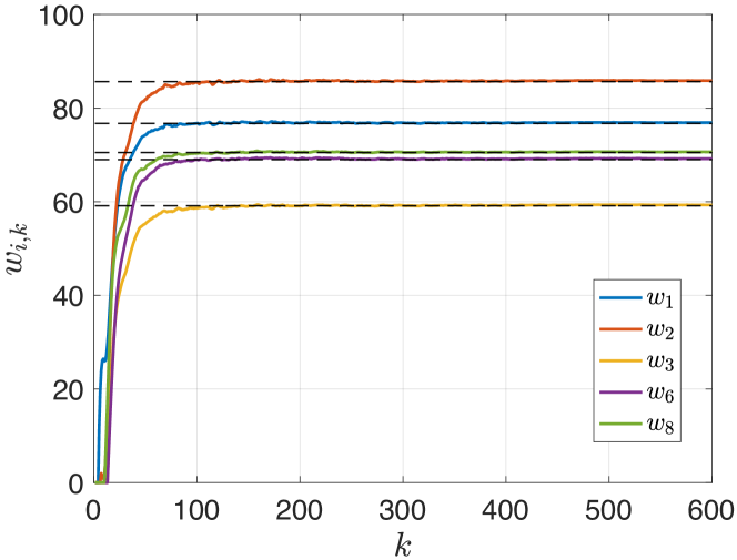
Figure 2: Convergence performance of the generated power from Generators 1, 2, 3, 6, and 8.

Fig. 3 shows that the total generation asymptomatically converges to a neighborhood of the total demand.

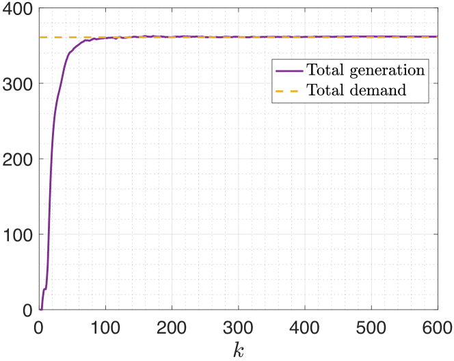
Figure 3: Total generated power and demand.

6.2 Tradeoff between Accuracy and Privacy

To demonstrate the tradeoff between convergence accuracy and the privacy level. We let $\theta_{\xi,0}=\theta_{\zeta,0}=\theta_{0}$, fix $\alpha_{0}=0.015$, $q=0.991$, $q_{\xi}=q_{\zeta}=0.995$, and vary $\theta_{0}$ from $0$ to $0.1$. Due to the randomness of the Laplacian noise, we run the simulation $2000$ times and obtain the empirical mean. Fig. 4 plots $\mathbb{E}\left[\|\mathbf{w}_{\infty}-\mathbf{w}^{*}\|^{2}\right]$ and $\frac{1}{\theta_{0}}$ under different intense of Laplacian noise, where the latter represents the trend of $\epsilon$. Roughly speaking, Fig. 4 shows that as $\theta_{0}$ increases, the expected convergence error $\mathbb{E}\left[\|\mathbf{w}_{\infty}-\mathbf{w}^{*}\|^{2}\right]$ increases. Moreover, as $\theta_{0}$ increases, $\epsilon$ increases as well. Thus, the tradeoff between the privacy level and the convergence is illustrated.

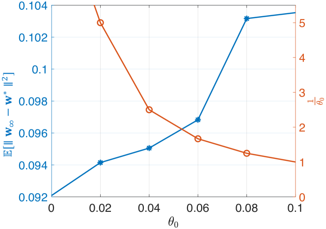
Figure 4: Variations of $\mathbb{E}\left[\|\mathbf{w}_{\infty}-\mathbf{w}^{*}\|^{2}\right]$ and the trend of $\epsilon$ with different noise intensity $\theta_{0}$.

6.3 Comparison with State-of-the-art

We further compare the proposed algorithm with the conventional distributed dual gradient tracking algorithm (DDGT) expressed as (9) in [7] and the differentially private distributed resource allocation via deviation tracking algorithm (diff-DRADT) in Ding et al. [14]. The step size and the noise is set to $\alpha_{k}=0.034\times 0.99^{k}$ and $\theta_{\xi,k}=\theta_{\zeta,k}=0.01\times 0.995^{k}$, respectively. Since there is no privacy preservation in conventional DDGT, to be fair, we run it with the same noise parameter and let $\iota\beta_{k}=\alpha_{k}=0.034\times 0.99^{k}$. Specifically, we set $\beta_{k}=0.99^{k}$ and $\iota=0.034$. Ding et al. [14] used the constant step size and linearly decreasing noise to achieve the finite cumulative privacy loss. Hence, we set the noise the same as ours and set the step size as 0.015.

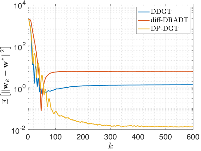
Figure 5: Comparison of our proposed algorithm with the conventional DDGT algorithm [7] with the same privacy level and the diff-DRADT in Ding et al. [14].

Fig. 5 depicts the comparison results. Since diff-DRADT only considers undirected graphs, it suffers from a high optimization error in the directed graph. Due to the lack of robustness, directly adding noise in DDGT will cause noise accumulation and accuracy compromise. It can be seen that under the same noise, our algorithm achieves the best convergence accuracy.

7 Conclusion and Future Work

This paper investigates privacy preservation in distributed resource allocation problems over directed unbalanced networks. We propose a novel differentially private distributed deviation tracking algorithm that incorporates noises into transmitted messages to ensure privacy. The distribution of noise and step sizes are carefully designed to guarantee convergence and achieve $\epsilon$-differential privacy simultaneously.

Potential future research directions include exploring methods to relax the step size requirement and accelerate convergence. Another interesting topic is to deal with the tradeoff between convergence accuracy and privacy level.

Appendix A Appendix

A.1 Preliminary Lemma

Lemma 5.

[32] Let $\{u_{k}\}$, $\{v_{k}\}$, $\{w_{k}\}$ and $\{z_{k}\}$ be the nonnegative sequences of random variables. If they satisfy

$$\mathbb{E}[u_{k+1}]\leq(1+z_{k})u_{k}-v_{k}+w_{k},$$

$$\sum_{k=0}^{\infty}z_{k}<\infty\ a.s.,\ \text{and}\ \sum_{k=0}^{\infty}w_{k}<\infty\ a.s.,$$

then $u_{k}$ converges almost surely (a.s.) to a finite value, and $\sum_{k=0}^{\infty}v_{k}<\infty$ a.s..

A.2 Proof of Lemma 4.8

We aim to prove the component-wise inequalities in (18). To simplify the presentation, we replace the notations $I_{N}$ and $\mathbf{1}_{N}$ as $I$ and $\mathbf{\mathbf{1}}$, respectively.

i) Bound $\mathbb{E}\left[\left\|\mathbf{x}_{k}-\mathbf{1}\bar{\mathbf{x}}_{k}^{T}\right\|^{2}_{R}\big{|}\mathcal{F}_{k}\right]$ and obtain the first inequality:

From (4.1), we can derive that

$$\mathbf{x}_{k+1}-\mathbf{1}\bar{\mathbf{x}}_{k+1}^{T}$$

$$= (\mathbf{R}_{\phi}-\mathbf{1}\pi_{\mathbf{R}}^{T})(\mathbf{x}_{k}-\mathbf{1}\bar{\mathbf{x}}_{k}^{T})-(I-\mathbf{1}\pi_{\mathbf{R}}^{T})\mathbf{v}_{k}$$

$$-\phi(I-\mathbf{1}\pi_{\mathbf{R}}^{T})\mathbf{R}\bm{\zeta}_{k}-\gamma(I-\mathbf{1}\pi_{\mathbf{R}}^{T})\mathbf{C}\bm{\xi}_{k}.$$

Therefore, we have

$$\mathbb{E}\left[\left\|\mathbf{x}_{k+1}-\mathbf{1}\bar{\mathbf{x}}_{k+1}^{T}\right\|^{2}_{R}\big{|}\mathcal{F}_{k}\right]$$

$$= \sigma_{R}^{2}\left\|\mathbf{x}_{k}-\mathbf{1}\bar{\mathbf{x}}_{k}^{T}\right\|^{2}_{R}+\left\|I-\mathbf{1}\pi_{\mathbf{R}}^{T}\right\|_{R}^{2}\mathbb{E}\left[\left\|\mathbf{v}_{k}\right\|_{R}^{2}\big{|}\mathcal{F}_{k}\right]$$

$$+2\sigma_{R}\left\|I-\mathbf{1}\pi_{\mathbf{R}}^{T}\right\|_{R}\left\|\mathbf{x}_{k}-\mathbf{1}\bar{\mathbf{x}}_{k}^{T}\right\|_{R}\left\|\mathbf{v}_{k}\right\|_{R}$$

$$+\phi^{2}\left\|\mathbf{R}-\mathbf{1}\pi_{\mathbf{R}}^{T}\right\|^{2}_{R}\mathbb{E}\left[\left\|\bm{\zeta}_{k}\right\|^{2}_{R}\right]$$

$$+\gamma^{2}\left\|(I-\mathbf{1}\pi_{\mathbf{R}}^{T})\mathbf{C}\right\|^{2}_{R}\mathbb{E}[\left\|\bm{\xi}_{k}\right\|^{2}_{R}]$$

$$\leq \frac{1+\sigma_{R}^{2}}{2}\left\|\mathbf{x}_{k}-\mathbf{1}\bar{\mathbf{x}}_{k}^{T}\right\|^{2}_{R}$$

$$+\frac{1+\sigma_{R}^{2}}{1-\sigma_{R}^{2}}\left\|I-\mathbf{1}\pi_{\mathbf{R}}^{T}\right\|_{R}^{2}\mathbb{E}\left[\left\|\mathbf{v}_{k}\right\|_{R}^{2}\big{|}\mathcal{F}_{k}\right]$$

$$+\phi^{2}Nm\left\|\mathbf{R}-\mathbf{1}\pi_{\mathbf{R}}^{T}\right\|^{2}_{R}\theta_{\zeta,k}^{2}$$

$$+\gamma^{2}Nm\left\|(I-\mathbf{1}\pi_{\mathbf{R}}^{T})\mathbf{C}\right\|^{2}_{R}\theta_{\xi,k}^{2},$$ (39)

where the equality is based on the dependence of the added noise and Lemma 4.6. For the second term, we have

$$\left\|\mathbf{v}_{k}\right\|_{R}^{2}= \left\|\mathbf{v}_{k}-\pi_{\mathbf{C}}\hat{\mathbf{v}}_{k}^{T}+\pi_{\mathbf{C}}\hat{\mathbf{v}}_{k}^{T}\right\|_{R}^{2}$$

$$\leq 2\delta_{R,C}\left\|\mathbf{v}_{k}-\pi_{\mathbf{C}}\hat{\mathbf{v}}_{k}^{T}\right\|_{C}^{2}+2\left\|\pi_{\mathbf{C}}\right\|_{R}^{2}\left\|\hat{\mathbf{v}}_{k}^{T}\right\|_{R}^{2},$$ (40)

and

$$\left\|\hat{\mathbf{v}}_{k}^{T}\right\|_{R}^{2}$$

$$= \left\|\alpha_{k}\mathbf{1}^{T}G(\mathbf{x}_{k})-\alpha_{k}\mathbf{1}^{T}G(\mathbf{1}\bar{\mathbf{x}}_{k}^{T})+\alpha_{k}\mathbf{1}^{T}G(\mathbf{1}\bar{\mathbf{x}}_{k}^{T})\right\|_{R}^{2}$$

$$\leq 2L^{2}N\alpha_{k}^{2}\left\|\mathbf{x}_{k}-\mathbf{1}\bar{\mathbf{x}}_{k}^{T}\right\|_{R}^{2}+2\alpha_{k}^{2}\left\|\nabla f(\bar{\mathbf{x}}_{k})\right\|_{2}^{2},$$ (41)

where the inequality is based on the $L$-Lipschitz smoothness of $f_{i}$. Combining (A.2)–(A.2), we obtain

$$\mathbb{E}\left[\left\|\mathbf{x}_{k+1}-\mathbf{1}\bar{\mathbf{x}}_{k+1}^{T}\right\|^{2}_{R}\big{|}\mathcal{F}_{k}\right]$$

$$\leq \left(\frac{1+\sigma_{R}^{2}}{2}+\mathbf{a}_{1}\alpha_{k}^{2}\right)\left\|\mathbf{x}_{k}-\mathbf{1}\bar{\mathbf{x}}_{k}^{T}\right\|^{2}_{R}$$

$$+2\frac{1+\sigma_{R}^{2}}{1-\sigma_{R}^{2}}\left\|I_{N}-\mathbf{1}\pi_{\mathbf{R}}^{T}\right\|_{R}^{2}\delta_{R,C}^{2}\left\|\mathbf{v}_{k}-\pi_{\mathbf{C}}\hat{\mathbf{v}}_{k}^{T}\right\|_{\mathbf{C}}^{2}$$

$$+4\frac{1+\sigma_{R}^{2}}{1-\sigma_{R}^{2}}\left\|I_{N}-\mathbf{1}\pi_{\mathbf{R}}^{T}\right\|_{R}^{2}\left\|\pi_{\mathbf{C}}\right\|_{R}^{2}\alpha_{k}^{2}\mathbb{E}[\left\|\nabla f(\bar{\mathbf{x}}_{k})\right\|_{2}^{2}]$$

$$+\phi^{2}Nm\left\|\mathbf{R}-\mathbf{1}\pi_{\mathbf{R}}^{T}\right\|_{R}^{2}\theta_{\zeta,k}^{2}$$

$$+\gamma^{2}Nm\left\|(I-\mathbf{1}\pi_{\mathbf{R}}^{T})\mathbf{C}\right\|_{R}^{2}\theta_{\xi,k}^{2}.$$ (42)

ii) Bound $\mathbb{E}\left[\left\|\mathbf{v}_{k}-\pi_{\mathbf{C}}\hat{\mathbf{v}}_{k}^{T}\right\|_{C}^{2}\big{|}\mathcal{F}_{k}\right]$ and get the second inequality:

From (16), we can obtain that

$$\mathbf{v}_{k+1}-\pi_{\mathbf{C}}\hat{\mathbf{v}}_{k+1}^{T}$$

$$= (\mathbf{C}_{\gamma}-\pi_{\mathbf{C}}\mathbf{1}^{T})(\mathbf{v}_{k}-\pi_{\mathbf{C}}\hat{\mathbf{v}}_{k}^{T})+(I-\pi_{\mathbf{C}})\mathbf{v}_{k+1}$$

$$-(\mathbf{C}_{\gamma}-\pi_{\mathbf{C}}\mathbf{1}^{T})\mathbf{v}_{k}$$

$$= (\mathbf{C}_{\gamma}-\pi_{\mathbf{C}}\mathbf{1}^{T})(\mathbf{v}_{k}-\pi_{\mathbf{C}}\hat{\mathbf{v}}_{k}^{T})-(\mathbf{C}_{\gamma}-\pi_{\mathbf{C}}\mathbf{1}^{T})\mathbf{v}_{k}$$

$$+(I-\pi_{\mathbf{C}}\mathbf{1}^{T})[(\mathbf{C}_{\gamma}-I)\mathbf{y}_{k+1}+\alpha_{k+1}G(\mathbf{x}_{k+1})]$$

$$= (\mathbf{C}_{\gamma}-\pi_{\mathbf{C}}\mathbf{1}^{T})(\mathbf{v}_{k}-\pi_{\mathbf{C}}\hat{\mathbf{v}}_{k}^{T})+(I-\pi_{\mathbf{C}}\mathbf{1}^{T})\alpha_{k+1}G(\mathbf{x}_{k+1})$$

$$-(\mathbf{C}_{\gamma}-\pi_{\mathbf{C}}\mathbf{1}^{T})[(\mathbf{C}_{\gamma}-I)\mathbf{y}_{k}+\alpha_{k}G(\mathbf{x}_{k})]$$

$$+(I-\pi_{\mathbf{C}}\mathbf{1}^{T})(\mathbf{C}_{\gamma}-I)(\mathbf{C}_{\gamma}\mathbf{y}_{k}+\alpha_{k}G(\mathbf{x}_{k})+\gamma\mathbf{C}\bm{\xi}_{k})$$

$$= (\mathbf{C}_{\gamma}-\pi_{\mathbf{C}}\mathbf{1}^{T})(\mathbf{v}_{k}-\pi_{\mathbf{C}}\hat{\mathbf{v}}_{k}^{T})$$

$$+(I-\pi_{\mathbf{C}}\mathbf{1}^{T})(\alpha_{k+1}G(\mathbf{x}_{k+1})-\alpha_{k}G(\mathbf{x}_{k}))+\gamma(\mathbf{C}_{\gamma}-I)\mathbf{C}\bm{\xi}_{k}.$$

Therefore, we have

$$\mathbb{E}\left[\left\|\mathbf{v}_{k+1}-\pi_{\mathbf{C}}\hat{\mathbf{v}}_{k+1}^{T}\right\|_{C}^{2}\big{|}\mathcal{F}_{k}\right]$$

$$\leq \frac{1+\sigma_{C}^{2}}{2}\left\|\mathbf{v}_{k}-\pi_{\mathbf{C}}\hat{\mathbf{v}}_{k}^{T}\right\|_{C}^{2}$$

$$+\frac{1+\sigma_{C}^{2}}{1-\sigma_{C}^{2}}\left\|I_{N}-\pi_{\mathbf{C}}\mathbf{1}^{T}\right\|_{C}^{2}\mathbb{E}\big{[}\left\|\alpha_{k+1}G(\mathbf{x}_{k+1})-\alpha_{k}G(\mathbf{x}_{k})\right.$$

$$+\left.\gamma(\mathbf{C}_{\gamma}-I)\mathbf{C}\bm{\xi}_{k}\right\|_{C}^{2}\big{]}$$

$$\leq \frac{1+\sigma_{C}^{2}}{2}\left\|\mathbf{v}_{k}-\pi_{\mathbf{C}}\hat{\mathbf{v}}_{k}^{T}\right\|_{C}^{2}$$

$$+\frac{1+\sigma_{C}^{2}}{1-\sigma_{C}^{2}}\left\|I_{N}-\pi_{\mathbf{C}}\mathbf{1}^{T}\right\|_{C}^{2}\mathbb{E}\left[\left\|\alpha_{k+1}G(\mathbf{x}_{k+1})-\alpha_{k}G(\mathbf{x}_{k})\right\|_{C}^{2}\right]$$

$$+2\frac{1+\sigma_{C}^{2}}{1-\sigma_{C}^{2}}\left\|I_{N}-\pi_{\mathbf{C}}\mathbf{1}^{T}\right\|_{C}^{2}\mathbb{E}\left[\|\gamma(\mathbf{C}_{\gamma}-I)C\bm{\xi}_{k}\|_{C}^{2}\right].$$ (43)

For the third term of (A.2), we have

$$\mathbb{E}[\gamma(\alpha_{k+1}G(\mathbf{x}_{k+1})-\alpha_{k}G(\mathbf{x}_{k}))^{T}(\mathbf{C}_{\gamma}-I)C\bm{\xi}_{k}|\mathcal{F}_{k}]$$

$$= \mathbb{E}[\gamma\alpha_{k+1}G(\mathbf{x}_{k+1})^{T}(\mathbf{C}_{\gamma}-I)C\bm{\xi}_{k}|\mathcal{F}_{k}]$$

$$= \mathbb{E}[\gamma\alpha_{k+1}G(\mathbf{R}_{\phi}\mathbf{x}_{k}-\mathbf{v}_{k}-\phi\mathbf{R}\bm{\zeta}_{k}-\gamma\mathbf{C}\bm{\xi}_{k})^{T}(\mathbf{C}_{\gamma}-I)C\bm{\xi}_{k}|\mathcal{F}_{k}]$$

$$\leq 2\gamma^{2}LNm\alpha_{k+1}\|\mathbf{C}\|\|(\mathbf{C}_{\gamma}-I)\mathbf{C}\|\theta_{\xi,k}^{2},$$ (44)

where the inequality is from $\mathbb{E}[\gamma\alpha_{k+1}G(\mathbf{R}_{\phi}\mathbf{x}_{k}-\mathbf{v}_{k}-\phi\mathbf{R}\bm{\zeta}_{k}-\gamma\mathbf{C}\bm{\xi}_{k})^{T}(\mathbf{C}_{\gamma}-I)C\bm{\xi}_{k}|\mathcal{F}_{k}]=\gamma\alpha_{k+1}\mathbb{E}[(G(\mathbf{R}_{\phi}\mathbf{x}_{k}-\mathbf{v}_{k}-\phi\mathbf{R}\bm{\zeta}_{k}-\gamma\mathbf{C}\bm{\xi}_{k})-G(\mathbf{R}_{\phi}\mathbf{x}_{k}-\mathbf{v}_{k}-\phi\mathbf{R}\bm{\zeta}_{k})+G(\mathbf{R}_{\phi}\mathbf{x}_{k}-\mathbf{v}_{k}-\phi\mathbf{R}\bm{\zeta}_{k}))^{T}(\mathbf{C}_{\gamma}-I)C\bm{\xi}_{k}|\mathcal{F}_{k}]=\mathbb{E}[(G(\mathbf{R}_{\phi}\mathbf{x}_{k}-\mathbf{v}_{k}-\phi\mathbf{R}\bm{\zeta}_{k}-\gamma\mathbf{C}\bm{\xi}_{k})-G(\mathbf{R}_{\phi}\mathbf{x}_{k}-\mathbf{v}_{k}-\phi\mathbf{R}\bm{\zeta}_{k}))^{T}(\mathbf{C}_{\gamma}-I)C\bm{\xi}_{k}|\mathcal{F}_{k}]$ and the $L$-Lipschitzness of $f_{i}$. Furthermore, we have $\left\|\alpha_{k+1}G(\mathbf{x}_{k+1})-\alpha_{k}G(\mathbf{x}_{k+1})\right\|_{C}^{2}\leq L^{2}\max\{\alpha_{k+1}^{2},\alpha_{k}^{2}\}\left\|\mathbf{x}_{k+1}-\mathbf{x}_{k}\right\|_{C}^{2}$. For $\|\mathbf{x}_{k+1}-\mathbf{x}_{k}\|_{C}^{2}$, we first derive

$$\mathbf{x}_{k+1}-\mathbf{x}_{k}$$

$$= (\mathbf{R}_{\gamma}-I)(\mathbf{x}_{k}-\mathbf{1}\bar{\mathbf{x}}_{k}^{T})-(\mathbf{v}_{k}-\pi_{\mathbf{C}}\hat{\mathbf{v}}_{k}^{T})-\pi_{\mathbf{C}}\hat{\mathbf{v}}_{k}^{T}$$

$$+\phi\mathbf{R}\bm{\zeta}_{k}-\gamma\mathbf{C}\bm{\xi}_{k},$$

and then,

$$\mathbb{E}\left[\left\|\mathbf{x}_{k+1}-\mathbf{x}_{k}\right\|_{C}^{2}|\mathcal{F}_{k}\right]$$

$$\leq 3\left\|\mathbf{R}_{\gamma}-I\right\|_{C}^{2}\left\|\mathbf{x}_{k}-\mathbf{1}\bar{\mathbf{x}}_{k}^{T}\right\|_{C}^{2}+3\left\|\mathbf{v}_{k}-\pi_{\mathbf{C}}\hat{\mathbf{v}}_{k}^{T}\right\|_{\mathbf{C}}^{2}$$

$$+3\left\|\pi_{\mathbf{C}}\right\|_{C}^{2}\left\|\hat{\mathbf{v}}_{k}^{T}\right\|_{C}^{2}+\phi^{2}\left\|\mathbf{R}\right\|_{C}^{2}Nm\theta_{\zeta,k}^{2}$$

$$+\gamma^{2}\left\|\mathbf{C}\right\|_{C}^{2}Nm\theta_{\xi,k}^{2}$$

$$\leq 3\sigma_{C,R}^{2}\left[\left\|\mathbf{R}_{\gamma}-I\right\|_{C}^{2}+2L^{2}N\alpha_{k}^{2}\left\|\pi_{\mathbf{C}}\right\|_{C}^{2}\right]\left\|\mathbf{x}_{k}-\mathbf{1}\bar{\mathbf{x}}_{k}^{T}\right\|_{R}^{2}$$

$$+3\left\|\mathbf{v}_{k}-\pi_{\mathbf{C}}\hat{\mathbf{v}}_{k}^{T}\right\|_{\mathbf{C}}^{2}+6\left\|\pi_{\mathbf{C}}\right\|_{C}^{2}\sigma_{C,R}^{2}\alpha_{k}^{2}\mathbb{E}[\left\|\nabla f(\bar{\mathbf{x}}_{k})\right\|_{2}^{2}]$$

$$+\phi^{2}\left\|\mathbf{R}\right\|_{C}^{2}Nm\theta_{\zeta,k}^{2}+\gamma^{2}\left\|\mathbf{C}\right\|_{C}^{2}Nm\theta_{\xi,k}^{2}.$$ (45)

Combining (A.2)–(A.2) , we have

$$\mathbb{E}[\left\|\mathbf{v}_{k+1}-\pi_{\mathbf{C}}\hat{\mathbf{v}}_{k+1}^{T}\right\|_{C}^{2}]$$ (46)

$$\leq \left(\frac{1+\sigma_{C}^{2}}{2}+\mathbf{a}_{5}\max\{\alpha_{k+1}^{2},\alpha_{k}^{2}\}\right)\left\|\mathbf{v}_{k+1}-\pi_{\mathbf{C}}\hat{\mathbf{v}}_{k+1}^{T}\right\|_{C}^{2}$$

$$+(\mathbf{a}_{3}+\mathbf{a}_{4}\alpha_{k}^{2})\max\{\alpha_{k+1}^{2},\alpha_{k}^{2}\}\left\|\mathbf{x}_{k}-\mathbf{1}\bar{\mathbf{x}}_{k}^{T}\right\|_{R}^{2}$$

$$+B_{21}\alpha_{k}^{2}\max\{\alpha_{k+1}^{2},\alpha_{k}^{2}\}\mathbb{E}[\left\|\nabla f(\bar{\mathbf{x}}_{k})\right\|_{2}^{2}]$$

$$+B_{22}\max\{\alpha_{k+1}^{2},\alpha_{k}^{2}\}\phi^{2}\theta_{\zeta,k}^{2}+B_{23}\gamma^{2}\theta_{\xi,k}^{2}.$$ (47)

A.3 Proof of Corollary 5.14

First, for the step size and noise given in Corollary 5.14, we have $\sum_{k=0}^{\infty}\theta_{\xi,k}^{2}=\theta_{\xi,0}^{2}\sum_{k=0}^{\infty}q_{\xi}^{2k}=\frac{\theta_{\xi,0}^{2}}{1-q_{\xi}}<\infty$, $\sum_{k=0}^{\infty}\theta_{\zeta,k}^{2}=\theta_{\zeta,0}^{2}\sum_{k=0}^{\infty}q_{\zeta}^{2k}=\frac{\theta_{\zeta,0}^{2}}{1-q_{\zeta}}<\infty$, $\sum_{k=0}^{\infty}\alpha_{k}=\alpha_{0}\sum_{k=0}^{\infty}q^{k}=\frac{\alpha_{0}}{1-q}<\infty$, $\sum_{k=0}^{\infty}\frac{\theta_{\xi,k}^{2}}{\alpha_{k}}=\frac{\theta_{\xi,0}^{2}}{\alpha_{0}}\sum_{k=0}^{\infty}\left(\frac{q_{\xi}^{2}}{q}\right)^{k}=\frac{\theta_{\xi,0}^{2}q}{\alpha_{0}(q-q_{\xi}^{2})}<\infty$, and $\sum_{k=0}^{\infty}\frac{\theta_{\zeta,k}^{2}}{\alpha_{k}}=\frac{\theta_{\zeta,0}^{2}}{\alpha_{0}}\sum_{k=0}^{\infty}\left(\frac{q_{\zeta}^{2}}{q}\right)^{k}=\frac{\theta_{\zeta,0}^{2}q}{\alpha_{0}(q-q_{\zeta}^{2})}<\infty$, which satisfies sufficient conditions in Theorem 4.11. Therefore, under DP-DGT, $\|\mathbf{w}_{k}-\mathbf{w}^{*}\|^{2}$ is stochastically bounded.

Then, we consider two non-decreasing nonnegative sequence $\{\varphi_{k}^{\prime}\}$ and $\{\eta_{k}^{\prime}\}$, iteratively evolving as follows:

$$\varphi_{k+1}^{\prime} =\varphi_{k}^{\prime}+\frac{\alpha}{\mu}\eta_{k}^{\prime}+\frac{\alpha\delta}{\mu},$$ (48)

$$\eta_{k+1}^{\prime} =2\varphi_{k}^{\prime}+\eta_{k}^{\prime}+\frac{\alpha}{\mu}\eta_{k}^{\prime}+\frac{\alpha\delta}{\mu},$$

with $\varphi_{0}^{\prime}=0$ and $\eta_{0}^{\prime}=0$. Then, we have $\varphi_{k}\leq\varphi_{k}^{\prime}$ and $\eta_{k}\leq\eta_{k}^{\prime}$ according to (32). Based on (48), $\varphi_{k+1}^{\prime}=\frac{\alpha}{\mu}\sum_{t=0}^{k}\eta_{t}^{\prime}+\frac{\alpha\delta}{\mu}(k+1)\leq\frac{\alpha}{\mu}(\delta+\eta_{k}^{\prime})(k+1)$, and thus $\varphi_{k}^{\prime}\leq\frac{\alpha}{\mu}(\delta+\eta_{k}^{\prime})k$. Hence, $\eta_{k}^{\prime}$ is increasing with $k$, indicating that $D_{\eta}$ is increasing with $K$.

Under the conditions listed in Corollary 5.14, one has $\bar{\alpha}=\alpha_{0}$, $k_{0}=0$, and $K=0$. Therefore, we derive that $D_{\eta}=\frac{2\alpha_{0}\delta}{\gamma\phi\mu-\alpha_{0}}$. Additionally, we have $D_{\alpha,\xi}=\frac{\alpha_{0}q_{\xi}}{\theta_{\xi,0}(q_{\xi}-q)}$ and $D_{\alpha,\zeta}=\frac{\alpha_{0}q_{\zeta}}{\theta_{\zeta,0}(q_{\zeta}-q)}$. Therefore, we obtain that

$$\epsilon=\frac{\alpha_{0}\delta(\gamma\phi\mu+\alpha_{0})}{\gamma\phi\mu(\gamma\phi\mu-\alpha_{0})}\left(\frac{q_{\xi}}{\theta_{\xi,0}(q_{\xi}-q)}+\frac{\phi q_{\zeta}}{\theta_{\zeta,0}(q_{\zeta}-q)}\right).$$

References

• [1] Tao Yang, Jie Lu, Di Wu, Junfeng Wu, Guodong Shi, Ziyang Meng, and Karl Henrik Johansson. A distributed algorithm for economic dispatch over time-varying directed networks with delays. IEEE Transactions on Industrial Electronics, 64(6):5095–5106, 2016.
• [2] Lin Xiao, Mikael Johansson, and Stephen P Boyd. Simultaneous routing and resource allocation via dual decomposition. IEEE Transactions on Communications, 52(7):1136–1144, 2004.
• [3] Allen J Wood, Bruce F Wollenberg, and Gerald B Sheblé. Power Generation, Operation, and Control. John Wiley & Sons, 2013.
• [4] Tao Guo, Mark I Henwood, and Marieke Van Ooijen. An algorithm for combined heat and power economic dispatch. IEEE Transactions on Power Systems, 11(4):1778–1784, 1996.
• [5] Ziang Zhang and Mo-Yuen Chow. Convergence analysis of the incremental cost consensus algorithm under different communication network topologies in a smart grid. IEEE Transactions on Power Systems, 27(4):1761–1768, 2012.
• [6] Peng Yi, Yiguang Hong, and Feng Liu. Initialization-free distributed algorithms for optimal resource allocation with feasibility constraints and application to economic dispatch of power systems. Automatica, 74:259–269, 2016.
• [7] Jiaqi Zhang, Keyou You, and Kai Cai. Distributed dual gradient tracking for resource allocation in unbalanced networks. IEEE Transactions on Signal Processing, 68:2186–2198, 2020.
• [8] Nikolaos M Freris and Panagiotis Patrinos. Distributed computing over encrypted data. In 54th Annual Allerton Conference on Communication, Control, and Computing, pages 1116–1122, 2016.
• [9] Cynthia Dwork. Differential privacy. In International colloquium on automata, languages, and programming, pages 1–12. Springer, 2006.
• [10] Xiaomeng Chen, Lingying Huang, Lidong He, Subhrakanti Dey, and Ling Shi. A differentially private method for distributed optimization in directed networks via state decomposition. IEEE Transactions on Control of Network Systems, 2023.
• [11] Yongqiang Wang and Angelia Nedić. Tailoring gradient methods for differentially-private distributed optimization. IEEE Transactions on Automatic Control, 2023.
• [12] Lingying Huang, Junfeng Wu, Dawei Shi, Subhrakanti Dey, and Ling Shi. Differential privacy in distributed optimization with gradient tracking. IEEE Transactions on Automatic Control, 2024.
• [13] Shuo Han, Ufuk Topcu, and George J Pappas. Differentially private distributed constrained optimization. IEEE Transactions on Automatic Control, 62(1):50–64, 2016.
• [14] Tie Ding, Shanying Zhu, Cailian Chen, Jinming Xu, and Xinping Guan. Differentially private distributed resource allocation via deviation tracking. IEEE Transactions on Signal and Information Processing over Networks, 7:222–235, 2021.
• [15] Wenwen Wu, Shanying Zhu, Shuai Liu, and Xinping Guan. Differentially private distributed mismatch tracking algorithm for constraint-coupled resource allocation problems. In IEEE 61st Conference on Decision and Control, pages 3965–3970, 2022.
• [16] Dimitri P Bertsekas. Nonlinear programming. Journal of the Operational Research Society, 48(3):334–334, 1997.
• [17] Xingyu Zhou. On the fenchel duality between strong convexity and lipschitz continuous gradient. arXiv preprint arXiv:1803.06573, 2018.
• [18] Stephen P Boyd and Lieven Vandenberghe. Convex Optimization. Cambridge University Press, 2004.
• [19] Shi Pu, Wei Shi, Jinming Xu, and Angelia Nedić. Push–pull gradient methods for distributed optimization in networks. IEEE Transactions on Automatic Control, 66(1):1–16, 2020.
• [20] Konstantinos I Tsianos, Sean Lawlor, and Michael G Rabbat. Push-sum distributed dual averaging for convex optimization. In IEEE 51st Conference on Decision and Control, pages 5453–5458, 2012.
• [21] Chenguang Xi and Usman A Khan. Dextra: A fast algorithm for optimization over directed graphs. IEEE Transactions on Automatic Control, 62(10):4980–4993, 2017.
• [22] Zhenqi Huang, Sayan Mitra, and Nitin Vaidya. Differentially private distributed optimization. In Proceedings of the 16th International Conference on Distributed Computing and Networking, pages 1–10, 2015.
• [23] Soummya Kar and Gabriela Hug. Distributed robust economic dispatch in power systems: A consensus+ innovations approach. In IEEE Power and Energy Society General Meeting, pages 1–8, 2012.
• [24] Qingguo Lü, Shaojiang Deng, Huaqing Li, and Tingwen Huang. Privacy protection decentralized economic dispatch over directed networks with accurate convergence. IEEE Transactions on Emerging Topics in Computational Intelligence, 2023.
• [25] Yongqiang Wang and Tamer Başar. Quantization enabled privacy protection in decentralized stochastic optimization. IEEE Transactions on Automatic Control, 68(7):4038–4052, 2023.
• [26] Wei-Ning Chen, Christopher A Choquette Choo, Peter Kairouz, and Ananda Theertha Suresh. The fundamental price of secure aggregation in differentially private federated learning. In International Conference on Machine Learning, pages 3056–3089, 2022.
• [27] Shi Pu. A robust gradient tracking method for distributed optimization over directed networks. In 59th IEEE Conference on Decision and Control, pages 2335–2341, 2020.
• [28] Tie Ding, Shanying Zhu, Jianping He, Cailian Chen, and Xinping Guan. Differentially private distributed optimization via state and direction perturbation in multiagent systems. IEEE Transactions on Automatic Control, 67(2):722–737, 2021.
• [29] Roger A Horn and Charles R Johnson. Matrix Analysis. Cambridge University Press, 2012.
• [30] Alex Q Huang, Mariesa L Crow, Gerald Thomas Heydt, Jim P Zheng, and Steiner J Dale. The future renewable electric energy delivery and management (FREEDM) system: the energy internet. Proceedings of the IEEE, 99(1):133–148, 2010.
• [31] Shiping Yang, Sicong Tan, and Jian-Xin Xu. Consensus based approach for economic dispatch problem in a smart grid. IEEE Transactions on Power Systems, 28(4):4416–4426, 2013.
• [32] Herbert Robbins and David Siegmund. A convergence theorem for nonnegative almost supermartingales and some applications. In Optimizing Methods in Statistics, pages 233–257. 1971.