Non-Hermitian Topology with Generalized Chiral Symmetry
Abstract
We study a generalization of chiral symmetry applicable to non-Hermitian systems and its topological consequences on one-dimensional chains. We uncover a rich family of topological phases hosting several chiral flavors characterized not by a single winding number, but a vector of of them. This, in turn, leads to a novel type of bulk-boundary correspondence, where – in contrast with conventional chiral chains – some flavors can have topologically stable non-zero charges on both ends. Moreover, we find that the total charge of each flavor can in some cases exceed the magnitude of the highest winding number in the vector invariant. Our work extends the topological classification of the non-Hermitian AIII class along a new axis.
I Introduction
The classification and understanding of topological phases in condensed matter physics have been central to unraveling the intricate properties of quantum materials. In recent years, non-Hermitian systems have emerged as a promising avenue for exploration, where phenomena not seen in conventional Hermitian systems challenge the conventional wisdom about topological phases. Perhaps the most prominent example of this is the non-Hermitian skin effect and its effect on the concept of bulk-boundary correspondence (BBC) in topological phases [1, 2, 3, 4].
Since the spectra for non-Hermitian Hamiltonians is with some notable exceptions [5, 6] generally complex, the notion of a spectral gap needs some revision. One typically speaks of two types of gaps in non-Hermitian spectra [7]. The one closest to the Hermitian gap is the line gap, where the spectrum consists of two parts, with each part being on either side of a line going across the complex energy plane. The other type of gap is the point gap, where the spectrum does not necessarily separate into distinct parts, but rather can be found to be at least a minimum distance away from some specific point in the energy plane. Although the existence of a line gap also implies the existence of a point gap, the point gap has no Hermitian analog.
The topological classification of non-Hermitian systems for both line and point gaps is largely captured in the topological periodic table of Bernard-LeClair classes [8, 9, 10, 11, 12, 13] valid for Hamiltonians in any spatial dimension satisfying local symmetries of the form , where , is a unitary matrix acting locally in space, and represents the transpose, Hermitian conjugate, or conjugate of . The classification has then mainly been extended by considering non-local [14, 15].
A hitherto much less explored extension is allowing to take on other values on the unit circle than just . One example of such an extension is a generalized chiral symmetry as introduced for non-interacting fermions in [16], where they proved a generalization of Lieb’s theorem applicable to multipartite systems. This generalized symmetry was subsequently used to construct higher-root topological insulators [17]. Outside of this, the generalized chiral symmetry is also present in Baxter’s clock model for parafermions [16, 18, 19], and a more general version of this symmetry was also shown to allow for the existence of higher-order topological phases in Hermitian systems [20, 21].
In the interest of extending the topological classification of non-Hermitian systems, we dedicate this work to studying the topological properties of one-dimensional chains possessing this generalized chiral symmetry. We will see how it gives rise to a rich set of topological phases with a novel BBC. The remainder of the paper is structured as follows: in Sec. II, we provide a brief introduction to the generalized chiral symmetry. In Sec. III we argue for the presence of topological phases and define the relevant topological invariant. Building on that, we present the BBC in Sec. IV and discuss how it differs from conventional chiral systems. Finally, in Sec. V, we summarize our findings, and discuss some potential future research directions.
II Symmetry Preliminaries
In its standard form, chiral symmetry is expressed as an anticommutation relation between a Hamiltonian and a unitary matrix with the property . The generalized chiral symmetry – from hereon referred to as -chiral symmetry (CS) – modifies these relations in the following way: the anticommutation relation is replaced by
| (1) |
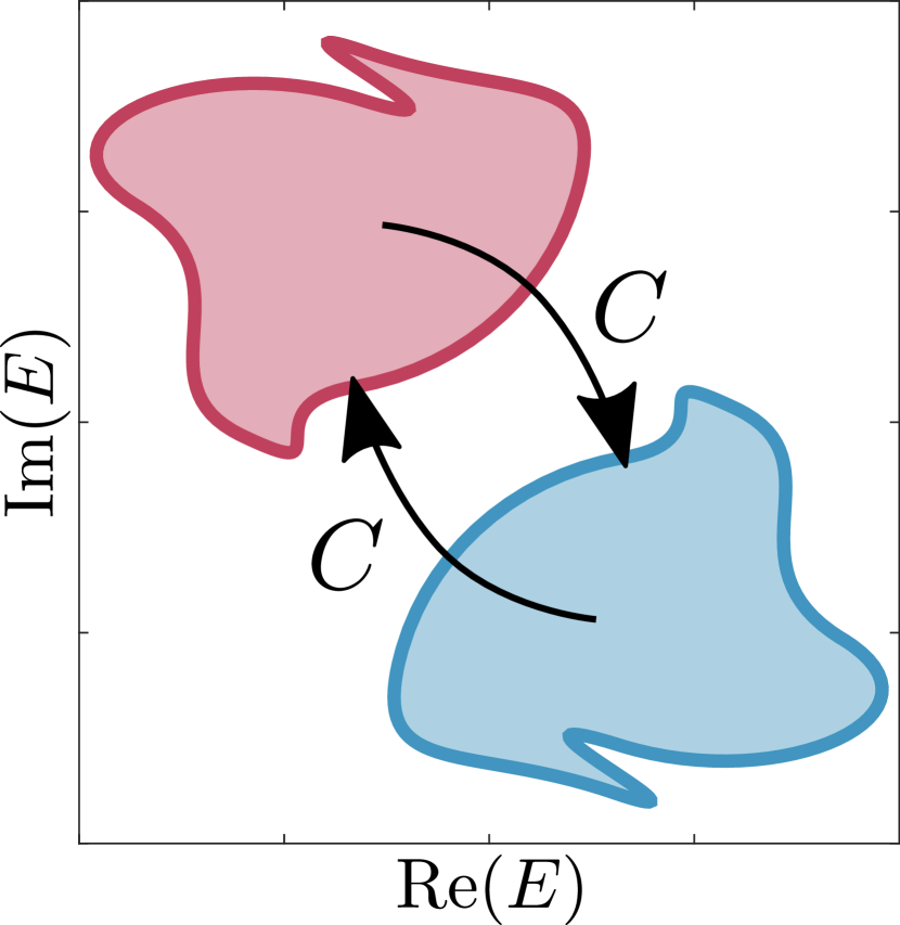
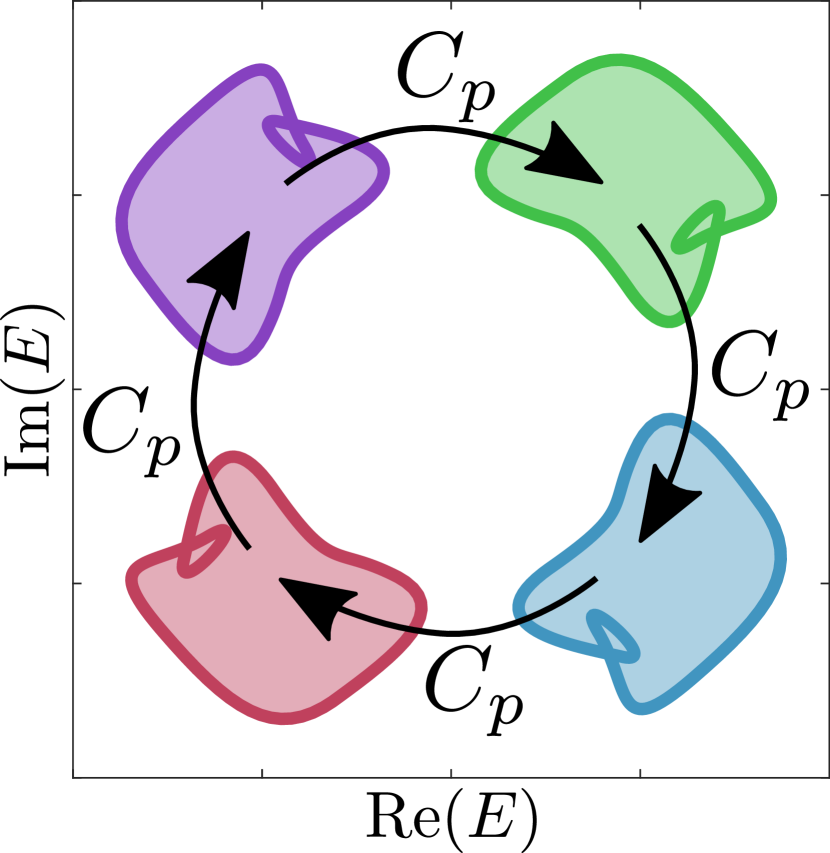
where is a complex phase, and the -chiral operator satisfies , from which it follows that . In this notation, the standard chiral symmetry corresponds to .
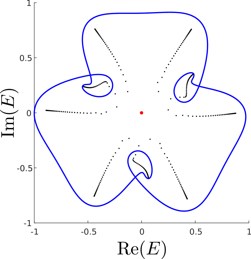
An immediate consequence of CS is that the spectrum will have a rotational symmetry in the complex energy plane; for any eigenstate with eigenvalue , will also be an eigenstate with energy . In fact, repeatedly applying on gives us a -tuple of eigenstates whose energies are related by different powers of . As such, CS for can only be present in systems with complex spectra, so that for the remainder of this paper, we will only concern ourselves with non-Hermitian Hamiltonians. However, we do not exclude the conventional case as it will very much be encompassed by the ensuing discussion. For a schematic picture of typical spectra, see Fig. 1.
Since our focus will be on gapped topological phases (with respect to zero energy), we will assume is of the form
| (2) |
where is the number of additional degrees of freedom. Any other choice of sizes for the different chiral sectors would lead to zero-energy bands as per Lieb’s theorem [16].
Any Hamiltonian possessing CS must in this diagonal basis for the operator be of the form
| (3) |
where each is a -by- matrix. Similarly to the standard chiral symmetry, this form allows us to make a sublattice interpretation, but instead of having only two sublattices, we now have sublattices, that are connected in a cyclic way.
The spectrum for the Hamiltonian in Eq. (3) can be solved from the characteristic equation
| (4) |
where we explicitly see the aforementioned rotational symmetry manifest: if is a solution to the characteristic equation, then for any integer will also satisfy it. The above expression also makes it evident that all individual need to have a gapped spectrum for the system to be gapped.
III Winding and Topology
The topological nature of zero-energy edge modes in systems with conventional chiral symmetry can be understood through the following argument: suppose we have a one-dimensional semi-infinite chain with a single zero-energy boundary mode energetically isolated from the bulk modes, chiral symmetry maps states with energy to states with energy locally, thus the single zero-energy boundary state must be an eigenstate of the chiral operator. In other words, it has an associated chiral charge; conversely, finite-energy states are superpositions of both chiralities. Because of this, we are unable to remove the boundary mode from zero energy without breaking the chiral symmetry or closing the gap. In fact, we can have an arbitrary amount of zero modes at the boundary which can not be removed if they all carry the same chiral charge. However, if we have boundary modes of opposite chiral charge, we can combine them and remove them from zero energy without breaking the symmetry.
In a similar vein, if we have a zero-energy state in a CS system, it will also have an associated chiral charge, and it can also not be removed without either breaking the symmetry, closing the gap, or using zero-energy states of complementary chiral charges. In fact, this already allows us to deduce the first novel feature of CS topology: to gap out a zero mode without breaking symmetry requires the introduction of the other chiral charges by coming into contact with either other zero modes or bulk states. This implies that there will not necessarily be an equal number of states at each end of a finite chain. However, the total charge at each end must equal in magnitude but differ in sign. We will elaborate more on the BBC further down.
Before that, we must first discuss winding numbers. Unlike Hermitian physics, the spectrum for a non-Hermitian system with open boundary conditions (OBC) can be vastly different from that of the corresponding one with periodic boundary conditions (PBC). As it pertains to the setups studied in this article, one can define a spectral winding number (or vorticity) [9, 12]
| (5) |
for a continuous and periodic matrix function , where is the circle and is the set of complex-valued matrices. This winding number can be calculated for any point in the complex energy plane provided it does not coincide with the eigenvalue of for some . The winding number tells us how many times the spectrum winds around said point as we go around the Brillouin zone (BZ). This value is of great relevance, since if it is non-zero, there will be skin modes present at that energy [22, 23, 24] in a semi-infinite chain [25].
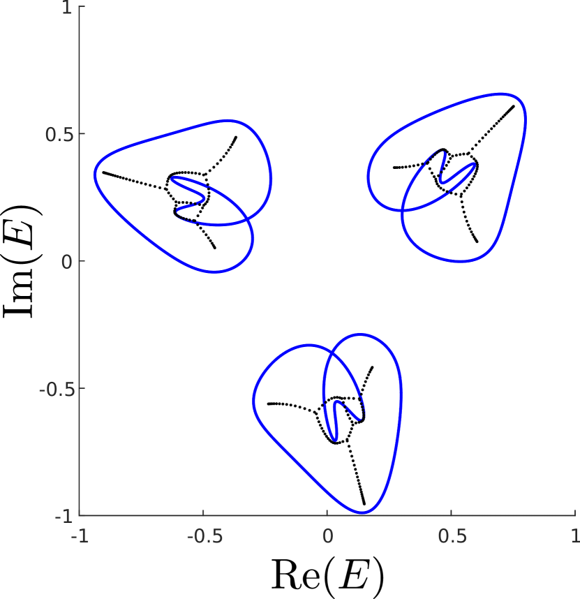
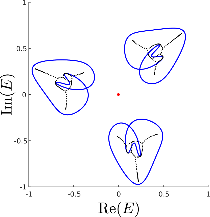
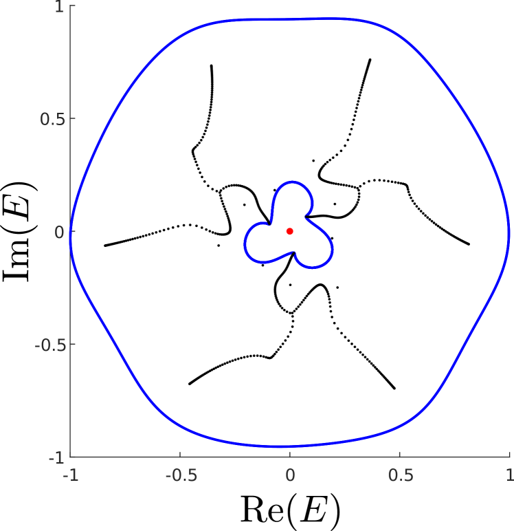
To ensure that our non-Hermitian system remains gapped even when taking skin modes into account, it is then imperative that we restrict ourselves to systems where the winding number around is zero. As shown in App. A, the winding number for a Hamiltonian of the form Eq. (3), is given by the sum of the individual winding numbers of each (here needs to be taken modulo ). However, a topologically non-trivial phase still requires at least some of the winding numbers for the individual blocks to be non-zero, lest there can be no zero-modes. To illustrate this, we show the PBC and OBC spectra for a trivial (topological) CS model in Fig. 2(a) (Fig. 2(b)). In Fig. 2(c), we show an example of a system with non-zero total winding. The randomly generated topologically non-trivial toy model has been constructed using blocks of the form
| (6) |
where and are complex numbers satisfying . This requirement ensures that it traces out a path encircling the origin of the complex plane. Conversely, we constructed the topologically trivial model by inverting the inequality. In either case, Eq. (6) corresponds to an onsite term and an th-order hopping between sites. We generated random and for each block. For the topological phase, we first sampled the modulus of from the unit interval, then we sampled the modulus of from the interval . The phases for each were then sampled from the interval . All sampling was done with uniform distributions.
Note that in all of the plots in Fig. 2, the open-boundary spectrum is extremely sensitive to numerical precision so the specific points in the plotted open-boundary spectra are more suggestive than quantitative. However, we only care about it being confined within the area bounded by the periodic-boundary spectrum, which is always true, so the exact values are not important in this context. The example systems generated here all have spectra that separate into isolated islands, like in the conventional AIII case. However, it is also possible to construct models where the spectrum wraps around the zero-point but such that the total winding remains zero. We present an example of this in App. B. This makes the fact that we are dealing with point-gap spectra all the more obvious.
As per similar logic as for the skin modes, tells us how many zero-energy right eigenstates of the th chiral flavor we have on which side [23]. Simultaneously, it also tells us that we have the same number of zero-energy left eigenstates of the th flavor on the opposite edge. It is this imbalance between left and right eigenvectors and which end they localize on that give rise to a non-trivial BBC. To touch base with something familiar again, we mention that for , it is guaranteed that there are the same amount of left and right eigenstates of the same flavor at either side but with the flavor of one edge being opposite to that of the other. The BBC thus remains unaltered for even when the system is non-Hermitian. We further note that in the Hermitian case, the constraint guarantees that the total winding is zero. Indeed, conventionally, the topological classification for AIII in Hermitian systems is whereas it is in the non-Hermitian case [13], since the winding number of the two blocks become independent. This classification can then immediately be extended to CS where it is given by .
The topological phase for CS systems with vanishing total winding number is then uniquely determined by winding numbers, since the th winding number follows from the aforementioned constraint (the topological classification is accordingly reduced to much like how becomes for conventional AIII when we go from non-Hermitian to Hermitian). In other words, the topological invariant now becomes a vector
| (7) |
where we include all winding numbers for later convenience. We remark that this is still consistent with the conventional chiral symmetry, where the topological invariant is given by the winding of the upper off-diagonal block.
A difference from the Hermitian case, however, is that transitioning between different zero-total-winding (ZTW) phases requires us to change at least two winding numbers, which means that ZTW phases are in general separated by gapless phases, where, again, the gaplessness is defined in terms of the presence of skin modes. This means that in a system where the ZTW spectrum consists of separate islands, the phase transition leads to a transition in the topology of the spectrum as well: as the winding of one block changes, the overall winding becomes non-zero, and we must have at least one spectral band wrapping around zero energy like in Fig. 2(c). This transition between separate islands and one single band happens when the band islands meet and connect at zero energy at the point in parameter space where one block changes winding number. Then as another block changes to a winding number such that the overall winding is zero again, the same procedure happens in reverse. Of course, from this perspective, phase changes for the Hermitian case actually also correspond to changing two winding numbers, but here imposing Hermiticity ensures that the two winding numbers are always opposite to each other.
As a last point of this section, we mention that in the case of a composite for some integers and , one can consider breaking CS into a lower CS corresponding to the operator . This operator does not distinguish between the original -chiral charges labeled by , where . If we broke the CS down to a CS without closing the gap, the components of the new vector is given by .
IV The Bulk-Boundary Correspondence
Conventionally, there is an immediate relationship between the topological invariant derived from a PBC calculation and the boundary modes of the corresponding OBC system. The BBC for one-dimensional chains states that the magnitude of the topological invariant (for which zero corresponds to the trivial phase) equals the number of topological boundary modes at both ends of the open chain. Based on our previous observation that we need all chiralities present to gap out zero modes, and the fact that we now have a vector of invariants to describe the overall topological phase of the system, the BBC needs some revisions.
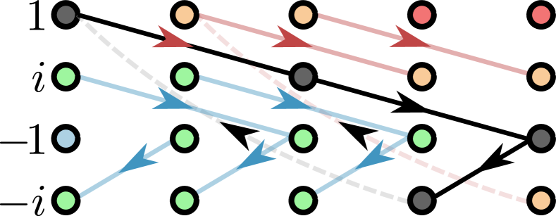
Perhaps the easiest way to understand the relationship between the vector invariant and the boundary behavior is to consider a so-called “sweet spot” model for which the PBC version merely amounts to
| (8) |
where are the winding numbers, and thus the ZTW requirement simply means . In real space, translates to a hopping term of length in the direction. As illustrated in Fig. 3, the ZTW condition implies that when we draw the hopping terms between different sites, it forms closed loops in the bulk, and open chains and isolated sites at the edges.
Computing the chiral charge in a non-Hermitian finite-chain setting is perhaps most straightforwardly done using the formalism of biorthogonal quantum mechanics [26, 27], where we must employ both left and right eigenvectors to compute expectation values. For our purposes, we are interested in the quantity
| (9) |
which counts the total charge of the chiral flavor at the edge labeled by left/right. Here, () contains the right (left) eigenvectors spanning the zero-energy subspace, and and are the projectors to the and edge (the half of the chain containing the edge) subspaces, respectively. In App. C, we show how it is sufficient to treat all sites at the edge that are not part of a complete loop as contributing to the boundary charge.
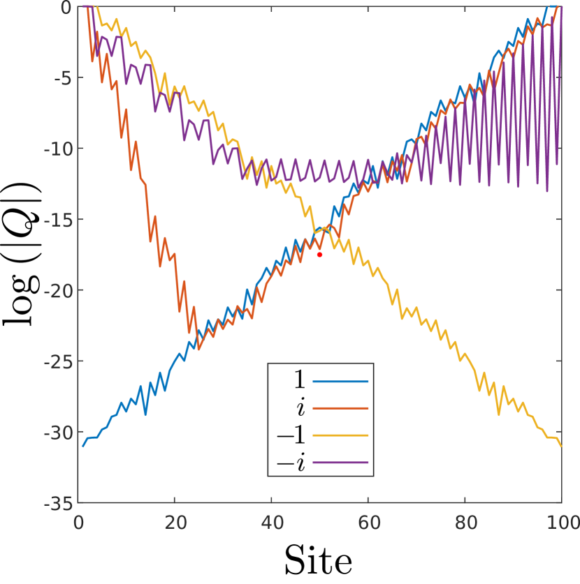
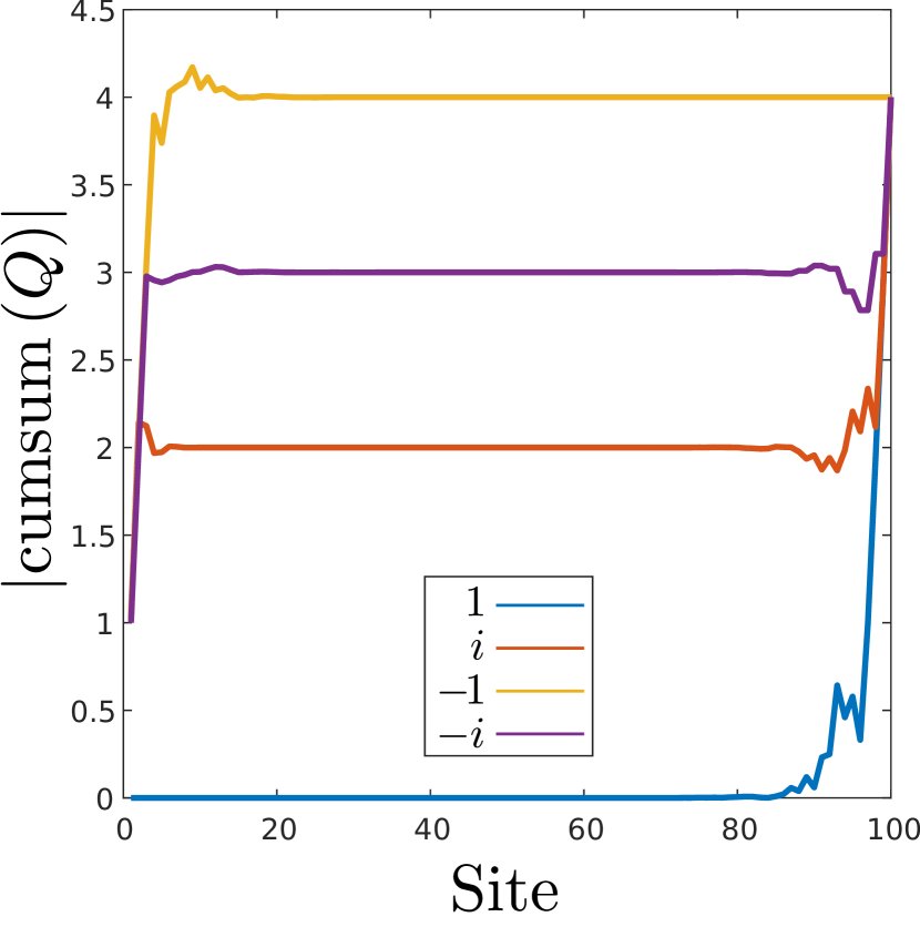
As a concrete example, let us consider a system with – we choose this example as it captures several of the new features not present in conventional chiral systems. Counting sites that are not part of the closed loop in Fig. 3 suggests that , and . Indeed, for a non-sweet-spot model with the same – again constructed in the same way as the models used for Fig. 2 – we can numerically confirm these conclusions; in Fig. 4(a), we show the gapped PBC and OBC spectra for the non-sweet-spot toy model, and in Fig. 4(b) the logarithm of the modulus of the spatial charge distributions for each chiral flavor for the same model. The charge distribution is calculated by replacing in Eq. (9) with a projector to a specific site. Note that this quantity is not real, which is why we only plot the modulus. It only becomes real – or rather the imaginary part becomes exponentially small – once we sum over the sites of half a chain. As we can see from the nearly linear slopes, the charge distributions are exponentially localized to each end. In Fig. 4(c), we calculate the moduli of the cumulative sums and collect them into a vector
| (10) |
for each flavor. Here is the index for the site in question, and is the projector to the th site. This provides a clearer picture of how many charges of each flavor is localized to which edge of the chain.
More generally, the boundary charges (see App. D for the derivation) can be computed from the winding numbers as follows:
-
1.
Define a vector , where the elements are the cumulative sums of the elements of but cyclically permuted so that .
-
2.
.
-
3.
.
The total charge of each flavor is given by , which can be larger than . For and , the inequality is saturated, so that , implying that a strict inequality which can only happen for , marks a clear deviation from the conventional chiral insulator. Indeed, looking back at our example of , we see that there are four of each flavor, which is more than the highest winding .
Given that is a composite number, we can break the symmetry down to a symmetry as we mentioned in the final paragraph of the previous section. In this case, the old chiral flavors combine into the new flavors according to and . In that case, the stable boundary charge would simply be the remaining charge of whichever flavor had the highest charge once we have paired up as many and as possible on a particular edge. For example, on the left edge, we have charges of the new flavor, and of the new flavor. The boundary charge would thus have one charge of the flavor on the left edge (and consequently one charge of the flavor on the right edge) when we take the system to only have symmetry. For a more general discussion on this, see App. E.
Also worth mentioning is that the same set of winding numbers arranged in a different order would yield a completely different charge distribution at the edges; for example, would only have three charges in total for each chiral flavor.
Another novel feature not present in is the non-diagonalizability of the Hamiltonian for certain choices of . Any choice where the corresponding sweet-spot Hamiltonian has broken loops corresponding to Jordan matrices like in Fig. 3 will be non-diagonalizable in the semi-infinite setup. This follows from the observation that the number of left- and right eigenstates for each flavor at each edge is topologically protected by the winding numbers. In App. C, it is also argued that non-diagonalizability does not affect the conclusions regarding the BBC. So in semi-infinite chains, this non-diagonalizability is topologically protected, and suggests that it is not sufficient to look at only eigenvectors when studying topology, but rather the zero-energy subspace which also contains generalized eigenvectors of rank higher than one. However, any finite OBC chain will remain diagonalizable as the states localized at the two edges of the chain will have a finite overlap such that one can always find a proper biorthogonal basis unless fine-tuned to a sweet spot.
V Discussion
In this work, we have studied the topology of systems with a generalized chiral symmetry. The symmetry is an extension of the Bernard-LeClair symmetry classification and can be seen as an additional axis for the periodic table of topological phases labeled by integers . A notable new feature is that the topological phase is specified by a vector of winding numbers rather than a single integer. In one dimension, we saw that the BBC is modified in a non-trivial way such that there now is an unequal number of topological zero-energy states at each chain end, and the largest charge of a given chiral flavor at an edge can exceed the largest winding number in the aforementioned vector. Furthermore, we saw that the topological phase generally corresponds to a non-diagonalizable Hamiltonian in the case of a semi-infinite chain, with the implication that the zero-energy space as a whole rather than only the set of zero-energy eigenvectors is topologically relevant.
The obvious next question theory-wise is what happens in higher dimensions; as seen in App. A, the relation between the overall winding number and the winding number of the subblocks holds true in all odd dimensions, which is highly suggestive of there being related CS phases lurking there. However, the presence/absence of skin modes is no longer merely determined by the overall winding number, but also by weak invariants [23, 22, 24], so extra care needs to be taken. It is also expected that the BBC must be revised, and the nature of the topological modes would most likely no longer be simple Dirac-type cones.
With current technology CS could be implemented in acoustic [28] or photonic systems [29, 30, 31, 17] – indeed, in [17] they realized a gapless version of a CS chain using photonic rings. One could also construct an electric circuits with a Laplacian that mimics the non-Hermitian Hamiltonian through the appropriate combination of electric components [32, 33, 34, 35, 36].
Acknowledgements.
JL acknowledges the support from the National Natural Science Foundation of China under Project 92265201 and the Innovation Program for Quantum Science and Technology under Project 2021ZD0302704.Appendix A Winding Numbers
Even though we are only considering one-dimensional systems in this work, we show here that the total winding number is always a sum of the individual blocks in all odd dimensions. The -dimensional spectral winding number around zero is given by [37, 38]
| (11) |
We observe that the above formula only contains products of the form . Calculating such a product for the Hamiltonian in Eq. (3), gives us
| (12) |
which means that any products of such terms will remain block diagonal, and when we finally perform the trace, it can be achieved by summing the traces of all the individual blocks together.
Appendix B Constructing Non-Island Toy Models
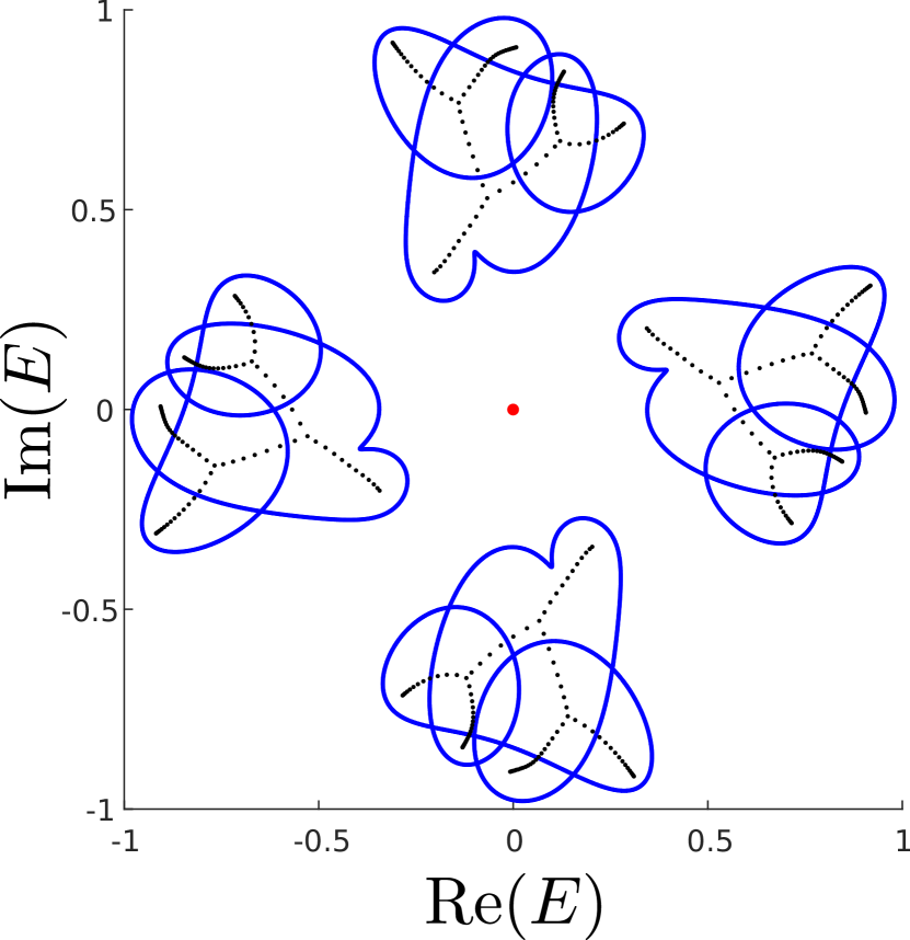
The toy model used in the main text can only give band islands, meaning the spectra will separate into individual bands. This is more directly connected to the conventional Hermitian AIII case, since it consists of two band islands lying on the real line that are mapped to each other via the chiral operator. However, for non-Hermitian systems, this island picture is not a necessary feature, and we can, in fact, also conjure up models where we, for example, have two bands circling the origin but in opposite directions such that the overall winding remains zero. This can be achieved by starting from a block
| (13) |
When the off-diagonal terms are zero, the matrix decouples into two blocks with opposite winding. We can then construct the remaining blocks using for example the template
| (14) |
where the winding is as long as . This can be confirmed by a direct calculation of the winding number using Eq. (5). We provide an illustrative example in Fig. 5, where we have a randomly generated 3-CS model with (with and for the respective two blocks that are not ) where the spectrum wraps around the origin, and the OBC modes are confined to be within the annulus with the two PBC bands as its borders. The sampling is done using the following steps: first we find and in the same way as outlined for and in the main text. Then we define and using a uniformly sampled from . Then we sample the phases from as before. An identical procedure is performed on the diagonal terms. As expected, we still have topological zero modes at the edges.
Appendix C Bulk-Boundary Correspondence
Here we will show that the chiral charge Eq. (9) is preserved at the edge of a semi-infinite chain. In the semi-infinite case, the Hamiltonian is not necessarily diagonalizable, so the zero-energy subspace consists not only of eigenstates, but also of higher-order eigenstates (i.e. eigenstates of powers of the Hamiltonian). To calculate the th chiral charge at time , we must then look at the expression
| (15) |
where
| (16) |
is the projector to the th chiral-charge sector, and and are matrices containing the right and left (including higher order) zero-energy eigenvectors, respectively. Note that they are all eigenvectors of the chiral operator.
We insert between all the terms in the product of Eq. (16). For each term, we get
| (17) |
where is a diagonal matrix containing the eigenvalues of the vectors in with respect to the chiral operator (). We have denoted the Jordan normal form of the zero-energy subspace of the Hamiltonian by . This matrix can be further decomposed into one zero-matrix corresponding to all the one-dimensional Jordan blocks, and another one containing the Jordan blocks of higher dimension. Since , we can treat them independently. For , the exponent reduces to an identity matrix and we straightforwardly obtain the number of chiral charges with flavor in that sector of the zero-energy subspace. For , the story is essentially the same, but we must further note that contains a finite number of terms in its series expansion, but only the zeroth order term – the identity matrix – lies on the diagonal. The rest of the non-zero terms lie above the diagonal. This means that once we multiply all the terms together and take the trace, only the zeroth-order terms survive, so the conclusions are the same as that of . Putting it all together, we get
| (18) |
This means that although higher-order eigenvectors will move away from being chiral eigenvectors, the total charge of any particular flavor is preserved. This may seem paradoxical, but it can be understood by remembering that the higher-order left and right eigenvectors move in “opposite” directions: one evolves into higher chiral flavors corresponding to higher powers of , while the other evolves into lower flavors with their only overlap lying in the original flavor sector.
Appendix D Deriving the Chiral Charge Distribution
To determine the charge of each flavor on a given boundary of the 1-D system, we focus on the sweet-spot case as explained in the main text. To make the discussion clearer, we use the sublattice picture for the different flavors and adjust our language accordingly. The winding number associated with the and sublattices determines the relative position of the site in the th sublattice with respect to the position of a site in the th sublattice to which the former site is connected through the hopping term in the Hamiltonian. For example, site of the th sublattice connects to the site in the th sublattice if . Because the existence of a point gap at zero energy requires the sum of all winding numbers to be zero, and each winding number equals the relative position translation, all such hoppings between sublattices form closed loops in the bulk. The presence of a boundary then cuts some of these loops, leaving behind isolated sites and open chains. These contribute to the boundary charges. Again, keep Fig. 3 in the main text in mind throughout this discussion.
All loops in the bulk have the same shape as determined by the vector invariant in Eq. (7). Consequently, the number of sites not belonging to a complete loop on the left boundary of a given sublattice equals the number of sites to the left of the first site in that sublattice that is a member of a complete loop. In other words, the charge number on the left boundary of that flavor is determined by the relative position of a site in that sublattice with respect to the left-most site of the closest complete loop. For the right edge, we can make analogous statements.
To explicitly determine the left-side boundary charges for a given , we begin by denoting the position of the first flavor in the left-most complete loop by . The positions of the remaining flavors in the loop are then given by a vector of cumulative sums . The left-most position of the loop is then
| (19) |
The left-most position of the left-most loop must coincide with the left boundary, so , or . Then the positions – and hence the total left-boundary charge – of a given flavor is simply given by
| (20) |
where in the last line we have introduced the notation of the main text. For the right charges, we can do a similar analysis, using the maximum instead of the minimum.
Appendix E Boundary Charges when Reducing the Symmetry of Composite
For a CS system with composite , where , we can break the CS symmetry down into a reduced CS. This means that the original chiral flavors are grouped such that we are left with flavors. In this appendix, we will see how to calculate the number of boundary charges for the new flavors in terms of the charges for the old flavors. We will only do the left boundary as the right boundary can be calculated in an analogous way.
We saw that breaking the symmetry into a smaller CS leads to replacing the original vector invariant of length to one of length with the components
| (21) |
We consider only the left boundary, as the right boundary can be done in an analogous way. Following the recipe for calculating the boundary charges as outlined in the main text and derived in App. D, the new vector – denoted here by – is given by
| (22) |
where we have introduced the original CS vector, and then rewritten the difference in terms of the corresponding left-boundary charge vector . The new left-boundary charges are then , or more explicitly:
| (23) |
This implies that the left-boundary charges are simply given by first summing together the charges of all the old flavors that now belong the same new flavor, and then subtracting the smallest of these sums. This can be understood by remembering that we can move away charges from zero energy without breaking the symmetry only if we combine states corresponding to a complete set of flavors. This means that if we have all flavors at a boundary, we can remove as many charges from each flavor as there are complete -tuplets. The number of complete -tuplets equals the smallest charge number among the flavors.
References
- Kunst et al. [2018] F. K. Kunst, E. Edvardsson, J. C. Budich, and E. J. Bergholtz, Biorthogonal bulk-boundary correspondence in non-hermitian systems, Physical review letters 121, 026808 (2018).
- Alvarez et al. [2018] V. M. Alvarez, J. B. Vargas, and L. F. Torres, Non-hermitian robust edge states in one dimension: Anomalous localization and eigenspace condensation at exceptional points, Physical Review B 97, 121401 (2018).
- Xiong [2018] Y. Xiong, Why does bulk boundary correspondence fail in some non-hermitian topological models, Journal of Physics Communications 2, 035043 (2018).
- Yao and Wang [2018] S. Yao and Z. Wang, Edge states and topological invariants of non-hermitian systems, Physical review letters 121, 086803 (2018).
- Bender and Boettcher [1998] C. M. Bender and S. Boettcher, Real spectra in non-hermitian hamiltonians having p t symmetry, Physical review letters 80, 5243 (1998).
- Bender [2007] C. M. Bender, Making sense of non-hermitian hamiltonians, Reports on Progress in Physics 70, 947 (2007).
- Kawabata et al. [2019] K. Kawabata, K. Shiozaki, M. Ueda, and M. Sato, Symmetry and topology in non-hermitian physics, Physical Review X 9, 10.1103/physrevx.9.041015 (2019).
- Esaki et al. [2011] K. Esaki, M. Sato, K. Hasebe, and M. Kohmoto, Edge states and topological phases in non-hermitian systems, Physical Review B 84, 205128 (2011).
- Gong et al. [2018] Z. Gong, Y. Ashida, K. Kawabata, K. Takasan, S. Higashikawa, and M. Ueda, Topological phases of non-hermitian systems, Physical Review X 8, 031079 (2018).
- Leykam et al. [2017] D. Leykam, K. Y. Bliokh, C. Huang, Y. D. Chong, and F. Nori, Edge modes, degeneracies, and topological numbers in non-hermitian systems, Physical review letters 118, 040401 (2017).
- Lieu [2018] S. Lieu, Topological phases in the non-hermitian su-schrieffer-heeger model, Physical Review B 97, 045106 (2018).
- Shen et al. [2018] H. Shen, B. Zhen, and L. Fu, Topological band theory for non-hermitian hamiltonians, Physical review letters 120, 146402 (2018).
- Zhou and Lee [2019] H. Zhou and J. Y. Lee, Periodic table for topological bands with non-hermitian symmetries, Physical Review B 99, 10.1103/physrevb.99.235112 (2019).
- Liu et al. [2019] C.-H. Liu, H. Jiang, and S. Chen, Topological classification of non-hermitian systems with reflection symmetry, Physical Review B 99, 125103 (2019).
- De Nittis and Gomi [2019] G. De Nittis and K. Gomi, On the k-theoretic classification of dynamically stable systems, Reviews in Mathematical Physics 31, 1950003 (2019).
- Marques and Dias [2022] A. M. Marques and R. G. Dias, Generalized lieb’s theorem for noninteracting non-hermitian -partite tight-binding lattices, Physical Review B 106, 10.1103/physrevb.106.205146 (2022).
- Viedma et al. [2023] D. Viedma, A. M. Marques, R. G. Dias, and V. Ahufinger, Topological -root su-schrieffer-heeger model in a non-hermitian photonic ring system (2023), arXiv:2307.16855 [physics.optics] .
- Baxter [1989] R. Baxter, A simple solvable hamiltonian, Physics Letters A 140, 155 (1989).
- Alicea and Fendley [2016] J. Alicea and P. Fendley, Topological phases with parafermions: theory and blueprints, Annual Review of Condensed Matter Physics 7, 119 (2016).
- Ni et al. [2019] X. Ni, M. Weiner, A. Alu, and A. B. Khanikaev, Observation of higher-order topological acoustic states protected by generalized chiral symmetry, Nature materials 18, 113 (2019).
- Li et al. [2021] Y.-Z. Li, Z.-F. Liu, X.-W. Xu, Q.-P. Wu, X.-B. Xiao, M.-R. Liu, L.-L. Chang, and R.-L. Zhang, Zero-energy corner states protected by generalized chiral symmetry in symmetric crystals, New Journal of Physics 23, 043010 (2021).
- Zhang et al. [2020] K. Zhang, Z. Yang, and C. Fang, Correspondence between winding numbers and skin modes in non-hermitian systems, Physical Review Letters 125, 126402 (2020).
- Okuma et al. [2020] N. Okuma, K. Kawabata, K. Shiozaki, and M. Sato, Topological origin of non-hermitian skin effects, Physical review letters 124, 086801 (2020).
- Zhang et al. [2022a] K. Zhang, Z. Yang, and C. Fang, Universal non-hermitian skin effect in two and higher dimensions, Nature Communications 13, 10.1038/s41467-022-30161-6 (2022a).
- [25] The magnitude of the winding corresponds to the number of skin modes, and the sign tells us which side of the chain they will localize on; in general, the left and right eigenstates of a non-hermitian hamiltonian are not “the same”. the winding around the point will tell us how many right skin modes exist for [23, 22]. for the left eigenstates of , the equation they need to satisfy is , i.e. , which means that we must instead look at . the left skin modes will localize on the opposite edge compared to the right skin modes.
- Brody [2013] D. C. Brody, Biorthogonal quantum mechanics, Journal of Physics A: Mathematical and Theoretical 47, 035305 (2013).
- Edvardsson et al. [2023] E. Edvardsson, J. L. K. König, and M. Stålhammar, Biorthogonal renormalization (2023), arXiv:2212.06004 [quant-ph] .
- Zhang et al. [2021] X. Zhang, Y. Tian, J.-H. Jiang, M.-H. Lu, and Y.-F. Chen, Observation of higher-order non-hermitian skin effect, Nature communications 12, 5377 (2021).
- Longhi et al. [2015a] S. Longhi, D. Gatti, and G. Della Valle, Non-hermitian transparency and one-way transport in low-dimensional lattices by an imaginary gauge field, Physical Review B 92, 094204 (2015a).
- Longhi et al. [2015b] S. Longhi, D. Gatti, and G. D. Valle, Robust light transport in non-hermitian photonic lattices, Scientific reports 5, 13376 (2015b).
- Longhi [2018] S. Longhi, Non-hermitian gauged topological laser arrays, Annalen der Physik 530, 1800023 (2018).
- Hofmann et al. [2019] T. Hofmann, T. Helbig, C. H. Lee, M. Greiter, and R. Thomale, Chiral voltage propagation and calibration in a topolectrical chern circuit, Physical review letters 122, 247702 (2019).
- Zhang et al. [2022b] R.-L. Zhang, Q.-P. Wu, M.-R. Liu, X.-B. Xiao, and Z.-F. Liu, Complex–real transformation of eigenenergies and topological edge states in square-root non-hermitian topolectrical circuits, Annalen der Physik 534, 2100497 (2022b).
- Zeng and Lü [2022] Q.-B. Zeng and R. Lü, Evolution of spectral topology in one-dimensional long-range nonreciprocal lattices, Physical Review A 105, 042211 (2022).
- Liu et al. [2021] S. Liu, R. Shao, S. Ma, L. Zhang, O. You, H. Wu, Y. J. Xiang, T. J. Cui, and S. Zhang, Non-hermitian skin effect in a non-hermitian electrical circuit, Research (2021).
- Zou et al. [2021] D. Zou, T. Chen, W. He, J. Bao, C. H. Lee, H. Sun, and X. Zhang, Observation of hybrid higher-order skin-topological effect in non-hermitian topolectrical circuits, Nature Communications 12, 7201 (2021).
- Budich and Trauzettel [2013] J. C. Budich and B. Trauzettel, From the adiabatic theorem of quantum mechanics to topological states of matter, physica status solidi (RRL)–Rapid Research Letters 7, 109 (2013).
- Schnyder et al. [2008] A. P. Schnyder, S. Ryu, A. Furusaki, and A. W. Ludwig, Classification of topological insulators and superconductors in three spatial dimensions, Physical Review B 78, 195125 (2008).