Sagamihara 252-0373, Japan
Analytic Approach for Computation of Topological Number of Integrable Vortex on Torus
Abstract
An analytic method to calculate the vortex number on a torus is constructed, focusing on analytic vortex solutions to the Chern-Simons-Higgs theory, whose governing equation is the so-called Jackiw-Pi equation. The equation is one of the integrable vortex equations and is reduced to Liouville’s equation. The requirement of continuity of the Higgs field strongly restricts the characteristics and the fundamental domain of the vortices. Also considered are the decompactification limits of the vortices on a torus, in which “flux loss” phenomena occasionally occur.
1 Introduction
Vortices are ubiquitous structures in various scales of nature. They typically demonstrate a topologically non-trivial configuration of fields both in quantum and classical dynamics Abrikosov:1956sx ; Nielsen:1973cs ; Manton:2004tk . We define the vortices here as the localised static solutions to a gauge theory coupled with a matter, or a Higgs field. A characteristic example of the vortices is the magnetic flux in type-II superconductors, which appeared as the topological solitons in the Ginzburg-Landau(GL) model, namely, the static energy functional of the 2+1 dimensional Abelian-Higgs model. Those vortices in GL model emerge as the defects of field configuration with a spontaneous phase transition of the system, in which the ordinary Maxwell electromagnetism governs the dynamics of the vortices described by an Abelian gauge field. In 2+1 dimensions or 3 spatial dimensions, another “dynamics” for the gauge fields is possible: one can incorporate the Chern-Simons three-form, which brings topological degrees of freedom. The physical significance of the Chern-Simons term stems from the fact the theory including it serves as an effective theory of the quantum Hall effect Tong:2016kpv ; Klitzing2020 . The vortex solutions may notably exist in the Maxwell-Chern-Simons-matter theories and the pure Chern-Simons-matter theories Horvathy:2008hd . In this paper, we consider the Jackiw-Pi vortex equation, which governs the non-relativistic Chern-Simons-matter theory in the static case, and its vortex solutions.
In ordinary Abelian-Higgs vortices such as in type-II superconductors, the flux of the gauge field, i.e., the magnetic flux, is concentrated at the zeroes of the Higgs field. However, another kind of vortices exists for which the magnetic flux is excluded from the Higgs zero, sometimes referred to as exotic vortices Walton:2021dgi . The Jackiw-Pi vortices belong to the latter case.
As with the ordinary field theories, the field equations governing the vortices are also second-order differential equations. However, situations in which they become first-order equations exist if the coupling constants obey critical relations, i.e., the BPS (Bogomolnyi-Prasad-Sommerfield) limits. In such cases, the system of first-order BPS equations is equivalent to the celebrated Liouville equation, a second-order solvable differential equation. In Manton:2016waw , Manton shows that five distinct cases of such integrable vortex equations exist according to the curvature of the background surfaces on which the vortex lives. Among the five equations, the Taubes equation Taubes:1979tm , the Ambjørn-Olesen equation Ambjorn:1988fx , and the Bradlow equation Bradlow:1990ir are defined on a hyperbolic surface of constant curvature , while the Popov equation Popov:2007ms ; Popov:2008gw is defined on a sphere . The integrable vortex equation on a plane is the Jackiw-Pi equation Jackiw:1990aw ; Jackiw:1990tz considered in the present paper. There exist some geometrical interpretations behind those integrable vortex equations. In Baptista:2012tx , the Higgs fields of the vortices are explained as conformal factors of a metric of the constant curvature surface with isolated singularities. In Contatto:2017alh , it is interpreted that these integrable equations can be reduced from four-dimensional Yang-Mills theories, and the relation between the vortices and a flat non-Abelian connection in three-dimensions is shown in Ross:2021afj . In addition, the higher-order generalizations in terms of the “vortex polynomials” to those integrable vortex equations are considered in Gudnason:2022hxu , which includes the equations from Chern-Simons theories.
Although the integrable vortices except for the Popov vortices are defined on non-compact surfaces, they may also live on compact surfaces of constant curvature, i.e., the surfaces of genus . For those vortices, the periodicity of the background surfaces strongly restricts the solution spaces to the vortex equations. For the cases of , the Jackiw-Pi vortices on a torus are considered earlier in Olesen:1991dg and reconsidered in Akerblom:2009ev , in which the elliptic functions describe the vortices. For the cases of , a special solution to the Taubes equation is constructed with Schwarzian triangular functions Manton:2016waw . However, a comprehensive understanding of the vortices on compact surfaces has not been achieved. For example, a systematic approach to calculating the characteristics of the vortices such as the vortex number is not established. In this paper, we will show an analytical method for determining the vortex number on a torus, namely the first Chern number, and aim to elucidate the vortices on compact surfaces in detail.
Another topic of solitonic objects on compact spaces such as torus is the possibility of having twisted periodic conditions, which leads to the so-called fractionally charged solitons, e.g., Bruckmann:2007zh . Those kinds of objects are one of the key research interests for the physics of confinement tHooft:1981nnx ; Gonzalez-Arroyo:2019wpu ; Anber:2023sjn , however, we do not consider the twisted periodic conditions here and remain them as a subject of future research.
The study of topological objects such as vortices, skyrmions, etc., is actively performed and still underway. Although the integrability of such systems is essential, soliton-like phenomena also appear in the systems without integrability, e.g., Koike:2022gfq . These are important interdisciplinary studies of physics, mathematics, and other areas of science. In particular, these solitonic objects on the spaces with periodicity, which may be interpreted as compact spaces, would provide an important contribution to condensed matter physics as well as mathematical physics. In this context, the possibility of interpreting water waves as topological solitons has been proposed in Smirnova:2023 . This direction would open a new window into the research for topological solitons. It is important to clarify the meaning of integrability in nature.
This paper is organized as follows. In the next section, we define the model deriving the Jackiw-Pi equation and give an outline of the integrable vortex equations. In section 3, we construct a method for the analytic calculation of the vortex number on compact surfaces and analyse typical cases with specific examples. In section 4, the decompactification limits of the vortex solutions are considered on a torus. In the final section, we give conclusions and discussions.
2 The Jackiw-Pi equation
In this section, we inaugurate the Jackiw-Pi vortex equation from some field theoretical point of view. We firstly introduce the integrable vortex equations on constant curvature surfaces discussed by Manton Manton:2016waw and see the Jackiw-Pi equation is one of the five integrable equations derived from the Abelian Higgs model. As an alternative derivation of the Jackiw-Pi equation, we also focus on the non-relativistic Chern-Simons-matter theory. We then give the general solutions to the Jackiw-Pi equation in terms of a meromorphic function on a flat plane and a torus .
2.1 Integrable vortices
We consider a complex scalar field with a quartic potential coupled with an abelian gauge field on a two-dimensional surface with critical coupling constants Manton:2004tk . Let be a surface with conformal metric , where the conformal factor is a function of and . The static energy functional of such the Abelian Higgs model on is
| (2.1) |
where , is the field strength, and are the covariant derivatives with respect to gauge potentials and , and is a complex Higgs field. The real constants and will be specified later. Applying the Bogomolny completion to this energy functional, we obtain the following formula,
| (2.2) |
where
| (2.3) |
is the first Chern number taking an integer value. The integer (2.3) is interpreted as the number of the vortices considering with multiplicity and is a topological invariant because it is independent of the metric of . From this formula, if the following Bogomolny equations,
| (2.4) |
are satisfied, we find the energy is bounded below if , thus the field configurations satisfying (2.4) are stable. However, we will discuss the case of below and in the next section from another point of view. Eliminating by using the first equation of (2.4), we obtain the following equation,
| (2.5) |
where we have defined and . We refer to the equation (2.5) as the generalised vortex equation.
We note that the values of the constants and can be normalised as either or by rescaling the metric and . In ref.Manton:2016waw , Manton argued that there are nine possible ways to choose and , but the four cases of them are invalid: The right-hand-side of (2.5) must be positive since the left-hand side of (2.5) is the magnetic field whose integral gives the positive topological number . Therefore the remaining five cases are acceptable.
There is a geometrical interpretation of the constants and in the generalized vortex equations Baptista:2012tx . Let , where is the metric of . The new metric obtained by conformally rescaling the original metric with the squared Higgs field is referred to as the Baptista metric Baptista:2012tx . Let the Gaussian curvatures of the original metric and that of the Baptista metric , respectively. We find
| (2.6) |
where is the Euclidean Laplace operator. From (2.6), the relation between the two curvatures is
| (2.7) |
Because is a solution to the generalized vortex equation (2.5), we obtain the following relation
| (2.8) |
by using (2.5).
The relation (2.8) is crucial for the integrability of the generalised vortex equation. Let us consider the curvature is equal to the constant , then equals from (2.8). If this is the case, as the curvature , the differential equation providing (the latter of (2.6)) can be written as
| (2.9) |
where . This equation, or the equation with new variable
| (2.10) |
is called Liouville’s equation, which is one of typical integrable equations. It is known that the general solution to Liouville’s equation is
| (2.11) |
where and are arbitrary holomorphic functions of and defined on the original surface , respectively. Hereafter, we restrict ourselves that the case , namely,
| (2.12) |
for the geometrical interpretation of vortices. Now we consider the case that is a constant curvature surface, i.e., is a constant. Then we find the metric of takes the form
| (2.13) |
Recalling that , we obtain a representation of in terms of ,
| (2.14) |
From (2.14), we find that the squared Higgs field can be considered as the quotient of a metric of constant curvature surface with complex coordinates and ,
| (2.15) |
and that of . Hence, the zeroes of the Higgs field, where the vortex centres are sitting, are the indefinite points of the surface . This means that is a constant curvature surface with orbifold-like singularities at the vortex centres.
We introduce the Jackiw-Pi equation as a special case of the generalized vortex equations (2.5). The Jackiw-Pi equation is the integrable vortex equation defined on a flat Euclidean plane, i.e., the background curvature and the conformal factor . From Manton’s classification, the case of is the only possible case. Then the target surface is , and the Jackiw-Pi equation takes the form
| (2.16) |
This is also Liouville’s equation. The solution to Liouville’s, or the Jackiw-Pi equation is therefore,
| (2.17) |
or
| (2.18) |
where is a meromorphic function on . The meromorphicity of is required by the target surface being .
2.2 Non-relativistic Chern-Simons-matter theory and the Jackiw-Pi equation
As we already mentioned, the Jackiw-Pi equation can be derived from another point of view. In this subsection, we review that the equation is the governing equation to the dimensional non-relativistic Chern-Simons-matter theory for its static and (anti-)self-dual solutions. The vortex solutions to the Jackiw-Pi equation are unstable from the perspective of the Abelian-Higgs model, since the positiveness of , as seen above. We can avoid this instability of the vortices in the Chern-Simons-matter theory.
We introduce the following Lagrangian density,
| (2.19) |
where is a complex scalar field, is the covariant derivative with an Abelian gauge field , , and is the field strength. The metric and the complete anti-symmetric tensor are defined as and , respectively. The Euler-Lagrange equations to this system are
| (2.20) | ||||
| (2.21) |
where with
| (2.22) | ||||
| (2.23) |
The field equations (2.21) are decomposed as
| (2.24) | ||||
| (2.25) |
where and are understood.
Making use of an identity
| (2.26) |
where , we can rearrange (2.20) into
| (2.27) |
We now consider the static solutions to (2.27) with , then (2.27) is reduced to be
| (2.28) |
Taking a gauge
| (2.29) |
(2.28) becomes
| (2.30) |
This can be solved by the following “self-dual” or ”anti-self-dual” ansatz
| (2.31) | |||
| (2.32) |
the latter is referred to as the (anti-)self-dual coupling. The defining equation for the scalar fields (2.31) is first order in its derivatives, so we refer to it as the BPS equation. From the BPS equation (2.31) with (2.24), we obtain the Jackiw-Pi equation again,
| (2.33) |
where we have chosen and . Thus we find that the magnetic flux density is proportional to the scalar field density
| (2.34) |
from (2.24) in contrast to the ordinary GL theory.
The static energy with these ansatz turns out to be
| (2.35) |
thus the energy takes minimum value for the (anti-)self-dual solutions. Hence the BPS vortex solutions to the non-relativistic Chern-Simons matter theory (2.19) can be regarded as stable configurations.
Hereafter we unify the expression of the scalar field with and refer to it as the Higgs field, and consider the Lagrangian (2.19) governs the dynamics of the system.
2.3 Vortex solutions on torus
As shown above, the Jackiw-Pi equation is equivalent to Liouville’s equation so that arbitrary holomorphic functions give the local solutions. For the solutions to be regular vortices, we should pay attention to the global behaviour of the field configurations: the finiteness of the flux, or energy, should be imposed. This requirement certainly gives restrictions for the holomorphic functions.
Firstly, we consider the vortex solutions defined on a flat plane . It has been shown that the Higgs field given in (2.17) yields the Jackiw-Pi vortices on if, and only if, the meromorphic function takes the form
| (2.36) |
where and are polynomials such that Horvathy:1998pe ; Akerblom:2009ev . In this case, the vortex number of the solution is proved to be .
Next, we focus on the vortices on a torus . In this case, it is sufficient to impose the doubly periodicity for the Higgs field to be regular vortices. It is obvious that imposing the doubly periodicity for the meromorphic functions leads to that of the Higgs field. The well-known fact is that the general doubly periodic functions are given in terms of the Weirestrass elliptic function and its derivative on a periodic lattice , where and are independent complex numbers with positive imaginary part, so-called the half-periods, e.g., whittaker_watson_1996 . The corresponding doubly periodic meromorphic functions are
| (2.37) |
where and are some rational functions. Although the general form of the meromorphic function , or the Higgs field, is given, the characteristic quantities of vortices such as the vortex number are not obvious from (2.37). As shown in the next section, we consider the concrete examples for to analyse the structure of individual vortices in detail.
We point out here that the Higgs field itself would not be an observable quantity of the theory but it would be the flux density . If this is the case the Higgs field itself is not necessary to be doubly periodic: it only needs quasi-doubly periodicity concerning the lattice , i.e.,
| (2.38) |
where are some phase angles. In this context, Akerblom et.al. Akerblom:2009ev found the general doubly periodic solutions for the flux density . From the gauge theoretical perspective, the quasi-periodic field configurations are admittable because the fields are periodic up to gauge transformation in those cases. However, we consider in this paper the Jackiw-Pi vortices on constructed from the strict doubly periodic Higgs field itself. The reason is that the continuity of the Higgs field as a complex function is necessary for the analytic calculation of the vortex number, which takes integer values. On the other hand, the quasi-periodic Higgs fields would give rise to the solitonic objects with non-trivial holonomy. For that kind of vortices, the vortex numbers would be able to take fractional values just as in the case of fractional instantons tHooft:1981nnx ; vanBaal:1982ag ; Gonzalez-Arroyo:2019wpu . Although these are interesting solitonic objects, we concentrate here on the trivial holonomy vortices based on the Higgs fields with strict doubly periodicity.
3 Analytic calculation of vortex number on torus
In this section, we establish the analytic calculation method for the vortex number of the Jackiw-Pi vortices on a torus. The crux of the method is reconsidering the integral (2.3) that determines the vortex number: representing it in an expansion of the Higgs field around its zeroes, i.e., the vortex centres. Then we apply the method to several examples including the vortices with simple zero and also multiple zero. Here we give the details of the approach. An outline of the procedure has been reported in Miyamoto:2023qwe 111The contents of this report include inaccuracies. by the present authors.
3.1 Strategy for analysis
Let us recall that the vortex number of the Jackiw-Pi vortices on 2-dimensional space is given by the first Chern number,
| (3.1) |
We notice that if is a closed surface such as a torus, this integral seems to vanish as the surface has no boundary due to the Stokes theorem:
| (3.2) |
However, numerical integration suggests that does not vanish even if is a torus, and the value of takes a certain integer value.
The principal bundle argument has solved this contradiction Akerblom:2009ev , in which the connection form of the bundle is not defined globally on a compact base space such as that of Dirac monopoles. In such cases, the transition functions of the bundle carry all of the information for the field configurations. Thus we can find the vortex number takes an integer value from the argument. Nevertheless, we face the difficulty: although the vector bundle argument shows us that is an integer, it does not give the value concretely. However, as mentioned above, we can obtain the vortex number explicitly with numerical integration. We expect that the vortex number on a torus is supposed to be the sum of the multiplicity of Higgs zeroes, or the winding number, as an analogy to the case of vortices on a flat plane. The analytical method constructed in this section will provide the vortex number exactly and prove this expectation.
We begin with reconsidering the background surface, i.e., the torus, on which the flux is defined. Let be a solution to the Jackiw-Pi equation possessing zeroes at . We have to pay attention that the Liouville equation (2.16) or (2.33) is not defined at the zeroes of , the vortex centre, due to the logarithmic singularities of the equation. It suggests that we should define the natural domain of as the torus without singular points:
| (3.3) |
The boundaries of are infinitesimal circles around zeroes of . Then the integral (3.1) turns out to be
| (3.4) |
through Green’s theorem and it may not vanish, where the integration contours rotate counterclockwise. The derivation to (3.4) is given in Appendix A.
We now evaluate the contour integral (3.4) around the zeroes of . We notice from (2.17) that the zeroes of may arise from the zeroes of or the poles of . Firstly, let us consider the former cases in which the meromorphic function has a simple zero at, say . In such cases, can be expanded into the form of Taylor expansion around as
| (3.5) |
where ’s are complex coefficients. Thus one can expand around as
| (3.6) |
where and is the terms of order and higher in and their products. Evaluating -derivative part of the integrand of (3.4) around simple zero , we find
| (3.7) |
On the small circle around , we take the parametrisations , and , where . Taking the limit with these parametrisations, we observe
| (3.8) |
Similarly, the -derivative part becomes
| (3.9) |
where is applied. Therefore the integrand of the right-hand-side of (3.4) turns out to be
| (3.10) |
on the small circle around a simple zero . By integrating it, we obtain a unit vortex number for each simple zero. Hence, the contribution to the vortex number from the simple zeroes of is
| (3.11) |
where ’s are the location of simple zeroes.
We next consider the Higgs zeroes emerging from the zeroes of with order . In such cases, the meromorphic function has the expansion around the order zero
| (3.12) |
Similarly to the simple zero cases, the Higgs field is expanded around as
| (3.13) |
where is a complex constant composed of the expansion coefficients of and is the terms of order and higher in , and their products as in the simple zero case. Thus we find
| (3.14) |
and
| (3.15) |
where the parametrization around is similar to the simple zero case. From this expansion, the contribution to the vortex number from order zeroes is (3.4)
| (3.16) |
Hence the Higgs zero of order emerged from the -th zero of contributes to the vortex number from (3.4).
Finally, we consider the Higgs zeroes that emerged from the poles of the meromorphic function . Assuming that has an order pole at with , the Laurent expansion of around is
| (3.17) |
then its derivative is
| (3.18) |
where is a complex coefficient and is the terms of order and higher in . Note that the singularities of are only poles since it is meromorphic. To find the behaviour of the Higgs zeroes, we observe that
| (3.19) |
where is the terms of order and higher in , and their products. Note that the terms may include negative powers of and such as in contrast to the former cases. Thus the behaviour of the Higgs field around is
| (3.20) |
and similarly,
| (3.21) |
We find from (3.1) that the zeroes of the Higgs field emerge from the cases , while the case gives a non-zero point. The contour integral around for the case does not contribute to the vortex number and the point becomes a saddle point of because there remains no radius dependence in its leading order at this point, as we will see later in some examples. We thus observe that
| (3.22) |
and
| (3.23) |
around , respectively. The -derivative part of the contour integral of (3.4) and its -derivative counterpart for these cases become
| (3.24) |
and
| (3.25) |
respectively, where the parametrization etc., is applied as in the former cases. Note that the term such as does not contribute to the contour integral around because it has order . Hence the contour integral is evaluated as in the previous cases
| (3.26) |
Therefore, we find that the Higgs zero emerged from the order poles of contributes to the vortex number . We note that the order poles of do not contribute to the vortex number since they do not give the zero points of , namely, not the vortex centres.
To summarize this subsection, we have proposed an analytical method to calculate the vortex number of the Jackiw-Pi vortex on a torus. In this approach, the defining region of the flux is regarded as a torus without the singular points corresponding to the centres of the vortex, namely, the Higgs zeroes. The evaluation of the flux integration is given through the expansion around each singular point and contour integration. It is shown that there are two types of Higgs zeroes: One of them arises from the zeroes of the derivative of a meromorphic function , and the other emerges from the poles of . The contribution to the vortex number is from the order zeroes of , and from the order poles of .
3.2 Vortices from elliptic functions: Examples
Let us examine typical examples of the Jackiw-Pi vortices on a torus. We choose simple elliptic functions as a meromorphic function and see the characteristic aspects of the Higgs fields for individual vortices. In particular, we perform analytic calculations for the vortex number developed in the previous subsection and see the consistency with the numerical integration. It is well known that there are two kinds of fundamental doubly periodic functions, namely, the Weierstrass function and the Jacobi elliptic function. We will find that the characteristic difference appears between the vortices constructed from these fundamental elliptic functions.
Example 1: Weierstrass function
First of all, let us consider simply the Weierstrass function for the meromorphic function , then the Higgs field becomes
| (3.27) |
where are the half-periods of the lattice 222In some literatures these are defined as the whole-periods. , and is doubly periodic with respect to the lattice. The -function enjoys the differential equation
| (3.28) |
where and are constants and the dependence of the and is omitted. The values of -function at its half-periods are denoted as with , and there exist relations , and . It is known that the function has a double pole at the origin such as
| (3.29) |
Hence the Higgs field has a zero with a unit vortex number at the origin from the discussion of the previous subsection. We find from (3.1) that the phase angle rotates three times around the origin,
| (3.30) |
where and are employed.
On the other hand, the has simple zeroes at the half-period points and , so that there exist three simple zeroes of the Higgs field at that points. We observe that the phase angle rotates once around these simple zeroes,
| (3.31) |
from (3.6), where with and . Thus we find these zeroes, namely the vortex centres, contribute to the vortex number from (3.11) so that the total vortex number of this solution is . This is consistent with the numerical integration for the first Chern number (3.1) performed with Mathematica,
| (3.32) |
where (2.34) is applied.
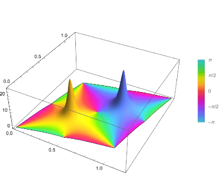
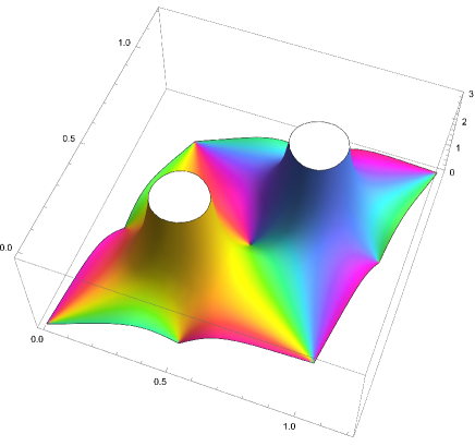
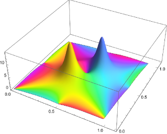
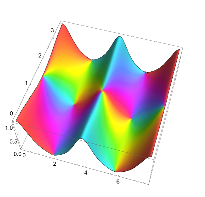
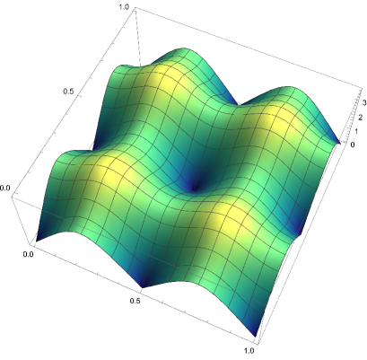
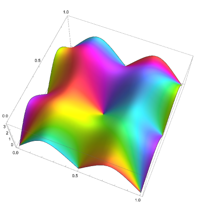
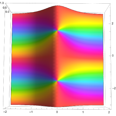
Figure 1 shows the profile of the Higgs field with half-periods and . The four zero points exist at and in the fundamental lattice. The phase angle structure shows the three times rotation around , while the rotations are once around the other zeroes at , as expected.
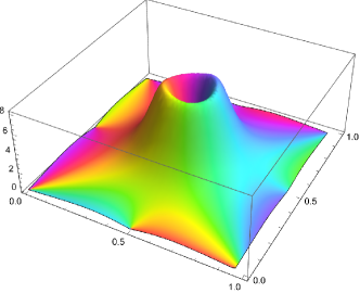
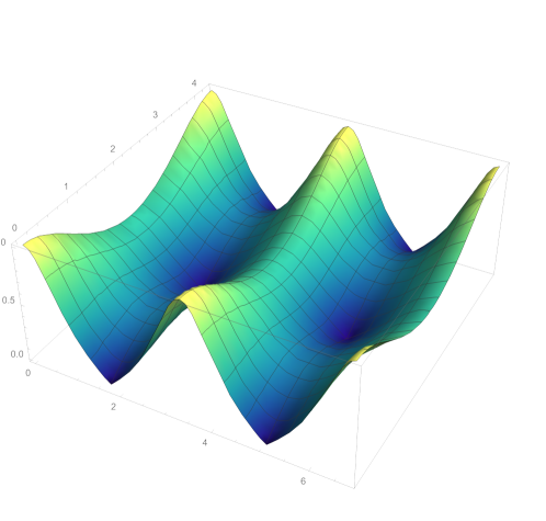
The absolute value of the Higgs field indicates that the flux is localised at the twin peaks on the fundamental lattice. This localisation structure is not the common feature of but depends on the choice of half-periods as illustrated in Figure 2. As the region of the fundamental lattice tends to be rectangular, the twin peaks eventually merge into a “volcano-like” structure surrounding the zero at .
Example 2: Jacobi sn function
The other fundamental elliptic function is the Jacobi elliptic function. Now we apply the Jacobi function simply as the meromorphic function , then the Higgs field takes the form
| (3.33) |
where and is the modulus. The fundamental lattice on which the function defined is , where and are the complete elliptic integrals of first kind with . We take the modulus as usual, for which so that the fundamental lattice is rectangular.
This vortex solution has four simple zeroes emerging from the simple zeroes of the numerator in (3.33), i.e., and are the zeroes of , and and are those of . In contrast to the -function case, the -function in the denominator has only simple poles at and so they do not give zero points but saddle points from (3.1).
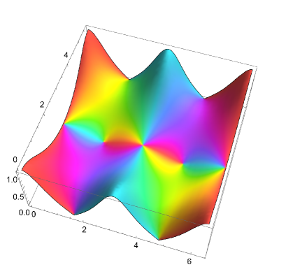
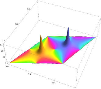
The profiles of with various values of are shown in Figure 3. The four simple zeroes appear, for which the phase angle rotates once around them as expected from (3.6). On the other hand, the phase angle rotates twice around the two saddle points, which is consistent with (3.1) with , namely, the behaviour is
| (3.34) |
The vortex number of these solutions is also four because all four zeroes are simple, which agrees with the numerical integration as with the previous example.
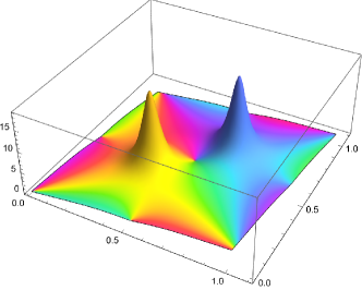
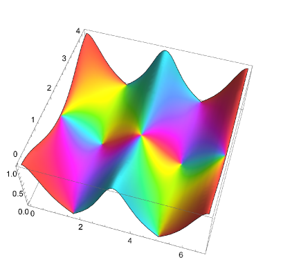
We note that if the phase factor of the Higgs field is ignored the fundamental domain of the solution would be halved in the real axis as shown in Figure 4. This can be understood by the periodicity of the Jacobi elliptic functions , and from (3.33). However, the continuity of the Higgs field as a function of and is lost on this half-domain, on which the phase angle is not periodic at the boundaries so that the formula for the vortex number (3.4) will be invalid. Therefore, we require the strict doubly periodicity of the Higgs field itself in our analysis for the vortices. We will comment on this issue again in the final example.
Example 3: Powers of Jacobi sn function
For a vortex solution with multiple zeroes, we consider a solution constructed from the multiple powers of the Jacobi sn function. As an illustration, we choose as the meromorphic function , the Higgs field takes the form
| (3.35) |
whose fundamental lattice is the same as in the previous example. There are three types of Higgs zeroes in this case: the simple zeroes from and and the double zeroes from in the numerator, and the triple zeroes from the poles of in the denominator. The positions of simple zeroes are and of which the first two are from and the others are from . The double zeroes from are located at and , and the triple zeroes emerging from the poles of are at and . We observe that the vortex number of this solution is , namely, the four simple zeroes, the two double zeroes, and the two triple poles contribute to , , and , respectively. This is consistent with the result of numerical integration.
We remark that the zeroes of the Higgs field can also be identified with rewriting it in terms of elliptic theta functions as,
| (3.36) |
where the variable . Note that the absolute values of the elliptic theta functions do not diverge, we find the zeroes of only come from the zeroes of the theta functions in the numerator. Let , then the simple zeroes of elliptic theta functions and are located at and , respectively. Together with the quasi-periodicity of the elliptic theta functions, and , the zeroes of the Higgs field with accurate multiplicities are found in the fundamental lattice.
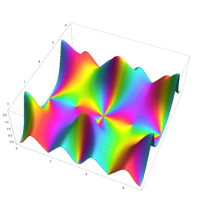
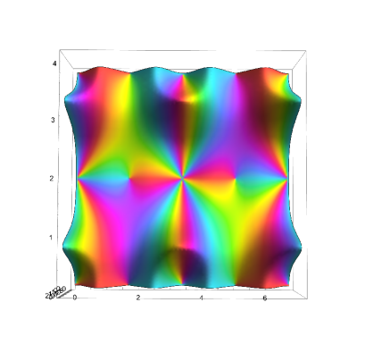
Figure 5 shows the profile of this solution with the phase angle dependence. The simple zeroes are located at and with phase angle rotation . The double zeroes from the numerator at and show the phase angle rotation twice, i.e., as expected from (3.13) with , whereas those from the poles of the denominator at and demonstrate the rotation angle as expected from (3.1) with .
Example 4: Concerning Olesen’s solution
In the early 1990s, Olesen constructed a Jackiw-Pi vortex on a torus with unit vortex number Olesen:1991dg in the context of the Chern-Simons-Higgs theory discussed in the previous section. The meromorphic function defining the solution is
| (3.37) |
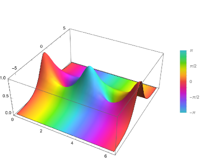
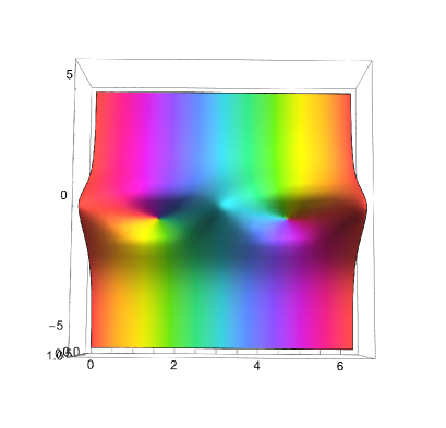
Although the solution is similar to the first example (3.27), a constant shift and an overall scaling are assembled for . This adjustment makes the periodicity of the flux density , or , a quarter of the fundamental lattice region of the function, i.e., . For instance, we show a profile of Olesen’s solution for the square fundamental region for which and in Figure 6.
We find the quarter periodicity in the absolute value of the Higgs field or the flux density, and the quarter region having only one zero. Therefore the vortex number of Olesen’s solution is one from the perspective of the flux density. The general form of the Jackiw-Pi vortices whose flux density has a periodicity of a quarter of the fundamental region of the associated elliptic functions is given in Akerblom:2009ev . This interpretation is reasonable because the physically observable quantity is the flux density and the phase angle of the Higgs field is not significant. However, we find from the right of Figure 6 that the phase angle of the Higgs field is not periodic in the quarter region, so it is not a continuous function in this restricted cell. The continuity of the Higgs field itself is critical for the analytic calculation of the vortex number developed in this paper, so we advocate here the interpretation that the periodicity of this solution is identical to that of the function and the vortex number is since it has four zeroes as of the first example. This interpretation will be acceptable from the point of view of the Aharonov-Bohm-like effects, in which the phase angle of the field plays a critical role.
4 Large period limits of vortices
If we take a fundamental period of the elliptic functions to be infinite, the fundamental lattice expands in that direction and the torus turns out to be a cylinder. Furthermore, the fundamental lattice becomes planar if both of the periods are set to be infinite. In this section, we consider the vortex solutions defined on such large period limits of the fundamental lattice. We will find characteristic “flux loss” phenomena of vortices in those limiting cases.
4.1 Cylinder limits of the vortex from Jacobi elliptic function
To consider the cylinder limit, the vortex made from the Jacobi elliptic functions is favourable because they become elementary functions in the limits.
We reconsider the second example in the last section, i.e., the case of with a modulus . The cylinder limits are obtained by taking the limit or , for which or , respectively. Here we consider the profiles of the Higgs field in these limits and calculate the vortex number of such cases. Then we confirm that they are consistent with numerical integration.
Firstly, we consider the trigonometric function limit . The Higgs field then becomes
| (4.1) |
which has simple zeroes at with . The fundamental region of has an infinite period in the imaginary direction and a period in the real direction, as shown in Figure 7. As a result, the point at infinity is excluded from the fundamental region, in other words, the region becomes open and can be thought of as a cylinder. We parametrise the fundamental region of with as and , for which the simple zeroes of are located at and .
The numerical integration for the vortex number in this cylinder limit is as in the case of a general value of . We now derive this vortex number analytically through (3.4), in that the integration along boundaries at infinity contributes to the vortex number. We evaluate the contour integral
| (4.2) |
where is the cylinder with the Higgs zeroes removed as in the case of the torus. The difference from the torus cases is that the boundary includes the edges at the infinities in its imaginary coordinate. Thus, the contour integral in the right-hand-side of (4.2) is composed of the small circles around the two Higgs zeroes and the two edges at infinities. Since the two zeroes at and are simple, the integration around these zeroes contributes to 2 from (3.6), so that it can be expected that the rest comes from the integration along the edges . We observe the integrands of (4.2) are
| (4.3) |
and
| (4.4) |
The limits of are complex conjugates of (4.4). Hence, can be calculated as follows.
| (4.5) |
Here the orientation of the integral at the edges is set to ensure that the circle rotates counterclockwise around zeroes at infinities, and we should interpret that the Higgs zeroes sent away to infinity still contribute to the integration. This is consistent with numerical integration as mentioned above.
We consider next the hyperbolic function limit , for which turns into . Then the Higgs field becomes
| (4.6) |
In contrast to the former case, the fundamental region of this function has an infinite period in the real direction and a period in the imaginary directions, as shown in Figure 8. Hence the fundamental region is also considered as a cylinder. We take the parametrisation of the fundamental region as and .
The numerical integration for the vortex number in this limit is , in contrast to the trigonometric function case. In the fundamental region, has no zeroes, thus the contribution to the vortex number of will come from the integration on the edges of the region. We now give the analytic calculation for this integration similarly to the former.
The vortex number is also given by (3.4),
| (4.7) |
where are only the edges of the cylinder in this case. The integrands take the following form
| (4.8) |
thus, at the edges ,
| (4.9) |
Hence, can be evaluated as,
| (4.10) |
We should interpret here that the two of four Higgs zeroes fled away from the integration in contrast to the former case. This is also consistent with the numerical integration and illustrates the flux loss phenomena.
4.2 Planar limit
In the examples of the cylinder limit considered so far, the vortex number is not conserved in the limit , while it remains in the limit . We note that a similar flux loss phenomenon has been reported in Akerblom:2009ev , where the authors constructed the vortex on a torus from the elliptic function
| (4.11) |
Here is the Weierstrass function defined on the fundamental latice . They have taken the planar limit of the lattice, for which the function (4.11) tends to , and shown that the vortex number in this limit equals half of that of the torus. Although the meromorphic function does not give a Higgs zero from (3.1) as in the last example, this case also has a vortex number since the integration contour can be taken around infinity in the planar limit.
Here we illustrate another simple case of a vortex in the planar limit. Let us consider the first example of the last section , which leads to a vortex of the vortex number on a torus. If we let both periods be infinite, then the Weierstrass function becomes a rational function, i.e., defined on a plane. On first inspection, this vortex gives the vortex number because the meromorphic function has only a double pole at the origin from the point of view of (3.1). However, it is known that the meromorphic functions give radially symmetric vortices of the vortex number Horvathy:1998pe so that the vortex number will be in this case. We can confirm that no flux loss is observed by evaluating the flux integral as follows. The Higgs field in the planar limit becomes from (4.11)
| (4.12) |
which is rewritten in the polar coordinates
| (4.13) |
where and . The vortex number, or the flux integral, is easily calculated as
| (4.14) |
which indicates no flux loss in the planar limit of the vortex. This observation shows that some relics of the vortex on a torus survive at infinity after taking the planar limit from the perspective of the plane as a decompactified torus. The scenario would be similar to the cylinder limit of a torus considered in the last subsection.
As we have seen in this section, the vortices on a torus occasionally give rise to the flux loss phenomena at the large period limits. We have confirmed this fact in some cases through an analytic manner.
5 Conclusion and discussions
In this paper, we have considered the aspects of the Jackiw-Pi vortices on a torus and, in particular, developed an analytical calculation method to determine the vortex number. The Jackiw-Pi equation can be derived from the Abelian Higgs model on with critical coupling constants, which is also one of the integrable vortex equations proposed by Manton:2016waw . The equation can also be regarded as the “(anti-)self-dual” equation to the Chern-Simons-Higgs theory in dimensions. A meromorphic function characterizes the vortex solution to the Jackiw-Pi equation, and the first Chern number of the gauge field is interpreted as the vortex number. If one chooses an elliptic function as the meromorphic function then the Jackiw-Pi vortex can be thought of as defined on a torus. To determine analytically the value of the vortex number, we propose a calculation method using the expansion of the Higgs field around its zeroes. We advocate that the continuity of the Higgs fields is crucially important for determining the vortex number on a torus. The continuity strongly restricts the fundamental domain of the vortices, as shown in this paper.
In the case of a vortex on a plane, the vortex number is equivalent to the degree of mapping, namely the order of zeroes Horvathy:1998pe , but whether such interpretation applies to the vortex on a torus has not been clear. In this paper, we have shown that the vortex number is given as the sum of the degree of zeroes just as in the planar case even on a torus through the analytical calculation method. It will provide a general procedure for computing the vortex number on a compact surface.
We have also examined some concrete examples of the vortex on a torus and its cylinder or planar limits. Here we discuss the facet of the vortices with the “flux loss” at such decompactification limits. An elliptic function determines a certain elliptic curve, i.e., an algebraic curve of third or fourth order. For example, the Weierstrass -function parametrizes the third order elliptic curve , where and . In the planar limit of the torus considered in the last section, the -function degenerates into the rational function . This means that the elliptic curve degenerates into the third-order curve , which is singular at the origin. The situation is similar to the flux loss case , which degenerates into and the degenerate curve is . The difference between them is that the latter is reducible or factorizable, namely, , while the former is irreducible. Similarly, the cylinder limits of the vortex from the Jacobi elliptic function cases share this characteristic. The meromorphic function parametrizes the fourth order elliptic curve , where and . The trigonometric function limit reduces the curve into a quadratic curve , while the hyperbolic function limit does into . The latter is reducible to . From the discussion in the last section, we notice the trigonometric function limit does not induce the flux loss, while the hyperbolic function limit induces it. As can be inferred from these observations of the decompactification limits, a conjecture might be possible that the flux loss phenomena occur if the corresponding algebraic curve is factorizable into lower-order curves. Whether this conjecture holds or is rejected, we expect that further study unvails the true mechanism of the flux loss.
Finally, we comment on the solutions with twisted periodic conditions mentioned in the Introduction. The vortex solutions considered in this paper have strict periodicity so the vortex numbers are integers. However, there could be the vortices on a torus with twisted periodicity, which have fractional vortex numbers as in the cases of the fractional instantons vanBaal:1982ag ; Bruckmann:2007zh ; Gonzalez-Arroyo:2019wpu . We consider such fascinating objects a subject of future research.
Acknowledgement
K M was supported by the Sasakawa Scientific Research Grant from The Japan Science Society. A N was supported in part by JSPS KAKENHI Grant Number JP 23K02794.
Appendix A Derivation of the formula (3.4)
In this Appendix, we derive the key formula (3.4) for the analysis developed in this paper. We rewrite the field strength in terms of the Higgs field , satisfying the Jackiw-Pi equation. Firstly, we solve the gauge field from ,
| (A.1) |
Similarly, is given by the complex conjugate of (A.1). Hence can be expressed as
| (A.2) |
The surface integration of the field strength on the punctured torus where the Jackiw-Pi vortices are defined then becomes
| (A.3) |
where in the third equality we applied Green’s theorem, e.g., Ablowitz_Fokas_2003 . Here denotes the boundaries of , which are infinitesimal circles around the punctures . We determine the orientation of the circle so that they rotate counterclockwise as shown in Figure 9. We accentuate that the continuity of the Higgs field is critical and necessary in the derivation of (A) for applying Green’s theorem.
References
- (1) A.A. Abrikosov, On the Magnetic properties of superconductors of the second group, Sov. Phys. JETP 5 (1957) 1174.
- (2) H.B. Nielsen and P. Olesen, Vortex Line Models for Dual Strings, Nucl. Phys. B 61 (1973) 45.
- (3) N.S. Manton and P. Sutcliffe, Topological solitons, Cambridge Monographs on Mathematical Physics, Cambridge University Press (2004), 10.1017/CBO9780511617034.
- (4) D. Tong, Lectures on the Quantum Hall Effect, 6, 2016, https://www.damtp.cam.ac.uk/user/tong/qhe.html [1606.06687].
- (5) K. von Klitzing, T. Chakraborty, P. Kim, V. Madhavan, X. Dai, J. McIver et al., 40 years of the quantum hall effect, Nature Reviews Physics 2 (2020) 397.
- (6) P.A. Horvathy and P. Zhang, Vortices in (abelian) Chern-Simons gauge theory, Phys. Rept. 481 (2009) 83 [0811.2094].
- (7) E. Walton, Exotic vortices and twisted holomorphic maps, 2108.00315.
- (8) N.S. Manton, Five Vortex Equations, J. Phys. A 50 (2017) 125403 [1612.06710].
- (9) C.H. Taubes, Arbitrary N: Vortex Solutions to the First Order Landau-Ginzburg Equations, Commun. Math. Phys. 72 (1980) 277.
- (10) J. Ambjorn and P. Olesen, Antiscreening of Large Magnetic Fields by Vector Bosons, Phys. Lett. B 214 (1988) 565.
- (11) S.B. Bradlow, Vortices in holomorphic line bundles over closed Kahler manifolds, Commun. Math. Phys. 135 (1990) 1.
- (12) A.D. Popov, Integrability of Vortex Equations on Riemann Surfaces, Nucl. Phys. B 821 (2009) 452 [0712.1756].
- (13) A.D. Popov, Non-Abelian Vortices on Riemann Surfaces: An Integrable Case, Lett. Math. Phys. 84 (2008) 139 [0801.0808].
- (14) R. Jackiw and E.J. Weinberg, Selfdual Chern-Simons Vortices, Phys. Rev. Lett. 64 (1990) 2234.
- (15) R. Jackiw and S.Y. Pi, Soliton Solutions to the Gauged Nonlinear Schrodinger Equation on the Plane, Phys. Rev. Lett. 64 (1990) 2969.
- (16) J.M. Baptista, Vortices as degenerate metrics, Lett. Math. Phys. 104 (2014) 731 [1212.3561].
- (17) F. Contatto and M. Dunajski, Manton’s five vortex equations from self-duality, J. Phys. A 50 (2017) 375201 [1704.05875].
- (18) C. Ross, Cartan connections and integrable vortex equations, J. Geom. Phys. 179 (2022) 104613 [2112.08328].
- (19) S.B. Gudnason, Nineteen vortex equations and integrability, J. Phys. A 55 (2022) 405401 [2203.09115].
- (20) P. Olesen, Soliton condensation in some selfdual Chern-Simons theories, Phys. Lett. B 265 (1991) 361.
- (21) N. Akerblom, G. Cornelissen, G. Stavenga and J.-W. van Holten, Nonrelativistic Chern-Simons Vortices on the Torus, J. Math. Phys. 52 (2011) 072901 [0912.0718].
- (22) F. Bruckmann, Instanton constituents in the O(3) model at finite temperature, Phys. Rev. Lett. 100 (2008) 051602 [0707.0775].
- (23) G. ’t Hooft, Some Twisted Selfdual Solutions for the Yang-Mills Equations on a Hypertorus, Commun. Math. Phys. 81 (1981) 267.
- (24) A. González-Arroyo, Constructing SU(N) fractional instantons, JHEP 02 (2020) 137 [1910.12565].
- (25) M.M. Anber and E. Poppitz, Multi-fractional instantons in Yang-Mills theory on the twisted , JHEP 09 (2023) 095 [2307.04795].
- (26) Y. Koike, A. Nakamula, A. Nishie, K. Obuse, N. Sawado, Y. Suda et al., Mock-integrability and stable solitary vortices, Chaos Solitons and Fractals: the interdisciplinary journal of Nonlinear Science and Nonequilibrium and Complex Phenomena 165 (2022) 112782 [2204.01985].
- (27) D.A. Smirnova, F. Nori and K.Y. Bliokh, Water-wave vortices and skyrmions, Phys. Rev. Lett. 132 (2024) 054003 [2308.03520].
- (28) P.A. Horvathy and J.C. Yera, Vortex solutions of the Liouville equation, Lett. Math. Phys. 46 (1998) 111 [hep-th/9805161].
- (29) E.T. Whittaker and G.N. Watson, A Course of Modern Analysis, Cambridge Mathematical Library, Cambridge University Press, 4 ed. (1996), 10.1017/CBO9780511608759.
- (30) P. van Baal, Some Results for SU(N) Gauge Fields on the Hypertorus, Commun. Math. Phys. 85 (1982) 529.
- (31) K. Miyamoto and A. Nakamula, Integrable vortices on compact Riemann surfaces of genus one, J. Phys. Conf. Ser. 2667 (2023) 012040.
- (32) M.J. Ablowitz and A.S. Fokas, Complex Variables: Introduction and Applications, Cambridge Texts in Applied Mathematics, Cambridge University Press, 2 ed. (2003).