Phonons in stringlet-land and the boson peak

Abstract

Solid materials that deviate from the harmonic crystal paradigm exhibit characteristic anomalies in the specific heat and vibrational density of states (VDOS) with respect to Debye’s theory predictions. The boson peak (BP), a low-frequency excess in the VDOS over Debye law $g(\omega)\propto\omega^{2}$, is certainly the most famous among them; nevertheless, its origin is still subject of fierce debate. Recent simulation works provided strong evidence that localized one-dimensional string-like excitations (stringlets) might be the microscopic origin of the BP. In this work, we study the dynamics of acoustic phonons interacting with a bath of vibrating 1D stringlets with exponentially distributed size, as observed in simulations. We show that stringlets strongly renormalize the phonon propagator and naturally induce a BP anomaly in the vibrational density of states, corresponding to the emergence of a dispersionless BP flat mode. Additionally, phonon-stringlet interactions produce a strong enhancement of sound attenuation and a dip in the speed of sound near the BP frequency, consistent with experimental and simulation data. The qualitative trends of the BP frequency and intensity are predicted within the model and shown to be in good agreement with previous observations. In summary, our results substantiate with a simple theoretical model the recent simulation results by Hu and Tanaka claiming the origin of the BP from stringlet dynamics.

I Introduction

The low-energy properties of crystalline solids with long-range order can be rationalized within the Debye’s paradigm Debye (1912), and explained by the harmonic dynamics of acoustic propagating phonon modes, the Goldstone modes of translational symmetry Leutwyler (1997). The most fundamental result of Debye’s theory is that the low-frequency vibrational density of states (VDOS) of ideal crystals follows a power law $g(\omega)\propto\omega^{d-1}$ Kittel (2021), where $d$ is the number of spatial dimensions.

Notably, amorphous solid materials Ramos (2022), but interestingly also several crystalline compounds with minimal or absent structural disorder Ackerman et al. (1981); Takabatake et al. (2014); Schliesser and Woodfield (2015); Moratalla et al. (2019), defy this paradigm. For three-dimensional amorphous systems, the VDOS reduced by Debye’s power law, $g(\omega)/\omega^{2}$, is not a constant at low frequencies but it rather shows a pronounced peak which is known as the “boson peak” (BP). Despite the uncountable simulation and experimental observations of this phenomenon, which are impossible to be all listed here (see Ramos (2022) for a recent book on the topic), a general consensus on its microscopic origin has not been achieved yet and several theoretical models have been proposed in the past, e.g., Elliott (1992); Schirmacher (2006); Schirmacher et al. (2007, 2015); Léonforte et al. (2006); Buchenau et al. (1991); Gurevich et al. (2003); Parshin et al. (2007); Götze and Mayr (2000); Baggioli and Zaccone (2019a); Taraskin et al. (2001); Chumakov et al. (2011); Galperin et al. (1989); Klinger and Kosevich (2002); Grigera et al. (2003); Jiang et al. (2023).

Among the various frameworks, a common interpretation is based on the presence of quasi-localized modes which coexist with phonons Schober and Oligschleger (1996); Lerner and Bouchbinder (2023); Rainone et al. (2021); Vural and Leggett (2011); Schober et al. (1993), and that are possibly, but not necessarily, emerging because of the underlying structural disorder.

Along these lines, recent simulation results in $2$D and $3$D model glasses Hu and Tanaka (2023, 2022), and in heated glass-forming liquids as well Zhang et al. (2021); Zhang and Douglas (2013a, b); Douglas et al. (2016); Betancourt et al. (2015), have revealed the crucial role of localized one-dimensional string-like excitations, termed “stringlets”, that have been ascribed as the microscopic origin of the BP.

Importantly, there is experimental evidence from low-frequency Raman scattering data that the excess modes responsible for the BP are predominantly of transverse nature and one-dimensional Novikov and Surovtsev (1999); Karpov (1993), consistent with the stringlet description. The idea that dislocation-like defects might have an important function in glasses is not new Novikov (1990); Angell (2004); Bhat et al. (2006); Kleman and Friedel (2008), but it has recently re-emerged in the discussion regarding the origin of the BP and also in the challenge of identifying the plastic mediators and “soft spots” in amorphous solids Cao et al. (2018); Baggioli et al. (2021); Baggioli (2023); Baggioli et al. (2022); Wu et al. (2023); Desmarchelier et al. (2024); Bera et al. (2024).

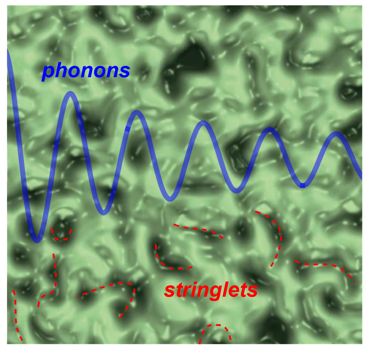
Figure 1: Phonon dynamics in stringlets-land. Acoustic waves interacting with localized 1D string-like objects with exponentially distributed size – “stringlets”. The background of this figure is taken from Wondraczek (2022).

Inspired by the original elastic string model by Granato and Lücke Granato and Lücke (1956), Lund and collaborators have extensively studied the problem of the interplay between elastic phonons and dislocation-like line defects Maurel et al. (2004, 2005a, 2005b); Lund (2015); Churochkin and Lund (2022); Lund (1988), and even pushed it forward as a possible explanation for glassy anomalies Bianchi et al. (2020). In its simplest incarnation, the theory models the defects as a collection of one-dimensional vibrating lines pinned at their extremes and whose length $l$ is distributed according to an unknown function $p(l)$. At the time of Ref. Bianchi et al. (2020), no simulation data for $p(l)$ were available; therefore, Lund et al. Bianchi et al. (2020) through reverse engineering used experimental data for glycerol and silica to extract $p(l)$ and found that a gaussian-shaped distribution would give impressive agreement with the data.

Unfortunately, as we now know from various works Hu and Tanaka (2023, 2022); Zhang et al. (2021); Zhang and Douglas (2013a, b); Douglas et al. (2016); Betancourt et al. (2015), a gaussian-shaped distribution is not compatible with the simulation data that, on the contrary, show a monotonically decreasing exponential distribution of lengths $p(l)\sim\exp(-l/\lambda)$, with possible power-law corrections Pazmino Betancourt et al. (2014). Additionally, without the direct input of $p(l)$ from simulations, the theory in Ref. Bianchi et al. (2020) cannot be fully predictive since $p(l)$ has to be fitted from the data themselves. In Jiang et al. (2023), we have revisited Lund’s model Bianchi et al. (2020) by assuming the correct exponential distribution for the stringlet length and we have found remarkable quantitative agreement with the simulation data of Hu and Tanaka (2023, 2022) using a parameter-free theoretical formula for the BP frequency in the low-temperature glassy phase.

Nonetheless, in Jiang et al. (2023), for simplicity, we have considered phonons and stringlets as independent entities and derived the low-frequency excess anomaly uniquely considering the contribution to the vibrational density of states from the stringlets. Technically, this assumption implies that the total vibrational density of states is just the sum of a Debye phononic contribution and an independent term arising from the stringlet modes. This decoupling of the modes seems to break down at large frequencies where hybridization takes place (see, e.g., Lerner and Bouchbinder (2023)), and it is possibly the responsible for the large uncertainties found when compared to the data at large temperatures, well above the phenomenological glass transition temperature $T_{g}$ (see Jiang et al. (2023) for details).

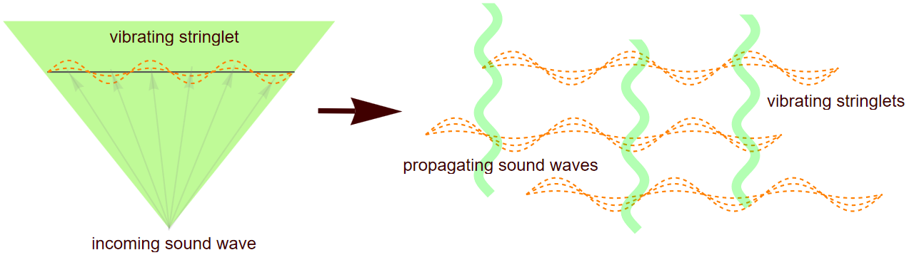
Figure 2: A representation of the theoretical model for stringlet-phonon interactions. An incoming sound wave excites a stringlet that starts vibrating around its equilibrium position. Consequently, sound waves propagate in a bath of vibrating stringlets that strongly renormalize their properties as described by Eq.(1).

In this work, we extend the theoretical model presented in Jiang et al. (2023) by considering the interplay between stringlets and phonons. Among the various advantages of this route, we are now able to predict the effects of the stringlets on the phonon properties such as their propagation speed and their attenuation constant.

II Theoretical model

The theoretical model considered in this work was introduced by Lund and collaborators in a series of works Maurel et al. (2004, 2005a, 2005b); Lund (2015); Churochkin and Lund (2022); Lund (1988); Bianchi et al. (2020). For simplicity, we will use a simplified version of Lund’s model that does not take into account the different phonon polarizations (transverse and longitudinal) and other complications related to the properties of the dislocation-like line defects. In a sense, our model is more similar to the scalar elasticity theory proposed by Granato and Lücke Granato and Lücke (1956). Moreover, we will consider the computation of the phonon self-energy only at leading order in the potential induced by the interactions with the stringlets. As we will explicitly prove, this simplified model is enough to capture the salient physical features. At the same time, its generalization is straightforward and indeed already built by Lund and collaborators in the aforementioned works. Finally, before starting our exposition, we emphasize that the main difference between our analysis on glassy anomalies and the one in Bianchi et al. (2020) relies on the distribution of the stringlet lengths $p(l)$. In Bianchi et al. (2020), the distribution $p(l)$ was not taken as an input of the theory, but rather fitted from the data, leading to an incorrect final result. On the other hand, it is now derived explicitly thanks to the recent simulation progress Hu and Tanaka (2023, 2022); Zhang et al. (2021); Zhang and Douglas (2013a, b); Douglas et al. (2016); Betancourt et al. (2015) that allow for a direct determination of $p(l)$. This also strongly improves the degree of predictability of the theoretical model, as already confirmed in Jiang et al. (2023).

The main idea of this theoretical description, visualized in Fig.2, is that the elastic medium contains one-dimensional string-like defects (stringlets), pinned at their endpoints, that are excited by incoming sound waves and vibrate as a consequence of that. As in a chain reaction, sound waves in the medium now propagate in a bath of vibrating one-dimensional defects that strongly renormalize sound propagation, and the properties of phonons, with crucial consequent effects for the vibrational dynamics of the medium.

As explained in Bianchi et al. (2020), this is equivalent to considering the propagation of sound in a medium with a frequency dependent index of refraction induced in this concrete case by the presence of the stringlets. Neglecting the different longitudinal and transverse polarizations (see Appendix A in Bianchi et al. (2020) for a more complete treatment), the phonon Green function can be written as

$$\mathcal{G}(k,\omega)=\frac{1}{-\omega^{2}+v^{2}k^{2}-i\omega\gamma k^{2}-\Gamma(\omega,k)},$$ (1)

where $\Gamma(\omega,k)$ is the self-energy including the effects coming from the stringlets and $v,\gamma$ are respectively the bare speed of sound and phonon damping. Additionally, $\omega,k$ are the frequency and wave-vector of the phonon. Eq.(1) is the result of a Dyson’s equation,

$$\mathcal{G}(\omega,k)=\left[\mathcal{G}_{0}(\omega,k)^{-1}-\Gamma(\omega,k)\right]^{-1},$$ (2)

where $\mathcal{G}_{0}(\omega,k)$ is the “bare” phonon Green’s function

$$\mathcal{G}_{0}(k,\omega)=\frac{1}{-\omega^{2}+v^{2}k^{2}-i\omega\gamma k^{2}}.$$ (3)

Here, with the label “bare” we mean the phonon propagator before taking into account stringlet-phonon interactions, but taking into account other sources of damping, e.g., phonon-phonon interactions giving rise to Akhiezer damping Akhiezer (1939).

By assuming that the length of the stringlets follow a statistical distribution $p(l)$, and working at leading order in the stringlet potential, one obtains the following expression for the self-energy,

$$\Gamma(\omega,k)=\mu^{2}k^{2}\int_{0}^{\infty}l\,p(l)\,\mathcal{G}_{s}(\omega,l)\,dl,$$ (4)

where $\mathcal{G}_{s}(k,\omega)$ is the bare stringlet Green’s function:

$$\mathcal{G}_{s}(\omega,l)=\frac{1}{-\omega^{2}+v_{s}^{2}(\pi/l)^{2}-i\omega\gamma_{s}}.$$ (5)

Here we have assumed, as in Jiang et al. (2023), that the stringlets vibrate only at their fundamental frequency, $\omega^{(l)}_{s}\equiv\pi v/l$, and neglected all higher harmonics. In Eq.(4), $v_{s}$ and $\gamma_{s}$ are the stringlet propagation speed and attenuation constant that, for the moment, are taken as independent parameters. Moreover, $\mu$ is a phenomenological parameter with units $\left[\sqrt{L}/t^{2}\right]$ that parametrizes the strength of the interactions between stringlets and phonons, and that can be eventually related to microscopic physics observables Bianchi et al. (2020). For simplicity, in this work, we will take it as an adjustable parameter. To avoid clutter, we do not repeat the derivation of Eq.(4) here but refer the Readers to Appendix A of Bianchi et al. (2020). Our equation (4) can be directly compared with Eq.(A.14) therein by identifying $f(\omega)k^{2}\equiv\Gamma(\omega,k)$, $v^{2}f_{0}\equiv\mu^{2}$, and by neglecting the term proportional to $\omega^{3}$ in the denominator of Eq.(A.14) that comes from second order perturbation theory.

Having the renormalized Green’s function, several other properties of phonons in “stringlet-land” follow. More precisely, the dynamic structure factor can be then obtained as,

$$S(\omega,k)=\dfrac{1}{\pi}\mathrm{Im}[\mathcal{G}(\omega,k)].$$ (6)

The phonon vibrational density of states (VDOS) is then given by,

$$g(\omega)=\dfrac{2\omega}{k_{D}^{3}\pi}\int_{0}^{k_{D}}\mathrm{Im}[\mathcal{G}(\omega,k)]k^{2}dk,$$ (7)

where $k_{D}$ is the Debye wave-vector. Finally, the real and imaginary parts of the self-energy $\Gamma(\omega,k)$ renormalize the bare speed of sound $v$ and the bare attenuation constant $\gamma$ respectively. Even more drastically, the renormalized Green’s function in Eq.(1) will contain a more complex pole structures than its bare counterpart, leading to the presence of a flat BP mode.

Before continuing with the results, let us establish our main assumption that is an exponential distribution of the stringlet lengths given by:

$$p(l)=p_{0}e^{-l/\lambda},$$ (8)

where $p_{0}$ is a normalization factor and $\lambda$ the average stringlet length $\lambda\equiv\langle l\rangle$. We notice that Eq.(8) is consistent with several simulation results Hu and Tanaka (2023, 2022); Zhang et al. (2021); Zhang and Douglas (2013a, b); Douglas et al. (2016); Betancourt et al. (2015), and has already been successfully used in the prediction of the BP frequency in the low-temperature glassy state Jiang et al. (2023). Let us clarify that the stringlet length $l$ does not vary in the interval $[0,\infty]$ but presents a natural IR cutoff in the sample size $L$, and a natural UV cutoff in the atomic distance $a$. As a consequence, the stringlet size distribution in Eq.(8) has to be limited within the range $a\ll l\ll L$. However, in realistic situations, the average stringlet length, that will set the boson peak scale, is of the order of nanometers, far away from both cutoffs. This implies that the effects of the cutoffs become important only for frequencies much smaller and much larger than the BP frequency, and are therefore irrelevant for the present discussion.

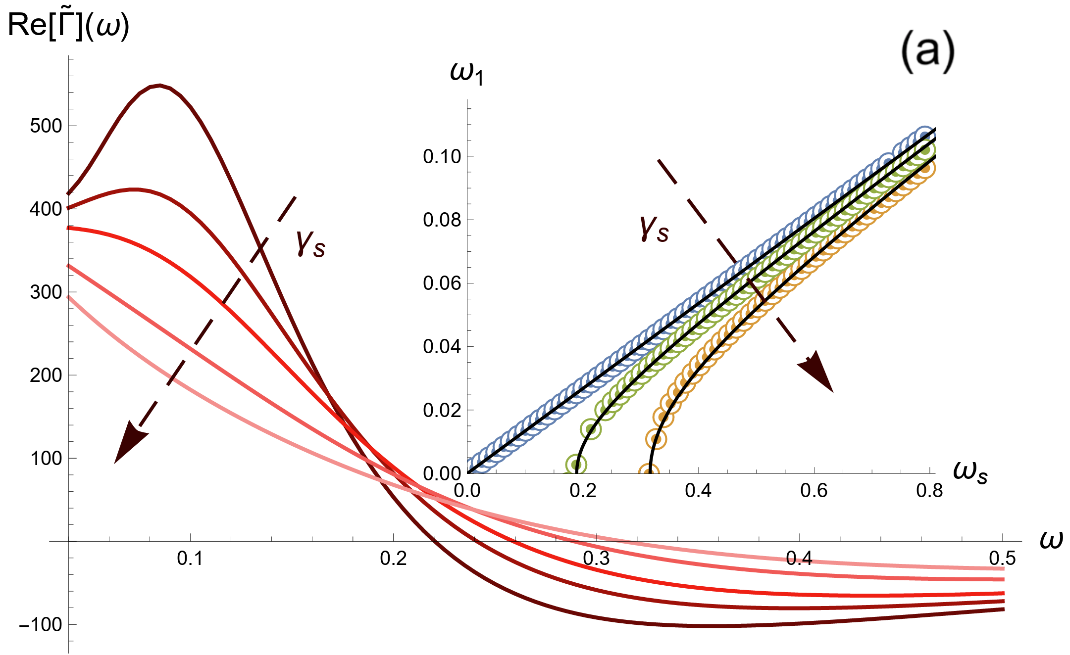
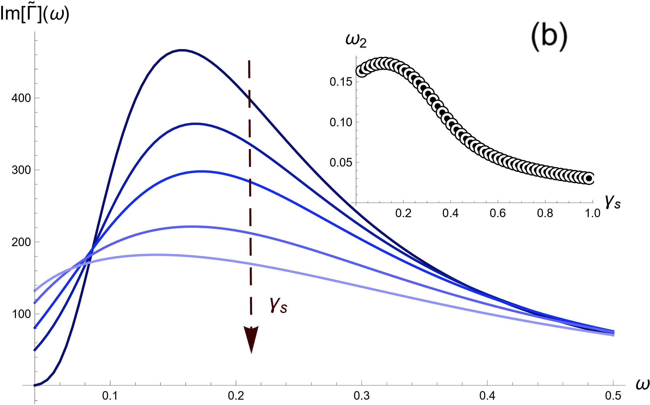
Figure 3: The phonon self energy. (a) The real part of the reduced self energy $\tilde{\Gamma}(\omega)$ as a function of the frequency for $v_{s}=1$, $\lambda=5$ and different values of $\gamma_{s}=0,0.05,0.1,0.2,0.3$ from dark to light red. The inset shows the frequency of the maximum $\omega_{1}$ as a function of the average stringlet frequency $\omega_{s}$ for $\gamma_{s}=0,0.03,0.05$. The black lines are the fits discussed in the main text. (b) The imaginary part of $\tilde{\Gamma}(\omega)$ as a function of $\omega$ for the same values of $\gamma_{s}$ as in the top panel. The inset shows the frequency of the maximum $\omega_{2}$ as a function of the stringlet damping $\gamma_{s}$.

III Results

III.1 Phonon self-energy

Our theoretical analysis starts with a detailed investigation of the phonon self-energy $\Gamma(\omega,k)$. To limit the number of unknown parameters, we neglect the effects of the phonon damping $\gamma$, and we set it to zero if not indicated otherwise. Moreover, to simplify the presentation, we define a renormalized self-energy

$$\tilde{\Gamma}(\omega)\equiv\frac{\Gamma(\omega,k)}{\mu^{2}k^{2}},$$ (9)

which now depends only on the frequency $\omega$ and it is independent of the coupling strength $\mu$. The real and imaginary parts of this renormalized self-energy are plotted as a function of frequency in Fig.3 for various values of the stringlet damping parameter $\gamma_{s}$. For further discussion, we define with

$$\omega_{1}\equiv\max_{\{\omega\}}\mathrm{Re}\tilde{\Gamma}(\omega),\qquad\omega_{2}\equiv\max_{\{\omega\}}\mathrm{Im}\tilde{\Gamma}(\omega),$$ (10)

the values of the frequency at which the real and imaginary parts of the renormalized self-energy attain their maximum. The imaginary part of $\tilde{\Gamma}$ displays a peak that, in the limit of zero stringlet damping, is analytically given by the following expression

$$\omega_{2}(\gamma_{s}=0)=\frac{\pi v_{s}}{4\lambda}=\frac{\omega_{s}}{4}.$$ (11)

Interestingly, this expression coincides exactly with the theoretical prediction for the BP frequency in the stringlet model of Jiang et al. (2023), which resulted in good agreement with the simulation data at low temperature (where the damping mechanisms can be neglected). This peak is consistently broadened by increasing the stringlet damping and its position follows a non-monotonic function shown in the inset of the bottom panel of Fig.3.

The behavior of the real part of the renormalized self-energy $\tilde{\Gamma}$ as a function of frequency is more complex. Its trend is characterized by a constant zero frequency value, a possible intermediate peak and high-frequency regime in which the function takes negative values. In the limit of zero stringlet damping, the intermediate peak frequency $\omega_{1}$ is a linear function of the average stringlet frequency $\omega_{s}\equiv v\pi/\lambda$. More in general, we find that the intermediate peak frequency in first approximation follows

$$\omega_{1}\approx\sqrt{\omega_{s}^{2}-\zeta},$$ (12)

where $\zeta$ is a phenomenological parameter that vanishes in absence of stringlet damping, and grows with the latter. We notice that this functional form implies a crossover from an underdamped regime in which the real part of $\tilde{\Gamma}$ shows a distinct and sharp maximum, to an overdamped regime in which it decays monotonically with the frequency $\omega$.

III.2 Dynamic structure factor

Starting from the self-energy, we can directly derive the phonon Green function, Eq.(1), and consequently the dynamic structure factor, Eq.(6).

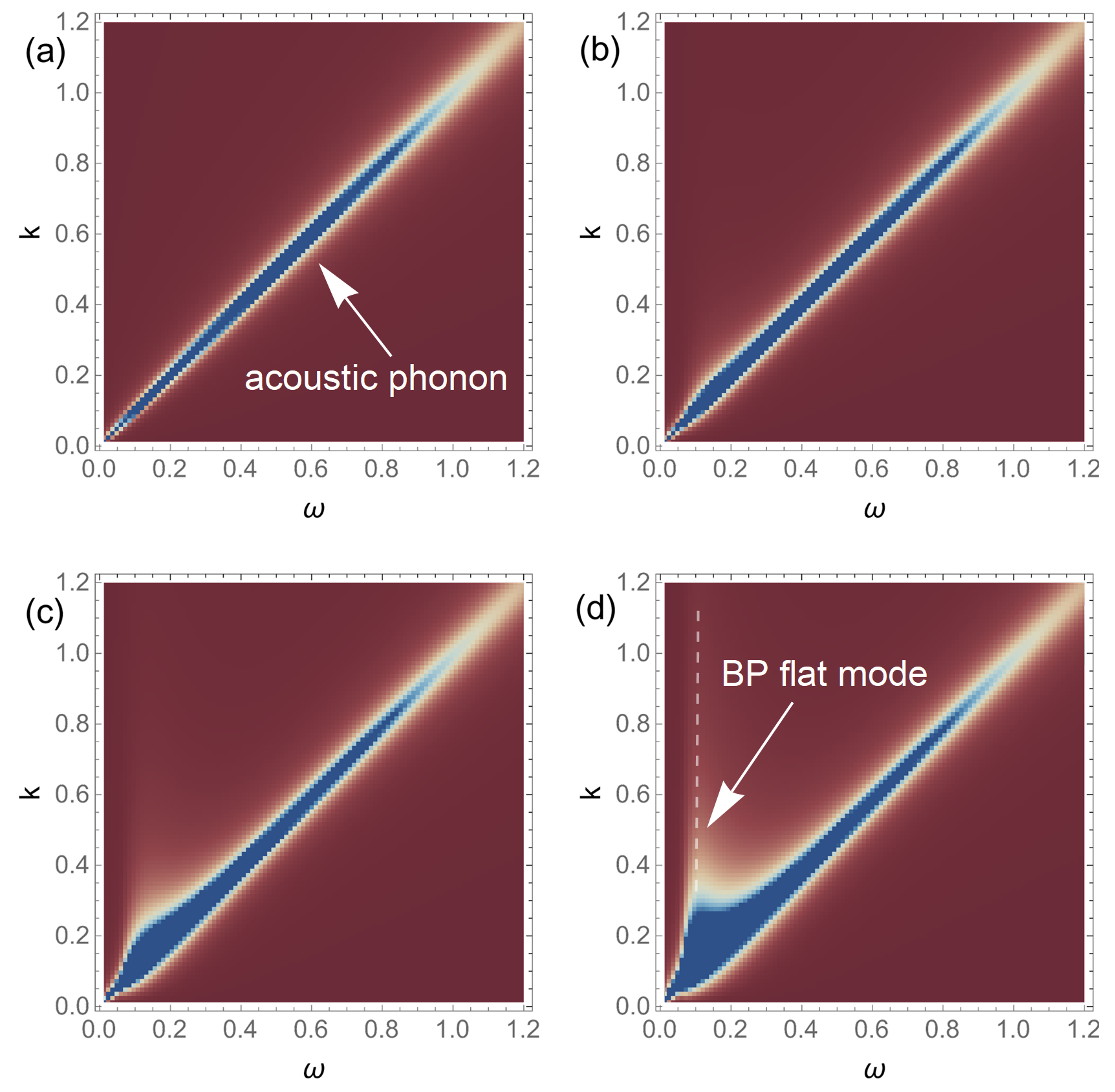
Figure 4: Emergence of a BP flat mode. The dynamical structure factor $S(\omega,k)$ for $\mu=0,0.01,0.02,0.03$ from (a) to (d). From red to blue the intensity is stronger. Other parameters involved here are $v=v_{s}=1$, $\lambda=5$, $\gamma=\gamma_{s}=10^{-8}$. The vertical dashed line in panel (d) highlights the flat dispersion of the BP mode that is confirmed by constant $k$ cuts of $S(\omega,k)$ shown in Fig.5.

If we neglect the interactions between the stringlet degrees of freedom and the acoustic phonons, i.e., $\mu=0$, the dynamic structure factor simply reads

$$S(\omega,k)_{\mu=0}=\frac{\omega\,\gamma\,k^{2}}{\pi\,\left[\left(\omega^{2}-v^{2}k^{2}\right)^{2}+\gamma^{2}\omega^{2}\,k^{4}\right]}.$$ (13)

This case is shown in panel (a) of Fig.4. The linear dispersion of the damped acoustic phonon is evident.

By increasing the interaction strength $\mu$, the stringlets start dressing the phonon propagator as progressively shown moving from panel (a) to panel (d) in Fig.4. For large enough coupling, panel (d) in Fig.4, a dispersionless flat mode emerges below the phonon frequency. As we will see in the next section, the energy of this flat mode coincides with the BP frequency in the reduced density of states. Because of this reason, we label this mode “the BP mode”.

In order to confirm the existence and properties of the BP mode, in Fig.5, we show several cuts of the dynamic structure factor at fixed wave-vector $k$ and varying frequency using the same parameters as in panel (d) of Fig.4. The existence of a dispersionaless mode, in addition to the propagating acoustic phonon, is clear from that representation. Let us also notice that the BP mode exists only for frequencies below the phonon frequency. Its flat dispersion ends on the linear dispersion of the acoustic phonon.

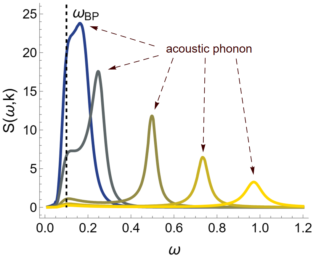
Figure 5: The BP mode in the dynamical structure factor. The dynamical structure factor for $k=0.2,0.4,0.6,0.8$ from dark to light color. Other parameters are same as Fig.4 (d). The vertical dashed line indicates the position of the dispersionless BP mode coinciding with $\omega_{\text{BP}}$. The peak corresponding to the acoustic phonon is also indicated.

All the aforementioned properties of the flat BP mode are consistent with what observed in simulations by Hu and Tanaka Hu and Tanaka (2022). The existence of a flat mode, responsible for the BP anomaly, has also been experimentally observed, see for example Tømterud et al. (2023). As a general remark, we highlight that from a macroscopic perspective (but certainly not from a microscopic point of view) the existence of such a flat mode is similar to the appearance of low-energy optical modes, that have been identified as the origin of the BP in several crystalline materials Moratalla et al. (2019); Baggioli and Zaccone (2019b); Krivchikov et al. (2022).

III.3 Density of states and boson peak

The most direct way to study the properties of BP is to investigate the reduced VDOS, $g(\omega)/\omega^{d-1}$, where $\omega^{d-1}$ is the scaling predicted by Debye law and $d$ the spatial dimension of system.

In Fig.6, we show the reduced VDOS as a function of the frequency for different values of the stringlet-phonon coupling $\mu$. The gray line shows the result of the pure Debye model with $\omega_{D}=1$. By increasing the coupling strength $\mu$, two phenomena are evident. First, the Debye level at low frequency increases. This is simply the consequence of the renormalization of the phonon speed of propagation, that gets smaller by enhancing the interactions with the stringlets acting as scatterers. Second, and most importantly, a clear BP excess anomaly emerges. The position of this anomaly, $\omega_{\text{BP}}$, coincides exactly with the energy of the flat mode reported in Fig.4 and Fig.5. The intensity of this anomaly becomes larger by increasing the coupling strength, while its position is only mildly dependent on it. The position is indeed mostly controlled by the average stringlet length (that is kept fixed in Fig.6) and the phonon propagation speed (also fixed therein).

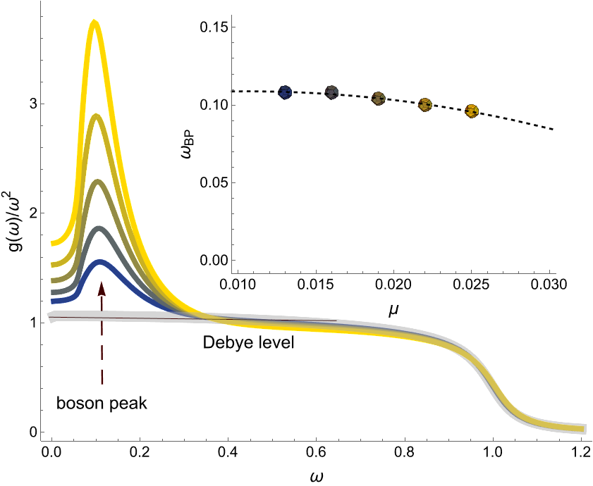
Figure 6: The boson peak. The Debye reduced VDOS for different values of the stringlet-phonon coupling $\mu=0.03,0.05,0.07,0.09,0.11$ (from blue to yellow). The parameters are fixed to $v=v_{s}=1$, $k_{D}=1$, $\lambda=5$ and $\gamma=\gamma_{s}=10^{-8}$. The gray line is the result for $\mu=0$ displaying the case of the pure Debye model. The inset shows the trend of the BP frequency as a function of $\mu$.

The theoretical model at hand allows for a broad investigation of the BP properties as a function of the various parameters. In Fig.7, we show some of these properties as a function of the phonon-stringlet strength and the phonon speed of propagation. In particular, we focus on the BP frequency, defined as the maximum in the reduced VDOS $g(\omega)/\omega^{2}$ and the BP intensity $I_{\text{BP}}$,

$$I_{\text{BP}}=\frac{g(\omega)}{\omega^{2}}|_{\omega_{\text{BP}}}.$$ (14)

To reduce the number of parameters, the speed of stringlet propagation $v_{s}$ is always considered to be same as the speed of sound $v$. At the same time, the damping parameters $\gamma,\gamma_{s}$ are kept fixed to a small value (see caption of Fig.7 for details).

In panel (a) of Fig.7, we observe that the BP frequency decreases monotonically by increasing the stringlet-phonon coupling $\mu$. Nevertheless, its value depends only mildly on $\mu$ and it is mostly controlled by the average stringlet length $\lambda$ and the stringlet speed $v_{s}$, consistent with the findings in Jiang et al. (2023).

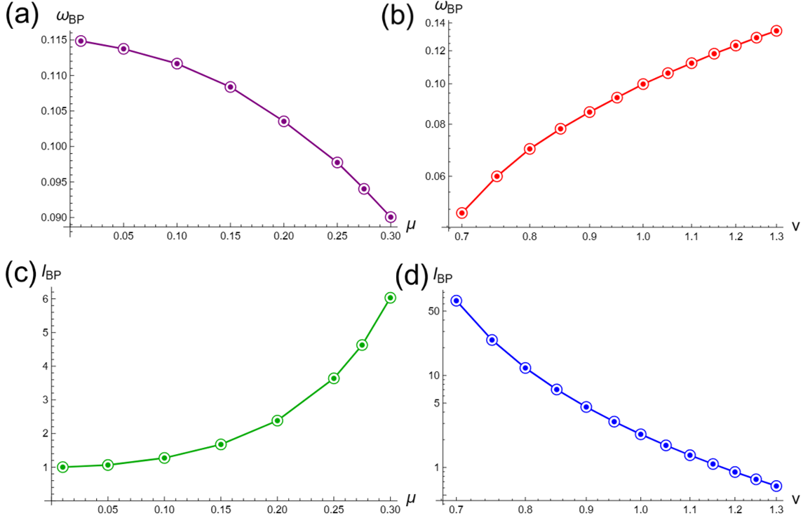
Figure 7: BP properties. The BP frequency and intensity as a function of the stringlet-phonon coupling $\mu$, panels (a) and (c), and the propagation speed $v=v_{s}$, panels (b) and (d). In panels (a) and (d) we fix $v=v_{s}=1$, $k_{D}=1$, $\lambda=5$, $\gamma=10^{-3}$ and $\gamma_{s}=10^{-2}$. In panels (b) and (d) we fix $\mu=0.02$ and $v=v_{s}$ is taken as a free parameter.

On the contrary, as shown in panel (b) of Fig.7, $\omega_{\text{BP}}$ grows monotonically by increasing the speed of sound $v$, which is taken to coincide with the stringlet speed $v=v_{s}$.

In panels (c)-(d) of Fig.7, we show how the BP intensity, defined in Eq.(14), depends on the same parameters. We observe that the coupling strength $\mu$ and the propagation speed $v$ have an opposite effect on $I_{\text{BP}}$. The BP signal becomes stronger by increasing $\mu$, while it gets weaker by increasing $v$. We notice that this last behavior is consistent with the trend of the experimental data, e.g. Kawashima et al. (2009).

Finally, we find that by increasing the damping parameters $\gamma$, $\gamma_{s}$ (data not shown in Fig.7), the BP frequency is also softened, in agreement with the results in Jiang et al. (2023).

III.4 Sound attenuation and effective phonons speed

The effective dispersion relation of the acoustic phonons can be obtained by considering the poles of the dressed propagator Eq.(1),

$$-\omega^{2}+v^{2}k^{2}-i\omega\gamma k^{2}-\mu^{2}k^{2}\tilde{\Gamma}(\omega)=0.$$ (15)

We treat the wavevector $k$ as a complex number and we set the frequency $\omega$ to be a real number. Then, the equation above can be recasted as,

$$k^{2}\left(v^{2}-i\omega\gamma-\mu^{2}\tilde{\Gamma}(\omega)\right)-\omega^{2}=0.$$ (16)

Therefore, the effective dispersion relation is

$$k(\omega)=\dfrac{\omega}{\sqrt{v^{2}-i\omega\gamma-\mu^{2}\tilde{\Gamma}(\omega)}}\equiv k_{1}(\omega)+ik_{2}(\omega).$$ (17)

Following standard definitions, the effective speed of sound can be obtained as:

$$v_{\text{eff}}(\omega)=\left(\frac{dk_{1}(\omega)}{d\omega}\right)^{-1},$$ (18)

and the sound attenuation length is defined as the inverse of imaginary part of the wave-vector,

$$l(\omega)=\frac{1}{k_{2}(\omega)}.$$ (19)

In absence of stringlet-phonon interactions, $\mu=0$,

$$k_{1}(\omega)=\frac{\omega\cos\left(\frac{1}{2}\arg\left(v^{2}-i\gamma\omega\right)\right)}{\sqrt[4]{v^{4}+\gamma^{2}\omega^{2}}},$$ (20)

$$k_{2}(\omega)=-\frac{\omega\sin\left(\frac{1}{2}\arg\left(v^{2}-i\gamma\omega\right)\right)}{\sqrt[4]{v^{4}+\gamma^{2}\omega^{2}}}.$$ (21)

In that case, $\gamma=0$ implies that $k_{2}(\omega)=0$ and $k_{1}(\omega)=\omega/v$ as expected. Two examples of $l(\omega)$ and $v_{\text{eff}}(\omega)$ following from Eqs.(20)-(21) are shown in Fig.8 in gray color.

In Fig.8 we show the sound attenuation length and the effective sound velocity as a function of the frequency by dialing the stringlet-phonon coupling $\mu$. The first visible feature is that the sound attenuation length diverges at $\omega=0$. This is simply the consequence of the absence of any scattering or damping mechanism that remains active in the limit of zero frequency. In other words, the imaginary part of the phonon propagator vanishes at $\omega=0$. A second property is that the larger $\mu$ the shorter attenuation length, that is compatible with $\mu$ determining the amount of interaction/scattering between stringlets and phonons.

More in general, we observe that the stringlets renormalize strongly the phonon properties only in a frequency window around the BP energy. The sound attenuation length is strongly decreased slightly above the BP frequency, in the interval $\omega_{\text{BP}}<\omega<0.4$ in Fig.8.

The effective phonon velocity is also strongly modified by the coupling with the stringlets. In particular, as evident from the inset in Fig.8, the speed of sound is decreased slightly below the BP frequency and increased slightly above it.

Finally, for large frequencies, the interactions with the stringlets become subleading and both the sound attenuation and the effective speed approach their $\mu=0$ values.

The picture just presented is consistent with the results of Bianchi et al. (2020), proving that this phenomenology is quite insensitive to the precise form of the stringlet size distribution, aside from the information about the average length $\lambda$.

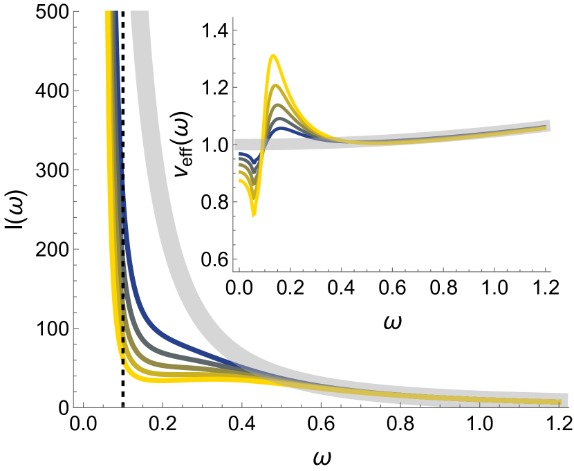
Figure 8: Phonon propagation in stringlet-land. The sound attenuation length $l(\omega)$ and effective speed of propagation $v_{\text{eff}}(\omega)$ as a function of the frequency for increasing values of the stringlet-phonon coupling $\mu$. The gray lines correspond to the results for $\mu=0$. The other parameters involved here are the same as Fig.6 (the color scheme is also matched).

III.5 The length scale associated to the boson peak

The idea of associating a length-scale to the BP is certainly not new and has been explored in various directions, e.g., Granato (1992); Hong et al. (2011a, b); Kalampounias et al. (2006); Malinovsky et al. (1988); Malinovsky and Sokolov (1986); Martin and Brenig (1974).

From a macroscopic perspective, in the spirit of heterogeneous elasticity theory Schirmacher and Ruocco , the BP scale can be identified from the disordered distribution of the shear modulus. In other words, the length scale is the average size of the shear modulus fluctuations in the disordered solid. From a more microscopic perspective, the same length scale can be thought as arising from quasi-localized structures coexisting with phonons in amorphous materials Lerner and Bouchbinder (2021). In this context, the length scale corresponds to the average size of these “defects” that punctuate the otherwise homogeneous elastic medium. Interestingly, a direct quantitative relation between the scales defined using these two approaches has been confirmed in certain glass models Mahajan and Ciamarra (2021), providing a possible “peace treaty” between the two parts.

According to the stringlet theory of the boson peak Mahajan and Ciamarra (2021), the length-scale associated with the BP is the average stringlet size, determined by the stringlet length distribution $p(l)$. As shown by means of simulations in Hu and Tanaka (2022), and now proved theoretically (see Fig.4), stringlet-phonon interactions induce the emergence of a flat BP mode. We notice that, because of its non-dispersive character and its low-energy compared to that of acoustic phonons, it is conceivable to interpret such a mode as a quasi-localised low-energy excitation. We notice that the analysis in Hu and Tanaka (2022) suggests that this BP mode mode is unrelated to the quadrupolar four-leaf defects discussed in the literature, that appear somehow at frequencies much below the BP scale, but this debate has not been settled yet Lerner and Bouchbinder (2023).

Let us go back to the dressed phonon Green’s function in Eq.(1). From there, we observe that the phonon speed is renormalized by the self-energy $\Gamma(\omega,k)$,

$$\tilde{v}^{2}(k)=v^{2}-\dfrac{\mathrm{Re}[\Gamma(\omega(k),k)]}{k^{2}}.$$ (22)

Here, we have used the dispersion relation $\omega(k)$ to make the renormalized speed a function of only the wave-vector $k$. At this point, it is straightforward to Fourier transform $\tilde{v}^{2}(k)$ back into real space and define a space-dependent phonon speed,

$$\tilde{v}^{2}(x)=\mathcal{F}\left[\tilde{v}^{2}(k)\right].$$ (23)

Microscopically, the heterogeneous nature of the phonon speed of propagation is just a direct consequence of the framework depicted in Fig.1, in which the phonons propagate in a bath of vibrating stringlets with different sizes. After a coarse-graining procedure, that is technically realized via solving the Dyson’s equations and integrating out the stringlet degrees of freedom, $\tilde{v}^{2}(x)$ is one of the macroscopic effects remaining.

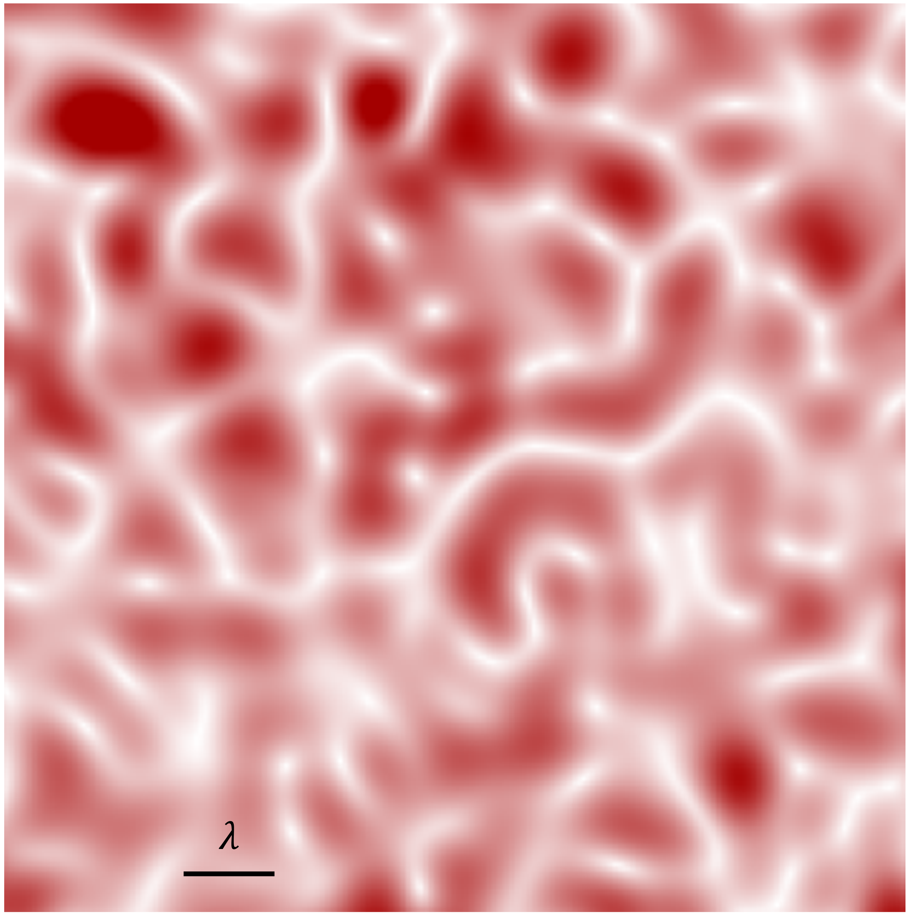
Figure 9: From stringlets to heterogeneous dynamics. The heterogeneous phonon speed $\tilde{v}^{2}(x)$ in real space. The color map indicates its intensity from white to red color. The black line indicates the scale of $\lambda$ used to realize this figure.

In Fig.9, we provide a visual representation of this effect by using a benchmark value for the average stringlet length $\lambda$. Red color indicates spatial regions in which the phonon speed is large. The correlation between the average size of the fluctuations of $\tilde{v}^{2}(x)$ and $\lambda$ is evident, and perhaps not surprising. This simple analysis suggests that the ideas that the BP scale is set by the fluctuations of heterogeneous elasticity or by the average size of localized defects (whatever their microscopic origin is) are not incompatible. Indeed, in our view, they are just different approaches towards the same problem, one more macroscopic and effective, while the other more microscopic.

IV Outlook and discussion

In this work, we studied the dynamical and vibrational properties of an idealized amorphous solid modelled as an elastic medium punctuated by pinned elastic string-like obects (stringlets) with exponentially distributed length. The theoretical framework is a generalization of Lund’s theory Bianchi et al. (2020) that uses an exponential stringlet size distribution verified by simulations. Despite the simplicity of the model, the results qualitatively agree with the observed BP properties and, together with Jiang et al. (2023), provide a theoretical ground for the recent simulation observations by Hu and Tanaka Hu and Tanaka (2022, 2023).

Several open questions remain. In particular, at present, the emergent nature of the stringlets remains unclear. Stringlets are certainly not fundamental vibrational excitations but rather an emergent collective phenomenon that arises probably because of interactions and anharmonicity. The fundamental origin of the stringlets, and the statistical mechanics reasoning behind their appearance itself, are still matter of investigation. Moreover, from a theoretical point of view, it is not obvious to understand why in a 3D amorphous solid, the fundamental objects behind the BP anomaly should be of 1D nature. At this moment, this seems to be only a simplifying working assumption that needs further corroboration.

Finally, the emergence of a BP flat mode is a very appealing feature. First, this is in common among various theoretical approaches including heterogeneous elasticity theory and quasi-localized modes. Second, this feature is observed not only in simulations Hu and Tanaka (2022) but even in experiments Tømterud et al. (2023). Third, from a macroscopic point of view, this feature is strikingly similar to the existence of low-lying optical modes that have been ascribed as the origin of the BP anomaly in crystalline materials Moratalla et al. (2019); Baggioli and Zaccone (2019b); Krivchikov et al. (2022), hinting toward a possible macroscopic (but not microscopic) universal framework. Along these lines, stringlets have been indeed already discussed as the responsible for the BP anomaly in heated crystals by Douglas and collaborators Zhang and Douglas (2013b, a). These analogies certainly deserve more attention in the near future.

References

- Debye (1912) P. Debye, Annalen der Physik 344, 789 (1912).
- Leutwyler (1997) H. Leutwyler, Helv. Phys. Acta 70, 275 (1997), arXiv:hep-ph/9609466 .
- Kittel (2021) C. Kittel, Introduction to solid state physics Eighth edition (2021).
- Ramos (2022) M. A. Ramos, Low-temperature Thermal and Vibrational Properties of Disordered Solids: A Half-century of Universal” anomalies” of Glasses (World Scientific, 2022).
- Ackerman et al. (1981) D. A. Ackerman, D. Moy, R. C. Potter, A. C. Anderson, and W. N. Lawless, Phys. Rev. B 23, 3886 (1981).
- Takabatake et al. (2014) T. Takabatake, K. Suekuni, T. Nakayama, and E. Kaneshita, Rev. Mod. Phys. 86, 669 (2014).
- Schliesser and Woodfield (2015) J. M. Schliesser and B. F. Woodfield, Journal of Physics: Condensed Matter 27, 285402 (2015).
- Moratalla et al. (2019) M. Moratalla, J. F. Gebbia, M. A. Ramos, L. C. Pardo, S. Mukhopadhyay, S. Rudić, F. Fernandez-Alonso, F. J. Bermejo, and J. L. Tamarit, Phys. Rev. B 99, 024301 (2019).
- Elliott (1992) S. R. Elliott, Europhysics Letters 19, 201 (1992).
- Schirmacher (2006) W. Schirmacher, Europhysics Letters 73, 892 (2006).
- Schirmacher et al. (2007) W. Schirmacher, G. Ruocco, and T. Scopigno, Phys. Rev. Lett. 98, 025501 (2007).
- Schirmacher et al. (2015) W. Schirmacher, G. Ruocco, and V. Mazzone, Phys. Rev. Lett. 115, 015901 (2015).
- Léonforte et al. (2006) F. Léonforte, A. Tanguy, J. P. Wittmer, and J.-L. Barrat, Phys. Rev. Lett. 97, 055501 (2006).
- Buchenau et al. (1991) U. Buchenau, Y. M. Galperin, V. L. Gurevich, and H. R. Schober, Phys. Rev. B 43, 5039 (1991).
- Gurevich et al. (2003) V. L. Gurevich, D. A. Parshin, and H. R. Schober, Phys. Rev. B 67, 094203 (2003).
- Parshin et al. (2007) D. A. Parshin, H. R. Schober, and V. L. Gurevich, Phys. Rev. B 76, 064206 (2007).
- Götze and Mayr (2000) W. Götze and M. R. Mayr, Phys. Rev. E 61, 587 (2000).
- Baggioli and Zaccone (2019a) M. Baggioli and A. Zaccone, Phys. Rev. Lett. 122, 145501 (2019a).
- Taraskin et al. (2001) S. N. Taraskin, Y. L. Loh, G. Natarajan, and S. R. Elliott, Phys. Rev. Lett. 86, 1255 (2001).
- Chumakov et al. (2011) A. I. Chumakov, G. Monaco, A. Monaco, W. A. Crichton, A. Bosak, R. Rüffer, A. Meyer, F. Kargl, L. Comez, D. Fioretto, H. Giefers, S. Roitsch, G. Wortmann, M. H. Manghnani, A. Hushur, Q. Williams, J. Balogh, K. Parliński, P. Jochym, and P. Piekarz, Phys. Rev. Lett. 106, 225501 (2011).
- Galperin et al. (1989) Y. Galperin, V. Karpov, and V. Kozub, Advances in Physics 38, 669 (1989).
- Klinger and Kosevich (2002) M. Klinger and A. Kosevich, Physics Letters A 295, 311 (2002).
- Grigera et al. (2003) T. S. Grigera, V. Martín-Mayor, G. Parisi, and P. Verrocchio, Nature 422, 289 (2003).
- Jiang et al. (2023) C. Jiang, M. Baggioli, and J. F. Douglas, arXiv preprint arXiv:2311.04230 (2023).
- Schober and Oligschleger (1996) H. R. Schober and C. Oligschleger, Phys. Rev. B 53, 11469 (1996).
- Lerner and Bouchbinder (2023) E. Lerner and E. Bouchbinder, The Journal of Chemical Physics 158, 194503 (2023).
- Rainone et al. (2021) C. Rainone, P. Urbani, F. Zamponi, E. Lerner, , and E. Bouchbinder, SciPost Phys. Core 4, 008 (2021).
- Vural and Leggett (2011) D. Vural and A. Leggett, Journal of Non-Crystalline Solids 357, 3528 (2011).
- Schober et al. (1993) H. Schober, C. Oligschleger, and B. Laird, Journal of Non-Crystalline Solids 156-158, 965 (1993).
- Hu and Tanaka (2023) Y.-C. Hu and H. Tanaka, Phys. Rev. Res. 5, 023055 (2023).
- Hu and Tanaka (2022) Y.-C. Hu and H. Tanaka, Nature Physics 18, 669 (2022).
- Zhang et al. (2021) H. Zhang, X. Wang, H.-B. Yu, and J. F. Douglas, The Journal of Chemical Physics 154, 084505 (2021).
- Zhang and Douglas (2013a) H. Zhang and J. F. Douglas, Soft Matter 9, 1254 (2013a).
- Zhang and Douglas (2013b) H. Zhang and J. F. Douglas, Soft Matter 9, 1266 (2013b).
- Douglas et al. (2016) J. F. Douglas, B. A. P. Betancourt, X. Tong, and H. Zhang, Journal of Statistical Mechanics: Theory and Experiment 2016, 054048 (2016).
- Betancourt et al. (2015) B. A. P. Betancourt, P. Z. Hanakata, F. W. Starr, and J. F. Douglas, Proceedings of the National Academy of Sciences 112, 2966 (2015).
- Novikov and Surovtsev (1999) V. N. Novikov and N. V. Surovtsev, Phys. Rev. B 59, 38 (1999).
- Karpov (1993) V. G. Karpov, Phys. Rev. B 48, 12539 (1993).
- Novikov (1990) V. Novikov, JETP Lett. 51 (1990).
- Angell (2004) C. A. Angell, Journal of Physics: Condensed Matter 16, S5153 (2004).
- Bhat et al. (2006) M. H. Bhat, I. Peral, J. R. Copley, and C. A. Angell, Journal of Non-Crystalline Solids 352, 4517 (2006).
- Kleman and Friedel (2008) M. Kleman and J. Friedel, Rev. Mod. Phys. 80, 61 (2008).
- Cao et al. (2018) Y. Cao, J. Li, B. Kou, C. Xia, Z. Li, R. Chen, H. Xie, T. Xiao, W. Kob, L. Hong, J. Zhang, and Y. Wang, Nature Communications 9, 2911 (2018).
- Baggioli et al. (2021) M. Baggioli, I. Kriuchevskyi, T. W. Sirk, and A. Zaccone, Phys. Rev. Lett. 127, 015501 (2021).
- Baggioli (2023) M. Baggioli, Nature Communications 14, 2956 (2023).
- Baggioli et al. (2022) M. Baggioli, M. Landry, and A. Zaccone, Phys. Rev. E 105, 024602 (2022).
- Wu et al. (2023) Z. W. Wu, Y. Chen, W.-H. Wang, W. Kob, and L. Xu, Nature Communications 14, 2955 (2023).
- Desmarchelier et al. (2024) P. Desmarchelier, S. Fajardo, and M. L. Falk, arXiv preprint arXiv:2401.07109 (2024).
- Bera et al. (2024) A. Bera, M. Baggioli, T. C. Petersen, T. W. Sirk, A. C. Liu, and A. Zaccone, arXiv preprint arXiv:2401.15359 (2024).
- Wondraczek (2022) L. Wondraczek, Nature Physics 18, 614 (2022).
- Granato and Lücke (1956) A. Granato and K. Lücke, Journal of Applied Physics 27, 583 (1956).
- Maurel et al. (2004) A. Maurel, J.-F. m. c. Mercier, and F. Lund, Phys. Rev. B 70, 024303 (2004).
- Maurel et al. (2005a) A. Maurel, V. Pagneux, F. Barra, and F. Lund, Phys. Rev. B 72, 174110 (2005a).
- Maurel et al. (2005b) A. Maurel, V. Pagneux, F. Barra, and F. Lund, Phys. Rev. B 72, 174111 (2005b).
- Lund (2015) F. Lund, Phys. Rev. B 91, 094102 (2015).
- Churochkin and Lund (2022) D. Churochkin and F. Lund, Phys. Rev. B 106, 024105 (2022).
- Lund (1988) F. Lund, Journal of Materials Research 3, 280 (1988).
- Bianchi et al. (2020) E. Bianchi, V. M. Giordano, and F. Lund, Phys. Rev. B 101, 174311 (2020).
- Pazmino Betancourt et al. (2014) B. A. Pazmino Betancourt, J. F. Douglas, and F. W. Starr, Journal of Chemical Physics 140, 204509 (2014).
- Akhiezer (1939) A. I. Akhiezer, J. Phys. (Moscow) 1, 277 (1939).
- Tømterud et al. (2023) M. Tømterud, S. D. Eder, C. Büchner, L. Wondraczek, I. Simonsen, W. Schirmacher, J. R. Manson, and B. Holst, Nature Physics 19, 1910 (2023).
- Baggioli and Zaccone (2019b) M. Baggioli and A. Zaccone, Journal of Physics: Materials 3, 015004 (2019b).
- Krivchikov et al. (2022) A. I. Krivchikov, A. Jeżowski, D. Szewczyk, O. A. Korolyuk, O. O. Romantsova, L. M. Buravtseva, C. Cazorla, and J. L. Tamarit, Journal of Physical Chemistry Letters 13, 5061 (2022), pMID: 35652901.
- Kawashima et al. (2009) M. Kawashima, Y. Matsuda, Y. Fukawa, M. Kodama, and S. Kojima, Physics and Chemistry of Glasses: European Journal of Glass Science and Technology B 50, 95 (2009).
- Granato (1992) A. V. Granato, Phys. Rev. Lett. 68, 974 (1992).
- Hong et al. (2011a) L. Hong, V. N. Novikov, and A. P. Sokolov, Phys. Rev. E 83, 061508 (2011a).
- Hong et al. (2011b) L. Hong, V. Novikov, and A. Sokolov, Journal of Non-Crystalline Solids 357, 351 (2011b).
- Kalampounias et al. (2006) A. G. Kalampounias, S. N. Yannopoulos, and G. N. Papatheodorou, The Journal of Chemical Physics 125, 164502 (2006).
- Malinovsky et al. (1988) V. Malinovsky, V. Novikov, A. Sokolov, and V. Bagryansky, Chemical Physics Letters 143, 111 (1988).
- Malinovsky and Sokolov (1986) V. Malinovsky and A. Sokolov, Solid State Communications 57, 757 (1986).
- Martin and Brenig (1974) A. J. Martin and W. Brenig, physica status solidi (b) 64, 163 (1974).
- (72) W. Schirmacher and G. Ruocco, “Heterogeneous elasticity: The tale of the boson peak,” in Low-Temperature Thermal and Vibrational Properties of Disordered Solids, Chap. Chapter 9, pp. 331–373.
- Lerner and Bouchbinder (2021) E. Lerner and E. Bouchbinder, The Journal of Chemical Physics 155, 200901 (2021).
- Mahajan and Ciamarra (2021) S. Mahajan and M. P. Ciamarra, Phys. Rev. Lett. 127, 215504 (2021).