Sailing Through Point Clouds: Safe Navigation
Using Point Cloud Based Control Barrier Functions

Abstract

The capability to navigate safely in an unstructured environment is crucial when deploying robotic systems in real-world scenarios. Recently, control barrier function (CBF) based approaches have been highly effective in synthesizing safety-critical controllers. In this work, we propose a novel CBF-based local planner comprised of two components: Vessel and Mariner. The Vessel is a novel scaling factor based CBF formulation that synthesizes CBFs using only point cloud data. The Mariner is a CBF-based preview control framework that is used to mitigate getting stuck in spurious equilibria during navigation. To demonstrate the efficacy of our proposed approach, we first compare the proposed point cloud based CBF formulation with other point cloud based CBF formulations. Then, we demonstrate the performance of our proposed approach and its integration with global planners using experimental studies on the Unitree B1 and Unitree Go2 quadruped robots in various environments.

I Introduction

With the increasing capabilities of robotic systems, mobile robots have been deployed to navigate unstructured environments autonomously for various operations [1, 2, 3, 4, 5, 6, 7, 8, 9, 10]. In all these applications of autonomous mobile robots, safety is of paramount importance [3, 4, 5, 6]. Recently, control barrier functions (CBFs) [7] have been gaining popularity in synthesizing safe control actions. One of the main benefits of CBF-based approaches is that they can transform nonlinear and nonconvex constraints into linear ones, greatly increasing the computation speed.

For CBF-based methods, a CBF-based quadratic program (CBFQP) is commonly used to generate safe actions, which can be seen as an MPC with a preview horizon of one timestep. However, this myopic nature makes CBF-based methods susceptible to getting stuck in spurious equilibria [8], which makes it challenging to utilize CBF-based methods for navigation tasks. In [8], a circulation constraint was introduced to reduce the possibility of getting stuck in spurious local equilibria and to induce the robot to circulate the obstacles under such events. There are recent efforts in combining CBFs with MPC [1, 10]. Although the CBF constraint is a linear constraint for one timestep, it becomes a nonlinear and nonconvex constraint for longer preview horizons. This often makes the CBF-MPC a nonlinear MPC (NMPC), which is computationally expensive to solve, especially for long preview horizons.

Another main challenge in utilizing CBF-based methods for navigation is the synthesis of CBFs [11, 12]. Traditionally, robots are modeled as spheres to simplify the synthesis of CBF for robotic systems. However, this can be overly conservative when operating in a constrained setting. Recently, work [13, 14, 15] has been done using differentiable optimization based growth distance [16, 17] CBFs to model robots and their surroundings using a wider range of geometric primitives [18]. This approach has been extended in [14] to consider dynamic obstacles. Although both [13] and [14] are effective in synthesizing safe controls, they require an extra step of decomposing the environment into a collection of primitives. For navigation tasks, the main mode of representation of the environment is often in the form of point clouds obtained via LiDAR or depth cameras. There are recent papers on synthesizing CBFs directly from point cloud data, such as [1, 2]. In [1], the CBF formulation relies on encapsulating the obstacle point cloud with ellipsoids and the robot as a sphere (possibly causing overbounding). In [2], the obstacles are modeled directly using point clouds and a CBF formulation is used based on the smoothed Euclidean distance between a point and a rectangle. Compared with prior point cloud based CBF approaches, the CBF formulation proposed in this paper directly models the obstacles using point clouds and enables the robot to be modeled using more general shapes, i.e., higher-order ellipsoids, which is a superset of how the robots are modeled in [1, 2].

To address the various challenges outlined above, this paper proposes a novel point cloud CBF based local planner. The main contributions of this paper are as follows:

1. proposed Vessel: a novel growth distance based point cloud CBF formulation;

2. proposed Mariner: a novel CBF-based local preview controller that can mitigate spurious equilibrium;

3. empirically validated the proposed safe local planner (Vessel + Mariner) in simulation and the real world on the Unitree B1 and Unitree Go2 quadruped robots;

4. integrated the proposed safe local planner with a global planner and validated its performance in indoor environments.

Compared with previous works, the main benefits of our proposed method are:

1. the CBF formulation (Vessel) is more general and does not require post-processing of the point cloud data;

2. the local planner (Mariner) can replan at the sensor rate given its computational efficiency and its ability to directly operate on sensor readings without relying on a mapping algorithm;

3. the combination of Mariner and a global planner (e.g., RRT^⋆) makes the generated motion plan biased towards shorter paths and straight lines.

The remainder of this paper is structured as follows. Section II briefly reviews CBFs. In Section III, the safe indoor navigation problem is formulated. In Section IV, we present the Vessel and Mariner formulation. In Section V, we first compare our proposed method with existing point cloud based CBF methods for safe navigation; then, we perform ablation studies to show the effectiveness of each component of our proposed approach. Additionally, real-world experiments were performed using the Unitree B1 and Unitree Go2 quadruped robots to demonstrate the effectiveness of our proposed approach. Finally, in Section VI, we conclude the paper with a discussion on future directions.

II Preliminaries

In this section, we provide a brief introduction to CBFs [7] and CBF-based safe control synthesis. Consider a control affine system

$$\dot{\bm{x}}=\bm{F}(\bm{x})+\bm{G}(\bm{x})\bm{u}$$ (1)

where the state is represented as $\bm{x}\in\mathbb{R}^{n}$, the control as $\bm{u}\in\mathbb{R}^{m}$, the drift as $\bm{F}:\mathbb{R}^{n}\rightarrow\mathbb{R}^{n}$, and the control matrix as $\bm{G}:\mathbb{R}^{n}\rightarrow\mathbb{R}^{n\times m}$. Following [7], define two sets $\mathcal{C}$ and $\mathcal{D}$ where the relationship between the two sets is $\mathcal{C}\subset\mathcal{D}\subset\mathbb{R}^{n}$. Let $\bm{h}:\mathcal{D}\rightarrow\mathbb{R}$ be a continuously differentiable function that has $\mathcal{C}$ as its 0-superlevel set, i.e.,

$$\mathcal{C}=\{\bm{x}\mid\bm{h}(\bm{x})\geq 0,\bm{x}\in\mathbb{R}^{n}\}$$ (2)

and $\partial\bm{h}/\partial\bm{x}\neq 0$ for all $\bm{x}\in\partial\mathcal{C}$, where $\partial\mathcal{C}\subset\mathbb{R}^{n}$ represents the boundary of $\mathcal{C}$. Then, if

$$\sup_{\bm{u}\in\mathcal{U}}\Big{[}\frac{\partial\bm{h}(\bm{x})}{\partial\bm{x}}\Big{(}\bm{F}(\bm{x})+\bm{G}(\bm{x})\bm{u}\Big{)}\Big{]}\geq-\Gamma(\bm{h}(\bm{x}))$$ (3)

holds for all $\bm{x}\in\mathcal{D}$ with $\Gamma:\mathbb{R}\rightarrow\mathbb{R}$ being an extended class $\mathcal{K}_{\infty}$ function, $\bm{h}$ is a CBF on $\mathcal{C}$. A common approach to utilize the CBF constraint is to formulate the safe control problem as a CBFQP [7], which has the form of

$$\min_{\bm{u}}\ \ \|\bm{u}_{\text{ref}}-\bm{u}\|_{2}^{2}$$ (4)

subject to $$\ \frac{\partial\bm{h}(\bm{x})}{\partial\bm{x}}\Big{(}\bm{F}(\bm{x})+\bm{G}(\bm{x})\bm{u}\Big{)}\geq-\Gamma(\bm{h}(\bm{x}))$$

with $\bm{u}_{\text{ref}}\in\mathbb{R}^{m}$ being a reference control action obtained using a performance controller [7]. The performance controller can be obtained using a variety of methods. Common performance controllers include proportional-derivative (PD) controllers, MPC-based controllers, and control Lyapunov function (CLF) based controllers.

III Problem Formulation

This work addresses the problem of safe navigation for robotic systems. We make the following assumptions.

1. We have access to an initial occupancy map outlining the floor plan structure of the environment for global path planning and a localization module providing the position of the robot on this map.

2. The robot can obtain information regarding its surroundings in the form of point cloud measurements in its body frame.

A common scenario that satisfies the first assumption is when we have the floor plan of a building containing static features but not transient structures and obstacles like garbage cans, boxes, or others. The focus of this work is to propose a local planner that, given point cloud data and a global path, plans an efficient local path while ensuring the robot’s safety.

Remark 1.

The assumption of having an initial floor plan can be relaxed if the global planner is allowed to replan at a fixed rate.

IV Method

In this section, we present our proposed local planner and how it integrates into a navigation pipeline.

IV-A Vessel: Point Cloud Based Control Barrier Function

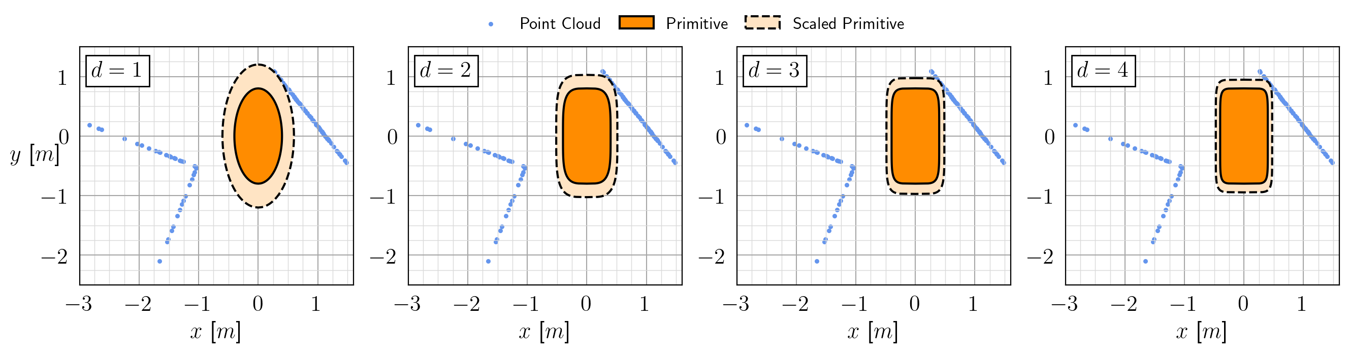
Figure 1: Visualization of the proposed point cloud CBF in a 2D scenario for different versions of higher-order ellipsoids. The blue dots represent the measured point cloud. The dark orange higher-order ellipse represents the unscaled primitive defined in (5), and the light orange higher-order ellipse represents the primitive after it is scaled by the scaling factor. The order of the ellipse is given in the upper left corner.

Assume the robot, in its body frame, is encapsulated by an ellipsoid $\mathcal{E}$ defined as

$$\mathcal{E}=\Big{\{}\bm{p}\ \Big{|}\ \bm{p}^{\top}\bm{P}\bm{p}\leq 1\Big{\}}$$ (5)

and the matrix $\bm{P}$ given by

$$\bm{P}=\begin{bmatrix}1/a^{2}&0&0\\ 0&1/b^{2}&0\\ 0&0&1/c^{2}\end{bmatrix}.$$ (6)

with $a,b,c\in\mathbb{R}_{+}$ denoting the lengths of its semi-axes.

Remark 2.

We call this ellipsoid (including the higher-order ellipsoids as defined in (10)) a Vessel that contains the robot.

Let the obstacles be given as a point cloud $\mathcal{P}\subset\mathbb{R}^{3}$ in the body frame of $\mathcal{E}$. Then, for each point $p_{j}\in\mathcal{P}$, we can compute the uniform scaling factor $\bm{s}_{j}\in\mathbb{R}_{+}$ between the ellipsoids and $\bm{p}_{j}$ as

$$\bm{s}_{j}^{2}=\bm{p}_{j}^{\top}\bm{P}\bm{p}_{j}.$$ (7)

As seen in Fig. 1, a larger-than-one scaling factor implies that the robot is not in collision with the point cloud. Thus, we can specify the safe set as the set of states where $\bm{s}_{j}^{2}\geq 1$. Define $\bm{\alpha}_{j}$ and $\bm{h}_{j}$ as

$$\bm{\alpha}_{j}=\bm{s}_{j}^{2},\quad\bm{h}_{j}=\bm{\alpha}_{j}-\bm{\beta}$$ (8)

where $\bm{\beta}\geq 1$. Then, the CBF between point cloud $\mathcal{P}$ and $\mathcal{E}$ can be computed as

$$\bm{h}=\min_{j}{\bm{h}_{j}}.$$ (9)

Remark 3.

From the derivations in [14], we know that by ensuring safety with respect to the point with the smallest CBF value, we can ensure safety with respect to all points in the point cloud.

A visualization of the effect of scaling an ellipsoid using the smallest scaling factor is given in Fig. 1. This formulation can be extended to higher-order ellipsoids defined as

$$\mathcal{E}^{\bm{d}}=\Big{\{}\bm{p}\Big{|}\bm{p}_{\bm{d}}(\bm{p},\bm{d})^{\top}\bm{P}^{\bm{d}}\bm{p}_{\bm{d}}(\bm{p},\bm{d})\leq 1\Big{\}}$$ (10)

with $\bm{d}\in\mathbb{N}$ representing the order of the ellipse and $\bm{p}_{\bm{d}}:\mathbb{R}^{3}\times\mathbb{N}\rightarrow\mathbb{R}^{n}$ defined as

$$\bm{p}_{\bm{d}}(\bm{p},\bm{d})=\begin{bmatrix}x^{\bm{d}}\\ y^{\bm{d}}\\ z^{\bm{d}}\end{bmatrix}\in\mathbb{R}^{3},\ \mathrm{with}\ \bm{p}=\begin{bmatrix}x\\ y\\ z\end{bmatrix}\in\mathbb{R}^{3}.$$ (11)

For higher-order ellipsoids, the scaling factor and CBF would be computed as

$$\bm{s}_{j} =\sqrt[\bm{d}]{\bm{p}_{\bm{d}}(\bm{p}_{j},\bm{d})^{\top}\bm{P}_{i}^{\bm{d}}\bm{p}_{\bm{d}}(\bm{p}_{j},\bm{d})}$$ (12a)

$$\bm{\alpha}_{j} =\bm{s}_{j}^{\bm{d}}$$ (12b)

$$\bm{h}_{j} =\bm{\alpha}_{j}-\bm{\beta}.$$ (12c)

Remark 4.

In this paper, ellipsoids refer to a higher-order ellipsoid of order one. The order for higher-order ellipsoids with $\bm{d}>1$ will be specified.

A visualization of using different orders of higher-order ellipsoids is also given in Fig. 1. Given that the minimum function is not differentiable, we follow the formulation in [8] and adopt a soft version, i.e., the $\mathrm{softmin}$ function, which is defined as

$$\operatorname*{softmin}_{j}\bm{h}_{j}=-\delta\ln\Bigg{(}\frac{1}{N}\sum_{j=1}^{N}{e^{-\bm{h}_{j}/\delta}}\Bigg{)}$$ (13)

where $N\in\mathbb{N}$ represents the number of points in the point cloud $\mathcal{P}$ and $\delta\in\mathbb{R}_{+}$. The value of $\mathrm{softmin}$ approximates the minimum function when $\delta$ is close to zero. The expression in (13) is susceptible to being subjected to numerical instability, which we address by adopting the following equivalent form [8]

$$\operatorname*{softmin}_{j}\bm{h}_{j} =\min_{j}\bm{h}_{j}+\operatorname*{softmin}_{j}\widehat{\bm{h}}_{j}$$ (14a)

$$\widehat{\bm{h}}_{j} =\bm{h}_{j}-\min_{k}\bm{h}_{k}.$$ (14b)

With this, the final form of our CBF formulation becomes

$$\bm{h}=\min_{j}\bm{h}_{j}-\delta\ln\Bigg{(}\frac{1}{N}\sum_{j=1}^{N}{e^{-\widehat{\bm{h}}_{j}/\delta}}\Bigg{)}.$$ (15)

The partial derivative of the CBF with respect to the position and orientation of the ellipsoid can be computed as

$$\frac{\partial\bm{h}}{\partial(\bm{r},\bm{q})}=\frac{\displaystyle\sum_{j=1}^{N}{\Bigg{[}e^{-\widehat{\bm{h}}_{j}/\delta}\frac{\partial\bm{h}_{j}}{\partial(\bm{r},\bm{q})}}\Bigg{]}}{\displaystyle\sum_{j=1}^{N}{e^{-\widehat{\bm{h}}_{j}/\delta}}}\in\mathbb{R}^{7}$$ (16)

where $\bm{r}\in\mathbb{R}^{3}$ and $\bm{q}\in\mathbb{H}$ ($\mathbb{H}$ represent the Hamiltonian) represents the position of and orientation as quaternions of $\mathcal{E}$ in the world frame, respectively. Next, we present the theoretical results that show the proposed point cloud CBF formulation in (15) is a valid CBF.

Theorem 1.

For a point cloud $\mathcal{P}$, the CBF proposed in (15) is continuously differentiable with respect to the position and orientation of its encapsulating higher-order ellipsoid.

Proof.

The proof utilizes the following properties: for two continuously differentiable functions $\bm{f}_{1}:\mathbb{R}^{n}\rightarrow\mathbb{R}$ and $\bm{f}_{2}:\mathbb{R}^{n}\rightarrow\mathbb{R}$, we have $\bm{f}_{1}(\bm{f}_{2}(\bm{x}))$, $\bm{f}_{1}(\bm{x})+\bm{f}_{2}(\bm{x})$, and $\bm{f}_{1}(\bm{x})\bm{f}_{2}(\bm{x})$ are all continuously differentiable functions. For a point $\bm{p}_{j}$ measured in the body frame of $\mathcal{E}$, its corresponding world frame coordinate is

$$\bm{p}_{w,j}=\bm{Rp_{j}+r}=\begin{bmatrix}x_{w,j}&y_{w,j}&z_{w,j}\end{bmatrix}^{\top}.$$ (17)

where $\bm{R}\in\mathrm{SO}(3)$ represents the orientation of $\mathcal{E}$ in the world frame as a rotation matrix. Then, expanding the CBF in (12c) for an order $\bm{d}$ ellipsoid yields

$$\bm{h}_{j}= \ \frac{1}{a^{2\bm{d}}}\Big{[}-(\bm{r}_{x}-x_{w,j})(2\bm{q}_{w}^{2}+2\bm{q}_{x}^{2}-1)$$

$$-\ 2(\bm{r}_{y}-y_{w,j})(\bm{q}_{w}\bm{q}_{z}+\bm{q}_{x}\bm{q}_{y})$$

$$+\ 2(\bm{r}_{z}-z_{w,j})(\bm{q}_{w}\bm{q}_{y}-\bm{q}_{x}\bm{q}_{z})\Big{]}^{2\bm{d}}$$

$$+\ \frac{1}{b^{2\bm{d}}}\Big{[}2(\bm{r}_{x}-x_{w,j})(\bm{q}_{w}\bm{q}_{z}-\bm{q}_{x}\bm{q}_{y})$$

$$-\ (\bm{r}_{y}-y_{w,j})(2\bm{q}_{w}^{2}+2\bm{q}_{y}^{2}-1)$$

$$-\ 2(\bm{r}_{z}-z_{w,j})(\bm{q}_{w}\bm{q}_{x}+\bm{q}_{y}\bm{q}_{z})\Big{]}^{2\bm{d}}$$

$$+\ \frac{1}{c^{2\bm{d}}}\Big{[}-2(\bm{r}_{x}-x_{w,j})(\bm{q}_{w}\bm{q}_{y}+\bm{q}_{x}\bm{q}_{z})$$

$$+\ 2(\bm{r}_{y}-y_{w,j})(\bm{q}_{w}\bm{q}_{x}+\bm{q}_{y}\bm{q}_{z})$$

$$-\ (\bm{r}_{z}-z_{w,j})(2\bm{q}_{w}^{2}+2\bm{q}_{z}^{2}-1)\Big{]}^{2\bm{d}}-\bm{\beta}.$$ (18)

Then, based on the aforementioned properties, we can see that $\bm{h}_{j}$ is continuously differentiable, with respect to $\bm{r}=[\bm{r}_{x},\bm{r}_{y},\bm{r}_{z}]$ and $\bm{q}=[\bm{q}_{w},\bm{q}_{x},\bm{q}_{y},\bm{q}_{z}]$. ∎

Remark 5.

The proposed point cloud CBF formulation is for velocity control, i.e., systems with the dynamics $\dot{\bm{x}}=\bm{u}$. Thus, $\bm{u}=\mathbf{0}$ is always a feasible solution to the CBFQP within the safe set $\mathcal{C}$.

Remark 6.

Apart from degenerate cases where the point cloud fully surrounds the robot, there always exists a control input that enables the robot to move away from the obstacles, which means that $\partial\bm{h}/\partial\bm{x}\neq 0$ for all $\bm{x}\in\partial\mathcal{C}$.

Theorem 2.

For systems with dynamics $\dot{\bm{x}}=\bm{u}$, the CBF formulation in (15) is a valid CBF.

Proof.

The proof directly follows from Theorem 1, Remark 5, and Remark 6. ∎

IV-B Mariner: CBF-Based Safe Preview Control

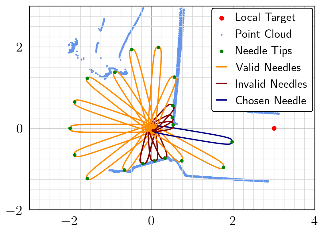
Figure 2: Visualization of the proposed preview control method in a 2D scenario with higher-order ellipsoids with order four.

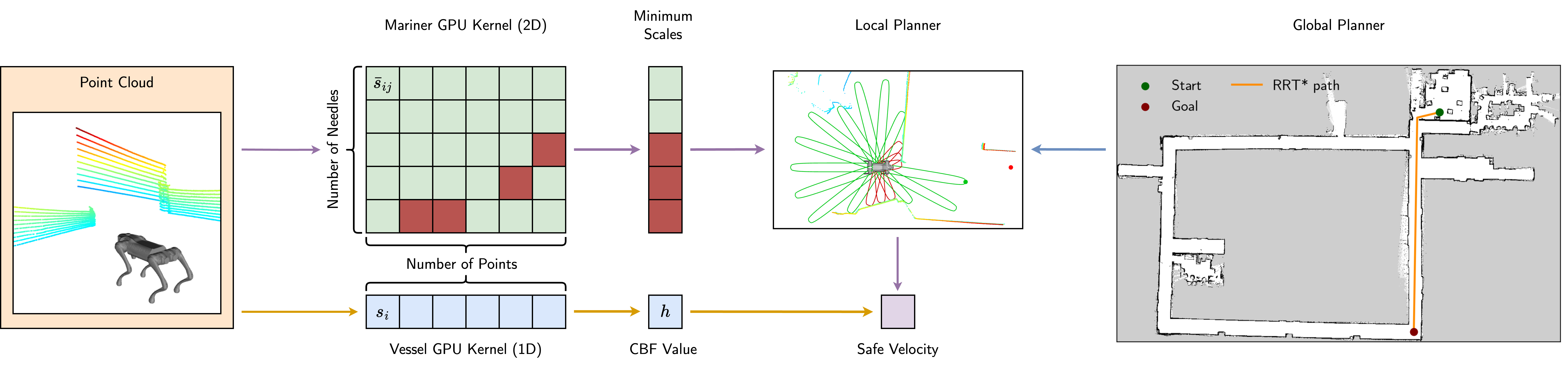
Figure 3: Illustration of the complete motion planning pipeline. The values along the orange arrows are updated at 10 $\mathrm{H}\mathrm{z}$ (LiDAR update frequency), the purple arrows are updated at 2 $\mathrm{H}\mathrm{z}$, and the blue arrows are updated only once at the beginning of our experiments.

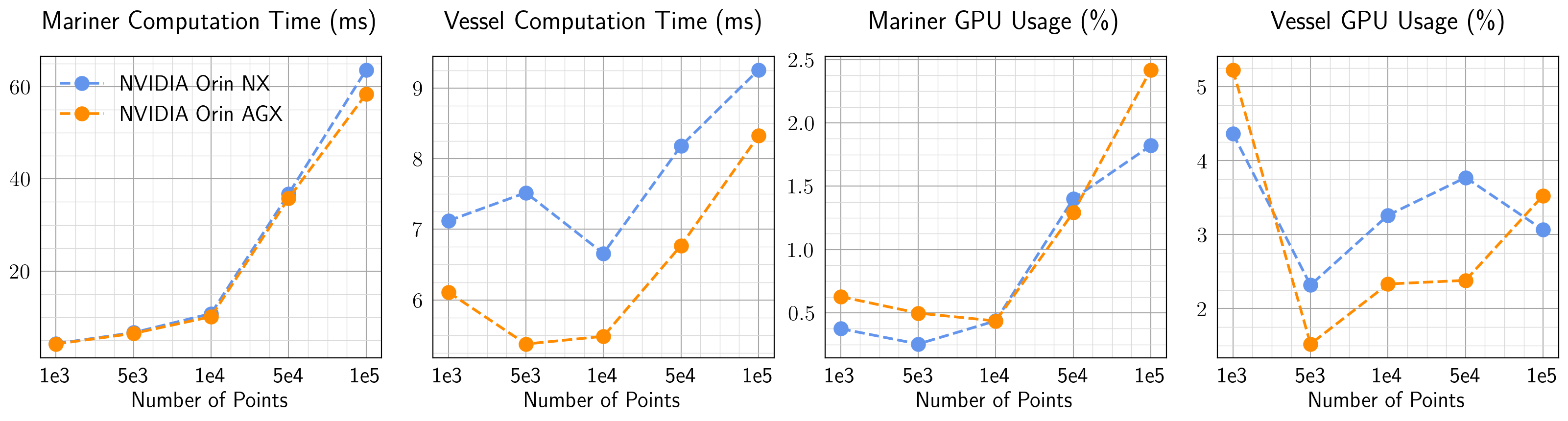
Figure 4: Comparison of the proposed algorithm’s computation time and GPU usage on different computers. The GPU usage is computed when running the Mariner at 2 $\mathrm{H}\mathrm{z}$ and the Vessel at 10 $\mathrm{H}\mathrm{z}$.

For CBFQP-based methods, one undesirable scenario is when the solution to (4) is $\bm{u}=0$. When such a scenario occurs, we say that the robotic system has fallen into an undesired equilibrium state [8]. Since the proposed CBF in Section IV-A is for velocity control, $\bm{u}=0$ means that the commanded velocity is zero and the robot is stuck at its current position. One way to avoid this issue is to use an MPC-based approach with a sufficiently long preview horizon. However, incorporating the current CBF formulation with an MPC-based approach is computationally expensive and generally creates a nonlinear and nonconvex numerical optimization problem. Therefore, we propose a novel preview controller that, by fixing the shape of the future path, transforms the preview motion planning problem into a collision-free inverse kinematics problem.

The simplification of the motion planning problem by using a fixed set of paths has been studied in dynamic window based approaches [19]. However, in [19], the paths are generated using a fixed velocity profile, which is less flexible than desired. In this work, we propose Mariner, a point cloud CBF based local planner that represents the paths in the configuration space and exploits GPU acceleration to check hundreds of paths (which are referred to as needles) in a few milliseconds. Mathematically, for the $i$-th needle, it is represented using a higher-order ellipsoid defined as

$$\frac{(x-\bar{\bm{s}}_{i}\bar{a}_{i})^{\bar{\bm{d}}}}{\bar{\bm{s}}_{i}^{\bar{\bm{d}}}\bar{a}_{i}^{\bar{\bm{d}}}}+\frac{y^{\bar{\bm{d}}}}{\bar{b}_{i}^{\bar{\bm{d}}}}+\frac{z^{\bar{\bm{d}}}}{\bar{c}_{i}^{\bar{\bm{d}}}}=1$$ (19)

where $\bar{a}_{i},\bar{b}_{i},\bar{c}_{i}\in\mathbb{R}$ represents the length of the semi-axes of the unscaled needle, $\bar{\bm{d}}\in\mathbb{N}$ represents the ellipsoid order used to represent the needle, and $\bar{\bm{s}}_{i}\in\mathbb{R}$ is the scaling factor of the needle. As shown in Fig. 2, the configuration space is discretized using $n_{\text{needle}}\in\mathbb{N}$ needles. Each needle is chosen to point towards a fixed angle within the robot’s body frame obtained from a distribution function $\mathrm{dist}:\mathbb{N}\rightarrow\mathbb{R}$ that maps the needle index to its corresponding angle. For example, in Fig. 2, $n_{\text{needle}}=19$ and

$$\mathrm{dist}(i)=\theta_{\text{needle},i}=\frac{2\pi}{n_{\text{needle}}}i-\pi.$$ (20)

Note that, unlike the Vessel, only the length is extended when the needles are scaled. For each needle, its body frame is located at the robot center with its $z$ axis pointing upwards and its $x$ axis pointing from the robot center to the tip of the needle. To compute the scaling factor $\bar{\bm{s}}_{i}$, we first rotate the point cloud by the needle angle to get the points within the needle’s body frame

$$\bm{p}_{j}=\begin{bmatrix}x_{j}&y_{j}&z_{j}\end{bmatrix}^{\top}=\mathbf{R}(\theta_{\text{needle},i})^{\top}\bm{p}_{w,j}$$ (21)

with $\theta_{\text{needle},i}\in\mathbb{R}$ represents the angle the $i$-th needle is pointing towards, $\mathbf{R}(\theta_{\text{needle},i})\in\mathrm{SO(3)}$ represents the rotation matrix corresponding to the $i$-th needle angle, and $\bm{p}_{j},\bm{p}_{w,j}\in\mathbb{R}^{3}$ representing the position of the $j$-th point in the needle’s body frame and world frame, respectively, For $\bm{p}_{j}$, define

$$m_{ij}^{\bar{\bm{d}}}=1-\frac{y_{j}^{\bar{\bm{d}}}}{\bar{b}_{i}^{\bar{\bm{d}}}}+\frac{z_{j}^{\bar{\bm{d}}}}{\bar{c}_{i}^{\bar{\bm{d}}}}.$$ (22)

Since the needle can only change its length, not its width or height, we only compute the scale against points with $m_{ij}^{\bar{\bm{d}}}>0$. With this assumption, we have the scale of the $i$-th needle with respect to the $j$-th point as

$$\bar{\bm{s}}_{ij}=\frac{x_{j}}{(1+m_{ij})\bar{a}_{i}}.$$ (23)

For each needle, we compute the scale with respect to all valid points. Then, we choose the minimum value among all of the scales as the scale of the needle, and the scale is set to be a predefined $\bar{\bm{s}}_{\max}$ if there are no valid points or if $\bar{\bm{s}}_{i}>\bar{\bm{s}}_{\max}$, i.e.,

$$\bar{\bm{s}}_{i}=\begin{cases}\displaystyle\bar{\bm{s}}_{\max}&\displaystyle\text{if }\min_{j}{\bar{\bm{s}}_{ij}}>\bar{\bm{s}}_{\max}\text{ or no valid points}\\ \displaystyle\min_{j}{\bar{\bm{s}}_{ij}}&\displaystyle\text{if }\min_{j}{\bar{\bm{s}}_{ij}}\leq\bar{\bm{s}}_{\max}.\end{cases}$$ (24)

Then, we check the size of the needle scales and only consider needles with $\bar{\bm{s}}_{i}\geq\bar{\bm{s}}_{\min}$ as valid needles (orange needles shown in Fig. 2) and treat the rest as invalid needles (red needles shown in Fig. 2). For all valid needles, we compute the distance between the scaled needle’s tip (green dots in Fig. 2) and the target $\bm{p}^{\star}\in\mathbb{R}^{3}$ (red dot in Fig. 2). Finally, we choose the needle with its scaled tip closest to the target as the chosen needle (blue needle in Fig. 2) and its scaled tip as the preview control target. The pseudo-code of this process is given in Algorithm 1.

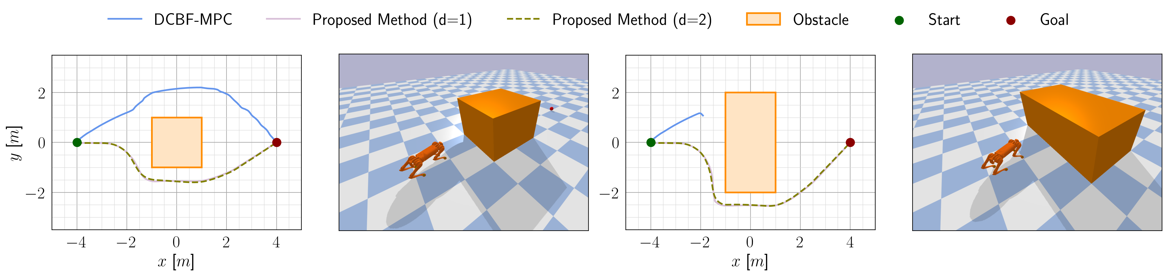
Figure 5: Illustration of the comparison studies between our proposed method and DCBF-MPC [1]. The first and third plots from the left show a top-down view of the generated trajectories. The green dot represents the starting position, the red dot represents the goal position, the orange block represents the obstacle, the trajectories of our proposed method are the light purple and dark green curves (they almost overlap), and the trajectory generated DCBF-MPC is the blue curve. The corresponding simulation scenarios are shown in the second and fourth images from the left.

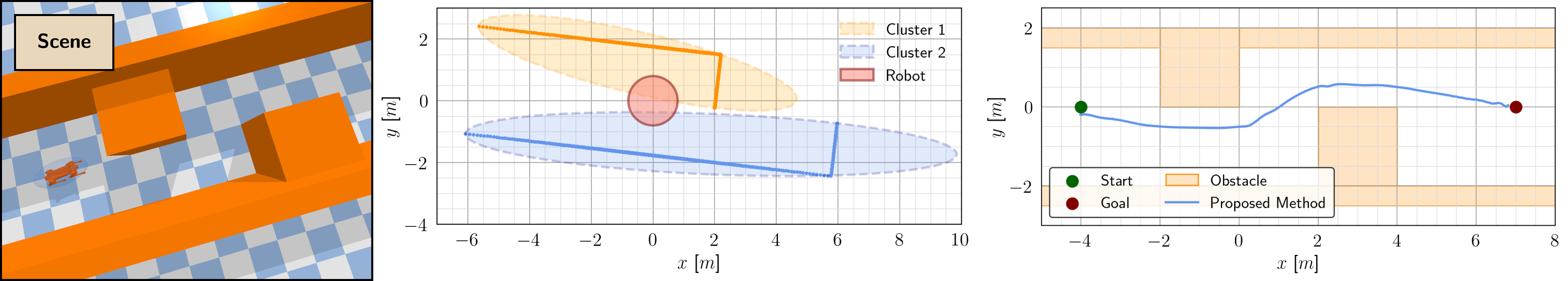
Figure 6: Comparison between our method and DCBF-MPC in a hallway. The left figure shows a top-down view of the simulated scene. The middle figure shows the positions of the MVEE-generated ellipsoids relative to the robot. The right figure shows the path generated by our proposed method. It can be seen that DCBF-MPC fails to find a solution due to starting in an invalid state, while our approach successfully plans a collision-free path.

IV-C Complete Pipeline

Algorithm 1 Mariner: CBF-based Safe Preview Control

1:Get point cloud data $\mathcal{P}$, number of needles $n_{\text{needle}}$, a distribution function $\mathrm{dist}$, and current global planner target $\bm{p}^{\star}$;

2:for $i=0\ \text{to}\ n_{\text{needle}}-1$ do

3:     $\theta_{\text{needle},i}=\mathrm{dist}(i)$;

4:     Transform and filter $\mathcal{P}$ based on (21) and (22);

5:     Compute the scale of this needle $\bar{\bm{s}}_{i}$;

6:Find the scaled needle with its tip closest to $\bm{p}^{\star}$;

7:Set the preview control target to be the tip of the chosen needle from the last step;

The complete navigation pipeline includes the global planner, the Mariner, and the Vessel. When given a map of the environment, the global planner creates waypoints $\{\bm{p}_{k}^{\star}\}_{k=1,\cdots,n_{k}}\subset\mathbb{R}^{3}$ between the current position of the robot and the target position, with $n_{k}\in\mathbb{N}$ being the number of waypoints. As mentioned in Section III, the map does not need to include transient structures. Then, the Mariner determines the local target ${}^{\mathcal{B}}\bm{p}_{\text{target}}^{\star}$. Finally, a performance controller is used to command the robot toward the local target, and the Vessel filters the performance controller command to ensure safety. Note that any sampling-based [20] or search-based motion planning algorithm can be deployed for the global planner. For details regarding examples of the global planners that could be deployed, please refer to Section V. The complete pipeline is also illustrated in Fig. 3.

V Experiments

In this section, we show the effectiveness of our proposed method by comparing our proposed point-cloud CBF with existing point cloud based CBF formulations and validating its performance in real-world settings.

V-A Setup

We validate our algorithm using a Unitree B1 and Go2 robot. The simulated experiments are performed in Pybullet with a Unitree B1. All computations for real-world experiments are performed onboard using an NVIDIA Jetson Orin NX for the Unitree Go2 and a Jetson Orin AGX for the Unitree B1. Both robots obtain the point clouds using a 16-channel 3D LiDAR at 10 $\mathrm{H}\mathrm{z}$. In the remainder of this section, the CBFQP models the dynamics of the quadruped system as a single integrator with orientation, i.e.,

$$\dot{\bm{x}}=\bm{u}=\begin{bmatrix}\bm{v}^{\top}&\bm{\omega}\end{bmatrix}^{\top}\in\mathbb{R}^{4}$$ (25)

with $\bm{v}\in\mathbb{R}^{3}$ and $\bm{\omega}\in\mathbb{R}$ being the linear and angular velocity, respectively. The performance controller has the form of

$$\bm{u}_{\mathrm{ref}} =\begin{bmatrix}\bm{v}^{\top}&\bm{\omega}\end{bmatrix}^{\top}\in\mathbb{R}^{4}$$ (26a)

$$\bm{v} =\bm{K}_{v}({}^{\mathcal{B}}\bm{p}_{\text{target}}^{\star}-{}^{\mathcal{B}}\bm{p}_{\text{robot}})$$ (26b)

$$\bm{\omega} =\bm{K}_{\omega}({}^{\mathcal{B}}\bm{\phi}_{\text{target}}-{}^{\mathcal{B}}\bm{\phi}_{\text{robot}})$$ (26c)

with $\bm{K}_{v}\in\mathbb{R}_{\succ 0}^{3\times 3}$ and $\bm{K}_{\omega}\in\mathbb{R}_{+}$ representing the gain matrices, ${}^{\mathcal{B}}\bm{\phi}_{\text{target}}\in\mathbb{R}$ the desired yaw angle which points towards the target, ${}^{\mathcal{B}}\bm{p}_{\text{robot}}\in\mathbb{R}^{3}$ the robot position in its body frame (is constantly zero), and ${}^{\mathcal{B}}\bm{\phi}_{\text{robot}}\in\mathbb{R}$ the robot yaw angle measured in its body frame (also is constantly zero). For the CBFQP, we choose

$$\Gamma(\bm{h}(\bm{x}))=\bar{\gamma}\bm{h}(\bm{x})$$ (27)

where $\bar{\gamma}\in\mathbb{R}_{+}$. We use an NMPC [21] controller to transform the commanded linear and angular velocity to joint torques in the simulation studies. In the experimental studies we use the onboard proprietary controller to track the commanded linear and angular velocity. For real-world experiments, the SLAM toolbox [22] is used for mapping and localization. To reduce the computation time of the point cloud based CBF, we created custom CUDA kernels using NVIDIA Warp [23] to parallelize the computations. For the Vessel, we create a 1D kernel, and a 2D kernel is used for the Mariner. We show the computation time for an NVIDIA Jetson Orin NX and NVIDIA Jetson Orin AGX in Fig. 4. In all the cases shown in Fig. 4, we set $n_{\mathrm{needle}}=100$. Additional experimental results, including the real-world experiments using Unitree B1, can be found in the accompanying video: https://youtu.be/lDmayeYcu28.

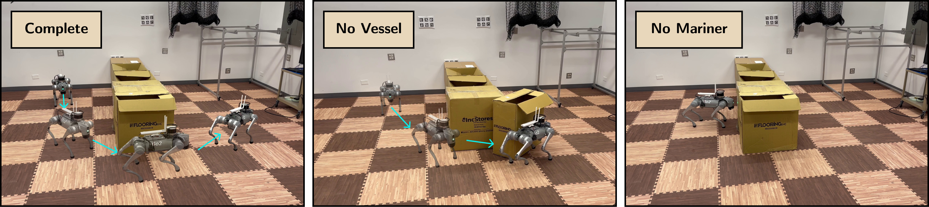
Figure 7: The experimental setting and ablation study results for showing the effectiveness of each component of the local planner where “Complete” refers to having both the Mariner and Vessel, “No Vessel” refers to only using the Mariner, and “No Mariner” refers to only using the Vessel.

V-B Simulation Studies

We compare our approach with a recent point cloud CBF based method introduced in [1] (DCBF-MPC), where the point cloud is first clustered and then encapsulated using minimum-volume enclosing ellipsoids (MVEE) [24]. Furthermore, [1] models the robot with a sphere, which leads to more conservatism. We compare the performance where the task of interest is navigating to a goal location while avoiding collision with obstacles. The simulation settings are shown in Fig. 5 and Fig. 6. In all settings, the Vessel is in the form of higher-order ellipsoids of order one with semi-axes $(a,b,c)=(0.8,0.4,0.4)~{}$\mathrm{m}$$. The Mariner uses needles that are uniformly distributed with their semi-axes being $(\bar{a},\bar{b},\bar{c})=(2,0.8,0.8)~{}$\mathrm{m}$$, $\bar{\bm{d}}=2$, $n_{\mathrm{needle}}=100$, and uses the same distribution function as in (20).

For our implementation of the approach in [1], we set the integration time step to be 0.5 $\mathrm{s}$, the preview length to be 30 time steps (15 seconds), the safe distance $d_{\mathrm{safe}}=0.8$, $\gamma=0.3$, and use DBSCAN [25] for clustering. The NMPC is solved using CasADi [26]. It can be seen that the approach in [1] can solve the left scenario in Fig. 5 where the obstacle is smaller. However, for larger obstacles, i.e., the right scenario, the quadruped gets stuck in front of the obstacle. This is likely caused by getting stuck in a suboptimal local minimum for the NMPC solver. Moreover, the NMPC scales poorly with respect to the length of the preview horizon, while our proposed preview controller scales constantly with respect to the length of the Mariner needles. The requirement for a point cloud preprocessing pipeline is another limitation of the DCBF-MPC approach. Specifically, the usage of MVEEs also makes the CBF formulation for DCBF-MPC much more conservative than our proposed approach, especially in cluttered scenes, e.g., hallways. For the scene shown in Fig. 6, the usage of MVEEs causes the robot to appear to be in a collision state while being sufficiently far away from the obstacles. This causes the NMPC to fail, given that the initial state is already invalid. These issues may be alleviated by adopting better point cloud preprocessing pipelines and introducing a backup controller, which is not required by our method. Another major claim of the DCBF-MPC approach is that it can handle dynamic obstacles. Although, for the simplicity of presentation, dynamic obstacles are not explicitly considered, given the computational efficiency of both the Vessel and Mariner, the capability to replan at sensor frame rate makes the proposed method responsive enough to react to dynamic obstacles, as shown in the accompanied video.

V-C Experimental Deployment

This section presents experimental results of deploying our algorithm on a Unitree Go2 robot. The goal is to reach a target location while avoiding collision with obstacles (the boxes in Fig. 7). The semi-axes $(a,b,c)$ for the Vessels are $(0.5,0.3,0.2)~{}$\mathrm{m}$$. The Needles are modeled using ellipsoids with semi-axes $(0.8,0.1,0.2)~{}$\mathrm{m}$$, $\bar{\bm{d}}=2$, $n_{\text{needle}}=100$, and the distribution function in (20). The generated trajectories are shown in Fig. 7. The robot successfully reaches the target position on the other side of the box wall when using both the Vessel and Mariner (denoted as complete in Fig. 7). The robot collides with the boxes if the Vessel is not activated. If the Mariner is not activated, the robot fails to escape from the equilibrium of the CBFQP controller. For results of our proposed pipeline on the Unitree B1 robot in a similar setting, please refer to the accompanying video. Next, we show the results of integrating our proposed local planner with a global planner. The RRT^⋆ implementation in OMPL [27] is used to generate a global plan, which is shown in Fig. 3. Then, random obstacles (four boxes as shown in Fig. 8) are added to the scene. Finally, following the pipeline shown in Section IV-C, the robot tracks the RRT-generated waypoints. The Mariner and Vessel settings are identical to the experiments in Section V-C. As shown in Fig. 8, the local planner generates collision-free paths for the robot without getting stuck at any point along the trajectory. Additional experiments are in the accompanying video. For the additional experiments, the obstacles were also not included when planning the global path.

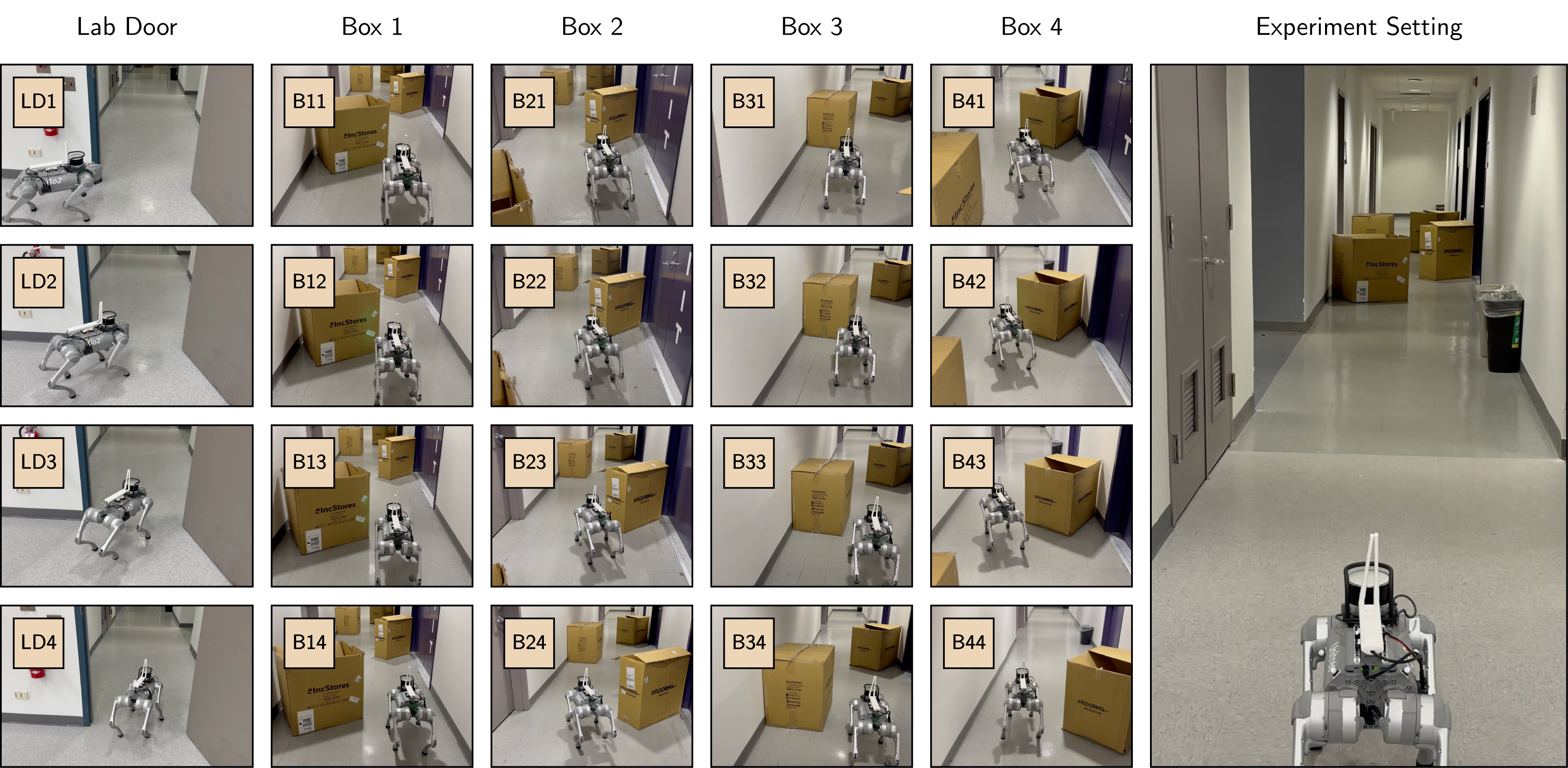
Figure 8: Result of our complete pipeline. There are five main obstacles in the illustrated settings. For each obstacle, four snapshots are provided to depict the motion generated by the proposed local planner.

VI Conclusion

In this work, we proposed Vessel a novel point cloud based CBF formulation and Mariner a novel local planner that can process point cloud data and move the CBF-based controller out of local equilibriums. We have shown theoretically that the proposed CBF formulation is a valid CBF. To show the effectiveness of our approach, we have tested it on quadrupedal robots in both simulation and the real world, along with the proposed motion planning pipeline.

VII Acknowledgement

We would like to thank Tanishq Bhansali, Naren Devarakonda, Raktim Goswami, and Pranay Gupta for their assistance with the experiments.

References

- [1] Z. Jian, Z. Yan, X. Lei, Z. Lu, B. Lan, X. Wang, and B. Liang, “Dynamic control barrier function-based model predictive control to safety-critical obstacle-avoidance of mobile robot,” in Proceedings of the IEEE International Conference on Robotics and Automation, London, United Kingdom, May 2023, pp. 3679–3685.
- [2] H. U. Unlu, V. M. Gonçalves, D. Chaikalis, A. Tzes, and F. Khorrami, “A control barrier function-based motion planning scheme for a quadruped robot,” in Procceedings of IEEE International Conference on Robotics and Automation, Yokohama, Japan, May 2024, (To appear).
- [3] B. Dai, P. Krishnamurthy, A. Papanicolaou, and F. Khorrami, “State constrained stochastic optimal control for continuous and hybrid dynamical systems using DFBSDE,” Automatica, vol. 155, p. 111146, 2023.
- [4] J. B. Rawlings, D. Q. Mayne, and M. Diehl, Model predictive control: theory, computation, and design. Nob Hill Publishing, Madison, WI, 2017, vol. 2.
- [5] B. Dai, P. Krishnamurthy, A. Papanicolaou, and F. Khorrami, “State constrained stochastic optimal control using LSTMs,” in Proceedings of the American Control Conference, New Orleans, LA, May 2021, pp. 1294–1299.
- [6] S. Wei, P. Krishnamurthy, and F. Khorrami, “Confidence-aware safe and stable control of control-affine systems,” CoRR, vol. abs/2403.09067, 2024.
- [7] A. D. Ames, S. Coogan, M. Egerstedt, G. Notomista, K. Sreenath, and P. Tabuada, “Control barrier functions: Theory and applications,” in Proceedings of the European Control Conference, Naples, Italy, June 2019, pp. 3420–3431.
- [8] V. M. Gonçalves, P. Krishnamurthy, A. Tzes, and F. Khorrami, “Using circulation to mitigate spurious equilibria in control barrier function,” in Proceedings of the IEEE Conference on Decision and Control, Singapore, Singapore, December 2023, pp. 1770–1775.
- [9] A. Thirugnanam, J. Zeng, and K. Sreenath, “Safety-critical control and planning for obstacle avoidance between polytopes with control barrier functions,” in Proceedings of International Conference on Robotics and Automation, Philadelphia, PA, May 2022, pp. 286–292.
- [10] J. Zeng, B. Zhang, and K. Sreenath, “Safety-critical model predictive control with discrete-time control barrier function,” in Proceedings of the American Control Conference, New Orleans, LA, May 2021, pp. 3882–3889.
- [11] B. Dai, P. Krishnamurthy, and F. Khorrami, “Learning a better control barrier function,” in Proceedings of the IEEE Conference on Decision and Control, Cancún, Mexico, December 2022, pp. 945–950.
- [12] B. Dai, H. Huang, P. Krishnamurthy, and F. Khorrami, “Data-efficient control barrier function refinement,” in Proceedings of the American Control Conference, San Diego, CA, May 2023, pp. 3675–3680.
- [13] B. Dai, R. Khorrambakht, P. Krishnamurthy, V. Gonçalves, A. Tzes, and F. Khorrami, “Safe navigation and obstacle avoidance using differentiable optimization based control barrier functions,” IEEE Robotics and Automation Letters, vol. 8, no. 9, pp. 5376–5383, 2023.
- [14] B. Dai, R. Khorrambakht, P. Krishnamurthy, and F. Khorrami, “Differentiable optimization based time-varying control barrier functions for dynamic obstacle avoidance,” CoRR, vol. abs/2309.17226, 2023.
- [15] S. Wei, B. Dai, R. Khorrambakht, P. Krishnamurthy, and F. Khorrami, “Diffocclusion: Differentiable optimization based control barrier functions for occlusion-free visual servoing,” IEEE Robotics and Automation Letters, vol. 9, no. 4, pp. 3235–3242, 2024.
- [16] C. J. Ong and E. G. Gilbert, “Growth distances: new measures for object separation and penetration,” IEEE Transactions on Robotics and Automation, vol. 12, no. 6, pp. 888–903, 1996.
- [17] E. G. Gilbert and C. J. Ong, “New distances for the separation and penetration of objects,” in Proceedings of the IEEE International Conference on Robotics and Automation, San Diego, CA, May 1994, pp. 579–586.
- [18] K. Tracy, T. A. Howell, and Z. Manchester, “Differentiable collision detection for a set of convex primitives,” in Proceedings of the IEEE International Conference on Robotics and Automation, London, United Kingdom, May 2023, pp. 3663–3670.
- [19] D. Fox, W. Burgard, and S. Thrun, “Controlling synchro-drive robots with the dynamic window approach to collision avoidance,” in Proceedings of the IEEE/RSJ International Conference on Intelligent Robots and Systems, Osaka, Japan, November 1996, pp. 1280–1287.
- [20] S. Karaman and E. Frazzoli, “Sampling-based algorithms for optimal motion planning,” International Journal of Robotics Research, vol. 30, no. 7, pp. 846–894, 2011.
- [21] A. Meduri, P. Shah, J. Viereck, M. Khadiv, I. Havoutis, and L. Righetti, “Biconmp: A nonlinear model predictive control framework for whole body motion planning,” IEEE Transactions on Robotics, vol. 39, no. 2, pp. 905–922, 2023.
- [22] S. Macenski and I. Jambrecic, “SLAM toolbox: SLAM for the dynamic world,” Journal of Open Source Software, vol. 6, no. 61, p. 2783, 2021.
- [23] M. Macklin, “Warp: A high-performance Python framework for GPU simulation and graphics,” March 2022, NVIDIA GPU Technology Conference.
- [24] L. G. Khachiyan, “A polynomial algorithm in linear programming,” Doklady Akademii Nauk, vol. 244, no. 5, pp. 1093–1096, 1979.
- [25] M. Ester, H. Kriegel, J. Sander, and X. Xu, “A density-based algorithm for discovering clusters in large spatial databases with noise,” in Proceedings of the Second International Conference on Knowledge Discovery and Data Mining, Portland, OR, August 1996, pp. 226–231.
- [26] J. A. E. Andersson, J. Gillis, G. Horn, J. B. Rawlings, and M. Diehl, “Casadi: a software framework for nonlinear optimization and optimal control,” Mathematical Programming Computation, vol. 11, no. 1, pp. 1–36, 2019.
- [27] I. A. Sucan, M. Moll, and L. E. Kavraki, “The open motion planning library,” IEEE Robotics & Automation Magazine, vol. 19, no. 4, pp. 72–82, 2012.