Fault-tolerant properties of scale-free linear protocols for synchronization of homogeneous multi-agent systems

Abstract

Originally, protocols were designed for multi-agent systems (MAS) using information about the network. However, in many cases there is no or only limited information available about the network. Recently, there has been a focus on scale-free synchronization of multi-agent systems (MAS). In this case, the protocol is designed without any prior information about the network. As long as the network contains a directed spanning tree, the scale-free protocol guarantees that the network achieves synchronization.

If there is no directed spanning tree for the network then synchronization cannot be achieved. But what happens when these scale-free protocols are applied to such a network where the directed spanning tree no longer exists? The latter might arise if, for instance, a fault occurs in one of more crucial links. This paper establishes that the network decomposes into a number of basic bicomponents which achieves synchronization among all nodes in this basic bicomponent. On the other hand, nodes which are not part of any basic bicomponent converge to a weighted average of the synchronized trajectories of the basic bicomponents. The weights are independent of the initial conditions and are independent of the designed protocol.

1 Introduction

The synchronization problem for multi-agent systems (MAS) has attracted substantial attention due to its potential for applications in several areas, see for instance the books [1, 2, 4, 8, 11, 12, 18] or the papers [5, 9, 10].

Most of the proposed protocols in the literature for synchronization of MAS require some knowledge of the communication network such as bounds on the spectrum of the associated Laplacian matrix or the number of agents. As it is pointed out in [14, 15, 16, 17], these protocols suffer from scale fragility where stability properties are lost when the size of the network increases or when the network changes due to addition or removal of links.

In the past few years, scale-free linear protocol design has been actively studied in the MAS literature to deal with the existing scale fragility in MAS [6]. The “scale-free” design implies that the protocols are designed solely based on the knowledge of agent models and do not depend on

• information about the communication network such as the spectrum of the associated Laplacian matrix or

• knowledge of the number of agents.

In, for instance, [6], scale-free protocols have been designed utilizing localized information exchange between agent and its neighbor for various cases of MAS problems. Due to this local information exchange the protocols are referred to as collaborative protocols.

By contrast, scale-free non-collaborative protocol designs only use relative measurements and no additional information exchange is allowed and therefore the protocols are fully distributed. The necessary and sufficient condition for solvability of scale-free design via non-collaborative linear protocol for MAS consisting of SISO agent model was recently reported, see [7].

For both collaborative and non-collaborative protocol, the designs achieve synchronization for any communication network which contains a directed spanning tree. If, for instance, due to a faulty link, the network no longer contains a directed spanning tree then synchronization is no longer achieved. This in itself is not surprising since the existence of a directed spanning tree is a necessary condition for achieving network synchronization.

However, it is an interesting question what happens if we apply our scale-free protocol to a network which no longer contains a directed spanning tree. Can this cause instability where synchronization errors blow up or is there some inherent stability in the system. This question is answered in this paper for both collaborative and non-collaborative scale-free protocols. We will establish that the network can be decomposed in basic bicomponents and a set of additional nodes.

• Within each basic bicomponent we achieve synchronization.

• The additional nodes converge to a weighted average of the synchronized trajectories of the basic bicomponents. The nonnegative weights are independent of the initial conditions, sum up to $1$ and are independent of the designed protocol.

It will be established that this behavior is true for both collaborative and non-collaborative protocols independent of their specific design methodology. This specific behavior will be referred to as cluster synchronization.

2 Communication network and graph

To describe the information flow among the agents we associate a weighted graph $\mathcal{G}$ to the communication network. The weighted graph $\mathcal{G}$ is defined by a triple $(\mathcal{V},\mathcal{E},\mathcal{A})$ where $\mathcal{V}=\{1,\ldots,N\}$ is a node set, $\mathcal{E}$ is a set of pairs of nodes indicating connections among nodes, and $\mathcal{A}=[a_{ij}]\in\mathbb{R}^{N\times N}$ is the weighted adjacency matrix with non negative elements $a_{ij}$. Each pair in $\mathcal{E}$ is called an edge, where $a_{ij}>0$ denotes an edge $(j,i)\in\mathcal{E}$ from node $j$ to node $i$ with weight $a_{ij}$. Moreover, $a_{ij}=0$ if there is no edge from node $j$ to node $i$. We assume there are no self-loops, i.e. we have $a_{ii}=0$. A path from node $i_{1}$ to $i_{k}$ is a sequence of nodes $\{i_{1},\ldots,i_{k}\}$ such that $(i_{j},i_{j+1})\in\mathcal{E}$ for $j=1,\ldots,k-1$. A directed tree is a subgraph (subset of nodes and edges) in which every node has exactly one parent node except for one node, called the root, which has no parent node. A directed spanning tree is a subgraph which is a directed tree containing all the nodes of the original graph. If a directed spanning tree exists, the root has a directed path to every other node in the tree [3].

The weighted in-degree of a vertex $i$ is given by

$$d_{\text{in}}(i)=\sum_{j=1}^{N}\,a_{ij}.$$

For a weighted graph $\mathcal{G}$, the matrix $L=[\ell_{ij}]$ with

$$\ell_{ij}=\left\{\;\begin{array}[]{cl}\sum_{k=1}^{N}a_{ik},&i=j,\\ -a_{ij},&i\neq j,\end{array}\right.$$

is called the Laplacian matrix associated with the graph $\mathcal{G}$. The Laplacian matrix $L$ has all its eigenvalues in the closed right half plane and at least one eigenvalue at zero associated with right eigenvector 1 [3]. Moreover, if the graph contains a directed spanning tree, the Laplacian matrix $L$ has a single (simple) eigenvalue at the origin and all other eigenvalues are located in the open right-half complex plane [11].

A directed communication network is said to be strongly connected if it contains a directed path from every node to every other node in the graph. For a given graph $\mathcal{G}$ every maximal (by inclusion) strongly connected subgraph is called a bicomponent of the graph. A bicomponent without any incoming edges is called a basic bicomponent. Every graph has at least one basic bicomponent. Networks have one unique basic bicomponent if and only if the network contains a directed spanning tree. In general, every node in a network can be reached from at least one basic bicomponent, see [13, page 7]. In Fig. 1 a directed communication network with its bicomponents is shown. The network in this figure contains 6 bicomponents, 3 basic bicomponents (the blue ones) and 3 non-basic bicomponents (the yellow ones).

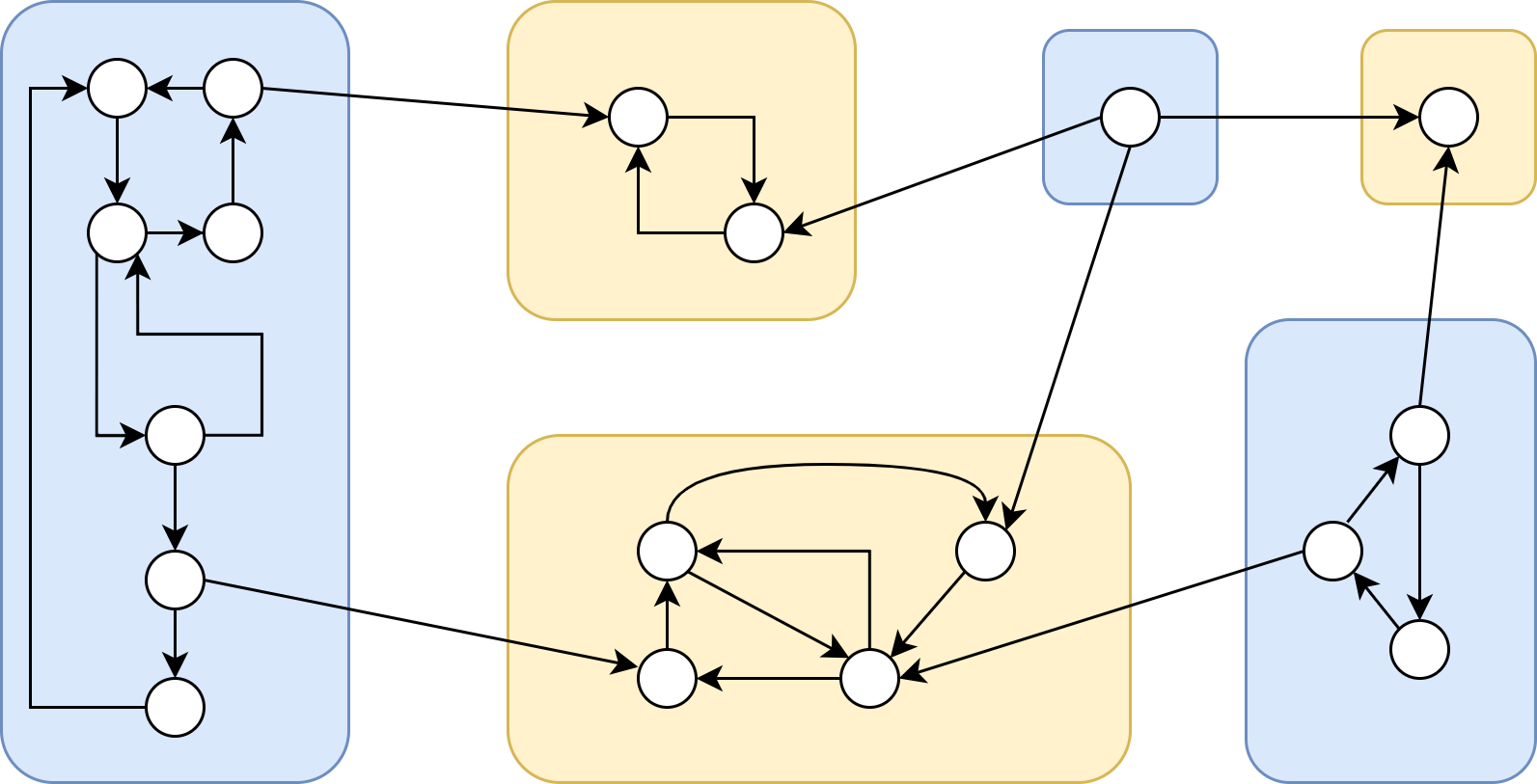
Figure 1: A directed communication network and its bicomponents.

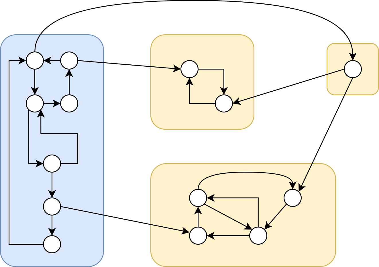
Figure 2: A directed communication network with a spanning tree and its bicomponents.

In the absence of a directed spanning tree, the Laplacian matrix of the graph has an eigenvalue at the origin with a mutiplicity $k$ larger than $1$. This implies that it is a $k$-reducible matrix and the graph has $k$ basic bicomponents. The book [18, Definition 2.19] shows that, after a suitable permutation of the nodes, a Laplacian matrix with $k$ basic bicomponents can be written in the following form:

$$L=\begin{pmatrix}L_{0}&L_{01}&\cdots&&L_{0k}\\ 0&L_{1}&0&\cdots&0\\ \vdots&\ddots&\ddots&\ddots&\vdots\\ \vdots&&\ddots&L_{k-1}&0\\ 0&\cdots&\cdots&0&L_{k}\end{pmatrix}$$ (1)

where $L_{1},\ldots,L_{k}$ are the Laplacian matrices associated to the $k$ basic bicomponents in our network. These matrices have a simple eigenvalue in $0$ because they are associated with a strongly connected component. On the other hand, $L_{0}$ contains all non-basic bicomponents and is a grounded Laplacian with all eigenvalues in the open right-half plane. After all, if $L_{0}$ would be singular then the network would have an additional basic bicomponent.

3 Scale-free non-collaborative protocol design for multi-agent systems

Consider multi-agent systems (MAS) consisting of $N$ identical agents:

$$\begin{array}[]{ccl}x_{i}^{+}(t)&=&Ax_{i}(t)+Bu_{i}(t),\\ y_{i}(t)&=&Cx_{i}(t),\end{array}$$ (2)

where $x_{i}(t)\in\mathbb{R}^{n}$, $y_{i}(t)\in\mathbb{R}$ and $u_{i}(t)\in\mathbb{R}$ are the state, output, and input of agent $i$, respectively, with $i=1,\ldots,N$. In the aforementioned presentation, for continuous-time systems, $x_{i}^{+}(t)=\dot{x}_{i}(t)$ with $t\in\mathbb{R}$ while for discrete-time systems, $x_{i}^{+}(t)=x_{i}(t+1)$ with $t\in\mathbb{Z}$.

For continuous time MAS, the communication network provides agent $i$ with the following information,

$$\zeta_{i}(t)=\sum_{j=1}^{N}a_{ij}(y_{i}(t)-y_{j}(t)),$$ (3)

where $a_{ij}>0$, and $a_{ii}=0$. The communication topology of the network can be described by a weighted and directed graph $\mathcal{G}$ with nodes corresponding to the agents in the network and the weight of edges given by coefficient $a_{ij}$. In terms of the coefficients of the associated Laplacian matrix $L$, $\zeta_{i}(t)$ can be rewritten as

$$\zeta_{i}(t)=\sum_{j=1}^{N}\ell_{ij}y_{j}(t).$$ (4)

For discrete-time agents, in particular, each agent $i\in\{1,\cdots,N\}$ has access to the quantity

$$\zeta_{i}(t)=\dfrac{1}{1+q_{i}}\sum_{j=1}^{N}a_{ij}(y_{i}(t)-y_{j}(t)),$$ (5)

where $q_{i}$ is an upper bound on $d_{\text{in}}(i)$ for $i,j\in\{1,\cdots,N\}$. In that case, we can use the modified information-exchange

$${\zeta}_{i}(t)=\sum_{j=1,j\neq i}^{N}d_{ij}(y_{i}(t)-y_{j}(t)),$$ (6)

instead of (4) where

$$d_{ij}=\frac{a_{ij}}{1+q_{i}},$$

for $i\neq j$ while

$$d_{ii}=1-\sum_{j=1,j\neq i}^{N}d_{ij}$$

Note that the weight matrix $D=[d_{ij}]$ is then a, so-called, row stochastic matrix. Let

$$Q_{\text{in}}=\operatorname{diag}\left(q_{1},q_{2},\cdots,q_{N}\right).$$

Then, the relationship between the row stochastic matrix $D$ and the Laplacian matrix $L$ is

$$(I+Q_{\text{in}})^{-1}L=I-D.$$ (7)

Non-collaborative protocols only use this relative measurement $\zeta_{i}$ and achieve fully distributed protocols. In scale-free protocols, we are looking for protocols which do not depend on the network structure. This is motivated by the fact that in many applications, an agent might be added/removed or a link might fail and you then do not want to have to redesign the protocols being used.

Definition 1

We denote by $\mathbb{G}^{N}$ the set of all directed graphs with $N$ nodes which contain a directed spanning tree.

We formulate the scale-free or scale-free synchronization problem of a MAS as follows.

Problem 1

The scale-free non-collaborative state synchronization problem for MAS (2) with communication given by (4) for continuous-time or (6) for discrete-time case is to find, if possible, a fixed linear protocol of the form:

$$\left\{\;\begin{array}[]{cl}x_{i,c}^{+}&=A_{c}x_{i,c}+B_{c}\zeta_{i},\\ u_{i}&=F_{c}x_{i,c}+G_{c}\zeta_{i},\end{array}\right.$$ (8)

where $x_{c,i}(t)\in\mathbb{R}^{n_{c}}$ is the state of protocol, such that state synchronization is achieved

$$\lim_{t\rightarrow\infty}x_{i}(t)-x_{j}(t)=0$$ (9)

for all $i,j=1,\ldots,N$ for any number of agents $N$, for any fixed communication graph $\mathcal{G}\in\mathbb{G}^{N}$ and for all initial conditions of agents and protocols.

We refer to a protocol (8) which solves Problem 1 as a scale-free non-collaborative linear protocol.

3.1 Continuous-time MAS

In this section, we focus on the continuous-time MAS. It is known that the Problem 1 is solvable for a large class of systems. We recall the following theorem which is provided in [7, Theorem 1].

Theorem 1

The scale-free continuous-time state synchronization problem as formulated in Problem 1 is solvable if the agent model (2) is either asymptotically stable or satisfies the following conditions:

• Stabilizable and detectable,

• Neutrally stable,

• Minimum phase,

• Uniform rank with the order of the infinite zero equal to one.

This paper wants to investigate what happens if we apply a protocol of the form (8) designed to solve Problem 1 to a network which does not contain a directed spanning tree.

By using protocol (8) we can define

$$\tilde{A}=\begin{pmatrix}A&BF_{c}\\ 0&A_{c}\end{pmatrix},\quad\tilde{B}=\begin{pmatrix}BG_{c}\\ B_{c}\end{pmatrix},\quad\tilde{C}=\begin{pmatrix}C&0\end{pmatrix}$$ (10)

We have the following result:

Theorem 2

Consider a continuous-time MAS with agent dynamics (2). Assume a protocol (8) solves the scale-free state synchronization problem.

If the network does not contain a directed spanning tree, then the Laplacian matrix of the graph has an eigenvalue at the origin with a mutiplicity $k$ larger than $1$. This implies that the graph has $k$ basic bicomponents. Then for any $i\in(1,\ldots,k)$,

• Within basic bicomponent $\mathcal{B}_{i}$, the state of the agents and the state of the associated protocol achieve synchronization and converge to trajectories $x_{i,s}$ and $x_{i,s,c}$ respectively satisfying

  $$\begin{pmatrix}\dot{x}_{i,s}\\ \dot{x}_{i,s,c}\end{pmatrix}=\tilde{A}\begin{pmatrix}x_{i,s}\\ x_{i,s,c}\end{pmatrix}$$

  whose initial condition is a linear combination of the initial conditions of the agents within this basic bicomponent.

• An agent $j$ which is not part of any of the basic bicomponents synchronizes to a trajectory:

  $$\sum_{i=1}^{k}\,\beta_{j,i}\begin{pmatrix}x_{i,s}\\ x_{i,s,c}\end{pmatrix}$$

  where the coefficients $\beta_{j,i}$ are nonnegative, satisfy:

  $$1=\sum_{i=1}^{k}\,\beta_{j,i}$$ (11)

  and only depend on the parameters of the network and do not depend on any of the initial conditions.

Proof: The paper [12, Chapter 2] has shown that we achieve scale-free state synchronization if and only if

$$\tilde{A}+\lambda\tilde{B}\tilde{C}$$ (12)

is asymptotically stable for all $\lambda\in\mathbb{C}$ with $\operatorname{Re}\lambda>0$. We use the decomposition (1) introduced before. We label the states of the agents and protocols as:

$$\bar{x}_{i}=\begin{pmatrix}x_{k_{i}+1}\\ x_{k_{i}+1,c}\\ x_{k_{i}+2}\\ x_{k_{i}+2,c}\\ \vdots\\ x_{k_{i+1}}\\ x_{k_{i+1},c}\end{pmatrix}$$

where $k_{0}=0$ and $k_{i+1}-k_{i}$ is the number of columns of $L_{i}$ for $i=0,\ldots,k$. It is easy to verify that the dynamics of the $i$’th basic bicomponent ($i\in\{1,\ldots,k\}$) is given by:

$$\dot{\bar{x}}_{i}=\left[(I\otimes\tilde{A})+L_{i}\otimes\tilde{B}\tilde{C}\right]\bar{x}_{i}$$

and since (12) is asymptotically stable for all $\lambda\in\mathbb{C}$ with $\operatorname{Re}\lambda>0$, classical results guarantee synchronization within this basic bicomponent and

$$\begin{pmatrix}x_{j}(t)\\ x_{j,c}(t)\end{pmatrix}-\begin{pmatrix}x_{i,s}(t)\\ x_{i,s,c}(t)\end{pmatrix}\rightarrow 0$$

as $t\rightarrow\infty$ for $j=k_{i}+1,\ldots,k_{i+1}$ with:

$$\begin{pmatrix}\dot{x}_{i,s}\\ \dot{x}_{i,s,c}\end{pmatrix}=\tilde{A}\begin{pmatrix}x_{i,s}\\ x_{i,s,c}\end{pmatrix}$$

and

$$\begin{pmatrix}x_{i,s}(0)\\ x_{i,s,c}(0)\end{pmatrix}=\sum_{i=k_{i}+1}^{k_{i+1}}\alpha_{i}\begin{pmatrix}x_{k_{i}+1}(0)\\ x_{k_{i}+1,c}(0)\end{pmatrix}$$

where

$$\bar{\alpha}_{i}=\begin{pmatrix}\alpha_{k_{i}+1}&\cdots&\alpha_{k_{i+1}}\end{pmatrix}$$

is the unique left-eigenvector associated with eigenvalue $0$ of $L_{i}$ whose elements are nonnegative and sum up to $1$. Define

$$\bar{x}_{0,s}=-\sum_{i=1}^{k}(L_{0}^{-1}L_{0,i}\textbf{1}_{i}\otimes I)\begin{pmatrix}x_{i,s}\\ x_{i,s,c}\end{pmatrix}$$

where $\textbf{1}_{i}$ is a column vector with all elements equal to $1$ whose size is equal to the number of columns of $L_{0,i}$ while $\textbf{1}_{0}$ is a column vector with all elements equal to $1$ whose size is equal to the number of columns of $L_{0}$. We claim that $\bar{x}_{0}(t)-\bar{x}_{0,s}(t)\rightarrow 0$ as $t\rightarrow\infty$ which implies that

$$\begin{pmatrix}x_{j}(t)\\ x_{j,c}(t)\end{pmatrix}-\sum_{i=1}^{k}\beta_{j,i}\begin{pmatrix}x_{i,s}(t)\\ x_{i,s,c}(t)\end{pmatrix}\rightarrow 0$$ (13)

as $t\rightarrow\infty$ for $j=1,\ldots,k_{1}$ where

$$\begin{pmatrix}\beta_{1,i}\\ \beta_{2,i}\\ \vdots\\ \beta_{k_{0},i}\end{pmatrix}=-L_{0}^{-1}L_{0,i}\textbf{1}_{i}$$ (14)

Note that the elements of $L_{0,i}$ are all nonpositive and the elements of $L_{0}^{-1}$ are all nonnegative (as the inverse of a grounded Laplacian matrix). This immediately shows that the coefficients $\beta_{j,i}$ are all nonnegative. Moreover,

$$L\begin{pmatrix}\textbf{1}_{0}\\ \vdots\\ \textbf{1}_{k}\end{pmatrix}=0$$

implies

$$L_{0}\textbf{1}_{0}+\sum_{i=1}^{k}L_{0,i}\textbf{1}_{i}=0.$$ (15)

Note that (15) implies that the $\beta_{i,j}$ defined in (14) satisfies (11). Remains to verify that (13) is satisfied. In order to establish this we look at the dynamics of the agents not contained in one of the basic bicomponents. We get:

$$\dot{\bar{x}}_{0}=\left[(I\otimes\tilde{A})+L_{0}\otimes\tilde{B}\tilde{C}\right]\bar{x}_{0}+\sum_{i=1}^{k}(L_{0,i}\otimes\tilde{B}\tilde{C})\bar{x}_{i}$$

After some algebraic manipulations we find that

$$e_{0}=\bar{x}_{0}-\bar{x}_{0,s}$$

satisfies:

$$\dot{e}_{0}=\left[(I\otimes\tilde{A})+L_{0}\otimes\tilde{B}\tilde{C}\right]e_{0}+\sum_{i=1}^{k}(L_{0,i}\otimes\tilde{B}\tilde{C})\left[\bar{x}_{i}-(\textbf{1}_{i}\otimes I)\begin{pmatrix}x_{i,s}\\ x_{i,s,c}\end{pmatrix}\right]$$

Since $I\otimes\tilde{A}+L_{0}\otimes\tilde{B}\tilde{C}$ is asymptotically stable and

$$\bar{x}_{i}(t)-(\textbf{1}_{i}\otimes I)\begin{pmatrix}x_{i,s}(t)\\ x_{i,s,c}(t)\end{pmatrix}\rightarrow 0$$

as $t\rightarrow\infty$ we find that $e_{0}(t)\rightarrow 0$ as $t\rightarrow\infty$ which yields (13).  

Remark 1

In the above proof, we established cluster synchronization for a general network structure. Let’s investigate how the above is consistent with the result that we achieve synchronization in case the network has a directed spanning tree.

The network having a directed spanning tree is equivalent to the network having a single basic bicomponent. In the notation of the above proof we then have $k=1$. We note that the state of the agents and the state of their associated protocol within the single basic bicomponent converge to some trajectory:

$$\begin{pmatrix}x_{1,s}(t)\\ x_{1,s,c}(t)\end{pmatrix}$$

Next we note that

$$L\begin{pmatrix}\textbf{{1}}_{0}\\ \textbf{{1}}_{1}\end{pmatrix}=0$$

implies:

$$L_{0}\textbf{1}_{0}+L_{0,1}\textbf{1}_{1}=0$$

and hence $\textbf{{1}}_{0}=-L_{0}^{-1}L_{0,1}\textbf{{1}}_{1}$. This yields that (14) reduces to:

$$\begin{pmatrix}\beta_{1,1}\\ \beta_{2,1}\\ \vdots\\ \beta_{k_{0},1}\end{pmatrix}=-L_{0}^{-1}L_{0,1}\textbf{{1}}_{1}=\textbf{{1}}_{0}$$

which implies that (13) reduces to:

$$\begin{pmatrix}x_{j}(t)\\ x_{j,c}(t)\end{pmatrix}-\begin{pmatrix}x_{1,s}(t)\\ x_{1,s,c}(t)\end{pmatrix}\rightarrow 0$$

as $t\rightarrow\infty$ for $j=1,\ldots,k_{1}$. This implies that we indeed achieve synchronization.

3.2 Discrete-time MAS

We focus on the discrete-time MAS. The following solvability results are known by recalling [7, Theorem 2].

Theorem 3

The scale-free discrete-time non-collaborative state synchronization problem as formulated in Problem 1 is solvable with information exchange (6) if the agent model (2) is either asymptotically stable or satisfies the following conditions:

• Stabilizable and detectable,

• Neutrally stable.

Note that in the discrete-time case we do not need restrictions on the zeros which is actually due to our use of local bounds on the neighborhoods that yielded the modified exchange (6). The following result shows that in discrete time we effectively get the same result as in continuous time.

Theorem 4

Consider a discrete-time MAS with agent dynamics (2). Assume a protocol (8) solves the scale-free non-collaboraive state synchronization problem.

If the network does not contain a directed spanning tree, then the Laplacian matrix of the graph has an eigenvalue at the origin with a mutiplicity $k$ larger than $1$. This implies that the graph has $k$ basic bicomponents. Then for any $i\in(1,\ldots,k)$,

• Within basic bicomponent $\mathcal{B}_{i}$, the state of the agents and the state of the associated protocol achieve synchronization and converge to trajectories $x_{i,s}$ and $x_{i,s,c}$ respectively satisfying

  $$\begin{pmatrix}{x}_{i,s}(t+1)\\ x_{i,s,c}(t+1)\end{pmatrix}=\tilde{A}\begin{pmatrix}x_{i,s}(t)\\ x_{i,s,c}(t)\end{pmatrix}$$

  whose initial condition is a linear combination of the initial conditions of the agents within this basic bicomponent.

• An agent $j$ which is not part of any of the basic bicomponents synchronizes to a trajectory:

  $$\sum_{i=1}^{k}\,\beta_{j,i}\begin{pmatrix}x_{i,s}(t)\\ x_{i,s,c}(t)\end{pmatrix}$$

  where the coefficients $\beta_{j,i}$ are nonnegative, satisfy (11) and only depend on the parameters of the network and do not depend on any of the initial conditions.

Proof: The proof of Theorem 2 can be easily modified to yield the above result. For instance, instead of (12) we need that

$$\tilde{A}+(1-\lambda)\tilde{B}\tilde{C}$$ (16)

for all $\lambda$ in the open unit disc and the structure of the matrix $L$ immediately relates to a similar structure of the row stochastic matrix $D$.  

4 Scale-free collaborative protocol design for multi-agent systems

Consider the same class of multi-agent systems (MAS) consisting of $N$ identical agents of the form (2) with information exchange given by (4).

Collaborative protocols, which were introduced by [5], allow extra information exchange between neighbors. Typically, this additional information exchange consists of relative information about the difference between the state of the protocol of a specific agent and the state of the protocol of a neighboring agent using the same network. In other words, we also have:

$$\hat{\zeta}_{i}=\sum_{j=1}^{N}\ell_{ij}H_{c}x_{i,c}$$ (17)

available in our protocol design where $x_{i,c}$ denotes the state of the protocol for the $i$’th agent and the matrix $H_{c}$ can be part of the protocol design.

For discrete-time MAS, we have

$$\hat{\zeta}_{i}(t)=\sum_{j=1,j\neq i}^{N}d_{ij}H_{c}(x_{i,c}(t)-x_{j,c}(t))$$ (18)

We formulate the scale-free collaborative synchronization problem of a MAS as follows.

Problem 2

The scale-free collaborative state synchronization problem for MAS (2) with communication given by (4) and (17) for continuous-time or (6) and (18) for discrete-time is to find, if possible, a fixed linear protocol of the form:

$$\left\{\;\begin{array}[]{cl}x_{i,c}^{+}&=A_{c}x_{i,c}+B_{c}\zeta_{i}+E_{c}\hat{\zeta}_{i},\\ u_{i}&=F_{c}x_{i,c},\end{array}\right.$$ (19)

and a matrix $H_{c}$ where $x_{c,i}(t)\in\mathbb{R}^{n_{c}}$ is the state of protocol, such that state synchronization is achieved, i.e. (9) is satisfied for all $i,j=1,\ldots,N$ for any number of agents $N$, for any fixed communication graph $\mathcal{G}\in\mathbb{G}^{N}$ and for all initial conditions of agents and protocols.

We call a protocol (19) which solves Problem 2, a scale-free collaborative linear protocol.

4.1 Continuous-time MAS

Firstly, we obtain the necessary and sufficient conditions for solvability of scale-free collaborative state synchronization for continuous-time MAS. It is known that this problem is solvable under some conditions. The main advantage of the collaborative protocols in this context are that we no longer need restrictions on the zeros and the relative degree of the system. Moveover, the requirement of neutrally stability has been weakened to at most weakly unstable condition.

Theorem 5

The scale-free collaborative continuous-time state synchronization problem as formulated in Problem 2 is solvable if and only if the agent model (2) is either asymptotically stable or satisfies the following conditions:

• Stabilizable and detectable,

• All poles are in the closed left-half plane.

Proof: Sufficiency has been established in the book [6, Chapter 3] by explicitly constructing appropriate protocols.

We only provide the proof of necessity. Stabilizabiliy and detectability are obviously necessary. By using protocol (19) we can define

$$\tilde{A}=\begin{pmatrix}A&BF_{c}\\ 0&A_{c}\end{pmatrix},\tilde{B}=\begin{pmatrix}0&0\\ B_{c}&E_{c}\end{pmatrix},\tilde{C}=\begin{pmatrix}C&0\\ 0&H_{c}\end{pmatrix}$$ (20)

A continuous-time scale-free design requires:

$$\tilde{A}+\lambda\tilde{B}\tilde{C}$$

to be asymptotically stable for all $\lambda$ with $\operatorname{Re}\lambda\geqslant 0$. Letting $\lambda\to 0$ we find as a necessary condition that the eigenvalues of $\tilde{A}$ must be in the closed left-half plane. This yields that all poles of the agents must be in the closed left-half plane.  

We again want to investigate what happens if we apply a protocol of the form (19) designed to solve Problem 2 to a network which does not contain a directed spanning tree. We have the following result:

Theorem 6

Consider a continuous-time MAS with agent dynamics (2) and communication via (4) and (17). Assume a protocol (19) solves the scale-free state synchronization problem.

If the network does not contain a directed spanning tree, then the Laplacian matrix of the graph has an eigenvalue at the origin with a mutiplicity $k$ larger than $1$. This implies that the graph has $k$ basic bicomponents. Then for any $i\in(1,\cdots,k)$,

• Within basic bicomponent $\mathcal{B}_{i}$, the state of the agents and the state of the associated protocol achieve synchronization and converge to trajectories $x_{i,s}$ and $x_{i,s,c}$ respectively satisfying

  $$\begin{pmatrix}\dot{x}_{i,s}\\ \dot{x}_{i,s,c}\end{pmatrix}=\tilde{A}\begin{pmatrix}x_{i,s}\\ x_{i,s,c}\end{pmatrix}$$

  whose initial condition is a linear combination of the initial conditions of the agents within this basic bicomponent.

• An agent $j$ which is not part of any of the basic bicomponents synchronizes to a trajectory:

  $$\sum_{i=1}^{k}\,\beta_{j,i}\begin{pmatrix}x_{i,s}\\ x_{i,s,c}\end{pmatrix}$$

  where the coefficients $\beta_{j,i}$ are nonnegative, satisfy (11) and only depend on the parameters of the network and do not depend on any of the initial conditions.

Remark 2

The main issue of the above theorem is that it shows that the extra communication does not have any influence on the synchronization properties of the network.

We obtain the same synchronization properties using collaborative protocols as we obtained earlier for non-collaborative protocols.

Proof: The proof of Theorem 2 can be also used for this case with the only modification that (10) is replaced by (20).  

4.2 Discrete-time MAS

For discrete-time agents, we also have necessary and sufficient conditions for solvability of scale-free collaborative state synchronization as presented in the following result.

Theorem 7

The scale-free collaborative discrete-time state synchronization problem as formulated in Problem 2 is solvable by using protocol (19) if and only if the agent model (2) is either asymptotically stable or satisfies the following conditions:

• Stabilizable and detectable,

• All poles are in the closed unit circle.

Proof: Sufficiency has been established in the book [6, Chapter 4] by explicitly constructing appropriate protocols.

We only provide the proof of necessity. By using protocol (19) we still have (20). For the discrete-time MAS, a scale-free design requires:

$$\tilde{A}+(1-\lambda)\tilde{B}\tilde{C}$$

to be asymptotically stable for all $\lambda$ with $|\lambda|\leqslant 1$. Letting $\lambda\to 1$ we find as a necessary condition that the eigenvalues of $\tilde{A}$ must be in the closed unit circle. This immediately yields that all poles of the agents must be in the closed unit circle.  

Next, we again want to investigate what happens if we apply a protocol of the form (19) designed to solve Problem 2 to a network which does not contain a directed spanning tree:

Theorem 8

Consider a discrete-time MAS with agent dynamics (2) and communication via (6) and (18). Assume a protocol (19) solves the scale-free state synchronization problem. We then call the protocol (19) a scale-free collaborative linear protocol.

If the network does not contain a directed spanning tree, then the Laplacian matrix of the graph has an eigenvalue at the origin with a mutiplicity $k$ larger than $1$. This implies that the graph has $k$ basic bicomponents. Then for any $i\in(1,\ldots,k)$,

• Within basic bicomponent $\mathcal{B}_{i}$, the state of the agents and the state of the associated protocol achieve synchronization and converge to trajectories $x_{i,s}$ and $x_{i,s,c}$ respectively satisfying

  $$\begin{pmatrix}{x}_{i,s}(t+1)\\ x_{i,s,c}(t+1)\end{pmatrix}=\tilde{A}\begin{pmatrix}x_{i,s}(t)\\ x_{i,s,c}(t)\end{pmatrix}$$

  whose initial condition is a linear combination of the initial conditions of the agents within this basic bicomponent.

• An agent $j$ which is not part of any of the basic bicomponents synchronizes to a trajectory:

  $$\sum_{i=1}^{k}\,\beta_{j,i}\begin{pmatrix}x_{i,s}(t)\\ x_{i,s,c}(t)\end{pmatrix}$$

  where the coefficients $\beta_{j,i}$ are nonnegative, satisfy (11) and only depend on the parameters of the network and do not depend on any of the initial conditions.

Proof: Similar to the proof of Theorems 6 and 2, the proof can be also used for this case with the only modification that (10) is replaced by (20).  

Remark 3

Note that in the conversion from a Laplacian matrix $L$ to a row stochastic matrix $D$ we used the local upper bounds $q_{i}$, see equation (5). It can be easily shown that the choice of $q_{i}$ does not affect the parameters $\beta_{j,i}$ in the above theorem. However, this choice can affect the initial conditions for $x_{i,s}$ and $x_{i,s,c}$ for the synchronized trajectory within basic bicomponent $\mathcal{B}_{i}$.

5 Numerical examples

In this section, we show the efficiency of our protocol design by the following examples.

5.1 Scalability

To show the scalability of our design, we consider the following 51-node and 60-node communication networks which includes the spanning tree.

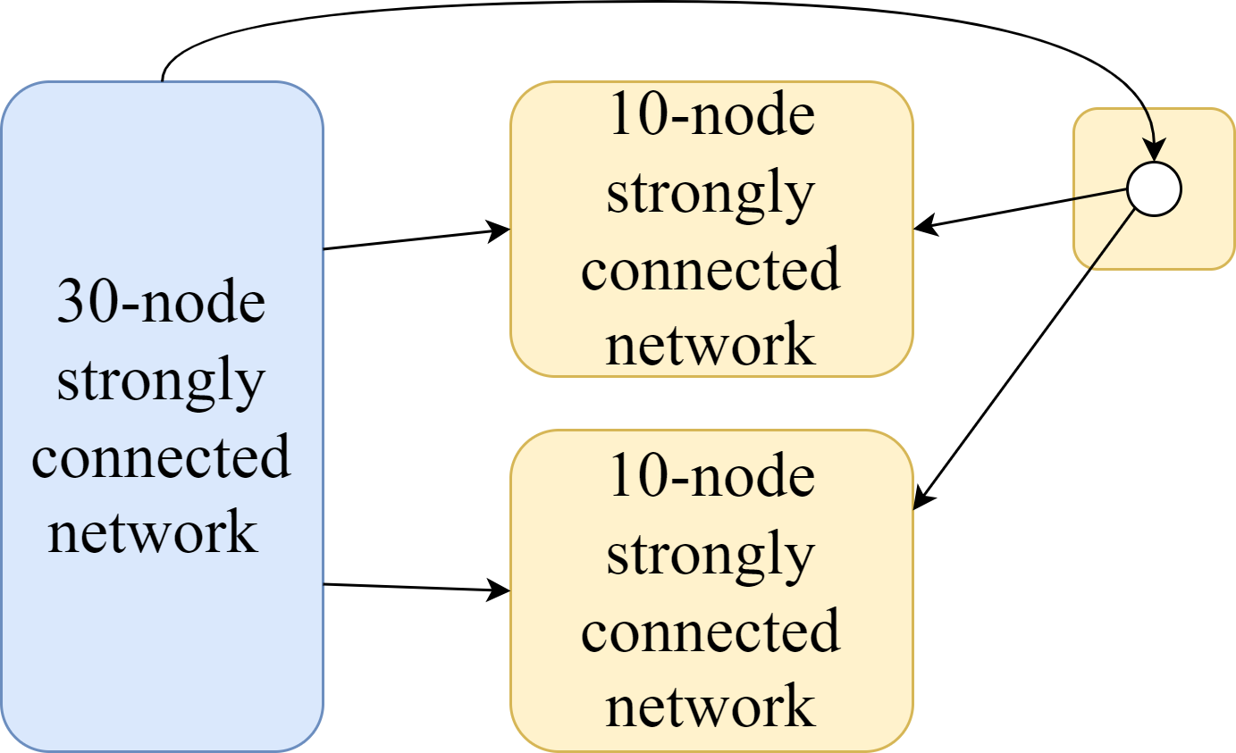
Figure 3: The 51-node communication network with spanning tree.

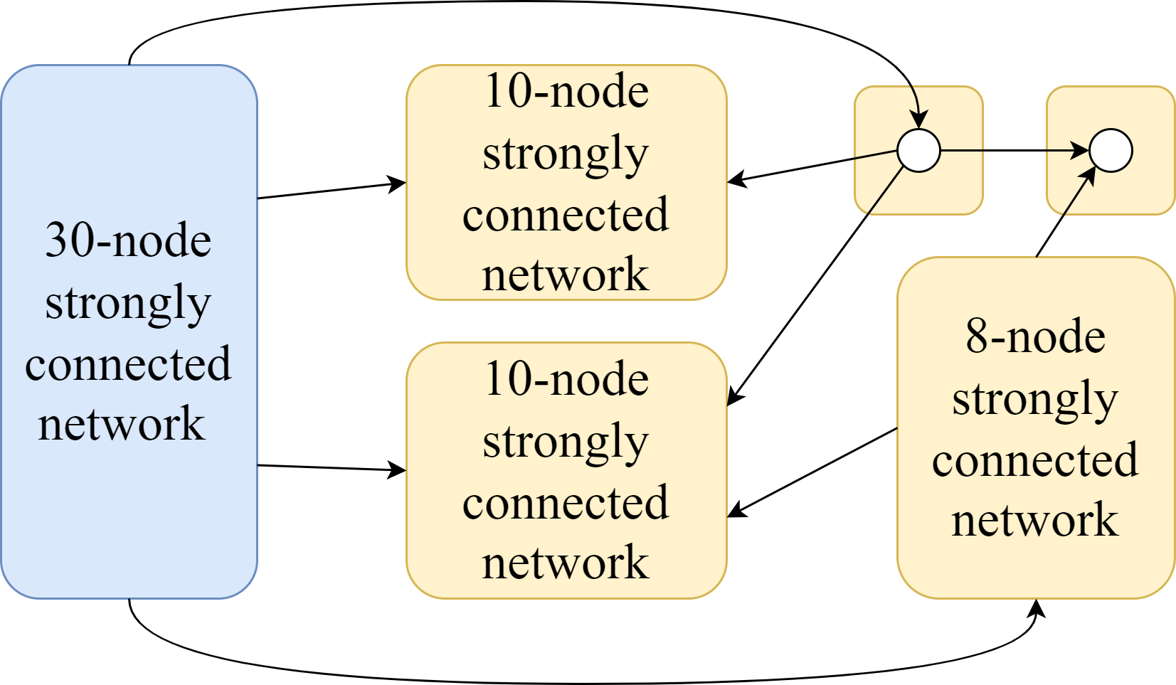
Figure 4: The 60-nodes communication network with spanning tree.

We provide three examples for both non-collaborative and collaborative protocol designs to verify our results.

5.1.1 Non-collaborative protocol design

Firstly, we choose the following continous-time MAS consisting of neutrally stable agents:

$$\left\{\;\begin{array}[]{l}\dot{x}_{i}={\begin{pmatrix}0&1\\ -1&0\end{pmatrix}}x_{i}+\begin{pmatrix}1\\ 1\end{pmatrix}u_{i}\\ y_{i}={\begin{pmatrix}1&0\end{pmatrix}}x_{i}\end{array}\right.$$ (21)

The agent model satisfies the conditions of Theorem 1. As such the agent, we can design a scale-free non-collaborative protocol based on the above agent model by using [7, Theorem 3].

$$\left\{\;\begin{array}[]{l}\dot{\eta}_{i}=-\eta_{i}-2\zeta_{i}\\ u_{i}=-\eta_{i}-2\zeta_{i}\end{array}\right.$$ (22)

Firstly, we consider scale-free state synchronization result for the 51-node and 60-node network shown in figures 3 and 4, which both contain a spanning tree. We obtain state synchronization as illustrated in figures 5 and 6 respectively. Since this specific protocol is scale free this is in line with the theoretical result that state synchronization is achieved when there exists a directed spanning tree for the network.

For discrete time MAS, we use the following agent model

$$\begin{array}[]{l}{x}_{i}(k+1)={\begin{pmatrix}0&1\\ -1&0\end{pmatrix}}x_{i}(k)+\begin{pmatrix}0\\ 1\end{pmatrix}u_{i}(k)\\ y_{i}(k)={\begin{pmatrix}1&0\end{pmatrix}}x_{i}(k)\end{array}$$ (23)

The agent model satisfies the conditions of Theorem 3 and we can design the following scale-free non-collaborative protocol by using [7, Theorem 5]:

$$\left\{\;\begin{array}[]{l}{\eta}_{i}(k+1)={\begin{pmatrix}0&1\\ -0.5&0\end{pmatrix}}\eta_{i}(k)+\begin{pmatrix}0\\ -0.5\end{pmatrix}\zeta_{i}(k)\\ u_{i}(k)={\begin{pmatrix}0.1&0\end{pmatrix}}\eta_{i}(k)\end{array}\right.$$ (24)

For the communication network in figure 4, we obtain synchronization as illustrated in figure 7.

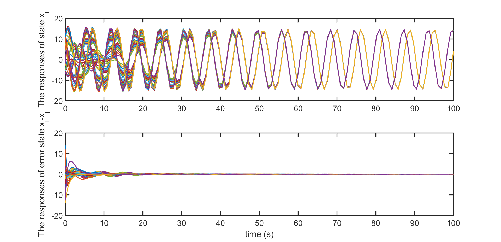
Figure 5: The state synchronization and error state results for 51-node continuous-time MAS via non-collaborative protocol.

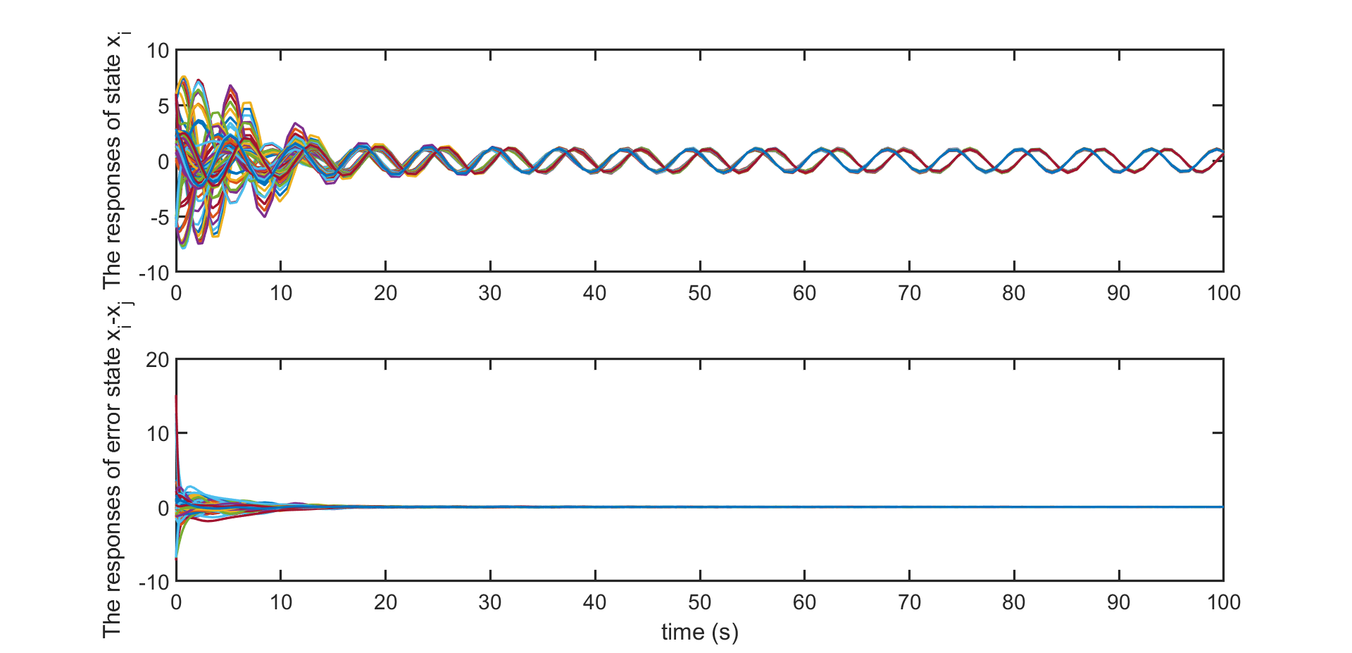
Figure 6: The state synchronization and error state results for 60-node continuous-time MAS via non-collaborative protocol.

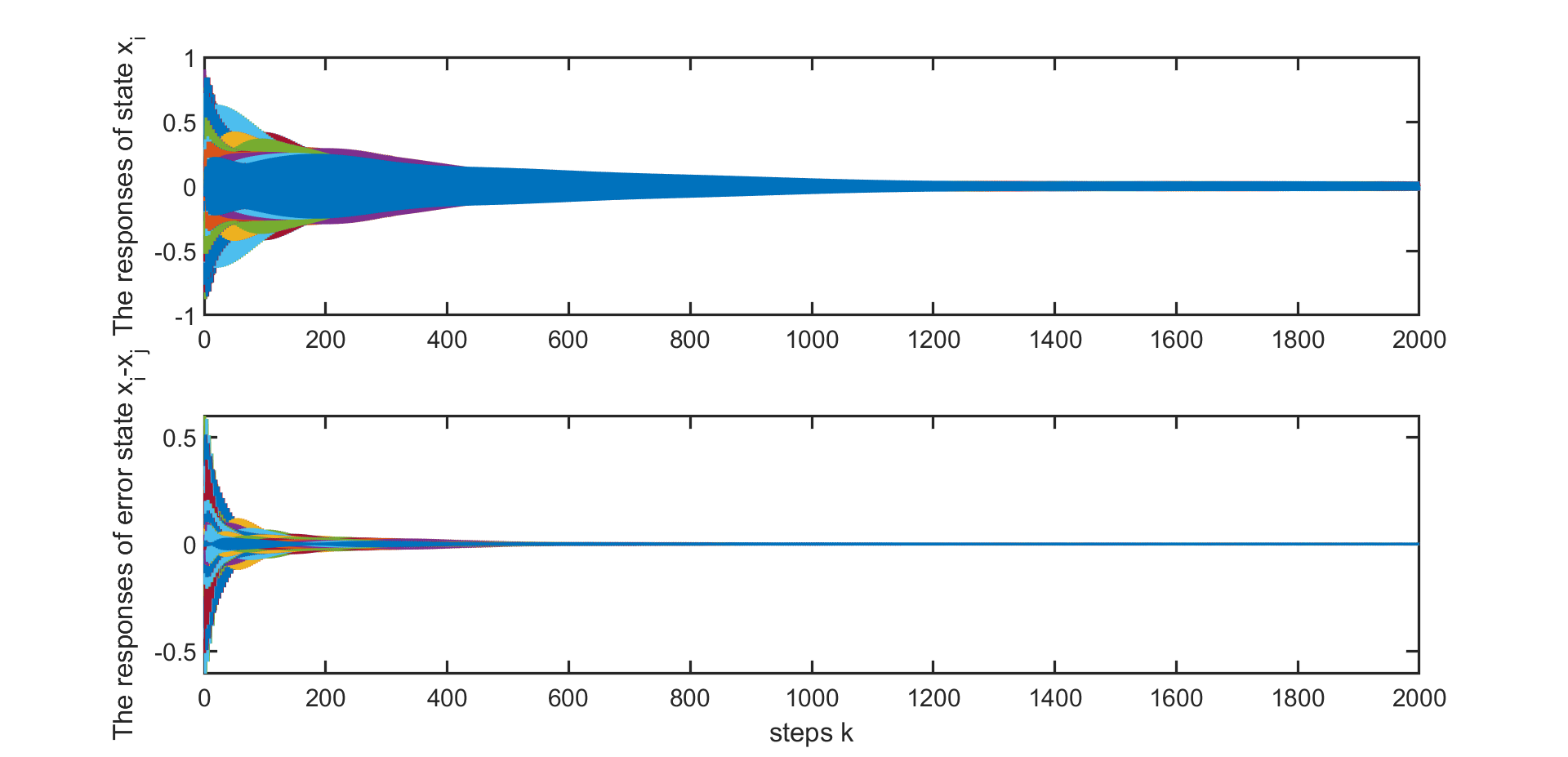
Figure 7: The state synchronization and error state results for discrete-time MAS via non-collaborative protocol.

5.1.2 Collaborative protocol design

Here, we consider a MAS consisting of double-integrator agents:

$$\begin{array}[]{l}\dot{x}_{i}={\begin{pmatrix}0&1\\ 0&0\end{pmatrix}}x_{i}+\begin{pmatrix}0\\ 1\end{pmatrix}u_{i}\\ y_{i}={\begin{pmatrix}1&0\end{pmatrix}}x_{i}\end{array}$$ (25)

The agent model satisfies the conditions of Theorem 5 and we design the scale-free collaborative protocol by using [6, Chapter 2].

$$\left\{\;\begin{array}[]{l}\dot{\hat{x}}_{i}={\begin{pmatrix}-1&1\\ -1&0\end{pmatrix}}\hat{x}_{i}+\begin{pmatrix}1\\ 1\end{pmatrix}\zeta_{i}-{\begin{pmatrix}0&0\\ 1&1\end{pmatrix}}\hat{\zeta}_{i}\\ \dot{\eta}_{i}={\begin{pmatrix}0&1\\ 0&0\end{pmatrix}}\eta_{i}+\begin{pmatrix}0\\ 1\end{pmatrix}u_{i}+\hat{x}_{i}-\hat{\zeta}_{i}\\ u_{i}=-{\begin{pmatrix}1&1\end{pmatrix}}\eta_{i}\end{array}\right.$$ (26)

where $\hat{\zeta}_{i}$ defined by (17) with $H_{c}=I$. We apply this scale-free protocol the two different networks given by 3 and 4. The theoretical results predict synchronization which is confirmed by our simulation as illustrated in Figures 8 and 9 respectively.

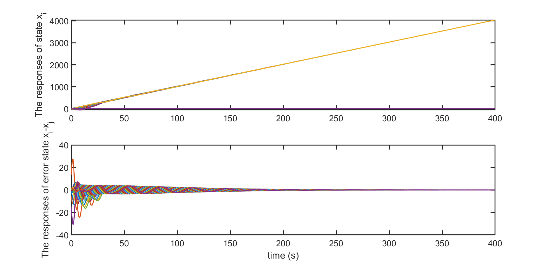
Figure 8: The state synchronization and error state results for 51-node continuous-time MAS via collaborative protocol.

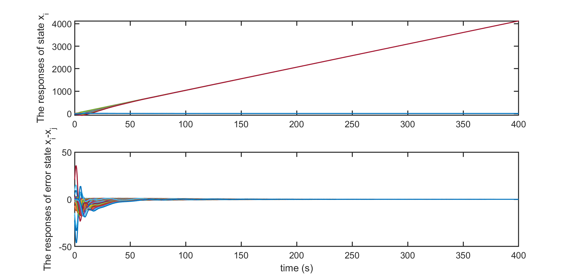
Figure 9: The state synchronization and error state results for 60-node continuous-time MAS via collaborative protocol.

5.2 Network without a directed spanning tree

When some links have faults in network so as to the links are broken, the communication network will loss its spanning tree. For example, two links are broken in the original 60-node network given by Fig. 3. We obtain the network as given in Figure 10

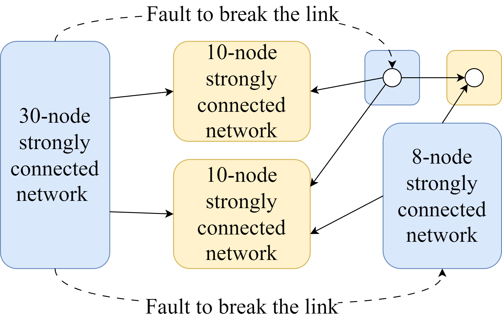
Figure 10: The communication network without spanning tree. Dashed lines denote that the links are broken due to faults.

It is obvious that there is no spanning tree in Figure 10. We obtain three basic bicomponents (indicated in blue): cluster 1 containing 30 nodes; cluster 2 containing 8 nodes and, finally, cluster 3 containing $1$ node. Moreover, we have three non-basic bicomponents: cluster 4 containing 10 nodes, cluster 5 containing 10 nodes, and cluster 6 containing 1 node, which are indicated in yellow.

5.2.1 Non-collaborative protocol

We consider again the continous-time MAS consisting of neutrally stable agent given by (21) with a scale-free protocol given by (22). For the original network given in figure 4 we obtained state synchronization since the network contained a directed spanning tree. But what happens for the network given by (10) which does not contain a directed spanning tree. In line with part 1 of Theorem 2, the three clusters 1, 2 and 3 which describe the three basic bicomponents of the network each achieve state synchronization within the cluster. However, the synchronized trajectories of these three clusters are not equal. See figures 11, 12 and 13. They all converge to sinusoids of the same frequency (prescribed by the agent dynamics) but with different phase and amplitude. Clusters 4, 5, and 6 represent non-basic bicomponents and the theory (part 2 of Theorem 2) states that they converge to a weighted average of the synchronized trajectories of clusters 1, 2 and 3. This is indeed the case as illustrated in figures 14, 15 and 16, respectively.

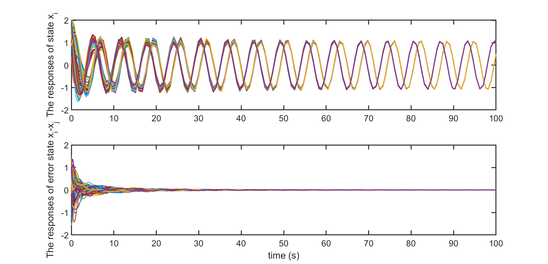
Figure 11: Cluster 1: The cluster state synchronization and error state result for 30-node basic bicomponent continuous-time MAS via non-collaborative protocol.

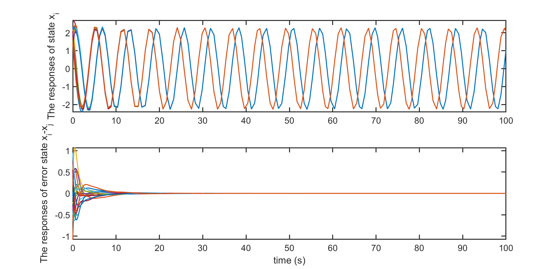
Figure 12: Cluster 2: The cluster state synchronization and error state result for 8-node basic bicomponent continuous-time MAS via non-collaborative protocol.

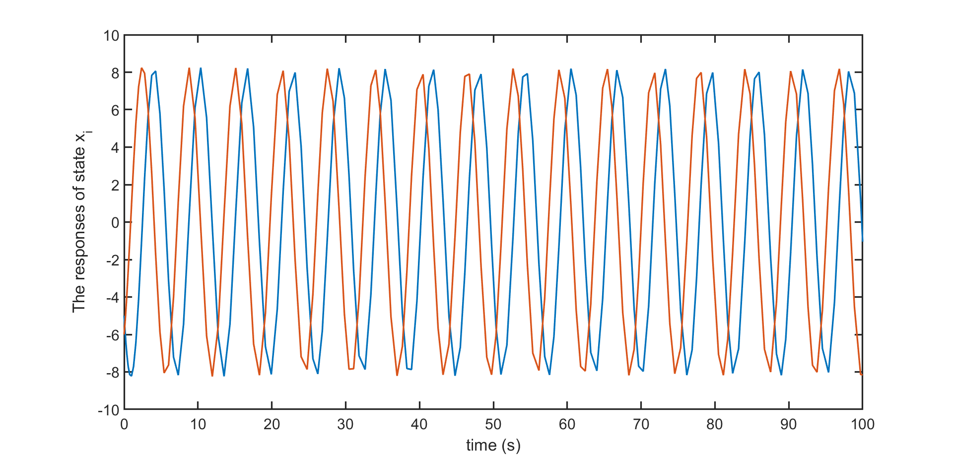
Figure 13: Cluster 3: The cluster state synchronization result for 1-node basic bicomponent continuous-time MAS via non-collaborative protocol. There is no error state cause it is only one agent.

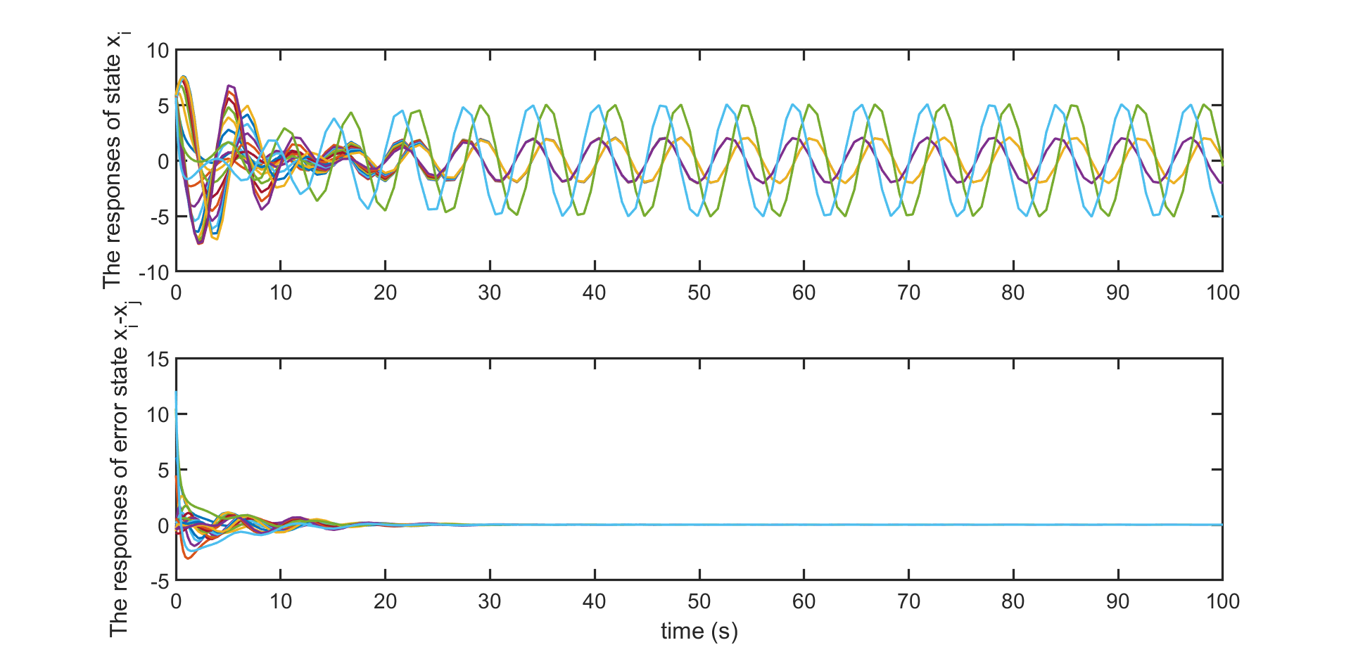
Figure 14: Cluster 4: The cluster state synchronization and error state result for 10-node non-basic bicomponent continuous-time MAS via non-collaborative protocol.

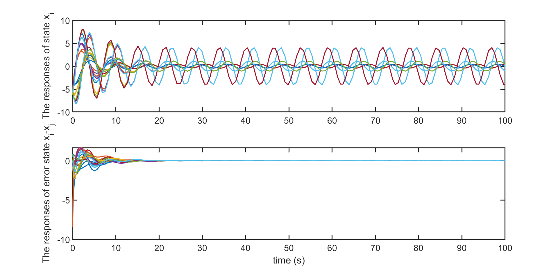
Figure 15: Cluster 5: The cluster state synchronization and error state result for 10-node non-basic bicomponent continuous-time MAS via non-collaborative protocol.

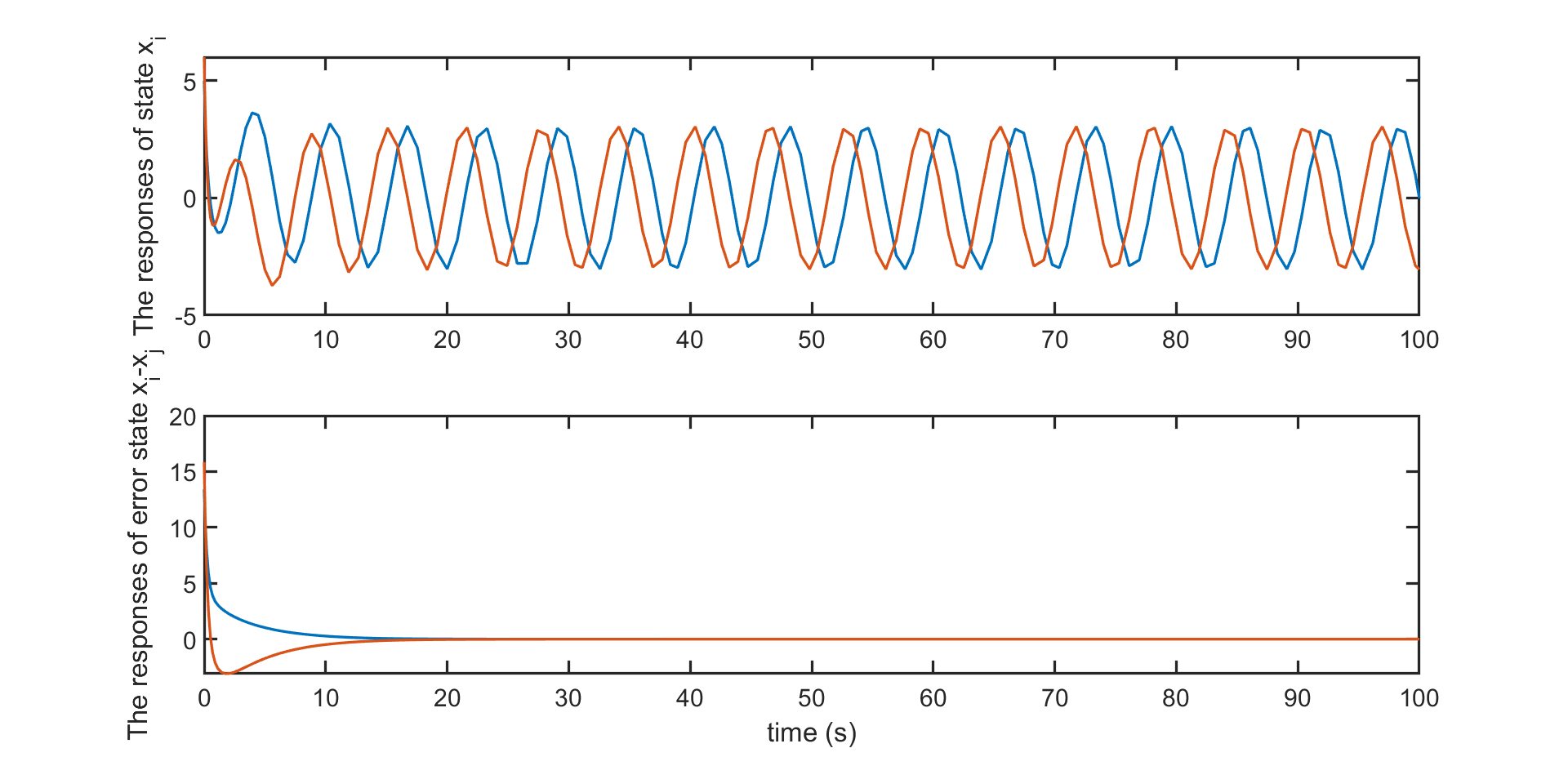
Figure 16: Cluster 6: The cluster state synchronization and error state result for 1-node non-basic bicomponent continuous-time MAS via non-collaborative protocol.

For the discrete-time MAS consisting of neutrally stable agent given by (23) with a scale-free protocol given by (24). For the original network given in figure 4 we obtained state synchronization since the network contained a directed spanning tree. We again want to illustrate what happens for the network given by (10) which does not contain a directed spanning tree. In line with part 1 of Theorem 4, the three clusters 1, 2 and 3 which describe the three basic bicomponents of the network each achieve state synchronization within the cluster. However, the synchronized trajectories of these three clusters are not equal. See figures 17, 18 and 19. They all converge to sinusoids of the same frequency (prescribed by the agent dynamics) but with different phase and amplitude. Clusters 4, 5, and 6 represent non-basic bicomponents and the theory (part 2 of Theorem 4) states that they converge to a weighted average of the synchronized trajectories of clusters 1,2 and 3. Like in continuous-time, this is indeed the case as illustrated in figures 20, 21, and 22, respectively.

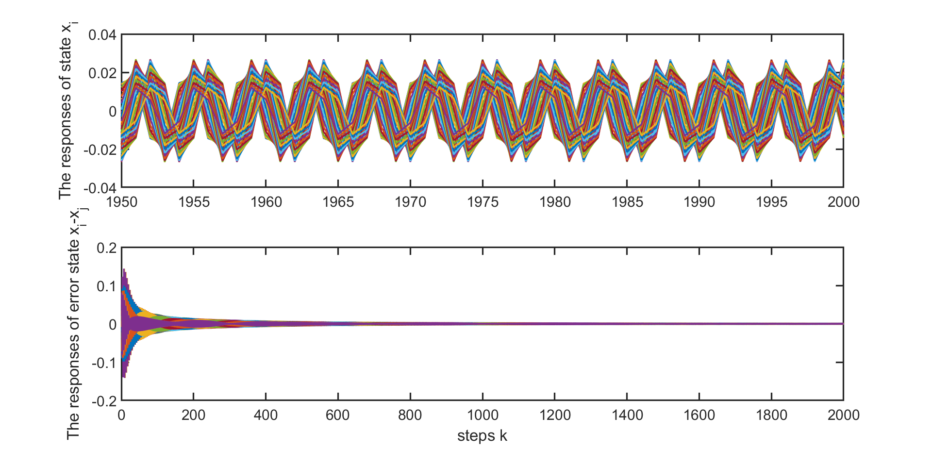
Figure 17: Cluster 1: The cluster state synchronization and error state result for 30-node basic bicomponent discrete-time MAS via non-collaborative protocol. Only the final trajectories are shown here to illustrate the result more clearly.

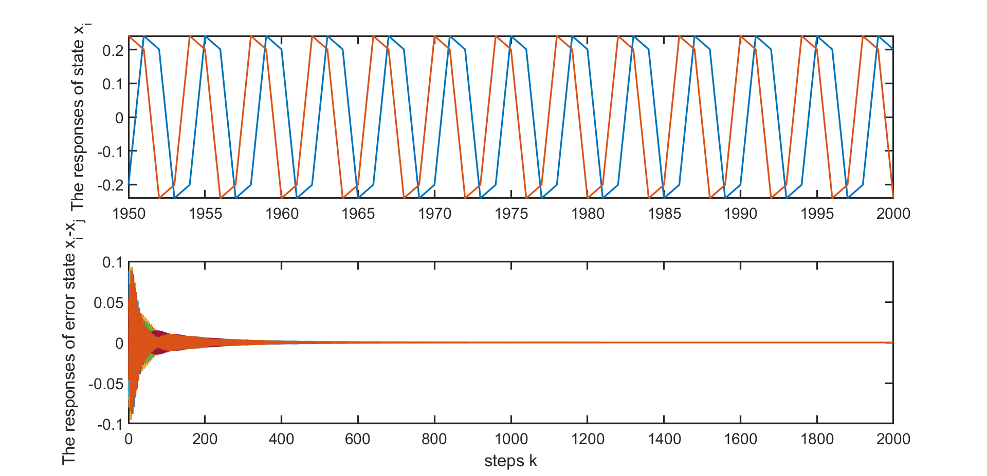
Figure 18: Cluster 2: The cluster state synchronization and error state result for 8-node basic bicomponent discrete-time MAS via non-collaborative protocol.

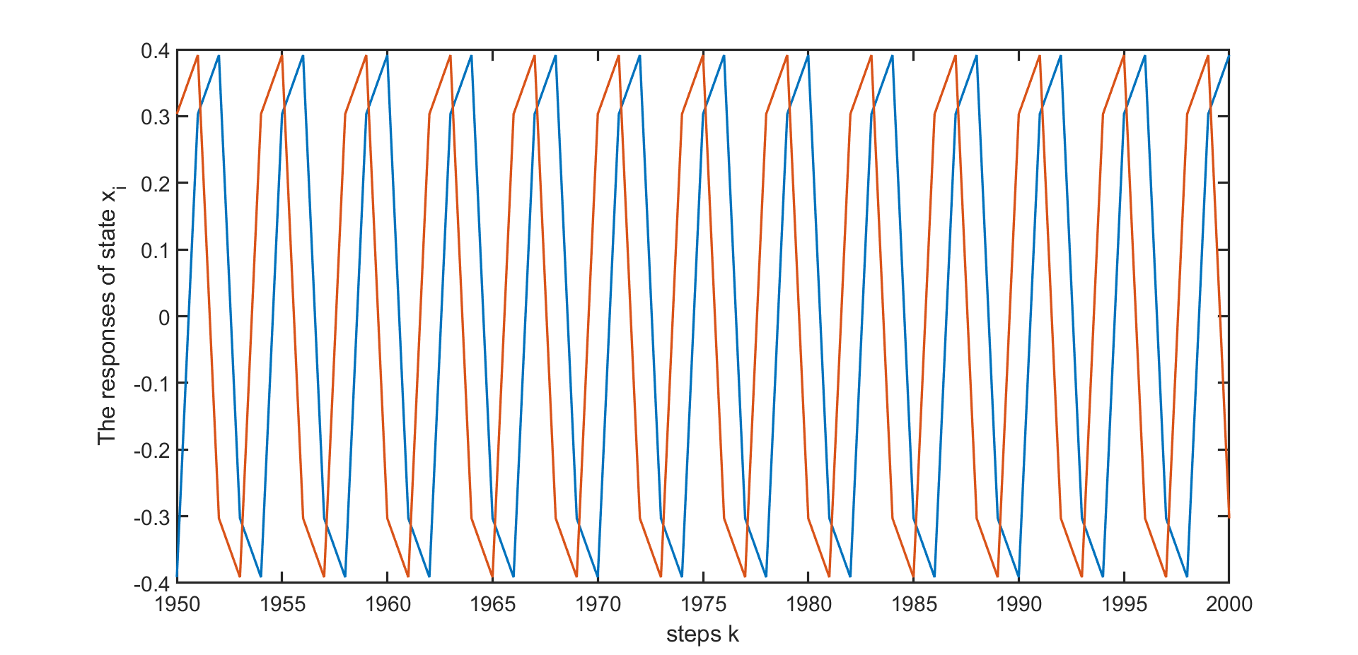
Figure 19: Cluster 3: The cluster state synchronization result for 1-node basic bicomponent discrete-time MAS via non-collaborative protocol.

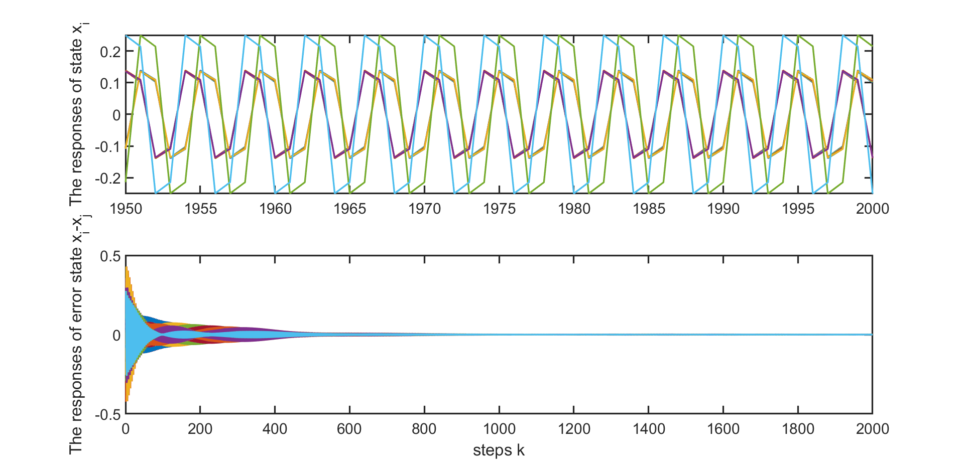
Figure 20: Cluster 4: The cluster state synchronization and error state result for 10-node non-basic bicomponent discrete-time MAS via non-collaborative protocol.

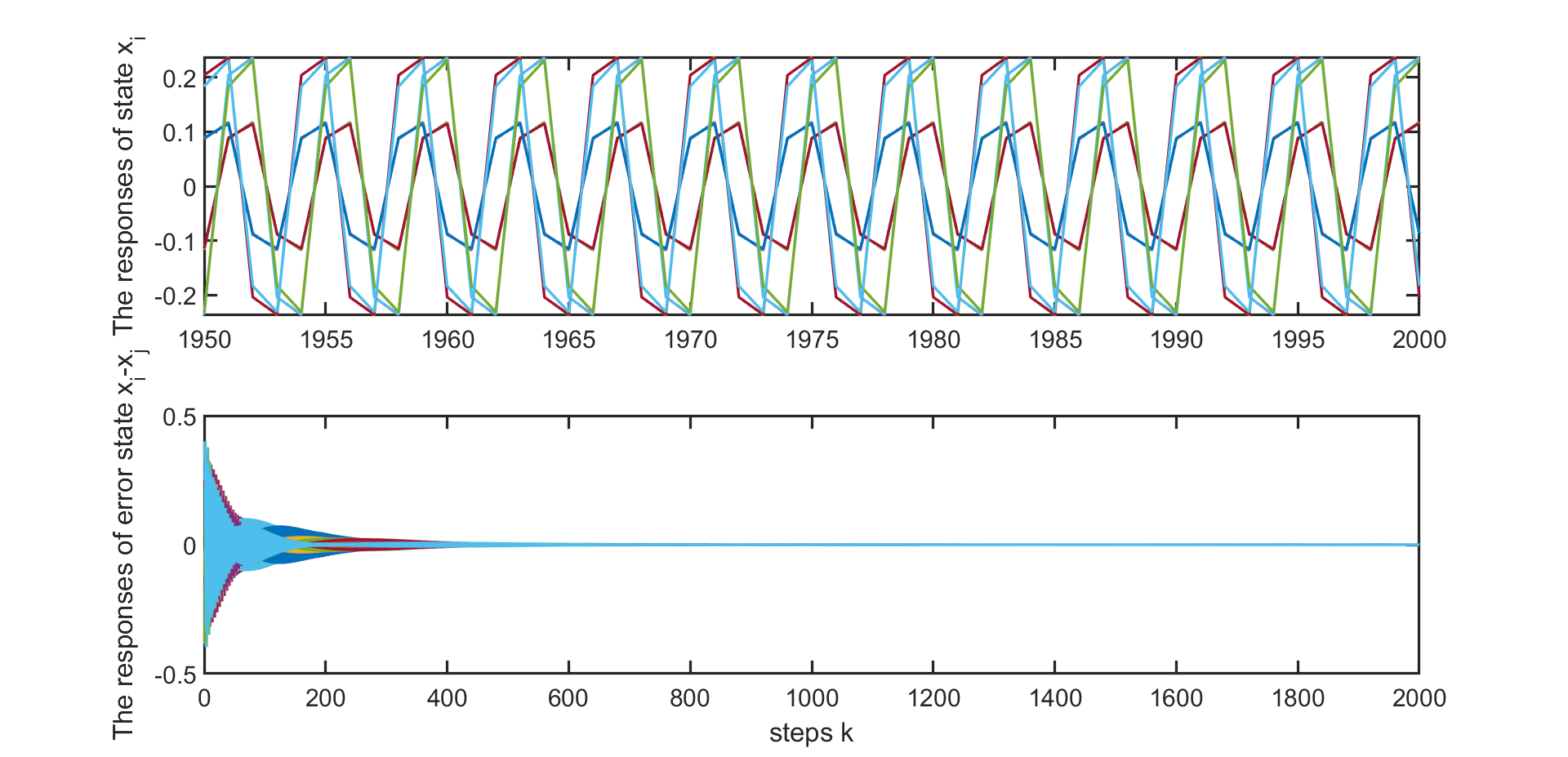
Figure 21: Cluster 5: The cluster state synchronization and error state result for 10-node non-basic bicomponent discrete-time MAS via non-collaborative protocol.

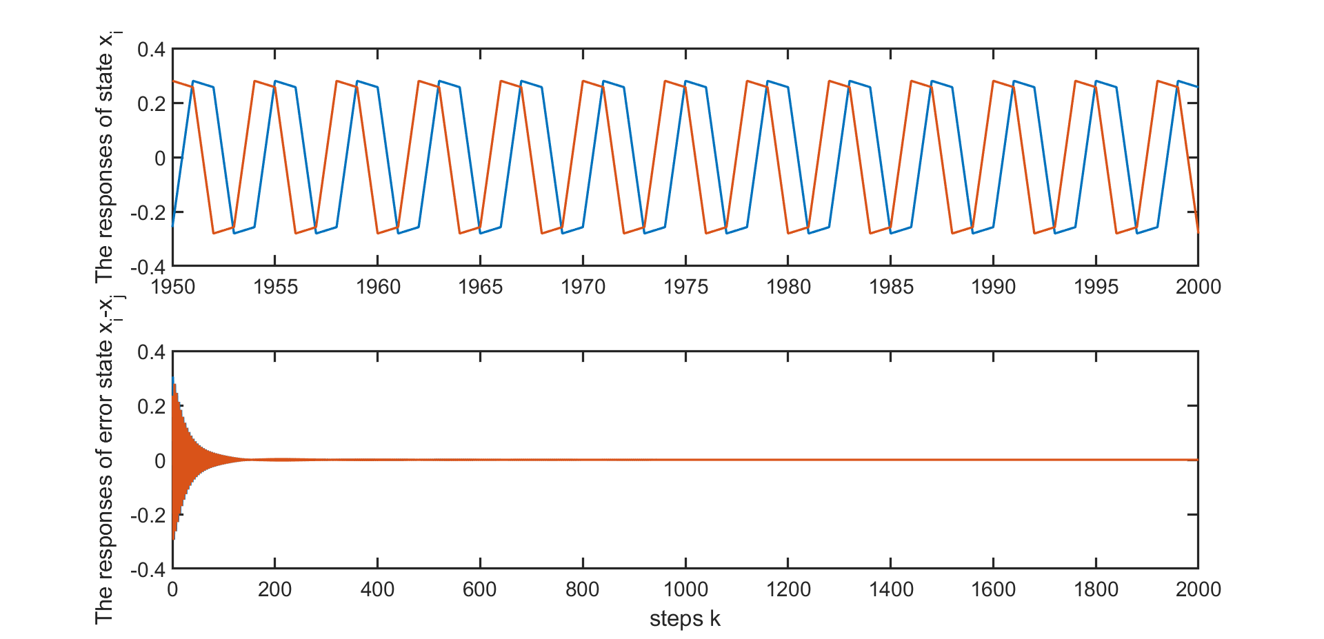
Figure 22: Cluster 6: The cluster state synchronization and error state result for 1-node non-basic bicomponent discrete-time MAS via non-collaborative protocol.

5.2.2 Collaborative protocol

Finally, for collaborative protocols, we consider a MAS consisting of double-integrator agent given by (25) and a scale-free collaborative protocol given by (26). We have seen that for the 60-node network given by (4) this protocol indeed achieves state synchronization. If we apply the same protocol to the network described by (10) which does not contain a directed spanning tree, we again consider the five bicomponents constituting the network. We see that, consistent with the theory, we get synchronization within clusters 1, 2 and 3 which are the three basic bicomponents as illustrated in figures 23, 24 and 25 respectively. The synchronized trajectory is this time no longer bounded due to the fact that the dynamics of the agents are double integrators and hence no longer bounded. The synchronized trajectory then becomes a line.

Clusters 4, 5, and 6 represent non-basic bicomponents and the theory (part 2 of Theorem 6) states that they converge to a weighted average of the synchronized trajectories of clusters 1, 2 and 3. Like in the non-collaborative case, this is indeed happening as illustrated in figures 26, 27, and 28, respectively.

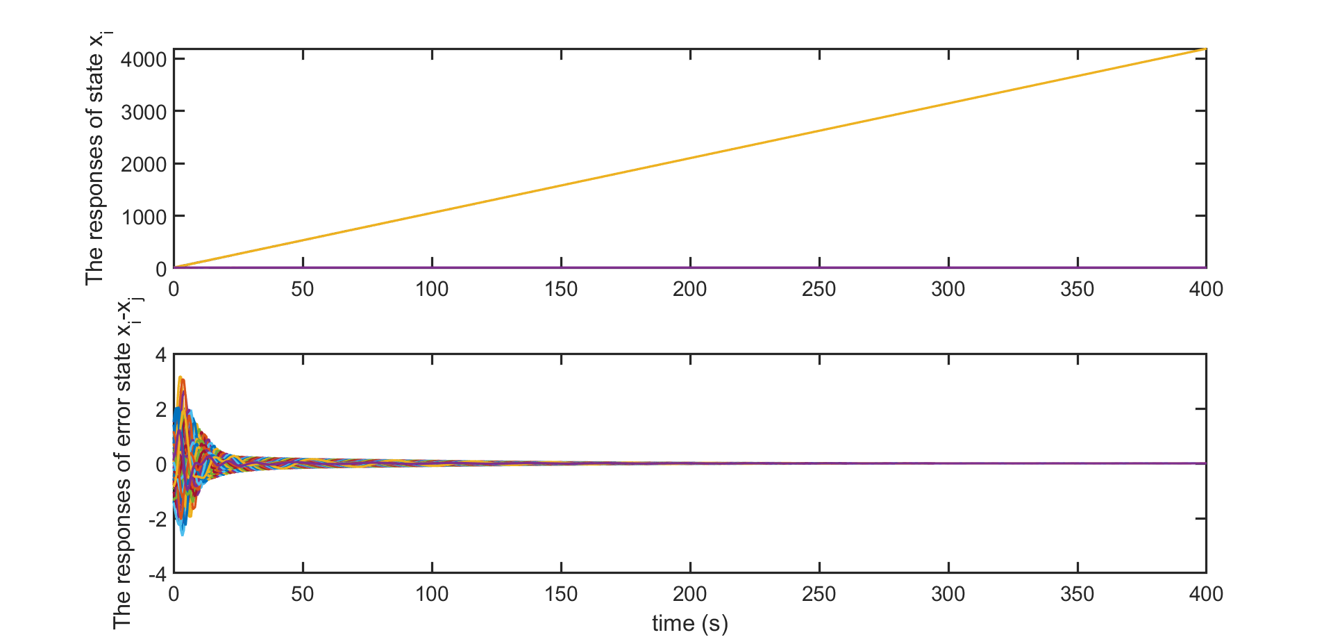
Figure 23: Cluster 1: The cluster state synchronization and error state result for 30-node basic bicomponent continuous-time MAS via collaborative protocol.

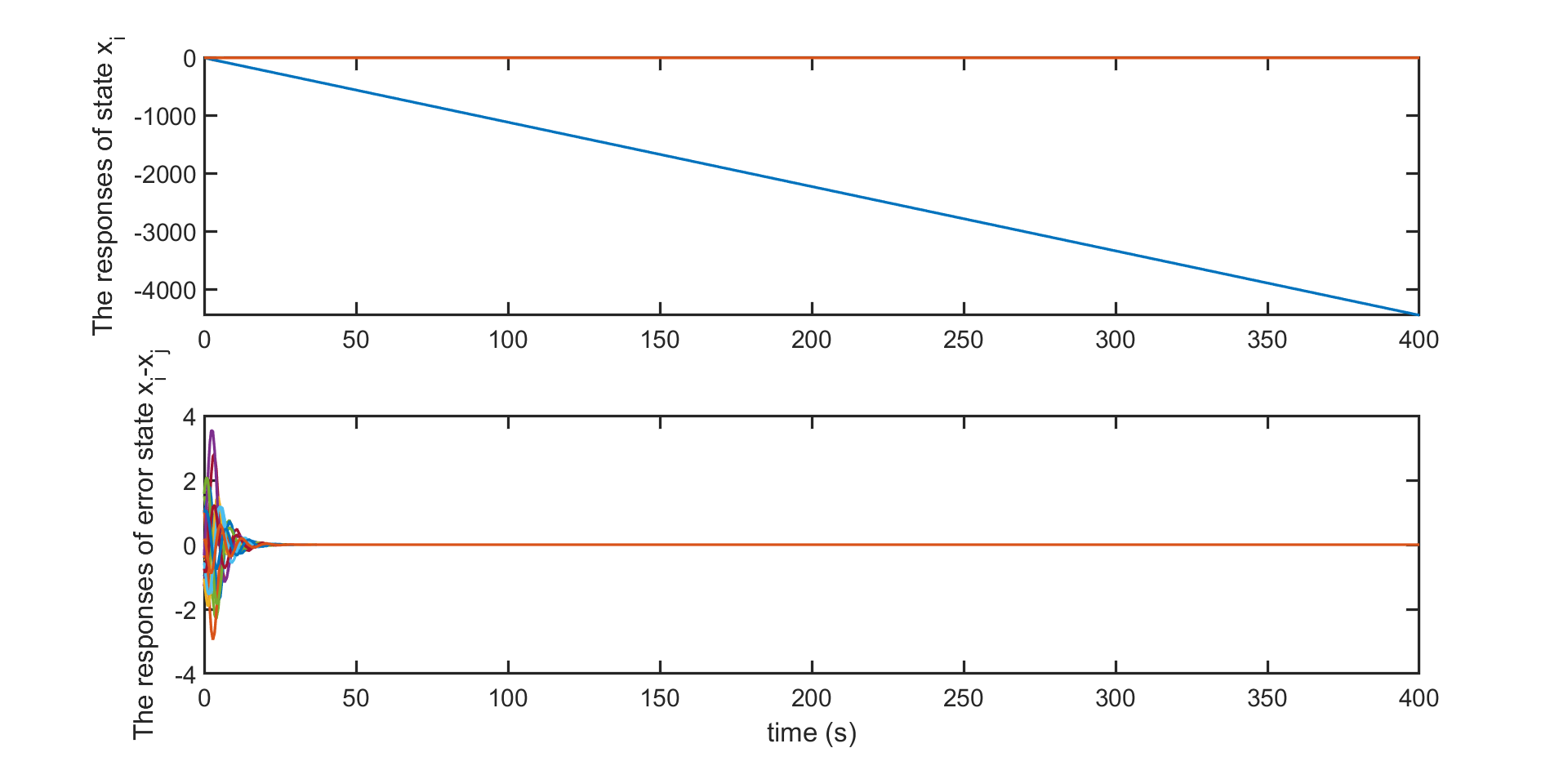
Figure 24: Cluster 2: The cluster state synchronization and error state result for 8-node basic bicomponent continuous-time MAS via collaborative protocol.

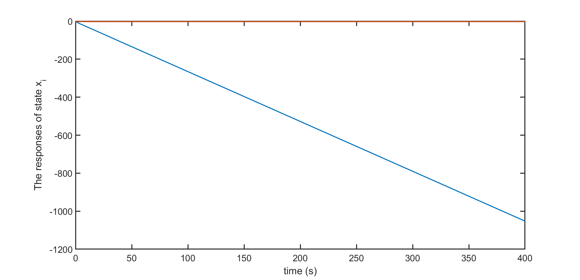
Figure 25: Cluster 3: The cluster state synchronization result for 1-node basic bicomponent continuous-time MAS via collaborative protocol.

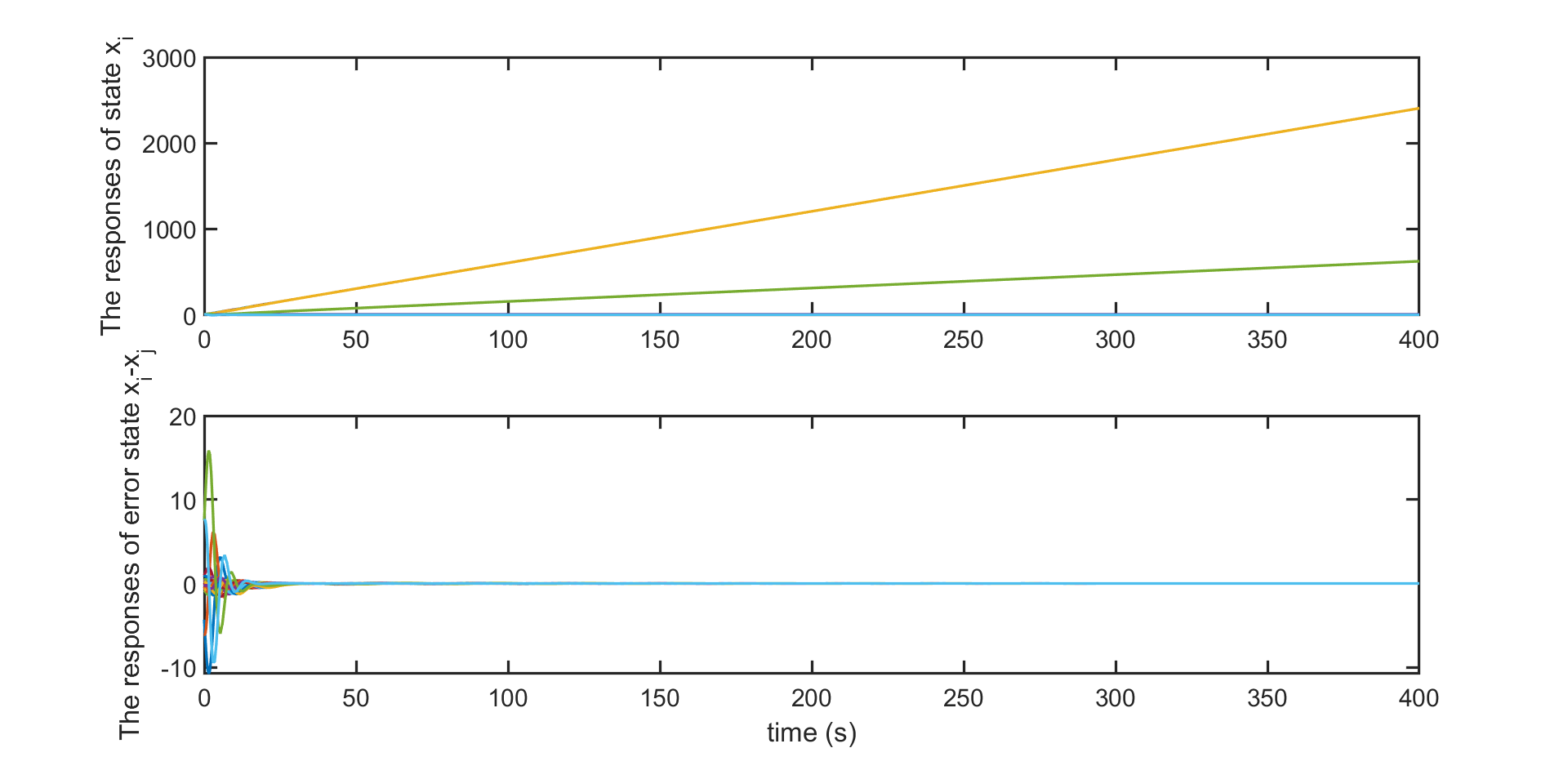
Figure 26: Cluster 4: The cluster state synchronization and error state result for 10-node non-basic bicomponent continuous-time MAS via collaborative protocol.

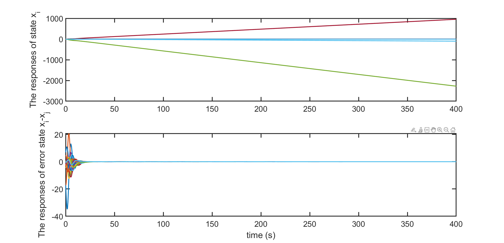
Figure 27: Cluster 5: The cluster state synchronization and error state result for 10-node non-basic bicomponent continuous-time MAS via collaborative protocol.

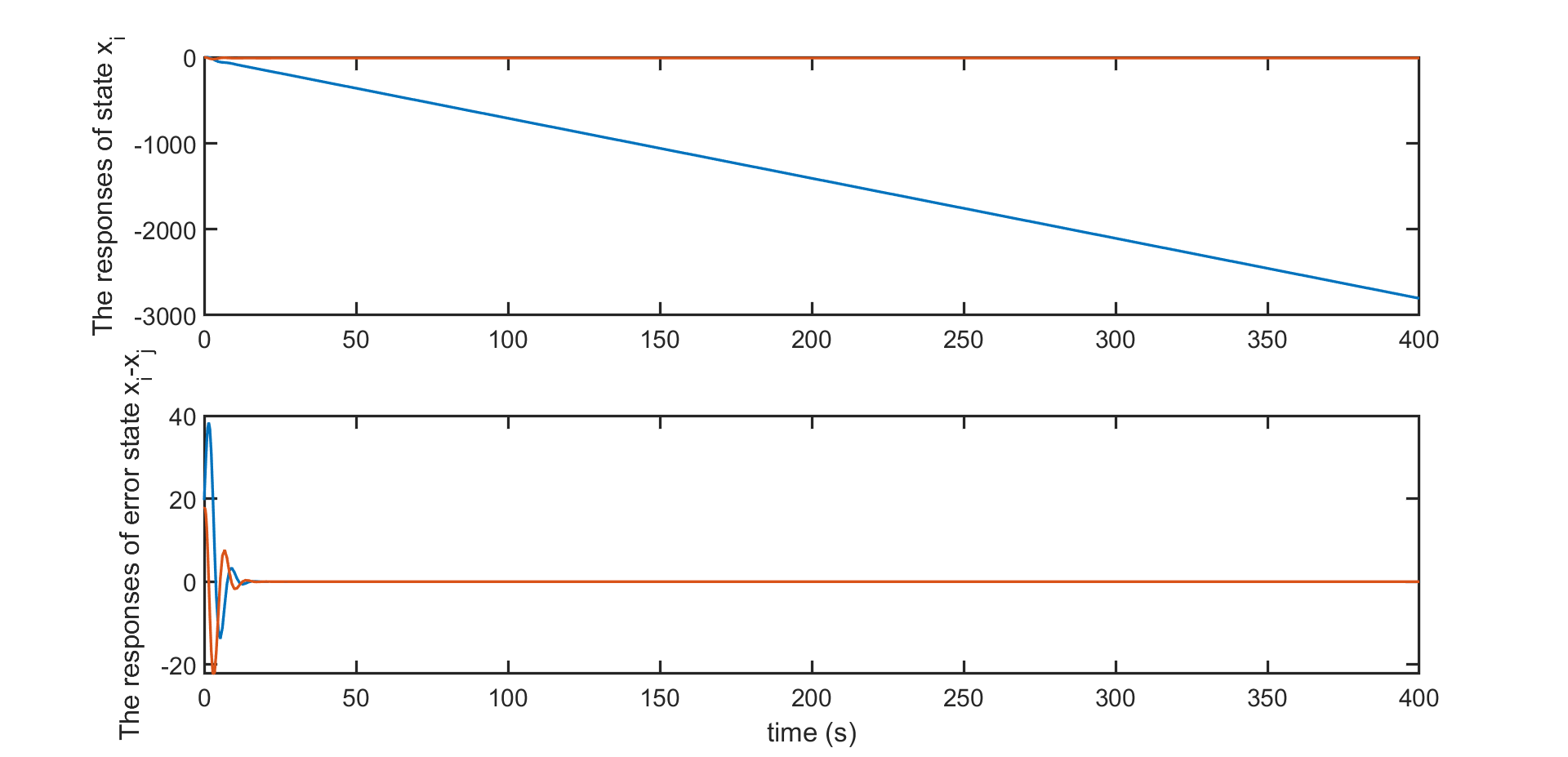
Figure 28: Cluster 6: The cluster state synchronization and error state result for 1-node non-basic bicomponent continuous-time MAS via collaborative protocol.

6 Conclusion

In this paper we have shown how scale-free protocols which achieve state synchronization behave when, due to a fault, the network no longer contains a directed spanning tree. We have seen that the protocols guarantee a stable response to these faults with achieving cluster synchronization which is clearly the best we could hope for in this scenario. This fault-tolerant behavior is a very attractive feature of scale-free protocols and makes them more feasible for practical applications.

References

- [1] H. Bai, M. Arcak, and J. Wen. Cooperative control design: a systematic, passivity-based approach. Communications and Control Engineering. Springer Verlag, 2011.
- [2] F. Bullo. Lectures on network systems. Kindle Direct Publishing, 2019.
- [3] C. Godsil and G. Royle. Algebraic graph theory, volume 207 of Graduate Texts in Mathematics. Springer-Verlag, New York, 2001.
- [4] L. Kocarev. Consensus and synchronization in complex networks. Springer, Berlin, 2013.
- [5] Z. Li, Z. Duan, G. Chen, and L. Huang. Consensus of multi-agent systems and synchronization of complex networks: A unified viewpoint. IEEE Trans. Circ. & Syst.-I Regular papers, 57(1):213–224, 2010.
- [6] Z. Liu, D. Nojavanzedah, and A. Saberi. Cooperative control of multi-agent systems: A scale-free protocol design. Springer, Cham, 2022.
- [7] Z. Liu, A. Saberi, and A.A. Stoorvogel. Scale-free non-collaborative linear protocol design for a class of homogeneous multi-agent systems. IEEE Trans. Aut. Contr., 2023. Published online, DOI:10.1109/TAC.2023.3324266.
- [8] M. Mesbahi and M. Egerstedt. Graph theoretic methods in multiagent networks. Princeton University Press, Princeton, 2010.
- [9] R. Olfati-Saber and R.M. Murray. Consensus problems in networks of agents with switching topology and time-delays. IEEE Trans. Aut. Contr., 49(9):1520–1533, 2004.
- [10] W. Ren and R.W. Beard. Consensus seeking in multiagent systems under dynamically changing interaction topologies. IEEE Trans. Aut. Contr., 50(5):655–661, 2005.
- [11] W. Ren and Y.C. Cao. Distributed coordination of multi-agent networks. Communications and Control Engineering. Springer-Verlag, London, 2011.
- [12] A. Saberi, A. A. Stoorvogel, M. Zhang, and P. Sannuti. Synchronization of multi-agent systems in the presence of disturbances and delays. Birkhäuser, New York, 2022.
- [13] A. Stanoev and D. Smilkov. Consensus theory in networked systems. In L. Kocarev, editor, Consensus and synchronization in complex networks, pages 1–22. Spinger-Verlag, Berlin, 2013.
- [14] S. Stüdli, M. M. Seron, and R. H. Middleton. Vehicular platoons in cyclic interconnections with constant inter-vehicle spacing. In 20th IFAC World Congress, volume 50(1) of IFAC PapersOnLine, pages 2511–2516, Toulouse, France, 2017. Elsevier.
- [15] E. Tegling, B. Bamieh, and H. Sandberg. Localized high-order consensus destabilizes large-scale networks. In American Control Conference, pages 760–765, Philadelphia, PA, 2019.
- [16] E. Tegling, B. Bamieh, and H. Sandberg. Scale fragilities in localized consensus dynamics. Automatica, 153(111046):1–12, 2023.
- [17] E. Tegling, R. H. Middleton, and M. M. Seron. Scalability and fragility in bounded-degree consensus networks. In 8th IFAC Workshop on Distributed Estimation and Control in Networked Systems, volume 52(20), pages 85–90, Chicago, IL, 2019. IFAC-PapersOnLine, Elsevier.
- [18] C.W. Wu. Synchronization in complex networks of nonlinear dynamical systems. World Scientific Publishing Company, Singapore, 2007.