Mistake, Manipulation and Margin Guarantees in Online Strategic Classification
Abstract
We consider an online strategic classification problem where each arriving agent can manipulate their true feature vector to obtain a positive predicted label, while incurring a cost that depends on the amount of manipulation. The learner seeks to predict the agent’s true label given access to only the manipulated features. After the learner releases their prediction, the agent’s true label is revealed. Previous algorithms such as the strategic perceptron guarantee finitely many mistakes under a margin assumption on agents’ true feature vectors. However, these are not guaranteed to encourage agents to be truthful. Promoting truthfulness is intimately linked to obtaining adequate margin on the predictions, thus we provide two new algorithms aimed at recovering the maximum margin classifier in the presence of strategic agent behavior. We prove convergence, finite mistake and finite manipulation guarantees for a variety of agent cost structures. We also provide generalized versions of the strategic perceptron with mistake guarantees for different costs. Our numerical study on real and synthetic data demonstrates that the new algorithms outperform previous ones in terms of margin, number of manipulation and number of mistakes.
1 Introduction
Binary classification is a well-known problem in supervised learning, with applications in numerous important domains such as marketing, finance, natural language processing and medicine. The traditional binary classification problem aims to learn a decision rule that maps feature vectors to binary labels , with the aim of predicting a true underlying label for a feature vector. For example, features may correspond to identifying information of customers of a bank who apply for a loan, and in this context the label may indicate whether the bank will approve or deny the loan. The true underlying label, whether the bank should approve or deny given all future outcomes, is unknown at the time of the loan application, which necessitates the need to use a classification rule.
Like the example above, binary classification is now regularly applied to various applications involving human agents. Customers obviously prefer that their loan application be approved rather than denied, and in many other applications there may similarly be one label that is preferred by agents over the other. One can imagine that in practice this leads to strategic behavior of agents, where feature vectors are manipulated in order to achieve the desired label prediction. Of course, there is often also a cost associated with manipulation, so agents may manipulate only if the payoff for achieving the desirable label is worth the cost.
Amidst potential misleading strategic behavior of agents, the learner wishes to find a decision rule that still accurately predicts the true underlying label, despite given access to only potentially manipulated feature vectors. This is the problem of strategic classification. In this paper, we study an online model for strategic classification with continuous features (i.e., feature vectors are in ), where agents arrive sequentially, observe the current decision rule, and present their potentially manipulated feature vectors to the learner. Upon each arrival, the learner uses the current decision rule to classify, i.e., predict the label of the agent. Then, the true label is revealed, and the learner may update the decision rule based on the revealed information of the agent’s potentially manipulated feature vector and true label.
1.1 Literature
The idea of strategic agents dates back to Brückner and Scheffer [2011], Dalvi et al. [2004], Dekel et al. [2008], where the focus is on agents’ adversarial behavior. In this setting, the agents’ goal is to completely mislead the learner, and the agents are agnostic to the label they receive. The strategic classification problem as described above, where agents have preferences over labels and behave in a self-interested fashion, is introduced by Hardt et al. [2016], where a Stackelberg game is used to model the learner (leader) and agent (follower) behavior.
Strategic classification is studied in two settings: (i) the offline setting in which data points come from an underlying distribution and the learner aims to find the equilibrium of the resulting Stackelberg game; and (ii) in the online setting where the data points arrive sequentially and the learner has the opportunity to revise their classifier. In the offline setting the focus has been on developing methods to approximately compute the Stackelberg equilibrium, and understanding their sample complexity [Hardt et al., 2016, Zhang and Conitzer, 2021, Sundaram et al., 2023, Lechner and Urner, 2022, Perdomo et al., 2020, Zrnic et al., 2021]. On the other hand, the algorithms in the online setting aim to minimize the Stackelberg regret [Chen et al., 2020, Dong et al., 2018, Ahmadi et al., 2023] or the number of mistakes over a time horizon [Ahmadi et al., 2021, 2023]. As mentioned above, our work studies the latter online setting, and we analyze the number of mistakes, manipulations and convergence of the classifiers over time.
The strategic classification literature can also be categorized based on the assumptions on the agent manipulation structures. The most common assumption is continuous manipulation of feature vectors in , where any perturbation of the feature vectors is possible within a bounded set and the cost is a continuous function (typically a weighted norm) [Dong et al., 2018, Chen et al., 2020, Haghtalab et al., 2020, Ahmadi et al., 2021, Ghalme et al., 2021, Sundaram et al., 2023]. Alternatively, a discrete manipulation structure where only some manipulations are plausible, defined through a manipulation graph, is also studied in [Lechner and Urner, 2022, Zhang and Conitzer, 2021, Ahmadi et al., 2023]. Relatedly, some works have focused on relaxing assumptions on the learner-agent interaction model, such as allowing for imperfect information [Ghalme et al., 2021, Bechavod et al., 2022, Jagadeesan et al., 2021] and collective agent actions [Zrnic et al., 2021]. Ghalme et al. [2021], Bechavod et al. [2022], Jagadeesan et al. [2021] all examine the offline problem, while Zrnic et al. [2021] considers the online problem where the agents’ learn their best actions collectively and over time. In contrast, our work examines the online model, with continuous manipulations, and we consider the standard full information learner-agent interaction model, where agents are individualistic and can respond optimally instantly.
Another concept worth mentioning, although not yet formalized in the literature, is the ability of an algorithm to encourage truthfulness of agents, by presenting classifiers which do not incentivize agents to manipulate their features. In contrast to earlier work [Hardt et al., 2016] that mainly focused on the misclassification error of an algorithm as a performance metric, Zhang and Conitzer [2021], Lechner and Urner [2022] take the vulnerability to manipulation into account. In particular, Zhang and Conitzer [2021] propose an algorithm that prevents strategic behaviors, and Lechner and Urner [2022] propose a strategic empirical manipulation loss that balances the classification accuracy and manipulation. Nevertheless, the context therein is different to ours: these works all consider the model of manipulation graph and offline learning, and their results mainly involve sample complexity analysis.
The possibility of strategic manipulation of feature vectors has also brought up a number of other closely related questions. In particular, Kleinberg and Raghavan [2020], Miller et al. [2020], Ahmadi et al. [2022], Bechavod et al. [2022], Shavit et al. [2020], Haghtalab et al. [2020], Alon et al. [2020], Tsirtsis et al. [2024] study how the agents can be incentivized to actually improve their qualification and eventually changing their true labels. [Hu et al., 2019, Milli et al., 2019, Braverman and Garg, 2020, Levanon and Rosenfeld, 2021] examine the societal implications of strategic behaviors. Strategic behaviors in other machine learning tasks such as linear regression have also gained interest [Chen et al., 2018, Bechavod et al., 2021].
Our setting is closest to Dong et al. [2018], Chen et al. [2020], Ahmadi et al. [2021], which all consider the online strategic classification problem with continuous feature manipulation model. In particular, Dong et al. [2018] study the online strategic classification problem with interaction between the agent and the learner, where the agent sends to the learner the best response that maximizes the agent’s utility function, and the learner suffers from a certain loss for misclassification. In order to derive a regret-minimizing algorithm, they identify conditions on the structure of agent’s utility function under which the learner’s problem is convex. Subsequently, whenever their proposed conditions are met, they propose an algorithm achieving a sublinear regret when the learner receives a mixture of strategic and non-strategic data points in an online manner. Our algorithms, in contrast, focus on different performance measures such as mistake bounds and margin guarantees. Moreover, we assume all data points are subject to manipulation whenever they have sufficient budget, whereas their algorithm essentially relies on the fraction of non-strategic data points. Chen et al. [2020] make a more general assumption on the agent’s utility function and deal with the case where the exact form of the utility function is unknown to the learner. In this setting, they propose an algorithm that relies on a special oracle, and provide a Stackelberg regret guarantee for their algorithm. Although their algorithm does not rely on the specific structure of the agent’s utility, their oracle access based model and analysis rely on fundamentally different assumptions than ours. Ahmadi et al. [2021] consider two specific families of manipulation cost functions based on - and weighted -norms. They generalize the well-known perceptron algorithm to the strategic setting and establish finite mistake bounds. In our paper, we generalize their algorithms and results to more general norms, suggest two new algorithms with theoretical guarantees on the number of mistakes, the number of manipulations and convergence to the best margin classifier for the classification problem based on the agents’ true features and show that our algorithms have superior practical performance as well.
Our new algorithms are generalizations of maximum margin classifiers to the strategic setting. For non-strategic classification, online algorithms for finding maximum margin classifiers have been studied in number of works [Li and Long, 1999, Gentile, 2002, Freund and Schapire, 1999, Frieß et al., 1998, Kivinen et al., 2004, Kowalczyk, 2000]. These propose scalable algorithms that update incrementally like the perceptron, aimed at finding a classifier with margin guarantees analogous to the support vector machine. We develop tools to address intricacies of the strategic setting and establish that max-margin algorithms in similar spirit can be developed in strategic setting as well even though none of our algorithms are generalization of these works.
1.2 Outline and contributions
Section 2 gives the formal problem setting of online strategic classification, introducing our notation and defining critical concepts such as cost of manipulation, agent response, margins and proxy data. In Section 3, we describe three algorithms for solving the online strategic classification problem with linear classifiers. The first two of our algorithms are aimed at recovering the maximum margin classifier in the presence of strategic behavior, while the third is a generalization of the strategic perceptron from [Ahmadi et al., 2021]. Our theoretical contributions can be summarized as follows:
-
•
We study the concept of proxy data which is constructed from agent responses after their true label has been revealed, and show that it plays a critical role in the design of algorithms in the presence of strategic behavior. In Section 3 we provide a condition (see Corollary 1) that ensures the proxy data to remain separable, which is critical for Algorithms 1, 2 and 3. It is noteworthy to mention that even if the classification problem based on the true feature vectors may be separable, as the agent responses and consequently their proxies built are functions of the classifiers released to the agents, ensuring the separability of the proxy data is in no way obvious or guaranteed. This is thus one of the key challenges in the strategic setting, and our solution to this issue forms the crux for developing sensible classification algorithms in the strategic setting.
-
•
Algorithm 1, described in Section 3.1, solves an offline maximum margin problem at each iteration on the proxy data. Through tools from convex analysis (given in Section 4.1), in Section 4.2 we provide explicit finite bounds on the number of mistakes and manipulations Algorithm 1 can make (Theorems 1 and 2). Furthermore, under a probabilistic data generation assumption, we show that Algorithm 1 almost surely recovers the maximum margin classifier for the non-manipulated agent features (Theorem 3) even through it has access to only (possibly) manipulated features of the agents.
-
•
In each iteration, Algorithm 1 solves an optimization problem of growing size. To mitigate the possibly expensive per-iteration cost of Algorithm 1, in Section 3.2 we describe Algorithm 2, which is an approximate version of Algorithm 1, inspired by the Joint Estimation and Optimization (JEO) framework [Ahmadi and Shanbhag, 2014, Ho-Nguyen and Kılınç-Karzan, 2021]. Algorithm 2 replaces the need to solve a full maximum margin problem at each iteration with a subgradient-type update. In Section 4.3, we use tools from online convex optimization to give conditions under which Algorithm 2 enjoys finite mistake and manipulation guarantees, and under the same probabilistic data generation assumption used for Algorithm 1, we show that Algorithm 2 also almost surely recovers the maximum margin classifier on non-manipulated agent features (Theorem 4).
-
•
Algorithm 3, described in Section 3.3, is a generalized version of the strategic perceptron developed by Ahmadi et al. [2021], who also provided mistake bounds for the strategic setting when the agent manipulation costs are based on - or weighted -norm. (In particular, Ahmadi et al. [2021] generalizes bounds for the classical non-strategic setting [Rosenblatt, 1958, Novikoff, 1962].) In Section 4.4, we use online convex optimization tools to provide mistake bounds for more general cost functions (Theorems 5 and 6). Moreover, our methods give improved mistake bounds in cases where the optimal linear classifier may not pass through the origin, without requiring information on the maximum margin (Remark 2). Our generalized version can also exploit a priori domain information of the classifier (whenever present) via a projection step to provide improved bounds in certain settings (Theorem 7).
-
•
In Section 4.5 we examine the assumptions that are used in developing our performance guarantees. Through various examples, we show that removing any of these will result in failure of the bounds, thus demonstrating the necessity of these assumptions. In particular, we show that the strategic perceptron algorithm of Ahmadi et al. [2021] as well as its generalization given in Algorithm 3 may incur infinitely many manipulations, and consequently may fail to converge to the max-margin classifier.
In Section 5 we test the numerical performance of our algorithms in terms of the number of mistakes, number of manipulations, and distance to the non-strategic maximum margin classifier. using real data from a lending platform as well as synthetic data. We show that Algorithm 1 generally has superior performance on all three metrics, and Algorithm 2 often outperforms Algorithm 3.
1.3 Notation
Let for any positive integer . Let denote the nonnegative orthant of the -dimensional Euclidean space. We define be the set of minimizers and the set of maximizers of the problems respectively. For a given convex (resp. concave) function , let be the subdifferential (resp. superdifferential) set of at . For a given function differentiable at , let denote the gradient of evaluated at . Let denote the convex hull of the set . Let be the -norm, i.e., for any . We define to be the unit -norm ball.
2 Problem Setting
In this section we formalize the problem definition for strategic classification. Each agent comprises of a data pair , where is a feature vector and is the associated label. Here, is a function mapping feature vectors in to , and is the space of all possible feature vectors. For notational convenience, we also define the sets of positively and negatively labeled agents, respectively, as
| (1) |
We focus on the case of continuous feature vectors and consider the set of linear classifiers parametrized by : given a feature vector , the predicted label for is defined to be
where we follow the convention of .
2.1 Manipulation and agent responses
In the strategic setting, labels of are assumed to be more desirable than . Therefore, an agent may manipulate their own true feature vector to change their predicted label, as long as it does not cost them too much. More precisely, we define the cost of manipulating a feature vector to as , with the properties that , and . Given the classifier , the agent then chooses a (possibly new) manipulated feature vector by solving the following optimization problem:
We next derive the precise form of the agent response. Given a vector , an agent will be incentivized to move from to if and only if . Clearly, if , then the agent will never move, as is optimal, so we consider the case of now. If also, then once again the agent is never incentivized to move. Therefore, we consider the case when , which means the agent moves from to if and only if . To find the most cost effective move, the agent solves
| (2) |
Then, the agent changes from to if and only if . Note that, for certain cost functions, it is possible that there may be several choices for . In such cases we assume that the agent and learner agree on the selection. We will formalize this in Assumption 2 below. Throughout this paper, we make the following structural assumption on the cost function.
Assumption 1 (Cost function).
The cost function takes the form where is a norm on and is a parameter. Moreover, this structural form and the value of is known to both the learner and the agents.
In contrast to previous works, we will study various different norms and associated guarantees. Under Assumption 1, we have via basic convex analysis
In order to define a unique response and to prevent ambiguities, we make the following simplifying assumption on the manipulation direction:
Assumption 2 (Manipulation direction).
Given , assume that both agent and learner have knowledge of a selection from .
Note that , , and when , . When , we define .
We now derive the agent responses under two cases: and .
2.1.1 The case .
Under Assumption 2, when , we define
Recalling that will move if and only if , we deduce that
In other words, given the classifier , the agent with true feature vector will present a different feature vector if and only if . Based on this, we denote the agent response (manipulated data) to be
| (3) |
Note that based on these definitions, we assume that when the agent is indifferent between manipulating or not, i.e., , the agent will always manipulate.
2.1.2 The case .
When , we have
Thus, when , we have and , so the optimal response of the agent is to present their true feature vector . In the case of , , so the agent does not manipulate the feature vector. In summary, when , regardless of the sign of , we have . Since when , the first case of (3) can never be satisfied, so (3) is also correct for .
2.2 Margins and truthfulness
We make the assumption that and from (1) are linearly separable. The distance of feature vector from the misclassification region , as measured by the norm , is given by
Under linear separability (and mild topological conditions such as closedness of ), we will satisfy the following positive margin assumption.
Assumption 3 (Margin).
The following optimization problem
| (4) |
has an optimum solution , and an optimal value of .
This is the standard definition of maximum margin classifiers for non-strategic settings [Mohri et al., 2012, Chapter 5.2]. Assumption 3 implies
This means that, in the non-strategic setting, when the feature vector is presented to the classifier , it will be classified correctly simply by predicting .
However, in the strategic setting, even a classifier which correctly predicts the labels of the non-manipulated feature vectors (i.e., ) it may still not predict the labels of the manipulated feature vectors correctly (i.e., ). This is simply because when manipulation occurs, i.e., , we also have , thus
A simple adjustment of the offset, first proposed by Ahmadi et al. [2021], provides a remedy to this issue.
Lemma 1.
Consider a classifier . Then, the agent response is
| (5) |
Let be such that for every we have , i.e., the classifier is correct on the non-manipulated features. Then,
that is, the classifier is correct on the manipulated features.
Proof of Lemma 1.
Plugging in into (3) leads to
thus by we arrive at
When , i.e., , we have
as required. When , we have and
as required. When , we have
as required. ∎
Lemma 1 states that given any classifier that classifies all non-manipulated features correctly, we can create a classifier that classifies all manipulated features correctly.
In a strategic setting, in addition to correct classification, another property of interest is truthfulness.
Definition 1.
We say that an agent with feature vector is truthful for the classifier , if there is no manipulation, i.e., .
In the strategic setting, we wish to find a classifier that not only correctly classifies the points but also incentivizes many, if not all, agents to report truthful features.
It turns out that a classifier promoting truthfulness is intrinsically connected to its margin. Thus, the magnitude of is of interest to us, and this motivates us to explore methods which recover the maximum margin classifier that solves (4). The following example demonstrates the benefit of obtaining a maximum margin classifier.
Example 1.
Consider , where
Then, Assumption 3 is satisfied with , and . Suppose with (so ) in Assumption 1. Note that we have for all and for all . Thus, from Lemma 1, we deduce that for all and so every agent is truthful for the classifier .
Now consider the classifier , where , . This classifier also correctly classifies the non-manipulated data. We can check that for all and for . Therefore, by Lemma 1, we have for all and thus every agent except is truthful for the classifier . In fact, , so
Thus, the agent is never truthful with this classifier.
2.3 Proxy data
Example 1 motivates us to find which solves (4), and then predict labels of features according to . This will ensure that all agents are classified correctly, and will encourage truthfulness of the agents. We now consider how to algorithmically find when we have access to only the agent responses . The key insight lies in the concept of proxy data, which we adapt from Ahmadi et al. [2021]. The proxy data are estimates of computed from the observations after also observing the true label . As we will show in Corollary 1 below, the proxy data will be separable under certain conditions.
As before, suppose the learner presents the classifier to the agent. In response the agent with true features reveals manipulated features . From (5), we compute
| (6) |
This shows that whenever we see that , we may reasonably guess that the feature vector has likely been manipulated. (The exception, of course, is when , in which case .) Furthermore, the predicted label is . When , the manipulation does not make the prediction incorrect, but when , the prediction is incorrect. In order to correct for the manipulation in the case when and given the classifier to the agent, under Assumptions 1 and 2, we define the proxy data as follows:
| (7) |
Combining (5) and (7), when we include the offset, the proxy data becomes
| (8) |
In words, the proxy data is obtained by moving points that are on the decision boundary and with true label back to the hyperplane , via the direction .
2.4 Online strategic classification problem
Below we summarize the terms defined so far, and introduce simplified notation for the agent response and proxy data when the agents are given the classifier (to ease our notation, from now on whenever we write the classifier , we will be referring to the classifier with the additional offset of ):
| predicted label: | (9a) | |||||
| true label: | (9b) | |||||
| direction: | (9c) | |||||
| response: | ||||||
| (9d) | ||||||
| proxy data: | ||||||
| (9e) | ||||||
The formulas in (9) are for the case . However, when , it is easy to see that we have . Also, (9e) implies that for any classifier we have for some .
Finally, we define the online strategic classification problem.
Definition 2 (Online strategic classification problem).
At time , the following sequence of events happens:
-
•
the learner picks and reveals classifier to the agent;
-
•
an agent with true feature vector-label pair reveals the response ;
-
•
the learner classifies the agent according to ;
-
•
then the agent reveals .
We illustrate the response and the proxy data for the data points in Figure 1.
In order to provide guarantees for algorithms solving this strategic classification problem, we make a mild boundedness assumption on the feature vectors.
Assumption 4 (Boundedness).
The support set for features is bounded, i.e., .
The following quantities appear in our analysis (which are all finite under Assumption 4):
| (10a) | ||||
| (10b) | ||||
| (10c) | ||||
| (10d) | ||||
| (10e) | ||||
Notice that and . From Equations 9e and 4, we have that for any two classifiers and , the following bounds hold for the proxy data: , , , and .
3 Algorithms
We now introduce algorithms for the online strategic classification problem (Definition 2), all of which make use of the proxy data (9e). Before doing so, we provide some useful properties of the proxy data that the algorithms will utilize.
We start with an important observation that the proxy data captures the “correctness” of a given classifier: a response is misclassified by if and only if its proxy is misclassified by .
Lemma 2.
Given , agent and response , consider a prediction of the agent’s label . If the prediction is correct, i.e., , then we have ; otherwise, .
Proof of Lemma 2.
First, consider the case when . In this case, , and . If , then we have . On the other hand, if , we have . This proves the result when .
In addition, from (9e), we obtain
| (12) |
Now, suppose . Then, we deduce from (11) that , so . Also, from (12) we deduce that . Hence, if the prediction is correct, i.e., , then we have as well as ; otherwise, , as desired.
Another important property is that the margin of proxy data on a classifier is lower bounded by the margin of the true features on the same classifier, as long as and are suitably aligned.
Lemma 3.
Let be such that . Then, for all ,
Proof of Lemma 3.
Note that when , and by definition, so the inequality trivially holds. Furthermore, when , , so the inequality again trivially holds. We thus can consider .
By the discussion right after (9e), we have for any , for some . Thus,
where the inequality follows from the premise of the lemma that . ∎
The assumption that is crucial for Lemma 3; if removed, the result no longer holds. As an immediate corollary of Lemma 3, whenever the classifier separates all agents , it will also separate the proxy data generated based on as long as satisfies .
Corollary 1.
Let be such that . If for some we have for all , then
In particular, this holds when from Assumption 3 and for every such that , with : since , thus for all , i.e., the proxy points are separable by the classifier with a margin of at least .
The algorithms we will present next, and their subsequent analysis in Section 4, rely on a certain margin function: given sets of feature vectors, we define
| (13a) | ||||
| (13b) | ||||
Note that (13b) follows from using the transformation for any . By its definition in (13a), it is easy to see that is jointly concave in for any given pair of sets .
3.1 Strategic maximum margin algorithm
Our first algorithm is an adaptation of the well-known maximum margin classifier to the strategic setting. Recall that by Corollary 1, the proxy data is separable by the classifier when ; Algorithm 1 is based on exploiting this property explicitly. Specifically, in Algorithm 1, we will guarantee holds for all via a proper initialization and subsequent updates. This will then guarantee that the proxy data points are separable by the classifier . Therefore, Algorithm 1 then computes by solving () below, which is simply a maximum margin classification problem on the proxy data revealed so far.
We present the initialization scheme for Algorithm 1 in Algorithm , which is specifically designed to find a that satisfies under Assumption 3. This holds due to a technical property of maximum margin classifiers (Lemma 5) that we prove in Section 4; see Lemma 7. Furthermore, the initialization procedure given in Algorithm will make at most mistakes.
| () |
| () |
By analyzing the optimality condition of maximum margin classifiers (Lemma 5), we will establish in Lemma 7 that every classifier generated in Algorithm 1 satisfies , and thus through Corollary 1, we have are separable for all . Consequently, we observe that () is simply a convex formulation of the following maximum margin problem that separates the positive and negative proxy data points:
In particular, this problem aims to find the maximum margin affine hyperplane to separate and . In our implementation of Algorithm 1, we solve the convex reformulation, which has the benefit that even if the data were inseparable, it is still solvable with optimal solution . In contrast, the non-convex maximum margin problem would be infeasible if the points are not separable. Note that if one of or were empty, then () would be unbounded above. However, our initialization procedure in Algorithm is designed to ensure that both sets are non-empty.
3.2 Gradient-based strategic maximum margin algorithm
Note that at each iteration the size of the set grows by 1, and as a result the size of the problem () increases with the iteration count . Thus, () may become very expensive to solve in Algorithm 1. In Algorithm 2, we aim to ease this computational cost for the case when the cost function from Assumption 1 is the -norm. Observe that since is concave in , so () is simply a (nonsmooth) concave maximization problem. One can then, for example, use the projected subgradient ascent to solve ().
On the other hand, as we see more and more data we do not expect the function to differ significantly from the function . To exploit this, we employ ideas from the Joint Estimation-Optimization (JEO) framework introduced in Ahmadi and Shanbhag [2014], Ho-Nguyen and Kılınç-Karzan [2021]. In particular, instead of solving () completely at each iteration , we perform only a single projected subgradient ascent update based on .
However, we also wish to preserve the inequality throughout our procedure, so that by Corollary 1 the proxy data remain separable. In order to do this, we instead perform one step of subgradient ascent on the concave function
where the second inequality is due to (13b). We then set .
| (14) |
Note that the existing JEO framework in earlier works does not directly apply to our situation, because it works with a sequence of problems , each parameterized by a vector satisfying as , with the goal of solving the problem in the limit. Although we are also dealing with a sequence of problems , our objective function cannot be parameterized by a single vector with a fixed dimension. Rather, relies on all history data , the size of which keeps growing as increases. Therefore, convergence of Algorithm 2 does not immediately follows from earlier results in JEO, but requires a more careful analysis.
3.3 Generalized strategic perceptron
In the non-strategic setting where the agent cannot manipulate, the well-celebrated perceptron algorithm can find a linear classifier after making only finitely many mistakes [Rosenblatt, 1958, Novikoff, 1962]. The counterpart of the perceptron in the strategic setting was introduced recently by Ahmadi et al. [2021]. We present Algorithm 3, which is a generalized and unified version of two separate strategic perceptron algorithms of Ahmadi et al. [2021, Algorithms 2 and 3] designed to handle the cases of - or -norms respectively. Note also that Algorithm 3 covers different norms in the cost function beyond just - or -norm.
| (15) |
In the non-strategic setting, the classical perceptron algorithm seeks to learn a classifier with no intercept term , under the following assumption.
Assumption 5 (Margin without intercept).
The following optimization problem
| (16) |
has an optimal solution and optimal value .
This is extended to classifiers with possibly a nonzero intercept by the usual technique of appending an extra unit coordinate to feature vectors: becomes and , then . The strategic perceptron of Ahmadi et al. [2021] is also designed to find classifiers with using the proxy data (9e). However, the technique of appending a unit coordinate to find a classifier with does not immediately work in the strategic setting since the new unit coordinate should not be manipulated. Ahmadi et al. [2021, Section 7, Algorithm 5] instead propose a different technique. Suppose that Assumption 3 holds, so separates the true feature vectors . The idea is to find a point for which via a linear search between some and (which can be done without explicit knowledge of ). Then, the set is linearly separable by the classifier , since . The linear search uses the strategic perceptron [Ahmadi et al., 2021, Algorithms 2 and 3] as a subroutine, checking whether the actual number of mistakes exceeds the theoretical bound under Assumption 5, in which case the method will then try a different . However, this technique requires knowledge of the maximum margin , which is in general not available to the learner.
Ahmadi et al. [2021] employs a perceptron-style update to the classifier when a mistake is made, i.e., . The main innovation of Ahmadi et al. [2021] is to replace the unobservable true feature vector by its proxy in the perceptron update rule. We utilize the same idea in Algorithm 3, but with a projection step onto a convex cone applied to the perceptron update. This is aimed to take advantage of further domain information on the classifiers whenever present. For example, if we know that (Assumption 8), we utilize this information in Algorithm 3 by taking . We illustrate how exploiting such further information on the classifiers leads to better mistake bounds in Theorem 7. On the other hand, by setting in Algorithm 3, we recover the strategic perceptron algorithm of Ahmadi et al. [2021, Algorithm 2]. Ahmadi et al. [2021] analyzed the strategic perceptron and its variant for when the norm used in Assumption 1 is - and weighted -norm respectively. By contrast, we will consider a more general form for the norm , which will cover both - and weighted -norm as special cases. In addition, the theoretical analysis of our generalized method in Section 4.4 will provide conditions for which finite mistake bounds are attainable for these general norms, as well as when Assumption 3 holds instead of Assumption 5, i.e., when the intercept is potentially nonzero.
4 Theoretical Guarantees
In this section, we present conditions under which we can provide performance guarantees for the algorithms from Section 3. We are interested in three types of performance guarantees: (i) bounds on the number of mistakes an algorithm makes; (ii) bounds on the number of data points that are manipulated in the history of the algorithm; and (iii) convergence to the (non-strategic) maximum margin classifier from Assumption 3.
We show that when certain conditions are met, Algorithms 3, 1 and 2 are all guaranteed to make finitely many mistakes, with explicit mistake bounds for Algorithms 3 and 1. We compare these explicit bounds in Remark 1, and point out that the bound for Algorithm 1 involves different constants in Equation 10 which may be much smaller than the constants used in the bound for Algorithm 3. That said, if we compare the bounds with the same constants, we show that the mistake bound for Algorithm 1 is at most an extra logarithmic factor worse than than that of Algorithm 3. We also observe numerically (see Section 5) that Algorithm 1 makes much fewer mistakes than Algorithm 3 on both real and synthetic data. Our finite mistake bound result for Algorithm 3 extends the results of Ahmadi et al. [2021] to general norms. However, in Section 4.5 through several examples, we demonstrate that a finite mistake bound is not guaranteed if certain conditions on the margin and the norm are not met.
When in Assumption 3, we provide an explicit bound on the number of times the agent manipulates their feature vector for Algorithm 1, and we also show that Algorithm 2 always has finitely many manipulations, though without an explicit bound. The assumption makes sense intuitively because if were less than , then even if we found the maximum margin classifier , there would exist some such that . More generally, when , we can show that for any , there will exist that is either misclassified by , or .
As discussed in Section 2, if correctly classifies all true feature vectors , then will correctly predict labels of all agents when responses are presented instead of true feature vectors. Furthermore, as evidenced by Example 1, there can be other classifiers besides which correctly predict agent labels in the strategic setting, but using can improve truthfulness. Thus, recovering is of interest, and we show that Algorithms 1 and 2 converges in the limit to , though we do not provide convergence rates (see Theorems 3 and 4). We also demonstrate that Algorithm 3 in general may not converge to even when (see Example 4).
We summarize the critical conditions needed for finite mistake bounds, finite manipulation bounds, and convergence to for these algorithms in Table 1.
| Algorithm | Condition for finitely many mistakes | Condition for finitely many manipulations | Condition for convergence to |
| Algorithm 1 | general norm (Theorem 1) | general norm (Theorem 2) | general norm (Theorem 3) |
| Algorithm 2 | -norm (Theorem 4) | -norm (Theorem 4) | -norm (Theorem 4) |
| Algorithm 3 | general norm (Theorem 5) | does not hold (Example 4) | does not hold (Example 4) |
| Algorithm 3 | , -norm (Theorem 6) | does not hold (Example 4) | does not hold (Example 4) |
| Algorithm 3 | , -norm (Theorem 7) | does not hold (Example 4) | does not hold (Example 4) |
4.1 Preliminaries
Our analysis relies on some properties of the function introduced in (13). We will also impose a mild structural assumption on to ensure that maximizers of are unique, and from Assumption 2 is uniquely defined.
Assumption 6.
The norm from Assumption 1 and its dual are both strictly convex, so that and whenever and are not collinear. Thus, both the norm and its dual are differentiable away from , and for all .
Lemma 4.
Given two sets , if the problem
| (17) |
is solvable with positive optimal value, then all optimal solutions satisfy . Furthermore, under Assumption 6 there is a unique optimal solution.
Proof.
Note that since is feasible. Furthermore, since is positive homogeneous in , and we are assuming that the optimal value is positive, we must have that . Otherwise, we could scale to get a solution with better objective value.
Now, we claim that is unique under Assumption 6. First, note that from the structure of in (13b), we must have
Let the optimal value be . If there exists an alternate solution then as well, and
Since is concave, we have for any
Suppose . Then, or . If , then by the expressions above for from (13b), we must have . Therefore, it must be the case that . Thus, for any , since is strictly convex, . However, this means that we can obtain a better objective value than by normalizing, i.e., the objective value of the solution will be strictly higher than , contradicting the optimality of . ∎
Lemma 5.
Consider two compact and linearly separable sets and , so that
| (18) |
Let be the optimal solution to (18). Then, (see Figure 2) there exists and such that
Furthermore, let be such that . Under Assumption 6, we have
Proof of Lemma 5.
Let denote the superdifferential of at . By the optimality condition of (18), there exists such that
Clearly, this means that , and .
Now we derive the structure of . As is an optimum solution to (18), using the expressions for given by (13a) and Lemma 4, we must have
We define the sets and . Then, for any and . By compactness of and , based on Hiriart-Urruty and Lemaréchal [2001, Chapter D, Theorem 4.4.2] we arrive at
Therefore, there exist convex combination weights and points and such that and
Note that since and , we have . Let
As an immediate result, and , and . Note also that if , then , which violates the linear separability of and , so .
From before, we have . Since , this implies , and thus
Furthermore,
We can immediately deduce that hence .
As , dividing both sides of by , we get . Since , we thus have , hence by Assumption 6. Now, observe that from , we deduce for all and for all . Therefore,
Lemma 6 (Follows from Rockafellar [1970, Theorem 10.8]).
Let
be two nested sequences of subsets of . If both sets and are bounded, then the functions
converge uniformly to the function
over any compact domain . More precisely, for any , there exists such that when , we have
4.2 Guarantees for Algorithm 1
We first verify that the critical condition required to apply Corollary 1 to ensure separability of the proxy data holds throughout Algorithm 1.
Lemma 7.
For all , let along with be generated by Algorithm 1. Under Assumptions 3 and 6, we have for all .
Proof of Lemma 7.
We prove this by induction. For the base case, note that by its definition maximizes in Algorithm . Furthermore, , are separable by with margin by Assumption 3. Then, under Assumption 6, by Lemma 5 we have .
Now assume as the induction hypothesis that holds for . This implies that for all by Corollary 1, where and . Notice also that maximizes , where and . Then, by Lemma 5, . Therefore, by induction it holds for all . ∎
Lemma 8.
Under Assumptions 3 and 6, the optimal value of () in Algorithm 1 satisfies for all , where is defined in Equation 10.
Proof of Lemma 8.
We now establish that Algorithm 1 has a finite mistake bound. To do this, we need to relate the margins found, i.e., the optimal values of (), between consecutive steps of Algorithm 1.
Proposition 1.
Suppose the classifiers for are generated by Algorithm 1. Suppose for some we have for some . Then, under Assumptions 3, 4 and 6, we have
where are the margins found by Algorithm 1, is defined in Equation 10, and
| (19) |
When we use the -norm in Assumption 1, the function has the following bound.
Lemma 9.
When in Assumption 1, we have
Proof of Lemma 9.
Note that when , . Let us compute
First, for fixed and such that and , we have
where the last equality follows from minimizing the quadratic, and recognizing that . Then, if and , the first case cannot happen, and the second case . For the third case, observe that implies . Therefore, we have
and thus is bounded by the term on the right hand side also. Finally, observe that
Using Proposition 1 we derive the following mistake bound for Algorithm 1.
Theorem 1.
Suppose are generated by Algorithm 1. Let the iterations in which a mistake is made be denoted by . Under the same assumptions as Proposition 1, we have
Proposition 1 also leads to the following bound on the number of times an agent will manipulate their feature vector throughout the course of Algorithm 1.
Theorem 2.
Suppose are generated by Algorithm 1. Let
Under the same assumptions as Proposition 1, we have
Therefore,
and if we further assume , then
Proof of Proposition 1.
To ease our notation, we let and . By Lemma 5, for any , there exists points , such that
This shows that and . Furthermore, .
Suppose . Then () will find such that
Therefore, by Hölder’s inequality, we have for any ,
Now let , and since by Assumption 6 the dual norm is strictly convex, is differentiable everywhere except . In particular, from and , we conclude . By the premise of the lemma, we have and , so
Furthermore, we have and . To summarize, we have two vectors and such that , , , and for all
We thus define
First notice that for any such that , . Thus, holds whenever there exists a such that , and . Furthermore, it is easy to see that as decreases and increases, increases.
We now show that holds whenever . First, for fixed , we compute the derivative of at . This is . Therefore, since , for small , we have . This means . Next, notice that since is continuous, is continuous in and . Finally, the set
is compact (boundness is obvious due to the constraints and , and for closedness recall that is strictly convex and thus is continuous over unit vectors ). Therefore, the maximum of is attained, and is .
This shows that when ,
where the second inequality follows since and the third inequality follows since .
An analogous argument follows for the case of . ∎
Proof of Theorem 1.
For any , Lemma 2 implies that . Therefore, we can apply Proposition 1 with to derive . Note that when . Recall that by Lemma 8, we have for all , so we have whenever , and otherwise. Applying the inequalities recursively leads to . Therefore, since by Proposition 1. Finally, we have from Lemma 8. ∎
Proof of Theorem 2.
Consider any iteration such that . Then, by (9d) it must be the case that .
When , by (9e) and recalling holds for any , we deduce . Then, Proposition 1 with gives . When , by (9e) we have . Then, Proposition 1 with gives .
Also, for . By Lemma 8 we have for all . Therefore, recursively applying these inequalities yields
which implies
Note that always, and when we have , which verifies finiteness of the bounds. ∎
We now turn our attention to guarantees on convergence of iterates of Algorithm 1 to the maximum margin classifier . In order to obtain this, we will make the following assumption, to ensure that is “explored” adequately. Otherwise, the sequence of could fail to cover , and we would not recover .
Assumption 7.
The set of possible feature vectors is closed, and there exists a probability distribution over , for which is the support, in the sense that for any and we have , and for any , there exists such that . Furthermore, the agents’ feature vectors are drawn i.i.d. from the distribution .
Theorem 3.
Suppose that Assumptions 3, 4 and 6 hold with , and that are generated according to Assumption 7. If are generated by Algorithm 1, then almost surely.
Proof of Theorem 3.
Recall the notation , and , . With this notation, by Assumption 3, we have
Throughout this proof, we will assume that .
Since each , by Lemma 6 the functions will uniformly converge to some . Since , by Theorem 2, there exists such that for all , almost surely. Also, the set is dense in almost surely. To see this, suppose that it is not, so there exists some and such that for all . Since the are i.i.d., this occurs with probability
The final equality follows as by Assumption 7. Now, since for all , hence
where the last equality follows as is dense in .
Next, observe that from Lemmas 7 and 1 we know that for all , thus . Since almost surely, we deduce that maximizes over the constraints , almost surely. By Lemma 4, it is the unique optimal solution. Finally, since is the maximizer of over the same constraint set, and converges to uniformly, by Rockafellar and Wets [2009, Theorem 7.33] we have that . As almost surely, we conclude almost surely. ∎
4.3 Guarantees for Algorithm 2
We now provide guarantees for Algorithm 2 in the case when the agent manipulation cost is the -norm. We first show the crucial property required to maintain separation of the proxy data throughout the course of the algorithm (see Corollary 1).
Lemma 10.
Suppose Assumption 1 holds with , and Assumption 3 holds. For generated by Algorithm 2, we have .
Proof.
Since , we have that when in Assumption 2. Therefore the condition in Corollary 1 is equivalent to .
We prove by induction that and for all . First, by Lemma 5, the initialization procedure guarantees that we have , since we are separating points from , which is guaranteed to have positive margin by Assumption 3.
Now assume that , for all . The sets and are separable by with margin at least by the assumption that for . Therefore, as and we have
so
where in the last inequality we also used from the induction hypothesis. Since is a non-negative scalar multiple of , we have as well. Now, as is simply a convex combination of , we have also. Thus, the result holds by induction. ∎
We are now ready to state the performance guarantees for Algorithm 2. Like Algorithm 1, Algorithm 2 makes finitely many mistakes and manipulations, but unlike Algorithm 1, we do not obtain explicit bounds. The classifiers obtained from Algorithm 2 also converge to the maximum margin classifier from Assumption 3.
Theorem 4.
Suppose Assumption 1 holds with , and that Assumptions 3 and 4 hold. Let be generated by Algorithm 2 with . Then, Algorithm 2 makes finitely many mistakes. If we further assume in Assumption 3, then it also makes finitely many manipulations. When Assumption 7 and both hold in addition to the previous assumptions, then almost surely.
Proof of Theorem 4.
Let
Observe that is a concave function of . Define sets
Then the pointwise limit of is
Since , by arguments similar to Lemma 6 we can show that uniformly over .
Note that is simply a supergradient of , so the sequence is obtained by online projected supergradient ascent on functions , which are -Lipschitz continuous, with stepsizes . The standard analysis of online supergradient ascent gives, for any such that ,
| (20) |
Since , the right hand side converges to as , uniformly over .
By Lemma 10 and Corollary 1, the sets are separated by with margin of at least , so for any . Thus, we have
Here, the inequality uses the concavity of which holds by Rockafellar [1970, Theorem 10.8] as the functions are concave and converge to pointwise, and the definition of . By Stolz-Cesàro theorem and uniform convergence of , the last term converges to . Therefore, for any , there exists such that for any .
Using (13b), we have
where the second term is
Since converges uniformly to some , this term converges to , so there exists some such that for any . Therefore, for , we have
By definition of , this shows that for , . Then, by Lemma 2,we must have , i.e., the classifier predicts correctly at the th iteration. This shows Algorithm 2 makes no mistakes after time , i.e., it makes finitely many mistakes.
If we further assume , then for sufficiently small, , thus according to (9e) we must have and from (9d) we must have as well. Hence, there are finitely many manipulations when .
We now show that, under Assumption 7, we have . Under Assumptions 4 and 7, are compact, and under Assumption 3, maximize (18) with and . Then, by Lemma 5 there exists two points such that
| (21) |
For , by Carathéodory’s theorem there exists such that is a convex combination of these. Since is generated i.i.d. from , and the support of is , by the same argument as in the proof of Theorem 3, is dense in almost surely. Therefore, almost surely, there exists subsequences in such that for all . Now, since for , we have that , hence we have for any and ,
Taking the limit as , this means we have for all
By a similar argument, we have
However, this shows that for any such that , we have
But now from Lemma 10 we deduce , and so by Lemma 3 we have that for all . This implies that for all such that , we have
and for all such that , we have
Since and , we also have for and for . Together, this means that
thus
which implies is an optimal solution to . By a similar argument to the proof of Lemma 4, using the fact that is positive homogeneous, it is in fact the unique optimal solution.
We showed above that when , thus . However, this together with for all satisfying implies . Then, we must have that limit points of are optimal for . But since is the unique optimal solution, . This holds whenever is dense in , which happens almost surely.
To complete the proof, we will show that . Recall that Algorithm 2 computes
When , taking the limit as results in
Also, using the form of the function and (21) we deduce
Recall that in the preceding arguments we have shown and , thus both terms in the parentheses of the above expression must be which means that they must be , hence
as required. ∎
4.4 Guarantees for Algorithm 3
Next, we will examine Algorithm 3 with , and under different structural assumptions and provide finite mistake bounds. To this end, given a sequence of classifiers and prediction labels generated by Algorithm 3, we define
which consists of all iterations where the algorithm makes a mistake, which in the case of Algorithm 3 corresponds to all the iterations in which the classifier is updated.
The following lemma is an important ingredient for our results on bounding . The proof of this result is based on a standard subgradient descent analysis using the hinge loss. To this end, recall that given a data point with label and classifier , the hinge loss function is defined as . Note that the function is convex in for any . Note also that the proof of Lemma 11 below requires an auxiliary technical result, Lemma 15, which is given in the appendix.
Lemma 11.
Let be any closed convex cone. Suppose we are given a sequence of points for . Under Assumptions 1, 2 and 4, for any , Algorithm 3 with and stepsizes leads to the following inequality:
where is defined by (10).
Proof of Lemma 11.
Given a sequence of points , let be the sequence of classifiers obtained from Algorithm 3 when we set . For the same sequence of points, let be the sequence of classifiers obtained from Algorithm 3 for a fixed . To ease our notation, we let , , , , , , , and . As Assumption 2 holds, by Lemma 15, we conclude that , and for all .
Now, suppose is fixed (we will determine its value at the end of the proof). Consider any . Then, by definition of , we must have . Then, by Lemma 2 this implies that . Hence, from with , we deduce , and so we arrive at
| (22) |
That is, the hinge loss is an upper bound on the - loss, i.e., the number of mistakes made. In addition, once again using , we conclude that and hence
| (23) |
Then, using the subgradient inequality on , we have for any and ,
| (subgradient ineq.) | |||
| (by (23)) | |||
| (by perfect squares) | |||
| (by (15)) | |||
| (projection) | |||
| (telescoping) | |||
Recall that and by Assumption 4 we have . Therefore, for all . In summary, taking also (22) into account, we have arrived at for any and
where the last step follows by setting . Note that as , we have . Thus, we reach the desired conclusion by plugging the expressions , and . ∎
For the case , i.e., Algorithm 3 without the projection step, we establish the following upper bound on .
Theorem 5.
Suppose Assumptions 1, 2, 3 and 4 hold. Given a sequence of points , let be the classifiers generated by Algorithm 3 with and . Then, we have
As a result, Algorithm 3 with guarantees
where is defined by (10).
Proof of Theorem 5.
We define . We will plug in in Lemma 11 and analyze the resulting bound from Lemma 11. To this end, we have
| (24) | |||
Here, the second equation follows from the fact that for some , see e.g., (9e), and the subsequent remark, and . The first inequality follows from and Assumption 3, and the second inequality holds from Cauchy-Schwarz inequality, and the last one is due to and . As by definition, we conclude that
Plugging this relation in Lemma 11 leads to
from which the mistake bound follows. ∎
Theorem 5 shows that, if the margin , then Algorithm 3 with will make only a finite number of mistakes. That is, after sufficiently many iterations, the algorithm will stop updating and correctly classify every data point that follows Assumption 3 thereon. As we will see in Example 3, whenever the margin , there are examples such that Algorithm 3 makes an infinite number of mistakes and never stops at a correct classifier nor converges to unless we use -norm.
Note also that Algorithm 3 with does not make an assumption of , and thus it does not require a linear search procedure used by Ahmadi et al. [2021, Section 7, Algorithm 5]. Moreover, whenever holds, Theorem 5 gives a finite mistake bound for Algorithm 3 for general norms in Assumption 1, and does so without relying on a linear search to find an intercept . To the best of our knowledge, this is the first mistake bound for Algorithm 3 for general norms with or without a linear search for .
Next, we analyze Algorithm 3 with under the assumption that , establish its equivalence to Ahmadi et al. [2021, Algorithm 2]. In this particular setting, when we have in Assumption 1, we also establish that it achieves a finite mistake bound even when . Theorem 6 below almost precisely matches the bound of Ahmadi et al. [2021, Theorem 1], except that we have an extra additive term. In fact, a more careful analysis of Lemma 11 that utilizes the information of for all would eliminate this additional term. To keep our exposition simple, we leave this to the reader.
Theorem 6.
Suppose Assumption 1 holds with , and Assumptions 2, 5 and 4 hold. Given a sequence of points , let be the classifiers generated by Algorithm 3 with and . Then, the update rule in Algorithm 3 is precisely the same as Ahmadi et al. [2021, Algorithm 2] and also we have
As a result, Algorithm 3 with and guarantees
Proof of Theorem 6.
Due to and the projection step, we deduce that Algorithm 3 with will result in for all . Therefore, when holds in Assumption 1, Algorithm 3 with and becomes precisely Ahmadi et al. [2021, Algorithm 2].
To prove the other claims, we will first show by induction that . The base case holds because . For induction hypothesis, suppose holds for some . Then, based on or not, we have either (if we predicted the label correctly) and so holds immediately, or (when a mistake is made). In the latter case, using for some we have
Here, the first inequality follows from the induction hypothesis and Assumption 5 which ensures . The last equation follows from the key fact that for norm. And, finally the last inequality follows from the induction hypothesis. This then concludes the induction.
Following the same proof for Theorem 5 and plugging in with in Lemma 11 and using Assumption 3 give us (24), i.e.,
where . Recall that , and thus . Then, as holds for all , we conclude that the above summation expression must be nonpositive. Therefore, plugging in in Lemma 11, results in
which leads to the desired relation by observing that in this case we also have in the definition of in (10). ∎
Remark 1.
When the cost is based on the -norm, Lemmas 9 and 1 provide the mistake bound of Algorithm 1 as
| (25) |
where and are defined in Equation 10. In contrast, Theorem 6 gives a bound of
| (26) |
when (the bound in Theorem 5 is worse for so we will just examine this one). Note that when , the denominator of (25) becomes , and since , this means that (25) is an exponential improvement over (26). Since measures the diameters of and , while is the distance between the sets, it is possible for to be satisfied.
We next analyze the case when . This assumption enables us to use the version of Algorithm 3 with a projection step onto , and moreover we will show that under this assumption we can provide finite mistake bounds for any , even when the norm in Assumption 1 satisfy Assumption 9 below but it is not necessarily . As Lemma 12 shows, this still allows for a large class of norms such as all -norms for .
Assumption 8.
Assumption 3 holds with .
Assumption 9.
If , then the selection from Assumption 2 satisfies .
Lemma 12.
Proof of Lemma 12.
Consider any . Recall that
For , let , then using we deduce . Note also that by the definition of , using the premise of the lemma we arrive at . Then, combining these two, we conclude
Hence as well. Therefore, we can always choose . ∎
Next, for any , under Assumptions 8 and 9, we present a finite mistake bound for Algorithm 3 with .
Theorem 7.
Suppose Assumptions 1, 2, 3, 4, 8 and 9 hold. Given a sequence of points , let be the classifiers generated by Algorithm 3 with and . Then we have
As a result, Algorithm 3 with guarantees
where is defined by (10).
Proof of Theorem 7.
We define . Following the same proof for Theorem 5 and plugging in in Lemma 11 and using Assumption 3 give us (24), i.e.,
We claim that this expression is less than or equal to zero. This is because by Assumption 8, holds due to the projection step in Algorithm 3 with , and by Assumption 9. Then, by plugging in in Lemma 11, we deduce
which leads to the desired relation. ∎
Remark 2.
Theorem 7 gives a mistake bound for Algorithm 3 with for a general class of norms , including -norms for any . Note that even when we assume and use this information in Algorithm 3 by setting and select in Assumption 1 to be the weighted -norm, we observe that the resulting version of Algorithm 3 and Ahmadi et al. [2021, Algorithm 3] which was desiged specifically for the weighted -norm are indeed distinct despite the fact that they have some similarities. More precisely, in Algorithm 3 we project onto at each iteration to ensure , but on the other hand this is guaranteed in a different ad hoc manner using the properties of -norm in Ahmadi et al. [2021, Algorithm 3]. In addition, we bypass potential non-uniqueness of agent responses by making Assumption 2 instead of adding a tie-breaking step utilized by Ahmadi et al. [2021, Algorithm 3].
When restricted to the case of weighted -norm and under the assumption that , the mistake bound of Ahmadi et al. [2021, Algorithm 3, Theorem 2] is . In contrast, as the term in (10) is for the -norm, we deduce , and the mistake bound of Theorem 7 is , which has a similar dependence on the dimension . Furthermore, when is unknown, their approach requires a linear search to discover (see Ahmadi et al. [2021, Algorithm 5]) which incurs an extra multiplicative term in the mistake bound. In contrast, our approach directly updates values, and as a result our mistake bound incurs an extra additive term.
Finally, Ahmadi et al. [2021, Algorithm 3] is specifically designed to work for only the weighted -norm; in contrast Assumption 9 covers a wide variety of norms, including all -norms for , and so Algorithm 3 and its mistake bound guarantee given in Theorem 7 remain applicable in a much broader range.
4.5 Necessity of the assumptions for theoretical guarantees
In this section, through various examples, we explore the necessity of assumptions on that are prevalent in our guarantees on the finite mistake/manipulation bounds and convergence to for Algorithms 1 and 3.
While we focus on Algorithms 1 and 3, we conjecture that when Algorithm 1 fails, Algorithm 2 will also fail since Algorithm 2 is an approximation of Algorithm 1. However, we defer rigorous investigation of this to future work.
We first show that when , Algorithm 1 may still have infinitely many manipulations under Assumption 7 with positive probability, and furthermore that may not converge to . This constrasts with Theorems 2 and 3 which states that when , we guarantee finite manipulation and convergence to .
Example 2.
Suppose that where , . With in Assumption 1, we have that Assumption 3 is satisfied with and , . We set , thus . Let be the distribution which draws any point from with uniform probability . We let be drawn i.i.d. from this distribution, so Assumption 7 is satisfied. Consider the event that both and are drawn at least once before ever seeing ; then it is easy to check that . On the event , we have that Algorithm 1 computes , for all , and infinitely many manipulations occur.
Proof of Example 2.
On the event where both and are drawn at least once before ever seeing , the initialization Algorithm sets , , , and . We show that in fact for all , since , .
For convenience, we will use the notation , , and (noting that these are not time indices). Suppose it holds that up to some time . First, recognize that , and . Therefore, according to (9) the only point that is manipulated is , for which we have and as we also have as well. We thus have , . However, we can check that , so also maximizes the margin between the sets , . This means that . Therefore, by induction it holds for all .
Furthermore, will be drawn from infinitely often almost surely, so infinitely many manipulations will occur on . ∎
For the strategic perceptron Algorithm 3, the situation is slightly more nuanced. Recall that if , then Theorem 5 guarantees that Algorithm 3 makes finitely many mistakes when , regardless of the norm. On the other hand, when and holds in Assumption 1, Theorem 6 guarantees that finitely many mistakes are made for any . The following example shows that if and the norm in Assumption 1 is selected to be anything other than -norm, there exists and distribution over it satisfying Assumption 7 such that Algorithm 3 makes infinitely many mistakes with probability .
Example 3.
Suppose that in Assumption 1 is any norm other than the -norm. There exists that satisfies Assumption 5 with , and a distribution over satisfying Assumption 7, such that Algorithm 3 with and makes infinitely many mistakes on this sequence with probability .
Proof of Example 3.
By Lemma 16, for any norm other than the -norm, there exist such that is not parallel to . Furthermore, we will choose such that . As , by (9c), we have . We let , where , and .
We first claim that and are linearly separable by a hyperplane passing through the origin. To see this, simply take . Then, since and are not parallel. Similarly, and . Furthermore, we have
where the inequality follows from and . We set the distribution to pick each point in with equal probability.
We consider the event when , which occurs with probability . On this event, , and since Algorithm 3 initializes , , it predicts the label to be . The proxy is hence the update is , .
Once , notice that and . According to (9d) we have . Then, we have
(as ) and so and is correctly classified. Moreover, using (9d) and the fact that , we deduce
Here, the second equality follows from , and the third one from (9c), and the last inequality holds as since . Therefore, correctly classifies , as well. On the other hand, for , we have . Thus, , and , which is a mistake. On the other hand, . Thus, even though a mistake is made, the step in Algorithm 3 to update the classifier will not result in any change in the classifier.
Hence, on the event that , we have that Algorithm 3 sets , for all . Thus, whenever , we encounter a mistake, and will ensure that infinitely often. ∎
Recall that when is known a priori, Assumption 5 holds, and also if , then Theorem 6 guarantees that Algorithm 3 with and makes finitely many mistakes for any . In the following example, we will show that in this setting even when , Algorithm 3 with , or may result in infinitely many manipulations, and that may not converge to the maximum margin classifier . This is in contrast to Algorithm 1, for which Theorems 3 and 2 ensure that finitely many manipulations occur whenever and almost surely under suitable assumptions.
Example 4.
Consider the same setting as Example 1. Since Assumption 3 is satisfied with , Assumption 5 is also satisfied with the same and . Therefore, Algorithm 3 with and (recall that ), or may be applied to find a classifier that correctly classifies all agents, and thus Algorithm 3 never updates again. However, this classifier will always cause some point to manipulate.
Proof of Example 4.
Starting from , we will compute the updates for and and .
First, when , , so a mistake is made. Then, the update is and . Second, when , we have so and , so the update is and .
From Example 1, we know that the classifier given by where and makes no mistakes on any , thus Algorithm 3 will no longer update. However, , and the agent will always manipulate.
When , we can easily check that , and , . Thus, the same conclusion holds.
When , we compute the update for . Since , when we have and , so a mistake is made and we compute and . We can check that for all , and for all . Hence, for all , and for all . However, we have that for all . Therefore, Algorithm 3 never updates again, but each point is manipulated since for all . ∎
5 Numerical Study
In this section, we compare the performance of the three algorithms detailed in Section 3. We set the norm in Assumption 1 as our theoretical analysis for Algorithm 2 is based on this cost structure. Since in general it is not clear whether the data may satisfy Assumptions 8 and 5, we implement Algorithm 3 with . The algorithms are implemented in Python 3.8.18 and tested on a server with a 12-core 12-thread 2.8-GHz processor and 64 GB memory. The best margin classifier and the problem () in Algorithm 1 are solved using MOSEK version 10.1.27 (via the Python Fusion API), where the numerical tolerance parameters intpntCoTolPfeas, intpntCoTolRelGap, intpntTolRelGap, intpntTolStepSize, and intpntCoTolInfeas for the conic problem solver are set to , and other configurations are set as default.
Data and preprocessing.
We tested the numerical performance of algorithms on both real and synthetic data. Here we present and discuss the results from the real data. See Section B.2 for synthetic data; the results largely align for both types of data. Our real data originates from the loan application records collected by an online platform named Prosper. Detailed information of applicants such as credit history length and bank card utilization are encoded as features, and the loan status serves as the label for binary classification. The dimension of this dataset is . The subset of loan applicants’ features used for classification follows from [Ghalme et al., 2021]. This data set has data points and of the data points have labels.
In order to ensure that our assumptions are met, we preprocess this data set as follows. To satisfy Assumption 3 of separability and guarantee a positive margin of at least as in Assumption 3, we first obtain a support vector classifier on the original data, and then remove data points that are misclassified or within distance of the decision boundary, where . (The resulting data sets have respectively , , and points. Moreover, the proportion of labels in the resulting datasets are , , , respectively). For each preprocessed data set, we also compute the maximum margin classifier on the non-manipulated data, achieving a maximum margin of . This classifier serves as a benchmark against which we compare the iterates of our algorithms. We set the constant for unit cost of manipulation such that . As a result, the condition is satisfied by some combinations of and while not satisfied by others.
Performance metrics.
We compare the performance of algorithms as the distance between and normalized by and repsectively, i.e., (Figures 3 and 4), as well as the number of mistakes (Table 2) and the number of manipulations (Table 3). In addition, we also consider the margin of on the entire dataset, i.e., (Figure 4). Since its trend is similar to the distance metric (see Figure 4), we present only the case of , for conciseness. We report the computation time of each algorithm in Table 4. We also include additional figures that display how the number of mistakes and manipulations grow with the iterations in Figures 7 and 10 in Section B.1.
Distance to best margin classifier.
Examining Figure 3, we see that in the cases where , Algorithm 1 quickly finds a close to . This is in line with Theorem 3 which asserts convergence of Algorithm 1 to . Algorithm 2 is designed to be a simplified and cost-efficient version of Algorithm 1. Given this, numerically we also observe that Algorithm 2 converges slower compared to Algorithm 1. On the other hand, the trend of Algorithm 3 is much noisier and it is not clear if Algorithm 3 will convergence to the best margin classifier even after iterations. Note that non-convergence behavior of Algorithm 3 is in line with Example 4. Even though our theory does not cover the case of , we notice from Figure 3 that Algorithm 1 performs the best in this setting as well. Notice that Algorithm 1 converges to to a high accuracy when , whereas it is stuck at around when . This is because a critical data point that defines the best margin classifier arrives at an early stage when is yet far from and results in a manipulated reporting of the data point. As a result, the learner never gets to see this particular critical point, but only a rough estimate of it. Under our probabilistic model Assumption 7, there will be future data points that are arbitrarily close to this critical point almost surely. However, as the time horizon in this experiment is fixed, and the data points are visited only once, the neighborhood of the critical point happens to be absent in the dataset. To illustrate this, we input the same dataset for a second round for , . Figure 4 shows that Algorithm 1 indeed converges to a high accuracy when the critical points are revisited as we continue running the algorithms for a 2nd round on the same dataset.
Number of mistakes.
From Table 2 we observe that, in any setting of and , Algorithm 1 makes the fewest mistakes (9 over more than 15,000 data points) and Algorithm 3 makes the most mistakes (up to 1017). In general, as decreases, Algorithm 3 makes more mistakes and its difference to Algorithms 1 and 2 becomes more pronounced. By contrast, the impact of on Algorithm 2 is not as clear. Finally, Algorithm 1 has a tendency of making all of its mistakes early on in the first 250 iterations and not making any mistakes afterwards. Figure 7 in Section B.1 shows that, in contrast, the number of mistakes made by Algorithms 3 and 2 both grow with the number of iterations, with a noticeably faster growth rate for Algorithm 3.
Number of manipulations.
Acoording to Table 3, Algorithm 1 is especially good at encouraging truthfulness, leading to the fewest manipulation in all the cases, followed by Algorithm 2 then Algorithm 3. Figure 10 in Section B.1 shows that more manipulations occur early on in Algorithm 2 but eventually Algorithm 3 overtakes it. As decreases, generally all three algorithms incur less manipulations, since the manipulation cost increases. Although our theoretical guarantees on finite manipulation does not cover , the same pattern can be observed: Algorithm 1 incurs much less manipulation compared to Algorithms 2 and 3.
CPU time.
Table 7 indicates that Algorithm 3 is the fastest, Algorithm 2 require more time, and Algorithm 1 is the most expensive, taking about times more computation time than Algorithm 2. This is expected as the updating rule of Algorithm 3 involves only very simple calculation of constant complexity, whereas Algorithm 2 requires finding a minimizer or maximizer over the growing sets and . Algorithm 1 is even more expensive as it requires at each iteration solving an optimization problem with an increasing number of constraints. In fact, our implementation of Algorithm 1 has partly eased the computation difficulty by first checking if the new proxy point decreases the objective of () and accordingly deciding whether it is necessary to solve (). Without this efficient implementation, the running time of Algorithm 1 can be up to seconds, which is orders of magnitude larger compared to Algorithms 3 and 2. Note that even with this efficient implementation, in the worst case, there can be adversarial order of data point arrivals such that () has to be solved at almost every iteration, making it possible for Algorithm 1 to be prohibitively expensive.
Additional results.
Appendix B contains supplementary numerical results. We tested the effect of adding noise to agent responses (Section B.1) and ran experiments on synthetic data (Section B.2). While our theory does not apply to noisy agent responses, this reflects real-world settings where agents may not be fully rational or the learner observations are inaccurate. We found that adding noise affects the performance of Algorithm 1, while Algorithms 2 and 3 are relatively robust to noise. This is worthy of investigation in future work. In our synthetic data experiments, we generated data such that Assumption 5 holds and provided this information to Algorithm 3 by selecting ; note that this information is not provided to Algorithms 1 and 2 in these experiments. Even then, our synthetic data experiment conclusions are consistent with the ones we presented here.
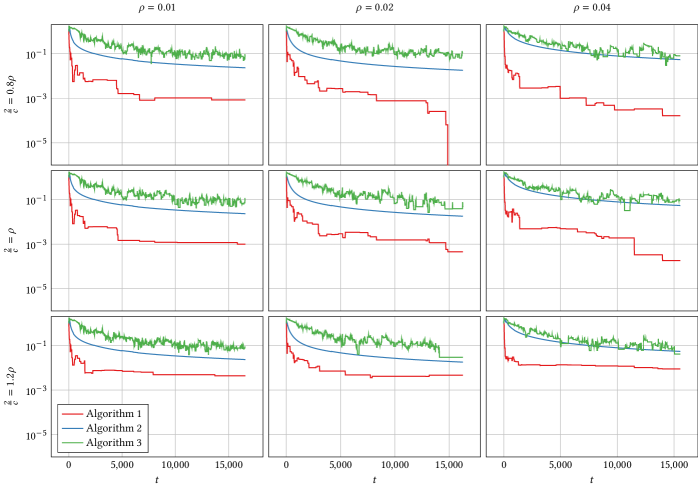
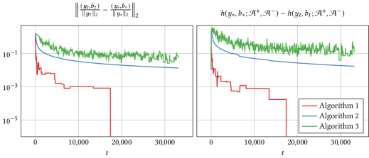
| Alg 1 | Alg 2 | Alg 3 | Alg 1 | Alg 2 | Alg 3 | Alg 1 | Alg 2 | Alg 3 | ||
| 250 | 9 | 37 | 37 | 9 | 28 | 35 | 9 | 31 | 32 | |
| 15000 | 9 | 308 | 985 | 9 | 130 | 861 | 9 | 319 | 631 | |
| 250 | 9 | 37 | 37 | 9 | 28 | 35 | 9 | 31 | 32 | |
| 15000 | 9 | 309 | 954 | 9 | 130 | 799 | 9 | 311 | 630 | |
| 250 | 9 | 37 | 37 | 9 | 28 | 35 | 9 | 31 | 32 | |
| 15000 | 9 | 310 | 1017 | 9 | 128 | 823 | 9 | 311 | 625 | |
| Alg 1 | Alg 2 | Alg 3 | Alg 1 | Alg 2 | Alg 3 | Alg 1 | Alg 2 | Alg 3 | ||
| 250 | 0 | 0 | 0 | 2 | 1 | 0 | 2 | 3 | 6 | |
| 15000 | 2 | 70 | 83 | 4 | 63 | 155 | 4 | 175 | 241 | |
| 250 | 0 | 1 | 0 | 2 | 3 | 0 | 3 | 5 | 6 | |
| 15000 | 9 | 96 | 102 | 13 | 81 | 184 | 15 | 243 | 312 | |
| 250 | 0 | 2 | 0 | 4 | 3 | 0 | 4 | 7 | 6 | |
| 15000 | 45 | 121 | 131 | 97 | 94 | 209 | 197 | 304 | 355 | |
| Alg 1 | Alg 2 | Alg 3 | Alg 1 | Alg 2 | Alg 3 | Alg 1 | Alg 2 | Alg 3 | ||
| 250 | 0.54 | 0.07 | 0.01 | 0.54 | 0.06 | 0.01 | 0.51 | 0.06 | 0.01 | |
| 15000 | 24.91 | 5.63 | 0.47 | 26.49 | 5.58 | 0.46 | 25.78 | 5.60 | 0.46 | |
| 250 | 0.54 | 0.07 | 0.01 | 0.54 | 0.05 | 0.01 | 0.51 | 0.05 | 0.01 | |
| 15000 | 24.93 | 5.59 | 0.47 | 26.66 | 5.56 | 0.47 | 26.57 | 5.59 | 0.47 | |
| 250 | 0.54 | 0.07 | 0.01 | 0.53 | 0.05 | 0.01 | 0.51 | 0.06 | 0.01 | |
| 15000 | 25.32 | 5.58 | 0.47 | 25.26 | 5.86 | 0.46 | 26.28 | 5.61 | 0.47 | |
References
- Ahmadi and Shanbhag [2014] Hesam Ahmadi and Uday V. Shanbhag. Data-driven first-order methods for misspecified convex optimization problems: Global convergence and rate estimates. In 53rd IEEE Conference on Decision and Control, pages 4228–4233, Los Angeles California USA, 2014. IEEE. doi: 10.1109/CDC.2014.7040048.
- Ahmadi et al. [2021] Saba Ahmadi, Hedyeh Beyhaghi, Avrim Blum, and Keziah Naggita. The strategic perceptron. In Proceedings of the 22nd ACM Conference on Economics and Computation, EC ’21, pages 6–25, New York, NY, USA, 2021. Association for Computing Machinery. ISBN 9781450385541. doi: 10.1145/3465456.3467629. URL https://doi.org/10.1145/3465456.3467629.
- Ahmadi et al. [2022] Saba Ahmadi, Hedyeh Beyhaghi, Avrim Blum, and Keziah Naggita. On Classification of Strategic Agents Who Can Both Game and Improve. In L. Elisa Celis, editor, 3rd Symposium on Foundations of Responsible Computing (FORC 2022), volume 218 of Leibniz International Proceedings in Informatics (LIPIcs), pages 3:1–3:22, Dagstuhl, Germany, 2022. Schloss Dagstuhl – Leibniz-Zentrum für Informatik. ISBN 978-3-95977-226-6. doi: 10.4230/LIPIcs.FORC.2022.3. URL https://drops-dev.dagstuhl.de/entities/document/10.4230/LIPIcs.FORC.2022.3.
- Ahmadi et al. [2023] Saba Ahmadi, Avrim Blum, and Kunhe Yang. Fundamental Bounds on Online Strategic Classification. In Proceedings of the 24th ACM Conference on Economics and Computation, pages 22–58, London United Kingdom, July 2023. ACM. ISBN 9798400701047. doi: 10.1145/3580507.3597818. URL https://dl.acm.org/doi/10.1145/3580507.3597818.
- Alon et al. [2020] Tal Alon, Magdalen Dobson, Ariel Procaccia, Inbal Talgam-Cohen, and Jamie Tucker-Foltz. Multiagent evaluation mechanisms. Proceedings of the AAAI Conference on Artificial Intelligence, 34(02):1774–1781, Apr. 2020. doi: 10.1609/aaai.v34i02.5543. URL https://ojs.aaai.org/index.php/AAAI/article/view/5543.
- Bechavod et al. [2021] Yahav Bechavod, Katrina Ligett, Steven Wu, and Juba Ziani. Gaming helps! learning from strategic interactions in natural dynamics. In Arindam Banerjee and Kenji Fukumizu, editors, Proceedings of The 24th International Conference on Artificial Intelligence and Statistics, volume 130 of Proceedings of Machine Learning Research, pages 1234–1242. PMLR, 13–15 Apr 2021. URL https://proceedings.mlr.press/v130/bechavod21a.html.
- Bechavod et al. [2022] Yahav Bechavod, Chara Podimata, Steven Wu, and Juba Ziani. Information discrepancy in strategic learning. In Kamalika Chaudhuri, Stefanie Jegelka, Le Song, Csaba Szepesvari, Gang Niu, and Sivan Sabato, editors, Proceedings of the 39th International Conference on Machine Learning, volume 162 of Proceedings of Machine Learning Research, pages 1691–1715. PMLR, 17–23 Jul 2022. URL https://proceedings.mlr.press/v162/bechavod22a.html.
- Braverman and Garg [2020] Mark Braverman and Sumegha Garg. The Role of Randomness and Noise in Strategic Classification. In Aaron Roth, editor, 1st Symposium on Foundations of Responsible Computing (FORC 2020), volume 156 of Leibniz International Proceedings in Informatics (LIPIcs), pages 9:1–9:20, Dagstuhl, Germany, 2020. Schloss Dagstuhl – Leibniz-Zentrum für Informatik. ISBN 978-3-95977-142-9. doi: 10.4230/LIPIcs.FORC.2020.9. URL https://drops-dev.dagstuhl.de/entities/document/10.4230/LIPIcs.FORC.2020.9.
- Brückner and Scheffer [2011] Michael Brückner and Tobias Scheffer. Stackelberg games for adversarial prediction problems. In Proceedings of the 17th ACM SIGKDD international conference on Knowledge discovery and data mining, pages 547–555, San Diego California USA, August 2011. ACM. ISBN 978-1-4503-0813-7. doi: 10.1145/2020408.2020495. URL https://dl.acm.org/doi/10.1145/2020408.2020495.
- Chen et al. [2018] Yiling Chen, Chara Podimata, Ariel D. Procaccia, and Nisarg Shah. Strategyproof linear regression in high dimensions. In Proceedings of the 2018 ACM Conference on Economics and Computation, EC ’18, pages 9–26, New York, NY, USA, 2018. Association for Computing Machinery. ISBN 9781450358293. doi: 10.1145/3219166.3219175. URL https://doi.org/10.1145/3219166.3219175.
- Chen et al. [2020] Yiling Chen, Yang Liu, and Chara Podimata. Learning strategy-aware linear classifiers. In Proceedings of the 34th International Conference on Neural Information Processing Systems, NIPS’20, Red Hook, NY, USA, 2020. Curran Associates Inc. ISBN 9781713829546.
- Dalvi et al. [2004] Nilesh Dalvi, Pedro Domingos, Mausam, Sumit Sanghai, and Deepak Verma. Adversarial classification. In Proceedings of the Tenth ACM SIGKDD International Conference on Knowledge Discovery and Data Mining, KDD ’04, pages 99–108, New York, NY, USA, 2004. Association for Computing Machinery. ISBN 1581138881. doi: 10.1145/1014052.1014066. URL https://doi.org/10.1145/1014052.1014066.
- Dekel et al. [2008] Ofer Dekel, Felix Fischer, and Ariel D. Procaccia. Incentive compatible regression learning. In Proceedings of the Nineteenth Annual ACM-SIAM Symposium on Discrete Algorithms, SODA ’08, pages 884–893, USA, 2008. Society for Industrial and Applied Mathematics.
- Dong et al. [2018] Jinshuo Dong, Aaron Roth, Zachary Schutzman, Bo Waggoner, and Zhiwei Steven Wu. Strategic Classification from Revealed Preferences. In Proceedings of the 2018 ACM Conference on Economics and Computation, pages 55–70, Ithaca NY USA, June 2018. ACM. ISBN 978-1-4503-5829-3. doi: 10.1145/3219166.3219193. URL https://dl.acm.org/doi/10.1145/3219166.3219193.
- Freund and Schapire [1999] Yoav Freund and Robert E. Schapire. Large margin classification using the perceptron algorithm. Mach. Learn., 37(3):277–296, dec 1999. ISSN 0885-6125. doi: 10.1023/A:1007662407062. URL https://doi.org/10.1023/A:1007662407062.
- Frieß et al. [1998] Thilo-Thomas Frieß, Nello Cristianini, and Colin Campbell. The kernel-adatron algorithm: A fast and simple learning procedure for support vector machines. In Proceedings of the Fifteenth International Conference on Machine Learning, ICML ’98, pages 188–196, San Francisco, CA, USA, 1998. Morgan Kaufmann Publishers Inc. ISBN 1558605568.
- Gentile [2002] Claudio Gentile. A new approximate maximal margin classification algorithm. J. Mach. Learn. Res., 2:213–242, mar 2002. ISSN 1532-4435.
- Ghalme et al. [2021] Ganesh Ghalme, Vineet Nair, Itay Eilat, Inbal Talgam-Cohen, and Nir Rosenfeld. Strategic classification in the dark. In Marina Meila and Tong Zhang, editors, Proceedings of the 38th International Conference on Machine Learning, volume 139 of Proceedings of Machine Learning Research, pages 3672–3681. PMLR, 18–24 Jul 2021. URL https://proceedings.mlr.press/v139/ghalme21a.html.
- Haghtalab et al. [2020] Nika Haghtalab, Nicole Immorlica, Brendan Lucier, and Jack Z. Wang. Maximizing Welfare with Incentive-Aware Evaluation Mechanisms. In Proceedings of the Twenty-Ninth International Joint Conference on Artificial Intelligence, pages 160–166, Yokohama, Japan, July 2020. International Joint Conferences on Artificial Intelligence Organization. ISBN 978-0-9992411-6-5. doi: 10.24963/ijcai.2020/23. URL https://www.ijcai.org/proceedings/2020/23.
- Hardt et al. [2016] Moritz Hardt, Nimrod Megiddo, Christos Papadimitriou, and Mary Wootters. Strategic Classification. In Proceedings of the 2016 ACM Conference on Innovations in Theoretical Computer Science, pages 111–122, Cambridge Massachusetts USA, January 2016. ACM. ISBN 978-1-4503-4057-1. doi: 10.1145/2840728.2840730. URL https://dl.acm.org/doi/10.1145/2840728.2840730.
- Hiriart-Urruty and Lemaréchal [2001] Jean-Baptiste Hiriart-Urruty and Claude Lemaréchal. Fundamentals of Convex Analysis. Springer Berlin Heidelberg, Berlin, Heidelberg, 2001. ISBN 978-3-540-42205-1 978-3-642-56468-0. doi: 10.1007/978-3-642-56468-0. URL http://link.springer.com/10.1007/978-3-642-56468-0.
- Ho-Nguyen and Kılınç-Karzan [2021] Nam Ho-Nguyen and Fatma Kılınç-Karzan. Dynamic data-driven estimation of nonparametric choice models. Operations Research, 69(4):1228–1239, 2021. doi: 10.1287/opre.2020.2077. URL https://doi.org/10.1287/opre.2020.2077.
- Hu et al. [2019] Lily Hu, Nicole Immorlica, and Jennifer Wortman Vaughan. The Disparate Effects of Strategic Manipulation. In Proceedings of the Conference on Fairness, Accountability, and Transparency, pages 259–268, Atlanta GA USA, January 2019. ACM. ISBN 978-1-4503-6125-5. doi: 10.1145/3287560.3287597. URL https://dl.acm.org/doi/10.1145/3287560.3287597.
- Jagadeesan et al. [2021] Meena Jagadeesan, Celestine Mendler-Dünner, and Moritz Hardt. Alternative microfoundations for strategic classification. In Marina Meila and Tong Zhang, editors, Proceedings of the 38th International Conference on Machine Learning, volume 139 of Proceedings of Machine Learning Research, pages 4687–4697. PMLR, 18–24 Jul 2021. URL https://proceedings.mlr.press/v139/jagadeesan21a.html.
- Kivinen et al. [2004] Jyrki Kivinen, Alexander J Smola, and Robert C Williamson. Online learning with kernels. IEEE transactions on signal processing, 52(8):2165–2176, 2004.
- Kleinberg and Raghavan [2020] Jon Kleinberg and Manish Raghavan. How Do Classifiers Induce Agents to Invest Effort Strategically? ACM Transactions on Economics and Computation, 8(4):1–23, November 2020. ISSN 2167-8375, 2167-8383. doi: 10.1145/3417742. URL https://dl.acm.org/doi/10.1145/3417742.
- Kowalczyk [2000] Adam Kowalczyk. Maximal Margin Perceptron. In Advances in Large-Margin Classifiers. The MIT Press, 09 2000. ISBN 9780262283977. doi: 10.7551/mitpress/1113.003.0009. URL https://doi.org/10.7551/mitpress/1113.003.0009.
- Lechner and Urner [2022] Tosca Lechner and Ruth Urner. Learning Losses for Strategic Classification. Proceedings of the AAAI Conference on Artificial Intelligence, 36(7):7337–7344, June 2022. ISSN 2374-3468, 2159-5399. doi: 10.1609/aaai.v36i7.20696. URL https://ojs.aaai.org/index.php/AAAI/article/view/20696.
- Levanon and Rosenfeld [2021] Sagi Levanon and Nir Rosenfeld. Strategic classification made practical. In Marina Meila and Tong Zhang, editors, Proceedings of the 38th International Conference on Machine Learning, volume 139 of Proceedings of Machine Learning Research, pages 6243–6253. PMLR, 18–24 Jul 2021. URL https://proceedings.mlr.press/v139/levanon21a.html.
- Li and Long [1999] Yi Li and Philip Long. The relaxed online maximum margin algorithm. In S. Solla, T. Leen, and K. Müller, editors, Advances in Neural Information Processing Systems, volume 12. MIT Press, 1999. URL https://proceedings.neurips.cc/paper_files/paper/1999/file/515ab26c135e92ed8bf3a594d67e4ade-Paper.pdf.
- Miller et al. [2020] John Miller, Smitha Milli, and Moritz Hardt. Strategic classification is causal modeling in disguise. In Hal Daumé III and Aarti Singh, editors, Proceedings of the 37th International Conference on Machine Learning, volume 119 of Proceedings of Machine Learning Research, pages 6917–6926. PMLR, 13–18 Jul 2020. URL https://proceedings.mlr.press/v119/miller20b.html.
- Milli et al. [2019] Smitha Milli, John Miller, Anca D. Dragan, and Moritz Hardt. The Social Cost of Strategic Classification. In Proceedings of the Conference on Fairness, Accountability, and Transparency, pages 230–239, Atlanta GA USA, January 2019. ACM. ISBN 978-1-4503-6125-5. doi: 10.1145/3287560.3287576. URL https://dl.acm.org/doi/10.1145/3287560.3287576.
- Mohri et al. [2012] Mehryar. Mohri, Afshin. Rostamizadeh, and Ameet. Talwalkar. Foundations of machine learning. Adaptive computation and machine learning series. MIT Press, Cambridge, MA, 2012. ISBN 0262305666.
- Novikoff [1962] Albert BJ Novikoff. On convergence proofs on perceptrons. In Proceedings of the Symposium on the Mathematical Theory of Automata, volume 12, pages 615–622. New York, NY, 1962.
- Perdomo et al. [2020] Juan Perdomo, Tijana Zrnic, Celestine Mendler-Dünner, and Moritz Hardt. Performative prediction. In Hal Daumé III and Aarti Singh, editors, Proceedings of the 37th International Conference on Machine Learning, volume 119 of Proceedings of Machine Learning Research, pages 7599–7609. PMLR, 13–18 Jul 2020. URL https://proceedings.mlr.press/v119/perdomo20a.html.
- Rockafellar and Wets [2009] R Tyrrell Rockafellar and Roger J-B Wets. Variational analysis, volume 317. Springer Science & Business Media, 2009.
- Rockafellar [1970] Ralph Tyrell Rockafellar. Convex Analysis. Princeton University Press, December 1970. ISBN 978-1-4008-7317-3. doi: 10.1515/9781400873173. URL https://www.degruyter.com/document/doi/10.1515/9781400873173/html.
- Rosenblatt [1958] Frank Rosenblatt. The perceptron: a probabilistic model for information storage and organization in the brain. Psychological review, 65(6):386, 1958.
- Shavit et al. [2020] Yonadav Shavit, Benjamin Edelman, and Brian Axelrod. Causal strategic linear regression. In Hal Daumé III and Aarti Singh, editors, Proceedings of the 37th International Conference on Machine Learning, volume 119 of Proceedings of Machine Learning Research, pages 8676–8686. PMLR, 13–18 Jul 2020. URL https://proceedings.mlr.press/v119/shavit20a.html.
- Sundaram et al. [2023] Ravi Sundaram, Anil Vullikanti, Haifeng Xu, and Fan Yao. Pac-learning for strategic classification. Journal of Machine Learning Research, 24(192):1–38, 2023. URL http://jmlr.org/papers/v24/21-1250.html.
- Tsirtsis et al. [2024] Stratis Tsirtsis, Behzad Tabibian, Moein Khajehnejad, Adish Singla, Bernhard Schölkopf, and Manuel Gomez-Rodriguez. Optimal decision making under strategic behavior. Management Science, 2024. doi: 10.1287/mnsc.2021.02567. URL https://doi.org/10.1287/mnsc.2021.02567.
- Zhang and Conitzer [2021] Hanrui Zhang and Vincent Conitzer. Incentive-aware pac learning. Proceedings of the AAAI Conference on Artificial Intelligence, 35(6):5797–5804, May 2021. doi: 10.1609/aaai.v35i6.16726. URL https://ojs.aaai.org/index.php/AAAI/article/view/16726.
- Zrnic et al. [2021] Tijana Zrnic, Eric Mazumdar, Shankar Sastry, and Michael Jordan. Who leads and who follows in strategic classification? In M. Ranzato, A. Beygelzimer, Y. Dauphin, P.S. Liang, and J. Wortman Vaughan, editors, Advances in Neural Information Processing Systems, volume 34, pages 15257–15269. Curran Associates, Inc., 2021. URL https://proceedings.neurips.cc/paper_files/paper/2021/file/812214fb8e7066bfa6e32c626c2c688b-Paper.pdf.
Appendix A Proofs of auxiliary results
Lemma 13.
The subdifferential set of the function has the following characterizations:
Proof of Lemma 13.
Fix . By definition of the subdifferential, we have
Let us define the set . First, for any and any , using and Hölder’s inequality we arrive at
and so implies .
Conversely, for any and any , from the subdifferential inequality we arrive at
As this holds for all , we conclude
As the right-hand side is a finite number, we must have . Note that whenever , we have . So, we conclude , and in this case we have . This implies , where the second inequality follows from and the last one from Hölder’s inequality. Thus, each inequality in this chain must hold as equality, and . Thus, we have shown implies .
To show the last equivalent expression, it suffices to notice that for . ∎
Lemma 14.
Suppose is a closed convex cone. Then, the map , i.e., the projection operation onto the cone is positively homogeneous. That is, for any ,
Proof of Lemma 14.
The stated relation clearly holds when as is a closed convex cone. So, we assume . By definition, the projection operation is given by
Thus, for any ,
where the second equation follows from the fact that and is a closed convex cone. ∎
Remark 3.
Note that under Assumption 2, the response and proxy data functions are invariant to positive scalings of a classifier. That is, consider the classifiers given by and such that for some . Then, for any point , we have and .
To see this, observe that
Then, the if conditions in and will be satisfied precisely at the same time for both of the classifiers. Moreover, by definition of in (9c) and as , we have under Assumption 2. Thus, we conclude that and hold as well.
Lemma 15.
Suppose Assumption 2 holds and is a closed convex cone. Given a sequence of points , let be the sequence of classifiers obtained from Algorithm 3 when we set . For the same sequence of points, let be the sequence of classifiers obtained from Algorithm 3 for a fixed . Then, , and for all .
Proof of Lemma 15.
To ease our notation, we let , , , , , and .
We will prove that , , and holds for all by induction. The base case holds as . Suppose by induction hypothesis that for some . Then, by Remark 3, we have and . Let be computed based on (15) for the classifier . Thus,
where the first equation follows by definition and the second equation follows from the induction hypothesis that , and applying Lemma 14. In order to justify the third equation, note that as and , we have
where the third equation follows from . ∎
Lemma 16.
If a norm is different to any positive multiple of , then there exists such that and , are not parallel.
Proof of Lemma 16.
Assume for contradiction that for any . Then, since is a singleton for any , we deduce that it is differentiable at any . Since is not a positive multiple of , the same must hold for the dual norm. Then, consider any such that , and let . The sets and must be different, therefore there exists such that but . We let be the point with the smaller -norm, and be the point with the larger -norm, i.e., we have and . In particular, this implies cannot be parallel, hence for . Therefore, we can define the following parameterized curve on the dual norm ball:
Then, we have , (as ) and is differentiable (as we have for any ), and holds for all . Next, define , then using we arrive at
Now, recall that holds for all , and thus for any , we have
where the inequality holds by the subgradient inequality applied to and the assumption that (recall that as for all ). Dividing both sides by and letting , we obtain . Since this holds for any , this contradicts
Thus, there must exist some such that . ∎
Appendix B Supplementary numerical results
B.1 Real data with noisy agent responses
In this appendix, we investigate performance of the algorithms when noise is added to the agent responses. While we do not have theory for this setting we investigate the tolerance/robustness of our algorithms when the agent responses that the learner observes contain noise, which reflects the real world where agents may not be purely rational or our observations of their responses may be imperfect. We assume that instead of the learner observing directly the agent’s response , they observe , where is i.i.d. Gaussian noise. Using the same dataset from Section 5, we tested the impact of having . Note that corresponds to the noiseless setting which was discussed in Section 5.
Distance to best margin classifier with noise.
Comparing Figures 3, 5 and 6, we observe that Algorithms 1 and 2 are more sensitive to noise . In particular, performance in terms of convergence to the classifier of Algorithm 1 drastically deteriorates as the noise increases to . This is expected because the noise means that the proxy data are no longer guaranteed to be separable, and in fact inseparability becomes more likely as the noise level increases. When inseparability occurs, problem () in Algorithm 1 will give a solution of resulting in a prediction of always. As a result, Algorithm 1 breaks down and does not provide any useful information about once the separability assumption is violated, e.g., when the noise level is of the same order as and is large relative to . In contrast, Algorithm 2 does not seem to encounter this issue even when data may be inseparable, and provides a reasonable estimate of . It shows notably better performance than Algorithm 3. In fact, Figure 5 shows that when , it behaves mostly the same as in the noiseless case. As further increases to , however, the performance of Algorithm 2 deteriorates slightly as well. Finally, Algorithm 3 seems to be robust to the noise, achieving roughly the same (yet not very good) performance as in the noiseless setting even for .
Number of mistakes with noise.
Figures 7, 9, 8 and 5 compare the performance of the algorithms with noise. In terms of number of mistakes, the performance of Algorithm 1 diminishes when the data and become inseparable as amounts to always predicting a label of for any data point. In the cases where the proxy data are still separable, Algorithm 1 remains the best and makes the fewest mistakes. Algorithms 2 and 3 are more robust to noise and inseparability. From Table 5 we see that as increases the performance degradation (in terms of number of mistakes) of Algorithm 3 appears to be very minor compared to the other two algorithms. That said, from Figures 8 and 9 we see that Algorithm 2 typically makes less mistakes than Algorithm 3 in all parameter and noise settings. The robustness of Algorithm 3 is somewhat unsurprising, since finite mistake bounds for non-separable data exist for the perceptron in the non-strategic setting. That said, the robustness of Algorithm 2 is somewhat surprising, and warrants further investigation in future work. One possible explanation is that, even when the proxy data are inseparable, may be updated in Algorithm 2, whereas Algorithm 1 will be stuck at .
Number of manipulations with noise.
In Figures 10, 12, 11 and 6, we compare the performance of the algorithms in terms of number of manipulations they induce under noise. Note that the results for Algorithm 1 are meaningful only when the dataset remains separable. Otherwise, no manipulation will happen once , but this is not really an indication of better performance. For Algorithms 2 and 3, we do not see drastic changes in the number of manipulations depending on the noise level, and in some cases there are even fewer manipulations when noise is present.
Solution times with noise.
Table 7 shows very similar performance across all three algorithms when compared to the noiseless case.
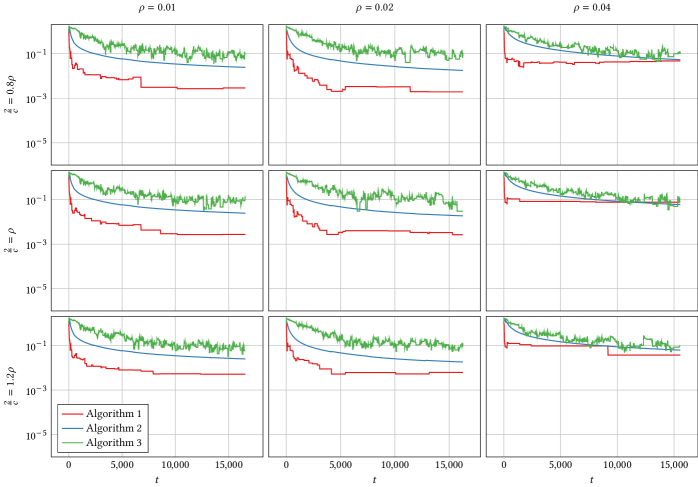
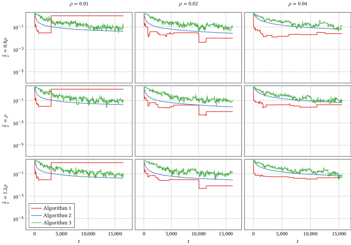
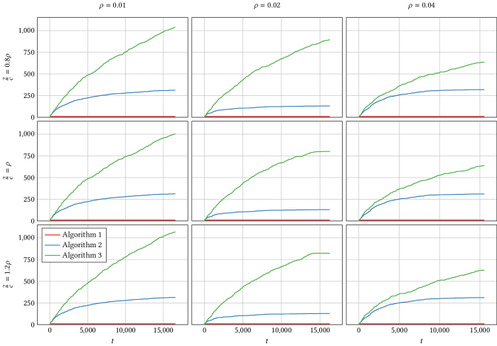
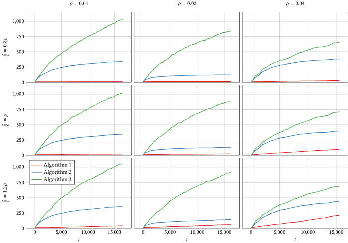
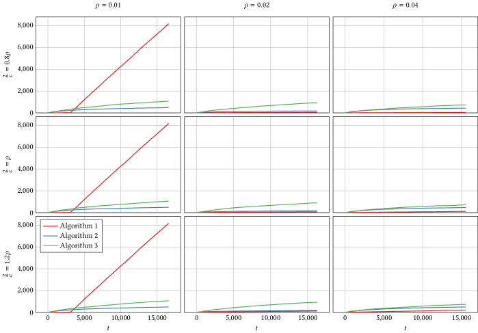
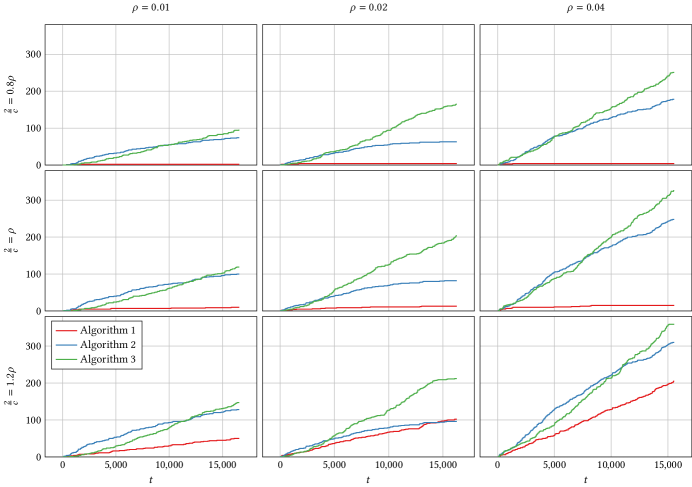
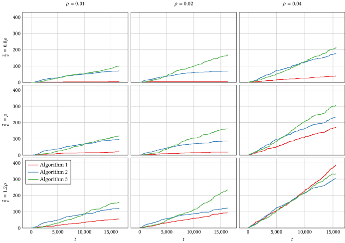
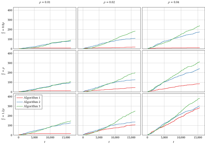
| Alg 1 | Alg 2 | Alg 3 | Alg 1 | Alg 2 | Alg 3 | Alg 1 | Alg 2 | Alg 3 | ||
| 250 | 9 | 37 | 37 | 9 | 28 | 35 | 9 | 31 | 32 | |
| 15000 | 9 | 308 | 985 | 9 | 130 | 861 | 9 | 319 | 631 | |
| 250 | 9 | 37 | 37 | 9 | 28 | 35 | 9 | 31 | 32 | |
| 15000 | 9 | 309 | 954 | 9 | 130 | 799 | 9 | 311 | 630 | |
| 250 | 9 | 37 | 37 | 9 | 28 | 35 | 9 | 31 | 32 | |
| 15000 | 9 | 310 | 1017 | 9 | 128 | 823 | 9 | 311 | 625 | |
| Alg 1 | Alg 2 | Alg 3 | Alg 1 | Alg 2 | Alg 3 | Alg 1 | Alg 2 | Alg 3 | ||
| 250 | 9 | 37 | 37 | 11 | 29 | 35 | 9 | 32 | 32 | |
| 15000 | 11 | 335 | 971 | 12 | 122 | 817 | 30 | 380 | 648 | |
| 250 | 9 | 36 | 37 | 11 | 29 | 35 | 9 | 31 | 33 | |
| 15000 | 18 | 339 | 966 | 21 | 128 | 860 | 94 | 396 | 706 | |
| 250 | 9 | 36 | 37 | 12 | 30 | 35 | 11 | 32 | 33 | |
| 15000 | 36 | 348 | 1006 | 57 | 138 | 883 | 206 | 439 | 686 | |
| Alg 1 | Alg 2 | Alg 3 | Alg 1 | Alg 2 | Alg 3 | Alg 1 | Alg 2 | Alg 3 | ||
| 250 | 8 | 37 | 39 | 15 | 30 | 35 | 10 | 32 | 33 | |
| 15000 | 7235 | 463 | 1007 | 53 | 176 | 895 | 39 | 430 | 724 | |
| 250 | 8 | 37 | 39 | 16 | 30 | 35 | 10 | 32 | 31 | |
| 15000 | 7236 | 470 | 991 | 72 | 172 | 866 | 108 | 463 | 703 | |
| 250 | 8 | 37 | 39 | 17 | 31 | 38 | 11 | 32 | 31 | |
| 15000 | 7238 | 475 | 1020 | 115 | 179 | 895 | 205 | 493 | 728 | |
| Alg 1 | Alg 2 | Alg 3 | Alg 1 | Alg 2 | Alg 3 | Alg 1 | Alg 2 | Alg 3 | ||
| 250 | 0 | 0 | 0 | 2 | 1 | 0 | 2 | 3 | 6 | |
| 15000 | 2 | 70 | 83 | 4 | 63 | 155 | 4 | 175 | 241 | |
| 250 | 0 | 1 | 0 | 2 | 3 | 0 | 3 | 5 | 6 | |
| 15000 | 9 | 96 | 102 | 13 | 81 | 184 | 15 | 243 | 312 | |
| 250 | 0 | 2 | 0 | 4 | 3 | 0 | 4 | 7 | 6 | |
| 15000 | 45 | 121 | 131 | 97 | 94 | 209 | 197 | 304 | 355 | |
| Alg 1 | Alg 2 | Alg 3 | Alg 1 | Alg 2 | Alg 3 | Alg 1 | Alg 2 | Alg 3 | ||
| 250 | 0 | 0 | 0 | 2 | 1 | 0 | 1 | 3 | 3 | |
| 15000 | 4 | 68 | 86 | 4 | 68 | 157 | 38 | 173 | 205 | |
| 250 | 0 | 1 | 0 | 2 | 1 | 0 | 1 | 5 | 4 | |
| 15000 | 18 | 92 | 108 | 19 | 85 | 156 | 166 | 229 | 300 | |
| 250 | 0 | 1 | 0 | 4 | 3 | 0 | 6 | 7 | 5 | |
| 15000 | 50 | 115 | 149 | 89 | 116 | 216 | 371 | 296 | 331 | |
| Alg 1 | Alg 2 | Alg 3 | Alg 1 | Alg 2 | Alg 3 | Alg 1 | Alg 2 | Alg 3 | ||
| 250 | 2 | 0 | 0 | 3 | 3 | 0 | 3 | 5 | 3 | |
| 15000 | 9 | 75 | 79 | 17 | 105 | 167 | 11 | 171 | 232 | |
| 250 | 3 | 0 | 0 | 4 | 4 | 0 | 3 | 6 | 3 | |
| 15000 | 13 | 88 | 93 | 43 | 123 | 186 | 84 | 234 | 305 | |
| 250 | 4 | 0 | 0 | 7 | 5 | 0 | 6 | 7 | 4 | |
| 15000 | 16 | 118 | 134 | 103 | 132 | 231 | 276 | 294 | 373 | |
| Alg 1 | Alg 2 | Alg 3 | Alg 1 | Alg 2 | Alg 3 | Alg 1 | Alg 2 | Alg 3 | ||
| 250 | 0.54 | 0.07 | 0.01 | 0.54 | 0.06 | 0.01 | 0.51 | 0.06 | 0.01 | |
| 15000 | 24.91 | 5.63 | 0.47 | 26.49 | 5.58 | 0.46 | 25.78 | 5.60 | 0.46 | |
| 250 | 0.54 | 0.07 | 0.01 | 0.54 | 0.05 | 0.01 | 0.51 | 0.05 | 0.01 | |
| 15000 | 24.93 | 5.59 | 0.47 | 26.66 | 5.56 | 0.47 | 26.57 | 5.59 | 0.47 | |
| 250 | 0.54 | 0.07 | 0.01 | 0.53 | 0.05 | 0.01 | 0.51 | 0.06 | 0.01 | |
| 15000 | 25.32 | 5.58 | 0.47 | 25.26 | 5.86 | 0.46 | 26.28 | 5.61 | 0.47 | |
| Alg 1 | Alg 2 | Alg 3 | Alg 1 | Alg 2 | Alg 3 | Alg 1 | Alg 2 | Alg 3 | ||
| 250 | 0.53 | 0.07 | 0.01 | 0.53 | 0.05 | 0.01 | 0.51 | 0.05 | 0.01 | |
| 15000 | 25.71 | 5.59 | 0.47 | 25.78 | 5.61 | 0.47 | 27.94 | 5.65 | 0.47 | |
| 250 | 0.53 | 0.07 | 0.01 | 0.52 | 0.05 | 0.01 | 0.54 | 0.05 | 0.01 | |
| 15000 | 25.28 | 5.71 | 0.47 | 26.07 | 5.57 | 0.47 | 24.4 | 5.60 | 0.48 | |
| 250 | 0.53 | 0.07 | 0.01 | 0.52 | 0.05 | 0.01 | 0.52 | 0.05 | 0.01 | |
| 15000 | 25.34 | 5.57 | 0.47 | 24.65 | 5.49 | 0.47 | 24.21 | 5.67 | 0.47 | |
| Alg 1 | Alg 2 | Alg 3 | Alg 1 | Alg 2 | Alg 3 | Alg 1 | Alg 2 | Alg 3 | ||
| 250 | 0.50 | 0.07 | 0.01 | 0.55 | 0.05 | 0.01 | 0.50 | 0.05 | 0.01 | |
| 15000 | 23.73 | 5.57 | 0.47 | 24.97 | 5.45 | 0.47 | 26.53 | 5.60 | 0.47 | |
| 250 | 0.49 | 0.07 | 0.01 | 0.55 | 0.05 | 0.01 | 0.50 | 0.05 | 0.01 | |
| 15000 | 23.83 | 5.53 | 0.47 | 25.01 | 5.61 | 0.46 | 25.86 | 5.55 | 0.48 | |
| 250 | 0.49 | 0.07 | 0.01 | 0.54 | 0.05 | 0.01 | 0.50 | 0.06 | 0.01 | |
| 15000 | 24.18 | 5.64 | 0.47 | 24.86 | 5.56 | 0.46 | 26.74 | 5.56 | 0.48 | |
B.2 Numerical results on synthetic data
In this section, we explore a synthetic dataset different from the loan dataset considered in Section 5. Here, feature vectors are generated by the truncated normal distribution on with mean and covariance . Labels are designated using a predefined classifier , , i.e., . Similar to the preprocessing procedure in Section 5, we remove the points that are within a distance of to the hyperplane defined by to create a strictly positive margin. We also follow the same process outlined in Section 5 to compute the best margin classifier . Then, the data are translated by where are computed from Lemma 5 (see its proof for an explicit expression using the primal and dual variables of the margin maximization problem, which can be retrieved from the MOSEK solver) so that the best margin classifier of the resulting data becomes . In this way, we can implement and test the performance of Algorithm 3 with . We mention that this in fact makes the task more challenging for Algorithms 1 and 2, as they do not have access to the information and need to figure it out via the mechanism of the algorithms themselves. However, as we will see in the numerical results, Algorithms 1 and 2 still have better performance in spite of this disadvantage. We do not add agent response noise for our synthetic experiments. The numerical results for the synthetic data are shown in Figures 13, 15, 14, 8, 9 and 10. Our observations here are consistent with the ones for the real data in terms of performance comparison among the three algorithms. On the other hand, in the synthetic data experiments the performance of Algorithm 2, in terms of both convergence to and number of mistakes, seems to improve and approach to that of Algorithm 1 in some parameter settings. Also, in almost all parameter combinations tested, the number of mistakes made by any algorithm is lower than that of loan data experiments and they all seem to stabilize after certain number of iterations, unlike the loan data experiments in which only Algorithm 1 seems stabilize within the finitely many iterations tested.
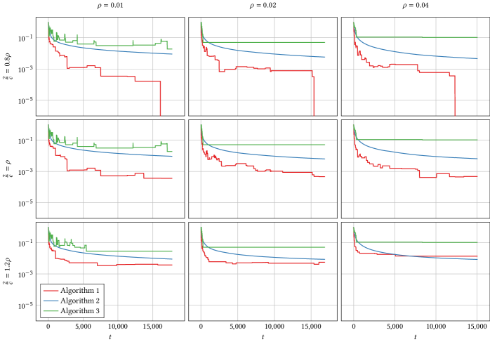
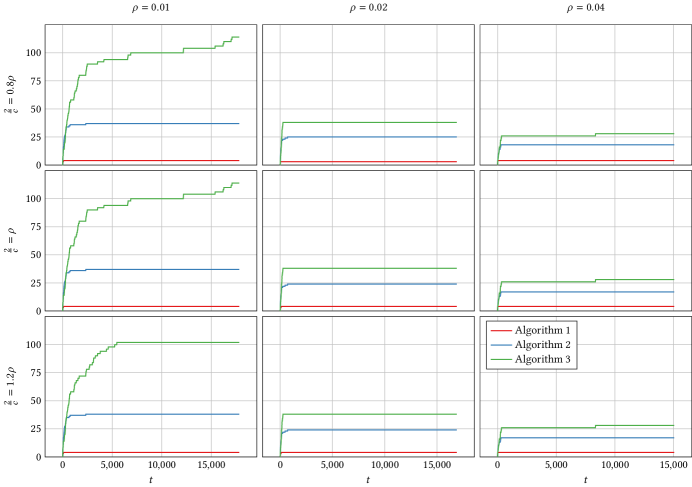
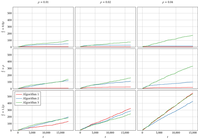
| Alg 1 | Alg 2 | Alg 3 | Alg 1 | Alg 2 | Alg 3 | Alg 1 | Alg 2 | Alg 3 | ||
| 250 | 4 | 27 | 22 | 3 | 23 | 36 | 4 | 16 | 22 | |
| 15000 | 4 | 37 | 104 | 3 | 25 | 38 | 4 | 18 | 28 | |
| 250 | 4 | 27 | 22 | 4 | 22 | 36 | 4 | 14 | 22 | |
| 15000 | 4 | 37 | 104 | 4 | 24 | 38 | 4 | 17 | 28 | |
| 250 | 4 | 28 | 22 | 4 | 22 | 36 | 4 | 14 | 22 | |
| 15000 | 4 | 38 | 102 | 4 | 24 | 38 | 4 | 17 | 28 | |
| Alg 1 | Alg 2 | Alg 3 | Alg 1 | Alg 2 | Alg 3 | Alg 1 | Alg 2 | Alg 3 | ||
| 250 | 5 | 4 | 4 | 3 | 9 | 9 | 5 | 10 | 10 | |
| 15000 | 6 | 44 | 74 | 4 | 28 | 68 | 5 | 18 | 173 | |
| 250 | 5 | 5 | 4 | 6 | 11 | 12 | 6 | 12 | 11 | |
| 15000 | 10 | 107 | 105 | 25 | 103 | 143 | 20 | 99 | 332 | |
| 250 | 8 | 6 | 5 | 9 | 11 | 13 | 10 | 16 | 15 | |
| 15000 | 106 | 164 | 162 | 291 | 259 | 214 | 547 | 425 | 534 | |
| Alg 1 | Alg 2 | Alg 3 | Alg 1 | Alg 2 | Alg 3 | Alg 1 | Alg 2 | Alg 3 | ||
| 250 | 0.58 | 0.06 | 0.01 | 0.61 | 0.06 | 0.01 | 0.56 | 0.06 | 0.01 | |
| 15000 | 24.86 | 5.56 | 0.45 | 25.42 | 5.52 | 0.44 | 25.31 | 5.70 | 0.44 | |
| 250 | 0.58 | 0.06 | 0.01 | 0.58 | 0.05 | 0.01 | 0.53 | 0.05 | 0.01 | |
| 15000 | 25.29 | 5.52 | 0.45 | 25.88 | 5.50 | 0.44 | 25.81 | 5.51 | 0.44 | |
| 250 | 0.60 | 0.06 | 0.01 | 0.61 | 0.05 | 0.01 | 0.53 | 0.05 | 0.01 | |
| 15000 | 25.08 | 5.75 | 0.44 | 24.64 | 5.71 | 0.44 | 24.37 | 5.45 | 0.44 | |