Incentive-Compatible Vertiport Reservation in Advanced
Air Mobility: An Auction-Based Approach

Abstract

The rise of advanced air mobility (AAM) is expected to become a multibillion-dollar industry in the near future. Market-based mechanisms are touted to be an integral part of AAM operations, which comprise heterogeneous operators with private valuations. In this work, we study the problem of designing a mechanism to coordinate the movement of electric vertical take-off and landing (eVTOL) aircraft, operated by multiple operators each having heterogeneous valuations associated with their fleet, between vertiports, while enforcing the arrival, departure, and parking constraints at vertiports. Particularly, we propose an incentive-compatible and individually rational vertiport reservation mechanism that maximizes a social welfare metric, which encapsulates the objective of maximizing the overall valuations of all operators while minimizing the congestion at vertiports. Additionally, we improve the computational tractability of designing the reservation mechanism by proposing a mixed binary linear programming approach that is based on constructing network flow graph corresponding to the underlying problem.

1 Introduction

Advanced air mobility (AAM) encompasses the utilization of unmanned aerial vehicles (UAVs), air taxis, and various cargo and passenger transport solutions. This innovative approach taps into previously unexplored airspace, poised to revolutionize urban airspace. A recent report forecasts the air mobility market alone to exceed US$50 billion by 2035, underlining this area’s immense growth potential (Cohen et al., 2021).

Despite the widespread optimism surrounding AAM, the design of regulatory policies remains an open problem. While ideas from conventional air traffic framework could be leveraged (Bertsimas and Patterson, 1998, 2000; Bertsimas et al., 2011; Roy and Tomlin, 2007; Odoni, 1987), they often fall short in accommodating the dynamic and adaptable nature of AAM operations (Bichler et al., 2023). Unlike traditional aviation, AAM requires a more flexible regulatory approach to be able to handle on-demand operations comprising of broader spectrum of arrival and departure points (Skorup, 2019; Seuken et al., 2022).

Administrative management methods prevalent in conventional airspace, such as grand-fathering rights, flow management, and first-come-first-serve, prove ineffective for AAM operations (Guerreiro et al., ; Evans et al., ). These approaches fail to elicit the heterogeneous private valuations (arising from different aircraft specifications, demand realization, etc.) different operators have on using AAM resources. Furthermore, they risk fostering inefficient and anti-competitive outcomes, as evidenced in traditional airspace operations (Dixit et al., 2023). Recognizing the need for tailored regulation, the Federal Aviation Administration (FAA) is actively developing a clean-slate congestion management framework for AAM operations to ensure efficiency, fairness, and safety (Administration, 2023).

Market-based congestion management mechanisms have been proposed as potential solutions for AAM operations (Chin et al., 2023b; Qin and Balakrishnan, 2022; Wang et al., 2023; Evans et al., ; Skorup, 2019; Seuken et al., 2022). In this paper, we study an auction-based mechanism for AAM congestion management.

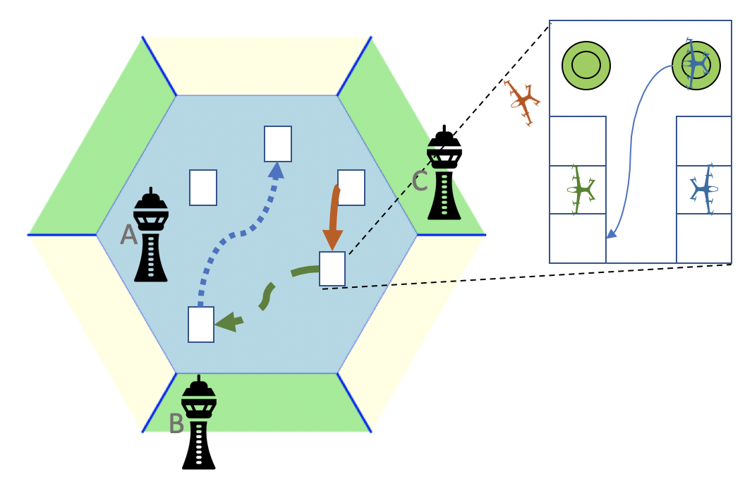
Figure 1: Schematic representation of the air traffic network with multiple service providers, each operating in non-overlapping operation regime, tasked with coordinating the movement of aircraft of various fleet operators between vertiports in its domain. Each vertiport has a constraint on the number of arriving aircraft, departing aircraft, and parked aircraft.

Even in conventional airspace management, auction-based mechanisms are extensively studied such as (Ball et al., 2018; Basso and Zhang, 2010; Carlin and Park, 1970; Mehta and Vazirani, 2020), where both theoretical and empirical evidence show their precedence over administrative approaches (Dixit et al., 2023). Despite being a plausible direction, auctioning airspace is rarely adopted in conventional airspace due to intricate and inflexible government regulations in conventional airspace operations (Bichler et al., 2023).

The design of market-based mechanisms that guarantee safety, efficiency, and fairness under the heterogeneous and on-demand nature of AAM operations has remained elusive. Particularly, there are two challenges. First, there are computational challenges associated with computing the auction mechanism. Second, there are challenges to truthfully elicit private information (aka incentive compatibility) from AAM operators. Existing approaches in AAM operations concentrate heavily on tactical deconfliction (Kleinbekman et al., 2018; Bertram and Wei, ), while strategic trajectories are determined through flow management frameworks or other protocols which do not account for economic incentives (Chin et al., 2021; Sun et al., 2023; Chin et al., 2023a, b; Wang et al., 2023; Qin and Balakrishnan, 2022; Guerreiro et al., ; Evans et al., ). Facing these issues, we propose a vertiport reservation mechanism, based on auction theory, that can be integrated into the airborne automation workflow proposed in (Wei et al., 2023). Particularly, the main motivating question in this work is as follows.

How do we design an incentive-compatible vertiport reservation mechanism that can accommodate the heterogeneous nature of AAM operations, while having good computational performance?

A schematic representation of vertiport reservation problem is presented in Figure 1. Typically, the air transportation network (ATN) for eVTOL aircraft is envisioned to be divided into several contiguous regions, each operated by a service provider (SP) (Skorup, 2019). In this work, we focus on one region of ATN which is managed by a SP, who is responsible for ensuring the efficient, safe, and fair movement of aircraft between various vertiports. The aircraft are owned by fleet operators (FOs), and each FO may own multiple aircraft. Each FO submits a menu of routes for each of its aircraft to SP, for each of which it has private valuation. The SP is then responsible for allocating different aircraft to routes.

The goal of the SP is to maximize a metric of social welfare that is comprised of two objectives: $(i)$ maximizing the overall (weighted) valuations of all FOs, and $(ii)$ minimizing excessive congestion at vertiports. Additionally, the SP must $(iii)$ ensure safety by enforcing arrival, departure, and parking capacity constraints at vertiports, and $(iv)$ elicit truthful valuations from heterogeneous FOs in the form of bids. We emphasize that this problem is an “exchange problem”, where some of the resources desired by any FO could be occupied by aircraft of FOs, and a feasible allocation in this setting needs to exchange the resources between FOs while respecting capacity constraints. In contrast, the standard slot allocation problems studied in conventional air traffic literature (cf. (Dixit et al., 2023; Mehta and Vazirani, 2020; Ball et al., 2018; Rassenti et al., 1982; Pertuiset and Santos, 2014; Ball et al., 2020; Bichler et al., 2023)) are “assignment problems” where the slots need to be assigned to airlines and not exchanged between airlines.

In this work, we propose an auction mechanism for the SP that satisfies $(i)-(iv)$. In our proposed mechanism, using the bids submitted by FOs, the SP allocates the resources by maximizing social welfare, subject to constraints. Additionally, we propose a payment mechanism, inspired by the generalized Vickrey–Clarke–Groves (VCG) mechanism (Nisan et al., 2007), that ensures that bids reveal true valuations of FOs. Specifically, each FO is charged a payment based on the externality imposed by them. Externality imposed by any FO is assessed by the difference in the optimal social welfare of remaining FOs when this FO is present versus when it is excluded from the auction environment. We theoretically study properties of the proposed mechanism in terms of incentive compatibility, individual rationality, and social welfare maximization (cf. Theorem 3.3).

There are two computational challenges associated with designing the auction mechanism. First, naively optimizing social welfare over the set of feasible allocations could be computationally challenging. Therefore, we frame the problem as a mixed integer linear program which is further converted to a mixed binary linear program by constructing a network-flow graph which consists of reduced number of discrete variables. Second, the computation of externality for the payment mechanism requires characterizing the set of feasible allocations when an FO is excluded from the auction environment, which is non-trivial as the underlying resource allocation problem is an exchange problem. Therefore, we introduce the idea of pseudo-bids, where we simply set a bid of $0$ to an FO while computing the optimal allocation when this FO is excluded from the auction environment.

Notation: We denote the set of real numbers by $\mathbb{R}$, non-negative real numbers by $\mathbb{R}_{+}$, integers by $\mathbb{Z}$, non-negative integers by $\mathbb{Z}_{+}$, and natural numbers by $\mathbb{N}$. For $N\in\mathbb{N}$, we define $[N]:=\{1,2,...,N\}$. The indicator function is denoted as $\mathbf{1}(\cdot)$, which is 1 when $(\cdot)$ is true and 0 otherwise. When indexing a vector $b=(b_{1},b_{2},...,b_{N})$, we follow the standard game-theoretic notation: $b_{-i}:=(b_{1},...,b_{i-1},b_{i+1},...,b_{N})$.

A table containing all major notations used in this article is presented in Appendix A.

2 Problem Setup

2.1 System Model

2.1.1 High-level description of model:

We examine an air transportation network (ATN) comprising multiple vertiports, catering to electric vertical take-off and landing (eVTOL) fleet operators, each operating multiple eVTOL aircraft. Our focus lies on a strategic deconfliction mechanism, complementing the tactical deconfliction algorithms proposed in prior works [(Kleinbekman et al., 2018; Wu et al., 2022; Bertram and Wei, ; Shao et al., 2021)]. We tackle the challenge of efficiently coordinating the arrival and departure of aircraft on the ATN, over a finite time window, by soliciting valuations from fleet operators in the form of bids, while ensuring all operational constraints are met.

At the onset of each time window, every fleet operator (FO) submits a comprehensive “menu” of ”routes” — a detailed list comprising origin-destination pairs along with departure and arrival times for each aircraft in their fleet. Concurrently, for each route in the menu, they include corresponding bids indicating the amount they are willing to pay should their aircraft be allocated that specific route. Subsequently, the service provider (SP) undertakes the task of computing a feasible allocation and corresponding payments, executing them seamlessly throughout the time window. With allocations finalized, granted aircraft are free to proceed to their desired destinations.

In situations where vertiports face congestion, reaching full parking capacity, any additional arrivals trigger the simultaneous departure of an aircraft from that vertiport. This dynamic transforms the problem into an “exchange problem” rather than the conventional “assignment problem” typically encountered in other air traffic allocation scenarios (Dixit et al., 2023; Mehta and Vazirani, 2020; Ball et al., 2018; Rassenti et al., 1982; Pertuiset and Santos, 2014; Ball et al., 2020; Bichler et al., 2023).

2.1.2 Detailed description of model:

We denote the set of vertiports by $R$, the set of FOs by $F$, and the set of eVTOL aircraft by $A$. We consider the problem of scheduling aircraft to and from vertiports over a time window of $H$ time slots.

Vertiports

At any time $t\in[H]$, each vertiport $r\in R$ has three kind of capacity constraints: (i) arrival capacity constraints, denoted by $\textsf{arr}(r,t)\in\mathbb{Z}_{+}$, that restrict the number of eVTOLs that can land at vertiport $r$ at time $t$; (ii) departure capacity constraints, denoted by $\textsf{dep}(r,t)\in\mathbb{Z}_{+}$, that restrict the number of eVTOLs that can depart from vertiport $r$ at time $t$; (iii) parking capacity constraints, denoted by $\textsf{park}(r,t)\in\mathbb{Z}_{+}$, that restrict the number of eVTOLs that can park at vertiport $r$ at time $t$.

Fleet Operators

Let $A_{i}$ be the fleet of aircraft operated by FO $i\in F$, and $A:=\{a_{i,j}|i\in F,j\in A_{i}\}$ be the set of all aircraft using the ATN. Each aircraft $a_{i,j}$ is identified by the following tuple

$$a_{i,j}\equiv\left(r^{\textsf{orig}}_{i,j},m_{i,j},\{t^{\textsf{dep}}_{i,j,k},t^{\textsf{arr}}_{i,j,k},v_{i,j,k},b_{i,j,k},r^{\textsf{dest}}_{i,j,k}\}_{k\in m_{i,j}}\right),$$ (Aircraft)

where $(i)$ $r^{\textsf{orig}}_{i,j}\in R$ is the origin vertiport of aircraft $a_{i,j}$, $(ii)$ $m_{i,j}$ is the menu of available routes to aircraft $a_{i,j}$; $(iii)$ any route $k\in m_{i,j}$ implies that aircraft $a_{i,j}$ departs from $r^{\textsf{orig}}_{i,j}\in R$ at time $t^{\textsf{dep}}_{i,j,k}$ to arrive at $r^{\textsf{dest}}_{i,j,k}\in R$ at time $t^{\textsf{arr}}_{i,j,k}$; $(iv)$ $v_{i,j,k}$ denotes the private valuation of aircraft $a_{i,j}$ to choose the route $k\in m_{i,j}$; and $(v)$ $b_{i,j,k}\in\mathbb{R}_{+}$ is the bid submitted by FO $i$ to schedule aircraft $a_{i,j}$ on route $k\in m_{i,j}$. For concise notation, we define $L:=\sum_{i\in F}\sum_{j\in A_{i}}|m_{i,j}|$ to be the number of all possible routes, $L_{i}:=\sum_{j\in A_{i}}|m_{i,j}|$ to be the number of routes available to fleet operator $i\in F$, and $L_{-i}:=\sum_{\ell\in F\backslash\{i\}}\sum_{j\in A_{\ell}}|m_{\ell,j}|$ to be the number of routes available to fleet operators except $i$.

Additionally, for concise notation, we denote the joint bid profile of all aircraft operated by FO $i\in F$ by $B_{i}:=(b_{i,j,k})_{j\in A_{i},k\in m_{i,j}}$ and joint valuation profile of its fleet by $V_{i}:=(v_{i,j,k})_{j\in A_{i},k\in m_{i,j}}$. For succinct notation, we denote the joint bid and valuation profile of all FOs as $B:=(B_{i})_{i\in F}$ and $V:=(V_{i})_{i\in F}$, respectively.

2.2 Problem Formulation

We consider an SP tasked with coordinating the movement of aircraft by allocating them to their desired vertiports while ensuring that the capacity constraints are met. Formally, the SP needs to decide on a feasible allocation ${x}=({x}_{i,j,k}\in\{0,1\}|i\in F,j\in A_{i},k\in m_{i,j})$, where

$${x}_{i,j,k}=\begin{cases}1,&\text{if aircraft $a_{i,j}$ is allocated route $k\in m_{i,j}$,}\\ 0,&\text{otherwise}.\end{cases}$$

Given an allocation ${x}$, let $S(r,t,{x})\in\mathbb{Z}_{+}$ denote the state of vertiport – defined to be the number of aircraft occupying the parking spots at vertiport $r\in R$ at time $t\in[H]$. For every $r\in R$, the initial occupation $S(r,1,{x})$ is defined as

$$S(r,1,x):=\sum_{i\in F}\sum_{j\in A_{i}}\mathbf{1}(r^{\textsf{orig}}_{i,j}=r).$$

For concise notation, we shall denote $S(r,1,x)$ by $\bar{S}(r)$ for every $r\in R$ as it does not depend on $x$. Naturally, it must hold that, for every $r\in R,t\in\{2,\ldots,H\}$,

$$S(r,t,x) =S(r,t-1,x)+\sum_{i\in F}\sum_{j\in A_{i}}\sum_{k\in m_{i,j}}{x}_{i,j,k}\mathbf{1}(r^{\textsf{dest}}_{i,j,k}=r,t^{\textsf{arr}}_{i,j,k}=t)$$ (1)

$$\quad-\sum_{i\in F}\sum_{j\in A_{i}}\sum_{k\in m_{i,j}}{x}_{i,j,k}\mathbf{1}(r^{\textsf{orig}}_{i,j}=r,t^{\textsf{dep}}_{i,j,k}=t),$$

where the second (resp. third) term on the RHS in the above equation denotes the set of incoming (resp. departing) aircraft in vertiport $r$ at time $t$. The residual capacity at vertiport $r\in R$ at time $t\in[H]$ is $Z(r,t,{x}):=\textsf{park}(r,t)-S(r,t,{x})$. To ensure the existence of a feasible allocation as defined later in (2), we assume that $\textsf{park}(r,t)-\bar{S}(r)\geq 0,\forall r\in R,t\in[H]$.

An allocation $x$ is called feasible if it satisfies the following constraints:

• Each aircraft is allocated at most one route. That is, for every $i\in F,j\in A_{i}$,

  $$\sum_{k\in m_{i,j}}{x}_{i,j,k}\leq 1.$$

• Arrival and departure capacity constraints must be satisfied at every vertiport $r$ at all times. That is, for every $r\in R,t\in[H]$,

  $$\sum_{i\in F}\sum_{j\in A_{i}}\sum_{k\in m_{i,j}}{x}_{i,j,k}\mathbf{1}(r^{\textsf{dest}}_{i,j,k}=r,t^{\textsf{arr}}_{i,j,k}=t)\leq\textsf{arr}(r,t),$$

  $$\sum_{i\in F}\sum_{j\in A_{i}}\sum_{k\in m_{i,j}}{x}_{i,j,k}\mathbf{1}(r^{\textsf{orig}}_{i,j}=r,t^{\textsf{dep}}_{i,j,k}=t)\leq\textsf{dep}(r,t).$$

• Parking capacity constraints must be satisfied. That is, for every vertiport $r\in R$ at any time $t\in[H]$, $Z(r,t,x)\geq 0$.

Consequently, the set of feasible allocation is defined as

$$X:=\left\{{x}\in\{0,1\}^{L}\Big{|}~{}\text{${x}$ satisfies (C1)-(C3)}\right\}.$$ (2)

Definition 2.1 (Social Welfare).

The social welfare of any allocation $x\in X$ is defined as follows.

$$\textsf{SW}({x};V):=\sum\limits_{i\in F}\rho_{i}\sum\limits_{j\in A_{i}}\sum\limits_{k\in m_{i,j}}v_{i,j,k}\cdot{x}_{i,j,k}-\lambda\sum\limits_{r\in R}\sum\limits_{t\in[H]}C_{r,t}(S(r,t,x)),$$ (3)

where $(i)$ $\rho_{i}\in\mathbb{R}_{+}$ is the weight factor specifying the relative importance of different FOs, $(ii)$ $C_{r,t}:\mathbb{Z}_{+}\rightarrow\mathbb{R}_{+}$ with $C_{r,t}(0)=0$ is discrete convex to capture increasing marginal cost of congestion, and $(iii)~{}\lambda\in\mathbb{R}_{+}$ is the ratio between the congestion cost and the cumulative weighted valuations of FOs. Furthermore, we define an optimal allocation as

$${x}^{\ast}(V)\in\underset{{x}\in X}{\arg\max}\ \textsf{SW}({x};V),$$ (4)

where ties are resolved arbitrarily.

Remark 2.2.

The social welfare objective (3) captures three main desiderata: efficiency, fairness, and safety. The objective (3) incorporates efficiency through additive valuations of FOs. Additionally, it incorporates the proportional fairness criterion by assigning different weights to the valuations of different FOs, denoted by $(\rho_{i})_{i\in F}$. Well-constructed weights can prevent larger FOs from monopolizing the resources. Finally, it encompasses safety considerations in two ways: first, through capacity constraints; and second, by introducing a congestion-dependent term in (3) that penalizes vertiports when the number of aircraft increases. With these three considerations, the definition of social welfare aligns closely with that presented in (Dixit et al., 2023).

We assume the SP does not have access to the true valuations $V$, as it is private information. Instead, the SP must use bids $B$ reported by the FOs to allocate the aircraft to vertiports through an auction mechanism – vertiport reservation mechanism. More formally, given a bid profile $B$, the SP uses a mechanism $\bar{M}=(\bar{{x}},(\bar{p}_{i})_{i\in F})$, where for a given bid profile $B$, $(i)$ $\bar{{x}}(B)\in X$ is the allocation proposed by the mechanism; and $(ii)$ $\bar{p}_{i}(B)\in\mathbb{R}$ denotes the payment charged to FO $i\in F$. Under the mechanism $\bar{M}$, the utility derived by any FO $i\in F$ is

$$U_{i}(B;\bar{M}):=\sum_{j\in A_{i}}\sum_{k\in m_{i,j}}v_{i,j,k}\textbf{1}(\bar{{x}}_{i,j,k}(B))-\bar{p}_{i}(B).$$ (5)

Given any arbitrary valuation profile $V$, the goal is to design a vertiport reservation mechanism $\bar{M}=(\bar{{x}},\bar{p})$ with the following desiderata.

• Incentive Compatibility (IC): Bidding truthfully is each FO’s (weakly) dominant strategy, i.e., for every $i\in F$, $B_{-i}\in\mathbb{R}_{+}^{L_{-i}}$,

  $$V_{i}\in\underset{B_{i}\in\mathbb{R}_{+}^{L_{i}}}{\arg\max}~{}U_{i}(B_{i},B_{-i};\bar{M}).$$

• Individual Rationality (IR): Bidding truthfully results in non-negative utility, i.e., for every $i\in F$,

  $$U_{i}(V_{i},B_{-i};\bar{M})\geq 0,\quad\forall\ B_{-i}\in\mathbb{R}_{+}^{L_{-i}}.$$

• Social Welfare Maximization (SWM): The resulting allocation maximizes social welfare, i.e.,

  $$\bar{{x}}(B)\in\underset{{x}\in X}{\arg\max}~{}\textsf{SW}({x};V).$$

3 Mechanism Design

We present an auction mechanism that satisfies (D1)-(D3) in Section 3.1, and prove its theoretical properties in Section 3.2. Moreover, we present an approach for computing the auction mechanism in Section 4.

3.1 Mechanism

Inspired by Myerson’s lemma (Myerson, 1981), our approach is to separate the allocation and payment functions so that the latter can ensure IC and IR as long as the former ensures maximization of total welfare in terms of bids submitted.

Allocation Function: Given a bid profile $B\in\mathbb{R}^{L}_{+}$, the allocation is obtained by

$$\bar{x}(B)\in\underset{{x}\in X}{\arg\max}~{}\textsf{SW}({x};B).$$ (6)

Payment Function: We first define a function $\theta:F\times\mathbb{R}_{+}^{L}\rightarrow\mathbb{R}_{+}^{L}$ such that for any $i\in F,j\in A_{i},k\in m_{i,j},$

$$\forall~{}\ell\in F,B\in\mathbb{R}_{+}^{L},\quad\theta_{i,j,k}(\ell,B)=\begin{cases}b_{i,j,k},&\text{if}\ i\neq\ell,\\ 0,&\text{if}\ i=\ell.\end{cases}$$ (7)

The payment function, given a bid profile $B$, is

$$\bar{p}_{i}(B)=\frac{1}{\rho_{i}}\left(\max_{x^{\prime}\in X}\textsf{SW}_{-i}(x^{\prime};\theta(i,B))-\!\textsf{SW}_{-i}(\bar{x};B)\right),$$ (8)

where for every $i\in F$, ${x}\in X$, and $B\in\mathbb{R}_{+}^{L}$,

$$\textsf{SW}_{-i}({x};B):=\sum\limits_{\ell\in F_{-i}}\rho_{\ell}\sum\limits_{j\in A_{\ell}}\sum\limits_{k\in m_{\ell,j}}b_{\ell,j,k}\cdot{x}_{\ell,j,k}-\lambda\sum\limits_{r\in R}\sum\limits_{t\in[H]}C_{r,t}(S(r,t,{x})).$$ (9)

Remark 3.1.

The payment rule is inspired by the VCG mechanism, where each FO is charged a payment based on the externality created by them. Particularly, the typical VCG payment for any player is determined by assessing the difference in the optimal social welfare of players when they are present, versus when they are excluded from the auction environment.

Remark 3.2.

There are some notable differences between the VCG payment and (8). First, since our problem is an “exchange problem” and not the typical “assignment problem”, we need to be cognizant of the physical resources occupied by the aircraft. However, this would require us to enumerate all the feasible combinations if we were to directly implement VCG mechanisms. To overcome the problem of enumerating all feasible solutions while computing payments, we adopt a novel approach of “pseudo-bids”, where while computing the payments, each non-participating aircraft is considered to be using a bid of $0$, as formally described in (7).

Second, since the objective function (3) is not the summation of the participants’ valuations, the typical VCG auction is not directly applicable. Instead, we follow (Dixit et al., 2023; Nisan et al., 2007) to devise the payment rule for any $i\in F$ and $b\in\mathbb{R}_{+}^{L_{i}}$.

3.2 Theoretical Analysis

Theorem 3.3.

The proposed mechanism $\bar{M}=(\bar{x},\bar{p})$ is IC, IR, and SWM (i.e. satisfied (D1)-(D3)).

Proof.

Observe from (3) that $\textsf{SW}({x};V)$ is a weighted summation of FOs’ valuations and the congestion cost. Since the congestion cost is independent of valuations, $\bar{x}(V)\in\arg\max_{x\in X}\textsf{SW}(x;V)$ is an affine maximizer with respect to FOs’ valuations, as defined in (Nisan et al., 2007, Definition 9.30). Thus, the allocation function (6) and the payment function (8) form a generalized VCG mechanism, and IC directly follows from (Nisan et al., 2007, Proposition 9.31). Finally, IR follows from (Nisan et al., 2007, Lemma 9.20) since the bids are non-negative, and the allocation is an affine maximizer, as formally proved below.

For any $B_{-i}\in\mathbb{R}_{+}^{L_{-i}}$,

$$U_{i}(V_{i},B_{-i};\bar{M})\!=\!\!\sum_{j\in[A_{i}]}\sum_{k\in[m_{i,j}]}\!\!\!\!\!\!v_{i,j,k}\textbf{1}(\bar{{x}}_{i,j,k}(V_{i},B_{-i}))-\bar{p}_{i}(V_{i},B_{-i})$$

$$=\frac{1}{\rho_{i}}\bigg{(}\rho_{i}\sum_{j\in[A_{i}]}\sum_{k\in[m_{i,j}]}\!\!\!\!v_{i,j,k}\textbf{1}(\bar{{x}}_{i,j,k}(V_{i},B_{-i}))+\!\textsf{SW}_{-i}(\bar{x};V_{i},B_{-i})\!$$

$$\hskip 85.35826pt-\max_{x^{\prime}\in X}\!\textsf{SW}_{-i}(x^{\prime};\theta(i,V_{i},B_{-i}))\bigg{)}$$

$$=\frac{1}{\rho_{i}}\bigg{(}\textsf{SW}(\bar{x};V_{i},B_{-i})-\max_{x^{\prime}\in X}\!\textsf{SW}_{-i}(x^{\prime};\theta(i,V_{i},B_{-i}))\bigg{)}.$$ (10)

Since $\bar{x}\in\arg\max_{x\in X}\textsf{SW}(\bar{x};V_{i},B_{-i})$, it holds that $\textsf{SW}(\bar{x};V_{i},B_{-i})\geq\textsf{SW}(x^{\dagger};V_{i},B_{-i}),$ where $x^{\dagger}\in\arg\max_{x^{\prime}\in X}\!\textsf{SW}_{-i}(x^{\prime};\theta(i,V_{i},B_{-i}))$. Thus, we obtain

$$U_{i}(V_{i},B_{-i};\bar{M})\!\geq\!\frac{1}{\rho_{i}}\!\bigg{(}\!\!\textsf{SW}(x^{\dagger};V_{i},B_{-i})\!-\!\textsf{SW}_{-i}(x^{\dagger};\theta(i,V_{i},B_{-i}))\!\!\!\bigg{)}$$

$$=\frac{1}{\rho_{i}}\sum_{j\in[A_{i}]}\sum_{k\in[m_{i,j}]}v_{i,j,k}\textbf{1}(x^{\dagger}_{i,j,k}(V_{i},B_{-i}))\geq 0.$$

∎

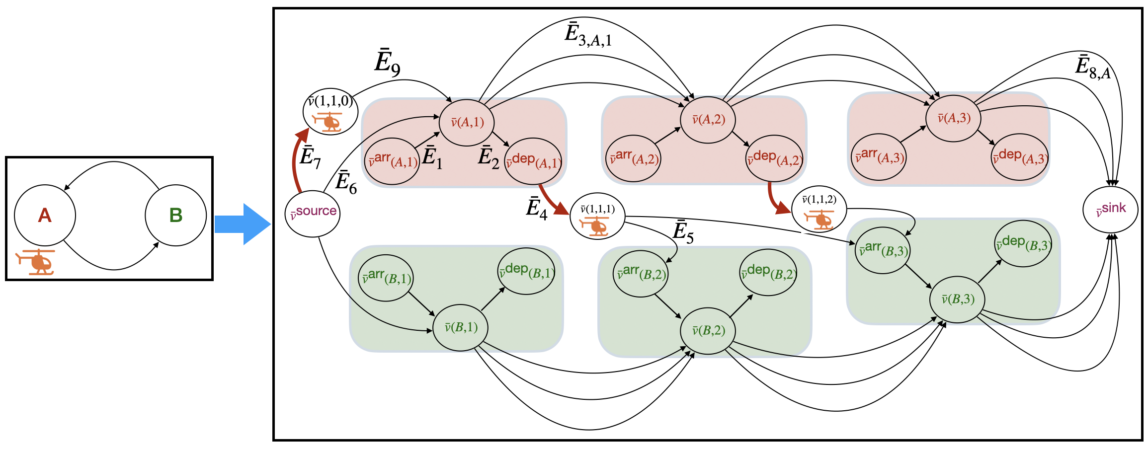
Figure 2: Auxiliary graph $\bar{G}$ constructed from an ATN with two vertiports and one aircraft over three time slots.

4 Optimization Algorithm

In this section, we formulate (6) as a mixed binary linear program (MBLP), as shown in (16). We derive this in three steps. First, in Section 4.1, we construct a time-extended flow network, where vertices are vertiport-time and aircraft-time pairs with edges capturing capacity constraints and route allocation. Then, using binary variables ($\delta_{i,j,\tau}$ as formally defined later in (12d) and (12e)) to ensure that each aircraft is allocated one route, we formulate a mixed integer linear program (MILP (12)) in Section 4.2. This MILP has fewer binary variables than (6) when the number of unique departure times for any aircraft is less than the size of its menu. Finally, in Section 4.3, we show that the total unimodularity of the constraint matrix ($\bar{I}_{\star}$ in (12b)) guarantees that all flows are integral for each binary variable assignment, so we can drop the integrality constraint (12f) and get the final MBLP formulation (16).

4.1 Auxiliary Graph

We construct an auxiliary graph $\bar{G}=(\bar{V},\bar{E})$ as detailed below. Figure 2 shows a pictorial depiction.

• Set of vertices $\bar{V}=\cup_{\ell=1}^{3}\bar{V}_{\ell}$. We define these sets below:

  • $\bar{V}_{1}:=\{(\bar{\nu}(r,t),\bar{\nu}^{\textsf{arr}}(r,t),\bar{\nu}^{\textsf{dep}}(r,t))|r\in R,t\in[H]\}$:

    We consider three replica for each vertiport $r\in R$ at time $t\in[H]$, denoted as $\bar{\nu}(r,t),\bar{\nu}^{\textsf{arr}}(r,t),$ and $\bar{\nu}^{\textsf{dep}}(r,t)$.

  • $\bar{V}_{2}:=\{\bar{\nu}({i,j,\tau})|i\in F,j\in A_{i},\tau\in T^{\textsf{dep}}_{i,j}\}$:

    For each $i\in F,j\in A_{i},$ we consider one vertex corresponding to all routes that have the same departure time. More formally, for every $i\in F,j\in A_{i},$ define $T^{\textsf{dep}}_{i,j}:=\cup_{k\in m_{i,j}}\left\{t^{\textsf{dep}}_{i,j,k}\right\},$ to be the set of unique departure times amongst all routes. We consider one vertex corresponding to each $i\in F,j\in A_{i},$ and $\tau\in T^{\textsf{dep}}_{i,j}$, denoted as $\bar{\nu}({i,j,\tau})$.

  • $\bar{V}_{3}:=\{\bar{\nu}^{\textsf{source}},\bar{\nu}^{\textsf{sink}}\}$:

    $\bar{\nu}^{\textsf{source}}$ and $\bar{\nu}^{\textsf{sink}}$ denote the source and sink in the flow network (to be described shortly).

• Set of edges $\bar{E}=\cup_{\ell=1}^{9}\bar{E}_{\ell}\subseteq\bar{V}\times\bar{V}\times\mathbb{Z}_{+}\times\mathbb{Z}_{+}\times\mathbb{R}$, where each edge is identified with a tuple $(r,r^{\prime},\overline{\textbf{c}},\underline{\textbf{c}},\bar{\textbf{w}})$ such that $(i)$ $r,r^{\prime}\in R$ are the upstream and downstream vertiport on an edge, respectively, $(ii)$ $\overline{\textbf{c}},\underline{\textbf{c}}\in\mathbb{Z}_{+}$ are the upper and lower bound on the capacity of the edge, respectively, and $(iii)$ $\bar{\textbf{w}}\in\mathbb{R}$ is the edge weight.

  • $\bar{E}_{1}:=\{(\bar{\nu}^{\textsf{arr}}(r,t),\bar{\nu}(r,t),\overline{\textbf{c}}=\textsf{arr}(r,t),\underline{\textbf{c}}=0,\bar{\textbf{w}}=0)|r\in R,t\in[H]\}$.

  • $\bar{E}_{2}:=\{(\bar{\nu}(r,t),\bar{\nu}^{\textsf{dep}}(r,t),\overline{\textbf{c}}=\textsf{dep}(r,t),\underline{\textbf{c}}=0,\bar{\textbf{w}}=0)|r\in R,t\in[H]\}$.

  • $\bar{E}_{3}:=\cup_{r\in R,t\in[H-1]}\bar{E}_{3,r,t}$:

    For every $r\in R,t\in[H-1]$, we consider $\textsf{park}(r,t)$ number of edges connecting $\bar{\nu}(r,t)$ and $\bar{\nu}(r,t+1)$. We denote this set by $\bar{E}_{3,r,t}$. For any $q\in[\textsf{park}(r,t)]$, we denote the $q-$th edge in $\bar{E}_{3,r,t}$ by $e_{q,r,t}$ which is defined to be the following tuple

    $$e_{q,r,t}=(\bar{\nu}(r,t),\bar{\nu}(r,t+1),\overline{\textbf{c}}=1,\underline{\textbf{c}}=0,\bar{\textbf{w}}=-\lambda(C_{r,t}(q)-C_{r,t}(q-1))).$$

  • $\bar{E}_{4}:=\{(\bar{\nu}^{\textsf{dep}}(r^{\textsf{orig}}_{i,j},\tau),\bar{\nu}({i,j,\tau}),\overline{\textbf{c}}=\underline{\textbf{c}}=\delta_{i,j,\tau},\bar{\textbf{w}}=0)|i\in F,j\in A_{i},\tau\in T_{i,j}^{\textsf{dep}}\backslash\{0\}\}$:

    $\delta_{i,j,\tau}\in\{0,1\}$ is a variable defined later.

  • $\bar{E}_{5}:=\{(\bar{\nu}({i,j,t^{\textsf{dep}}_{i,j,k}}),\bar{\nu}^{\textsf{arr}}({r^{\textsf{dest}}_{i,j,k}},t^{\textsf{arr}}_{i,j,k}),\overline{\textbf{c}}=1,\underline{\textbf{c}}=0,\bar{\textbf{w}}=\rho_{i}b_{i,j,k})|i\in F,j\in A_{i},k\in m_{i,j}\}$.

  • $\bar{E}_{6}:=\{(\bar{\nu}^{\textsf{source}},\bar{\nu}(r,1),\overline{\textbf{c}}=\underline{\textbf{c}}=\bar{S}(r)-\sum_{i\in F}\sum_{j\in A_{i}}\delta_{i,j,0}\mathbf{1}(r^{\textsf{orig}}_{i,j}=r),\bar{\textbf{w}}=0)|r\in R\}$.

  • $\bar{E}_{7}:=\{(\bar{\nu}^{\textsf{source}},\bar{\nu}(i,j,0),\overline{\textbf{c}}=\underline{\textbf{c}}=\delta_{i,j,0},\bar{\textbf{w}}=\rho_{i}b_{i,j,\varnothing})|i\in F,j\in A_{i}\}$:

    $\delta_{i,j,0}\in\{0,1\}$ is a variable which would be defined shortly, and $b_{i,j,\varnothing}$ is the bid placed by aircraft $a_{i,j}$ on staying parked at the same location.

  • $\bar{E}_{8}:=\cup_{r\in R}\bar{E}_{8,r}$:

    For every $r\in R$, we consider $\textsf{park}(r,H)$ number of edges connecting $\bar{\nu}(r,H)$ and $\bar{\nu}^{\textsf{sink}}$. We denote these edges by $\bar{E}_{8,r}$. For any $q\in[\textsf{park}(r,t)]$, we denote the $q-$th edge in $\bar{E}_{8,r}$ by $e_{q,r,H}$ which is defined to be the following tuple

    $$e_{q,r,H}=(\bar{\nu}(r,H),\bar{\nu}^{\textsf{sink}},\overline{\textbf{c}}=1,\underline{\textbf{c}}=0,\bar{\textbf{w}}=-\lambda(C_{r,H}(q)-C_{r,H}(q-1))).$$

  • $\bar{E}_{9}:=\{(\bar{\nu}(i,j),\bar{\nu}(r^{\textsf{orig}}_{i,j},1),\overline{\textbf{c}}=\underline{\textbf{c}}=\delta_{i,j,0},\bar{\textbf{w}}=0)|i\in F,j\in A_{i}\}$.

Remark 4.1.

In the preceding construction, the capacity of any outgoing edge (resp. incoming edge) from a node which does not have an incoming edge (resp. outgoing edge), other than $\bar{\nu}^{\textsf{source}}$ and $\bar{\nu}^{\textsf{sink}}$, is set to 0.

4.2 Mixed Integer Linear Program Formulation

For the construction of auxiliary graph presented in Section 4.1, we concatenate the weight, upper capacity bound, and lower capacity bound of each edge as $\overline{\mathbf{W}}\in\mathbb{R}^{|\bar{E}|}$, $\mathbf{\overline{C}}(\delta)\in\mathbb{Z}_{+}^{|\bar{E}|}$, and $\mathbf{\underline{C}}(\delta)\in\mathbb{Z}_{+}^{|\bar{E}|}$, respectively. Define an incidence matrix of the graph $\bar{G}$ as $\bar{I}\in\{-1,0,1\}^{|\bar{V}|\times|\bar{E}|}$, where

$$\bar{I}_{ij}=\begin{cases}1,&\text{if edge $j$ ends at vertex $i$,}\\ -1,&\text{if edge $j$ starts from vertex $i$,}\\ 0,&\text{otherwise}.\end{cases}$$ (11)

Defining a truncated incidence matrix $\bar{I}_{\star}$ obtained from $\bar{I}$ by removing rows corresponding to $\bar{\nu}^{\textsf{source}}$ and $\bar{\nu}^{\textsf{sink}}$, we consider the following optimization formulation (which will be shown to be crucial in computation of (6)).

$$\max_{\begin{subarray}{c}\mathbf{A},\delta\end{subarray}}~{}\overline{\mathbf{W}}^{\top}\mathbf{A}$$ (12a)

$$\ \text{s.t. }\ \ \bar{I}_{\star}\mathbf{A}=\mathbf{0}$$ (12b)

$$\ \ \ \ \ \ \ \mathbf{\underline{C}}(\delta)\leq\mathbf{A}\leq\mathbf{\overline{C}}(\delta)$$ (12c)

$$\ \ \ \ \ \ \ \sum_{\tau\in T_{i,j}^{\textsf{dep}}}\delta_{i,j,\tau}=1,\forall~{}i\in F,j\in A_{i}$$ (12d)

$$\ \ \ \ \ \ \ \delta_{i,j,\tau}\in\{0,1\},\forall~{}i\in F,j\in A_{i},\tau\in T_{i,j}^{\textsf{dep}}$$ (12e)

$$\ \ \ \ \ \ \ \mathbf{A}\in\mathbb{Z}^{|\bar{E}|}_{+}$$ (12f)

$$\ \ \ \ \ \ \ {\mathbf{A}_{e_{q+1,r,t}}\!\leq\!\mathbf{A}_{e_{q,r,t}},\forall r\in R,t\in[H],q\in[\textsf{park}(r,t)-1]}.$$ (12g)

Here, (12b) denotes the “flow balance” constraint at every node in $\bar{V}\backslash\bar{V}_{3}$; (12c) denotes the capacity constraints where we have explicitly denoted the dependence of constraints on $\delta$ (cf. definitions of $\bar{E}_{4}$ and $\bar{E}_{7}$); (12d) and (12e) denote the constraint that each aircraft must be allocated exactly one route; (12f) denotes the integrality constriants; (12g) denotes additional constraints which require that edges in $\bar{E}_{3,r,t}$ and $\bar{E}_{8,r}$ are allocated in an increasing order.

Next, we highlight the connection between the optimization problems (6) and (12).

Proposition 4.2.

Suppose $(A^{\dagger},\delta^{\dagger})$ is an optimal solution to (12). Then $\overline{\textbf{W}}^{\top}\textbf{A}^{\dagger}=\max_{x\in X}\textsf{SW}(x;B)$. Additionally, using $A^{\dagger}$ we can uniquely determine $x^{\dagger}\in X$ such that $x^{\dagger}\in\underset{x\in X}{\arg\max}~{}\textsf{SW}(x;B)$.

Proof.

First, we show that, for every $x\in X$, there exists a unique $(\textbf{A}(x),\delta(x))$ satisfying (12b)-(12g) and $\overline{\textbf{W}}^{\top}\textbf{A}(x)=\textsf{SW}(x;B).$ Indeed, we construct $(\textbf{A}(x),\delta(x))$ such that

• for every $e\!\in\!\bar{E}_{5}$, where $(\bar{\nu}({i,j,t^{\textsf{dep}}_{i,j,k}}),\bar{\nu}^{\textsf{arr}}({r^{\textsf{dest}}_{i,j,k},t^{\textsf{arr}}_{i,j,k}}))\in e$ for some $i\in F,j\in A_{i},k\in m_{i,j}$, it holds that $\textbf{A}_{e}(x)=x_{i,j,k}$;

• for every $r\in R,t\in[H]$, and $q\in[\textsf{park}(r,t)]$, it holds that $\textbf{A}_{e}(x)=\mathbf{1}(q\leq S(r,t,x))$, where $e$ is the $q-$th edge in $\bar{E}_{3,r,t}\cup\bar{E}_{8,r}.$

The above construction specifies the values of $\textbf{A}_{e}(x)$ for $e\in\bar{E}_{3}\cup\bar{E}_{5}\cup\bar{E}_{8}$. Additionally, by Lemma 4.3, there exists a unique feasible solution $(\textbf{A}(x),\delta(x))$ that satisfied (12b)-(12g) , and we get

$$\overline{\mathbf{W}}^{\top}\mathbf{A}(x)=\sum_{e\in\bar{E}}\bar{\textbf{w}}_{e}\mathbf{A}_{e}(x)=\sum_{e\in\bar{E}_{3}\cup\bar{E}_{5}\cup\bar{E}_{7}\cup\bar{E}_{8}}\bar{\textbf{w}}_{e}\mathbf{A}_{e}(x),$$

where the last equality holds because $\bar{\textbf{w}}_{e}=0$ for $e\in\bar{E}_{1}\cup\bar{E}_{2}\cup\bar{E}_{4}\cup\bar{E}_{6}\cup\bar{E}_{9}.$

Then, we examine each term. First, observe the following.

$$\sum_{e\in\bar{E}_{5}}\bar{\textbf{w}}_{e}\mathbf{A}_{e}(x) =\sum_{i\in F}\sum_{j\in A_{i}}\sum_{k\in m_{i,j}}\rho_{i}b_{i,j,k}x_{i,j,k}.$$

$$\sum_{e\in\bar{E}_{7}}\bar{\textbf{w}}_{e}\mathbf{A}_{e}(x) =\sum_{i\in F}\sum_{j\in A_{i}}\rho_{i}b_{i,j,\phi}x_{i,j,0}.$$

Next, we use the definition of weights in $\bar{E}_{3,r,t}$.

$$\sum_{e\in\bar{E}_{3}}\bar{\textbf{w}}_{e}\mathbf{A}_{e}(x)=\sum_{r\in R}\sum_{t=1}^{H-1}\sum_{e\in\bar{E}_{3,r,t}}\bar{\textbf{w}}_{e}\mathbf{A}_{e}(x)$$

$$=\sum_{r\in R}\sum_{t=1}^{H-1}\sum_{q=1}^{\textsf{park}(r,t)}\bar{\textbf{w}}_{e_{q,r,t}}\mathbf{A}_{e_{q,r,t}}(x)$$

$$=-\lambda\sum_{r\in R}\sum_{t=1}^{H-1}\sum_{q=1}^{S(r,t,x)}\left(C_{r}(q)-C_{r}(q-1)\right)$$

$$=-\lambda\sum_{r\in R}\sum_{t=1}^{H-1}C_{r}(S(r,t,x)).$$

Similarly, we get $\sum_{e\in\bar{E}_{8}}\bar{\textbf{w}}_{e}\mathbf{A}_{e}(x)=-\lambda\sum_{r\in R}C_{r}(S(r,H,x))$. To summarize, we obtain

$$\overline{\textbf{W}}^{\top}\textbf{A}(x)=\textsf{SW}(x;B).$$ (13)

Using this, we conclude that

$$\max_{x\in X}\textsf{SW}(x;B)=\max_{x\in X}\overline{\textbf{W}}^{\top}\textbf{A}(x)$$ (14)

$$\leq\max_{(\textbf{A},\delta)~{}\text{s.t.}~{}\eqref{eq: ILP_FlowBalance}-\eqref{eq: ILP_Increasingq_t}}\overline{\textbf{W}}^{\top}\textbf{A}=\overline{\textbf{W}}^{\top}\textbf{A}^{\dagger}.$$

Next, we show that for every $(\textbf{A},\delta)$ satisfying (12b)-(12g), there exists $x(\textbf{A},\delta)\in X$ such that $\textsf{SW}(x(\textbf{A},\delta))=\overline{\textbf{W}}^{\top}\textbf{A}$. Indeed, we construct $x(\textbf{A},\delta)$ such that for every $i\in F,j\in A_{i},k\in m_{i,j}$ it holds that $x_{i,j,k}=\textbf{A}_{e}$ for $e\in\bar{E}_{5}$ such that $(\bar{\nu}({i,j,t^{\textsf{dep}}_{i,j,k}}),\bar{\nu}^{\textsf{arr}}({r^{\textsf{dest}}_{i,j,k}},t^{\textsf{arr}}_{i,j,k}))\in e$ or $e\in\bar{E}_{9}$ such that $(\bar{\nu}({i,j,0}),\bar{\nu}({r^{\textsf{dest}}_{i,j,k}},1))\in e$. Note that due to capacity constraints on these edges, $x_{i,j,k}\in\{0,1\}$. Additionally, the flow balance at the nodes of the form $\bar{\nu}(i,j,\tau)$, for some $i\in F,j\in A_{i},\tau\in T_{i,j}^{\textsf{dep}}$, ensures that

$$\delta_{i,j,\tau}=\sum\limits_{k\in m_{i,j}}\sum\limits_{e\in\bar{E}_{9}}\textbf{A}_{e}\mathbf{1}((\bar{\nu}({i,j,0}),\bar{\nu}({r^{\textsf{dest}}_{i,j,k},1}))\in e,\tau=0)$$

$$+\sum\limits_{k\in m_{i,j}}\sum\limits_{e\in\bar{E}_{5}}\textbf{A}_{e}\mathbf{1}((\bar{\nu}({i,j,t^{\textsf{dep}}_{i,j,k}}),\bar{\nu}^{\textsf{arr}}({r^{\textsf{dest}}_{i,j,k},t^{\textsf{arr}}_{i,j,k}}))\in e,\tau=t^{\textsf{dep}}_{i,j,k}).$$

Summing over $\tau$, we get

$$\sum_{\tau\in T_{i,j}^{\textsf{dep}}}\!\!\delta_{i,j,\tau}=\!\!\sum_{k\in m_{i,j}}\sum_{e\in\bar{E}_{9}}\textbf{A}_{e}\mathbf{1}((\bar{\nu}({i,j,0}),\bar{\nu}({r^{\textsf{dest}}_{i,j,k},1}))\in e)$$

$$\quad+\sum_{k\in m_{i,j}}\sum_{e\in\bar{E}_{5}}\textbf{A}_{e}\mathbf{1}((\bar{\nu}({i,j,t^{\textsf{dep}}_{i,j,k}}),\bar{\nu}^{\textsf{arr}}({r^{\textsf{dest}}_{i,j,k},t^{\textsf{arr}}_{i,j,k}}))\in e)$$

$$\quad\quad\quad\quad\ =\sum_{k\in m_{i,j}}x_{i,j,k}(\textbf{A},\delta).$$

Using (12d), we conclude that $\sum_{k\in m_{i,j}}x_{i,j,k}(\textbf{A},\delta)=1$.

Next, we use the flow balance at nodes of the form $\bar{\nu}^{\textsf{arr}}(r,t)$, for every $r\in R,t\in[H]$, to ensure that

$$\sum\limits_{\begin{subarray}{c}i\in F,j\in A_{i},\\ k\in m_{i,j},e\in\bar{E}_{5}\end{subarray}}\textbf{A}_{e}\mathbf{1}((\bar{\nu}({i,j,t^{\textsf{dep}}_{i,j,k}}),\bar{\nu}^{\textsf{arr}}({r^{\textsf{dest}}_{i,j,k},t^{\textsf{arr}}_{i,j,k}}))\in e,r^{\textsf{dest}}_{i,j,k}=r,t^{\textsf{arr}}_{i,j,k}=t)\leq\textsf{arr}(r,t).$$

By $\sum_{e\in\bar{E}_{5}}\textbf{A}_{e}\mathbf{1}((\bar{\nu}({i,j,t^{\textsf{dep}}_{i,j,k}}),\bar{\nu}^{\textsf{arr}}({r^{\textsf{dest}}_{i,j,k},t^{\textsf{arr}}_{i,j,k}}))\in e)=x_{i,j,k}(\textbf{A},\delta)$, we get

$$\sum_{i\in F}\sum_{j\in A_{i}}\sum_{k\in m_{i,j}}{x}_{i,j,k}\mathbf{1}(r^{\textsf{dest}}_{i,j,k}=r,t^{\textsf{arr}}_{i,j,k}=t)\leq\textsf{arr}(r,t)$$

Note that if $t=1$, the arrival capacity constraints are trivially satisfied since there is no incoming aircraft. Analogously, the flow balance equations at the nodes of the form $\bar{\nu}^{\textsf{dep}}(r,t)$, for some $r\in R,t\in[H]$, ensure that $\sum_{i\in F}\sum_{j\in A_{i}}\sum_{k\in m_{i,j}}{x}_{i,j,k}\mathbf{1}(r^{\textsf{orig}}_{i,j}=r,t^{\textsf{dep}}_{i,j,k}=t)\leq\textsf{dep}(r,t).$ Finally, we can establish $S(r,t,x(\textbf{A},\delta))=\sum_{q=1}^{\textsf{park}(r,t)}\textbf{A}_{e_{q,r,t}}$ through the flow balance equation at $\bar{\nu}(r,t)$ and (1). Since $\sum_{q=1}^{\textsf{park}(r,t)}\textbf{A}_{e_{q,r,t}}\leq\textsf{park}(r,t)$, due to the capacity constraints on the edge $\bar{E}_{3,r,t}$, it holds that $S(r,t,x(\textbf{A},\delta))\leq\textsf{park}(r,t)$. Thus, we conclude that $x(\textbf{A},\delta)\in X$.

Additionally, using the analysis to show (13) in the backward direction and the construction of $x(\textbf{A},\delta)$, we can establish that $\textsf{SW}(x(\textbf{A},\delta))=\overline{W}^{\top}\textbf{A}$. Thus, we conclude that

$$\overline{\textbf{W}}^{\top}\textbf{A}^{\dagger}=\max_{(\textbf{A},\delta)~{}\text{s.t.}~{}\eqref{eq: ILP_FlowBalance}-\eqref{eq: ILP_Increasingq_t}}\overline{\textbf{W}}^{\top}\textbf{A}$$ (15)

$$=\max_{(\textbf{A},\delta)~{}\text{s.t.}~{}\eqref{eq: ILP_FlowBalance}-\eqref{eq: ILP_Increasingq_t}}\textsf{SW}(x(\textbf{A},\delta))\leq\max_{x\in X}\textsf{SW}(x).$$

By (14) and (LABEL:eq:_reverse), we get $\overline{\textbf{W}}^{\top}\textbf{A}^{\dagger}=\max_{x\in X}\textsf{SW}(x)$. ∎

Next, we present a technical lemma used in the proof of Proposition 4.2.

Lemma 4.3.

Given the values of $\textbf{A}_{e}$ for $e\in\bar{E}_{3}\cup\bar{E}_{5}\cup\bar{E}_{8}$ that satisfy the capacity constraints (12c), there exists a unique feasible solution $(\textbf{A},\delta)$ that satisfies (12b)-(12g).

Proof.

First, note that any feasible solution to (12b)-(12g) has the same value of $\textbf{A}_{e}(x)$ for $e\in\bar{E}_{6}\cup\bar{E}_{7}\cup\bar{E}_{9}$ since the lower and upper bound on capacity are the same on these edges by construction. Thus, it is sufficient to show that the values of $\textbf{A}_{e}$ for $e\in\bar{E}_{3}\cup\bar{E}_{5}\cup\bar{E}_{6}\cup\bar{E}_{7}\cup\bar{E}_{8}\cup\bar{E}_{9}$, uniquely determine a feasible solution $(\textbf{A},\delta)$ that satisfies (12b)-(12g). Particularly, we will show that we can uniquely recover the values of $\textbf{A}_{e}$ for $e\in\bar{E}_{1}\cup\bar{E}_{2}\cup\bar{E}_{4}.$

To show this claim, we leverage the flow balance constraint (12b) at every node. Below, we state the incoming and outgoing edges from every type of node in the network.

Vertex	Incoming Edges	Outgoing Edges
$\bar{\nu}^{\textsf{arr}}(r,t)$	${\bar{E}_{5}}$	$\bar{E}_{1}$
$\bar{\nu}(i,j,\tau)$	$\bar{E}_{4}$	${\bar{E}_{5}}$
$\bar{\nu}^{\textsf{dep}}(r,t)$	$\bar{E}_{2}$	${\bar{E}_{4}}$
$\bar{\nu}(i,j,0)$	$\bar{E}_{7}$	$\bar{E}_{9}$
$\bar{\nu}(r,t)$	$\bar{E}_{1},\bar{E}_{3},\bar{E}_{6},\bar{E}_{9}$	$\bar{E}_{2},\bar{E}_{3},\bar{E}_{8}$

Note that flow balance at nodes of the form $\bar{\nu}^{\textsf{arr}}(r,t)$ will determine the values $\textbf{A}_{e}$ on edge $\bar{E}_{1}$, as we know these values for all edges in the set $\bar{E}_{5}$. Next, flow balance at nodes of the form $\bar{\nu}(i,j,\tau)$ will determine the values $\textbf{A}_{e}$ on edge $\bar{E}_{4}$, as we know these values for edges $\bar{E}_{5}$. This and the capacity constraints on $\bar{E}_{4}$, ensure that we know the value of $\delta$. Next, flow balance at nodes of the form $\bar{\nu}^{\textsf{dep}}(r,t)$ will determine the values $\textbf{A}_{e}$ on edge $\bar{E}_{2}$, as we can uniquely determine these values on $\bar{E}_{4}$. Finally, flow balance at nodes of the form $\bar{\nu}(r,t)$ will determine the values $\textbf{A}_{e}$ on edge $\bar{E}_{2}$, as we can uniquely determine these values on $\bar{E}_{1}\cup\bar{E}_{3}\cup\bar{E}_{6}\cup\bar{E}_{8}\cup\bar{E}_{9}$.

∎

4.3 Reduction to Mixed Binary Linear Program

Instead of solving (12), we can obtain $(\textbf{A}^{\dagger},\delta^{\dagger})$ by solving the following MBLP. We establish this fact in Proposition 4.4.

$$\max_{\begin{subarray}{c}\mathbf{A},\delta\end{subarray}}~{}\overline{\mathbf{W}}^{\top}\mathbf{A}$$ (16a)

$$\ \text{s.t. }\eqref{eq: ILP_FlowBalance}-\eqref{eq: ILP_VariableDelta}$$ (16b)

$$\ \ \ \ \ \ \ \mathbf{A}\in\mathbb{R}^{|\bar{E}|}_{+}.$$ (16c)

Proposition 4.4.

The optimal values of (12) and (16) are equal.

Proof.

First, we prove that we can drop (12g) when solving (12). Suppose there exists $r\in R,t\in[H]$, $q\in[\textsf{park}(r,t)-1]$ such that $\textbf{A}^{\dagger}_{q,r,t}<\textbf{A}^{\dagger}_{q+1,r,t}$. By swapping the value of $\textbf{A}^{\dagger}_{q+1,r,t}$ with that of $\textbf{A}^{\dagger}_{q,r,t}$, we get a new feasible allocation with a weakly higher objective value. This is because $\bar{\textbf{w}}_{q+1,r,t}\leq\bar{\textbf{w}}_{q,r,t}$ as $\lambda\geq 0$ and $C_{r,t}(\cdot)$ is discrete convex.

Additionally, we can also relax (12f) to (16c) because, for any feasible value of $\delta$, the optimization problem (12) is an integer linear program where the constraint matrix $\bar{I}_{\star}$ satisfies total unimodularity, so it is guaranteed to have an integral solution (Schrijver, 1998, Chapter 19). ∎

For any fixed values of binary variables $(\delta_{i,j,\tau})_{i\in F,j\in A_{i},\tau\in T_{i,j}^{\textsf{dep}}}$, the optimization problem (12) is in fact a maximum-weight flow problem. Thus, one can enumerate all the departure time combinations, and solve each maximum-weight flow problem with the number of scenarios being $\prod_{i\in F,j\in A_{i}}|\{t^{\textsf{dep}}_{i,j,k}|k\in m_{i,j}\}|$. The complete problem can be solved efficiency using the above MBLP approach, which will provide speed-up due to some techniques implemented in commercial solvers such as branch and bound, cutting-plane methods, etc.

5 Discussions

We show how the proposed mechanism generalizes existing works in Section 5.1 and present some extensions in Section 5.2.

5.1 Connections to Existing Mechanisms

Consider $H=1$, $\textsf{arr}(r,1)=\infty$, $\textsf{dep}(r,1)=\infty$, $\forall r\in R$, and $|A_{i}|=1$, $\forall i\in F$.

• Air Traffic Protocol: When we treat each vertiport $r\in R$ as a sector with $\textsf{park}(r,1)$ being the sector capacity, our model generalizes the problem studied in (Qin and Balakrishnan, 2022), where the authors did not consider arrival and departure capacities and assumed fleet operators with single aircraft.

• Airport Time Slot Auction: When we treat each vertiport $r\in R$ as a time slot with $\textsf{park}(r,1)$ being the slot capacity, our model subsumes the framework in (Dixit et al., 2023). Therefore, our formulation becomes a two-sided matching problem as detailed in (Dixit et al., 2023) and is subject to a faster strongly polynomial-time algorithm.

5.2 Extensions of the Proposed Mechanism

Our framework can be easily extended to incorporate the following aspects.

• External Demand: Aircraft that are not available in the service area of the SP at $t=0$ can be incorporated in our framework by setting $r^{\textsf{orig}}_{i,j}=\mathcal{O}$ and $t^{\textsf{dep}}_{i,j,k}=0,\forall k\in m_{i,j}$, where $\mathcal{O}$ denotes an auxiliary vertiport denoting aircraft coming from outside of the service area of SP.

• Entire Trajectory: We can extend each route to an entire trajectory with multiple vertiport-time pairs. By setting a binary variable for each route and combining those variables when two routes only differ in one time slot, we can apply the same MBLP approach.

• Cancellation Policy: It is possible to cancel or re-allocate some of the previously scheduled flights due to changing vertiport capacities or newly emerging aircraft. While there is no single criterion for re-allocation, it is typical to consider three aspects: congestion, efficiency, and fairness, where we cancel flights from congested vertiports, with low valuations, or at random, respectively.

6 Conclusion

In this work, we propose an auction mechanism to incentivize fleet operators to report their valuations truthfully and consequently perform a socially optimal vertiport reservation. This approach adapts the popular Vickrey–Clarke–Groves mechanism while considering the egalitarian, congestion-aware, and computational issues. The proposed framework could be of interest beyond air traffic management, such as multi-robot coordination. In a follow-up paper, we shall provide a numerical analysis of the mechanism’s performance. Several interesting avenues exist for future research. First, we would like to extend the auction mechanism to include waypoints in airspace, thus moving toward a more complete air traffic flow management formulation. Second, different fairness notions have been considered in airspace and other areas, such as reversals, takeovers, and priority guarantees (Bertsimas and Gupta, 2016; Su et al., 2023). It is interesting to compare different formulations, both theoretically and empirically.

Appendix A Table of Notations

Notation	Description
$R$	Set of vertiports
$F$	Set of fleet operators
$A_{i}$	Set of eVTOL aircraft in the fleet of operator $i\in F$
$H$	Scheduling horizon
$a_{i,j}$	The identification of the $j-$th aircraft in $A_{i}$
$r^{\textsf{orig}}_{i,j}$	Origin vertiport of aircraft $a_{i,j}$
$m_{i,j}$	Set of available routes of aircraft $a_{i,j}$
$t^{\textsf{dep}}_{i,j,k}$	Departure time for aircraft $a_{i,j}$ if it chooses the $k-$th route in $m_{i,j}$
$r^{\textsf{dest}}_{i,j,k}$	Destination vertiport of aircraft $a_{i,j}$ if it chooses the $k-$th route in $m_{i,j}$
$t^{\textsf{arr}}_{i,j,k}$	Arrival time of aircraft $a_{i,j}$ at $r^{\textsf{dest}}_{i,j,k}$ if it chooses the $k-$th route in $m_{i,j}$
$v_{i,j,k}$	Valuation derived by aircraft $a_{i,j}$ if it is allocated the $k-$th route in $m_{i,j}$
$b_{i,j,k}$	Bid for aircraft $a_{i,j}$ to be allocated the the $k-$th route in $m_{i,j}$
${x}_{i,j,k}$	Binary variable denoting whether aircraft $a_{i,j}$ is allocated the $k-$th route in $m_{i,j}$
$S(r,t,x)$	Number of aircraft at vertiport $r\in R$ at time $t\in[H]$ under allocation $x$
$\textsf{arr}(r,t)$	Arrival capacity of vertiport $r\in R$ at time $t\in[H]$
$\textsf{dep}(r,t)$	Departure capacity of vertiport $r\in R$ at time $t\in[H]$
$\textsf{park}(r,t)$	Parking capacity of vertiport $r\in R$ at time $t\in[H]$
$\textsf{SW}(x;V)$	Social welfare under allocation $x$ if the valuation of aircraft is $V=(v_{i,j,k})_{i\in F,j\in A_{i},k\in m_{i,j}}$
$\theta$	Pseudo-bids
$C_{r,t}(\cdot)$	Congestion function of vertiport $r\in R$ at time $t\in[H]$
$\bar{G}$	Auxiliary graph for the optimization algorithm
$\bar{V}$	Set of vertices of the auxiliary graph
$\bar{E}$	Set of edges of the auxiliary graph

References

- Administration (2023) Federal Aviation Administration. Urban air mobility concept of operations 2.0. Technical report, Federal Aviation Administration, 2023. URL https://www.faa.gov/air-taxis/uam_blueprint.
- Ball et al. (2018) Michael O. Ball, Frank Berardino, and Mark Hansen. The use of auctions for allocating airport access rights. Transportation Research Part A: Policy and Practice, 114:186–202, 2018. ISSN 0965-8564. doi: https://doi.org/10.1016/j.tra.2017.09.026. URL https://www.sciencedirect.com/science/article/pii/S0965856416303287.
- Ball et al. (2020) Michael O. Ball, Alexander S. Estes, Mark Hansen, and Yulin Liu. Quantity-contingent auctions and allocation of airport slots. Transportation Science, 54(4):858–881, 2020. doi: 10.1287/trsc.2020.0995. URL https://doi.org/10.1287/trsc.2020.0995.
- Basso and Zhang (2010) Leonardo J. Basso and Anming Zhang. Pricing vs. slot policies when airport profits matter. Transportation Research Part B: Methodological, 44(3):381–391, 2010. ISSN 0191-2615. doi: https://doi.org/10.1016/j.trb.2009.09.005. URL https://www.sciencedirect.com/science/article/pii/S0191261509001179. Economic Analysis of Airport Congestion.
- (5) Josh Bertram and Peng Wei. An Efficient Algorithm for Self-Organized Terminal Arrival in Urban Air Mobility. doi: 10.2514/6.2020-0660. URL https://arc.aiaa.org/doi/abs/10.2514/6.2020-0660.
- Bertsimas and Gupta (2016) Dimitris Bertsimas and Shubham Gupta. Fairness and collaboration in network air traffic flow management: An optimization approach. Transportation Science, 50(1):57–76, 2016. doi: 10.1287/trsc.2014.0567. URL https://doi.org/10.1287/trsc.2014.0567.
- Bertsimas and Patterson (1998) Dimitris Bertsimas and Sarah Stock Patterson. The air traffic flow management problem with enroute capacities. Operations Research, 46(3):406–422, 1998. doi: 10.1287/opre.46.3.406. URL https://doi.org/10.1287/opre.46.3.406.
- Bertsimas and Patterson (2000) Dimitris Bertsimas and Sarah Stock Patterson. The traffic flow management rerouting problem in air traffic control: A dynamic network flow approach. Transportation Science, 34(3):239–255, 2000. doi: 10.1287/trsc.34.3.239.12300. URL https://doi.org/10.1287/trsc.34.3.239.12300.
- Bertsimas et al. (2011) Dimitris Bertsimas, Guglielmo Lulli, and Amedeo Odoni. An integer optimization approach to large-scale air traffic flow management. Operations Research, 59(1):211–227, 2011. doi: 10.1287/opre.1100.0899. URL https://doi.org/10.1287/opre.1100.0899.
- Bichler et al. (2023) Martin Bichler, Peter Gritzmann, Paul Karaenke, and Michael Ritter. On airport time slot auctions: A market design complying with the iata scheduling guidelines. Transportation Science, 57(1):27–51, 2023.
- Carlin and Park (1970) Alan Carlin and R. E. Park. Marginal cost pricing of airport runway capacity. The American Economic Review, 60(3):310–319, 1970. ISSN 00028282. URL http://www.jstor.org/stable/1817981.
- Chin et al. (2021) Christopher Chin, Karthik Gopalakrishnan, Maxim Egorov, Antony Evans, and Hamsa Balakrishnan. Efficiency and fairness in unmanned air traffic flow management. IEEE Transactions on Intelligent Transportation Systems, 22(9):5939–5951, 2021. doi: 10.1109/TITS.2020.3048356.
- Chin et al. (2023a) Christopher Chin, Karthik Gopalakrishnan, Hamsa Balakrishnan, Maxim Egorov, and Antony Evans. Protocol-based congestion management for advanced air mobility. Journal of Air Transportation, 31(1):35–44, 2023a.
- Chin et al. (2023b) Christopher Chin, Victor Qin, Karthik Gopalakrishnan, and Hamsa Balakrishnan. Traffic management protocols for advanced air mobility. Frontiers in Aerospace Engineering, 2:1176969, 2023b.
- Cohen et al. (2021) Adam P Cohen, Susan A Shaheen, and Emily M Farrar. Urban air mobility: History, ecosystem, market potential, and challenges. IEEE Transactions on Intelligent Transportation Systems, 22(9):6074–6087, 2021.
- Dixit et al. (2023) Aasheesh Kumar Dixit, Garima Shakya, Suresh Kumar Jakhar, and Swaprava Nath. Algorithmic mechanism design for egalitarian and congestion-aware airport slot allocation. Transportation Research Part E: Logistics and Transportation Review, 169:102971, 2023. ISSN 1366-5545. doi: https://doi.org/10.1016/j.tre.2022.102971. URL https://www.sciencedirect.com/science/article/pii/S1366554522003489.
- (17) Antony D. Evans, Maxim Egorov, and Steven Munn. Fairness in Decentralized Strategic Deconfliction in UTM. doi: 10.2514/6.2020-2203. URL https://arc.aiaa.org/doi/abs/10.2514/6.2020-2203.
- (18) Nelson M. Guerreiro, George E. Hagen, Jeffrey M. Maddalon, and Ricky W. Butler. Capacity and Throughput of Urban Air Mobility Vertiports with a First-Come, First-Served Vertiport Scheduling Algorithm. doi: 10.2514/6.2020-2903. URL https://arc.aiaa.org/doi/abs/10.2514/6.2020-2903.
- Kleinbekman et al. (2018) Imke C. Kleinbekman, Mihaela A. Mitici, and Peng Wei. evtol arrival sequencing and scheduling for on-demand urban air mobility. In 2018 IEEE/AIAA 37th Digital Avionics Systems Conference (DASC), pages 1–7, 2018. doi: 10.1109/DASC.2018.8569645.
- Mehta and Vazirani (2020) Ruta Mehta and Vijay V. Vazirani. An incentive compatible, efficient market for air traffic flow management. Theoretical Computer Science, 818:41–50, 2020. ISSN 0304-3975. doi: https://doi.org/10.1016/j.tcs.2018.09.006. URL https://www.sciencedirect.com/science/article/pii/S0304397518305711. Computing and Combinatorics.
- Murota (2015) Kazuo Murota. Discrete convex analysis. Hausdorff Institute of Mathematics, Summer School (September 21–25, 2015), 2015.
- Myerson (1981) Roger B. Myerson. Optimal auction design. Mathematics of Operations Research, 6(1):58–73, 1981. doi: 10.1287/moor.6.1.58. URL https://doi.org/10.1287/moor.6.1.58.
- Nisan et al. (2007) N. Nisan, T. Roughgarden, E. Tardos, and V. V. Vazirani. Algorithmic Game Theory. Cambridge University Press, 2007.
- Odoni (1987) Amedeo R. Odoni. The flow management problem in air traffic control. In Amedeo R. Odoni, Lucio Bianco, and Giorgio Szegö, editors, Flow Control of Congested Networks, pages 269–288, Berlin, Heidelberg, 1987. Springer Berlin Heidelberg. ISBN 978-3-642-86726-2.
- Pertuiset and Santos (2014) Thomas Pertuiset and Georgina Santos. Primary auction of slots at european airports. Research in Transportation Economics, 45:66–71, 2014. ISSN 0739-8859. doi: https://doi.org/10.1016/j.retrec.2014.07.009. URL https://www.sciencedirect.com/science/article/pii/S0739885914000304. Pricing and Regulation in the Airline Industry.
- Qin and Balakrishnan (2022) Victor Qin and Hamsa Balakrishnan. Cost-aware congestion management protocols for advanced air mobility. 2022.
- Rassenti et al. (1982) S. J. Rassenti, V. L. Smith, and R. L. Bulfin. A combinatorial auction mechanism for airport time slot allocation. The Bell Journal of Economics, 13(2):402–417, 1982. ISSN 0361915X. URL http://www.jstor.org/stable/3003463.
- Roy and Tomlin (2007) Kaushik Roy and Claire J. Tomlin. Solving the aircraft routing problem using network flow algorithms. In 2007 American Control Conference, pages 3330–3335, 2007. doi: 10.1109/ACC.2007.4282854.
- Schrijver (1998) Alexander Schrijver. Theory of Linear and Integer Programming. John Wiley & Sons, Inc., USA, 1998. ISBN 0471908541.
- Seuken et al. (2022) Sven Seuken, Paul Friedrich, and Ludwig Dierks. Market design for drone traffic management. In Proceedings of the AAAI Conference on Artificial Intelligence, volume 36, pages 12294–12300, 2022.
- Shao et al. (2021) Quan Shao, Mengxue Shao, and Yang Lu. Terminal area control rules and evtol adaptive scheduling model for multi-vertiport system in urban air mobility. Transportation Research Part C: Emerging Technologies, 132:103385, 2021. ISSN 0968-090X. doi: https://doi.org/10.1016/j.trc.2021.103385. URL https://www.sciencedirect.com/science/article/pii/S0968090X21003843.
- Skorup (2019) Brent Skorup. Auctioning airspace. NCJL & Tech., 21:79, 2019.
- Su et al. (2023) Pan-Yang Su, Kuang-Hsun Lin, Yi-Yun Li, and Hung-Yu Wei. Priority-aware resource allocation for 5g mmwave multicast broadcast services. IEEE Transactions on Broadcasting, 69(1):246–263, 2023. doi: 10.1109/TBC.2022.3221696.
- Sun et al. (2023) Luying Sun, Peng Wei, and Weijun Xie. Fair and risk-averse urban air mobility resource allocation under uncertainties. Available at SSRN 4343979, 2023.
- Wang et al. (2023) Ben Wang, Zilong Deng, Xuan Ni, Kevin B Smith, Max Z Li, and Romesh Saigal. Learning-driven airspace congestion pricing for advanced air mobility. In AIAA SCITECH 2023 Forum, page 0547, 2023.
- Wei et al. (2023) Peng Wei, Paul Krois, Joseph Block, Paul Cobb, Gano Chatterji, and Cherie Kurian. Arrival management for high-density vertiport and terminal airspace operations. 2023.
- Wu et al. (2022) Pengcheng Wu, Xuxi Yang, Peng Wei, and Jun Chen. Safety assured online guidance with airborne separation for urban air mobility operations in uncertain environments. IEEE Transactions on Intelligent Transportation Systems, 23(10):19413–19427, 2022. doi: 10.1109/TITS.2022.3163657.