A Real-Time Rescheduling Algorithm for Multi-robot Plan Execution
Abstract
One area of research in multi-agent path finding is to determine how replanning can be efficiently achieved in the case of agents being delayed during execution. One option is to reschedule the passing order of agents, i.e., the sequence in which agents visit the same location. In response, we propose Switchable-Edge Search (SES), an A*-style algorithm designed to find optimal passing orders. We prove the optimality of SES and evaluate its efficiency via simulations. The best variant of SES takes less than 1 second for small- and medium-sized problems and runs up to 4 times faster than baselines for large-sized problems.
Introduction
Multi-Agent Path Finding (MAPF) is the problem of finding collision-free paths that move a team of agents from their start to goal locations. MAPF is fundamental to numerous applications, such as automated warehouses (Wurman, D’Andrea, and Mountz 2007; Kou et al. 2020), computer games (Silver 2005), and drone swarms (Hönig et al. 2018).
Classic MAPF models assume flawless execution. However, in real-world scenarios, agents may encounter unexpected delays due to mechanical differences, unforeseen events, localization errors, and so on. To accommodate such delays, existing research suggests the use of a Temporal Plan Graph (TPG) (Hönig et al. 2016). The TPG captures the precedence relationships within a MAPF solution and maintains them during execution. Each precedence relationship specifies an order for two agents to visit the same location. An agent advances to the next location in its path only if the corresponding precedence conditions are met. Consequently, if an agent experiences a delay, all other agents whose actions depend on this agent will pause. Despite its advantages of providing rigorous guarantees on collision-freeness and deadlock-freeness, the use of TPG can introduce a significant number of waits into the execution results due to the knock-on effect in the precedence relationship.
In this paper, we adopt a variant of TPG, named Switchable TPG (STPG) (Berndt et al. 2020). STPG allows for the modification of some precedence relationships in a TPG, resulting in new TPGs. To address delays, we propose an A*-style algorithm called Switchable-Edge Search (SES) to find the new TPG based on a given STPG that minimizes the travel times of all agents to reach their goal locations. We prove the optimality of SES and introduce two variants: an execution-based variant (ESES) and a graph-based variant (GSES). Experimental results show that GSES finds the optimal TPG with an average runtime of less than 1 second for various numbers of agents on small- and medium-sized maps. On larger maps, GSES runs up to 4 times faster than existing replanning algorithms.
Preliminaries
Definition 1 (MAPF).
Multi-Agent Path Finding (MAPF) aims to find collision-free paths for a team of agents on a given graph. Each agent has a unique start location and a unique goal location. In each discrete timestep, every agent either moves to an adjacent location or waits at its current location. A path for an agent specifies its action at each timestep from its start to goal locations. A collision occurs if either of the following happens:
-
1.
Two agents are at the same location at the same timestep.
-
2.
One agent leaves a location at the same timestep when another agent enters the same location.
A MAPF solution is a set of collision-free paths of all agents.
Remark 1.
The above definition of collision coincides with that in the setting of k-robust MAPF (Atzmon et al. 2018) with . We disallow the second type of collision because, if agents follow each other and the front agent suddenly stops, the following agents may collide with the front agent. Thus, this restriction ensures better robustness when agents are subject to delays. Note that the swapping collision, where two agents swap their locations simultaneously, is a special case of the second type of collision.
A MAPF solution can be represented in different formats. We stick to the following format for our discussion, though our algorithms do not depend on specific formats.
Definition 2 (MAPF Solution).
A MAPF solution takes the form of a set of collision-free paths . Each path is a sequence of location-timestep tuples with the following properties: (1) The sequence follows a strict temporal ordering: . (2) and are the start and goal locations of agent , respectively. (3) Each tuple with specifies a move action of from to at timestep .
These properties force all consecutive pairs of locations and to be adjacent on the graph. A wait action is implicitly defined between two consecutive tuples. Namely, if , then is planned to wait at for timesteps before moving to . Additionally, records the time when reaches its goal location, called the travel time of . The cost of a MAPF solution is , and is optimal if its cost is minimum.
Remark 2.
Definition 2 discards the explicit representation of wait actions. This is because, when executing as a TPG (specified in the next section), it may reduce the travel time if has unnecessary wait actions, e.g., when is suboptimal.
Related Works
Numerous recent studies on MAPF have explored strategies for managing unexpected delays during execution. A simple strategy is to re-solve the MAPF problem when a delay occurs. However, this strategy is computationally intensive, leading to prolonged agent waiting time. To avoid the need for replanning, Atzmon et al. (2018) suggested the creation of a -robust MAPF solution, allowing agents to adhere to their planned paths even if each agent is delayed by up to timesteps. However, replanning is still required if an agent’s delay exceeds timesteps. Atzmon et al. (2020) then proposed a different model, called -robust MAPF solutions, that ensures execution success with a probability of at least , given an agent delay probability model. Nevertheless, planning a -robust or -robust MAPF solution is considerably more computational-intensive than computing a standard MAPF solution. Another strategy for managing delays involves the use of an execution policy that preserves the precedence relationships of a MAPF solution during execution (Hönig et al. 2016; Ma, Kumar, and Koenig 2017; Hönig et al. 2019). This strategy is quick and eliminates the need for replanning paths. However, the execution results often leave room for improvement, as many unnecessary waits are introduced. Our work aims to address this limitation by formally exploring the concept of optimizing precedence relationships online (Berndt et al. 2020; Mannucci, Pallottino, and Pecora 2021).
Temporal Plan Graph (TPG)
In essence, we aim to optimize the passing order for multiple agents to visit the same location. This is achieved using a graph-based abstraction known as the TPG.
Definition 3 (TPG).
A Temporal Plan Graph (TPG) (Hönig et al. 2016) is a directed graph that represents the precedence relationships of a MAPF solution . The set of vertices is , where each vertex corresponds to , namely the move action in path . There are two types of edges and , where each directed edge encodes a precedence relationship between a pair of move actions, namely movement is planned to happen before movement .
-
•
A Type 1 edge connects two vertices of the same agent, specifying its path. Specifically, .
-
•
A Type 2 edge connects two vertices of distinct agents, specifying their ordering of visiting the same location. Specifically, .
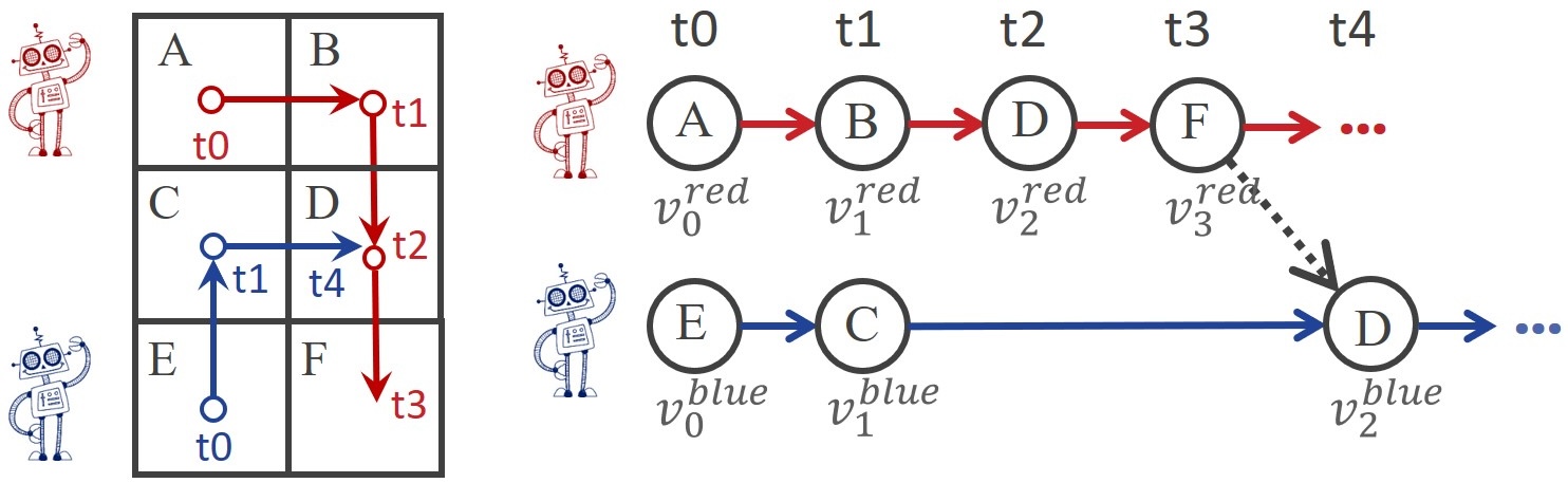
Example 1.
Figure 1 shows an example of converting a MAPF solution into a TPG. Both agents are planned to visit location D, and the red agent is planned to visit D earlier than the blue agent. Consequently, there is a Type 2 edge from to , signifying that the blue agent can move to D only after the red agent has reached F. Note that we define Type 2 edge as instead of to avoid the second type of collision in Definition 1.
Executing a TPG
Procedure 1 describes how to execute a TPG , which includes a main function exec and two helper functions and , along with two marks “satisfied” and “unsatisfied” for vertices. Marking a vertex as satisfied corresponds to moving an agent to the corresponding location, and we do so if and only if all in-neighbors of this vertex have been satisfied. The execution terminates when all vertices are satisfied, i.e., all agents have reached their goal locations. The cost of executing , namely , is the sum of travel time for agents following (while assuming no delays happen).
We now introduce some known properties of TPGs. All proofs are delayed to the appendix. We use to denote a TPG constructed from a MAPF solution as in Definition 3.
Proposition 1 (Cost).
.
Intuitively, if has unnecessary wait actions and otherwise.
Proposition 2 (Collision-Free).
Executing a TPG with Procedure 1 does not lead to collisions among agents.
Next, we present two lemmas regarding deadlocks of executing a TPG, which were used in previous work (Berndt et al. 2020; Su, Veerapaneni, and Li 2024) and are helpful for our discussion of switchable TPGs in the next section.
Definition 4 (Deadlock).
When executing a TPG, a deadlock is encountered iff, in an iteration of the while-loop of Exec(), contains unsatisfied vertices but .
Lemma 3 (Deadlock Cycle).
Executing a TPG encounters a deadlock iff the TPG contains cycles.
Lemma 4 (Deadlock-Free).
If a TPG is constructed from a MAPF solution, then executing it is deadlock-free.
Switchable TPG (STPG)
TPG is a handy representation for precedence relationships. Yet, a TPG constructed as in Definition 3 is fixed and bound to a given set of paths. In contrast, our optimization algorithm will use the following extended notion of TPGs, which enables flexible modifications of precedence relationships.
Definition 5 (STPG).
Given a TPG , a Switchable TPG (STPG) partitions Type 2 edges into two disjoint subsets (switchable edges) and (non-switchable edges) and allows two operations on any switchable edge :
-
•
removes from and add it into . It fixes a switchable edge to be non-switchable.
-
•
removes from and add into . It switches the precedence relationship and then fixes it to be non-switchable.
Remark 3.
Reversing the precedence relationship represented by produces because, based on Definition 3, Type 2 edge indicates locations and are the same. Thus, after reversing, vertex needs to be satisfied before can be marked as satisfied.
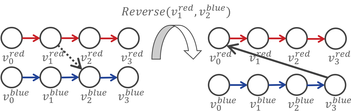
Example 2.
Figure 2 shows an example of reversing an edge. After the operation, edge in the left TPG is replaced with edge in the right TPG.
Definition 5 defines a strict superclass of Definition 3. A STPG degenerates into a TPG if is empty.
Definition 6 (-producible TPG).
Given a STPG , a TPG is -producible if it can be generated through a sequence of and operations on .
We now show the roadmap of our algorithm. Given a MAPF solution , we construct TPG from as in Definition 3 and then run Procedure 1. When a delay happens, we (1) construct a STPG based on and (2) finds a TPG with is -producible, representing an optimal ordering of agents visiting each location, upon sticking to the original location-wise paths. We describe Step (1) below and Step (2) in the next section.
Construction 1.
Assume that, during the execution of , agent is forced to delay at its current location for timesteps. We construct STPG as follows:
-
1.
Construct STPG with is unsatisfied and and is satisfied or .
-
2.
Create new dummy vertices and new Type-1 edges and modify with and .
If there are multiple agents delayed at the same timestep, we repeat Step 2 for each delayed agent.
Remark 4.
In Step 1, is non-switchable when is satisfied because agent has already visited . is non-switchable because agent must be the last one to visit its goal location. The dummy vertices added in Step 2 are used to account for the delays in Procedure 1.
We now show an intuitive yet crucial theorem.
Theorem 5.
If STPG is constructed by Construction 1, then there is at least one deadlock-free -producible TPG.
Proof.
We generate a naïve solution by ing all switchable edges in . Lemma 4 ensures that is deadlock-free. constructed in Step 1 is identical to if we all switchable edges. Step 2 behaves as expanding a pre-existing edge into a line of connecting edges, which does not create any new cycles. Therefore, by Lemma 3, is deadlock-free. ∎
Switchable Edge Search (SES) Framework
We describe our algorithm, Switchable Edge Search (SES), in a top-down modular manner, starting with a high-level heuristic search framework in Algorithm 2. We define the partial cost of a STPG as the cost of its reduced TPG, which is defined as follows.
Definition 7 (Reduced TPG).
The reduced TPG of a STPG is the TPG that omits all switchable edges, denoted as .
Lemma 6.
The partial cost of a STPG is no greater than the cost of any -producible TPG.
Proof.
Let be a -producible TPG. Consider running Procedure 1 on and , respectively. Since an edge appears in must appear in , we can inductively show that, in any call to , if a vertex can be marked as satisfied in , then it can be marked as satisfied in . Thus, the total timesteps to satisfy all vertices in cannot exceed that in . ∎
As shown in Algorithm 2, SES runs A* in the space of STPGs with a root node corresponding to the STPG constructed as in Construction 1. The priority queue sorts its nodes by their -values (namely ). The -value of a node is defined as the partial cost of its STPG. When expanding a node, SES selects one switchable edge in the STPG by module Branch and generates two child nodes with the selected edge being ed or d. We abuse the operators and on Algorithms 2 and 2 to take a STPG and a switchable edge as input and return a new STPG.
SES uses function CycleDetection to prune child nodes with STPGs that definitely produce cyclic TPGs, namely STPGs whose reduced TPGs are cyclic. Specifically, CycleDetection(, returns true iff contains a cycle involving edge . As is acyclic, it holds inductively that CycleDetection(, returns true iff contains any cycle. This is because, when we generate a node, we add only one new non-switchable edge, so any cycle formed must contain the new edge.
Assumption 1.
The modules in SES satisfy:
-
A1
Branch outputs an updated auxiliary information , a value , and a switcable edge of if exists or Null otherwise.
-
A2
Heuristic computes a value such that is the partial cost of for every node .
Theorem 7 (Completeness and Optimality).
Under Assumption 1, SES always finds a deadlock-free TPG with is -producible.
Proof.
First, SES always terminates within a finite time because there are only finitely many possible operation sequences from to any TPG, each corresponding to a node that can possibly be added to . Second, Theorem 5 ensures that there always exist solutions for SES since is constructed as in Construction 1. Therefore, to prove the completeness of SES, we just need to prove the following claim: At the beginning of each while-loop iteration, for any deadlock-free -producible TPG , there exists such that is -producible. Here, we abuse the notation to denote a node in with STPG . This claim holds inductively: At the first iteration, . During any iteration, if some such that is -producible is popped on Algorithm 2, then one of the following must hold:
-
•
contains no switchable edge, i.e., : SES terminates, and the inductive step holds vacuously.
-
•
is -producible: Since is acyclic, so is . Thus, is added into .
-
•
is -producible: This is symmetric to the above case.
In any case, the claim remains true after this iteration. Therefore, SES always outputs a solution within a finite time.
Finally, we prove that the output TPG has the minimum cost. Assume towards contradiction that when is returned, there exists that can produce a better TPG with . Yet this is impossible since Lemma 6 implies that such must have a smaller value and thus would be popped from before . ∎
Execution-based Modules
In this and the next sections, we describe two sets of modules and prove that they satisfy Assumption 1. We start with describing a set of “execution-based” modules in Module 3 and refer to it as Execution-based SES (ESES).
In essence, ESES simulates the execution of the STPG and branches when encountering a switchable edge. It uses to record the index of the most recently satisfied vertex for every agent, indicating their current locations. is updated by the Branch module, which largely ensembles Exec in Procedure 1. At the beginning of each while-loop iteration of Branch, ESES first checks whether the next vertex of any agent is involved in a switchable edge and, if so, returns that edge together with the updated and the cost of moving agents from the old to the new [Algorithms 3 to 3], where the cost is updated inside function Step. If no such edge is found, it runs Step on the reduced TPG to move agents forward by one timestep and repeat the process.
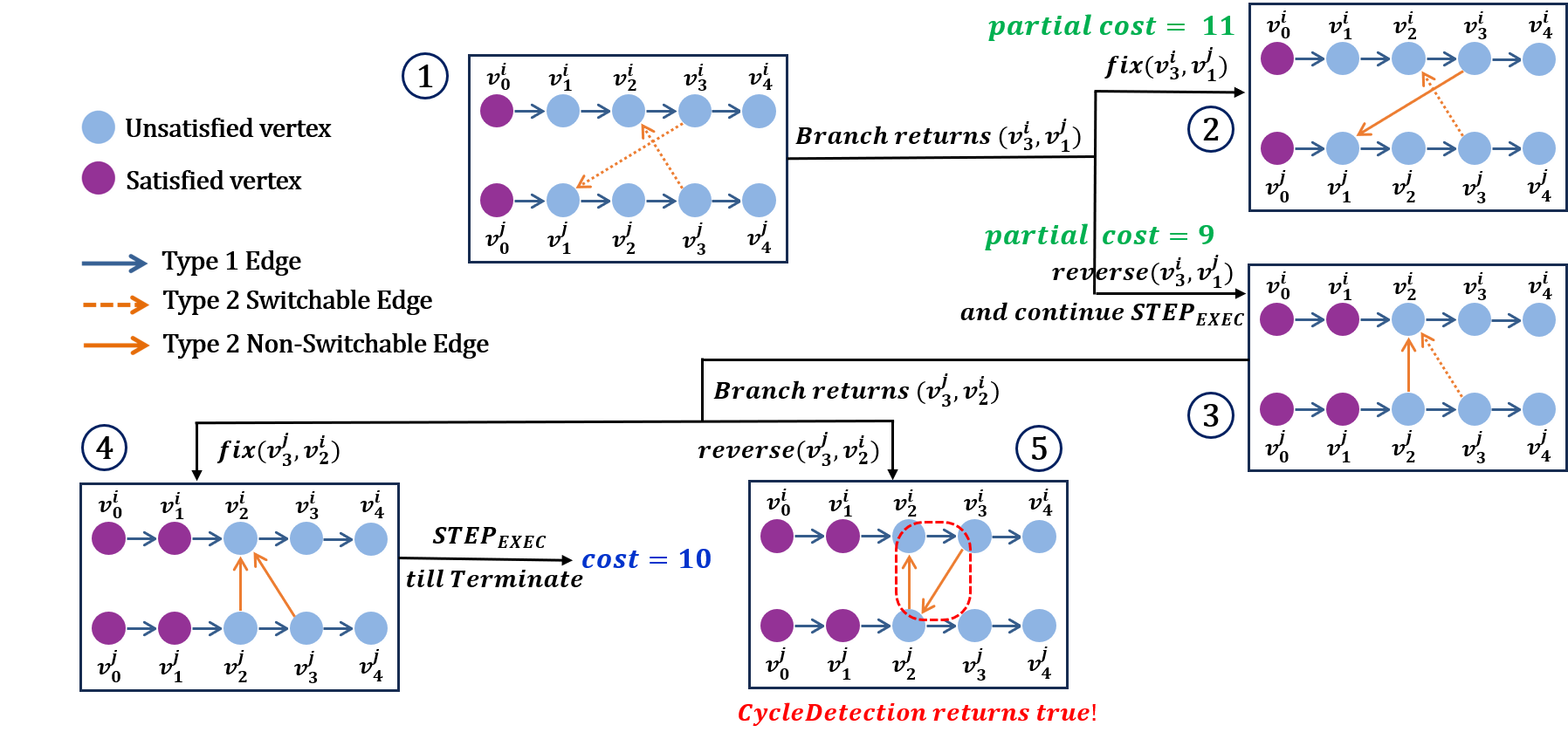
Example 3.
Figure 3 shows an example of ESES.111We note that Figure 3 also works as an example for the GSES implementation in the following section. The only difference is that GSES does not use the notion of “(un)satisfied vertex” or . We start with the top-left STPG ① containing two switchable edges. ESES looks at a “horizon” containing the first unsatisfied vertices and , and then picks the adjacent switchable edge to branch on. This leads to two copies of STPGs ② and ③, containing non-switchable edge or , respectively. ESES expands on STPG ③ first as it has a smaller value. The next switchable edge it encounters is . ESES first es it and generates TPG ④ with , which is the optimal solution. When ESES s the edge, the resulting TPG ⑤ is pruned as it contains a cycle. Note that STPG ② will not be expanded since it has a partial cost greater than the cost of TPG ④.
Proof.
Assumption A1 holds by design. To prove Assumption A2, we first prove the following claim by induction: for every node , is the cost of moving agents from their start locations to . This holds for the root node with and . When we expand a node , returned by Branch is the cost of moving agents from to . Thus, on Algorithms 2 and 2 of Algorithm 2, the value of the child nodes are , which is the cost of moving agents from their start locations to (). So our claim holds. Module heuristic runs function Exec to compute the cost of moving agents from to their goal locations on the reduced TPG, making the partial cost of for every node . ∎
Graph-based Modules
We now introduce an alternative set of modules that focus on the graph properties of a TPG. We refer to this implementation as Graph-based SES (GSES). We will see later in our experiment that this shift of focus significantly improves the efficiency of SES. We start by presenting the following crucial theorem that provides a graph-based approach to computing the cost of a TPG.
Given a TPG and a vertex , let denote the longest path among the longest paths from every vertex to vertex on and denote its length.
Theorem 9.
When we execute a TPG, every vertex is marked as satisfied in the iteration of the while-loop of Exec in Procedure 1.
Proof.
We induct on iteration and prove that all vertices with are marked as satisfied in the iteration. In the base case, are the vertices with and are marked as satisfied in the iteration. In the inductive step, we assume that, by the end of the iteration, all vertices with are satisfied, and all vertices with are unsatisfied. Then, in the iteration, every vertex with is marked as satisfied because all of its in-neighbors have and are thus satisfied. For every vertex with , the vertex right before on , denoted as , has and is thus unsatisfied on Algorithm 1. Thus, every vertex with has at least one in-neighbor unsatisfied and thus remains unsatisfied. Therefore, the theorem holds. ∎
Hence, the last vertex of every agent is marked as satisfied in the iteration, namely the travel time of agent is . We thus get the following corollary.
Corollary 10.
Given a TPG , .
An interesting observation is that, if for a given TPG , then adding edge to does not change its cost since adding does not change any longest paths. We thus get the following corollary that is useful later.
Corollary 11.
Given a STPG , we compute on . For any switchable edge with , ing it does not change the partial cost of .
We adopt the following well-known algorithm to compute on a given deadlock-free TPG : (1) Set . (2) Compute a topological sort of all vertices in . (3) For each vertex in the topological order, we set for every out-neighbor (namely ). The time complexity of this longest-path algorithm is .
With this algorithm, we specify the graph-based modules in Module 4. In GSES, records for every vertex and is updated by the Heuristic module. Since, with , Heuristic can directly compute the partial cost of a given STPG, GSES does not use any values. The Branch module chooses a switchable edge with to branch on. If no such edge exists, then, by Corollary 11, ing all switchable edges produces a TPG with the same cost as the current partial cost. Thus, GSES all such edges and terminates in this case.

Remark 5.
ESES terminates when all vertices are satisfied, which is possible only when all Type 2 edges are non-switchable. This means that ESES has to expand on all switchable edges before getting a solution. In contrast, GSES can have an early termination when ing all switchable edges does not change any longest paths.
Experiment
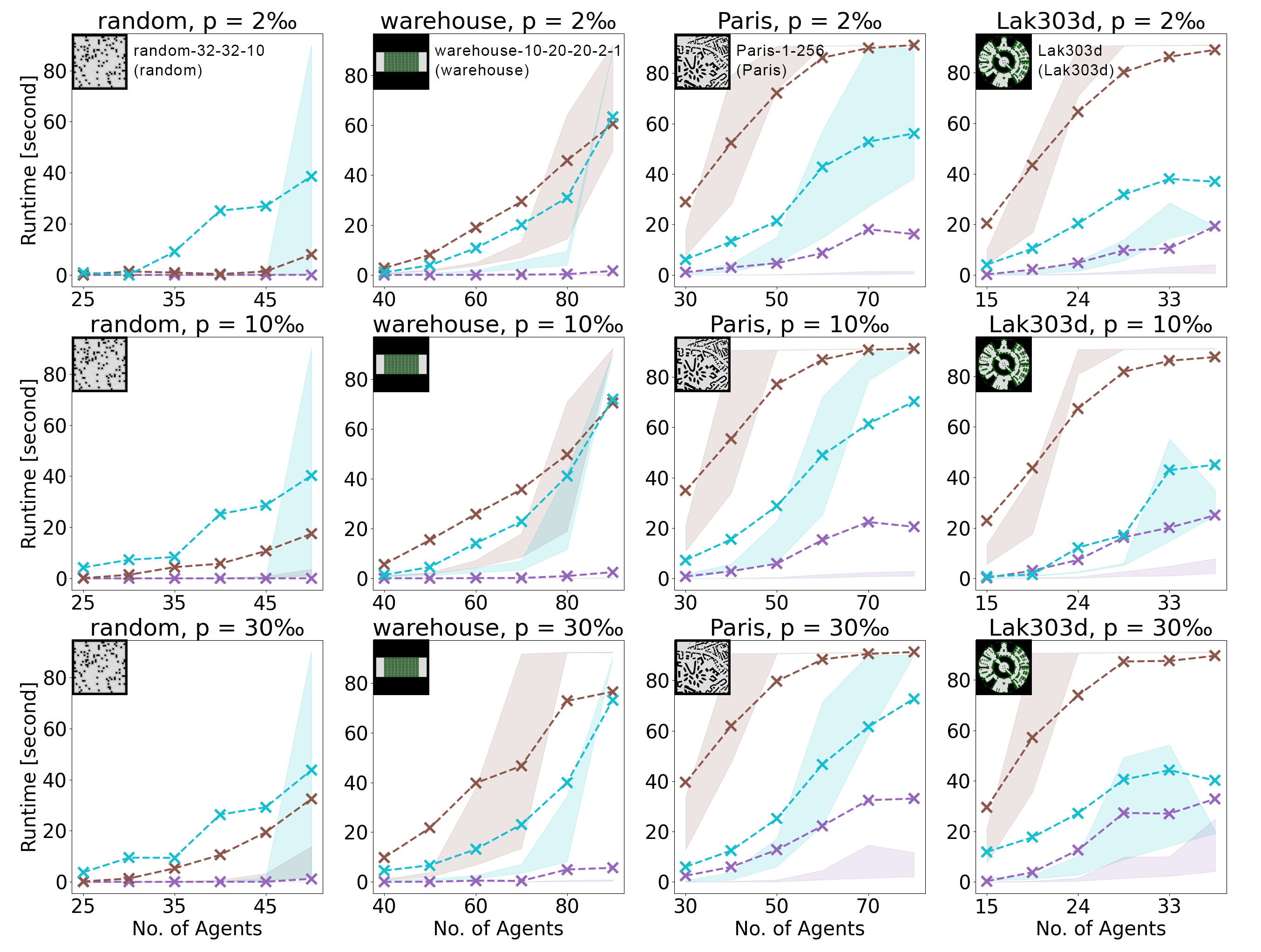
We use maps from the MAPF benchmark suite (Stern et al. 2019), shown in Figure 4, with 6 agent group sizes per map. Regarding each map and group size configuration, we run the algorithms on 25 different, evenly distributed scenarios (start/goal locations) with 6 trials per scenario. We set a runtime limit of 90 seconds for each trial. In each trial, we execute the TPG constructed from an optimal MAPF solution planned by a k-Robust MAPF solver k-Robust CBS (Chen et al. 2021) with . At each timestep of the execution, each agent that has not reached its goal location is subject to a constant probability of delay. When a delay happens, we draw a delay length uniformly random from a range , construct a STPG as in Construction 1, and run our replanning algorithms. We also develop a baseline that uses k-Robust CBS to find the new optimal solution (that takes into account the delay length ) when the delay happens.
We implement all algorithms in C++222Our SES code is available at https://github.com/YinggggFeng/Switchable-Edge-Search. The modified k-Robust CBS code that considers delays is available at https://github.com/nobodyczcz/Lazy-Train-and-K-CBS/tree/wait-on-start. and run experiments on a server with a 64-core AMD Ryzen Threadripper 3990X and 192 GB of RAM.
Efficiency
Figure 4 compares the runtime of ESES and GSES with replanning using k-Robust CBS. In all cases, GSES runs the fastest. Most remarkably, on the random and warehouse maps, the runtime of GSES is consistently below 1 second and does not increase significantly when the number of agents increases, suggesting the potential of GSES for real-time replanning applications.
Comparing ESES and GSES
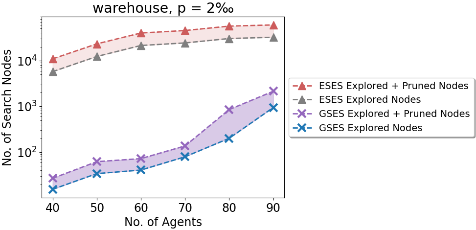
We observe from Figure 4 that, although ESES and GSES adopt the same framework, GSES runs significantly faster than ESES. This is because the longest paths used in GSES defines a simple but extremely powerful early termination condition (see Remark 5), which enables GSES to find an optimal solution after a very small number of node expansions. Figure 5 compares the number of search nodes of ESES and GSES, where explored nodes are nodes popped from the priority queue, and pruned nodes are nodes pruned by CycleDetection. The gap between the red and grey lines (and the gap between the purple and blue lines) indicates the effectiveness of cycle detection for pruning unnecessary search nodes. The gap between the grey and blue lines indicates the effectiveness of early termination as described in Remark 5.
Improvement of Solution Cost
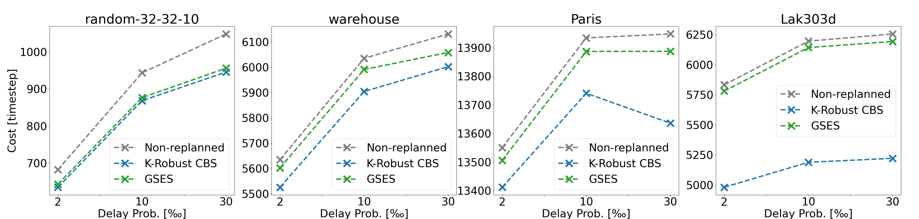
Figure 6 measures the cost of our replanned solution, in comparison to the non-replanned solution produced by the original TPG and the replanned solution produced by k-Robust CBS. We stress that our solution is guaranteed to be optimal, as proven in previous sections, upon sticking to the original location-wise paths, while k-Robust CBS finds an optimal solution that is independent of the original paths. Therefore, the two algorithms solve intrinsically different problems, and the results here serve primarily for a quantitative understanding of how much improvement we can get by changing only the passing orders of agents at different locations. Figure 6 shows that the cost improvement depends heavily on the maps. For example, our solutions have costs similar to the globally optimal solutions on the random map, while the difference is larger on the Lak303d map.
Conclusion
We proposed Switchable Edge Search to find the optimal passing orders for agents that are planned to visit the same location. We developed two implementations based on either execution (ESES) or graph (GESE) presentations. On the random and warehouse maps, the average runtime of GSES is faster than 1 second for various numbers of agents. On harder maps (Paris and game maps), it also runs faster than replanning with a k-Robust CBS algorithm.
Appendix A Appendix: Proofs for Section 3
We rely on the following lemma to prove Proposition 1.
Lemma A.
For every tuple in every path , the corresponding vertex in is satisfied after the iteration of the while-loop of Exec in Procedure 1.
Proof.
We induct on the while-loop iteration and prove that any vertex with is satisfied after iteration . When , this holds because of . Assume that all vertices with are satisfied after iteration . At iteration , for Type 1 edge , is satisfied as . For any Type 2 edge , is also satisfied as by Definition 3. This shows that all in-neighbors of are satisfied after iteration , thus is satisfied after iteration . ∎
Proposition 1 (Cost).
.
Proof.
Lemma A implies that the last vertex of every agent is satisfied after the iteration, i.e., when executing , the travel time of every agent is no greater than . Thus, the proposition holds. ∎
Proposition 2 is similar to Lemma 4 in (Hönig et al. 2016) with different terms. We include a proof for completeness.
Proposition 2 (Collision-Free).
Executing a TPG does not lead to collisions among agents.
Proof.
According to Procedure 1, we need to show that, when a vertex is marked as satisfied [Algorithm 1], moving agent to its location does not lead to collisions. Assume towards contradiction that agent indeed collides with another agent at timestep . Let and be the latest satisfied vertices for agents and , respectively, after the iteration of the while-loop. If and collide because they are at the same location, then , indicating that either edge or edge is in . But this is impossible as neither nor is satisfied.
If they collide because leaves a location at timestep , and enters the same location at timestep , then and are marked as satisfied exactly at the iteration with , indicating that either or is in . But this is also impossible as neither nor was satisfied before the iteration. ∎
Lemma 3 (Deadlock Cycle).
Executing a TPG encounters a deadlock iff the TPG contains cycles.
Proof.
If a TPG has a cycle, executing it will encounter a deadlock as no vertices in the cycle can be marked as satisfied. If executing encounters a deadlock in the iteration of the while-loop, we prove that has a cycle by contradiction. Let denote the set of unsatisfied vertices, which is non-empty by Definition 4. If is acyclic, then there exists a topological ordering of , and must contain the first vertex in the topological ordering as all of its in-neighbors are satisfied, contradicting the deadlock condition of . ∎
Lemma 4 (Deadlock-Free).
If a TPG is constructed from a MAPF solution, then executing it is deadlock-free.
Proof.
If a deadlock is encountered, then the execution would enter the while-loop for infinitely many iterations, and strictly increases in each iteration. Thus, . Yet, is finite, contradicting Proposition 1. ∎
Appendix B Acknowledgement
The research at Carnegie Mellon University was supported by the National Science Foundation (NSF) under Grant 2328671. The views and conclusions contained in this document are those of the authors and should not be interpreted as representing the official policies, either expressed or implied, of the sponsoring organizations, agencies, or the U.S. government.
References
- Atzmon et al. (2020) Atzmon, D.; Stern, R.; Felner, A.; Sturtevant, N. R.; and Koenig, S. 2020. Probabilistic Robust Multi-Agent Path Finding. In Proceedings of the International Conference on Automated Planning and Scheduling, 29–37.
- Atzmon et al. (2018) Atzmon, D.; Stern, R.; Felner, A.; Wagner, G.; Barták, R.; and Zhou, N. 2018. Robust Multi-Agent Path Finding. In Proceedings of the International Symposium on Combinatorial Search, 2–9.
- Berndt et al. (2020) Berndt, A.; van Duijkeren, N.; Palmieri, L.; and Keviczky, T. 2020. A Feedback Scheme to Reorder A Multi-Agent Execution Schedule by Persistently Optimizing a Switchable Action Dependency Graph. ArXiv.
- Chen et al. (2021) Chen, Z.; Harabor, D. D.; Li, J.; and Stuckey, P. J. 2021. Symmetry Breaking for k-Robust Multi-Agent Path Finding. In Proceedings of the AAAI Conference on Artificial Intelligence, 12267–12274.
- Hönig et al. (2019) Hönig, W.; Kiesel, S.; Tinka, A.; Durham, J. W.; and Ayanian, N. 2019. Persistent and Robust Execution of MAPF Schedules in Warehouses. IEEE Robotics and Automation Letters, 1125–1131.
- Hönig et al. (2016) Hönig, W.; Kumar, T. K. S.; Cohen, L.; Ma, H.; Xu, H.; Ayanian, N.; and Koenig, S. 2016. Multi-Agent Path Finding with Kinematic Constraints. In Proceedings of the International Conference on Automated Planning and Scheduling, 477–485.
- Hönig et al. (2018) Hönig, W.; Preiss, J. A.; Kumar, T. K. S.; Sukhatme, G. S.; and Ayanian, N. 2018. Trajectory Planning for Quadrotor Swarms. IEEE Transactions on Robotics, 856–869.
- Kou et al. (2020) Kou, N. M.; Peng, C.; Ma, H.; Kumar, T. K. S.; and Koenig, S. 2020. Idle Time Optimization for Target Assignment and Path Finding in Sortation Centers. In Proceedings of the AAAI Conference on Artificial Intelligence, 9925–9932.
- Ma, Kumar, and Koenig (2017) Ma, H.; Kumar, T. S.; and Koenig, S. 2017. Multi-Agent Path Finding with Delay Probabilities. In Proceedings of the AAAI Conference on Artificial Intelligence, 3605–3612.
- Mannucci, Pallottino, and Pecora (2021) Mannucci, A.; Pallottino, L.; and Pecora, F. 2021. On Provably Safe and Live Multirobot Coordination With Online Goal Posting. IEEE Transactions on Robotics, 37(6): 1973–1991.
- Silver (2005) Silver, D. 2005. Cooperative Pathfinding. In Proceedings of the AAAI Conference on Artificial Intelligence and Interactive Digital Entertainment, 117–122.
- Stern et al. (2019) Stern, R.; Sturtevant, N. R.; Felner, A.; Koenig, S.; Ma, H.; Walker, T. T.; Li, J.; Atzmon, D.; Cohen, L.; Kumar, T. K. S.; Boyarski, E.; and Bartak, R. 2019. Multi-Agent Pathfinding: Definitions, Variants, and Benchmarks. In Proceedings of the International Symposium on Combinatorial Search, 151–159.
- Su, Veerapaneni, and Li (2024) Su, Y.; Veerapaneni, R.; and Li, J. 2024. Bidirectional Temporal Plan Graph: Enabling Switchable Passing Orders for More Efficient Multi-Agent Path Finding Plan Execution. In Proceedings of the AAAI Conference on Artificial Intelligence.
- Wurman, D’Andrea, and Mountz (2007) Wurman, P. R.; D’Andrea, R.; and Mountz, M. 2007. Coordinating Hundreds of Cooperative, Autonomous Vehicles in Warehouses. In Proceedings of the AAAI Conference on Artificial Intelligence, 1752–1759.