Securing GNNs: Explanation-Based Identification of Backdoored Training Graphs

Abstract

Graph Neural Networks (GNNs) have gained popularity in numerous domains, yet they are vulnerable to backdoor attacks that can compromise their performance and ethical application. The detection of these attacks is crucial for maintaining the reliability and security of GNN classification tasks, but effective detection techniques are lacking. Following an initial investigation, we observed that while graph-level explanations can offer limited insights, their effectiveness in detecting backdoor triggers is inconsistent and incomplete. To bridge this gap, we extract and transform secondary outputs of GNN explanation mechanisms, designing seven novel metrics that more effectively detect backdoor attacks. Additionally, we develop an adaptive attack to rigorously evaluate our approach. We test our method on multiple benchmark datasets and examine its efficacy against various attack models. Our results show that our method can achieve high detection performance, marking a significant advancement in safeguarding GNNs against backdoor attacks.

1 Introduction

Graph neural networks (GNNs) [18, 15, 43] have emerged as the mainstream methodology for learning on graph data. A particular GNN task, graph classification, involves predicting the label of a whole graph. This has applications in a variety of domains, such as bioinformatics, social network analysis, and financial services [47, 50]. These domains often involve high-stakes scenarios, highlighting the need to protect GNN models against external threats.

However, backdoor attacks present a significant threat to GNNs. By injecting a predefined trigger into some training graphs, attackers can exert control over the learning capabilities of GNNs. A particular backdoor attack method proposed in [48] has demonstrated significant success in this regard. Specifically, an attacker generates a random subgraph, injects it as a backdoor “trigger” into a small fraction of training graphs, whose labels are changed to an attacker-chosen target label, and uses this backdoored data to train a GNN model. During testing, when a graph is injected with the same subgraph trigger, the backdoored GNN will predict the target label for this backdoored graph.

Limited defenses have been proposed against the backdoor attacks on GNNs. Zhang et al. [48] found that dense-subgraph detection method [16] is not effective. They also designed a provable defense based on randomized subgraph sampling, but their results achieved a zero certified accuracy with a moderate trigger size.

Our defense. To address this shortage, we propose to connect graph-level GNN explanations with backdoored graph detection. Our initial results found the explanatory subgraph outputted by prior GNN explainers can capture certain useful information to help isolate the graph backdoor to some extent. However, it is far inadequate to use the explanatory subgraphs alone for reliably detecting backdoored graphs in GNNs (see Figure 2). This key finding motivates us to design novel metrics, based upon GNN explainers’ output, that can be unified to robustly capture the differences between backdoored and clean graphs. Specifically, we design seven novel metrics, where each metric uncovers certain patterns in explanations of backdoor graphs that differ from those of clean graphs. We then unified them into a single detection method that provides a comprehensive view extending beyond explanatory subgraphs alone. Through evaluations on multiple benchmark datasets and attack models, our method has shown to be consistently effective at distinguishing between clean and backdoor graphs, with an F1 score of up to 0.906 for detection of randomly-generated triggers and 0.842 for detection of adaptively-generated triggers (aim to break our detector). This represents a significant step forward in safeguarding GNNs against backdoor attacks in various applications, especially in high-stakes domains.

Contributions. We summarize our main contribution as below:

• We are the first to use GNN explainers to detect backdoored graphs in GNNs. We show directly applying these explainers is insufficient to achieve the goal.

• To bridge this gap, we introduce a set of novel metrics that leverage valuable insights from certain aspects of the GNN explanation process. These metrics, tested on extensive attack (including adaptive attacks) settings, provide a deeper understanding of the nature of effective graph backdoor attacks.

• We propose a multi-faceted detection method that unifies our metrics. Our method is effective, efficient, and robust to adaptive attacks.

2 Related Work

Backdoor attacks/defenses on non-graph data. Machine learning models for non-graph data, e.g., image [11, 4, 23, 20, 5, 35, 45, 32], text [7, 27, 29, 3], audio [31, 33, 9, 13], video [49], are shown to be vulnerable to backdoor attacks. A backdoored model produces attacker-desired behaviors when a trigger is injected into testing data. Gu et al. [11] propose the first backdoor attack, called BadNet, on image classifiers. BadNet injects a trigger (e.g., a sticker) into some training images (e.g., “STOP" sign) and changes their labels to the target label (e.g., “SPEED" sign). An image classifier trained on the backdoored training set then predicts the target label for a testing image when the trigger is injected into it, e.g., classify a “STOP" sign with a “sticker" to be the “SPEED" sign.

Many empirical defenses [4, 23, 24, 21, 38, 8, 22, 14, 39, 26] have been proposed to mitigate backdoor attacks. For instance, Wang et al. [38] proposed Neural Cleanse to detect and reverse engineer the trigger. However, all these defenses are broken by adaptive attacks [41]. These two works [37, 41] proposed provable defenses against backdoor attacks in the image domain. However, they are shown to have limited effectiveness against backdoor attacks.

Backdoor attacks/defenses on graph data. A few works [48, 42] have studied backdoor attacks on GNNs. Zhang et al. [48] were the first to find that GNNs are vulnerable to backdoor attacks. Specifically, they introduced a subgraph as a trigger, where the subgraph is generated by three models (i.e., the Erdős-Rényi (ER) [10], Small World (SW) [40], and Preferential Attachment (PA) models [1]). The attack then injects a random subgraph into a set of clean training graphs, where attached nodes within these graphs are randomly selected, and the labels of these backdoored graphs are set to an attacker-chosen target label. After training, the backdoored model will behave normally on clean graphs, but predict the target label for those with a subgraph trigger. Instead of using a random subgraph as the trigger, Xi et al. [42] proposed optimizing the subgraph trigger and finding the most vulnerable nodes in a graph to be attached. Nevertheless, the two attacks were shown to have similar performance [12].

Limited defenses have been proposed against the graph backdoor. [48] found dense-subgraph based subgraph trigger detection method [16] is ineffective. It then proposed a provable defense based on randomized subgraph sampling. The defense ensures a trained (backdoored) GNN model provably predicts the correct label for a testing graph once the injected subgraph trigger has a size less than a threshold (which is called certified trigger size). However, their results show the defense has zero certified accuracy when the trigger size is moderate to large.

3 Background and Problem Definition

3.1 GNNs and Backdoor Attacks

GNNs for graph classification. Given a graph $G=(\mathcal{V},\mathcal{E})$ with node set $\mathcal{V}$ and edge set $\mathcal{E}$, and its label $y\in\mathcal{Y}$, a graph classifier $f$ takes the graph $G$ as input and outputs a label $\hat{y}$, i.e., $f:G\rightarrow\mathcal{Y}$. A GNN-based graph classifier iteratively learns a node representation via aggregating the neighboring nodes’ representations, and the last layer outputs a label for the graph. To train the GNN, we are given a set of (e.g., $n$) training graphs $\mathcal{D}^{tr}$=$\{(G_{1},y_{1}),(G_{2},y_{2}),\cdots,(G_{n},y_{n})\}$, where $G_{i}$ and $y_{i}$ are the $i$th training graph and its true label, respectively. Stochastic gradient descent is often used to train the classifier. The trained model $f$ is used to predict labels for testing graphs.

Backdoor attacks to GNNs. An attacker injects a subgraph/backdoor trigger to a fraction of training graphs and changes their labels to be the attacker-chosen target label, e.g., $y^{t}$. The training graphs with the injected subgraph are called backdoored training graphs. A GNN classifier trained learned on backdoored graphs is called a backdoored GNN. The backdoored GNN aims to memorize the relation between the target label and the subgraph trigger. Hence, when the attacker injects the same subgraph into a testing graph, the backdoored GNN predicts the target label for the backdoored testing graph with high probability.

3.2 GNN Explanation

Suppose we have a well-trained GNN model $f$ for graph classification, a graph $G$, and its prediction by $f$. The goal of GNN explanation is identifying an explanatory subgraph of the original graph, $G^{S}=(\textbf{M}^{\mathcal{V}}\otimes\mathcal{V},\textbf{M}^{\mathcal{E}}\otimes\mathcal{E})\subset G$, that preserves the information guiding $f$ to its prediction. Here, we denote the prediction of $f$ on $G^{S}$ as $f(G^{S})=\hat{y}^{S}$, $\otimes$ means the element-wise product, $\textbf{M}^{\mathcal{V}}\in[0,1]^{|\mathcal{V}|}$ and $\textbf{M}^{\mathcal{E}}\in[0,1]^{|\mathcal{E}|}$ are called node mask and edge mask, respectively. In general, the objective function of a GNNExplainer is to optimize the two masks as below:

$$\small\min_{\textbf{M}^{\mathcal{V}},\textbf{M}^{\mathcal{E}}}L(y,\hat{y}^{S})+R(\textbf{M}^{\mathcal{V}},\textbf{M}^{\mathcal{E}}),$$ (1)

where $L$ is an explainer-dependent loss (e.g., cross-entropy loss), and $R$ is a regularization function on the masks. For instance, the objective function of the well-known GNNExplainer [46] is defined as

$$\small\min_{\textbf{M}^{\mathcal{V}},\textbf{M}^{\mathcal{E}}}L(y,\hat{y}^{S})+\boldsymbol{\lambda}\cdot\left(\left\|\textbf{M}^{\mathcal{E}}\right\|+\left\|\textbf{M}^{\mathcal{V}}\right\|+H(\textbf{M}^{\mathcal{E}})+H(\textbf{M}^{\mathcal{V}})\right),$$ (2)

where $H(\cdot)$ is the entropy function.

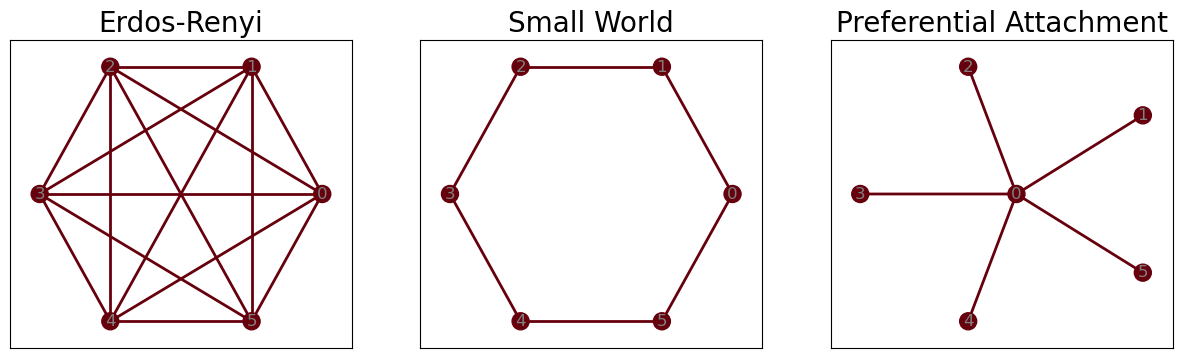
Figure 1: Samples of the types of triggers used in our analysis.

3.3 Threat model

We define our threat model by the attacker’s goal, capability, and trigger design.

• Attacker’s goal: It results in the prediction of the target label for samples containing the trigger. Accuracy should remain high for clean samples, but should “flip” the prediction on backdoored samples with a high success rate.

• Attacker’s capability. The attacker is able to modify the training data and change the ground truth label. This allows for the injection of backdoor triggers into particular samples, and for the attacker to change the ground truth label of those samples to the target label.

• Attacker’s trigger design. The attacker has free choice over the structure and placement of the trigger subgraph. We implement two types of attacks. First, we used randomized trigger generation using one of three models – Erdős-Rényi (ER) [10], Small World (SW) [40], and Preferential Attachment (PA) [1]) (See Figure 1). We assume each trigger node is randomly mapped to an existing node in the original graph, and any existing connections between those nodes are replaced by the edges in the trigger subgraph. Second, we implemented an adaptive attack using a trigger generation process that attacks our detection method (See details in Section 4.4).

Design goal. We aim to detect backdoor samples in the training graphs under the threat model. We assume that we have access to both the training graph, $\mathcal{D}^{tr}$, and a set of clean graphs that we can use for validation purposes, $\mathcal{D}^{val}$.

4 Method

4.1 Limitations of GNN Explainers for Backdoor Detection

In the backdoor attack on GNNs [48], a trigger subgraph is injected into the original (clean) graph, tricking a GNN into predicting the attacker-chosen target label. Since a GNN explainer outputs a subgraph as an explanation, our initial instinct was to check whether such an explanation would reveal the trigger in a backdoored graph. However, this strategy has its limitations.

Limited capability of explanatory subgraph to detect trigger.

Indeed, we found explanation masks $\textbf{M}^{\mathcal{E}}$ and $\textbf{M}^{\mathcal{V}}$ could preserve some backdoored edges and nodes in the resulting subgraph. However, in some instances, they failed to produce any understandable patterns. Inconsistencies were prominent across different datasets, GNN models, and especially explanation methods. For instance, we also tested PGExplainer [25]. Once again, success was limited and inconsistent (see examples in supplementary material). These issues highlight the limitations of relying solely on explanatory subgraphs to detect backdoored graphs.

Despite these inconsistencies, Figure 2 demonstrates GNNExplainer’s ability to capture some useful information. In the MUTAG example, the trigger nodes were the only ones preserved by $\textbf{M}^{\mathcal{V}}$, and all six trigger edges were preserved by the $\textbf{M}^{\mathcal{E}}$. In the PROTEINS example, five of six trigger edges are preserved, in addition to all four trigger nodes, but additional edges and nodes are also preserved. In the DBLP example, all trigger nodes are preserved, but only one of the six trigger edges is. However, taken collectively, the five examples in Figure 2 still demonstrate that GNNExplainer is able to identify backdoor features to a degree.

Multi-faceted approach. While $G^{S}$ is insufficient to reveal full backdoor information, we found that considering an explanation from multiple aspects yielded more consistent detection results. In particular, we found that seven novel metrics generated as byproducts of the explanation process were successful in distinguishing between clean and backdoor explanations.

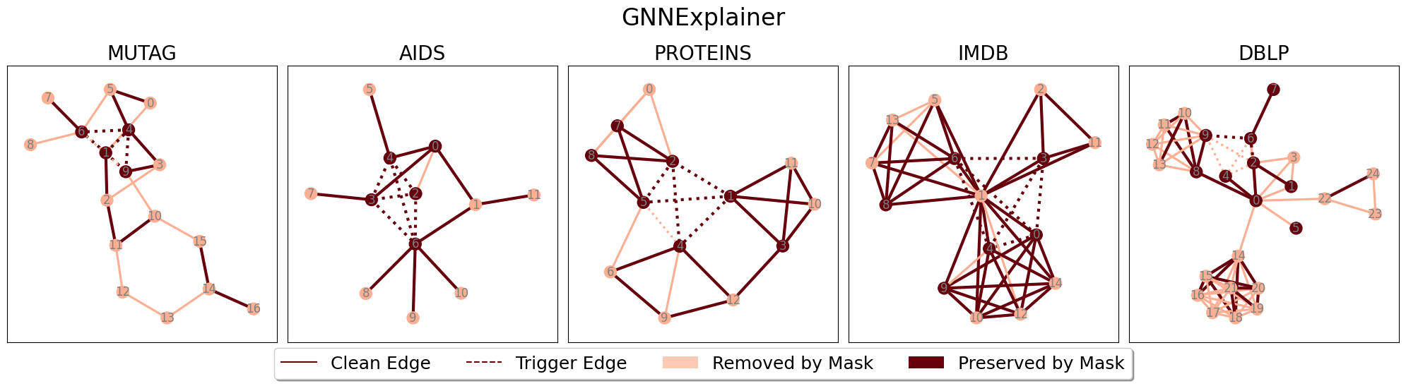
Figure 2: GNNExplainer results on a backdoored graph from each dataset. We observe the performance of the explanation— particularly the ability to isolate the trigger—was inconsistent across examples. Such phenomenon also exists across different explainers – see supplementary for examples.

4.2 Our Proposed Metrics

Our metrics do not solely rely on the subgraphs that have been uncovered. We note that signs of the backdoor are present across different learning stages of the explanation process, and our novel detection metrics are derived from their varied artifacts. Particularly, the explainer loss curve, the predicted probabilities for each class provided by the explainer, and the explanation masks all help to define the characteristics of the input. By collectively leveraging all metrics, we aim to achieve a detection method that is both more effective and robust. Below, we will detail these metrics and the rationale behind each one.
Prediction Confidence. The maximum predicted probability for a testing graph. We hypothesize this probability will be larger for backdoored graphs, since the backdoor trigger is a more robust pattern than the diverse clean graphs and the model has learned it with high certainty.
Explainability. Inspired by [28, 17], we define explainability as the difference between positive fidelity ($\text{fid}_{+}$) and negative fidelity ($\text{fid}_{-}$).

$$\text{Explainability}=\text{fid}_{+}-\text{fid}_{-},$$ (3)

Fidelity can be thought of as the degree to which the original GNN classification model depends on the explanatory subgraph $G^{S}$. $\text{fid}_{-}$ measures the degree to which the model’s prediction changes when only $G^{S}$ is considered, while $\text{fid}_{+}$ measures the effect when $G^{S}$ is excluded. For backdoored samples, given that $G^{S}$ should contain essential backdoor information, its exclusion will likely be costly for the explainer. We expect the exclusion of $G^{S}$ to have a smaller effect for clean explanations, since its contribution to the predicted class is less likely to be confined to a single subgraph. Extending this logic, excluding the complement of $G^{S}$, i.e., $G^{C}=G-G^{S}$, should come at a low cost for backdoor explanations, since the remaining $G^{S}$ is expected to contain trigger information central to the model’s prediction. Conversely, for clean explanations, $G^{C}$ is still likely to contain some helpful information for class prediction. Specifically, these terms are defined as follows:

$$\text{fid}_{+}=\lvert d\left(\hat{\textbf{p}},\textbf{y}\right)-d(\hat{\textbf{p}}^{C},\textbf{y})\rvert,\quad\text{fid}_{-}=\lvert d\left(\hat{\textbf{p}},\textbf{y}\right)-d(\hat{\textbf{p}}^{S},\textbf{y})\rvert,$$ (4)

where $\hat{\textbf{p}}$, $\hat{\textbf{p}}^{C}$, and $\hat{\textbf{p}}^{S}$ indicate the probability vector outputted by the GNN model on the graphs $G$, $G^{C}$, and $G^{S}$, respectively; and y is the one-hot (true) label of $G$. $d$ is a distance function, e.g., Euclidean distance in our results. We expect backdoored graphs to have higher $\text{fid}_{+}$ and lower $\text{fid}_{-}$ than their clean counterparts. We therefore predict that explainability score will be higher for backdoor graphs.

Connectivity. A measurement of the proximity and connection of nodes in $G^{S}$. Given that the triggers are a single connected graph, an explanation revealing the trigger should be, too. This metric can be interpreted as the proportion of node pairs in the subgraph with edges between them in the original graph.

$$\text{Connectivity}=\frac{1}{|\mathcal{V}^{S}|}\sum_{(i,j)\in\mathcal{V}^{S}}\mathbbm{1}\{(i,j)\in\mathcal{E}\}$$ (5)

where $|\mathcal{V}^{S}|$ is the number of nodes preserved in the explanatory subgraph of a particular graph, and $\mathbbm{1}\{(i,j)\in\mathcal{E}\}$ is an indicator meaning whether nodes $i$ and $j$ are in the set of edges in the original graph.

Subgraph Node Degree Variance (SNDV). The variance of the node degrees within $G^{S}$. With the attack proposed by Zhang et al, [48], the node features are set to their degree. Therefore, we hypothesize that the distribution of node degrees within the trigger should be unique for the classifier to learn the degree as a distinct feature, i.e., for the attack to be successful. Extending this logic, if $G^{S}$ contains the trigger, we expect its node degree distribution to be different than those observed in clean subgraphs. This metric can be computed as:

$$\text{SNDV}=\text{var}(\{\text{deg}(v_{i})^{S}|i\in\{1,2,\dots,|\mathcal{V}^{S}|\}).$$ (6)

where $\text{deg}(v_{i})^{S}$ denotes the degree of the $i^{th}$ node in $G^{S}$, and $|\mathcal{V}^{S}|$ denotes the number of nodes in $G^{S}$.

Node Degree Variance (NDV). This is the only metric that solely depends on the geometry of the original graph rather than the explanation. Specifically, it is defined as the variance of node degrees within a graph:

$$\text{NDV}=\text{var}(\{\text{deg}(v_{i})|i\in\{1,2,\dots,|\mathcal{V}|\}).$$ (7)

The logic for including this metric is similar to that of SNDV, where the core idea is that attack success correlates with node degree variance. If this is the case, then a successful attack can be expected to change the node degree distribution of the graph as a whole. Moreover, if the trigger is inserted at random nodes, the selected nodes are not often in close proximity to each other. As a result, trigger injection often adds edges between nodes that were previously disconnected, thereby increasing the degrees of those nodes and potentially increasing the range of node degrees presented in the graph. Therefore, random node insertion often has the effect of increasing node degree variance.

Elbow. The epoch at which loss curve $L$’s rate of decrease significantly changes:

$$\text{Elbow}={t_{e}=\arg\max_{t\leq t_{\max}}\left\{L_{t}-L_{t+1}\right\}},$$ (8)

where $L_{t}$ and $L_{t+1}$ are loss values at the $t$ and $t+1$ iterations, and $t_{max}$ is the maximum number of epochs. We hypothesize that in the case of a strong attack, the backdoor trigger will be easy for the explainer to identify; as a result, explainer loss should converge more quickly for backdoored graphs than for clean graphs, resulting in a smaller elbow epoch.

Curvature. A measurement of the sharpness, or magnitude of change, at the elbow of loss curve $L$. We hypothesize that the decision boundary between the non-target and target class will be sharper when the trigger is present. Consequently, this will be larger for backdoored graphs.
Curvature is traditionally defined as $L^{\prime\prime}_{t_{e}}/{\left(1+(L^{\prime}_{t_{e}})^{2}\right)^{\frac{3}{2}}}$. However, for our discrete loss curve, its exact curvature is tricky. Here, we instead use a proxy from the normalized loss curve, $\tilde{L}$, which is the result of applying a post-normalization on the loss $L$ defined as: $\tilde{L}=\frac{L-\min(L)}{\max(L)-\min(L)}$. We then define curvature as:

$$\text{Curvature}=\tilde{L}_{elbow},$$ (9)

where $\tilde{L}_{elbow}$ represents the y-coordinate at its elbow. This specific value, provides a measure indicative of the most pronounced inflection in the loss.

Caveat for loss curve metrics: Note that our expectations for Elbow and Curvature change with smaller trigger sizes, which correspond to weaker attacks: rather than Elbow being lower and Curvature being higher for backdoored graphs versus their clean counterparts, we observe the opposite when the trigger size is 2. However, we emphasize that, regardless of the value order of these two metrics, we still found a distinct separation of clean graphs and backdoored graphs. Due to this caveat, our use of loss curve metrics in backdoor detection differs from our use of other metrics. We discuss this further in the next section.

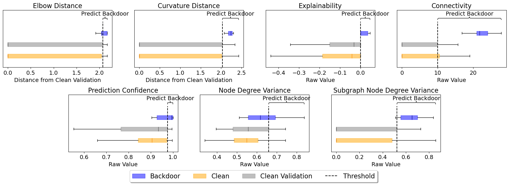
Figure 3: Detection metric distributions from a single dataset (MUTAG), attack (PA trigger size 4 in 20% of training data), and model (GIN architecture [43]). The figure represents 72 graphs (28 clean validation, 30 clean training, 14 backdoor training), and exemplifies varied metric effectiveness both within a dataset and across metric types. This single example is not indicative of all instances – see supplementary for more.

4.3 Detection Strategy

Clean validation extrema as prediction threshold. We can establish expected distributions for clean values by computing each of the above metrics on $\mathcal{D}^{val}$. We expect clean graphs in $\mathcal{D}^{tr}$ to align with this distribution, but backdoored graphs in $\mathcal{D}^{tr}$ to have a distinct distribution. $\mathcal{D}^{val}$ can be used to establish a threshold to predict whether or not a graph is clean or backdoored. If a metric is expected to produce larger values for backdoored graphs, we set the threshold to a high percentile of $\mathcal{D}^{val}$ metric values. In our experiments, we have used the 75th percentile for this case. Conversely, if the metric is expected to produce smaller values for backdoored graphs, we set the threshold to be a small percentile of all $\mathcal{D}^{val}$ metric values. In our experiments, we used the 25th percentile for this case. Figure 3 provides an example of the metric distributions for clean and backdoored graphs in the MUTAG dataset, and illustrates how we define the threshold for backdoor detection.

As mentioned, this method differs for loss curve metrics, which were more sensitive to attack strength than the others. As a result, before using the above thresholding method, we first transform loss metric values to their normalized distance from the clean validation distribution:

$$m_{i}^{j}=\frac{m^{j}(\mathcal{D}_{i}^{tr})-\overline{m^{j}}(\mathcal{D}^{val})}{\sigma\big{(}m^{j}(\mathcal{D}^{val})\big{)}}$$ (10)

where $m^{j}(\mathcal{D}_{i}^{tr})$ represents the $j$-th metric generated for the $i^{th}$ training sample, and $\overline{m^{j}}(\mathcal{D}^{val})$ and $\sigma\big{(}m^{j}(\mathcal{D}^{val})\big{)}$ are the mean and standard deviation of the corresponding metric on the clean validation data, respectively. We can therefore define each metric from two perspectives:

• Raw metric: The metric value defined in Section 4.2.

• Distance metric: The distance of a metric value from clean-validation counterparts, as defined in Equation (10).

Since instances of reversed expectations only occurred on loss curve metrics, we use the distance versions of Curvature and Elbow, but the raw versions of Prediction Confidence, Explainability, Connectivity, SNDV, and NDV.

Composite metric. While no single metric is foolproof, considering multiple metrics at a time can boost our confidence in our detection. As a result of clean validation thresholding, each metric casts a vote for whether an incoming sample is clean or backdoor. Consider the following definitions:

• Positive metric: A metric value following backdoor expectations, surpassing the threshold (i.e., the 25th/75th percentile) of the clean validation values.

• Negative metric: A metric value following clean expectations, not surpassing the threshold (i.e., the 25th/75th percentile) of clean validation values.

Our composite metric uses this notion of positive and negative metrics to make a final prediction of clean or backdoor. For an individual graph, if a minimum of $k$ out of the seven metrics are positive, then we classify it as a backdoor. Moving forward, we refer to this arbitrary $k$ as the Number of Positive Metrics Required, or NPMR, for short. We have determined that NPMR between 2 and 4 yields favorable outcomes. For more details, please refer to Section 5.

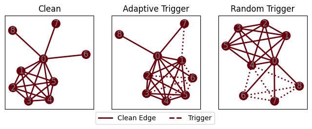
Figure 4: The graph with the adaptive trigger is much more faithful to the original structure than its random trigger counterpart.

4.4 Adaptive Backdoor Trigger

Since our metrics are derived directly from the explanation process (with the exception of Node Mask Variance), a backdoor attack that evades GNN explanation has the potential to evade detection by our combined metric. Based on this observation, we propose an attack that simultaneously targets the GNN classification model and the explanation process.

The key idea is two-fold: (1) train a generator GNN to produce triggers that evade GNN explanation, and (2) simultaneously train the target GNN model that minimizes classification loss on the backdoored graphs with the trigger produced by this generator. The adaptive attack follows the process below:

• Pre-train a surrogate GNN graph classifier on a clean graph dataset.

• Begin with untrained edge generator GNN.

• Iteratively repeat the following process:

  • Use edge generator to add the trigger to clean graphs.

  • Obtain explanation of current classifier’s prediction on triggered graphs.

  • Perform gradient descent on generator using objective function (11).

  • Retrain the graph classifier such that classification loss is minimized on the triggered dataset.

• Use the trained edge generator to attack unseen testing graphs.

We now describe key step (c) in more detail. For ease of description, we momentarily change the notation to represent edges with adjacency matrix A rather than the set $\mathcal{E}$. Conceptually, $\textbf{M}^{A}$ is the same as explanatory mask $\textbf{M}^{\mathcal{E}}$, $\hat{\textbf{A}}$ is the adjacency matrix corresponding to a backdoored graph, and B is the mask for edges not in the clean graph. Formally, we have:

$$\min_{\hat{A}}\sum\textbf{M}^{\hat{A}}\odot\textbf{B}.$$ (11)

$\textbf{M}^{\hat{A}}\odot\textbf{B}$ represents the explanatory mask weights corresponding to the new edges. The key intuition is that edges with small explanatory mask weights will be “left out” of the explanatory subgraph. Therefore, objective function 11 works by iteratively training the edge generator to produce trigger edges in $\hat{\textbf{A}}$ that the GNN explainer deems unimportant.

This process yields a stealthy trigger that blends in with the geometry of the clean graph, as seen in Figure 4. See supplementary for more details about the implementation of this type of attack.

5 Experiments

5.1 Experimental Setup

5.1.1 Datasets and attack models.

We used five widely studied graph datasets in our assessment. MUTAG [6] is a set of graphs representing chemical compounds according to their mutagenic effect. AIDS [30] contains graphs of molecular structures tested for activity against HIV. PROTEINS [2] includes structures categorized as enzymes or non-enzymes. IMDB-BINARY [44] is a movie collaboration dataset consisting of actors’ ego-networks, with each graph labeled as a movie genre (Action or Romance). DBLP [34] is a citation network indicating whether a paper belongs to database & data mining or computer vision & pattern recognition fields. For attack models, we follow the random backdoor attacks in [48] (see Section 3.3) and the adaptive backdoor attack outlined in Section 4.4.

Parameter settings. Several notable hyperparameters could affect the performance of both our attacks and detection methods. We diversified our attacks by varying these trigger type and size, using random and adaptive triggers of sizes 2 through 12. For random attacks, we also varied the probability that trigger nodes are interconnected, using probabilities of 1%, 50%, or 100%. Poisoning ratio was held constant at 20% of training data, ensuring the attack is strong (the maximum ratio used by Zhang et al. [48] is 10%). We used uniform random sampling to select which graphs to include in this subset.

We primarily used GCN [18], GIN [43], and GAT [36] in the construction of our graph classifiers. Our varied datasets and attacks required varied models – our classifiers each consisted of 2 to 4 layers, had between 16 and 256 hidden dimensions, and were trained between 150 and 600 epochs.

GNNExplainer’s most notable hyperparameters are the coefficients of its loss components – edge mask entropy, node mask entropy, edge mask size, and node mask size. We held these values constant at 1.0, 1.0, 0.0001, and 0.0001 – respectively – across experiments.

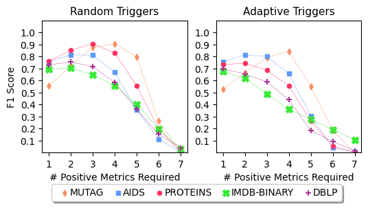
Figure 5: Results obtained using the composite metric, across datasets and trigger types. The y-axis shows the F1 score when applying each NPMR as the detection rule. An NPMR of 1 identifies many backdoor instances but at the cost of more false positives and fewer true negatives. Conversely, an NMPR of 7 fails to detect almost all backdoor instances. F1 peaks around 2 or 3 NPMR in most cases. While adaptive triggers are better at evading our method, detection of adaptive triggers is still respectable.

5.2 Experimental Results

Impact of NPMR on F1 score. Each attempt to detect backdoor triggers with a specific NPMR yields a confusion matrix. By comparing these confusion matrices, we can choose the optimal requirement for backdoor prediction. Figure 5 shows the result. Each curve represents the average F1 scores at different NPMRs across 529 unique random attacks and 85 adaptive attacks. For adaptive attacks, the composite score peaks at 2 NPMR in the average case, with an F1 score of 0.727. For random attacks, composite scores peak at 3 NPMR in the average case, with an F1 score of 0.794 – however, 2 NPMR yields an F1 score of 0.782, which is still strong. Therefore, an NPMR of 2 generalizes well across attack types and datasets. Table 1 shows the specific breakdown of these values.

Table 1: Detection performance, across all trigger types, with respect to varied levels of NPMR. An ideal NPMR should yield high F1 score, a high TPR, and a low FPR.

		NPMR
	Dataset	1	2	3	4	5	6	7
Random
	All	0.718	0.782	0.794	0.696	0.460	0.169	0.017
	MUTAG	0.555	0.722	0.876	0.906	0.799	0.263	0.013
	AIDS	0.757	0.815	0.813	0.671	0.356	0.113	0.007
	PROTEINS	0.760	0.852	0.908	0.830	0.559	0.200	0.005
	IMDB-BINARY	0.695	0.704	0.648	0.557	0.402	0.199	0.031
	DBLP	0.731	0.756	0.717	0.586	0.362	0.154	0.040
Adaptive
	All	0.694	0.727	0.700	0.591	0.314	0.099	0.026
	MUTAG	0.526	0.664	0.793	0.842	0.552	0.186	0.000
	AIDS	0.755	0.815	0.801	0.659	0.307	0.041	0.006
	PROTEINS	0.733	0.747	0.686	0.558	0.264	0.053	0.003
	IMDB-BINARY	0.680	0.618	0.490	0.361	0.278	0.193	0.106
	DBLP	0.697	0.657	0.590	0.440	0.184	0.092	0.016

Effectiveness against adaptive attacks. Figure 5 and Table 1 illustrate that in most cases, our detection strategy performs better against random backdoor attacks than adaptive ones. This can be seen in two ways. First, given the optimal choice for NPMR, the average detection attempt against a random attack has an F1 score of 0.794, whereas the F1 score is 0.727 in an average adaptive attack. Moreover, unlike random attacks, the F1 score for adaptive attacks decreases significantly after an NPMR of 2, indicating that we cannot expect as many individual metrics to simultaneously “tell the truth”. However, these two points aside, we emphasize that the composite metric still performs reasonably well in the adaptive case, suggesting that our composite detection method is robust against attacks on our individual metrics.

5.3 Ablation Studies

5.3.1 Relationship between attack strength and detection.

Figure 6 plots F1 scores for detection against trigger size and attack success rate. In this context, attack success rate (ASR) is the portion of the testing backdoored graphs that the GNN model misclassified them as the target label. These trends indicate that our composite metric performs best when trigger size is larger and ASR is higher. This is consistent with our observation in Section 4.2 that the reliability of some metrics depended on attack strength. These results suggest that stronger attacks may be easier to detect.

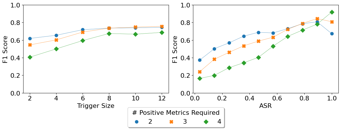
Figure 6: F1 scores under different trigger sizes and attack success rates using our composite metric. Each subplot further shows how these trends vary for NPMR ranging between 2 and 4. Both trigger size and attack success rate are positively correlated with the performance of our composite metric.

Prevalence of individual metrics in k-sized positive sets. Figure 7 shows the percentage of all detection attempts where a given metric is among $k$ positive metrics, thereby quantifying that metric’s influence in predicting backdoor for different NPMR. For example, the second row indicates that Prediction Confidence is among exactly two positive metrics only 9.1% of the time, whereas it is among 4 positive metrics 19.7% of the time. This indicates that the contributions of each metric are not consistent across NPMR.

Impact of clean validation thresholding on best NPMR. As mentioned in Section 4.3, we used the 25th/75th percentile of the clean validation data to establish the thresholds for making a positive prediction for individual metrics. Table 2 shows how the optimal NPMR changes under different thresholding settings. (Note that the “Percentile” refers to the upper percentile for a given configuration – for example, “95” indicates a lower and upper threshold at the 5th and 95th percentile, respectively.) We see that NPMR decreases as the threshold upper percentile increases. Consider the 50th percentile threshold, which yields a backdoor prediction for an individual graph if a given metric surpasses the median of clean validation values. We have little faith in this prediction, since the threshold will predict 50% of the clean validation itself to be backdoor. We will be more convinced of this prediction if many individual metrics “agree” – therefore, it is reasonable that the optimal NPMR is 5 in this instance. Conversely, a value surpassing a threshold at the 100th percentile of clean validation values is more convincing as a potentially-backdoored sample, and a single positive metric is enough for a confident backdoor prediction.

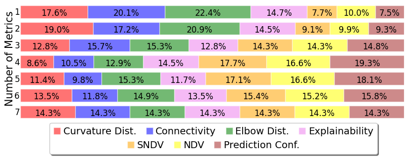
Figure 7: The rate at which each metric is included among exactly $k$ positive metrics. Measured across all datasets and attack types.

Table 2: Optimal NPMRs at varying clean validation thresholds. For a 25th/75th percentile threshold, this value is 3 for random attacks and 2 for adaptive attacks.

			Percentile
Trigger Type	50	55	60	65	70	75	80	85	90	95	100
ER	5	4	4	4	3	3	2	2	1	1	1
SW	4	4	4	3	3	3	2	1	1	1	1
PA	4	4	4	3	3	3	2	1	1	1	1
Adaptive	4	4	3	3	3	2	1	1	1	1	1

6 Conclusion

In this paper, we explore the vulnerabilities of Graph Neural Networks (GNNs) to backdoor attacks and the challenges in detecting these intrusions. Our research highlights the limitations of simply using existing GNN explainers, such as GNNExplainer and PGExplainer, in consistently revealing the full scope of backdoor information. Although these explainers can sometimes capture significant aspects of the backdoor trigger, their success is not uniform and often includes clean parts, leading to inconsistencies and incompleteness in detection.

To address these limitations, we propose a novel detection strategy that collectively leverages seven new metrics, offering a more robust and multifaceted approach for backdoor detection. The effectiveness of our method has been demonstrated through extensive evaluations on various datasets and attack models.

Acknowledgments. This work was supported by the National Science Foundation under grant Nos. 2319243, 2216926, 2331302, 2241713, and 2339686.

Appendix

Appendix 0.A Backdoor Detection Results of Various Explainers

As stated in our main paper, GNNExplainer fails as a method for reverse-engineering backdoor triggers. To test whether this issue is restricted to GNNExplainer, we also explored the effectiveness of two other explainers – PGExplainer [25], known for its parameterized probabilistic graphical model approach in interpreting complex machine learning models, and CaptumExplainer [19], recognized for its comprehensive suite of neural network interpretability tools, including advanced algorithms like Integrated Gradients and Deconvolution.

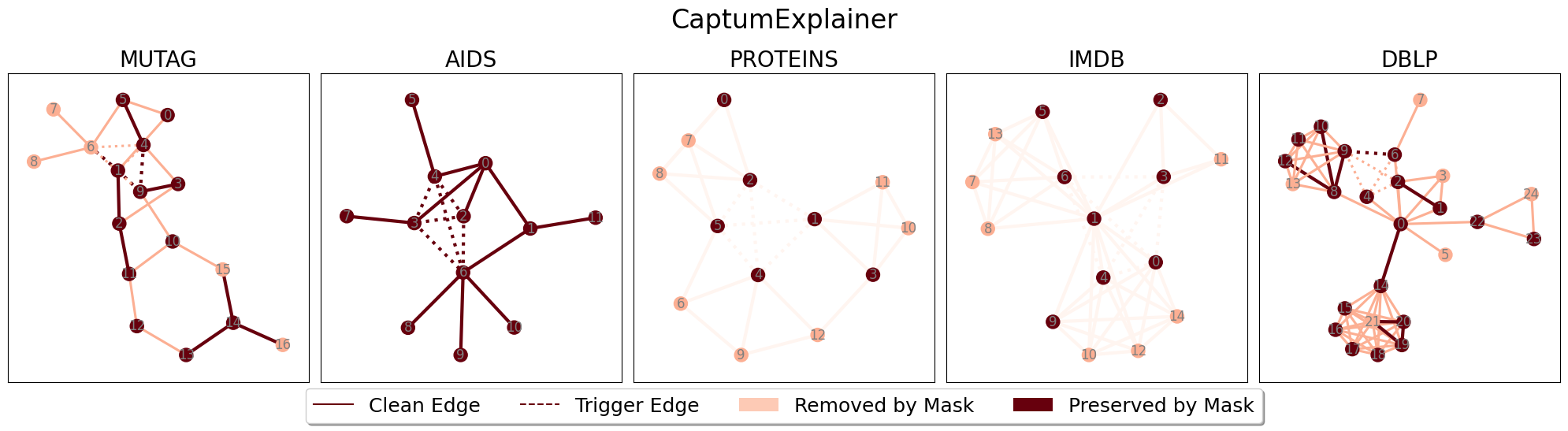
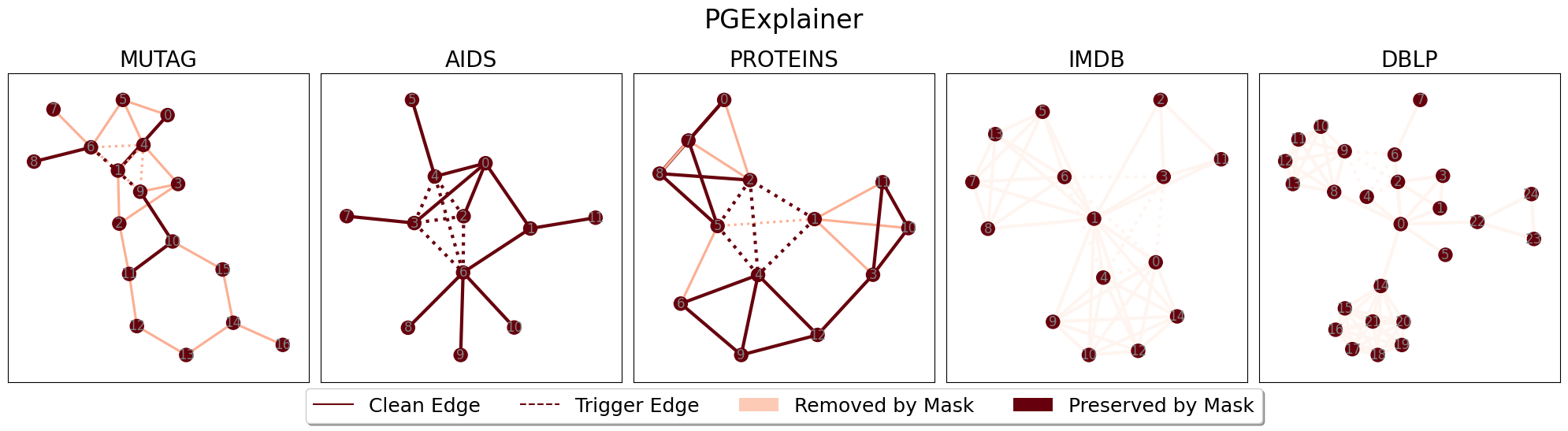
Figure S1: An example of a backdoored sample from each dataset, after applying the mask generated by CaptumExplainer (top) and PGExplainer (bottom). These explanations were generated using the same hyperparameters as in Figure 2.

Figure S1 illustrates the features preserved by CaptumExplainer and PGExplainer on our inputs. A comparison of these figures to Figure 2 illustrates a common theme – that explainer methods generally fail as a method for reverse engineering the trigger. In the MUTAG example, there is no obvious pattern to the way CaptumExplainer preserves or excludes either trigger or clean features, whereas in the AIDS example, all features are preserved. For PROTEINS and IMDB, trigger nodes are preserved, helping somewhat to identify the trigger, but all edges are excluded. And in the DBLP example, trigger nodes are preserved at a higher rate than clean nodes (4/4 versus 15/21), but only a few edges are preserved, and none of them belong to the trigger. Turning to PGExplainer results, we see similarly dissatisfying results – in no case does the explanatory subgraph exclusively preserve the triggered features. These failures across different explainers underscore the constraints of depending exclusively on explanatory subgraphs for the detection of backdoored instances.

Appendix 0.B GNNExplainer Settings and Fidelity

0.B.1 Phenomenon and Model Explanations

The GNNExplainer can compute two types of explanations: model explanations and phenomenon explanations.

• Model explanation: an explanation of the model’s actual prediction, revealing the logic that the model is most inclined to follow.

• Phenomenon explanation: an explanation of the model’s decision process for a user-specified outcome, revealing the parts of the input that are essential for predicting a particular target label.

We used phenomenon explanations of our experiments, instructing GNNExplainer to provide explanations of the ground truth label for each graph. Note that, in the case that the model is 100% accurate, a model explanation would produce identical results. However, in any other scenario, model explanations and phenomenon explanations have the potential to yield vastly different results. It is therefore crucial to be conscious of this setting when implementing our method.

0.B.2 Fidelity Variants

For phenomenon explanations, fidelity scores are defined as:

$$\text{fid}_{+}=|\mathbbm{1}(\hat{y}=y)-\mathbbm{1}(\hat{y}_{i}^{C}=y)|$$ (12)

$$\text{fid}_{-}=|\mathbbm{1}(\hat{y}=y)-\mathbbm{1}(\hat{y}^{S}=y)|$$ (13)

For model explanations, fidelity scores are defined as:

$$\text{fid}_{+}=1-\frac{1}{N}\sum_{i=1}^{N}\mathbbm{1}(\hat{y}_{i}^{G_{C}}=\hat{y}_{i})$$ (14)

$$\text{fid}_{-}=1-\frac{1}{N}\sum_{i=1}^{N}\mathbbm{1}(\hat{y}_{i}^{G_{S}}=\hat{y}_{i})$$ (15)

Recall that positive and negative fidelity are central to the computation of explainability (see Equation 3). Since these definitions are determined by the explanation type, this further emphasizes the importance of exercising caution in the choice between model and phenomenon explainer methods in the context of our backdoor detection method.

Appendix 0.C Metrics

0.C.1 Additional Detection Metric Distributions

In line with our earlier findings showcased in Figure 3, we now delve deeper into the detection metric distributions, this time focusing on two distinct scenarios: the injection of Preferential Attachment triggers of size 10 into 20% of the AIDS training data and an injection of Small World triggers of size 12 into 20% of the PROTEINS training data. In both cases, the target label is deliberately set to 1. To evaluate the impact of these attacks, we train a GIN classification model [43] on the poisoned AIDS dataset and a GAT classification model [36] on the poisoned PROTEINS dataset. Following the same setting mentioned in 5.1, we employ the GNNExplainer technique, utilizing a combination of clean validation data ($\mathcal{D}^{val}$) and a subset of the training data ($\mathcal{D}^{tr}$) that includes both clean and backdoored samples. This process results in the distributions depicted in Figure S2. The displayed distributions represent 110 graphs from each dataset, comprising 50 clean validation samples, 30 clean training samples, and 30 backdoored training samples.

These newly unveiled distributions underscore the diverse effectiveness of individual metrics, both within a dataset and across different types of metrics. Comparing these findings with those from Figure 3, we make several noteworthy observations. In Figure S2, metrics such as NDV and Prediction Confidence emerge as standout performers, demonstrating their considerable separation capability in these specific attack configurations. This suggests their pivotal role in effectively detecting and mitigating backdoor attacks under these circumstances. However, the story is nuanced, as Explainability exhibits reduced efficacy for both AIDS and PROTEINS, while Connectivity fails to perform optimally in the context of PROTEINS. These observations starkly contrast with their significance in the context of Figure 3. This divergence in metric effectiveness highlights the need for a holistic approach, emphasizing the importance of considering all available metrics to achieve robust detection and defense against backdoor attacks across diverse settings.

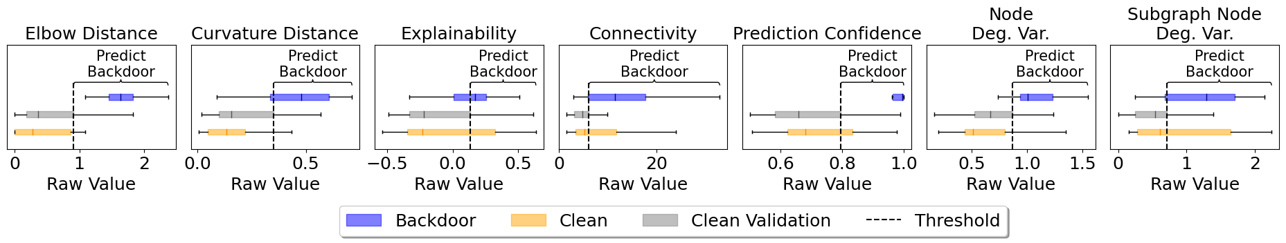
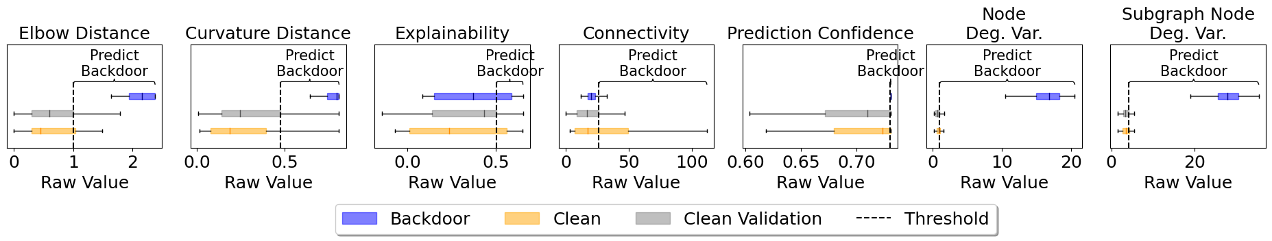
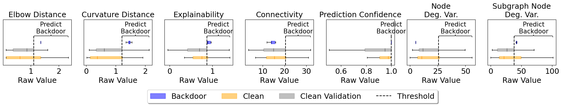
AIDS: Preferential Attachment Trigger (Size 10) PROTEINS: Small World Trigger (Size 12) IMDB-BINARY: Erdős-Rényi Trigger (Size 26) DBLP: Erdős-Rényi Trigger (Size 12)

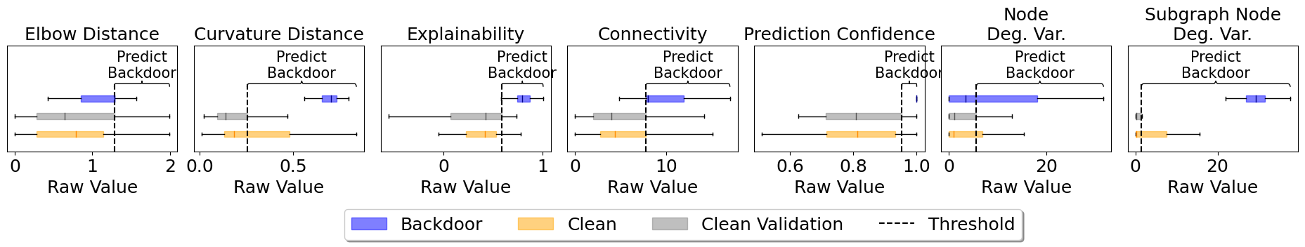
Figure S2: Additional examples of metric score distributions. Each set of distributions includes results from 50 clean validation samples, 30 clean training samples, and 30 backdoor samples. The AIDS distributions result from applying a Preferential Attachment trigger of size 10 to the training data and changing the labels of the corresponding graphs to 1. The PROTEINS distributions result from a similar process, except using a Small World trigger of size 12. For IMDB-BINARY, results are from an Erdős-Rényi trigger of size 26, and for DBLP, the results correspond to an Erdős-Rényi trigger of size 1. Taken in conjunction with Figure 3, these distributions underscore the diverse performance of individual metrics – including both the potential of each metric under varying circumstances and the risks of depending on any one metric in isolation.

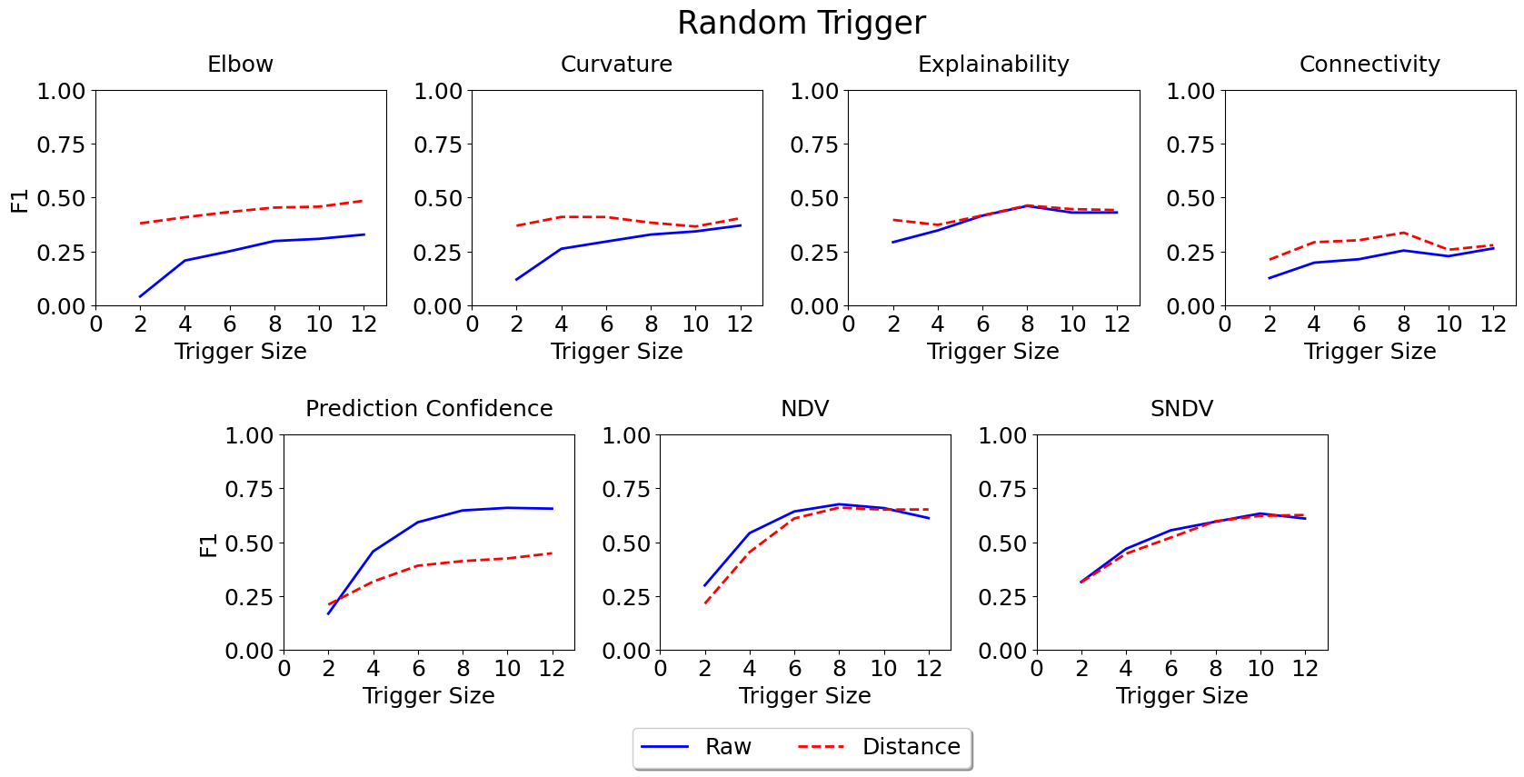
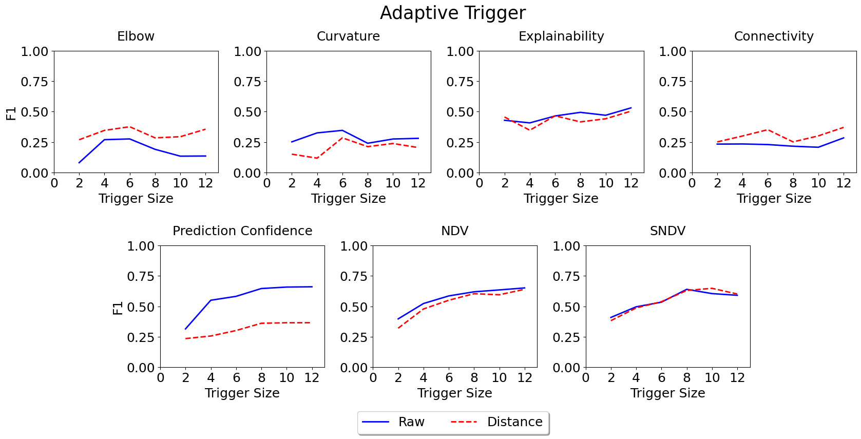
Figure S3: These figures compare raw and distance metrics across trigger sizes. The upper seven figures show results for attacks with random triggers, while the lower seven figures show results for attacks with adaptive triggers. For random triggers, Curvature and Elbow distance metrics tend to outperform their raw counterparts. This is particularly true for smaller triggers, which are harder to detect, leading the explainer loss curve to converge in accordance with the clean figures, which may be more recognizable. Conversely, in the case of Curvature, this caveat is no longer relevant when we consider adaptive attacks, likely because the adaptive triggers are stronger – even at small sizes – than their random counterparts.

0.C.2 Raw versus Distance Metrics

Figure S3 compares the relationships between raw data and various distance metrics across different trigger sizes. The insights gleaned from these comparisons shed light on the effectiveness of selecting distance-based metrics for Curvature and Elbow in contrast to their raw data counterparts. In the case of a random trigger, these two distance metrics consistently outperform their raw data counterparts, particularly when dealing with smaller trigger sizes. This phenomenon can be attributed to the inherent challenge of detecting smaller triggers, which often necessitates a more refined and sensitive approach. The rationale behind this trend lies in the behavior of the explainer loss curve. As trigger sizes decrease, the explainer loss curve tends to converge, aligning closely with the clean data figures. This convergence is due to the fact that smaller triggers are inherently harder to discern within the data. Consequently, GNNExplainer’s task becomes one of fitting the model to the clean data rather than detecting the subtle trigger presence.

For adaptive triggers, the superiority of distance metrics over raw metrics holds for Elbow, but not Curvature. Remember from section 4.2 that better performance from distance metrics over raw metrics corresponded to a reversal of our expectations for the metrics, indicating that explanations of backdoor samples were more in line with our expectations of clean samples. And as mentioned above, this is more likely to be the case in instances of a weak attack, which GNNExplainer would have a more difficult time discerning from clean instances. However, adaptive triggers produce stronger attacks than their random counterparts, even at smaller trigger sizes. In this case, the explainer loss curve will be more markedly different for backdoored samples than for clean samples, explaining why Curvature – a metric derived from the loss curve – is no longer subject to the reversed expectations that we witness with random attacks. This helps explain why the distance form of the Curvature metric is necessary in the case of random attacks, but not in adaptive attacks, where the raw form of the metric is sufficient.

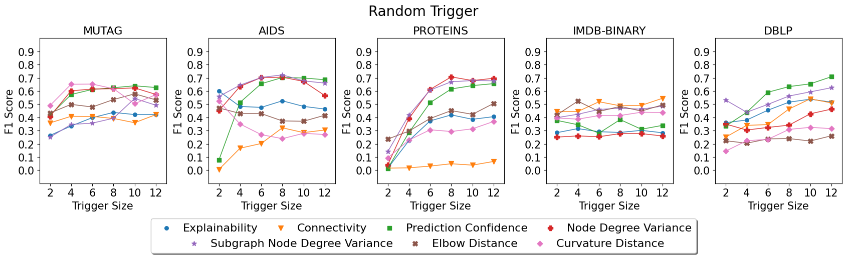
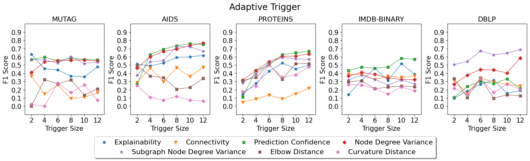
Figure S4: F1 score of each metric across varied trigger sizes, separated for attacks with random triggers (top) and adaptive triggers (bottom). For enhanced thoroughness, the random and adaptive figures incorporate results from 953 and 128 attack configurations, respectively. The diversity of performance across individual metrics across all configurations validates the need to use metrics collectively rather than individually.

0.C.3 Individual Metrics vs. Attack Strength

Figure S4 illustrates the effectiveness of each individual metric in the context of varied trigger sizes and datasets, in both random and adaptive attacks. There is widespread diversity in the effectiveness under the various settings. Considering the top row (corresponding to random triggers) in isolation, a comparison of all ten subfigures underscores the observations from Figure S2 that the performances of individual metrics vary significantly between datasets. A brief glance at the bottom row (adaptive triggers) yields the same conclusion.

Most subfigures highlight the impact of trigger size and attack strength on the resulting capabilities of each metric. In most instances, for most metrics, performance improves as trigger size increases, which is consistent with the findings from Figure 6 that trigger size is positively correlated with the composite metric score.

However, this is not uniformly the case, most notably for the results from adaptive triggers in the MUTAG dataset (the bottom left subfigure). This particular instance is likely due to the smaller number of observations from adaptive attacks (128 adaptive trigger configurations versus 953 random trigger configurations), which – especially in the context of a small dataset comprised of smaller graphs, such as MUTAG – may require further results to parse out steadier trends in individual metric behavior. However, even in instances where results were plentiful (i.e., results from random triggers), performance among metrics varied – consider Connectivity, which performs worst among all seven metrics on PROTEINS, but best for IMDB-BINARY.

Once again, the diversity of metric performance emphasizes the need to consider our metrics collectively.

Appendix 0.D Datasets

We used five datasets in our analysis – MUTAG [6], AIDS [30], PROTEINS [2], IMDB-BINARY [44], and DBLP [34]. Details can be viewed in Table 0.D. The inclusion of five datasets from different domains increases the variety of settings under which we could test our method. Our datasets included graphs ranging between 10 and 20 nodes, on average, and 16 and 97 edges, on average.

Table S1: Dataset Properties

Dataset	Num.
	Graph
	Avg.
	Avg.
	Edges
MUTAG	2	188	17.93	19.79
AIDS	2	2000	15.69	16.20
PROTEINS	2	1113	39.06	72.82
DBLP	2	5000	10.48	19.65
IMDB-BINARY	2	1000	19.77	96.53

1 Input: Untrained graph classifier ${f_{s}}^{0}$, untrained trigger edge generator $f_{gen}$, clean graph dataset $D$, a set of to-be-backdoored graphs $D_{B}\subset D$, with the target label $\hat{y}$, number of steps $T$, number of epochs #Epochs, GNNExplainer learning rate $\eta_{exp}$, edge generator learning rate $\eta_{gen}$, trigger size $s$

2 Output: Trained edge generator $f_{gen}$

3 $f_{gen}$ $\leftarrow$ ${f_{gen}}^{0}$;

4 $f_{s}$ $\leftarrow$ Train(${f_{s}}^{0}$, D);

5 while not converged do

6       for epoch=1 to #Epoch do

7             for $G=(\textbf{A},\textbf{X})$ in $D_{B}$ do

                   $\textbf{B}\leftarrow\textbf{11}^{\textrm{T}}-\textbf{I}-$A;

                    // B includes all non-existent edges

                   $(u,v)\leftarrow\text{argmax}_{u,v}$$f_{gen}$$($A$,\textbf{X},\textbf{B})$; // Find non-existing edge w.r.t. the maximum $f_{gen}$ output

                   $\hat{\textbf{A}}={\bf A}$, ${\bf\hat{A}}_{u,v}=1$ ;

                    // Add an edge $(u,v)$ to ${\bf\hat{A}}$

8                   $\textbf{M}^{\hat{\textbf{A}}}_{0}\leftarrow\text{Randomly initialize the mask on }\hat{\textbf{A}}$;

9                   for $t=0$ to $T$ do

10                         $L_{CE}\leftarrow\textsc{CrossEntropyLoss}($$f_{s}$$(\hat{\textbf{A}}\odot\textbf{M}^{\hat{\textbf{A}}}_{t},\textbf{X}),\hat{y})$;

11                         $\textbf{M}^{\hat{\textbf{A}}}_{t+1}\leftarrow\textbf{M}^{\hat{\textbf{A}}}_{t}-\eta_{exp}\frac{\partial{L_{CE}}}{\partial\textbf{M}^{\hat{\textbf{A}}}_{t}}$;

12                   end for

13                  $L_{gen}\leftarrow L_{gen}+\sum_{i,j}(\textbf{M}^{\hat{\textbf{A}}}_{T}\odot\textbf{B})_{ij}$;

14             end for

            $\theta_{gen}\leftarrow\theta_{gen}-\eta_{gen}\frac{\partial L_{gen}}{\partial{\theta_{gen}}}$ ;

              // Update $f_{gen}$ parameters

15            

16       end for

      $\hat{D}_{B}\leftarrow\textsc{Poison}(D_{B},f_{gen},s)$ ;

        // Call $f_{gen}$ for $s$ times on $D_{B}$ to generate backdoored graphs $\hat{D}_{B}$

       $f_{s}\leftarrow\textsc{Train}({f_{s}}^{0},{D}\setminus D_{B}\cup\hat{D}_{B})$ ;

        // Train $f_{s}$ on clean, backdoored graphs

17      

18 end while

Algorithm 1 Training an Adaptive Trigger Generator

Appendix 0.E Adaptive Attack

Remember that our backdoor detector is based on a designed combined metric that directly uses the information from GNN explanation process. Hence, the main idea of the proposed adaptive attack is to attack the GNN explainer: we learn a trigger generator that takes a graph and its non-existing edges as input and outputs a matrix of “scores” corresponding to each non-existing edge. As the generator trains, this “score” represents how effectively a new edge will evade explanation by a GNN explainer. In the end, the trigger generator can generate edges which are least likely included in the explanatory subgraph originally outputted by a GNN explainer.

0.E.1 Trigger Generation

The pseudocode in Algorithm 1 expands upon the process briefly outlined in section 4.4.

Attackers begin with an untrained GNN trigger edge generator, ${f_{gen}}^{0}$(line 3), and an untrained GNN graph classifier, ${f_{s}}^{0}$. In the first stage (line 4), they train ${f_{s}}^{0}$ on clean data to obtain $f_{s}$, and in each subsequent stage (line 22) they retrain ${f_{s}}^{0}$  from scratch, on a dataset attacked with the most recent iteration of the trigger generator.

Edge generator $f_{gen}$ trains iteratively, in multiple rounds, over a subset of clean graphs $D$ designated for attack (denoted as $D_{B}$) (line 8-line 19). Each graph $G=({\bf A},{\bf X})\in D_{B}$ is fed to $f_{gen}$  which outputs a score for each (not-yet-existing) edge in B. As $f_{gen}$ trains, learning to evade GNNExplainer, these scores will correspond to the likelihood of an edge being excluded by GNNExplainer – i.e., the stealthiness of each edge choice. Therefore, the edge with the highest score is the one marked for inclusion in the trigger (line 10). The matrix $\hat{\textbf{A}}$ equals the raw adjacency matrix A modified to include this added edge (line 11).

After obtaining $\hat{\textbf{A}}$, attackers simulate GNNExplainer’s iterative process (over $T$ steps) of selecting an optimal explanatory mask, $\textbf{M}^{\hat{\textbf{A}}}_{t}$. This is where $f_{s}$ comes in – in each mask optimization step $t$, the attackers compute cross-entropy loss on $f_{s}$’s prediction on a graph with edges weighted by $\textbf{M}^{\hat{\textbf{A}}}_{t}$; they then update $\textbf{M}^{\hat{\textbf{A}}}_{t}$ in the opposite direction of the gradient with respect to $\textbf{M}^{\hat{\textbf{A}}}_{t}$ (line 15).

At the end of processing each graph, the final step is to update the running loss value, $L_{gen}$ (line 17). The objective function (Equation 11) aims to find the $f_{gen}$ whose edge predictions evade explanation by GNNExplainer. Therefore, the loss associated with each graph equals the summed explanation mask values associated with the newest edges. By masking $\textbf{M}^{\hat{\textbf{A}}}_{t}$ by B within this summation, attackers limit the influence on this loss term to non-clean edges only.

After iterating over all to-be-backdoored graphs $D_{B}$, edge generator parameters $\theta_{gen}$ are updated in the opposite direction of the gradient (line 20). To obtain a poisoned dataset $\hat{\textit{D}}$, for each graph in $D_{B}$ designated for backdoor, attackers call $f_{gen}$ for $s$ times in order to inject a trigger with $s$ edges. They then train (from scratch) a new classifier $f_{s}$ on the results. By retraining the model $f_{s}$ on this attacked dataset between iterations, attackers simulate a more realistic scenario, in which GNNExplainer would be operating against an already-attacked GNN.

The above process is repeated until $L_{gen}$ converges. In the end, attackers have a fully-trained edge generator $f_{gen}$, which can generate triggers of arbitrary size (one edge at a time). The attackers then use this generator $f_{gen}$ to generate adaptive triggers within a dataset marked for attack.

0.E.2 Trigger Generator Settings

In our experiments, $f_{gen}$ is a neural network with 4 fully-connected layers; The architecture of this trigger generator $f_{gen}$ is as follows:

• Linear(number of node features, 64), ReLU

• Linear(64, 64), Batchnorm, ReLU

• Linear(64, 64), Batchnorm, ReLU

• Linear(64, 1)

The hyperparameters of the trigger generators were tweaked according to the needs of each dataset. In general, these values are as follows:

• $\eta_{exp}$: 0.005 to 0.05

• $\eta_{gen}$: 0.005 to 0.05

• #Epoch: 20

• T: 50 to 100

Appendix 0.F Computational Complexity

The proposed backdoor detection method is dominated by the explanation method. Our method consists of 1) running a GNN explainer and 2) computing a composite of 7 metrics using results of the explanation process. The computational complexity of 2) is computed in constant time, and is negligible compared with 1). Therefore, the computational complexity of our method is determined by the explainer algorithm selected.

References

- [1] Barabási, A.L., Albert, R.: Emergence of scaling in random networks. science (1999)
- [2] Borgwardt, K.M., Ong, C.S., Schönauer, S., Vishwanathan, S.V.N., Smola, A.J., Kriegel, H.P.: Protein function prediction via graph kernels. Bioinformatics 21 (06 2005). https://doi.org/10.1093/bioinformatics/bti1007, https://doi.org/10.1093/bioinformatics/bti1007
- [3] Chen, K., Meng, Y., Sun, X., Guo, S., Zhang, T., Li, J., Fan, C.: Badpre: Task-agnostic backdoor attacks to pre-trained nlp foundation models. In: International Conference on Learning Representations (2022)
- [4] Chen, X., Liu, C., Li, B., Lu, K., Song, D.: Targeted backdoor attacks on deep learning systems using data poisoning. arXiv (2017)
- [5] Clements, J., Lao, Y.: Hardware trojan attacks on neural networks. arXiv preprint arXiv:1806.05768 (2018)
- [6] Debnath, A.K., Lopez de Compadre, R.L., Debnath, G., Shusterman, A.J., Hansch, C.: Structure-activity relationship of mutagenic aromatic and heteroaromatic nitro compounds. correlation with molecular orbital energies and hydrophobicity. Journal of medicinal chemistry (1991)
- [7] Gan, L., Li, J., Zhang, T., Li, X., Meng, Y., Wu, F., Yang, Y., Guo, S., Fan, C.: Triggerless backdoor attack for nlp tasks with clean labels. In: Proceedings of the 2022 Conference of the North American Chapter of the Association for Computational Linguistics: Human Language Technologies. pp. 2942–2952 (2022)
- [8] Gao, Y., Xu, C., Wang, D., Chen, S., Ranasinghe, D.C., Nepal, S.: Strip: A defence against trojan attacks on deep neural networks. In: ACSAC (2019)
- [9] Ge, Y., Wang, Q., Yu, J., Shen, C., Li, Q.: Data poisoning and backdoor attacks on audio intelligence systems. IEEE Communications Magazine (2023)
- [10] Gilbert, E.N.: Random graphs. Ann. Math. Stat. (1959)
- [11] Gu, T., Dolan-Gavitt, B., Garg, S.: Badnets: Identifying vulnerabilities in the machine learning model supply chain. In: Proc. of Machine Learning and Computer Security Workshop (2017)
- [12] Guan, Z., Du, M., Liu, N.: Xgbd: Explanation-guided graph backdoor detection. arXiv preprint arXiv:2308.04406 (2023)
- [13] Guo, H., Chen, X., Guo, J., Xiao, L., Yan, Q.: Masterkey: Practical backdoor attack against speaker verification systems. In: Proceedings of the 29th Annual International Conference on Mobile Computing and Networking. pp. 1–15 (2023)
- [14] Guo, W., Wang, L., Xing, X., Du, M., Song, D.: Tabor: A highly accurate approach to inspecting and restoring trojan backdoors in ai systems. arXiv preprint arXiv:1908.01763 (2019)
- [15] Hamilton, W., Ying, Z., Leskovec, J.: Inductive representation learning on large graphs. In: NeurIPS (2017)
- [16] Hassen, M., Chan, P.K.: Scalable function call graph-based malware classification. In: CODASPY (2017)
- [17] Jiang, B., Li, Z.: Defending against backdoor attack on graph neural network by explainability. arXiv preprint arXiv:2209.02902 (2022)
- [18] Kipf, T.N., Welling, M.: Semi-supervised classification with graph convolutional networks. In: ICLR (2017)
- [19] Kokhlikyan, N., Miglani, V., Martin, M., Wang, E., Alsallakh, B., Reynolds, J., Melnikov, A., Kliushkina, N., Araya, C., Yan, S., Reblitz-Richardson, O.: Captum: A unified and generic model interpretability library for pytorch (2020)
- [20] Li, W., Yu, J., Ning, X., Wang, P., Wei, Q., Wang, Y., Yang, H.: Hu-fu: Hardware and software collaborative attack framework against neural networks. In: ISVLSI. IEEE (2018)
- [21] Liu, K., Dolan-Gavitt, B., Garg, S.: Fine-pruning: Defending against backdooring attacks on deep neural networks. In: RAID (2018)
- [22] Liu, Y., Lee, W.C., Tao, G., Ma, S., Aafer, Y., Zhang, X.: Abs: Scanning neural networks for back-doors by artificial brain stimulation. In: SIGSAC (2019)
- [23] Liu, Y., Ma, S., Aafer, Y., Lee, W.C., Zhai, J., Wang, W., Zhang, X.: Trojaning attack on neural networks. In: NDSS (2018)
- [24] Liu, Y., Xie, Y., Srivastava, A.: Neural trojans. In: 2017 IEEE International Conference on Computer Design (ICCD). IEEE (2017)
- [25] Luo, D., Cheng, W., Xu, D., Yu, W., Zong, B., Chen, H., Zhang, X.: Parameterized explainer for graph neural network. Advances in neural information processing systems 33, 19620–19631 (2020)
- [26] Pal, S., Wang, R., Yao, Y., Liu, S.: Towards understanding how self-training tolerates data backdoor poisoning. arXiv preprint arXiv:2301.08751 (2023)
- [27] Pan, X., Zhang, M., Sheng, B., Zhu, J., Yang, M.: Hidden trigger backdoor attack on NLP models via linguistic style manipulation. In: 31st USENIX Security Symposium (USENIX Security 22). pp. 3611–3628 (2022)
- [28] Pope, P.E., Kolouri, S., Rostami, M., Martin, C.E., Hoffmann, H.: Explainability methods for graph convolutional neural networks. In: Proceedings of the IEEE/CVF conference on computer vision and pattern recognition. pp. 10772–10781 (2019)
- [29] Qi, F., Li, M., Chen, Y., Zhang, Z., Liu, Z., Wang, Y., Sun, M.: Hidden killer: Invisible textual backdoor attacks with syntactic trigger. In: Proceedings of the 59th Annual Meeting of the Association for Computational Linguistics and the 11th International Joint Conference on Natural Language Processing (Volume 1: Long Papers). pp. 443–453 (2021)
- [30] Riesen, K., Bunke, H.: Iam graph database repository for graph based pattern recognition and machine learning. In: Da Vitora Lobo, N. et al. (Eds.), SSPR/SPR 2008 pp. 287–297 (2008)
- [31] Roy, N., Hassanieh, H., Roy Choudhury, R.: Backdoor: Making microphones hear inaudible sounds. In: Proceedings of the 15th Annual International Conference on Mobile Systems, Applications, and Services. pp. 2–14 (2017)
- [32] Salem, A., Wen, R., Backes, M., Ma, S., Zhang, Y.: Dynamic backdoor attacks against machine learning models. In: EuroSP (2022)
- [33] Shi, C., Zhang, T., Li, Z., Phan, H., Zhao, T., Wang, Y., Liu, J., Yuan, B., Chen, Y.: Audio-domain position-independent backdoor attack via unnoticeable triggers. In: Proceedings of the 28th Annual International Conference on Mobile Computing And Networking. pp. 583–595 (2022)
- [34] Tang, J., Zhang, J., Yao, L., Li, J., Zhang, L., Su, Z.: Arnetminer: extraction and mining of academic social networks. In: Proceedings of the 14th ACM SIGKDD International Conference on Knowledge Discovery and Data Mining. p. 990–998. KDD ’08, Association for Computing Machinery, New York, NY, USA (2008). https://doi.org/10.1145/1401890.1402008, https://doi.org/10.1145/1401890.1402008
- [35] Tran, B., Li, J., Madry, A.: Spectral signatures in backdoor attacks. In: NeurIPS (2018)
- [36] Veličković, P., Cucurull, G., Casanova, A., Romero, A., Lio, P., Bengio, Y.: Graph attention networks. In: ICLR (2018)
- [37] Wang, B., Cao, X., Jia, J., Gong, N.Z.: On certifying robustness against backdoor attacks via randomized smoothing. In: CVPR Workshop (2020)
- [38] Wang, B., Yao, Y., Shan, S., Li, H., Viswanath, B., Zheng, H., Zhao, B.Y.: Neural cleanse: Identifying and mitigating backdoor attacks in neural networks. In: IEEE S&P (2019)
- [39] Wang, R., Zhang, G., Liu, S., Chen, P.Y., Xiong, J., Wang, M.: Practical detection of trojan neural networks: Data-limited and data-free cases. In: Computer Vision–ECCV 2020: 16th European Conference, Glasgow, UK, August 23–28, 2020, Proceedings, Part XXIII 16. pp. 222–238. Springer (2020)
- [40] Watts, D.J., Strogatz, S.H.: Collective dynamics of ‘small-world’networks. nature (1998)
- [41] Weber, M., Xu, X., Karlaš, B., Zhang, C., Li, B.: Rab: Provable robustness against backdoor attacks. In: 2023 IEEE Symposium on Security and Privacy (SP). pp. 1311–1328. IEEE (2023)
- [42] Xi, Z., Pang, R., Ji, S., Wang, T.: Graph backdoor. In: 30th USENIX Security Symposium (USENIX Security 21). pp. 1523–1540 (2021)
- [43] Xu, K., Hu, W., Leskovec, J., Jegelka, S.: How powerful are graph neural networks? In: International Conference on Learning Representations (2019)
- [44] Yanardag, P., Vishwanathan, S.: Deep graph kernels. In: Proceedings of the 21th ACM SIGKDD International Conference on Knowledge Discovery and Data Mining. p. 1365–1374. KDD ’15, Association for Computing Machinery, New York, NY, USA (2015). https://doi.org/10.1145/2783258.2783417, https://doi.org/10.1145/2783258.2783417
- [45] Yao, Y., Li, H., Zheng, H., Zhao, B.Y.: Latent backdoor attacks on deep neural networks. In: CCS (2019)
- [46] Ying, R., Bourgeois, D., You, J., Zitnik, M., Leskovec, J.: Gnnexplainer: Generating explanations for graph neural networks. In: Advances in Neural Information Processing Systems 32 (2019)
- [47] Zhang, X.M., Liang, L., Liu, L., Tang, M.J.: Graph neural networks and their current applications in bioinformatics. Frontiers in Genetics 12 (2021). https://doi.org/10.3389/fgene.2021.690049, https://www.frontiersin.org/articles/10.3389/fgene.2021.690049
- [48] Zhang, Z., Jia, J., Wang, B., Gong, N.Z.: Backdoor attacks to graph neural networks. In: Proceedings of the 26th ACM Symposium on Access Control Models and Technologies. pp. 15–26 (2021)
- [49] Zhao, S., Ma, X., Zheng, X., Bailey, J., Chen, J., Jiang, Y.G.: Clean-label backdoor attacks on video recognition models. In: Proceedings of the IEEE/CVF conference on computer vision and pattern recognition. pp. 14443–14452 (2020)
- [50] Zhou, J., Cui, G., Hu, S., Zhang, Z., Yang, C., Liu, Z., Wang, L., Li, C., Sun, M.: Graph neural networks: A review of methods and applications. AI Open 1, 57–81 (2020). https://doi.org/https://doi.org/10.1016/j.aiopen.2021.01.001, https://www.sciencedirect.com/science/article/pii/S2666651021000012