Revisiting Elastic String Models of Forward Interest Rates

Abstract

Twenty five years ago, several authors proposed to model the forward interest rate curve (FRC) as an elastic string along which idiosyncratic shocks propagate, accounting for the peculiar structure of the return correlation across different maturities. In this paper, we revisit the specific “stiff” elastic string field theory of Baaquie and Bouchaud [1] in a way that makes its micro-foundation more transparent. Our model can be interpreted as capturing the effect of market forces that set the rates of nearby tenors in a self-referential fashion. The model is parsimonious and accurately reproduces the whole correlation structure of the FRC over the time period $1994-2023$, with an error below $2\%$. We need only two parameters, the values of which being very stable except perhaps during the Quantitative Easing period $2009-2014$. The dependence of correlation on time resolution (also called the Epps effect) is also faithfully reproduced within the model and leads to a cross-tenor information propagation time of $\approx 10$ minutes. Finally, we confirm that the perceived time in interest rate markets is a strongly sub-linear function of real time, as surmised by Baaquie and Bouchaud [1]. In fact, our results are fully compatible with hyperbolic discounting, in line with the recent behavioural literature [2].

I Introduction

I.1 Motivation

The forward interest rate $f(t,T)$, to be defined more precisely below, is the interest rate agreed upon at time $t$, for an instantaneous loan between $T\geq t$ and $T+dT$. Such a collection of future rates defines a kind of “string” that moves and deforms with time. Understanding the dynamics of the forward interest rate curve (FRC) is crucial in a wide spectrum of financial applications, ranging from the valuation of interest rate derivatives to risk management [3, 4]. This problem is also fascinating from a theoretical point of view: whereas the stochastic process governing the dynamics of single assets (point-like objects) has been heavily documented [5, 6, 7, 8, 9, 10, 11, 12, 13], the stochastic process of higher dimensional objects like lines or graphs is much more involved. There is a long tradition in the physics literature of modelling string-like (or surface-like) objects which has not yet pervaded into the financial mathematics literature, despite early attempts [14, 15, 1].

The aim of this paper is to revisit the 2004 proposal of Belal Baaquie and one of the author (JPB), to describe the returns of different tenors of the FRC in terms of the fluctuations of a “stiff” elastic string – called henceforth the BB04 model [1]. We will see that up to a redefinition of their model that accounts for the discrete set of maturities defining the FRC (instead of the continuum limit of BB04), the proposed framework allows one to account quite remarkably for the full cross-maturity correlation structure of the FRC, across the whole period 1994-2023 (when the BB04 model was only tested for the period 1994-1996).

I.2 Definitions and notations

We recall here the definition of the risk-free instantaneous forward interest rate. Table 1 in appendix A provides the complete list of the notations used in this study.

Zero-coupon Bond.

Let $P(t,T)$ represent the price at time $t$ of a zero-coupon bond maturing at $T$. Such a bond pays one unit of currency at maturity $T$ without any intermediate coupons.

Forward Rate.

Consider time $t$ and two future times, $S$ and $T$, where $t<S<T$. The forward rate, a risk-free interest rate for the period $[S,T]$, is derived from zero-coupon bonds. By selling a zero-coupon bond maturing at $S$ for $P(t,S)$ euros and purchasing $\frac{P(t,S)}{P(t,T)}$ units of a bond maturing at $T$, we establish a contract that costs nothing at $t$, pays one unit of currency at $S$, and yields $\frac{P(t,S)}{P(t,T)}$ euros at $T$. This setup leads to a deterministic rate of return, with the continuously compounded forward rate $R(t,S,T)$ given by:

$$e^{R(t,S,T)(T-S)}=\frac{P(t,S)}{P(t,T)},$$ (1)

solving to:

$$R(t,S,T)=-\frac{\log{P(t,T)}-\log{P(t,S)}}{T-S}.$$ (2)

Instantaneous Forward Rate.

As $S$ approaches $T$, the limit of $R(t,S,T)$ defines the instantaneous forward rate $f(t,T)$:

$$f(t,T)=-\frac{\partial\log{P(t,T)}}{\partial T},$$ (3)

The collection of these rates for various $T$ forms the forward rate curve (FRC).

In the following sections, we actually define the instantaneous forward rate $f(t,\theta)$ in terms of the time to maturity or tenor $\theta=T-t$. This dimension $\theta$ is often referred to as the space dimension, as opposed to the time dimension $t$.

I.3 The Heath-Jarrow-Morton framework

The Heath-Jarrow-Morton (HJM) framework has become the industry standard [16, 17]. Within this framework, the FRC dynamics is modeled using Itô processes driven by a $d$-dimensional Brownian motion. Consequently, bond prices for each tenor $\theta$ are regarded not as financial derivatives of the risk-free rate $f(t,0)$ but as individual risky assets, leading to an possibly infinite number of such assets. The finite number $d$ of diffusion factors introduces the potential for arbitrage opportunities among bond prices [18]. Thus, conditions are established on the drift components of instantaneous forward rate processes to ensure arbitrage-free pricing of zero-coupon bonds. This framework rests only on two fundamental assumptions: the continuity of sample paths for forward rate processes and a finite number of Brownian motions driving these processes.

Beyond the fact that the HJM model has no ambition to capture the “physical”, one dimensional nature of the FRC, a limitation of the HJM framework is its stipulation that for any integer $k$, the correlation matrix of $k+d$ instantaneous forward rates must be singular when the model employs $d$ factors. This condition is in conflict with empirical observations. Addressing this limitation, various researchers have ventured beyond the conventional boundary of a finite number of driving Brownian motions. Notably, Kennedy [19, 20] proposed to model each forward rate by a Gaussian random field while Cont [21], Goldstein [22] and Santa-Clara and Sornette [15] developed stochastic string approaches, partly based on the empirical work of [14] where the idea of the FRC as an elastic string was first put forth.

Among these advancements, Baaquie [23, 24, 25] has pioneered a quantum field theory approach, set to be further discussed in the ensuing section. In the following years, these random field theories have been applied to solve interest rate derivatives pricing problems [26, 27, 28, 29, 30, 31, 32, 33, 34, 35, 36].

II A field theory for the FRC

Baaquie [23, 24, 25] introduced a two-dimensional field theory to model the forward interest rate curve. This approach was generalized in BB04 Baaquie and Bouchaud [1] to account for the pronounced smoothness observed in the correlation matrix of forward rate increments. More precisely, it was observed in [14] that the eigenvectors of the covariance matrix of the FRC returns had the same structure as those of a elastic string and can be indexed by the number $n$ of zeroes in the $\theta$ direction. The corresponding eigenvalues were found to behave as $(a+bn^{2})^{-1}$ for small $n$ (where $a,b$ are constants), crossing over to a faster decay $\approx n^{-4}$ for larger $n$’s (see Fig. 5 of [14]).

A way to encode this empirical finding is to posit that the dynamics of the FRC $f(t,\theta)$ is specified by a drift velocity $\gamma(t,\theta)$ and a volatility $\sigma(t,\theta)$, such that:

$$\frac{\partial f}{\partial t}(t,\theta) =\gamma(t,\theta)+\sigma(t,\theta)A(t,\theta),$$ (4)

where $A(t,\theta)$ represents a driftless noise field.

The “field theory” formulation assumes that $\theta$ is a continuous variable $\in\mathbb{R}_{+}$ and the joint probability distribution across time and tenor for the set of noises $\left\{A(t,\theta)\right\}_{(t,\theta)\in\mathbb{R}_{+}^{2}}$ is determined by the exponential of an action $S[A]$. This action is a functional defined over the semi-infinite domain $\mathbb{R}_{+}^{2}$, and is given by:

$$S[A]:= -\frac{1}{2}\iint_{0}^{\infty}{\rm d}t{\rm d}\theta\,\Bigg{(}\Bigg{.}A^{2}(t,\theta)$$

$$+\left(\frac{1}{\mu}\frac{\partial A}{\partial\theta}(t,\theta)\right)^{2}+\left(\frac{1}{\nu^{2}}\frac{\partial^{2}A}{\partial\theta^{2}}(t,\theta)\right)^{2}\Bigg{.}\Bigg{)},$$ (5)

with $\mu^{-2}$ and $\nu^{-4}$ denoting respectively the “line tension” and “stiffness” (also called bending rigidity) parameters, which have the physical dimensions of frequencies. More precisely, small values of $\mu$ disfavor large local slopes of $A(t,\theta)$ whereas small values of $\nu$ disfavor large local curvatures.

A boundary condition is needed for the theory to be complete, and was postulated in [1] to be of the Neumann type, i.e.

$$\left.\frac{\partial A(t,\theta)}{\partial\theta}\right|_{T=t} =0,$$ (6)

thereby enforcing a uniform motion of the forward interest rates at very short maturities. This assumption is justified considering the spot rate $f(t,0)$ is typically set by the Central Bank, and very short-term maturities carry minimal additional risk.

Within this modeling framework, the noise correlator is defined as:

$$\langle A(t,\theta)A(t^{\prime},\theta^{\prime})\rangle =\delta(t-t^{\prime})\mathcal{D}_{BB}(\theta,\theta^{\prime}),$$ (7)

where the brackets denote an averaging over the functional weight $e^{S[A]}$, and where $\mathcal{D}_{BB}(\theta,\theta^{\prime})$ is found to be [1]

$$\mathcal{D}_{BB}(\theta,\theta^{\prime}) =\frac{\nu^{4}}{\alpha_{+}-\alpha_{-}}\left[\frac{F(\theta,\theta^{\prime},\sqrt{\alpha_{-}})}{\alpha_{-}}-\frac{F(\theta,\theta^{\prime},\sqrt{\alpha_{+}})}{\alpha_{+}}\right],$$ (8)

with

$$\alpha_{\pm}=\frac{\nu^{4}}{2\mu^{2}}\left[1\pm\sqrt{1-4\left(\frac{\mu}{\nu}\right)^{4}}\right]$$

and

$$F(\theta,\theta^{\prime},\kappa) :=\frac{\kappa}{2}\left(e^{-\kappa(\theta+\theta^{\prime})}+e^{-\kappa|\theta-\theta^{\prime}|}\right).$$ (9)

Formally, absence of arbitrage among zero-coupon bond prices imposes the following condition on the drift $\gamma(t,\theta)$ [25]:

$$\gamma(t,\theta) =\sigma(t,\theta)\int_{0}^{\theta}{\rm d}\theta^{\prime}\mathcal{D}_{BB}(\theta^{\prime})\sigma(t,\theta^{\prime}),$$ (10)

though this term is usually completely negligible numerically [14].

This theory further introduced the concept of psychological time which explains how the perceived time $\theta^{\prime}-\theta$ between tenors varies with their distance $\theta$ from the observer standing at time $t$, introducing one more parameter called ${\psi}$ below (see section IV.2 below). This framework allows one to fit the whole empirical correlation matrix $\rho_{\theta\theta^{\prime}}$ with only three meaningful parameters $\mu,\nu$ and ${\psi}$. Within this model, and in line with observations, the curvature of the forward rate correlation perpendicular to the diagonal, decays as power-law with respect to maturity (see Appendix F). This was perhaps the most salient success of the BB04 model, which however fell into almost complete oblivion (only 12 citations to date!).

In spite of its phenomenological success, the BB04 model has two main limitations.

1. First, the theory assumes a continuous spectrum of futures contracts across different tenors $\theta$, whereas in reality, futures contracts are available only at discrete tenors, usually every three calendar months. In other words, continuous derivatives like $\partial_{\theta}A$ have no physical existence.

2. Second, it predicts a constant correlation structure across all time scales used to define returns. This contradicts the well known “Epps effect”, i.e. the influence of the temporal granularity used to analyze prices [37, 38, 39]. Specifically, for the SOFR futures prices, Fig. 1 illustrates that the correlation between pairs of tenors ranging from 3 to 60 months emerges only after several minutes.

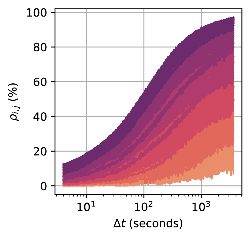
Figure 1: Pearson correlation coefficients $\rho(\theta,\theta^{\prime})$ as a function of the time scale $\Delta t$ used to define returns, for each pair of SOFR Futures prices of time-to-maturity $\theta$ ranging from $3$-month to $60$-month for the year $2021$. Each color correspond to a pair ordered from lowest (orange) to the hightest (purple) correlation level at the $1$-hour bin.

The aim of the present paper is to revisit the BB04 model with the two above deficiencies in mind. We reformulate the model in a way that makes its micro-foundations more apparent. We show in particular that market participants enforce a self-referential dynamics to the FRC, where each tenor is directly influenced by the motion of its neighbours. Furthermore, our dynamical formulation encapsulates market micro-structure phenomena, including the Epps effect, non-martingale prices at short scales and price-impact and cross-impact effects. The latter will be detailed in a companion paper Le Coz et al. [40].

III A Dynamical Reformulation

III.1 The continuous limit

We now want to interpret the above driftless noise field $A(t,\theta)$, as the solution to a differential equation that will generate temporal correlation over a time scale $\tau\ll 1$ day.

Consider $\eta(t,\theta)$ to be a two-dimensional white (Langevin) noise, characterized by the covariance function $\langle\eta(t,\theta)\eta(t^{\prime},\theta^{\prime})\rangle=2D\delta(t-t^{\prime})\delta(\theta-\theta^{\prime})$, where $\delta(\cdot)$ represents the Dirac delta function. We now write a stochastic equation for $A(t,\theta)$ such that its stationary measure is given by $e^{S[A]/D}$ (with $2D=1$ in the previous section):

$$\frac{\partial A}{\partial t}(t,\theta)=\frac{1}{\tau}\left(\frac{\delta S[A]}{\delta A(t,\theta)}+\eta(t,\theta)\right),$$ (11)

where $\tau$ is the characteristic time scale for the emergence of correlations. This equation, alongside the Neumann boundary condition specified in Eq. (6), can be expressed through the following linear differential equation:

$$\left\{\begin{aligned} &\frac{\partial A}{\partial t}(t,\theta)=\frac{1}{\tau}\left[-\mathcal{L}[A](t,\theta)+\eta(t,\theta)\right],\\ &\frac{\partial A}{\partial\theta}(t,0)=0,\end{aligned}\right.$$ (12)

where

$$\mathcal{L}[A](t,\theta):=A(t,\theta)-\frac{1}{\mu^{2}}\frac{\partial^{2}A}{\partial\theta^{2}}(t,\theta)+\frac{1}{\nu^{4}}\frac{\partial^{4}A}{\partial\theta^{4}}(t,\theta).$$

Eq. (12) describes how the correlated noise field $A(t,\theta)$ responds to the uncorrelated shocks $\eta(t,\theta)$, for example order flow at the microstructure level. However, as noted above, the above formulation presumes a continuous spectrum of tenors $\theta$, whereas, in practice, forward rates are observed at discrete maturities only. As will be shown below, this is not a trivial difference. In order to enhance the realism of our model, we now discretize the above equation with respect to $\theta$.

III.2 A discrete counterpart

In the following sections, we denote $x_{\theta}$ any variable defined on the discrete space of the tenors. Notably, $f(t,\theta)$ becomes $f_{\theta}(t)$ and $A(t,\theta)$ becomes $A_{\theta}(t)$. The discretization of Eq. (12) reads:

$$\left\{\begin{aligned} &\frac{{\rm d}A_{\theta}}{{\rm d}t}(t)=\frac{1}{\tau}\left[-\mathcal{L}_{d}[A]_{\theta}(t)+\eta_{\theta}(t)\right],\\ &A_{1}(t)-A_{0}(t)=0,\end{aligned}\right.$$ (13)

where the linear operator $\mathcal{L}$ have been substituted by its naive discrete counterpart $\mathcal{L}_{d}$:

$$\mathcal{L}_{d}[A]_{\theta}(t) :=A_{\theta}(t)-\frac{1}{\mu^{2}}\sum_{i=0}^{2}(-1)^{i}{\binom{2}{i}}A_{\theta+(1-i)}(t)$$ (14)

$$\quad+\frac{1}{\nu^{4}}\sum_{i=0}^{4}(-1)^{i}{\binom{4}{i}}A_{\theta+(2-i)}(t),$$

where $\theta$ is counted in multiple of 3 months and $\mu$ and $\nu$ are now dimension-less.

This discrete operator $\mathcal{L}_{d}$ mimics the impact of economic agents who compare the change of rate of a given tenor to the interpolation of the rates of its closest tenors. In fact, it seems intuitively plausible that agents primarily look at the two nearest tenors $\theta\pm 1$, corresponding to $1/\nu\to 0$. We will see below that the calibration of the model suggests that this is indeed the case.

The discretization of Eq. (12) also requires to replace the continuous noise $\eta(t,\theta)$ by a discrete Langevin noise $\eta_{\theta}(t)$, such that:

$$\langle\eta_{\theta}(t)\eta_{\theta^{\prime}}(t^{\prime})\rangle=2D\delta(t-t^{\prime})\delta_{\theta\theta^{\prime}},$$ (15)

where $\delta_{\theta\theta^{\prime}}$ is the Kronecker delta.

III.3 Building a correlated discrete random field

The solution to the discretized master Eq. (13) is given by

$$A_{\theta}(t)=\frac{1}{\tau}\int_{-\infty}^{t}{\rm d}t^{\prime}\sum_{\theta^{\prime}=0}^{+\infty}G_{\theta\theta^{\prime}}(t-t^{\prime})\eta_{\theta^{\prime}}(t^{\prime}),$$ (16)

where $G_{\theta\theta^{\prime}}(t-t^{\prime})$ is the propagator of the noise $\eta_{\theta^{\prime}}$ defined by

$$G_{\theta\theta^{\prime}}(t-t^{\prime}):=$$

$$\frac{1}{2\pi}\int_{-\pi}^{\pi}{\rm d}\xi\left(e^{i\xi(\theta-\theta^{\prime})}+e^{i\xi(\theta+\theta^{\prime})}\right)e^{-\frac{L_{d}(\xi)}{\tau}(t-t^{\prime})},$$ (17)

with $L_{d}(\xi)=1+2\frac{(1-\cos{\xi})}{\mu^{2}}+4\frac{(1-\cos{\xi})^{2}}{\nu^{4}}$ denoting the Fourier transform of $\mathcal{L}_{d}$. The derivation of this result is detailed in Appendix B.

A crucial characteristic of the noise field $A(t,\theta)$ is its auto-covariance across time and space. For $\tau$ approaching $0$, the auto-covariance of $A$ is found to be given by

$$\langle A_{\theta}(t)A_{\theta^{\prime}}(t^{\prime})\rangle=\left\{\begin{aligned} &0,\text{ if }|t-t^{\prime}|\gg\tau,\\ &\frac{D}{\tau}\mathcal{D}_{1}(\theta,\theta^{\prime}),\text{ if }t=t^{\prime},\end{aligned}\right.$$ (18)

where the quantity $\mathcal{D}_{k}(\theta,\theta^{\prime})$ is defined by

$$\mathcal{D}_{k}(\theta,\theta^{\prime})=\frac{1}{\pi}\int_{0}^{\pi}{\rm d}\xi\frac{2\cos{\xi\theta}\cos{\xi\theta^{\prime}}}{[L_{d}(\xi)]^{k}}.$$ (19)

The coarse-grained cumulative sum of $A$ over a time interval $\Delta t\gg\tau$, defined as

$$\Delta A(t):=\int_{t-\Delta t/2}^{t+\Delta t/2}A_{\theta}(u)\mathrm{d}u,$$

exhibits a behavior similar to its infinitesimal counterpart. For $\tau\to 0$, the auto-covariance of $\Delta A$ is given by

$$\langle\Delta A_{\theta}(t)\Delta A_{\theta^{\prime}}(t^{\prime})\rangle=\left\{\begin{aligned} &0,\text{ if }|t-t^{\prime}|>\Delta t,\\ &2D\Delta t\,\mathcal{D}_{2}(\theta,\theta^{\prime}),\text{ if }t=t^{\prime}.\end{aligned}\right.$$ (20)

Therefore, for $\tau\ll 1$, both the infinitesimal and cumulative sum of $A$ demonstrate martingale properties along the time axis while manifesting structured correlations across the spatial dimension $\theta$. The proofs of these properties are provided in Appendix C.

IV Modelling forward rates

IV.1 Forward rate diffusion

The noise field previously defined is now employed to model the dynamics forward rates. The diffusion equation for the variations of the forward rate, denoted as ${\rm d}f_{\theta}(t)$, is expressed as

$$\frac{{\rm d}f_{\theta}}{{\rm d}t}(t)=\gamma_{\theta}(t)+\sigma_{\theta}\widetilde{A}_{\theta}(t),$$ (21)

where the drift term $\gamma_{\theta}$ will be set to zero henceforth and

$$\widetilde{A}_{\theta}(t)=\frac{A_{\theta}(t)}{\sqrt{2D\mathcal{D}_{2}(\theta,\theta)}}$$

is the appropriately normalized correlated noise field, such that $\sigma_{\theta}^{2}$ is the variance of the noise term driving the forward rate $f_{\theta}$. Note that because of this normalisation, the value of $D$ is immaterial and can be set arbitrarily. We however keep it explicitly in the following for clarity.

Consequently, at the mesoscopic scale $\Delta t\gg\tau$, the variance of the forward rate increments

$$\Delta f_{\theta}(t):=\int_{t-\Delta t/2}^{t+\Delta t/2}{\rm d}f_{\theta}(t^{\prime})$$

is given by

$$\langle\Delta f_{\theta}(t)^{2}\rangle=\sigma_{\theta}^{2}\Delta t.$$ (22)

Here we have assumed that the volatility of the infinitesimal forward rate variation is constant across time. The same formulas can be derived when considering constant per piece volatility on each day of length $\Delta t$.

Finally, the equal-time Pearson correlation between the forward rates variations $\Delta f_{\theta}(t)$ and $\Delta f_{\theta^{\prime}}(t)$ reads

$$\rho_{\theta\theta^{\prime}}=\frac{\mathcal{D}_{2}(\theta,\theta^{\prime})}{\sqrt{\mathcal{D}_{2}(\theta,\theta)\mathcal{D}_{2}(\theta^{\prime},\theta^{\prime})}}.$$ (23)

IV.2 Psychological time

[1] observed that the curvature of the forward rate correlations along the diagonal decays as a power law of the maturity (see Appendix F). To capture this behavior, BB04 proposed the change of variable $\bar{z}(\theta)=\theta^{\bar{\psi}}$ with $\bar{\psi}<1$ (see also Baaquie and Srikant [41]). This new variable, referred to as the psychological time, ensures that the perceived time between events is a decreasing function of the maturity since ${\rm d}\bar{z}=\bar{\psi}\theta^{\bar{\psi}-1}{\rm d}\theta$. In other words, a month in a year appears longer than a month in ten years.

In spite of its phenomenological success, this formulation violates the constraint that for very small maturities, psychological time and real time should become equivalent, i.e. tomorrow and a day after tomorrow are perceived (nearly) exactly the same way, whereas the above specification leads to a diverging value of ${\rm d}\bar{z}$ in that limit. Moreover, several studies in Neuroscience, Behavioural Economics or Finance [42, 43, 44, 45, 46, 47, 2, 48, 49, 50] suggest economic agents use hyperbolic discounting, which is tantamount to a logarithmic increase of the perceived time:

$$z(\theta)=\psi\log\left(1+\frac{\theta}{\psi}\right),$$ (24)

which is such that $z(\theta)\approx\theta$ for $\theta\ll\psi$ and ${\rm d}{z}\approx\psi{\rm d}\theta/\theta$ for $\theta\gg\psi$. Indeed, an exponential discount rate in psychological time reads

$$e^{-rz(\theta)}={\left(1+\frac{\theta}{\psi}\right)^{-r\psi}},$$ (25)

which coincides with hyperbolic discounting in real time.

Our final formulation of the forward rate dynamics is therefore expressed as:

$$\frac{{\rm d}f_{\theta}}{{\rm d}t}(t)=\sigma_{z(\theta)}\widetilde{A}_{z(\theta)}(t).$$ (26)

IV.3 Correlation structure

In our model, the equal-time Pearson correlation coefficient among coarse-grained forward rate variations $\Delta f_{\theta}$ is given by

$$\rho_{\theta\theta^{\prime}}=\frac{\mathcal{D}_{2}(z(\theta),z(\theta^{\prime}))}{\sqrt{\mathcal{D}_{2}(z(\theta),z(\theta))\mathcal{D}_{2}(z(\theta^{\prime}),z(\theta^{\prime}))}},$$ (27)

a result we will refer to as BBD3, for Baaquie-Bouchaud Discrete, three parameters.

An alternative specification, closer to a naive discretization of the BB04 results, is to define a linear operator $\tilde{\mathcal{L}}={\mathcal{L}}^{1/2}$ in Eq. (13). Indeed, in this case $\mathcal{D}_{1}$ exactly becomes $\mathcal{D}_{BB}$ (Eq. (8)) in the continuous maturity limit. For such a specification, the equal-time Pearson correlation would be given by Eq. (27) with $\mathcal{D}_{2}$ replaced by $\mathcal{D}_{1}$. However, since the final calibration leads to nearly indistinguishable typical errors (see Appendix E), we will restrict to the BBD3 specification.

As shown in appendix D, one can derive closed-form formulas for $\mathcal{D}_{2}(\theta,\theta^{\prime})$ and $\mathcal{D}_{1}(\theta,\theta^{\prime})$ when $(z(\theta),z(\theta^{\prime}))\in\mathbb{N}^{2}$. We have not been able to extend these closed-form formulas to $\mathbb{R}_{+}^{2}$, hence the calibration of our model in the subsequent section is achieved through the numerical evaluation of integral (19).

V Calibration on correlation surfaces

V.1 Data

We interpret the instantaneous forward rate $f(t,\theta)$ as the mid-price at time $t$ of a $3$-month SOFR future contract maturing at $t+\theta$. Our SOFR dataset comprises historical daily variations of these contracts’ prices from $1994$ to $2023$, covering tenors from $3$ months to $117$ months. Consequently, we observe up to $n=39$ different tenors, resulting in $702$ distinct points in the correlation matrix (excluding the trivial diagonal points). $3$-month SOFR futures contracts were not available before March 2022, thus, prior to this, we used Eurodollar contracts. We present in Fig. 2 the unconditional mean and volatility of forward rates per tenor $\theta$ across each of the three-year periods in our sample. Bouchaud et al. [14], Bouchaud and Potters [51] observed that the mean of the FRC is a concave function of the tenor which is well approximated by a square-root, i.e. $\langle f(t,\theta)-f(t,0)\rangle\propto\sigma_{1}\sqrt{\theta}$. This pattern suggests the forward rate $f(t,\theta)$ can be interpreted as the probable adverse move that lenders could be facing at time $t+\theta$, since the pre-factor $\sigma_{1}$ matches quite well with the volatility of the short term rate $f(t,0)$ – see [52, 53] for a more detailed discussion. We confirm such behaviour for some of the three-year periods in our sample (see the top chart of Fig 2).

Moreover, Amin and Morton [54], Hull and White [55], Bouchaud et al. [14], Bouchaud and Potters [51], Fabozzi and Mann [56] have documented the humped shape of the volatility of the FRC. We do observe a peak in volatility $\sigma_{\theta}$ around $\theta=12$ months for several of the three-year periods in our sample (see the bottom chart of Fig 2). This was interpreted in the same adverse move spirit as above, as the recent trend of the short term rate extrapolated in the future, see again see [52, 53] for more on this point.

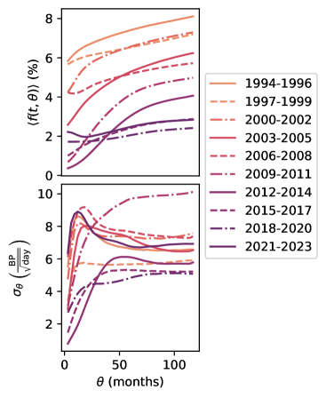
Figure 2: Unconditional mean and volatility of forward rates per tenor $\theta$ across each of the three-year periods in our sample.

Central to the present study, the empirical Pearson correlations $\hat{\rho}_{\theta\theta^{\prime}}$ among the daily forward rate increments of tenor $\theta$ and $\theta^{\prime}$ are depicted in Fig. 3 for the specific period $2021-2023$. As noted by Baaquie and Bouchaud [1], these correlations form a very smooth surface – necessitating the introduction of a stiffness term in Eq. (II), without which this surface would exhibit a cusp singularity along the diagonal. Note furthermore that the curvature along the diagonal decreases as the tenor $\theta$ increases which, as alluded to above, did motivate the introduction of a perceived, “psychological time”.

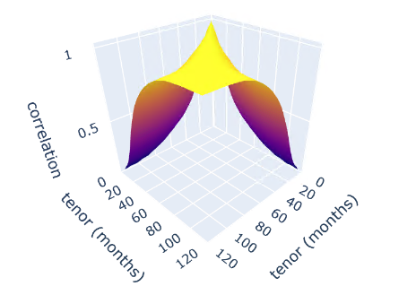
Figure 3: Empirical Pearson correlation surface between the daily forward rate increments of different tenors $\theta,\theta^{\prime}$ for the period $2021-2023$. Notice that the surface is smooth across the diagonal $\theta=\theta^{\prime}$, with a curvature that decreases with $\theta.$

V.2 Calibration over the whole sample

We fit our micro-founded three parameter discrete model BBD3 (using Eq. (27)) to the observed correlation matrix over the period $1994-2023$, defining our whole sample. For this purpose, we define the error variance $\Sigma^{2}$ by

$$\Sigma^{2}:=\frac{1}{n^{2}}\sum_{\theta,\theta^{\prime}}\left(\mathcal{E}_{\theta\theta^{\prime}}-\frac{1}{n^{2}}\sum_{\theta,\theta^{\prime}}\mathcal{E}_{\theta\theta^{\prime}}\right)^{2},$$ (28)

where $\mathcal{E}_{\theta\theta^{\prime}}=\rho_{\theta\theta^{\prime}}-\hat{\rho}_{\theta\theta^{\prime}}$ is the difference between modelled and empirical correlations for the forward rates of tenor $\theta$ and $\theta^{\prime}$. We will refer to $\Sigma$ as the typical error of fit. We will use this indicator to assess the accuracy of our model.

The minimization of the error variance $\Sigma^{2}$ yields an optimal set of parameters ${\bf{p}}^{*}=(\psi^{*},\mu^{*},\nu^{*})$ for the period $1994-2023$. The results in Fig. 4 represent such a fit along the largest anti-diagonal direction and gives the typical error over the whole surface, showing the high accuracy of the BBD3 model. We find the optimal parameters $\psi^{*}=2.06$ months, $\mu^{*}=1.06$, and $\nu^{*}=2.21$, for which $\Sigma=1.47\%$.

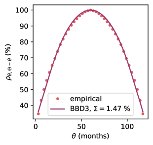
Figure 4: Dots represent the empirical correlation $\rho_{\theta\theta^{\prime}}$ along the longest stretch perpendicular to the diagonal, i.e. $\theta^{\prime}=\Theta-\theta$ , where $\Theta$ is the maximum available maturity. The plain lines are the best fit for our micro-founded three parameter discrete model BBD3 (using Eq. (27)) for the period $1994-2023$.

V.3 A two-parameter version

The interpretation of the discrete model in terms of a mean reverting force driving back tenor $\theta$ to the average of its two nearby tenors $\theta\pm 1$ suggests that the discrete fourth order derivative may in fact not be needed, i.e. that one can set $\nu=\infty$. This effectively reduces the number of parameters to just two, $\psi$ and $\mu$, a version of the model that we will call BBD2.

The calibration of BBD2 fully vindicates the above intuition: we find that the optimal values of the parameters over the full sample are given by $\psi^{*}=2.00$ months and $\mu^{*}=1.01$, corresponding to a typical error $\Sigma$ of $1.52$ %, only $5$ basis points larger than to the one found for BBD3 with one less parameter. In view of this, we restrict to the more parsimonious version BBD2 in the following, where we calibrate the model independently on each three-year sub-period.

V.4 BBD2 calibration on separate three-year periods

Fig. 5 represent the largest anti-diagonal of the fit of the BB2 model over the whole correlation surface, for each three-year sub-period. The typical error and calibrated parameters for these intervals, detailed in Figure 6, demonstrate the relative stability of the parameters throughout the assessed periods. However, periods characterized by significant monetary policy shifts exhibit a decrease in line tension (reflected in higher $\mu$ values) and goodness-of-fit (higher typical error $\Sigma$). Specifically, four periods present line tension lower than its long-term value: (i) the $2006-2008$ interval, marked by substantial central bank rate cuts during the financial crisis; (ii) the $2009-2011$ span, during the first and second rounds of Quantitative Easing, with the Federal Reserve purchasing $900$ billion dollars in US treasury bonds; (iii) the $2012-2014$ phase, with an additional $800$ billion in bond purchases (third Quantitative Easing); and (iv) the $2021-2023$ period, notable for the fourth Quantitative Easing amid the COVID-19 pandemic. This suggests that asset purchase programs induce periods of heightened curvature on the forward rate curve, i.e. more decoupling between nearby tenor. Finally, the two periods that include the financial crisis($2006-2008$ and $2009-2011$) are associated with the highest concavity of the psychological time (lowest levels of $\psi$), indicating a more myopic perception of time in financial markets under stress.

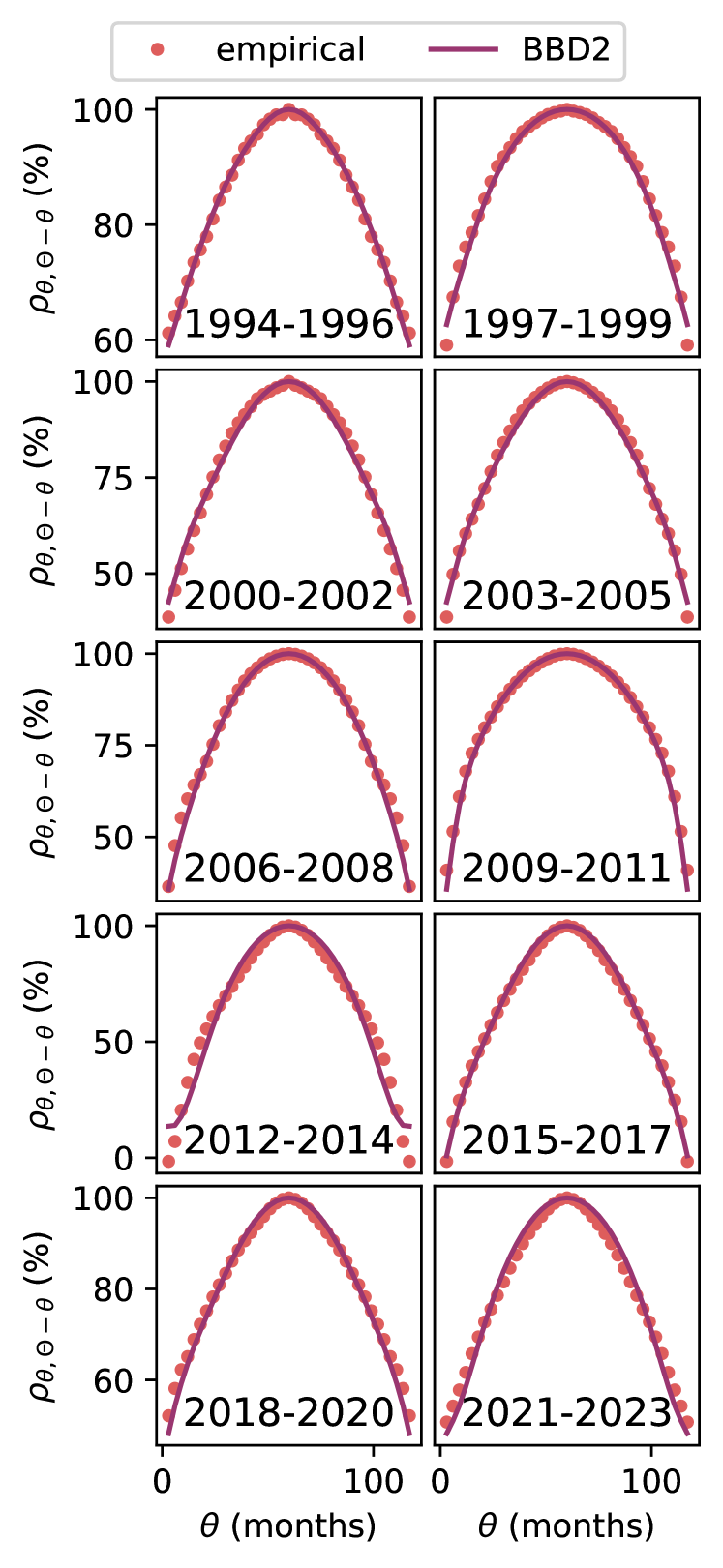
Figure 5: Dots represent the empirical correlation $\rho_{\theta\theta^{\prime}}$ along the longest stretch perpendicular to the diagonal, i.e. $\theta^{\prime}=\Theta-\theta$ , where $\Theta$ is the maximum available maturity. The plain lines are the best fit for our micro-founded discrete model BBD2 (using Eq. (27)). It is clear from these plots that BBD2 provides very accurate fits for all sub-periods, except 2009-2014.

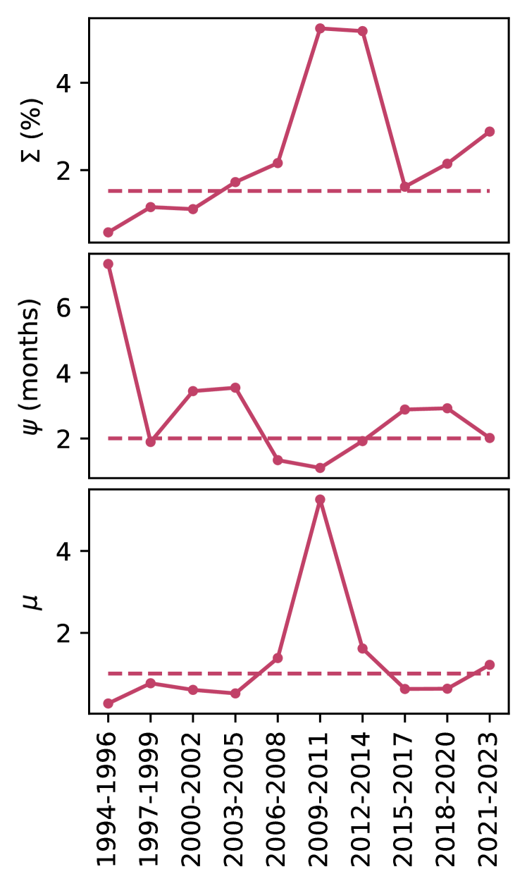
Figure 6: Optimal typical error and fitted parameters obtained with our two-parameter micro-founded discrete model BBD2, Eq. (27) with $\nu=\infty$. The dotted lines corresponds to the calibration results on the $1994-2023$ period. Note that the typical error $\Sigma$ yielded by the fit on the whole sample is not equal to the average error across sub-periods.

V.5 BBD2 sloppiness analysis

We define the Hessian matrix $\mathcal{H}$ as the second-order derivative of the typical error $\Sigma$, computed at the optimal set of parameters ${\bf{p}}^{*}$, i.e.

$$\mathcal{H}_{ij}:=p^{*}_{i}p^{*}_{j}\left.\frac{\partial^{2}\Sigma}{\partial p_{i}\partial p_{j}}\right|_{p_{i}=p^{*}_{i},p_{j}=p^{*}_{j}}$$ (29)

The eigenvalues $\lambda=(\lambda_{1},\lambda_{2})$ and eigenvectors ${\bf{e}}$ of the Hessian matrix $\mathcal{H}$ are presented in Fig. 7 for the BBD2 model. Note that $\lambda_{1}\gg\lambda_{2}$, which means that only the combination of parameters along the ${\bf{e}}_{1}$ direction is relevant, the other direction being “sloppy” (see for example Brown and Sethna [57], Waterfall et al. [58], Gutenkunst et al. [59]). Fig. 7 reveals that the main sensitivity mode of the BBD2 model is a roughly equal combination of the parameters $\psi$ and $\mu$.

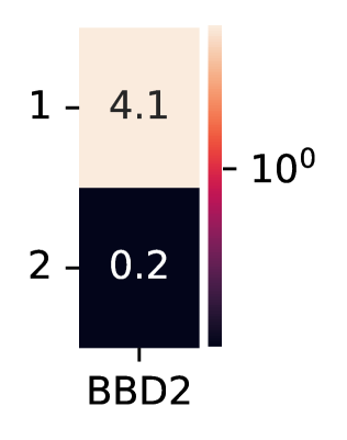
(a) Eigenvalues $\lambda_{1,2}$

(b) Eigenvectors ${\bf{e}}_{1,2}$

Figure 7: Eigenvalues $\lambda$ and eigenvectors ${\bf{e}}$ of the Hessian matrix at ${\bf{p}}^{*}$ in the BBD2 model.

V.6 Comparison with Baaquie and Bouchaud [1]

We show in Appendix E that the continuous BBL model (Baaquie-Bouchaud model with logarithmic psychological time, Eq. (61)) achieves a very high global accuracy with $\Sigma=1.01\%$, compared to $1.52\%$ for BBD2 and $1.47\%$ for BBD3.

However, removing the stiffness term now considerably degrades the goodness-of-fit, which increases the typical error $\Sigma$ from $1.01\%$ to $4.06\%$. As obvious from Appendix E.5, Fig. 13, this is chiefly because the correlation surface develops a cusp around the diagonal $\theta=\theta^{\prime}$, which was actually the very reason why Baaquie and Bouchaud [1] introduced such a stiffness term!

The discrete BBD2 model therefore appears superior not only because it is micro-founded and intuitively compelling, but also because it is more parsimonious: it naturally gets rid of the diagonal cusp without having to introduce any additional parameter. The discrete second derivative $f_{\theta+1}+f_{\theta-1}-2f_{\theta}$ indeed formally contains continuous derivatives $\partial_{\theta}^{2k}f(\theta)$ of all even orders, and is therefore sufficient to regularize the correlation function across the diagonal.

In Appendix E we also discuss the alternative version of our model (using Eq. (27) with $\mathcal{D}_{1}$ instead of $\mathcal{D}_{2}$), which leads to almost identical results to the BBD model, see Figure 12.

VI The Epps effect

An important vindication of our framework, in particular the dynamical construction of field $A_{\theta}$ using Eq. (11), is our ability to account for the so-called Epps effect [37] in a very natural way.

Indeed, the auto-covariance of $\Delta A/\sqrt{\Delta t}$ is predicted by the theory to increase from $0$ for $\Delta t\to 0$ at fixed $\tau$, to $2D\,\mathcal{D}_{2}(\theta,\theta^{\prime})$ when $\Delta t\gg\tau$, see Eq. (46) for details.

Without modifying our model at the daily time scale, we may postulate that an additional, small white noise contributes to $A_{\theta}$, originating for example from the idiosyncratic dynamics of order flow. We shall assume that the variance of such a noise is $2D\varepsilon\Delta t$, with $\varepsilon$ an extra $\theta$ independent parameter such that $\varepsilon\ll\mathcal{D}_{2}$. We then obtain the following scale-dependent covariance structure for $\Delta A$:

$$\langle\Delta A_{\theta}(t)\Delta A_{\theta^{\prime}}(t)\rangle=\left\{\begin{aligned} &2D\varepsilon\,\delta_{\theta\theta^{\prime}}\,\Delta t+O(\Delta t^{2})&\text{ for }\Delta t\ll\tau,\\ &2D\,\mathcal{D}_{2}(\theta,\theta^{\prime})\,\Delta t&\text{ for }\Delta t\gg\tau,\end{aligned}\right.$$ (30)

that we can compare with empirical data. Each colored line in Fig. 8 represents the correlation $\rho_{\theta\theta^{\prime}}$ across different time scales $\Delta t$ among pairs of forward rate variations $(\Delta f_{\theta},\Delta f_{\theta^{\prime}})$, as given by our model (see Eq. (46)) calibrated on daily correlations (see section V.2) with the additional fitting parameter $\varepsilon$ set to $0.02$ ($\mathcal{D}_{2}(\theta,\theta)$ is in the range of $0.28$ to $0.43$).

Fig. 8 clearly demonstrates that our model is able to reproduce the whole dependence of the empirical correlations of pairs of SOFR Futures binned at different time scales (black and grey curves). In fact, one can back out from this exercice the correlation time scale $\tau$ through a minimization of the differences between empirical and theoretical correlations across time scales. This leads to a very reasonable value $\tau\approx 13$ minutes that can be interpreted as the information propagation time along the FRC.

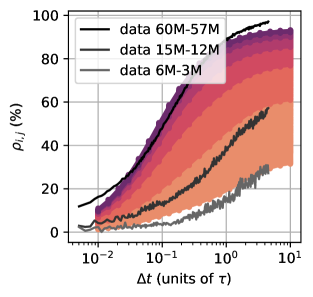
Figure 8: Colored lines: theoretical Pearson correlation coefficients among pairs of forward rate variations $(\Delta f_{\theta},\Delta f_{\theta^{\prime}})$ as a function of the time scale $\Delta t$ (see (46)). Each color correspond to a pair ordered from lowest (orange) to the hightest (purple) correlation level at the time scale $\Delta t=10\tau$ ($\tau=13$ minutes). The parameter $\varepsilon$ of the idiosyncratic white noise is set to $0.02$. Black and grey lines: empirical Pearson correlation coefficients for $3$ pairs of SOFR Futures prices for the year $2021$ at time scales ranging from $4$ seconds to one hour.

VII Conclusion

In this paper, we have reformulated the forward interest rate field theory of Baaquie and Bouchaud [1] to account in a unified manner for two important features: (a) the discrete set of traded maturities and (b) the scale dependent structure of the correlation matrix across maturities (the Epps effect). Both points are related to market mechanisms underlying our modelling assumptions.

Indeed, we believe that the emergent correlation structure is a result of market participants reacting to high frequency shocks affecting the different tenors along the forward rate curve, which get corrected in time and transmitted along maturities through a self-referential mechanism. Intuitively, the dynamics of rates maturing at $t+\theta$ in the future cannot be decoupled from rates maturing at $t+\theta^{\prime}$ when $|\theta-\theta^{\prime}|$ is small. This is encoded, within our framework, via relative mean-reverting forces proportional to the discrete Laplacian and discrete fourth derivative of the returns along the maturity axis. As it turns out, the discrete fourth derivative plays a minor role and can be neglected – whereas this term was crucial in the continuous time version of Baaquie and Bouchaud [1].

We have shown that such a parsimonious specification, further equipped with the notion of “psychological time” that shrinks the perceived distance between far away maturities, allows one to reproduce remarkably well (with an error below $2\%$) the full correlation structure of the forward rate curve, in particular the maturity dependent curvature of the correlation perpendicular to the diagonal $\theta=\theta^{\prime}$. The obtained parameters are found to be stable and reasonable across most of the tested periods. Quite remarkably, we find that the data is compatible with the assumption of a logarithmic dependence of the perceived time as a function of real time, which translates into the hyperbolic discounting factor advocated in the behavioural economics literature [2]. From our calibration to the data, we find that the cross-over time between normal time flow and logarithmic time flow occurs around 2 months in the future. This also means that a year ten years from now is perceived by the bond markets as one week in real time. This is quite an extreme distortion of future time that reflects the extremely myopic nature of financial markets.

Finally, our approach also quantitatively reproduces the empirical finding of negligible correlations at high frequencies [37], which slowly build up at lower frequencies, see Fig. 8. The modeling framework we advocate also captures several phenomena consistent with the market micro-structure literature, including (i) non-martingality of prices at short time scales and (ii) price-impact and cross-impact effects. These phenomena that will be detailed in a companion paper Le Coz et al. [40].

VIII Acknowledgments

We would like to express our gratitude to Michael Benzaquen, Damien Challet and Iacopo Mastromatteo, who contributed to our research through fruitful discussions. We are also indebted to Bertrand Hassani, who provided us with the opportunity to conduct this study at Quant AI Lab.

This research was conducted within the Econophysics & Complex Systems Research Chair, under the aegis of the Fondation du Risque, the Fondation de l’École polytechnique, the École polytechnique and Capital Fund Management.

Appendix A Notations

Table 1 summarises the notations used in this study.

Expression	Definition
$n$	The number of available SOFR futures.
$t$	The current time.
$T$	The maturity.
$P(t,T)$	The price at time t of a zero-coupon bond maturing at $T$.
$\theta$	The time-to-maturity or tenor, in units of 3 months.
$f(t,\theta)$	The value at time t of the instantaneous forward rate of tenor $\theta$ (continuous notation).
$f_{\theta}(t)$	The value at time t of the instantaneous forward rate of tenor $\theta$ (discrete notation).
$A(t,\theta)$	The driftless correlated noise field (continuous notation).
$A_{\theta}(t)$	The driftless correlated noise field (discrete notation).
$\eta(t,\theta)$	The two-dimensional white noise on continuous space.
$\eta_{\theta}(t)$	The discrete white noise of tenor $\theta$.
$\sigma(t,\theta)$	The volatility at time $t$ of the infinitesimal variation of the instantaneous forward rate of time-to-maturity $\theta$ (continuous notation).
$\sigma_{\theta}(t)$	The volatility at time $t$ of the infinitesimal variation of the instantaneous forward rate of time-to-maturity $\theta$ (discrete notation).
$\gamma(t,\theta)$	The drift at time $t$ of the infinitesimal variation of the instantaneous forward rate of time-to-maturity $\theta$ (continuous notation).
$\gamma_{\theta}(t)$	The drift at time $t$ of the infinitesimal variation of the instantaneous forward rate of time-to-maturity $\theta$ (discrete notation).
$\mu$	The line tension parameter.
$\nu$	The stiffness (or bending rigidity) parameter.
$\mathcal{D}_{BB}(\theta,\theta^{\prime})$	The Baaquie-Bouchaud correlator [1].
$\tau$	The time scale for the emergence of correlations.
$\Delta t$	The time scale at which forward variations are observed, corresponding to one day unless specified otherwise.
$\Delta\eta_{\theta}$	The coarse-grained cumulative sum over the time scale $\Delta t$ of the two-dimensional white noise $\eta_{\theta}$.
$\Delta A_{\theta}$	The coarse-grained cumulative sum over the time scale $\Delta t$ of the correlated noise field $A_{\theta}$.
$\Delta f_{\theta}$	The forward rate increments over the time scale $\Delta t$.
$\langle.\rangle$	The average operator over the functional weight $e^{S[A]}$.
$\delta(.)$	The Dirac delta function.
$\delta_{\theta\theta^{\prime}}$	The Kronecker delta.
$\mathcal{L}[.]$	The continuous linear differential operator on space.
$\mathcal{L}_{d}[.]$	The discrete linear differential operator on space.
$L_{d}[.]$	The Fourier transform of the discrete linear differential operator on space.
$G_{\theta\theta^{\prime}}(.)$	Green function or propagator of the discretized Eq. (13)
$\mathcal{D}_{2}(\theta,\theta^{\prime})$	The spatial correlator in the discrete BBD model.
$\mathcal{D}_{1}(\theta,\theta^{\prime})$	The spatial correlator in the discrete BBDSR model.
$z(\theta)$	The psychological time.
$\psi$	The psychological time parameter in the change of variable $z(\theta)=\psi\log\left(1+\frac{\theta}{\psi}\right)$.
$\bar{\psi}$	The psychological time parameter in the change of variable $\bar{z}(\theta)=\theta^{\bar{\psi}}$ [1].
$2D\Delta t$	The variance of $\Delta\eta$.
$2D\epsilon\Delta t$	The variance of the cumulative sum of the idiosyncratic two-dimensional white noise.
$\mathcal{F}[f]$	The Fourier transform of the function of the maturity $\theta\mapsto f(\theta)$.
$\Sigma$	The typical error between the empirical and the modelled correlations.

Table 1: Notations

Appendix B Solution to the Discretized Master Equation

We define the propagator $\mathcal{G}_{\theta\theta^{\prime}}(t,t^{\prime})$ as the solution to

$$\frac{\partial\mathcal{G}}{\partial t}+\frac{1}{\tau}\mathcal{L}_{d}[\mathcal{G}]=\delta(t-t^{\prime})\delta_{\theta\theta^{\prime}}.$$ (31)

The symmetry of the functions $\theta\mapsto\mathcal{L}_{d}[\mathcal{G}]_{\theta}(t)$ and $\theta\mapsto\delta_{\theta\theta^{\prime}}$ indicates that $\mathcal{G}_{\theta\theta^{\prime}}(t,t^{\prime})$ depends only on $|\theta-\theta^{\prime}|$ and $t-t^{\prime}$. Let $H$ deonote the Heaviside function. Applying discrete Fourier decomposition to the dimension $\theta-\theta^{\prime}$ yields a particular solution:

$$\mathcal{F}[\mathcal{G}](\xi,t-t^{\prime})=H(t-t^{\prime})e^{-\frac{L_{d}(\xi)(t-t^{\prime})}{\tau}},$$ (32)

where $L_{d}(\xi)=1+2\frac{(1-\cos{\xi})}{\mu^{2}}+4\frac{(1-\cos{\xi})^{2}}{\nu^{4}}$ and $\mathcal{F}[\mathcal{G}](\xi,t-t^{\prime})$ denote the spatial Fourier transform of $\mathcal{L}_{d}[A]_{\theta}(t)$ and $\mathcal{G}_{\theta\theta^{\prime}}(t-t^{\prime})$ respectively. These functions are continuous in $\xi$ and $t$.

Seeking a solution on $\mathbb{R}\times\mathbb{Z}$ for the discretized Eq. (13) without boundary conditions, we extend the noise $\eta$ so that $\eta_{\theta}(t)=0$ for $\theta\in\mathbb{Z}_{-}^{*}$. The solution is

$$\mathcal{A}_{\theta}(t) =\frac{1}{\tau}\int_{\mathbb{R}}{\rm d}t^{\prime}\sum_{\theta^{\prime}=-\infty}^{+\infty}\mathcal{G}_{|\theta-\theta^{\prime}|}(t-t^{\prime})\eta_{\theta^{\prime}}(t^{\prime})$$

$$=\frac{1}{\tau}\int_{-\infty}^{t}{\rm d}t^{\prime}\sum_{\theta^{\prime}=0}^{+\infty}\mathcal{G}_{|\theta-\theta^{\prime}|}(t-t^{\prime})\eta_{\theta^{\prime}}(t^{\prime}).$$ (33)

Similarly, $\mathcal{A}_{-\theta}(t)$ solves the discretized Eq. (13) without boundary conditions when substituting $\eta_{\theta}(t)$ with $\eta_{-\theta}(t)$. Thus, a specific solution on $\mathbb{R}\times\mathbb{Z}_{+}$ that satisfies the Neumann boundary condition is

$$A_{\theta}(t):=\mathcal{A}_{\theta}(t)+\mathcal{A}_{-\theta}(t).$$ (34)

The propagator $G_{\theta\theta^{\prime}}(t-t^{\prime})$ associated with this solution is defined as

$$G_{\theta\theta^{\prime}}(t-t^{\prime}):=\mathcal{G}_{|\theta-\theta^{\prime}|}(t-t^{\prime})+\mathcal{G}_{\theta+\theta^{\prime}}(t-t^{\prime})$$

$$=\frac{1}{2\pi}\int_{-\pi}^{\pi}{\rm d}\xi\left(e^{i\xi(\theta-\theta^{\prime})}+e^{i\xi(\theta+\theta^{\prime})}\right)\mathcal{F}[\mathcal{G}](\xi,t-t^{\prime}).$$ (35)

For consistency with the centered discretization scheme, the inverse Fourier transform is centered on $[-\pi,+\pi]$.

Appendix C Noise correlators

C.1 Autocovariance of the correlated noise

The autocovariance of $A$ is defined by

$$\langle A_{\theta}(t)A_{\theta^{\prime}}(t^{\prime})\rangle:=\frac{1}{\tau^{2}}\int_{-\infty}^{t}{\rm d}u\int_{-\infty}^{t^{\prime}}{\rm d}v$$ (36)

$$\sum_{(U,V)\in\mathbb{N}^{2}}G_{\theta U}(t-u)G_{\theta^{\prime}V}(t^{\prime}-v)\left\langle\eta_{U}(u)\eta_{V}(v)\right\rangle.$$

Recalling that

$$\left\langle\eta_{U}(u)\eta_{V}(v)\right\rangle=2D\delta(u-v)\delta_{UV},$$ (37)

we derive

$$\langle A_{\theta}(t)A_{\theta^{\prime}}(t^{\prime})\rangle$$

$$=\frac{2D}{\tau^{2}}\int_{-\infty}^{t\wedge t^{\prime}}{\rm d}u\sum_{U\in\mathbb{N}}G_{\theta U}(t-u)G_{\theta^{\prime}U}(t^{\prime}-u).$$ (38)

Substituting the propagator $G$ with its expression in Eq. (B) yields

$$\langle A_{\theta}(t)A_{\theta^{\prime}}(t^{\prime})\rangle$$

$$=\frac{2D}{(2\pi\tau)^{2}}\iint_{-\pi}^{\pi}{\rm d}\xi{\rm d}\xi^{\prime}\int_{-\infty}^{t\wedge t^{\prime}}{\rm d}ue^{-\frac{1}{\tau}\left(L_{d}(\xi)(t-u)+L_{q^{\prime}}(t^{\prime}-u)\right)}$$

$$\hskip 28.45274pt\sum_{U\in\mathbb{N}}\left(e^{i\xi(\theta-U)}+e^{i\xi(\theta+U)}\right)\left(e^{i\xi^{\prime}(\theta^{\prime}-U)}+e^{i\xi^{\prime}(\theta^{\prime}+U)}\right)$$

$$=\frac{2D}{(2\pi\tau)^{2}}\iint_{-\pi}^{\pi}{\rm d}\xi{\rm d}\xi^{\prime}\int_{-\infty}^{t\wedge t^{\prime}}{\rm d}ue^{-\frac{1}{\tau}\left(L_{d}(\xi)(t-u)+L_{d}(\xi^{\prime})(t^{\prime}-u)\right)}$$

$$\hskip 85.35826pte^{i(\xi\theta+\xi^{\prime}\theta^{\prime})}\sum_{U\in\mathbb{N}}\left(e^{iU(\xi+\xi^{\prime})}+e^{iU(\xi-\xi^{\prime})}\right)$$

$$=\frac{D}{\pi\tau^{2}}\int_{-\pi}^{\pi}{\rm d}\xi\int_{-\infty}^{t\wedge t^{\prime}}{\rm d}ue^{-\frac{L_{d}(\xi)}{\tau}\left(t+t^{\prime}-2u\right)}\left(e^{i\xi(\theta-\theta^{\prime})}+e^{i\xi(\theta+\theta^{\prime})}\right),$$

having noted that $L_{d}(-\xi)=L_{d}(\xi)$. The computation of the integral with respect to time gives the expression of the autocovariance of $A$:

$$\langle A_{\theta}(t)A_{\theta^{\prime}}(t^{\prime})\rangle$$

$$=\frac{D}{2\pi\tau}\int_{-\pi}^{\pi}{\rm d}\xi\frac{e^{i\xi(\theta-\theta^{\prime})}+e^{i\xi(\theta+\theta^{\prime})}}{L_{d}(\xi)}e^{-\frac{L_{d}(\xi)}{\tau}|t-t^{\prime}|}.$$ (39)

We now define the quantity $\mathcal{D}_{1}(\theta,\theta^{\prime})$ by

$$\mathcal{D}_{1}(\theta,\theta^{\prime})=\frac{1}{2\pi}\int_{-\pi}^{\pi}{\rm d}\xi\frac{e^{i\xi(\theta-\theta^{\prime})}+e^{i\xi(\theta+\theta^{\prime})}}{L_{d}(\xi)}.$$ (40)

$L_{d}(\xi)$ is symmetric, so one can reformulate the above quantity as

$$\mathcal{D}_{1}(\theta,\theta^{\prime})=\frac{1}{\pi}\int_{0}^{\pi}{\rm d}\xi\frac{2\cos{\xi\theta}\cos{\xi\theta^{\prime}}}{L_{d}(\xi)}.$$ (41)

Therefore, for $\tau$ close to $0$, the covariance of $A$ simplifies to

$$\langle A_{\theta}(t)A_{\theta^{\prime}}(t^{\prime})\rangle=\left\{\begin{aligned} &0,\text{ if }t\neq t^{\prime},\\ &\frac{D}{\tau}\mathcal{D}_{1}(\theta,\theta^{\prime}),\text{ if }t=t^{\prime}.\end{aligned}\right.$$ (42)

In our case, $L_{d}(\xi)=1+2\frac{1-\cos{\xi}}{\mu^{2}}+4\frac{(1-\cos{\xi})^{2}}{\nu^{4}}$. Hence, one can show that, for $\xi\ll 1$ and $\tau\ll 1$, the autocovariance $\langle A_{\theta}(t)A_{\theta^{\prime}}(t^{\prime})\rangle$ converges to the correlator $\delta(t-t^{\prime})\mathcal{D}_{BB}(\theta,\theta^{\prime})$ introduced by Baaquie and Bouchaud [1].

C.2 Autocovariance of cumulative correlative noise

We define the coarse-grained cumulative sum of $A_{\theta}$ over a time interval $\Delta t\gg\tau$ by

$$\Delta A_{\theta}=\int_{t-\Delta t/2}^{t+\Delta t/2}A_{\theta}(u){\rm d}u.$$ (43)

We derive the autocovariance of $\Delta A$

$$\langle\Delta A_{\theta}(t)\Delta A_{\theta^{\prime}}(t^{\prime})\rangle=\int_{t-\Delta t/2}^{t+\Delta t/2}{\rm d}u\int_{t^{\prime}-\Delta t/2}^{t^{\prime}+\Delta t/2}{\rm d}v\langle A_{\theta}(u)A_{\theta^{\prime}}(v)\rangle,$$

$$=\frac{D}{2\pi\tau}\int_{-\pi}^{\pi}{\rm d}\xi\int_{t-\Delta t}^{t}{\rm d}u\int_{t^{\prime}-\Delta t}^{t^{\prime}}{\rm d}v$$

$$\hskip 85.35826pt\frac{e^{i\xi(\theta-\theta^{\prime})}+e^{i\xi(\theta+\theta^{\prime})}}{L_{d}(\xi)}e^{-\frac{L_{d}(\xi)}{\tau}|u-v|}.$$ (44)

We now define the quantity $\mathcal{D}_{2}(\theta,\theta^{\prime})$ by

$$\mathcal{D}_{2}(\theta,\theta^{\prime}) =\frac{1}{2\pi}\int_{-\pi}^{\pi}{\rm d}\xi\frac{e^{i\xi(\theta-\theta^{\prime})}+e^{i\xi(\theta+\theta^{\prime})}}{[L_{d}(\xi)]^{2}},$$

$$=\frac{1}{\pi}\int_{0}^{\pi}{\rm d}\xi\frac{2\cos{\xi\theta}\cos{\xi\theta^{\prime}}}{[L_{d}(\xi)]^{2}}.$$ (45)

If $t=t^{\prime}$, the expression of $\langle\Delta A_{\theta}(t)\Delta A_{\theta^{\prime}}(t^{\prime})\rangle$ becomes

$$\langle\Delta A_{\theta}(t)\Delta A_{\theta^{\prime}}(t)\rangle$$ (46)

$$=\frac{D}{\pi}\int_{-\pi}^{\pi}{\rm d}\xi\frac{e^{i\xi(\theta-\theta^{\prime})}+e^{i\xi(\theta+\theta^{\prime})}}{[L_{d}(\xi)]^{2}}\left\{\Delta t+\frac{\tau}{L_{d}(\xi)}\right.$$

$$\hskip 142.26378pt\left.\left(e^{-\frac{L_{d}(\xi)}{\tau}\Delta t}-1\right)\right\},$$

$$\xrightarrow[\tau\mapsto 0]{}2D\Delta t\mathcal{D}_{2}(\theta,\theta^{\prime}).$$

Note that in the other limit $\Delta t\ll\tau$, one finds that

$$\langle\Delta A_{\theta}(t)\Delta A_{\theta^{\prime}}(t)\rangle\approx D\frac{\Delta t^{2}}{\tau}\mathcal{D}_{1}(\theta,\theta^{\prime})$$ (47)

This encodes the Epps effect: correlations tend to zero at very small time resolutions.

Otherwise, if $|t-t^{\prime}|>\Delta t$, we obtain

$$\langle\Delta A_{\theta}(t)\Delta A_{\theta^{\prime}}(t^{\prime})\rangle$$

$$=-\frac{\tau D\Delta t}{\pi}\int_{-\pi}^{\pi}{\rm d}\xi\frac{e^{i\xi(\theta-\theta^{\prime})}+e^{i\xi(\theta+\theta^{\prime})}}{[L_{d}(\xi)]^{3}}\hskip 85.35826pt$$

$$\hskip 85.35826pt\left(e^{-\frac{L_{d}(\xi)}{\tau}(t-t^{\prime})}+e^{-\frac{L_{d}(\xi)}{\tau}(t-t^{\prime}-\Delta t)}\right)$$

$$\xrightarrow[\tau\mapsto 0]{}0$$ (48)

Hence, for $\tau$ close to $0$, the covariance of $\Delta A$ can be written as

$$\langle\Delta A_{\theta}(t)\Delta A_{\theta^{\prime}}(t^{\prime})\rangle=\left\{\begin{aligned} &0,\text{ if }|t-t^{\prime}|>\Delta t,\\ &2D\Delta t\mathcal{D}_{2}(\theta,\theta^{\prime}),\text{ if }t=t^{\prime}.\end{aligned}\right.$$ (49)

Appendix D Closed formulas for the correlators

We perform a rotation of the tenors $\theta$ and $\theta^{\prime}$ in order to formulate our model in relation to the diagonal and anti-diagonal elements of the variance-covariance matrix.

$$\left\{\begin{aligned} &\theta_{+}=\theta+\theta^{\prime},\\ &\theta_{-}=\theta-\theta^{\prime},\end{aligned}\right.$$ (50)

For integer $\theta$’s, a second change of variable $z=e^{i\xi}$ allows us to write $\mathcal{D}_{k}$ as a contour integral

$$\mathcal{D}_{k}(\theta_{+};\theta_{-})=\frac{\nu^{4}}{2\pi}\int_{\gamma(1)}\frac{z^{|\theta_{-}|+1}+z^{\theta_{+}+1}}{P(z)^{k}},$$ (51)

where $P(z)=z^{2}-z\left(\frac{z-1}{\mu}\right)^{2}+\left(\frac{z-1}{\nu}\right)^{4}$ and $\gamma(1)$ is the unit circle. The residue theorem then yields

$$\mathcal{D}_{1}(\theta,\theta^{\prime})=\nu^{4}\frac{(\beta^{+}_{-})^{|\theta_{-}|+1}+(\beta^{+}_{-})^{\theta_{+}+1}}{(\beta^{+}_{-}-\beta_{+}^{+})(\beta^{+}_{-}-\beta^{-}_{+})(\beta^{+}_{-}-\beta_{-}^{-})}$$

$$+\nu^{4}\frac{(\beta_{-}^{-})^{|\theta_{-}|+1}+(\beta_{-}^{-})^{\theta_{+}+1}}{(\beta_{-}^{-}-\beta_{+}^{+})(\beta_{-}^{-}-\beta_{+}^{-})(\beta_{-}^{-}-\beta_{-}^{+})},$$ (52)

where,

$$\beta^{+}_{\pm}=1+\frac{\alpha_{+}\pm\sqrt{\alpha_{+}(\alpha_{+}+4)}}{2},$$

$$\beta^{-}_{\pm}=1+\frac{\alpha_{-}\pm\sqrt{\alpha_{-}(\alpha_{-}+4)}}{2},$$

$$\alpha_{\pm}=\frac{\nu^{4}}{2\mu^{2}}\left(1\pm\sqrt{1-4\left(\frac{\mu}{\nu}\right)^{4}}\right).$$ (53)

Similarly, one computes $\mathcal{D}_{2}(\theta,\theta^{\prime})$ thanks to the residue theorem:

$$\mathcal{D}_{2}(\theta,\theta^{\prime})=\text{Res}(g,\beta^{+}_{-})+\text{Res}(g,\beta_{-}^{-}),$$ (54)

where $g(z)=\nu^{8}\frac{z^{|\theta_{-}|+3}+z^{\theta_{+}+3}}{P(z)^{2}}$ and the residuals $\text{Res}(g,\beta^{+}_{-})$ and $\text{Res}(g,\beta_{-}^{-})$ at the poles $\beta^{+}_{-}$ and $\beta^{-}_{-}$ are given by

$$\text{Res}(g,\beta^{+}_{-})=\nu^{8}\frac{(\beta^{+}_{-})^{|\theta_{-}|+2}+(\beta^{+}_{-})^{\theta_{+}+2}}{(\beta^{+}_{-}-\beta_{+}^{+})^{2}(\beta^{+}_{-}-\beta^{-}_{+})^{2}(\beta^{+}_{-}-\beta_{-}^{-})^{2}}$$

$$\hskip 56.9055pt+\nu^{8}\frac{(\beta^{+}_{-})^{|\theta_{-}|+3}+(\beta^{+}_{-})^{\theta_{+}+3}}{(\beta^{+}_{-}-\beta_{+}^{+})^{3}(\beta^{+}_{-}-\beta^{-}_{+})^{3}(\beta^{+}_{-}-\beta_{-}^{-})^{3}}$$

$$\hskip 56.9055pt\left((\beta^{+}_{-}-\beta^{-}_{+})(\beta^{+}_{-}-\beta^{-}_{-})+(\beta^{+}_{-}-\beta^{+}_{+})(\beta^{+}_{-}-\beta^{-}_{-})\right.$$

$$\hskip 56.9055pt\left.+(\beta^{+}_{-}-\beta^{+}_{+})(\beta^{+}_{-}-\beta^{-}_{+})\right),$$ (55)

and by

$$\text{Res}(g,\beta^{-}_{-})=\nu^{8}\frac{(\beta^{-}_{-})^{|\theta_{-}|+2}+(\beta^{-}_{-})^{\theta_{+}+2}}{(\beta^{-}_{-}-\beta_{+}^{+})^{2}(\beta^{-}_{-}-\beta^{-}_{+})^{2}(\beta^{-}_{-}-\beta^{+}_{-})^{2}}$$

$$\hskip 56.9055pt+\nu^{8}\frac{(\beta^{-}_{-})^{|\theta_{-}|+3}+(\beta^{-}_{-})^{\theta_{+}+3}}{(\beta^{-}_{-}-\beta_{+}^{+})^{3}(\beta^{-}_{-}-\beta^{-}_{+})^{3}(\beta^{-}_{-}-\beta^{+}_{-})^{3}}$$

$$\hskip 56.9055pt\left((\beta^{-}_{-}-\beta^{-}_{+})(\beta^{-}_{-}-\beta^{+}_{-})+(\beta^{-}_{-}-\beta^{+}_{+})(\beta^{-}_{-}-\beta^{+}_{-})\right.$$

$$\hskip 56.9055pt\left.+(\beta^{-}_{-}-\beta^{+}_{+})(\beta^{-}_{-}-\beta^{-}_{+})\right).$$ (56)

Appendix E Comparison with alternative models

In this appendix, we present and compare the performance of two additional models: (i) the regularized version of the continuous model from Baaquie and Bouchaud [1]; and (ii) an alternative version of our micro-founded discrete model, BBD. Additionally, we evaluate the two-parameter versions of these models.

E.1 The Baaquie-Bouchaud Discrete, Square-Root

As mentioned in section IV.3, an alternative specification of our micro-founded model is to define a linear operator $\tilde{\mathcal{L}}={\mathcal{L}}^{1/2}$ in Eq. (13). For such a specification, the equal-time Pearson correlation is given by

$$\tilde{\rho}_{\theta\theta^{\prime}}=\frac{\mathcal{D}_{1}(z(\theta),z(\theta^{\prime}))}{\sqrt{\mathcal{D}_{1}(z(\theta),z(\theta))\mathcal{D}_{1}(z(\theta^{\prime}),z(\theta^{\prime}))}},$$ (57)

a result we will refer to as BBDSR3, for Baaquie-Bouchaud Discrete, Square-Root, three parameters.

E.2 The Baaquie-Bouchaud, Logarithm

The stiff propagator BB04 model [1] proposed the change of variable $\bar{z}(\theta)=\theta^{\bar{\psi}}$. As mentioned in section IV.2, this formulation violate the constaint that for very small maturities psychological time and real time should become equivalent. In addition, this change is variable is mis-specified for $\psi$ close to zero. Indeed, for fixed $\theta$

$$\bar{z}(\theta)\xrightarrow[\psi\mapsto 0]{}1.$$ (58)

Remediating these two limitations requires introducing two parameters, $\psi$ and $\zeta$, in the definition of the psychological time:

$$\bar{z}(\theta)=\frac{\psi}{\zeta}\left(\left(1+\frac{\theta}{\psi}\right)^{\zeta}-1\right),$$ (59)

where ${\psi}$ has dimensions of time and $\zeta$ is a pure number $\leq 1$. For this new change of variable $\bar{z}(\theta)$ is equivalent to $\theta$ for $\theta$ approaching $0$, proportional to $\theta^{\zeta}$ for large values of $\theta$, and equal to $\theta$ for $\zeta=1$. Moreover, for $\zeta$ approaching $0$,

$$\bar{z}(\theta)\approx\psi\log{\left(1+\frac{\theta}{\psi}\right)}=z(\theta)$$ (60)

Actually, we found that the calibration of the BB04 with the change of variable $\bar{z}$ yields an optimal value for $\zeta$ very close to $0$. Hence we define a regularized version of the BB04 model by replacing $\bar{z}(\theta)$ by $z(\theta)$. For such a specification, the equal-time Pearson correlation is given by

$$\tilde{\rho}_{\theta\theta^{\prime}}=\frac{\mathcal{D}_{BB}(z(\theta),z(\theta^{\prime}))}{\sqrt{\mathcal{D}_{BB}(z(\theta),z(\theta))\mathcal{D}_{BB}(z(\theta^{\prime}),z(\theta^{\prime}))}},$$ (61)

a result we will refer to as BBL3 model for Baaquie-Bouchaud, Logarithm, three parameters.

E.3 Calibration over the whole sample

Table 2 presents the optimal calibrated parameters when fitting these models to empirical Pearson correlations for the period $1994-2023$. The discrete models BBD3 and BBDSR3 both yield a psychological time parameter $\psi\approx 2$ months, implying that bond markets perceive a year a decade ahead as approximately one week in real time. In contrast, the BBL model suggests a lower value for $\psi$ (0.7 months, corresponding to approximately 20 calendar days), meaning that a year in ten years is perceived as two days in physical time, a scenario that seems quite improbable. Additionally, the three models suggest plausible tension $\mu$ and stiffness $\nu$ parameters.

Model	$\psi^{*}$ (months)	$\mu^{*}$	$\nu^{*}$
BBL3	0.671	1.90	3.42
BBD3	2.06	1.02	2.21
BBDSR3	2.01	0.78	0.98

Table 2: Optimal parameters obtained when fitting the tested models to empirical Pearson correlations for the period $1994-2023$. Three models are considered: (i) the continuous regularized model BBL (Eq. (61)); our micro-founded discrete model BBD (Eq. (27)); and (iii) the BBDSR model (Eq. (57)). While $\mu$ and $\nu$ are dimensionless in the discrete models, these parameters are in $\text{3 months}^{-1}$ in the case of the BBL3 model.

Fig. 9 represents the correlations, along the largest anti-diagonal direction, generated by the calibration of these three models on the period $1994-2023$. This figure also shows the typical error computed over the whole surface, exhibiting the high accuracy of the tested models.

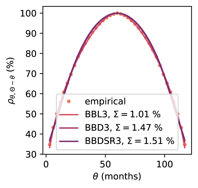
Figure 9: Dots represent the empirical correlation $\rho_{\theta\theta^{\prime}}$ along the longest stretch perpendicular to the diagonal, i.e. $\theta^{\prime}=\Theta-\theta$ , where $\Theta$ is the maximum available maturity. The plain lines are the best fit for: (i) the regularized version BBL3 of the continuous model [1], using Eq. (61); our micro-founded discrete model BBD3, using Eq. (27); (iii) the BBDSR3 model, using Eq. (57).

E.4 Stability analysis

In this section, we evaluate the stability of the three-parameter models over successive three-year intervals within our dataset. Direct calibration to the correlation structure of the FRC results in volatile, and at times, unrealistic parameter estimates. To mitigate this, we analyze the Hessian matrix for the optimally calibrated parameter set $\bf{p}^{*}$ over the entire $1994-2023$ period. As delineated in section V.5, only the combination of parameters along the first eigenvector ${\bf{e}}_{1}$ of the Hessian is relevant, the other two directions being “sloppy” (see for example Brown and Sethna [57], Waterfall et al. [58], Gutenkunst et al. [59]). Accordingly, we compute the goodness-of-fit for each three-year segment along $\bf{e}_{1}$. More precisely, we compute the typical error $\Sigma$ for a set of parameters defined by

$${\bf{p}}={\bf{p}}^{*}+x{\bf{e}}_{1}$$ (62)

where $x$ measures the relative displacement from ${\bf{p}}^{*}$. By design, the typical error reaches its minimum for $x=0$ for the aggregate period, confirming $\bf{p}^{*}$ as the optimal parameter set. For other periods, slight adjustments along $\bf{e}_{1}$ enhance the model fit. We have neglected the possibility of ever slightly improving the fit by moving in directions ${\bf e}_{2}$ and ${\bf e}_{3}$. We define the optimal parameters for each period as those that minimize the error along $\bf{e}_{1}$.

Fig. 12 displays the typical error and calibrated parameters across various models and periods, illustrating a consistent fit quality except during significant monetary policy shifts (refer to Section V.4). It also indicates that this calibration approach ensures parameter stability for all models. Notably, the $\nu$ parameter in BBD3 exhibits greater stability than in BBDSR3, as indicated by its lower weighting in $\mathbf{e}_{1}$ of the Hessian matrix (Figure 11). Conversely, the BBDSR3 model shows greater stability in the $\mu$ parameter. Thus, both micro-founded models, BBD3 and BBDSR3, demonstrate comparable stability. The main eigenvector of the BBL3 model’s Hessian matrix, associated with the largest eigenvalue, is predominantly influenced by $\psi$, leading to the most stable estimates for $\mu$ and $\nu$. However, the values derived for the psychological time parameter $\psi$ in this model are implausibly low.

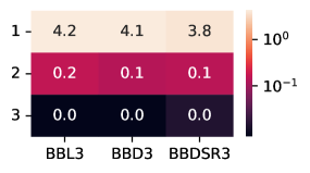
Figure 10: Eigenvalues of the Hessian matrix at ${\bf{p}}^{*}$ in: (i) the continuous regularized model BBL3 (Eq. (61)); (ii) our micro-founded discrete model BBD3 (Eq. (27)); and (iii) the BBDSR3 model (Eq. (57)). The first direction is one order of magnitude more significant than the two other ones.

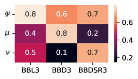
Figure 11: First eigenvector ${\bf{e}}_{1}$ of the Hessian matrix at ${\bf{p}}^{*}$ in: (i) the continuous regularized model BBL3 (Eq. (61)); (ii) our micro-founded discrete model BBD3 (Eq. (27)); and (iii) the BBDSR3 model (Eq. (57)).

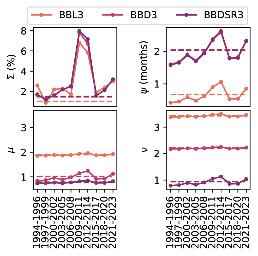
Figure 12: Typical error and fitted parameters within: (i) the continuous regularized model BBL3 (Eq. (61)); (ii) our micro-founded discrete model BBD3 (Eq. (27)); and (iii) the BBDSR3 model (Eq. (57)). The dotted lines correspond to the calibration results on the $1994-2023$ period for each model. While $\mu$ and $\nu$ are dimensionless in the discrete models, these parameters are in $\text{3 months}^{-1}$ in the case of the BBL3 model.

E.5 Two-parameter versions

In this section, we compare the performances of the two-parameter variants of our models by assigning to the stiffness parameter $\nu$ an infinite value. This adjustment applies to: (i) the regularized version BBL3 of the continuous model from [1], using Eq. (61); (ii) our micro-founded discrete model BBD3, using Eq. (27); and (iii) our alternative BBDSR3 model, using Eq. (57). These models are denoted as BBL2, BBD2, and BBDSR2, respectively.

Optimal calibration parameters, obtained by fitting these models to empirical Pearson correlations for the period $1994-2023$, are displayed in Table 3. The BBD2 and BBDSR2 models present similar and plausible values for the psychological time and line tension parameters. In contrast, the BBL2 model results in improbable values for $\psi$ and $\mu$. As previously mentioned, this is primarily because the correlation surface develops a cusp around the diagonal $\theta=\theta^{\prime}$, which was actually the very reason why Baaquie and Bouchaud [1] introduced the stiffness term $\nu$.

Model	$\psi^{*}$ (months)	$\mu^{*}$
BBL2	$1.27\times 10^{-5}$	$5.21\times 10^{4}$
BBD2	$2.00$	$1.01$
BBDSR2	$2.01$	$0.509$

Table 3: Optimal parameters obtained when fitting the tested models to empirical Pearson correlations for the period $1994-2023$. Three models are considered: (i) the continuous regularized model BBL2 (Eq. (61) with $\nu=\infty$); our micro-founded discrete model BBD2 (Eq. (27) with $\nu=\infty$); and (iii) the BBDSR2 model (Eq. (57) with $\nu=\infty$). While $\mu$ is dimensionless in the discrete models, this parameter is in units of $\text{3 months}^{-1}$ in the case of the BBL2 model.

Figure 13 depicts the correlation coefficients along the most extended anti-diagonal for the period $1994-2023$ as determined by the calibration of the BBL2, BBD2, and BBDSR2 models. It also illustrates the typical error across the correlation surface, underscoring the superior precision of the BBD2 model relative to the continuous variant. Additionally, Figure 14 indicates that BBD2 exhibits greater parameter stability across sub-periods than its continuous counterparts.

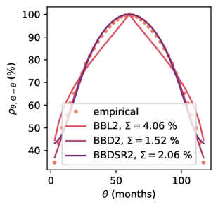
Figure 13: Dots represent the empirical correlation $\rho_{\theta\theta^{\prime}}$ along the longest stretch perpendicular to the diagonal, i.e. $\theta^{\prime}=\Theta-\theta$ , where $\Theta$ is the maximum available maturity. The plain lines are the best fit for: (i) the regularized version BBL2 of the continuous model [1], using Eq. (61) with $\nu=\infty$; our micro-founded discrete model BBD2, using Eq. (27) with $\nu=\infty$; (iii) the BBDSR2 model, using Eq. (57) with $\nu=\infty$.

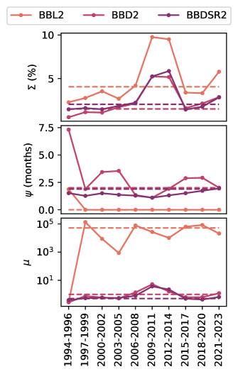
Figure 14: Typical error and fitted parameters within: (i) the continuous regularized model BBL2 (Eq. (61) with $\nu=\infty$); (ii) our micro-founded discrete model BBD2 (Eq. (27) with $\nu=\infty$); and (iii) the BBDSR2 model (Eq. (57) with $\nu=\infty$). The dotted lines correspond to the calibration results on the $1994-2023$ period for each model. While $\mu$ is dimensionless in the discrete models, this parameter is in units of $\text{3 months}^{-1}$ in the case of the BBL2 model.

Appendix F Curvature along the anti-diagonals

One of the most salient success of the BB04 model is its ability, in line with observations, to reproduce the power-law decay of the curvature of forward rate correlations perpendicular to the diagonal. Fig. 15 shows estimations of the curvatures generated by the tested models and the ones empirically observed. These estimations are produced through the fitting of parabolas using $10$ points around the center of each anti-diagonal of the correlation surface for the $1994-2023$ period. Fig. 15 reveals the adequacy of the continuous model BBL3, and the discrete models, BBD3 and BBD2, with the observed curvature.

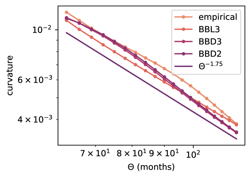
Figure 15: Curvature of the correlation surface along the stretches perpendicular to the diagonal, i.e. $\theta^{\prime}=\Theta-\theta$ as a function of largest tenor $\Theta$ for the $1994-2023$ period. Three models are compared: (i) the continuous regularized model BBL3 (Eq. (61)); (ii) our micro-founded discrete model BBD3 (Eq. (27)); and (iii) the two-parameter model BBD2 (Eq. (27) with $\nu=\infty$).

References

- Baaquie and Bouchaud [2004] B. Baaquie and J.-P. Bouchaud, Wilmott Magazine , 2 (2004).
- Farmer and Geanakoplos [2009] J. D. Farmer and J. Geanakoplos, Hyperbolic Discounting Is Rational: Valuing the Far Future with Uncertain Discount Rates, Cowles Foundation Discussion Papers (Cowles Foundation for Research in Economics, Yale University, 2009).
- Hull [2018] J. Hull, Options, Futures, and Other Derivatives, tenth edition ed. (Pearson, Chennai, 2018).
- Brigo and Mercurio [2006] D. Brigo and F. Mercurio, Interest Rate Models — Theory and Practice: With Smile, Inflation and Credit (Springer International Publishing, 2006).
- Bachelier [1900] L. Bachelier, Annales scientifiques de l’École normale supérieure 17, 21 (1900).
- Osborne [1959] M. F. M. Osborne, Operations Research 7, 145 (1959).
- Black and Scholes [1973] F. Black and M. Scholes, Journal of Political Economy 81, 637 (1973).
- Heston [1993] S. L. Heston, Review of Financial Studies 6, 327 (1993).
- Bacry et al. [2001] E. Bacry, J. Delour, and J. F. Muzy, Physical Review E 64, 026103 (2001).
- Gatheral et al. [2014] J. Gatheral, T. Jaisson, and M. Rosenbaum, arXiv:1410.3394 [q-fin] (2014), arXiv:1410.3394 [q-fin] .
- Zumbach [2010] G. Zumbach, Quantitative Finance 10, 431 (2010).
- Dandapani et al. [2021] A. Dandapani, P. Jusselin, and M. Rosenbaum, Quantitative Finance 21, 1235 (2021).
- Wu et al. [2022] P. Wu, J.-F. Muzy, and E. Bacry, Physica A: Statistical Mechanics and its Applications 604, 127919 (2022), arXiv:2201.09516 [q-fin] .
- Bouchaud et al. [1999] J.-P. Bouchaud, N. Sagna, R. Cont, N. El-Karoui, and M. Potters, Applied Mathematical Finance 6, 209 (1999).
- Santa-Clara and Sornette [2001] P. Santa-Clara and D. Sornette, Review of Financial Studies 14, 149 (2001).
- Heath et al. [1992] D. Heath, R. Jarrow, and A. Morton, Econometrica 60, 77 (1992).
- Hughston [1996] L. Hughston, ed., Vasicek and beyond: Approaches to Building and Applying Interest Rate Models (Risk Books, London, 1996).
- Björk [2019] T. Björk, Arbitrage Theory in Continuous Time, 4th ed. (Oxford University Press, 2019).
- Kennedy [1994] D. P. Kennedy, Mathematical Finance 4, 247 (1994).
- Kennedy [1997] D. P. Kennedy, Mathematical Finance 7, 107 (1997).
- Cont [2005] R. Cont, International Journal of Theoretical and Applied Finance 08, 357 (2005).
- Goldstein [2000] R. S. Goldstein, Review of Financial Studies 13, 365 (2000).
- Baaquie [2001] B. E. Baaquie, Physical Review E 64, 016121 (2001).
- Baaquie [2002] B. E. Baaquie, Physical Review E 65, 056122 (2002).
- Baaquie [2004] B. E. Baaquie, Quantum Finance: Path Integrals and Hamiltonians for Options and Interest Rates, 1st ed. (Cambridge University Press, 2004).
- Bueno-Guerrero et al. [2015] A. Bueno-Guerrero, M. Moreno, and J. F. Navas, Physica A: Statistical Mechanics and its Applications 433, 229 (2015).
- Bueno-Guerrero et al. [2016] A. Bueno-Guerrero, M. Moreno, and J. F. Navas, Physica A: Statistical Mechanics and its Applications 461, 217 (2016).
- Bueno-Guerrero et al. [2020] A. Bueno-Guerrero, M. Moreno, and J. F. Navas, Physica A: Statistical Mechanics and its Applications 559, 125103 (2020).
- Bueno-Guerrero et al. [2022] A. Bueno-Guerrero, M. Moreno, and J. F. Navas, Quantitative Finance 22, 197 (2022).
- Baaquie [2007] B. E. Baaquie, Physical Review E 75, 016703 (2007).
- Baaquie [2009] B. E. Baaquie, Physical Review E 80, 046119 (2009).
- Baaquie [2010] B. E. Baaquie, Physica A: Statistical Mechanics and its Applications 389, 296 (2010).
- Baaquie [2018] B. E. Baaquie, Quantum Field Theory for Economics and Finance, 1st ed. (Cambridge University Press, 2018).
- Baaquie and Tang [2012] B. E. Baaquie and P. Tang, Physica A: Statistical Mechanics and its Applications 391, 1287 (2012).
- Baaquie and Liang [2007] B. E. Baaquie and C. Liang, Physical Review E 75, 016704 (2007).
- Wu and Xu [2014] T. L. Wu and S. Xu, Journal of Futures Markets 34, 580 (2014).
- Epps [1979] T. W. Epps, Journal of the American Statistical Association 74, 291 (1979).
- Renò [2003] R. Renò, International Journal of Theoretical and Applied Finance 06, 87 (2003).
- Toth and Kertesz [2009] B. Toth and J. Kertesz, Quantitative Finance 9, 793 (2009).
- Le Coz et al. [2024] V. Le Coz, I. Mastromatteo, and M. Benzaquen, arXiv (2024).
- Baaquie and Srikant [2004] B. E. Baaquie and M. Srikant, Physical Review E 69, 036129 (2004).
- Green et al. [1994] L. Green, A. F. Fry, and J. Myerson, Psychological Science 5, 33 (1994).
- Sozou [1998] P. D. Sozou, Proceedings of the Royal Society of London. Series B: Biological Sciences 265, 2015 (1998).
- Frederick et al. [2002] S. Frederick, G. Loewenstein, and T. O’donoghue, Journal of Economic Literature 40, 351 (2002).
- Green and Myerson [2004] L. Green and J. Myerson, Psychological Bulletin 130, 769 (2004).
- Thaler [2005] Thaler, Advances in Behavioral Finance. 2 (Russell Sage Foundation [u.a.], New York, 2005).
- Dasgupta and Maskin [2005] P. Dasgupta and E. Maskin, American Economic Review 95, 1290 (2005).
- Kim and Zauberman [2009] B. K. Kim and G. Zauberman, Journal of Neuroscience, Psychology, and Economics 2, 91 (2009).
- Ray and Bossaerts [2011] D. Ray and P. Bossaerts, Frontiers in Neuroscience 5, 10.3389/fnins.2011.00002 (2011).
- Cui [2011] X. Cui, Frontiers in Integrative Neurosci 5, 10.3389/fnint.2011.00024 (2011).
- Bouchaud and Potters [2003] J.-P. Bouchaud and M. Potters, Theory of Financial Risk and Derivative Pricing: From Statistical Physics to Risk Management, 2nd ed. (Cambridge University Press, 2003).
- Matacz and Bouchaud [2000a] A. Matacz and J.-P. Bouchaud, International Journal of Theoretical and Applied Finance 03, 703 (2000a).
- Matacz and Bouchaud [2000b] A. Matacz and J.-P. Bouchaud, International Journal of Theoretical and Applied Finance 03, 381 (2000b).
- Amin and Morton [1994] K. I. Amin and A. J. Morton, Journal of Financial Economics 35, 141 (1994).
- Hull and White [1994] J. C. Hull and A. D. White, The Journal of Derivatives 2, 37 (1994).
- Fabozzi and Mann [2005] F. J. Fabozzi and S. V. Mann, eds., The Handbook of Fixed Income Securities, 7th ed. (McGraw-Hill, New York, 2005).
- Brown and Sethna [2003] K. S. Brown and J. P. Sethna, Physical Review E 68, 021904 (2003).
- Waterfall et al. [2006] J. J. Waterfall, F. P. Casey, R. N. Gutenkunst, K. S. Brown, C. R. Myers, P. W. Brouwer, V. Elser, and J. P. Sethna, Physical Review Letters 97, 150601 (2006).
- Gutenkunst et al. [2007] R. N. Gutenkunst, J. J. Waterfall, F. P. Casey, K. S. Brown, C. R. Myers, and J. P. Sethna, PLoS Computational Biology 3, e189 (2007).