Multiple Model Reference Adaptive Control with Blending for Non-Square Multivariable Systems

Abstract

In this paper we develop a multiple model reference adaptive controller (MMRAC) with blending. The systems under consideration are non-square, i.e., the number of inputs is not equal to the number of states; multi-input, linear, time-invariant with uncertain parameters that lie inside of a known, compact, and convex set. Moreover, the full state of the plant is available for feedback. A multiple model online identification scheme for the plant’s state and input matrices is developed that guarantees the estimated parameters converge to the underlying plant model under the assumption of persistence of excitation. Using an exact matching condition, the parameter estimates are used in a control law such that the plant’s states asymptotically track the reference signal generated by a state-space model reference. The control architecture is proven to provide boundedness of all closed-loop signals and to asymptotically drive the state tracking error to zero. Numerical simulations illustrate the stability and efficacy of the proposed MMRAC scheme.

I Introduction

The use of multiple models to describe the dynamics of uncertain systems has been studied [1, 2, 3, 4], and shown to improve the transient-time performance [5], the steady-state tracking performance [4, 6], and robustness [7] when compared to a single model approach. Multiple model control techniques can be broadly divided into switching control, which allows for the selection of a best model in different dynamic situations [8, 7], and blending control, where the information from different models is combined to get a single description of the system [9, 10, 3, 11]. In this paper we opt for a blending technique since it allows for better closed-loop performance when compared to any single model technique [12], and avoids possible undesirable transient-time behavior that switching control may exhibit [13, 14].

Multiple model approaches with blending have various promising applications in identification and control of time-varying (TV) systems, including adaptive identification of MIMO, linear, periodically TV systems (with known period) [15] and improvement of the transients and adaptation speed in adaptive control of uncertain, TV, MIMO systems [9]. The stability and robustness properties were studied in [3]. Mixing adaptive techniques have also been used to achieve faster tracking for a class of nonlinear discrete-time systems [16]. For the case of experimental results, the use of mixing control has allowed to decrease overshoots, settling time, steady state error [17, 18], and designing fault tolerant controllers [10]. Other applications include multiple model estimation of power systems models [19], development of an adaptive controller for partially-observed Boolean dynamical systems [20], and distributed state estimation using a network of local sensors [21].

Model reference control has been rigorously and methodically studied for many years and proposes promising applications with detailed design procedures. When we consider systems with uncertainty, model reference adaptive controllers (MRAC) are a versatile technique that achieves robust and satisfactorily closed-loop performances [22, 23]. The combination of MRAC with multiple model approaches to obtain a continuous input signal calculated using all the identification errors from all the models is studied in [1, 24]. Similar work is present in [25], where adaptive identification models are considered instead of fixed models. In [9], a similar identification scheme is integrated with linear quadratic optimal controllers to design a multiple MRAC (MMRAC) scheme for tracking reference signals generated by a linear reference model. The asymptotic tracking of the MMRAC scheme for linear, time-invariant (LTI), MIMO systems is proven and simulations are presented to evaluate and validate the performance.

In this paper we consider non-square, multi-input, LTI systems with polytopic parameter uncertainty, whose unknown plant models are in the interior of the convex hull of a finite number of fixed models. Based on full state measurements, we develop a parameter identification scheme that estimates a weight vector which determines the convex combination that yields the state-space representation of the uncertain system.

This paper extends our previous work [26] in several significant ways. The systems under consideration do not have to be square, i.e., the number of inputs can be less or equal to the number of states. Moreover, unlike in [26], in this article the number of fixed models that define the polytopic uncertainty of the plant can be arbitrary. This relaxation allows us to develop a procedure to obtain a set of fixed corner systems to use in the identification process. Furthermore, we provide sufficient conditions under which the parameter estimates asymptotically converge to the plant’s uncertain parameters. The simulations presented here point to faster convergence of the parameter estimates to their true values, making the state error of the proposed MMRAC scheme also converge faster compared to a single model MRAC approach.

The problem formulation is presented in Section II, together with the assumptions. In Section III, we present a selection process for the corner systems. In Section IV, we present the identification scheme with its stability analysis. We use these results in Section V to develop the MMRAC scheme. A set of simulations are presented comparing the MMRAC scheme to the single model case for uncertain systems tracking references in Section VI using MATLAB and Simulink based simulations. We finalize with the conclusions in Section VII.

Notation

If $S\subset\mathbb{R}^{n}$, then $\operatorname{conv}\left(S\right)$ denotes the closed convex hull of $S$, the interior of $S$ is written $\operatorname{int}(S)$. Let $\|\cdot\|$ denote the 2-norm of both vectors and matrices. The kernel of a matrix $A$ is denoted by $\operatorname{Ker}A$. Given two matrices $Q,R\in\mathbb{R}^{n\times n}$, we write $Q\succeq R$ if $Q-R$ is positive semi-definite. For two signals $f_{1}$ and $f_{2}$ we write $f_{1}\equiv f_{2}$, if there exist $\alpha$, $\beta>0$ such that for all $t\geq 0$, ${\|f_{1}\left(t\right)-f_{2}\left(t\right)\|\leq\beta e^{-\alpha t}}$. Further, if $e_{f}=f_{1}-f_{2}$ satisfies $\dot{e}_{f}(t)=-\alpha e_{f}(t)$ then we write $f_{1}\stackrel{{\scriptstyle\alpha}}{{=}}f_{2}$. If $x\in\mathbb{R}^{N}$, then $x_{i}$ denotes the $i$-th component, and ${\bar{x}=\left(x_{1},\cdots,x_{N-1}\right)\in\mathbb{R}^{N-1}}$. A signal $\Phi:[0,\infty)\rightarrow\mathbb{R}^{k}$ is persistently exciting (PE) if there exist $\alpha_{\Phi 1},\alpha_{\Phi 2},T_{\Phi}>0$ such that for every $t\geq 0$

$$\alpha_{\Phi 1}\mathbb{I}\preceq\int_{t}^{t+T_{\Phi}}\Phi(\tau)\Phi^{\top}(\tau)\mathrm{d}\tau\preceq\alpha_{\Phi 2}\mathbb{I}.$$ (1)

II Problem Formulation

Consider the MIMO, LTI system

$$\dot{x}_{p}\left(t\right)=A_{p}x_{p}\left(t\right)+B_{p}u\left(t\right),\>x_{p}\left(0\right)=x_{p0},\>t\geq 0,$$ (2)

where $A_{p}\in\mathbb{R}^{n\times n}$ and $B_{p}\in\mathbb{R}^{n\times m}$ are unknown constant matrices, $B_{p}$ is full column rank, $x_{p}\left(t\right)\in\mathbb{R}^{n}$, $u\left(t\right)\in\mathbb{R}^{m}$ are the state of the system and the control input, respectively. We assume that $x_{p}(t)$ is available for feedback and that the number states $n$ and inputs $m$ are known.

Remark 1

The results of this article can be applied to systems with structured uncertainties of the form ${\left(A_{p}\left(\eta\right),B_{p}\left(\eta\right)\right)}$, where ${A_{p}\left(\eta\right)\in\mathbb{R}^{n\times n}}$ and ${B_{p}\left(\eta\right)\in\mathbb{R}^{n\times m}}$ are unknown constant matrices dependent on the uncertain parameter vector ${\eta\in S\subset\mathbb{R}^{q}}$, belonging to a compact set.  $\triangle$

This article aims to design a controller such that the state $x_{p}$ of the plant (2) asymptotically tracks the signal $x_{r}$ generated by the reference model

$$\dot{x}_{r}\left(t\right)=A_{r}x_{r}\left(t\right)+B_{r}r\left(t\right),\>x_{r}\left(0\right)=x_{r0},\>t\geq 0,$$ (3)

where $A_{r}\in\mathbb{R}^{n\times n}$ and $B_{r}\in\mathbb{R}^{n\times m}$ are known constant matrices, $A_{r}$ is Hurwitz, and $r:\left[0,\infty\right)\rightarrow\mathbb{R}^{m}$ is a known, bounded, piecewise continuous reference signal. It is assumed that the plant (2) and the reference model (3) satisfy the exact matching conditions [23], as stated in the following assumption.

Assumption 1

There exist matrices $K^{*}\in\mathbb{R}^{m\times n}$ and ${L^{*}\in\mathbb{R}^{m\times m}}$ such that

$$A_{p}+B_{p}K^{*} =A_{r},$$ (4)

$$B_{p}L^{*} =B_{r}.$$ (5)

 $\triangle$

Assumption 1 is a necessary and sufficient condition to guarantee the existence of a solution to the tracking problem when the plant’s model (2) is known [23]. In addition, (5) is equivalent to $\operatorname{Im}B_{r}\subseteq\operatorname{Im}B_{p}$, which means that, without loss of generality, we can assume that $\operatorname{Im}B_{p}=\operatorname{Im}B_{r}$.

Our approach to solving the aforementioned control design problem involves online parameter identification of the system matrices $\begin{bmatrix}A_{p}&B_{p}\end{bmatrix}\eqqcolon\Theta_{p}$ by defining a compact, convex, uncertainty polytope such that for every extreme point of the polytope, also referred to as corner, there is a fixed model

$$\dot{x}_{i}(t) =A_{i}x_{i}(t)+B_{i}u(t),$$

with system matrices $\begin{bmatrix}A_{i}&B_{i}\end{bmatrix}\eqqcolon\Theta_{i}$, $i\in\left\{1,\cdots,N\right\}$. We define the set

$$\mathcal{S}\coloneqq\left\{\begin{bmatrix}A_{1}&B_{1}\end{bmatrix},\cdots,\begin{bmatrix}A_{N}&B_{N}\end{bmatrix}\right\}$$ (6)

consisting of every corner model.

Assumption 2

There exist a finite set $\mathcal{S}$ of known system matrices $\begin{bmatrix}A_{i}&B_{i}\end{bmatrix}\in\mathbb{R}^{n\times(n+m)}$, such that

1. ${\begin{bmatrix}A_{p}&B_{p}\end{bmatrix}\in\operatorname{int}\left(\operatorname{conv}\left(\mathcal{S}\right)\right)}$.

2. Every convex combination of the $B_{i}$ is full column rank.

 $\triangle$

The first item of Assumption 2 can be achieved from a system identification process which we describe in Section III-B. We require Assumption 2 (ii) to ensure that we do not have redundant inputs, or we do not drop rank of the number of inputs, losing control authority of the system. Given a set $\mathcal{S}$, there exist numerical methods to verify whether every convex combinations of the $B_{i}$’s is full rank [27].

Every point of the polytope $\operatorname{conv}\left(\mathcal{S}\right)$ can be expressed as a convex combination of the corner models $\begin{bmatrix}A_{i}&B_{i}\end{bmatrix}$, which implies that the following set is non-empty:

$$\mathcal{W}\coloneqq\left\{w\in\left[0,1\right]^{N}:\begin{bmatrix}A_{p}&B_{p}\end{bmatrix}=\sum_{i=1}^{N}w_{i}\begin{bmatrix}A_{i}&B_{i}\end{bmatrix},\sum_{i=1}^{N}w_{i}=1\right\}.$$ (7)

Consequently, the problem of identifying the unknown system matrix $\begin{bmatrix}A_{p}&B_{p}\end{bmatrix}$ is equivalent to the problem of identifying a vector $w\in\mathcal{W}$. A preliminary study of the problem with $N=n+1$, and $m=n$ was studied in [26]. In this paper unlike in [26], we study the problem for any number of inputs $m>0$, and an arbitrary number $N$ of corner models.

III Corner Model Selection

Consider a set $\mathcal{S}$ that satisfies Assumption 2 and has $N$ elements. In this section we develop a constructive procedure that, starting with $\mathcal{S}$, produces a new set

$$\mathcal{S}^{\prime}=\left\{\begin{bmatrix}A_{1}^{\prime}&B_{1}^{\prime}\end{bmatrix},\cdots,\begin{bmatrix}A^{\prime}_{N^{\prime}}&B^{\prime}_{N^{\prime}}\end{bmatrix}\right\},$$ (8)

that also satisfies Assumption 2, and such that for every $i\in\left\{1,\cdots,N\right\}$ there exist matrices $K_{i}\in\mathbb{R}^{m\times n}$ and ${L_{i}\in\mathbb{R}^{m\times m}}$ such that,

$$A_{i}^{\prime}+B_{i}^{\prime}K_{i} =A_{r},$$ (9)

$$B_{i}^{\prime}L_{i} =B_{r}.$$ (10)

III-A Satisfying the Matching Conditions for the Corner Models

In the next proposition we show how to use the information of Assumption 1 and a set $\mathcal{S}$ that satisfies Assumption 2 to obtain a new set $\mathcal{S}^{\prime}$ such that for every element of $\mathcal{S}^{\prime}$ there exist matrices $K_{i}\in\mathbb{R}^{m\times n}$ and ${L_{i}\in\mathbb{R}^{m\times m}}$ that satisfy (9) and (10).

Proposition 1

Suppose that the plant (2) and reference model (3) are such that Assumption 1 is satisfied. If there exists a set $\mathcal{S}$ that satisfies Assumption 2, then there exists a set $\mathcal{S}^{\prime}$ that also satisfies Assumption 2, and furthermore

1. $\operatorname{conv}(\mathcal{S}^{\prime})\subseteq\operatorname{conv}(\mathcal{S})$.

2. For each $i\in\left\{1,\cdots,N\right\}$, there exist matrices $K_{i}\in\mathbb{R}^{m\times n}$ and ${L_{i}\in\mathbb{R}^{m\times m}}$ such that (9) and (10) are satisfied.

Proof:

Let $(A_{p},B_{p})$ and $(A_{r},B_{r})$ be the matrix pairs that represent a plant, and a reference model, respectively. Assume that they satisfy Assumption 1. Moreover, assume that there exists a set $\mathcal{S}$ with $N$ elements that satisfies Assumption 2. The first, and trivial case, is if for every $i=1,\cdots,N$, there exist matrices $K_{i}\in\mathbb{R}^{m\times n}$ and ${L_{i}\in\mathbb{R}^{m\times m}}$ such that every corner model $[A^{\prime}_{i}~{}~{}B^{\prime}_{i}]:=[A_{i}~{}~{}B_{i}]$ satisfies (9) and (10). In that case, we can define $\mathcal{S}^{\prime}=\mathcal{S}$, and we have satisfied Assumptions 1 and 2.

For the case when there exists some $j\in\{1,\cdots,N\}$ such that $[A^{\prime}_{j}~{}~{}B^{\prime}_{j}]:=[A_{j}~{}~{}B_{j}]\in\mathcal{S}$ does not satisfy (9) or (10), consider the closed convex hull of $\mathcal{S}$, i.e., $\operatorname{conv}\left(\mathcal{S}\right).$ The set $\operatorname{conv}\left(\mathcal{S}\right)$ is a compact, convex polytope, and it is non-empty since $\begin{bmatrix}A_{p}&B_{p}\end{bmatrix}$ is an element of $\operatorname{conv}\left(\mathcal{S}\right)$ by Assumption 2 (i). Next, take the set of matrices that satisfy Equations 4 and 5:

$$\mathcal{T}\coloneqq \big{\{}\begin{bmatrix}A_{x}&B_{x}\end{bmatrix}\in\mathbb{R}^{n\times(n+m)}:$$

$$A_{x}+B_{x}K=A_{r},B_{x}L=B_{r},L\in\mathbb{R}^{m\times m},K\in\mathbb{R}^{m\times n}\big{\}}.$$

The set $\mathcal{T}$ is a hyperplane, since it can be written as $n(n+m)$ linear equations (see Section 2.2.1 of [28]), therefore it is a convex polytope. From Assumption 1, we see that if we replace $K$ and $L$ by $K^{*}$ and $L^{*}$, respectively, the element $\begin{bmatrix}A_{p}&B_{p}\end{bmatrix}$ belongs to $\mathcal{T}$, which means $\mathcal{T}$ is non-empty. The intersection set

$$\mathcal{P}\coloneqq\operatorname{conv}\left(\mathcal{S}\right)\cap\mathcal{T}.$$

is also non-empty, since $\begin{bmatrix}A_{p}&B_{p}\end{bmatrix}$ is an element of both $\operatorname{conv}\left(\mathcal{S}\right)$ and $\mathcal{T}$. Moreover, the intersection of a compact, convex polytope and a convex polytope is another compact, convex polytope (see Section 2.3.1 of [28]), which in turn implies that we can obtain $N^{\prime}$ corner models $\begin{bmatrix}A_{i}^{\prime}&B_{i}^{\prime}\end{bmatrix}$ such that

$$\mathcal{P}=\operatorname{conv}\Big{(}\underbrace{\left\{\begin{bmatrix}A_{1}^{\prime}&B_{1}^{\prime}\end{bmatrix},\cdots,\begin{bmatrix}A^{\prime}_{N^{\prime}}&B^{\prime}_{N^{\prime}}\end{bmatrix}\right\}}_{\eqqcolon\mathcal{S}^{\prime}}\Big{)}.$$

Every convex combination of the matrices $B_{i}^{\prime}$ can be written as a convex combination of the original $B_{i}$ matrices, and every convex combination of the $B_{i}$’s is full column rank, which implies that every convex combination of the $B_{i}^{\prime}$ is also full column rank. The vertices, edges and faces of $\mathcal{P}$ are obtained by intersecting the previous vertices, edges and faces from $\operatorname{conv}(\mathcal{S})$ with the set $\mathcal{T}$. Since $\begin{bmatrix}A_{p}&B_{p}\end{bmatrix}$ is not on a vertex, edge or face of $\operatorname{conv}(\mathcal{S})$ it cannot be on a vertex, edge or face of $\mathcal{P}$ and must be in the interior. Hence, the set $\mathcal{S}^{\prime}$ satisfies Assumption 2, and also every element of $\mathcal{S}^{\prime}$ satisfies (9) and (10).

∎

Remark 2

The results provided in Proposition 1 deal with systems that do not have the same number of inputs as states; the special case of $n=m$ is solved trivially, i.e. we have $\mathcal{S}=\mathcal{S}^{\prime}$. Since every convex combination of $B_{i}$ is full column rank, that means that $B_{i}$ can be inverted for all $i\in\left\{1,\cdots,N\right\}$, and the gains can be obtained as

$$K_{i} =B_{i}^{-1}(A_{r}-A_{i})$$

$$L_{i} =B_{i}^{-1}B_{r}.$$

 $\triangle$

III-B Obtaining the sets $\mathcal{S}$ and $\mathcal{S}^{\prime}$

The modeling uncertainty in (2) is taken to be parametric uncertainty in the matrices in this state-space system model. There is an implicit assumption here that the state-space system model (2) is derived from physical laws rather than from a state-space realization of an input-output system model. If we consider the maximum range of values each entry of $A_{p}$, and $B_{p}$ can take we get that we can bound $a_{ij}\in[a_{ij\min},a_{ij\max}]$ and $b_{ij}\in[b_{ij\min},b_{ij\max}]$. When we consider the minimums and maximums of every entry we write the following matrices

$$A_{p\min}\leq A_{p}\leq A_{p\max},$$

$$B_{p\min}\leq B_{p}\leq B_{p\max},$$

where $A_{p\min}$ is a matrix where each entry $a_{ij}$ takes its minimum value, and $A_{p\max}$ is a matrix where each entry $a_{ij}$ takes its maximum value, $B_{p\min}$, and $B_{p\max}$ are matrices that take the minimums and maximums of each entry $b_{ij}$, respectively, and the inequality is considered entry-wise. Let $\mathcal{S}$ be the set of all possible system matrices $\begin{bmatrix}A_{p}&B_{p}\end{bmatrix}$ each entry of which is either the corresponding entry of $[A_{p\min}~{}~{}B_{p\min}]$ or the corresponding entry of $[A_{p\max}~{}~{}B_{p\max}]$. Note that, by construction, $\mathcal{S}$ satisfies Assumption 2 (i). The number of elements in $\mathcal{S}$ is $N=2^{n(n+m)}$. If the entries can be parameterized by an uncertainty vector $\eta\in\mathbb{R}^{q}$, then $\mathcal{S}$ can be defined in terms of $2^{q}$ elements (see Remark 1).

The naïve corner model selection process described above guarantees that $\begin{bmatrix}A_{p}&B_{p}\end{bmatrix}\in\operatorname{int}\left(\operatorname{conv}\left(S\right)\right)$. However, it is not evident that Assumption 2 (ii) is satisfied. The results from [27] can be used to verify this condition. If Assumption 2 (ii) is satisfied, then the last step is to use constructive procedure from the proof of Proposition 1 to obtain $\mathcal{S}^{\prime}$.

III-C Example

In this example we consider a system with two states and one input. We assume that the plant only has uncertainty in the $B_{p}$ matrix. The unknown input matrix to the system is $B_{p}=\begin{bmatrix}2\\ 2\end{bmatrix}$. The reference models input’s matrix is $B_{r}=\begin{bmatrix}10\\ 10\end{bmatrix}$. Note that by taking $L^{*}=5$ we can satisfy (5), and Assumption 1 is satisfied. The polytopic uncertainty for $B_{p}$ is given by

$$B_{p\min}=\begin{bmatrix}1\\ 1\end{bmatrix},B_{p\max}=\begin{bmatrix}4\\ 5\end{bmatrix}.$$

Using the selection procedure from Section III-B we can take all possible combinations of the minimums and maximums of every entry of $B_{p\min}$ and $B_{p\max}$ to get

$$B_{1}=\begin{bmatrix}1\\ 1\end{bmatrix},B_{2}=\begin{bmatrix}1\\ 5\end{bmatrix},B_{3}=\begin{bmatrix}4\\ 5\end{bmatrix},B_{4}=\begin{bmatrix}4\\ 1\end{bmatrix}.$$

Since $A_{p}$ is completely known, we need to redefine the sets $\mathcal{S}$ and $\mathcal{T}$ as

$$\mathcal{S} =\left\{B_{1},\cdots,B_{4}\right\},$$

$$\mathcal{T} =\big{\{}B_{x}\in\mathbb{R}^{2\times 1}:B_{x}L=B_{r},L\in\mathbb{R}\big{\}}.$$

It is easily verifiable that $B_{p}\in\operatorname{int}\left(\operatorname{conv}\left(\mathcal{S}\right)\right)$, and that any convex combination of $B_{i}$ is full column rank. Nevertheless, if we consider $B_{2}$, $B_{3}$, or $B_{4}$ we cannot satisfy (10). Using the proof of Proposition 1 we solve for the set $\mathcal{P}$ graphically (closed line segment going from $B_{1}$ to $B_{2}^{\prime}$), as shown in Figure 1 to obtain

$$\mathcal{P}=\operatorname{conv}(\mathcal{S})\cap\mathcal{T}=\operatorname{conv}\Bigg{(}\underbrace{\left\{\begin{bmatrix}1\\ 1\end{bmatrix},\begin{bmatrix}4.5\\ 4.5\end{bmatrix}\right\}}_{\mathcal{S}^{\prime}}\Bigg{)}.$$

Note that $\begin{bmatrix}A_{p}&B_{p}\end{bmatrix}\in\operatorname{int}\left(\mathcal{P}\right)$. In addition, every convex combination of $B_{1}$ and $B_{2}^{\prime}$ is full column rank, and we can satisfy (10) with $L_{1}=10$, and $L_{2^{\prime}}=20/9$.

Figure 1: Graphic illustration of the projection process to select corner models.

IV Online Parameter Identification

Our multiple-model reference adaptive control (MMRAC) design will utilize a blending-based multiple model parameter identification (MMPI) scheme that generates estimates $\begin{bmatrix}\hat{A}_{p}(t)&\hat{B}_{p}(t)\end{bmatrix}$ of $\begin{bmatrix}A_{p}&B_{p}\end{bmatrix}$, as a weighted sum of the corner models. In this section, we provide the design, stability and convergence analysis of this MMPI scheme.

IV-A Multiple-Model Parameter Identifier Design

Filtering both sides of (2) by the linear filter $\dfrac{1}{s+\lambda}$, where $\lambda>0$ is a design parameter, we obtain the parametric model

$$z\left(t\right) \stackrel{{\scriptstyle\lambda}}{{=}}\Theta_{p}\begin{bmatrix}\phi_{1}\left(t\right)\\ \phi_{2}\left(t\right)\end{bmatrix}\eqqcolon\Theta_{p}\Phi(t),$$ (11)

where $\phi_{1}\left(t\right),z\left(t\right)\in\mathbb{R}^{n}$, $\phi_{2}\left(t\right)\in\mathbb{R}^{m}$ are generated by the filters

$$\begin{bmatrix}\dot{\phi}_{1}(t)\\ \dot{\phi}_{2}(t)\end{bmatrix} =-\lambda\begin{bmatrix}\phi_{1}(t)\\ \phi_{2}(t)\end{bmatrix}+\begin{bmatrix}x_{p}(t)\\ u(t)\end{bmatrix},\>\begin{bmatrix}\phi_{1}(0)\\ \phi_{2}(0)\end{bmatrix}=\begin{bmatrix}0\\ 0\end{bmatrix},$$

$$z(t) =\dot{\phi}_{1}(t)=-\lambda\phi_{1}(t)+x_{p}(t).$$ (12)

The relation (11) can be verified by taking time derivatives of both sides and taking the difference, i.e., (12) implies for $e_{z}(t)=z(t)-\Theta_{p}\Phi(t)$ that

$$\dot{e}_{z}(t) =\dot{z}(t)-\Theta_{p}\dot{\Phi}(t)$$

$$=-\lambda\dot{\phi}_{1}(t)+\dot{x}_{p}-\Theta_{p}\begin{bmatrix}\dot{\phi}_{1}(t)\\ \dot{\phi}_{2}(t)\end{bmatrix}$$

$$=-\lambda\dot{\phi}_{1}(t)+\Theta_{p}\begin{bmatrix}x_{p}(t)\\ u(t)\end{bmatrix}-\Theta_{p}\left(-\lambda\begin{bmatrix}\phi_{1}(t)\\ \phi_{2}(t)\end{bmatrix}+\begin{bmatrix}x_{p}(t)\\ u(t)\end{bmatrix}\right)$$

$$=-\lambda\left(-\lambda\phi_{1}(t)+x_{p}(t)\right)+\lambda\Theta_{p}\Phi(t)$$

$$=-\lambda\left(-\lambda\phi_{1}(t)+x_{p}(t)-\Theta_{p}\Phi(t)\right)$$

$$=-\lambda e_{z}(t),$$ (13)

i.e., $e_{z}(t)$ is an exponentially decaying signal.

For each of the fixed models, define

$$z_{i}\left(t\right) \coloneqq\Theta_{i}\begin{bmatrix}\phi_{1}\left(t\right)\\ \phi_{2}\left(t\right)\end{bmatrix}=\Theta_{i}\Phi(t),\>\forall i\in\left\{1,\cdots,N\right\}.$$ (14)

Then, the filtered state estimation error for each of the $N$ fixed models is defined as

$$\varepsilon_{i}\left(t\right)\coloneqq\dfrac{z\left(t\right)-z_{i}\left(t\right)}{m_{s}^{2}(t)},\forall i\in\left\{1,\cdots,N\right\},$$ (15)

where $m_{s}^{2}(t)\coloneqq 1+\alpha\|\Phi(t)\|^{2}$, $\alpha>0$, is a normalization signal which guarantees that $\dfrac{\Phi(t)}{m_{s}(t)}$ is bounded. By (7), (11)–(14), for any $w=\left[w_{1},\dots,w_{N}\right]^{\top}\in\mathcal{W}$, we obtain

$$z\left(t\right) =\sum_{i=1}^{N}w_{i}z_{i}\left(t\right)+e_{z}(t).$$ (16)

Using $\sum_{i=1}^{N}w_{i}=1$, (16) further implies

$$e_{z}(t)=\sum_{i=1}^{N}w_{i}z\left(t\right)-\sum_{i=1}^{N}w_{i}z_{i}\left(t\right) =\sum_{i=1}^{N}w_{i}\left(z\left(t\right)-z_{i}\left(t\right)\right)$$

$$=\sum_{i=1}^{N}w_{i}\varepsilon_{i}\left(t\right)m_{s}^{2}(t).$$ (17)

Adding $-\varepsilon_{N}\left(t\right)m_{s}^{2}(t)$ to both sides of (17), we obtain

$$e_{z}(t)-\varepsilon_{N}\left(t\right)m_{s}^{2}(t) =\sum_{i=1}^{N-1}w_{i}\left(\varepsilon_{i}\left(t\right)-\varepsilon_{N}\left(t\right)\right)m_{s}^{2}(t),$$

which implies, for any $w=\left[w_{1},\dots,w_{N}\right]^{\top}\in\mathcal{W}$, that

$$e_{z}(t)-\varepsilon_{N}\left(t\right)=\sum_{i=1}^{N-1}w_{i}\left(\varepsilon_{i}\left(t\right)-\varepsilon_{N}\left(t\right)\right).$$ (18)

Defining the $n\times(N-1)$ time-varying matrix

$$E\left(t\right)\coloneqq\begin{bmatrix}\varepsilon_{1}\left(t\right)-\varepsilon_{N}\left(t\right)&\cdots&\varepsilon_{N-1}\left(t\right)-\varepsilon_{N}\left(t\right)\end{bmatrix},$$ (19)

we can rewrite (18) in matrix form as

$$E\left(t\right)\bar{w}=e_{z}(t)-\varepsilon_{N}\left(t\right)$$ (20)

for any $\left[\bar{w}^{\top},w_{N}\right]^{\top}=\left[w_{1},\dots,w_{N-1},w_{N}\right]^{\top}\in\mathcal{W}$. Equation 20 motivates using the following recursive adaptive law [22] to generate estimate $\hat{w}(t)=[\hat{\bar{w}}^{\top}\left(t\right),\hat{w}_{N}\left(t\right)]^{\top}\in\mathbb{R}^{N}$, such that $\lim_{t\rightarrow\infty}\sum_{i=1}^{N}\hat{w}_{i}(t)\begin{bmatrix}A_{i}&B_{i}\end{bmatrix}=\begin{bmatrix}A_{p}&B_{p}\end{bmatrix}$.

$$\begin{split}\dot{\hat{\bar{w}}}\left(t\right)&=-\Gamma E^{\top}\left(t\right)E\left(t\right)\hat{\bar{w}}\left(t\right)-\Gamma E^{\top}\left(t\right)\varepsilon_{N}\left(t\right),\\ \hat{w}_{N}\left(t\right)&=1-\sum_{i=1}^{N-1}\hat{w}_{i}\left(t\right),\end{split}$$ (21)

where the tuning parameter $\Gamma\in\mathbb{R}^{(N-1)\times(N-1)}$ is a symmetric positive definite matrix. Let $w^{*}$ be some element in $\mathcal{W}$, and based on (21), the estimation error $\tilde{\bar{w}}\left(t\right)\coloneqq\hat{\bar{w}}\left(t\right)-\bar{w}^{*}$ satisfies

$$\dot{\tilde{\bar{w}}}\left(t\right) =\dot{\hat{\bar{w}}}\left(t\right)-\dot{\bar{w}}^{*}=\dot{\hat{\bar{w}}}\left(t\right)$$

$$=-\Gamma E^{\top}\left(t\right)E\left(t\right)\hat{\bar{w}}\left(t\right)-\Gamma E^{\top}\left(t\right)\varepsilon_{N}\left(t\right).$$ (22)

Pre-multiplying (20) by $\Gamma E^{\top}(t)$ and moving all the terms to the left hand side, we obtain

$$\Gamma E^{\top}(t)E\left(t\right)\bar{w}+\Gamma E^{\top}(t)\varepsilon_{N}\left(t\right)-\Gamma E^{\top}(t)e_{z}(t)=0$$ (23)

Adding (23) to (22), we further obtain

$$\dot{\tilde{\bar{w}}}\left(t\right) =-\Gamma E^{\top}\left(t\right)E\left(t\right)\tilde{\bar{w}}\left(t\right)-\Gamma E^{\top}(t)e_{z}(t).$$ (24)

IV-B Stability and Convergence of the Identification Process

In this subsection, we establish the stability and convergence properties of the estimation scheme (21) utilizing the following lemma.

Lemma 1 (See [22], Barbalat’s Lemma)

For a function $f:[0,\infty)\rightarrow\mathbb{R}$, if $f,\>\dot{f}\in\mathcal{L}_{\infty}$ and ${f\in\mathcal{L}_{p}}$, for some $p\in\left[1,\infty\right)$, then $\lim\limits_{t\rightarrow\infty}f\left(t\right)=0$.

The main stability and convergence properties are established in the following theorems and lemmas below.

Theorem 1

Consider the system (2) with definitions (15), and (19). Let Assumption 2 hold, $w^{*}=\left[\bar{w}^{*\top},w^{*}_{N}\right]^{\top}\in\mathcal{W}$ be an arbitrary vector within the set defined in (7), and $\tilde{\bar{w}}(t)\coloneqq\hat{\bar{w}}(t)-\bar{w}^{*}$. For any initial condition $\hat{\bar{w}}(0)\in\mathbb{R}^{N-1}$, the estimation scheme (21) guarantees that:

1. $\hat{\bar{w}}$, $\tilde{\bar{w}}$, $\dot{\tilde{\bar{w}}}$ and $E$ are bounded signals.

2. $E\tilde{\bar{w}}$ and $\dot{\tilde{\bar{w}}}$ are square integrable.

3. $\lim_{t\rightarrow\infty}E(t)\tilde{\bar{w}}(t)=0$.

4. $\hat{\bar{w}}(t)$ asymptotically converges to a constant vector $\bar{\bar{w}}\in\mathbb{R}^{N-1}$.

Proof:

Consider the Lyapunov-like function

$$V_{1}(\tilde{\bar{w}}(t),e_{z}(t))=\frac{1}{2}\tilde{\bar{w}}^{\top}(t)\Gamma^{-1}\tilde{\bar{w}}(t)+\frac{1}{2\lambda}e_{z}^{\top}(t)e_{z}(t).$$ (25)

Taking the time derivative of (25) along (24), we have

$$\dfrac{\mathrm{d}V_{1}(t)}{\mathrm{d}t} =\tilde{\bar{w}}^{\top}(t)\Gamma^{-1}\dot{\tilde{\bar{w}}}(t)+\dfrac{1}{\lambda}e_{z}^{\top}(t)\dot{e}_{z}(t)$$

$$=-\tilde{\bar{w}}^{\top}(t)\Gamma^{-1}\Gamma E^{\top}(t)E(t)\tilde{\bar{w}}(t)$$

$$-\tilde{\bar{w}}^{\top}(t)\Gamma^{-1}\Gamma E^{\top}(t)e_{z}(t)+\dfrac{1}{\lambda}e_{z}^{\top}\dot{e}_{z}$$

$$=-\tilde{\bar{w}}^{\top}(t)E^{\top}(t)E(t)\tilde{\bar{w}}(t)-\tilde{\bar{w}}^{\top}(t)E^{\top}(t)e_{z}(t)+\dfrac{1}{\lambda}e_{z}^{\top}\dot{e}_{z}$$

$$=-\dfrac{1}{2}\|E\tilde{\bar{w}}\|^{2}+\dfrac{1}{2}\|e_{z}(t)\|^{2}-\dfrac{1}{2}\|E(t)\tilde{\bar{w}}(t)+e_{z}(t)\|^{2}.$$ (26)

Since $e_{z}(t)$ is an exponentially decaying signal, Equation 26 implies that $\dot{V}_{1}$ is bounded and there exists a time instant $t_{1}>0$ such that, for all $t\geq t_{1}$, $\dot{V}_{1}(t)\leq 0$. Hence. $V_{1}$, $\tilde{\bar{w}}$, and $\hat{\bar{w}}$ are bounded. Because of normalization (15), $\varepsilon_{i}$ terms are bounded and hence $E$ is bounded, which together with (24) also implies that $\dot{\tilde{\bar{w}}}$ is bounded, finishing the proof of (i).

Since $V_{1}(t)$ is always positive, bounded, and decaying, the integral of (26) for $t=0$ to $\infty$ is finite, and hence $E\tilde{\bar{w}}$ and $E\tilde{\bar{w}}+e_{z}(t)$ are square integrable. Since $E$ is bounded, this, together with (24), further implies that $\dot{\tilde{\bar{w}}}$ is square integrable, completing the proof of (ii).

Items (i) and (ii) together with Barbalat’s Lemma imply (iii). Items (i) and (ii) further imply that $\lim_{t\rightarrow\infty}\tilde{\bar{w}}(t)$ and, hence, $\lim_{t\rightarrow\infty}\hat{\bar{w}}(t)$ exist and are finite, proving (iv). ∎

Theorem 1 implies that $\|E(t)\tilde{\bar{w}}(t)\|$ asymptotically converges to zero, but this does not mean that $\tilde{\bar{w}}(t)$ converges to the set $\mathcal{W}$. We can now state, and prove, the main result of the identification process.

Theorem 2

Consider the system (2) with definitions (15), and (19), and the estimation scheme (21). Let Assumption 2 hold, $w^{*}=\left[\bar{w}^{*\top},w^{*}_{N}\right]^{\top}\in\mathcal{W}$ be an arbitrary vector within the set defined in (7), $\tilde{\bar{w}}(t)\coloneqq\hat{\bar{w}}(t)-\bar{w}^{*}$, and $\Phi$ be bounded and satisfy the PE condition (1). Then, for any initial condition $\hat{\bar{w}}(0)\in\mathbb{R}^{N-1}$, the estimated system matrix $\sum_{i=1}^{N}\hat{w}_{i}(t)\Theta_{i}$ asymptotically converges to $\Theta_{p}$.

Proof:

Let $Q(t)\coloneqq\sum_{i=1}^{N-1}(\tilde{w}_{i}(t)(\Theta_{N}-\Theta_{i}))\in\mathbb{R}^{n\times(n+m)}$. It is easily verifiable that if $Q(t)=0$, then $\sum_{i=1}^{N}\hat{w}_{i}(t)\Theta_{i}=\Theta_{p}$, and $\hat{w}(t)\in\mathcal{W}$. Theorem 1 (iv) implies that $Q(t)$ asymptotically converges to a constant matrix $\bar{Q}\in\mathbb{R}^{n\times(n+m)}$. Hence, to establish that $\sum_{i=1}^{N}\hat{w}_{i}(t)\Theta_{i}$ asymptotically converges to $\Theta_{p}$, we will show that $\bar{Q}=0$.

Expressing Theorem 1 (iii) in summation form, we get

$$\lim_{t\rightarrow\infty}E(t)\tilde{\bar{w}}(t) =\lim_{t\rightarrow\infty}Q(t)\dfrac{\Phi(t)}{1+\alpha\|\Phi(t)\|^{2}}$$

$$=\lim_{t\rightarrow\infty}\bar{Q}\dfrac{\Phi(t)}{1+\alpha\|\Phi(t)\|^{2}}=0.$$ (27)

Since $\Phi$ is assumed to be bounded, (IV-B) implies that

$$\lim_{t\rightarrow\infty}\bar{Q}\Phi(t)=0.$$

and hence

$$\lim_{t\rightarrow\infty}\bar{Q}\Phi(t)\Phi^{\top}(t)\bar{Q}^{\top}=0.$$ (28)

Since $\Phi$ satisfies the PE condition (1), Equation (IV-B) implies that $\bar{Q}=0$, completing the proof.

∎

The recursive adaptive law (21) guarantees that $\sum_{i=1}^{N}\hat{w}_{i}\left(t\right)=1$, but not that $\hat{w}\left(t\right)\in[0,1]^{N}$. Since the set $\left[0,1\right]^{N}$ is convex, the projection of $\hat{w}\left(t\right)$ into $\left[0,1\right]^{N}$ is well-defined.

Define the compact set

$$\Pi\coloneqq\left\{\hat{\bar{w}}\in\left[0,1\right]^{N-1}:\sum_{i=1}^{N-1}\hat{\bar{w}}_{i}\leq 1\right\},$$ (29)

and let $\operatorname{Pr}_{\Pi,\hat{\bar{w}}}:\mathbb{R}^{N-1}\rightarrow\Pi\subset\mathbb{R}^{N-1}$ denote the parameter projection operator [22]. Choose $\hat{w}(0)\in\operatorname{int}(\Pi)$, then the recursive adaptive algorithm (21) with parameter projection is as follows:

$$\dot{\hat{\bar{w}}}\left(t\right) =\operatorname{Pr}_{\Pi,\hat{\bar{w}}}\left(-\Gamma\left(E^{\top}\left(t\right)E\left(t\right)\hat{\bar{w}}\left(t\right)+E^{\top}\left(t\right)\varepsilon_{N}\left(t\right)\right)\right),$$

$$\hat{w}_{N}\left(t\right) =1-\sum_{i=1}^{N-1}\hat{w}_{i}\left(t\right).$$ (30)

The parameter projection operator enforces that $\Pi$ is a positively invariant subset for the dynamics (30).

Corollary 1

The gradient adaptive law with parameter projection (30) has all the properties established in Theorem 1 for the gradient adaptive law (21). Furthermore, we get the following properties:

1. If $\hat{w}\left(0\right)\in\Pi$, then $\hat{w}\left(t\right)\in\Pi$, $\forall t\geq 0$.

2. If $\hat{w}\left(0\right)\in\operatorname{int}\Pi$, then $\hat{w}(t)$ asymptotically converges to the set $\mathcal{W}$.

Proof:

The proof follows applying Theorem 3.10.1 of [22] to (21) combined with Theorems 1 and 2. ∎

V Multiple Model Reference Adaptive Control

In this section we combine the system identification scheme of Section IV with a MMRAC controller to achieve asymptotic tracking of the reference system (3).

V-A Multiple Model Reference Adaptive Control Design

We use the recursive adaptive algorithm with parameter projection (30) to design a MMRAC scheme to achieve the adaptive state tracking control task stated in Section II. We utilize Theorem 1 (iii) to construct the proposed MMRAC scheme.

If $w\in\mathcal{W}$, then multiplying both sides of (10) by $w_{i}$ and summing over $i$ yields

$$\sum_{i=1}^{N}w_{i}B_{i}L_{i} =\sum_{i=1}^{N}w_{i}B_{r}=B_{r},$$

which implies, together with (5) from Assumption 1, that

$$B_{p}L^{*}=\sum_{i=1}^{N}w_{i}B_{i}L_{i}.$$ (31)

Applying the same steps on (9) we get

$$\begin{split}A_{r}=\sum_{i=1}^{N}w_{i}A_{r}&=\sum_{i=1}^{N}w_{i}\big{(}A_{i}+B_{i}K_{i}\big{)}\\ &=A_{p}+\sum_{i=1}^{N}w_{i}B_{i}K_{i}.\end{split}$$ (32)

Comparing (32) to (4) we get that

$$B_{p}K^{*}=\sum_{i=1}^{N}w_{i}B_{i}K_{i}.$$ (33)

Equations (31) and (33) motive us to generate estimates of the gains $K^{*}$ and $L^{*}$ using the estimates $\hat{w}\left(t\right)$, keeping in mind the rank supposition in Assumption 2, as

$$\hat{K}\left(t\right) =\hat{B}_{p}^{\dagger}(t)\sum_{i=1}^{N}\hat{w}_{i}\left(t\right)B_{i}K_{i},$$ (34)

$$\hat{L}\left(t\right) =\hat{B}_{p}^{\dagger}(t)\sum_{i=1}^{N}\hat{w}_{i}\left(t\right)B_{i}L_{i},$$ (35)

where $\hat{B}_{p}^{\dagger}(t)$ is the Moore-Penrose inverse of

$$\hat{B}_{p}(t)=\sum_{i=1}^{N}\hat{w}_{i}\left(t\right)B_{i}.$$ (36)

Equations 33, 31, 34 and 35, together with Corollary 1 further imply the following:

Corollary 2

Consider the system (2) with definitions (15), (19), and the reference model (3). If $\Phi(t)$ satisfies the PE condition with constants $\alpha_{\Phi 1}$, $\alpha_{\Phi 2}$, and $T_{\Phi}$, then the estimates $\hat{K}\left(t\right)$ and $\hat{L}\left(t\right)$ defined in (34), and (35) are bounded, and asymptotically converge to $K^{*}$ and $L^{*}$, respectively.

Proof:

Since $\Pi$ is compact, we get that $\hat{B}_{p}(t)$ belongs to a compact set, which means the Moore-Penrose inverse of $\hat{B}_{p}(t)$ exists, and it is bounded. Furthermore, from Assumption 2, we have that $\hat{B}_{p}(t)$ is full column rank, which means that we can write

$$\hat{B}_{p}^{\dagger}(t)=\left(\hat{B}_{p}^{\top}(t)\hat{B}_{p}(t)\right)^{-1}\hat{B}_{p}^{\top}(t).$$ (37)

Combining (37) with Equations 34 and 35 we get that $\hat{K}\left(t\right)$, and $\hat{L}\left(t\right)$ are bounded. The proof to show asymptotic convergence is the same as the proof for Theorem 1 (iii). ∎

The control law we will consider to achieve asymptotic tracking of the reference model is

$$u\left(t\right)\coloneqq\hat{K}\left(t\right)x_{p}\left(t\right)+\hat{L}\left(t\right)r\left(t\right).$$ (38)

V-B Stability Analysis of the Entire System

The main result of the paper is now presented.

Theorem 3

Consider the plant 2 and the reference model 3. If $\Phi(t)$ satisfies the PE condition (1), and Assumptions 2 and 1 hold, then the MMRAC scheme 12, 15, 14, 30, 34, 35, 36, 37 and 38 guarantees that for any

1. initial conditions of the plant (2),

2. initial conditions of the reference model (3), and

3. piecewise continuous and bounded reference signal ${r:\left[0,\infty\right)\rightarrow\mathbb{R}^{m}}$ in (3),

all closed-loop signals are bounded and $x_{p}\left(t\right)$ asymptotically converges to $x_{r}\left(t\right)$.

Proof:

Let $x_{p}(0)=x_{p0}$ and $x_{r}(0)=x_{r0}$ be arbitrary initial plant and reference model states, and $r(t)$ be any known, bounded, piecewise continuous reference signal. Substituting (38) into (2) we get

$$\dot{x}_{p}\left(t\right) =A_{p}x_{p}\left(t\right)+B_{p}u\left(t\right)$$

$$=A_{p}x_{p}\left(t\right)+B_{p}\hat{K}\left(t\right)x_{p}\left(t\right)+B_{p}\hat{L}\left(t\right)r\left(t\right).$$

Adding and subtracting $B_{p}K^{*}x_{p}\left(t\right)$ and $B_{p}L^{*}r\left(t\right)$, defining $\tilde{K}\left(t\right)\coloneqq\hat{K}\left(t\right)-K^{*}$, $\tilde{L}\left(t\right)\coloneqq\hat{L}\left(t\right)-L^{*}$, and using Assumption 1 we get

$$\dot{x}_{p}\left(t\right)=A_{r}x_{p}\left(t\right)+B_{r}r\left(t\right)+B_{p}\tilde{K}\left(t\right)x_{p}\left(t\right)+B_{p}\tilde{L}\left(t\right)r\left(t\right).$$

For the tracking error $e\left(t\right)\coloneqq x_{p}\left(t\right)-x_{r}\left(t\right)$, this implies

$$\dot{e}\left(t\right) =A_{r}e\left(t\right)+B_{p}\tilde{K}\left(t\right)x_{p}\left(t\right)+B_{p}\tilde{L}\left(t\right)r\left(t\right)$$

$$=\left(A_{r}+B_{p}\tilde{K}(t)\right)e(t)+B_{p}\tilde{K}(t)x_{r}(t)+B_{p}\tilde{L}(t)r(t).$$ (39)

Let $Q\in\mathbb{R}^{n\times n}$ be a fixed, symmetric, and positive definite matrix. Then we can define $P\in\mathbb{R}^{n\times n}$ to be the unique positive definite and symmetric solution of ${PA_{r}+A_{r}^{\top}P+Q=0}$. Consider the positive definite function

$$V\left(e\left(t\right)\right) =e^{\top}\left(t\right)Pe\left(t\right).$$ (40)

Taking the derivative of (40) along solutions of (39) we get

$$\dot{V}\left(e\left(t\right)\right)$$

$$=2e^{\top}\left(t\right)P\dot{e}\left(t\right)$$

$$=2e^{\top}\left(t\right)PA_{r}e\left(t\right)+2e^{\top}\left(t\right)PB_{p}\tilde{K}\left(t\right)x_{p}\left(t\right)$$

$$\qquad+2e^{\top}\left(t\right)PB_{p}\tilde{L}\left(t\right)r\left(t\right).$$ (41)

The first term satisfies

$$2e^{\top}\left(t\right)PA_{r}e\left(t\right) =e^{\top}\left(t\right)PA_{r}e\left(t\right)+e^{\top}\left(t\right)PA_{r}e\left(t\right)$$

$$=e^{\top}\left(t\right)\left(PA_{r}+A_{r}^{\top}P\right)e\left(t\right)$$

$$=-e^{\top}\left(t\right)Qe\left(t\right).$$

Hence, (41) can be rewritten as as

$$\dot{V}\left(e\left(t\right)\right)= -e^{\top}\left(t\right)Qe\left(t\right)+2e^{\top}\left(t\right)PB_{p}\tilde{K}\left(t\right)x_{p}\left(t\right)$$

$$\qquad+2e^{\top}\left(t\right)PB_{p}\tilde{L}\left(t\right)r\left(t\right).$$

Substituting $x_{p}(t)=e(t)+x_{r}(t)$, we get

$$\dot{V}\left(e\left(t\right)\right)= -e^{\top}\left(t\right)\left(Q-PB_{p}\tilde{K}\left(t\right)\right)e\left(t\right)$$

$$+2e^{\top}\left(t\right)PB_{p}\tilde{K}\left(t\right)x_{r}\left(t\right)$$

$$+2e^{\top}\left(t\right)PB_{p}\tilde{L}\left(t\right)r\left(t\right).$$

Defining

$$c_{1}(t)\coloneqq\|PB_{p}\tilde{K}(t)\|,$$

and

$$c_{2}(t)\coloneqq 2\|PB_{p}\tilde{K}(t)\|\|x_{r}(t)\|+2\|PB_{p}\tilde{L}(t)\|\|r(t)\|,$$

we have

$$\dot{V}(e(t))\leq-\left(\lambda_{\textrm{min}}(Q)-c_{1}(t)\right)\|e(t)\|^{2}+c_{2}(t)\|e(t)\|,$$ (42)

where $\lambda_{\textrm{min}}(Q)>0$ is the minimum eigenvalue of $Q$. Note that (39) does not have a finite escape time; from Corollary 2 we have that $\hat{K}(t)$ and $\hat{L}(t)$ are continuous and bounded, which means that $\tilde{K}(t)$ and $\tilde{L}(t)$ are also continuous and bounded, hence (39) may only go to infinity as time goes to infinity. Moreover, if $\Phi(t)$ is PE, then $\tilde{K}(t)$ and $\tilde{L}(t)$ converge to zero asymptotically, which lets us conclude that $c_{1}(t)$ is bounded, and there exists $t_{1}\geq 0$ such that $\lambda_{\textrm{min}}(Q)>c_{1}(t)$ for all $t\geq t_{1}$. We can define

$$\bar{c}_{1}=\sup\{c_{1}(t),t\geq t_{1}\},$$ (43)

$$\bar{c}_{2}=\sup\{c_{2}(t),t\geq t_{1}\}.$$ (44)

This implies that for all $t\geq t_{1}$ we get that if

$$\|e(t)\|>\dfrac{\bar{c}_{2}}{\lambda_{\min}Q-\bar{c}_{1}},$$

then $\dot{V}<0$, and we can conclude that $e$ is bounded. This further implies that $x_{p}$ is bounded, which finally implies that $u$ is bounded, showing that all signals in the closed-loop system are bounded. Combining this with Corollary 2 we get

$$\lim_{t\rightarrow\infty}\left(\dot{V}(e(t))+e^{\top}\left(t\right)Qe\left(t\right)\right)=0.$$

This implies that $e(t)$ converges to $0$, asymptotically, i.e., $x_{p}(t)$ asymptotically converges to $x_{r}(t)$. ∎

VI Simulations

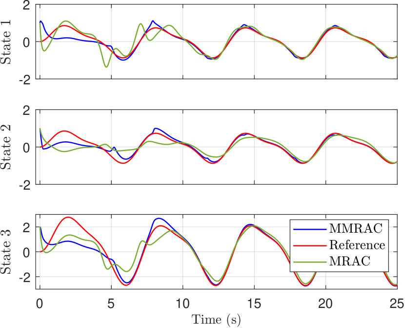
Figure 2: State of the system $x_{p}(t)$, and state of the reference model $x_{r}(t)$.

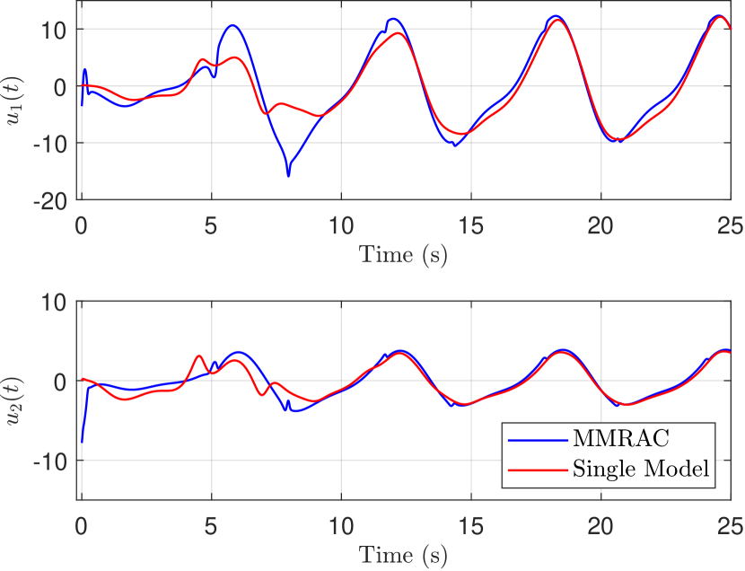
Figure 3: Control efforts for MMRAC and a single model MRAC.

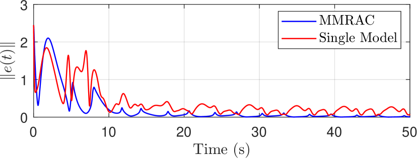
Figure 4: Euclidean norm of the tracking error for MMRAC and a single model MRAC.

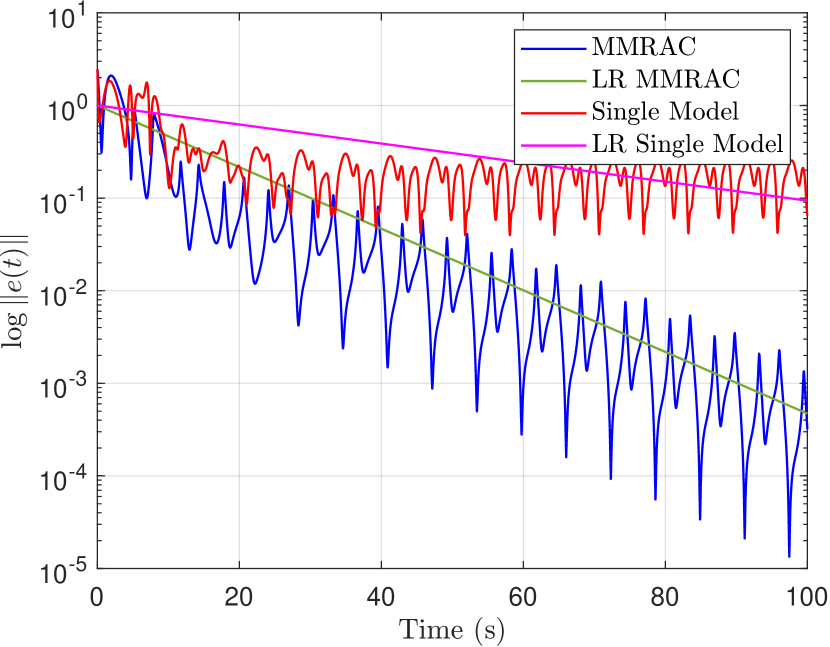
Figure 5: Semilog plot for the norm 2 of the tracking errors, and the linear regressions for MMRAC and a single model.

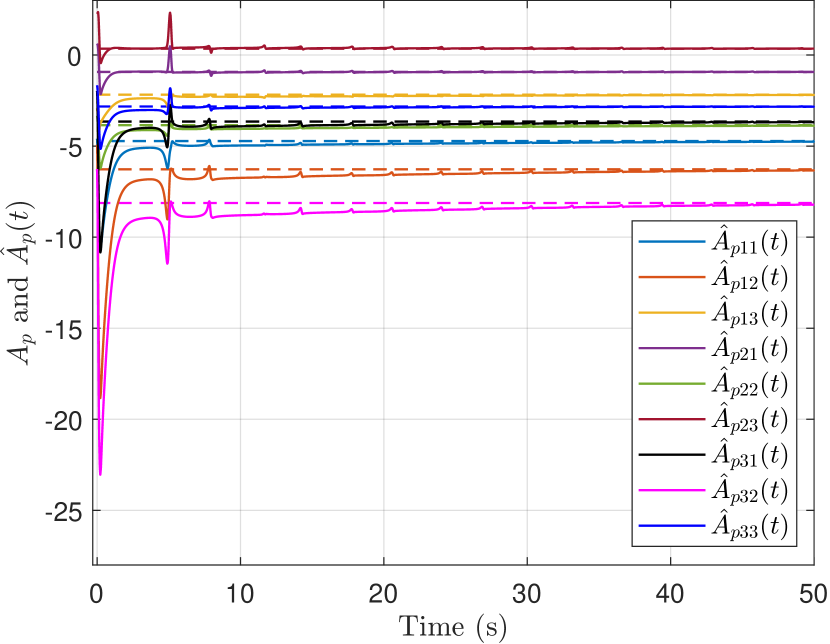
Figure 6: Estimation of each entry of $A_{p}$. The dashed line is the true value.

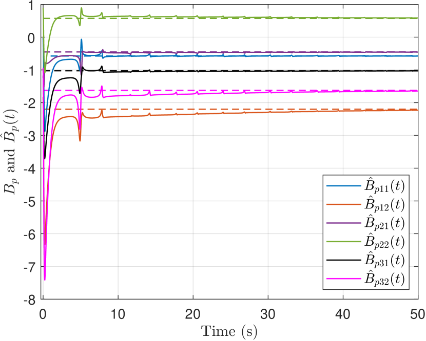
Figure 7: Estimation of each entry of $B_{p}$. The dashed line is the true value.

In this section, we illustrate the behavior and performance of the proposed MMRAC scheme through a set of simulation tests performed on an uncertain model (2), a reference model (3), and a set $\mathcal{S}$ (6) that defines the polytopic uncertainty. We compare the results with simulations using a single model for MRAC.

Consider the uncertain system with $n=3$, $m=2$ given by the matrices

$$A_{p}=\begin{bmatrix}-4.725&-6.275&-2.175\\ -0.925&-3.85&0.35\\ -3.65&-8.125&-2.825\end{bmatrix},\>B_{p}=\begin{bmatrix}-0.575&-2.2\\ -0.45&0.575\\ -1.025&-1.625\end{bmatrix}.$$

The reference model (3) is

$$A_{r}=\begin{bmatrix}-1&0&0\\ 0&-1&0\\ 1&1&-1\end{bmatrix},\>B_{r}=\begin{bmatrix}1&0\\ 0&1\\ 1&1\end{bmatrix}.$$

It can be verified that Assumption 1 is satisfied by defining the matrices

$$K^{*}=\begin{bmatrix}-3.16&-7.48&-0.36\\ -0.87&-0.89&-0.89\end{bmatrix},L^{*}=\begin{bmatrix}-0.44&-1.66\\ -0.34&0.44\end{bmatrix}.$$

Considering the following $5$ matrix pairs

$$A_{1}=\begin{bmatrix}-0.75&0.25&0.25\\ -3.75&-4.75&-3.75\\ -2.5&-2.5&-4.5\end{bmatrix},B_{1}=\begin{bmatrix}0.25&-0.5\\ 1.25&2.5\\ 1.5&2\end{bmatrix},$$

$$A_{2}=\begin{bmatrix}-16&-30&-5\\ -3.5&-8.5&-1.5\\ -17.5&-36.5&-7.5\end{bmatrix},B_{2}=\begin{bmatrix}-5&-10\\ -1&-2.5\\ -6&-12.5\end{bmatrix},$$

$$A_{3}=\begin{bmatrix}2&0&-1\\ -0.5&-1.5&-0.5\\ -0.5&0.5&-2.5\end{bmatrix},B_{3}=\begin{bmatrix}-1&1\\ -0.5&0\\ -1.5&1\end{bmatrix},$$

$$A_{4}=\begin{bmatrix}-1.5&-0.75&-0.75\\ -0.25&-0.875&1.125\\ 0.25&0.375&-0.625\end{bmatrix},B_{4}=\begin{bmatrix}0.25&0.25\\ 0.125&-0.375\\ 0.375&-0.125\end{bmatrix},$$

$$A_{5}=\begin{bmatrix}-4&-1&-5\\ 5&-2&8\\ 3&-1&2\end{bmatrix},B_{5}=\begin{bmatrix}2&-1\\ -3&2\\ -1&1\end{bmatrix},$$

we can define the set

$$\mathcal{S}=\left\{\begin{bmatrix}A_{1}&B_{1}\end{bmatrix},\cdots,\begin{bmatrix}A_{5}&B_{5}\end{bmatrix}\right\}.$$

The set $\mathcal{S}$ satisfies Assumption 2. The design parameters for the estimation scheme and the controller are $\Gamma=2I_{5\times 5}$, $\lambda=0.5$, and $\alpha=0.01$, with the initial condition $\hat{w}(0)=\begin{bmatrix}0.2&0.15&0.15&0.1&0.4\end{bmatrix}^{\top}$. The input to the reference model is taken to be $r_{1}\left(t\right)=r_{2}\left(t\right)=\sin{\left(t\right)}+0.5\sin{2t}$. With these definitions the full controller is

$$\begin{bmatrix}\dot{\phi}_{1}(t)\\ \dot{\phi}_{2}(t)\end{bmatrix} =-\lambda\begin{bmatrix}\phi_{1}(t)\\ \phi_{2}(t)\end{bmatrix}+\begin{bmatrix}x_{p}(t)\\ u(t)\end{bmatrix},$$

$$\dot{\hat{\bar{w}}}\left(t\right) =\operatorname{Pr}_{\Pi,\hat{\bar{w}}}\left(-\Gamma\left(E^{\top}\left(t\right)E\left(t\right)\hat{\bar{w}}\left(t\right)+E^{\top}\left(t\right)\varepsilon_{5}\left(t\right)\right)\right),$$

$$\hat{w}_{5}\left(t\right) =1-\sum_{i=1}^{4}\hat{w}_{i}\left(t\right),$$

$$\hat{K}\left(t\right) =\hat{B}_{p}^{\dagger}(t)\sum_{i=1}^{5}\hat{w}_{i}\left(t\right)B_{i}K_{i},$$

$$\hat{L}\left(t\right) =\hat{B}_{p}^{\dagger}(t)\sum_{i=1}^{5}\hat{w}_{i}\left(t\right)B_{i}L_{i},$$

$$u\left(t\right) =\hat{K}\left(t\right)x_{p}\left(t\right)+\hat{L}\left(t\right)r\left(t\right).$$

The simulations of the MMRAC are compared to a direct adaptive control technique using a single model MRAC (see Chapter 9 of [23]). The simulations consider the same initial condition for the system, the same reference, and the initial gains are calculated as

$$\hat{K}(0)=\hat{B}_{p}^{\dagger}(0)\sum_{i=0}^{5}w_{i}(0)K_{i},$$

$$\hat{L}(0)=\hat{B}_{p}^{\dagger}(0)\sum_{i=0}^{5}w_{i}(0)L_{i}.$$

In Figure 2 we see the time evolution of each of the states for the reference model, the states generated by the MMRAC, and the states generated by MRAC. Convergence is achieved for both controllers, with a clear advantage of the multiple-model technique while using approximately the same control effort, as depicted in Figure 3. The convergence speed is a key factor to consider, and there is a clear advantage of using multiple models when we analyze the dynamics of the error. In Figure 4 we compare the time evolution of the norm of the error for the case of MMRAC, and MRAC. To better visualize the advantage in convergence speed, we present the norm of the error in log-scale in Figure 5, as we perform a linear regression on each of the signals. We see that the convergence speed of the MMRAC scheme is approximately two order of magnitude faster than the single model approach (the slope of the linear regressions are -0.0333 and -0.0103 for MMRAC and a single model, respectively), matching with the conjecture in [29]. Finally, as mentioned in Section IV, we achieve asymptotic convergence of the estimated system’s matrices. In Figures 6 and 7 we see the asymptotic convergence of each entry of the matrix pairs $\begin{bmatrix}\hat{A}_{p}(t)&\hat{B}_{p}(t)\end{bmatrix}$ to $\begin{bmatrix}A_{p}&B_{p}\end{bmatrix}$, respectively.

VII Conclusions

In this article we developed a multiple model reference adaptive control (MMRAC) scheme for multi-input, linear, time-invariant systems with uncertain parameters that lie inside a known compact and convex polytope. The controller performs online parameter identification of the system matrices as a convex combination of an arbitrary number of fixed model, one at each extreme point of the convex polytope of uncertainty. The identification is proven to be asymptotically stable, and sufficient conditions for perfect identification of the uncertain system matrices are provided. The tracking controller of the MMRAC guarantees that all close-loop signals are bounded, and that the difference between the plant states and the ones generated by a linear reference model asymptotically converge to zero. To verify the effectiveness of the proposed MMRAC scheme we compare it to a single model MRAC scheme through MATLAB and Simulink simulations. For the simulation examples, we observe that the convergence speed is approximately two orders of magnitude faster than using a single model, with similar control effort. Future lines of research include generalizing the proposed scheme to linear, time-varying systems and nonlinear systems.

References

• [1] K. S. Narendra and Z. Han, “A new approach to adaptive control using multiple models,” International Journal of Adaptive Control and Signal Processing, vol. 26, no. 8, pp. 778–799, Aug. 2012.
• [2] A. S. Morse, “A simple example of an adaptive control system,” Communications in Information and Systems, vol. 11, no. 2, pp. 105–118, 2011.
• [3] M. Kuipers and P. Ioannou, “Multiple model adaptive control with mixing,” IEEE Transactions on Automatic Control, vol. 55, no. 8, pp. 1822–1836, Aug. 2010.
• [4] J. P. Hespanha, D. Liberzon, and A. S. Morse, “Overcoming the limitations of adaptive control by means of logic-based switching,” Systems & Control Letters, vol. 49, no. 1, pp. 49–65, May 2003.
• [5] G. M. Prasad, V. Kedia, and A. S. Rao, “Multi-model predictive control (mmpc) for non-linear systems with time delay: An experimental investigation,” in IEEE International Conference on Measurement, Instrumentation, Control and Automation, 2020, pp. 1–5.
• [6] L. Vu and D. Liberzon, “Supervisory control of uncertain linear time-varying systems,” IEEE Transactions on Automatic Control, vol. 56, no. 1, pp. 27–42, 2011.
• [7] J. P. Hespanha and A. S. Morse, “Switching between stabilizing controllers,” Automatica, vol. 38, no. 11, pp. 1905–1917, Nov. 2002.
• [8] J. P. Hespanha, D. Liberzon, A. S. Morse, B. D. O. Anderson, T. S. Brinsmead, and F. De Bruyne, “Multiple model adaptive control. Part 2: switching,” International Journal of Robust and Nonlinear Control, vol. 11, no. 5, pp. 479–496, Apr. 2001.
• [9] H. Zengin, N. Zengin, B. Fidan, and A. Khajepour, “Blending based multiple-model adaptive control of multivariable systems with application to lateral vehicle motion control,” European Journal of Control, vol. 58, pp. 1–10, Mar. 2021.
• [10] K. Büyükkabasakal, B. Fidan, and A. Savran, “Mixing adaptive fault tolerant control of quadrotor UAV,” Asian Journal of Control, vol. 19, no. 4, pp. 1441–1454, Jul. 2017.
• [11] J. L. Mancilla-Aguilar and R. A. García, “An algorithm for the robust exponential stabilization of a class of switched systems,” International Journal of Robust and Nonlinear Control, vol. 25, no. 13, pp. 2062–2082, Sep. 2015.
• [12] G. Evensen, Data Assimilation: The Ensemble Kalman Filter, 2nd ed.   Berlin, Heidelberg: Springer-Verlag, 2009.
• [13] A. Dehghani, B. D. O. Anderson, and A. Lanzon, “Unfalsified adaptive control: A new controller implementation and some remarks,” in IEEE European Control Conference, 2007, pp. 709–716.
• [14] S. Baldi, G. Battistelli, E. Mosca, and P. Tesi, “Multi-model unfalsified adaptive switching supervisory control,” Automatica, vol. 46, no. 2, pp. 249–259, 2010.
• [15] K. S. Narendra and K. Esfandiari, “Adaptive identification and control of linear periodic systems using second-level adaptation,” International Journal of Adaptive Control and Signal Processing, vol. 33, no. 6, pp. 956–971, Jun. 2019.
• [16] Y. Zhang, X. Wang, and Z. Wang, “Adaptive multiple model control for a class of nonlinear discrete time systems: second-level adaption design approach,” International Journal of Control, vol. 96, no. 2, pp. 497–507, 2023.
• [17] V. K. Pandey, I. Kar, and C. Mahanta, “Controller design for a class of nonlinear mimo coupled system using multiple models and second level adaptation,” ISA Transactions, vol. 69, pp. 256–272, 2017.
• [18] L. Dutta and D. Kumar D., “Adaptive model predictive control design using multiple model second level adaptation for parameter estimation of two‐degree freedom of helicopter model,” International Journal of Robust and Nonlinear Control, vol. 31, no. 8, pp. 3248–3278, 2021.
• [19] K. Moffat and C. Tomlin, “The Multiple Model Adaptive Power System State Estimator,” in IEEE Conference on Decision and Control, Dec. 2021, pp. 3525–3530.
• [20] M. Imani and U. Braga-Neto, “Multiple Model Adaptive controller for Partially-Observed Boolean Dynamical Systems,” in American Control Conference, May 2017, pp. 1103–1108.
• [21] S. Wang, W. Ren, and J. Chen, “Fully distributed state estimation with multiple model approach,” in IEEE Conference on Decision and Control, Dec. 2016, pp. 2920–2925.
• [22] P. Ioannou and B. Fidan, Adaptive Control Tutorial.   SIAM, 2006.
• [23] G. Tao, Adaptive Control Design and Analysis.   Wiley, 2003.
• [24] Z. Han and K. S. Narendra, “New concepts in adaptive control using multiple models,” IEEE Transactions on Automatic Control, vol. 57, no. 1, pp. 78–89, Jan. 2012.
• [25] N. Ahmadian, A. Khosravi, and P. Sarhadi, “A New Approach to Adaptive Control of Multi-Input Multi-Output Systems Using Multiple Models,” ASME Journal of Dynamic Systems, Measurement, and Control, vol. 137, no. 9, p. 091009, Sep. 2015.
• [26] A. Lovi, B. Fidan, and C. Nielsen, “Multiple model reference adaptive tracking control of multivariable systems with blending,” in IEEE Conference on Decision and Control, 2022, pp. 1362–1367.
• [27] B. Kolodziejczak and T. Szulc, “Convex combinations of matrices — full rank characterization,” Linear Algebra and its Applications, vol. 287, no. 1-3, pp. 215–222, 1999.
• [28] S. P. Boyd and L. Vandenberghe, Convex Optimization, 2nd ed.   Cambridge, UK: Cambridge University Press, 2006.
• [29] K. S. Narendra, W. Yu, and C. Wei, “Stability, robustness, and performance issues in second level adaptation,” in American Control Conference, 2014, pp. 2377–2382.