Assessing COVID-19 vaccine effectiveness in observational studies via nested trial emulation

Abstract

Observational data are often used to estimate real-world effectiveness and durability of coronavirus disease 2019 (COVID-19) vaccines. A sequence of nested trials can be emulated to draw inference from such data while minimizing selection bias, immortal time bias, and confounding. Typically, when nested trial emulation (NTE) is employed, effect estimates are pooled across trials to increase statistical efficiency. However, such pooled estimates may lack a clear interpretation when the treatment effect is heterogeneous across trials. In the context of COVID-19, vaccine effectiveness quite plausibly will vary over calendar time due to newly emerging variants of the virus. This manuscript considers a NTE inverse probability weighted estimator of vaccine effectiveness that may vary over calendar time, time since vaccination, or both. Statistical testing of the trial effect homogeneity assumption is considered. Simulation studies are presented examining the finite-sample performance of these methods under a variety of scenarios. The methods are used to estimate vaccine effectiveness against COVID-19 outcomes using observational data on over 120,000 residents of Abruzzo, Italy during 2021.

Keywords Causal inference  $\cdot$ COVID-19  $\cdot$ Nested trial emulation  $\cdot$ Observational studies  $\cdot$ Vaccine effectiveness

1 Introduction

As of March 3, 2024, over 774 million cases of coronavirus disease 2019 (COVID-19) have been confirmed worldwide (World Health Organization, 2024). COVID-19 vaccines were developed with unprecedented speed and remain critical to pandemic containment efforts. Randomized controlled trials found high efficacy of Pfizer-BioNTech, Moderna, Oxford-AstraZeneca, and Janssen vaccines against moderate-to-severe COVID-19 (Polack et al., 2021; Baden et al., 2021; Falsey et al., 2021; Sadoff et al., 2021). In many parts of the world, COVID-19 vaccines were initially deployed in late 2020 and are now widely available.

To estimate effectiveness and durability of COVID-19 vaccines in a real-world setting, observational data are needed. One important goal is to determine whether protection offered by COVID-19 vaccines wanes over time since vaccination, across calendar time (as new variants of the SARS-CoV-2 virus emerge), or both (Lin et al., 2022). Ideally, this question could be addressed by conducting a series of randomized trials, where each trial is initiated at a different calendar date, and estimating the vaccine effect separately for each trial. However, since such an approach is generally not feasible, vaccine effectiveness (VE) studies must rely on observational data.

Target trial emulation is one approach for drawing inference from observational data while avoiding biases that can arise in observational analyses (Hernán and Robins, 2016; Hernán et al., 2016). The first step in a target trial emulation analysis entails developing a protocol for a hypothetical randomized trial designed to address a specific causal question. Important components of the target trial protocol include eligibility criteria, the treatment regimens to be compared, and definition of “time zero" (the date when follow up begins). Then, the observational database is prepared and analyzed to emulate each component of the hypothetical (target) trial. When some individuals in the observational database meet eligibility criteria at multiple time points, nested trial emulation (NTE; Hernán, Robins, and Garcia Rodríguez, 2005) can be used to properly align time zero. That is, a sequence of nested trials are emulated, with time zero of each trial corresponding to the calendar time point at which eligibility can be determined. A key feature of NTE is that each individual in the database is “enrolled” in all emulated trials for which they are eligible. NTE has recently been applied to estimate COVID-19 VE from large observational databases (McConeghy et al., 2022; Gazit et al., 2023).

Often when NTE is used, treatment effect estimates are pooled across the emulated trials to increase statistical efficiency (e.g., Hernán et al., 2008; Danaei et al., 2013, 2018). Such pooled estimates may lack a clear interpretation when the treatment effect is heterogeneous across trials. The assumption of trial effect homogeneity (TEH) may be plausible in some contexts, e.g., if the goal is to estimate the effect of statin initiation on prevention of coronary heart disease (Danaei et al., 2013). However, COVID-19 VE may vary across trials due to calendar-time-specific factors like newly emerging viral strains and pandemic control policies. The TEH assumption can be assessed using a formal hypothesis test (Hernán et al., 2008; Keogh et al., 2023). Moreover, assessing potential heterogeneity in VE over calendar time (i.e., across trials) may itself be of scientific interest. NTE is particularly well suited for this task, as trial-specific VE estimates can be used to discern patterns of waning vaccine protection across calendar time as well as time since vaccination.

This manuscript uses a NTE approach to estimate VE over both time scales and to test the TEH assumption. Section 2 describes the problem setup and inference procedures. Methods are demonstrated in Section 3 through simulation studies. In Section 4, methods are applied to estimate COVID-19 VE using a large database of Abruzzo, Italy residents (Acuti Martellucci et al., 2022). Section 5 concludes with a discussion. The Supporting Information contains additional methodological details, additional simulation results, and the target trial protocol for the application.

2 Methods

2.1 Target estimand

Suppose the goal is to estimate VE against a COVID-19 outcome (e.g., SARS-CoV-2 infection, COVID-19-related hospitalization or death), allowing for the possibility that VE varies over calendar time, time since vaccination, or both. Ideally, a series of randomized controlled trials could be conducted, each initiated from a different calendar date, and VE could be estimated separately for each trial. For this ideal scenario, let $j=0,1,...,J$ denote trial number, ordered by calendar date of initiation. At the start of each trial, eligibility would be assessed and participants would be randomly assigned to receive an active vaccine regimen, denoted $Z=1$, or a comparator regimen, denoted $Z=0$. Assume in this ideal setting that all participants fully adhere to their assigned regimen. Individuals would be assessed for a COVID-19 event of interest at a series of evenly-spaced follow-up visits. Assume weekly follow-up visits and let $k$ index time in weeks since the start of a given trial.

The VE estimand can be defined using potential outcomes. Let $Y^{z}_{j}(k)$ denote a binary potential outcome for a COVID-19 event by time $k$ of trial $j$ under treatment regimen $z$. The target estimand is

$$VE_{j}(k)=1-\frac{P\{Y_{j}^{1}(k)=1\}}{P\{Y_{j}^{0}(k)=1\}}$$ (1)

for $j=0,1,...,J$ and $k$ varying over a specified range of follow-up times. The ratio $P\{Y_{j}^{1}(k)=1\}/P\{Y_{j}^{0}(k)=1\}$ is a causal contrast comparing the counterfactual risk at time $k$ of trial $j$ under regimens $Z=1$ and $Z=0$. Variation in $VE_{j}(k)$ over $j$ indicates the vaccine’s effect is changing over calendar time, whereas variation in $VE_{j}(k)$ over $k$ conveys the vaccine effect changes with time since vaccination. Alternatively, $VE_{j}(k)$ could be defined as one minus the hazard ratio at time $k$ in trial $j$ (Halloran, Longini, and Struchiner, 2010). Given issues that arise in the causal interpretation of hazard ratios (Hernán, 2010; Aalen, Cook, and Røysland, 2015; Martinussen, Vansteelandt, and Andersen, 2020), the developments in this manuscript focus on the risk ratio VE estimand (1).

Since conducting a series of randomized trials is unlikely to be feasible, observational data can be used to emulate the desired series of trials. This manuscript aims to draw inference about (1) from observational data via NTE. Throughout the remainder of Section 2, methods are developed in the context of the Abruzzo study analyzed in Section 4.

2.2 The Abruzzo study

The Abruzzo COVID-19 VE study (Acuti Martellucci et al., 2022) utilized individual data available from the Italian National Health Service on medical and demographic characteristics and COVID-19 vaccination status and outcomes. The study included all persons residing or domiciled in the Abruzzo region of Italy on January 1, 2020 and without a positive SARS-CoV-2 swab prior to January 2, 2021 ($N=1,279,694$). Baseline characteristics (age, sex, risk factors/comorbidities) were known for all individuals. The database includes COVID-19 vaccination date and type (either Pfizer-BioNTech, Moderna, Oxford-AstraZeneca, or Janssen) for each dose received between January 2, 2021 and December 18, 2021 (up to three doses per individual). Calendar date for each of the following was recorded between January 2, 2021 and February 18, 2022: first SARS-CoV-2 infection (positive reverse transcription polymerase chain reaction test from an accredited laboratory in Abruzzo), first severe COVID-19 disease (requiring hospitalization), and death (with or without positive SARS-CoV-2 swab).

2.3 Emulating target trials using observational data

2.3.1 Analytic cohort

Suppose there is interest in applying NTE to estimate COVID-19 VE during 2021 using the Abruzzo study data. Consider a sequence of emulated trials initiated weekly from Feb 15, 2021 to May 3, 2021, with each trial ending on Dec 18, 2021. Let $l=0,1,...,\tau$ index calendar time, measured in weeks from February 15, where $l=J$ corresponds to the week of May 3 and $\tau=44$ is the administrative censoring time.

This section describes how specifications in the target trial protocol for the application in Section 4 are used to construct an analytic cohort from the Abruzzo data; the full protocol appears in Table A.1. Individuals are “enrolled" into all trials for which they are eligible. Assume people enter the analytic cohort on the first full week during which they meet eligibility criteria. Further assume eligibility criteria are defined such that a person may be eligible for one or more consecutive trials, but a person who is ineligible for the week-$l$ trial will also be ineligible for all subsequent trials. Define the analytic cohort as the set of all individuals in the Abruzzo study database who are alive and free of the event on February 15, 2021 and meet eligibility criteria for at least one trial.

Assume a “study visit" (data collection time) occurs on the first day of each week during the follow-up period. Time-dependent variables are measured in weeks and determined by changes in a participant’s status between study visits. Let $T$ denote calendar time of the event of interest, measured in weeks from $l=0$ (i.e., February 15, 2021). Similarly, let $C$ denote calendar time of censoring (due to loss to follow up, as defined in the target trial protocol). Let $T^{*}=\text{min}(T,C)$ and $\Delta=I(T<C)$, where $I(\cdot)$ denotes the indicator function. For example, if an individual experiences an event on or after the day of the week $l-1$ visit and before the day of the week $l$ visit, then $T^{*}=l$ and $\Delta=1$. If an individual remains free of the event and censoring by the administrative censoring time $\tau$, then $\Delta=0$ and $C=\tau+1$. Let $S$ and $S^{*}$ denote the first and last calendar time when eligibility criteria are met, respectively, such that $S^{*}\in\{S,S+1,...,J\}$. Let $\boldsymbol{V}=(V_{1},V_{2},V_{3})$ where $V_{q}$ represents calendar time of the $q$th COVID-19 vaccine dose. By convention, let $V_{q}=\infty$ if an individual is lost to follow up or experiences an event prior to receiving a $q$th vaccine dose. Let $\boldsymbol{X}$ denote a vector of time-fixed covariates measured prior to calendar time $l=0$. Assume independent and identically distributed copies of $\boldsymbol{O}=(T^{*},\Delta,S,S^{*},\boldsymbol{V},\boldsymbol{X})$ are observed for the $n$ individuals in the analytic cohort.

2.3.2 The emulated trials

For each emulated trial $j\in\{0,1,...,J\}$, the follow-up period coincides with calendar times $j,j+1,...,\tau$. Recall that time in weeks since the start of a given trial is indexed by $k$. For trial $j$, let $K_{j}=\tau-j$ denote the duration of follow up (in weeks) and note that time $k$ occurs at calendar time $j+k$. Let $\mathcal{W}=\{(j,k)\subset\mathbb{Z}^{+}_{0}\times\mathbb{Z}^{+}_{0}:0\leq j\leq J,$ $0\leq k\leq K_{j}\}$ denote the set of all time points in the NTE study period, where $\mathbb{Z}^{+}_{0}$ represents the non-negative integers.

Observed data are used to “assign" eligible individuals to a vaccine regimen in each trial, according to specifications in the target trial protocol. Consider vaccine regimens $Z=0$ “remain unvaccinated through December 18, 2021" and $Z=1$ “receive a first COVID-19 vaccine dose within one to seven days of trial enrollment, receive a second dose within six weeks of the initial dose, and receive no further COVID-19 vaccine doses through December 18, 2021." Assume prior uptake of the vaccine is among the exclusion criteria. Therefore, individuals assigned to regimen $Z=0$ in trial $j$ may be enrolled in trials $j+1,j+2,...,J$, provided they continue to meet other eligibility criteria, but those assigned to $Z=1$ in trial $j$ are ineligible for subsequent trials. Recall that $V_{1}=l+1$ if an individual receives a first vaccine dose during calendar week $l$. Thus, if a person with $V_{1}=j+1$ is eligible for trial $j$, they are enrolled in trial $j$ with regimen assignment $Z=1$ and excluded from all subsequent trials. Let $Z_{j}=I(V_{1}\leq j+1)$ be an indicator for uptake of regimen $Z=1$ by calendar time $j$.

For example, consider a hypothetical individual with observed data $O=(T^{*}=4,\Delta=1,S=0,S^{*}=2,\boldsymbol{X}=\boldsymbol{x},\boldsymbol{V}=(3,\infty,\infty))$. Thus, $(Z_{0},Z_{1},Z_{2})=(0,0,1)$, i.e., the individual is enrolled in trial $0$ with regimen assignment $Z=0$, trial $1$ with $Z=0$, and trial $2$ with $Z=1$. After receiving a first vaccine dose, the individual is ineligible for subsequent trials (i.e., trials $3,4,...,J$). Figure 1 illustrates the hypothetical individual’s contribution to trials 0, 1, and 2.

Methods in this manuscript aim to estimate the observational analogue of a per-protocol effect, i.e., VE corresponding to perfect adherence to the active vaccine regimen. An individual’s trial $j$ record is censored if the individual (i) no longer follows their trial-$j$ regimen assignment, (ii) is lost to follow-up, or (iii) reaches the administrative censoring time $K_{j}$ (on the trial time scale) without experiencing (i), (ii), or an event. Let $R_{j}(k)$ be a binary indicator for remaining uncensored at time $k$ in trial $j$. Specifically, if an individual is eligible for trial $j$, $R_{j}(k)$=$1-\text{max}\{I(Z_{j}=0,V_{1}\leq j+k+1)$, $I(Z_{j}=1,k\geq 6,V_{2}-V_{1}>6)$, $I(Z_{j}=1,V_{3}\leq j+k)$, $I(T^{*}\leq j+k,\Delta=0)\}$ for all $k\in\{0,1,...,K_{j}\}$; otherwise $R_{j}(k)$ is undefined. For example, the hypothetical individual described above receives a first COVID-19 vaccine during the interval March 1-7, 2021, so $V_{1}=3$. Their trial 1 record is artificially censored (Robins and Finkelstein, 2000) when they initiate the active regimen, i.e., $R_{1}(k)=1-I(Z_{1}=0,V_{1}\leq 2+k)=0$ for all $k\in\{1,2,...,K_{1}\}$.

Let $Y_{j}(k)$ be the indicator of an observed event by time $k$ of trial $j$. Specifically, if an individual is eligible for trial $j$, then $Y_{j}(k)=I(T^{*}\leq j+k,\Delta=1)$ for all $k\in\{0,1,...,K_{j}\}$; otherwise $Y_{j}(k)$ is undefined. An individual is at risk of having an observed event at time $k$ of trial $j$ if $R_{j}(k-1)=1$ and $Y_{j}(k-1)=0$. In the running example, the hypothetical participant experienced a COVID-19 hospitalization just prior to the week $l=T^{*}\Delta=4$ visit (see Figure 1). Their trial $2$ record was at risk (because $R_{2}(1)=1$ and $Y_{2}(1)=0$), so they contribute an event to the analysis at time $k=2$ of trial $j=2$, i.e., $Y_{2}(2)=I(T^{*}\leq 4,\Delta=1)=1$. However, their trial $0$ and $1$ records (red lines in Figure 1) were not at risk when the event occurred (because $R_{0}(3)=R_{1}(2)=0$), so they do not contribute events to the analysis for trials $0$ and $1$.

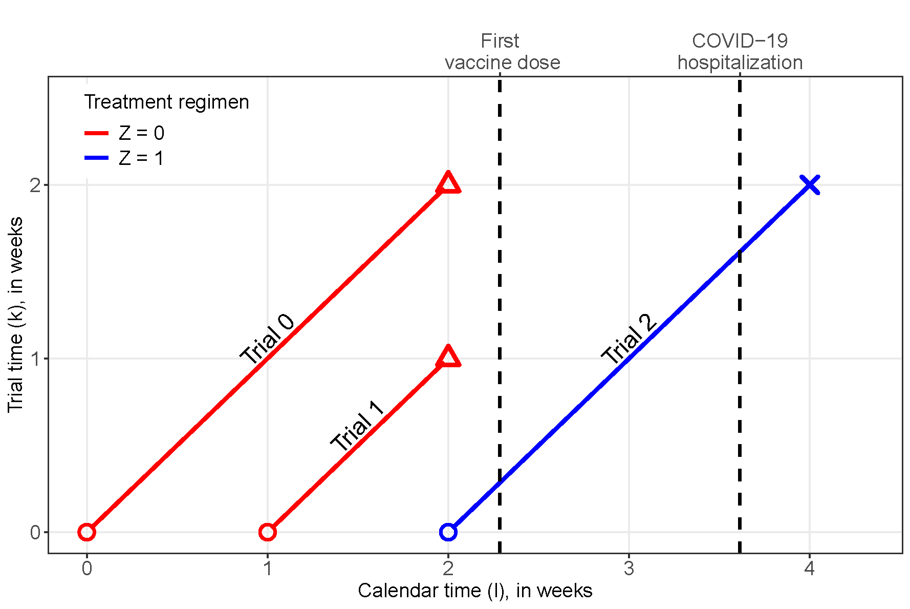
Figure 1: Lexis diagram illustrating trial-specific data for a hypothetical individual with observed data $\{T^{*}=4,\Delta=1,S=0,S^{*}=2,\boldsymbol{X}=\boldsymbol{x},\boldsymbol{V}=(3,\infty,\infty)\}$. Circles represent entry into trial-specific cohorts, diagonal lines time spent at risk, triangles censoring, and the cross an event. This individual is “enrolled” in trial 0 in treatment group $Z_{0}=0$, trial 1 in group $Z_{1}=0$, and trial 2 in group $Z_{2}=1$. They are ineligible for subsequent trials. Trial-specific variables are derived using calendar time (horizontal axis) and trial time (vertical axis). For example, the trial 0 record is censored at trial time $k=2$, such that $R_{0}(2)=0$, because the individual ceases to follow their “assigned" trial 0 regimen at calendar time $l=2$. Similarly, the trial 1 record is censored at trial time $k=1$, so that $R_{1}(1)=0$. The trial 2 record has an event at trial time $k=2$, such that $Y_{2}(2)=1$, since the individual experiences a COVID-19 hospitalization in the week prior to calendar time $l=4$.

2.4 Potential outcomes and identifiability assumptions

Let $T^{v_{1}}$ denote potential (or counterfactual) calendar time of the event under the treatment strategy “initiate vaccine regimen $Z=1$ at calendar time $v_{1}-1$ and remain adherent to that strategy through December 18, 2021". Similarly, let $T^{v_{1}>\tau}$ denote potential calendar time of the event under the treatment strategy “refrain from initiating $Z=1$ through December 18, 2021". An individual who enters the analytic cohort at calendar time $s$ and continues to meet eligibility criteria through calendar time $s^{*}$ is assumed to have the following set of $s^{*}-s+2$ potential outcomes: $\{T^{v_{1}=s+1}$, $T^{v_{1}=s+2}$, $...$, $T^{v_{1}=s^{*}}$, $T^{v_{1}=s^{*}+1}$, $T^{v_{1}>\tau}\}$. Potential outcomes can be re-expressed in the emulated trial notation. Recall that $Y_{j}^{z}(k)$ represents a binary potential outcome for an event by time $k$ of trial $j$ under adherence to vaccine regimen $Z=z$ for $z\in\{0,1\}$. Assume the following for all $(j,k)\in\mathcal{W}$: $Y_{j}^{1}(k)=I(T^{v_{1}=j+1}\leq j+k)$ if $T^{v_{1}=j+1}\geq j$, $Y_{j}^{1}(k)$ is undefined otherwise, $Y_{j}^{0}(k)=I(T^{v_{1}>\tau}\leq j+k)$ if $T^{v_{1}>\tau}\geq j$, and $Y_{j}^{0}(k)$ is undefined otherwise.

The following conventions and assumptions are adopted for the remainder of the manuscript. Vectors are bolded and are assumed to be row vectors except where noted otherwise. Let $\boldsymbol{X_{1}}\subset\boldsymbol{X}$ and $\boldsymbol{X_{2}}\subset\boldsymbol{X}$ denote possibly overlapping covariate vectors, and let $e_{j}(\boldsymbol{\boldsymbol{X_{1}}})$=$P\{Z_{j}=1\mid R_{j}(0)=1,\boldsymbol{X_{1}}\}$ denote the trial-$j$ propensity score. Noting that, when an individual is eligible for trial $j$, their treatment regimen “assignment" is equal to $Z_{j}$, let $d_{jk}({Z_{j}}$, $\boldsymbol{X_{2}})$=$P\{R_{j}(k)=1\mid R_{j}(k-1)=1$, $Y_{j}(k-1)=0$, $Z_{j}$, $\boldsymbol{X_{2}}\}$ denote the hazard of remaining uncensored at time $k$ of trial $j$, conditional on vaccine regimen assignment in trial $j$ and covariates. Assume that all variables are measured without error, and assume the following for all $(j,k)\in\mathcal{W}$ and $z\in\{0,1\}$: $Y_{j}^{z}(k)\mathchoice{\mathrel{\hbox to0.0pt{$\displaystyle\perp$\hss}\mkern 2.0mu{\displaystyle\perp}}}{\mathrel{\hbox to0.0pt{$\textstyle\perp$\hss}\mkern 2.0mu{\textstyle\perp}}}{\mathrel{\hbox to0.0pt{$\scriptstyle\perp$\hss}\mkern 2.0mu{\scriptstyle\perp}}}{\mathrel{\hbox to0.0pt{$\scriptscriptstyle\perp$\hss}\mkern 2.0mu{\scriptscriptstyle\perp}}}Z_{j}\mid\{\boldsymbol{X_{1}},R_{j}(0)=1\}$ (conditional exchangeability); $Y_{j}^{z}(k^{\prime})\mathchoice{\mathrel{\hbox to0.0pt{$\displaystyle\perp$\hss}\mkern 2.0mu{\displaystyle\perp}}}{\mathrel{\hbox to0.0pt{$\textstyle\perp$\hss}\mkern 2.0mu{\textstyle\perp}}}{\mathrel{\hbox to0.0pt{$\scriptstyle\perp$\hss}\mkern 2.0mu{\scriptstyle\perp}}}{\mathrel{\hbox to0.0pt{$\scriptscriptstyle\perp$\hss}\mkern 2.0mu{\scriptscriptstyle\perp}}}R_{j}(k)\mid\{{Z_{j}=z},\boldsymbol{X_{2}},R_{j}(k-1)=1$, $Y_{j}(k-1)=0\}$ for all integers $k^{\prime}$ such that $k\leq k^{\prime}\leq K_{j}$ (ignorable censoring); if $f_{\boldsymbol{X_{1}},R_{j}(0)}(\boldsymbol{x_{1}},1)>0$, then $0<e_{j}(\boldsymbol{X_{1}})<1$ and if $f_{\boldsymbol{X_{2}},Z_{j},R_{j}(k-1),Y_{j}(k-1)}(\boldsymbol{x_{2}},z,1,0)>0$, then $d_{jk}(Z_{j},\boldsymbol{X_{2}})>0$, where in general $f_{\boldsymbol{A}}$ denotes the cumulative distribution function of random variable $\boldsymbol{A}$ (positivity); an individual’s potential outcomes $Y_{j}^{z}(k)$ are unaffected by whether another individual follows regimen $z=0$ or $z=1$ in trial $j^{\prime}$ for all $j^{\prime}\in\{0,1,...,J\}$ (no interference between individuals; Cox, 1958); and if $R_{j}(k)=1$, then $Y_{j}(k)=(1-Z_{j})Y^{0}_{j}(k)+Z_{j}Y^{1}_{j}(k)$ (causal consistency).

2.5 Inverse probability weighted VE estimator

Observe that (1) can be re-expressed as

$${VE}_{j}(k)=1-\dfrac{1-\prod_{m=1}^{k}\{1-{\lambda}_{j}^{1}(m)\}}{1-\prod_{m=1}^{k}\{1-{\lambda}_{j}^{0}(m)\}},$$ (2)

where $\lambda_{j}^{z}(k)=P\{Y_{j}^{z}(k)=1$ $\mid Y_{j}^{z}(k-1)=0\}$ is the counterfactual (discrete time) hazard of the outcome at time $k$ of trial $j$ under vaccine regimen $z$. Following Hernán and Robins (2020, Ch. 17), Section 2.5.2 describes a plug-in VE estimator based on (2). Specifically, inverse probability weighted estimators of the counterfactual hazards are proposed based on an assumed marginal structural model (MSM) which allows the outcome hazard to depend on calendar time, time since vaccination, or both. The following section compares several MSM specifications.

2.5.1 Modeling framework

Consider the MSM

$$\text{logit}\{\lambda_{j}^{z}(k)\}=\alpha_{0}+\alpha_{1}z+\boldsymbol{\alpha_{2}}\boldsymbol{f_{1}}(k)z+\boldsymbol{\alpha_{3}}\boldsymbol{f_{2}}(j+k)+\boldsymbol{\alpha_{4}}\boldsymbol{f_{3}}(j+k)z,$$ (3)

where $\boldsymbol{f_{1}}(\cdot)$, $\boldsymbol{f_{2}}(\cdot)$, and $\boldsymbol{f_{3}}(\cdot)$ are column vectors of user-specified functions. According to (3), if $\boldsymbol{\alpha_{2}}\neq\boldsymbol{0}$ and at least one of $\boldsymbol{\alpha_{3}}$ or $\boldsymbol{\alpha_{4}}$ is non-zero, then the counterfactual hazard under $z=1$ will in general vary over both calendar time and time since vaccination. Since the hazard for the outcome when unvaccinated should not depend on time since “enrollment" in a hypothetical trial, the counterfactual hazard under $z=0$ is assumed under model (3) to be a one-dimensional function of calendar time $j+k$. Thus, the hazard under $z=0$ at a fixed calendar time, say $j+k=3$, is the same regardless of trial number, i.e., $\lambda_{0}^{0}(3)=\lambda_{1}^{0}(2)=\lambda_{2}^{0}(1)=\text{logit}^{-1}\{\alpha_{0}+\boldsymbol{\alpha_{3}}\boldsymbol{f_{2}}(3)\}$. The expression $\alpha_{0}+\boldsymbol{\alpha_{3}}\boldsymbol{f_{2}}(j+k)$ can be interpreted as a calendar-time-varying intercept representing the logit hazard when unvaccinated at calendar time $j+k$; $\alpha_{1}+\boldsymbol{\alpha_{4}}\boldsymbol{f_{3}}(j+k)$ captures the change to the logit hazard at calendar time $j+k$ if vaccinated; and $\boldsymbol{\alpha_{2}}\boldsymbol{f_{1}}(k)$ represents the change to the logit hazard $k$ weeks after vaccination.

As an alternative to (3), one could consider more general MSMs. For example, the outcome hazard could be modeled separately for each trial so that

$$\text{logit}\{\lambda_{j}^{z}(k)\}=\alpha_{0}+\alpha_{1j}z+\boldsymbol{\alpha_{2j}}\boldsymbol{f_{1}}(k)z+\boldsymbol{\alpha_{3}}\boldsymbol{f_{2}}(j+k),$$ (4)

where $\alpha_{1j}+\boldsymbol{\alpha_{2j}}\boldsymbol{f_{1}}(k)$ represents the change to the hazard when vaccinated at time $k$ of trial $j$. Here, as in model (3), the hazard when unvaccinated is assumed to be a one-dimensional function of calendar time. Note that the modeling approach in (3) “borrows" information across trials to estimate the hazard trajectory under vaccination over both time scales. However, (3) assumes that the increment to the logit hazard when vaccinated can be decomposed into additive calendar time and time since vaccination effects. Adopting model (4) would circumvent this assumption, although the dimension of the nuisance parameters under (4) may become unwieldy when emulating more than a few trials.

In some infectious disease settings (e.g., measles), MSMs that are more restrictive than (3) may be appropriate. For example, the antigenic profile of measles virus is stable across calendar time. In turn, measles vaccines that were developed decades ago offer protection against measles viruses in circulation today (Tahara et al., 2016; Zemella et al., 2024). In such a setting, one might posit the MSM

$$\text{logit}\{\lambda_{j}^{z}(k)\}=\alpha_{0}+\alpha_{1}z+\boldsymbol{\alpha_{2}}\boldsymbol{f_{1}}(k)z+\boldsymbol{\alpha_{3}}\boldsymbol{f_{2}}(j+k)$$ (5)

which is a special case of (3) with $\boldsymbol{\alpha_{4}}=\boldsymbol{0}$. Under the stronger assumption that hazards under both $z=0$ and $z=1$ do not depend on calendar time, but the hazard under $z=1$ may depend on time since vaccination, an even more restrictive version of (3) with $\boldsymbol{\alpha_{3}}=\boldsymbol{\alpha_{4}}=\boldsymbol{0}$ could be considered.

By contrast, the SARS-CoV-2 virus mutates rapidly, leading to emergence of new variants. Current COVID-19 vaccines are designed to elicit an immune response to specific SARS-CoV-2 antigens and, in turn, may not protect against COVID-19 disease given exposure to a SARS-CoV-2 variant with a different antigenic structure. Therefore, the application in Section 4 utilizes models of the form (3) that allow for changes in the hazard when vaccinated across calendar time and time since vaccination.

2.5.2 Estimation procedures

The MSM parameters $\boldsymbol{\alpha}$ can be estimated via weighted maximum likelihood (ML) as follows. Using the analytic cohort data, obtain estimates of the trial-specific propensity scores $e_{j}(\boldsymbol{X_{1}};\boldsymbol{\zeta})$ and hazards for remaining uncensored $d_{jk}({Z}_{j},\boldsymbol{X_{2}};\boldsymbol{\kappa})$ by fitting parametric models as described in Section A.2. Then construct the following weight for each observation:

$$\widehat{W}_{j}(k)=\dfrac{1}{\prod_{m=1}^{k}d_{jm}({Z}_{j},\boldsymbol{X_{2}};\boldsymbol{\hat{\kappa}})}\bigg{[}\dfrac{1-Z_{j}}{1-e_{j}(\boldsymbol{X_{1}};\boldsymbol{\hat{\zeta})}}+\dfrac{Z_{j}}{e_{j}(\boldsymbol{X_{1}};\boldsymbol{\hat{\zeta})}}\bigg{]},$$

where $\boldsymbol{\hat{\kappa}}$ and $\boldsymbol{\hat{\zeta}}$ are ML estimators. Heuristically, weighting individuals in trial $j$ by $\widehat{W}_{j}(k)$ creates a trial-specific pseudo-population which is free of confounding by $\boldsymbol{X_{1}}$ (Robins, Hernán, and Brumback, 2000) and selection bias arising from differential censoring (Robins and Finkelstein, 2000). Fit a logistic model

$$\text{logit}[P\{Y_{j}(k)=1\mid Z_{j}=z,R_{j}(k)=1,Y_{j}(k-1)=0\}]=\boldsymbol{\alpha^{*}}\boldsymbol{f}(j,k,z)$$ (6)

to the analytic cohort data via weighted ML with weights $\widehat{W}_{j}(k)$ where $\boldsymbol{\alpha^{*}}$ is a vector of unknown regression parameters and $\boldsymbol{f}(\cdot)$ is a column vector containing functions of trial number, time on trial, and active vaccine regimen uptake indicator. The form of $\boldsymbol{f}$ should be specified according to the assumed MSM, e.g., (3). Let $\boldsymbol{\hat{\alpha}^{*}}$ denote the weighted ML estimator of the parameters in (6). Let $\rho_{j}(k)=\log\{RR_{j}(k)\}$ where ${RR_{j}}(k)=1-{VE_{j}}(k)$ is the risk ratio at time $k$ of trial $j$, and let $\boldsymbol{\rho_{j}}=\{\rho_{j}(1),\rho_{j}(2),\dots,\rho_{j}(K_{j})\}$ and $\boldsymbol{\rho}=(\boldsymbol{\rho_{0}},\boldsymbol{\rho_{1}},...,\boldsymbol{\rho_{J}})$. A plug-in estimator for $\rho_{j}(k)$ is given by $\hat{\rho}_{j}(k)=\log[1-\prod_{m=1}^{k}\{1-\hat{\lambda}_{j}^{1}(m)\}]-\log[1-\prod_{m=1}^{k}\{1-\hat{\lambda}_{j}^{0}(m)\}]$, where $\hat{\lambda}_{j}^{z}(k)=\text{logit}^{-1}\{\boldsymbol{\hat{\alpha}^{*}}\boldsymbol{f}(j,k,z)\}$ for $z\in\{0,1\}$. Let ${\boldsymbol{\hat{\theta}}}=({\boldsymbol{\hat{\zeta}}},{\boldsymbol{\hat{\kappa}}},{\boldsymbol{\hat{\alpha}}^{*}},\boldsymbol{\hat{\rho}})^{T}$.

The estimator ${\boldsymbol{\hat{\theta}}}$ is the solution to an unbiased estimating equation vector, as shown in Section A.3. It follows that, under certain regularity conditions (Stefanski and Boos, 2002), ${\boldsymbol{\hat{\theta}}}$ is consistent for ${\boldsymbol{\theta}}=({\boldsymbol{\zeta}},{\boldsymbol{\kappa}},{\boldsymbol{{\alpha}}},\boldsymbol{{\rho}})^{T}$ and asymptotically normal when models (A.1), (A.2) and the MSM for the outcome hazard are all correctly specified. The empirical sandwich variance estimator, denoted $\widehat{V}_{n}(\boldsymbol{\hat{\theta}})$, can be used to consistently estimate the asymptotic variance of $\boldsymbol{\hat{\theta}}$ and to construct Wald-type confidence intervals (CIs) for $\rho_{j}(k)$. Upon transformation to the VE scale, a $(1-\gamma)100\%$ CI for $VE_{j}(k)$ is given by

$$1-\exp\bigg{[}\log\{RR_{j}(k)\}\pm\phi_{1-{\gamma/2}}\sqrt{\widehat{V}_{n}\{\hat{\rho}_{j}(k)\}/n}\bigg{]}$$

where $\phi_{1-\gamma/2}$ is the $(1-\gamma/2)$th quantile of the standard normal distribution, and $\widehat{V}_{n}\{\hat{\rho}_{j}(k)\}$ is the element in row $a$, column $a$ of $\widehat{V}_{n}(\boldsymbol{\hat{\theta}})$ where $a$ denotes the index for entry $\hat{\rho}_{j}(k)$ in ${\boldsymbol{\hat{\theta}}}$. Weighted ML estimates can be calculated using standard software, and empirical sandwich variance estimates can be obtained from the R package geex (Saul and Hudgens, 2020) or the Python library delicatessen (Zivich et al., 2022).

2.6 Testing the TEH assumption

Formal hypothesis testing can be used to detect heterogeneity in VE across trials. Define the TEH assumption as $H_{0}:VE_{0}(k)=VE_{1}(k)=\dots=VE_{J}(k)$ for all $k\in\{1,2,...,K_{J}\}$. Departures from $H_{0}$, i.e., differences in VE across trials, are anticipated to be monotonic. For example, VE may decrease over calendar time as new SARS-CoV-2 variants emerge. Therefore, the test statistic proposed below is intended to detect monotonic departures from $H_{0}$.

Let $AUC_{j}=\sum_{k=1}^{K_{J}}VE_{j}(k)$ denote area under the VE curve for the first $K_{J}$ weeks of trial $j$. Recalling that all trials have at least $K_{J}$ weeks of follow-up, $AUC_{j}$ is a scalar summary measure that is comparable across trials. Consider simple linear regression of ${AUC}_{j}$ on $j$, and let

$$({\beta}_{0},{\beta})=\operatorname*{\arg\!\min}_{(b_{0},b)}\sum_{j=0}^{J}\{{AUC}_{j}-(b_{0}+bj)\}^{2}.$$ (7)

Let $(\hat{\beta_{0}},\hat{\beta})$ denote the estimator of $(\beta_{0},\beta)$ obtained by solving (7) with $AUC_{j}$ replaced by $\widehat{AUC}_{j}=\sum_{k=1}^{K_{J}}\widehat{VE}_{j}(k)$. Large values of $\lvert\hat{\beta}\rvert$ provide evidence against $H_{0}$ for a two-sided test. For testing $H_{0}$ against the one-sided alternative of decreasing VE across (temporally ordered) trials, large (in absolute value) negative values of $\hat{\beta}$ provide evidence against the null. The generalized Wald test statistic $U_{\beta}=\hat{\beta}/\widehat{SE}(\hat{\beta})$ may be used to test $H_{0}$, where $\widehat{SE}(\hat{\beta})$ is computed based on the empirical sandwich variance estimator. Under $H_{0}$, $U_{\beta}$ follows an approximately standard normal distribution in large samples (see Section A.4 for additional details).

3 Simulation Studies

3.1 Simulation Design

Simulation studies were conducted to examine the finite sample performance of the VE estimator and TEH test discussed in Section 2. An observational cohort was simulated with $\tau=20$ time points of follow up and $n=50,000$ individuals. Motivated by the Abruzzo data, baseline covariates were simulated as follows. Age was generated according to $X_{1}\sim FN(0,7)+80$, where $FN(\mu,\sigma)$ is the folded normal distribution with mean $\mu$ and standard deviation $\sigma$. Sex ($X_{2}$) and comorbidity status ($X_{3}$) were generated from Bern[logit${}^{-1}\{-0.42-0.047(X_{1}-\tilde{X_{1}})\}$] and Bern[logit${}^{-1}\{0.44+0.009(X_{1}-\tilde{X_{1}})+0.37X_{2}\}]$, respectively, where $\text{Bern}(\pi)$ is the Bernoulli distribution with mean $\pi$, and $\tilde{X_{1}}=86.2$ is the population mean of $X_{1}$. Active vaccine regimen uptake indicators were generated such that $Z_{0}\sim\text{Bern}(\pi_{Z})$ and $Z_{j}\sim I(Z_{j-1}=1)+I(Z_{j-1}=0)\text{Bern}(\pi_{Z})$ for $j=1,...,\tau$, where $\pi_{Z}=$ logit${}^{-1}\{-2.64+0.25j-0.022j^{2}-0.052(X_{1}-\tilde{X_{1}})+0.03X_{2}-0.048X_{3}\}$. Potential outcomes were generated according to $Y^{z}_{j}(0)=0$ for $j=0,...,\tau$ and $P\{Y^{z}_{j}(k)=1\mid Y^{z}_{j}(k-1)=0,\boldsymbol{X}\}=\text{logit}^{-1}\{\iota^{z}_{j}(k)$ $-0.013(X_{1}-\tilde{X_{1}})$ $-0.26X_{2}$ $+0.425X_{3})\}$ for $(j,k)\in\{(j,k)\subset\mathbb{Z}_{0}^{+}\times\mathbb{Z}^{+}:0\leq j\leq\tau-1,1\leq k\leq K_{j}\}$, where $\boldsymbol{X}=(X_{1},X_{2},X_{3})$ and $\mathbb{Z}^{+}=\{1,2,3,...\}$. The “balancing intercept” $\iota^{z}_{j}(k)$ (Robertson, Steingrimsson, and Dahabreh, 2022) was set, for each $(j,k)$, to approximately yield prespecified values for $\lambda^{z}_{j}(k)$. The cohort was free of loss to follow up.

Three scenarios were considered. In scenario 1, VE was homogeneous across trials and decreased over time since vaccination. The true MSM was $\lambda^{z}_{j}(k)=\text{logit}^{-1}(-4-2.5z+0.02kz+0.005k^{2}z)$. In scenario 2, the true hazard varied over calendar time. The hazard when vaccinated depended on calendar time but not time since vaccination: $\lambda^{z}_{j}(k)=\text{logit}^{-1}\{-4-0.01(j+k)-0.003(j+k)^{2}-2.5z+0.02(j+k)z+0.006(j+k)^{2}z\}$. In Scenario 3, the hazard when vaccinated depended on both time scales: $\lambda^{z}_{j}(k)=\text{logit}^{-1}\{-4-0.01(j+k)-0.003(j+k)^{2}-2.5z+0.02(j+k)z+0.006(j+k)^{2}z+0.02kz+0.005k^{2}z\}$.

For each scenario, $3,000$ replications were conducted, and thirteen trials were emulated from each simulated dataset. For each trial, individuals were excluded if and only if, prior to enrollment, they (i) initiated active vaccine regimen or (ii) experienced an event. Each simulated data set was analyzed using two different MSM specifications. For the first analysis, the hazard was modeled according to (5) with $\boldsymbol{f_{1}}(t)=\boldsymbol{f_{2}}(t)=t+t^{2}$, i.e., it was assumed that the hazard when vaccinated did not depend on calendar time but could depend on time since vaccination. For the second analysis, the hazard model was specified according to (3) with $\boldsymbol{f_{1}}(t)=\boldsymbol{f_{2}}(t)=\boldsymbol{f_{3}}(t)=t+t^{2}$, i.e., it was assumed that the hazard when vaccinated depended on both calendar time and time since vaccination. Covariate effects on propensity scores and the hazard of remaining uncensored were assumed constant across trials, and inverse probability weights were estimated using correctly specified logistic models. For each analysis, $\widehat{VE}_{5}(k)$ for select $k$ and $\widehat{VE}_{j}(5)$ for select $j$ were calculated along with estimated standard errors and corresponding 95% CIs. Additionally, a one-sided generalized Wald test of the TEH assumption $H_{0}$ was conducted for the model (3) analysis. Point estimates were obtained using glm in R and standard error estimates were calculated using the Python library delicatessen (Zivich et al., 2022). Finally, additional simulation studies were conducted under the same data generating process described above. For the analysis, the outcome hazard model was specified according to (3) and time functions in all models were specified using restricted cubic splines (see Appendix B for additional details).

3.2 Simulation results

Table 1 presents simulation study results by scenario and analysis model. When VE was homogeneous across trials (Scenario 1), bias was low and CI coverage was near the nominal level for both modeling approaches, as expected. In scenarios 2 and 3, true VE differed across trials and the model (3) analysis continued to exhibit low bias and near-nominal CI coverage overall. On the other hand, the model (5) analysis produced biased estimates with below-nominal CI coverage in scenarios 2 and 3, as expected due to model misspecification. Results suggest that an incorrect choice of time scale for modeling vaccine effects can have substantial impact on the resulting inference.

Table 1: Simulation study results by scenario across $3,000$ replications, $\tau=20$ time points of follow-up, and $n=50,000$.

			Model (5)				Model (3)
		True				95% CI				95% CI
		value		ESE	ASE	coverage		ESE	ASE	coverage
Scn.	Estimand	(%)	Bias	$\times 10^{2}$	$\times 10^{2}$	(%)	Bias	$\times 10^{2}$	$\times 10^{2}$	(%)
1	$VE_{0}(5)$	90.3	0.0	5.7	5.8	96	0.0	10.7	10.8	95
	$VE_{3}(5)$	90.3	0.0	5.7	5.8	96	0.0	5.9	6.0	96
	$VE_{6}(5)$	90.3	0.0	5.7	5.8	95	0.0	7.0	7.0	95
	$VE_{9}(5)$	90.3	0.0	5.7	5.8	95	0.0	9.3	9.3	95
	$VE_{12}(5)$	90.3	0.0	5.7	5.8	96	0.0	11.1	11.1	95
	$VE_{5}(1)$	91.4	0.0	8.3	8.5	96	0.0	8.5	8.7	96
	$VE_{5}(4)$	90.7	0.0	6.2	6.4	95	0.0	6.7	6.8	95
	$VE_{5}(8)$	88.9	0.0	4.4	4.4	95	0.0	5.1	5.1	95
	$VE_{5}(12)$	85.8	0.0	3.5	3.5	95	0.0	4.0	3.9	95
	$VE_{5}(15)$	81.9	0.0	3.2	3.1	94	0.0	3.5	3.4	94
2	$VE_{0}(5)$	90.2	-6.0	5.4	5.5	0	0.0	10.8	10.8	95
	$VE_{3}(5)$	87.9	-3.5	5.4	5.5	1	0.0	5.9	6.0	95
	$VE_{6}(5)$	83.3	1.2	5.5	5.5	75	0.1	6.3	6.3	95
	$VE_{9}(5)$	74.3	10.2	5.5	5.6	0	0.1	8.0	8.1	95
	$VE_{12}(5)$	56.1	28.5	5.5	5.6	0	0.2	9.5	9.6	96
	$VE_{5}(1)$	88.4	-0.2	8.2	8.3	95	0.0	8.1	8.2	96
	$VE_{5}(4)$	86.1	-0.7	6.0	6.1	88	0.1	6.2	6.3	95
	$VE_{5}(8)$	81.6	-0.5	4.3	4.3	91	0.1	4.8	4.8	95
	$VE_{5}(12)$	74.1	1.7	3.8	3.7	55	0.1	4.0	3.9	94
	$VE_{5}(15)$	65.2	6.1	3.6	3.5	0	0.1	3.6	3.5	94
3	$VE_{0}(5)$	89.0	-7.4	5.0	5.1	0	0.0	9.7	9.7	95
	$VE_{3}(5)$	86.3	-4.6	5.0	5.1	0	0.1	5.5	5.5	94
	$VE_{6}(5)$	81.1	0.6	5.0	5.1	90	0.1	5.7	5.7	95
	$VE_{9}(5)$	70.9	10.8	5.1	5.1	0	0.1	7.2	7.2	95
	$VE_{12}(5)$	50.2	31.4	5.1	5.1	0	0.3	8.4	8.5	95
	$VE_{5}(1)$	88.1	-0.5	7.3	7.4	92	0.1	7.2	7.3	95
	$VE_{5}(4)$	84.8	-1.3	5.5	5.6	69	0.1	5.7	5.7	95
	$VE_{5}(8)$	76.3	-1.6	3.9	3.8	59	0.1	4.3	4.2	95
	$VE_{5}(12)$	56.4	1.7	3.2	3.1	74	0.2	3.3	3.2	94
	$VE_{5}(15)$	21.5	13.4	3.1	3.0	0	0.4	2.9	2.9	94
Abbreviations: Scn., Scenario; ASE, average estimated standard error; ESE, empirical
standard error; CI, confidence interval

The null hypothesis $H_{0}$ was true by design in scenario 1. One-sided generalized Wald tests of $H_{0}$ were rejected at the $0.05$ significance level in $4.6\%$ of scenario 1 replications. The null hypothesis was false in scenarios 2 and 3, and was rejected in $100\%$ of the replications. Results were similar when time functions in analytic models were specified using restricted cubic splines (see Appendix B and Table A.1).

4 Application to the Abruzzo, Italy data

The NTE methods described above were applied to analyze the Abruzzo study data. The aim of the application was to assess effectiveness of a full course of vaccine, compared to remaining unvaccinated, against the composite outcome severe COVID-19 or COVID-19-related death among Abruzzo residents aged 80 years or older ($n=120,778$). The target trial protocol was introduced in Section 2; the full protocol is available in Table A.1.

4.1 Analysis

Full course of vaccine was defined as one dose of Janssen vaccine or two doses of Pfizer-BioNTech, Moderna, or Oxford-AstraZeneca vaccine, with the second dose obtained before the end of the recommended time window (Centers for Disease Control and Prevention, 2021; World Health Organization, 2022). The first emulated trial was initiated February 15, 2021. A new trial was initiated every seven days thereafter through May 3, 2021, for a total of twelve emulated trials. December 18, 2021 was chosen as the administrative censoring date because the observed vaccine regimen could not be determined from the data after this date. There were 1,079 individuals ($<1$%) with missing values for date of first vaccine dose. These individuals were excluded from the analysis because their trial-specific eligibility could not be determined.

Data were pooled across trials to fit logistic models for the propensity score, hazard of remaining uncensored, and hazard of the outcome. It was assumed that a common vector of measured covariates $\boldsymbol{X^{*}}=\boldsymbol{X_{1}}=\boldsymbol{X_{2}}$ was sufficient to achieve conditional exchangeability and adjust for selection bias arising from differential censoring, where $\boldsymbol{X^{*}}$ consisted of baseline age, sex, and comorbidity status (defined as one or more of hypertension, diabetes, cardiovascular disease, chronic obstructive pulmonary disease, kidney disease, and cancer). The propensity score model included trial number and linear terms for each variable in $\boldsymbol{X^{*}}$. The model for the hazard of remaining uncensored included calendar time and linear terms for vaccine regimen and each variable in $\boldsymbol{X^{*}}$. Administrative censoring was assumed to be noninformative; a time-varying binary indicator for nonadherence or non-COVID-19-related death was the outcome in the censoring model. The model for the hazard of the outcome was specified according to (3). Trial number in the propensity score model, calendar time in the model for remaining uncensored, and all time functions in the model for the outcome hazard were transformed using restricted cubic splines with four knots at the 5th, 35th, 65th, and 95th percentiles (Harrell, 2015). A one-sided generalized Wald test of the TEH assumption $H_{0}$ for the first $K_{J}=32$ weeks of follow up was conducted.

4.2 Analysis results

Seventy-one percent of the analytic cohort (86,196 individuals) received a first COVID-19 vaccine dose by May 9, 2021. Of these, 84,182 (98%) completed a full course of vaccine. Among completers, 75,145 individuals (89%) received two doses of Pfizer, 8,116 (10%) received two doses of Moderna, 849 (1%) received two doses of AstraZeneca, 55 ($<1\%$) received one dose of Janssen, and 17 ($<1\%$) received mixed vaccine brands across their two doses.

Panels (a) and (b) of Figure 2 display the estimated VE surface from two perspectives. Corresponding VE point estimates and $95\%$ CIs for select trials and times since vaccination are displayed in Table 2. For all trials, the estimated VE curve tended to peak around weeks 15-20 after first vaccination. These results are consistent with the hypothesized biological mechanism of protection of COVID-19 vaccines, as vaccine induced antibodies from a two-dose regimen tend to increase 6-8 weeks after the second dose and then slowly decline thereafter (Ebinger et al., 2022). For fixed time since vaccination, the VE estimates tended to decrease with trial, suggesting possible waning of VE over calendar time. A generalized Wald test for linear departure from $H_{0}$ yielded a one-sided $P$-value of $0.097$, providing some evidence that VE may be heterogeneous across trials.

Figures 2a-2b reveal greater uncertainty in VE estimates in later trials and at later times since vaccination. This could be due to several factors. Excepting those who age into the analytic cohort (and therefore participate in later but not earlier trials), each successive trial cohort is nested in the previous one. Thus, cohort size tended to diminish over calendar time. Within each trial, the number of observations at risk decreased over time on trial due to accumulation of events and censoring. Lower vaccine uptake in later trials led to generally smaller estimated propensity scores and, in turn, to more extreme inverse probability weights (Cole and Hernán, 2008).

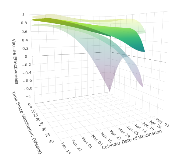
(a)

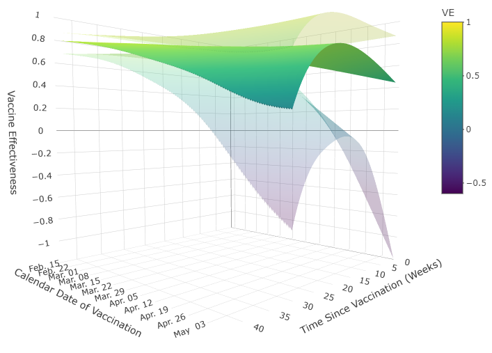
(b)

Figure 2: Estimated VE against severe COVID-19 or COVID-19-related death among Abruzzo residents aged 80 years or older between February 15, 2021 and December 18, 2021. The opaque surfaces depict the VE point estimates and the transparent surfaces the corresponding 95% Wald CIs. Panels (a) and (b) display the same surface from two vantage points.

Table 2: Estimated VE against severe COVID-19 or COVID-19-related death among Abruzzo residents aged 80 years or older ($n=120,778$) between February 15, 2021 and December 18, 2021. Results are presented for selected emulated trials and weeks since first dose. The starting date of each trial was as follows: trial $j=0$, February 15, 2021; trial $j=3$, March 8, 2021; trial $j=6$, March 29, 2021; and trial $j=9$, April 19, 2021.

Weeks since	$\widehat{VE}_{0}(k)$	$\widehat{VE}_{3}(k)$	$\widehat{VE}_{6}(k)$	$\widehat{VE}_{9}(k)$
first dose ($k$)	% (95% CI)
1	86 (73, 93)	79 (68, 87)	69 (40, 84)	56 (-27, 85)
7	87 (76, 93)	81 (72, 88)	73 (50, 86)	64 (7, 86)
14	87 (76, 93)	82 (72, 88)	76 (56, 86)	70 (26, 87)
21	86 (75, 93)	81 (71, 88)	76 (58, 86)	70 (32, 87)
28	85 (74, 92)	80 (70, 86)	72 (55, 82)	60 (23, 80)
34	84 (73, 91)	77 (67, 84)	63 (45, 75)	32 (-10, 58)

5 Discussion

Nested trial emulation has become increasingly popular in practice for drawing inference about treatment effects from observational data. Motivated by the need to assess the effects of COVID-19 vaccination outside of randomized trials, this paper develops NTE-based methods which allow treatment (vaccine) effects to vary on two different time scales, namely time since treatment initiation and calendar time. While motivated by vaccine studies, the methods could be applied in any setting where treatment effects may plausibly vary across both time scales.

The application evaluated effectiveness of a full course of COVID-19 vaccine versus remaining unvaccinated among elder residents of the Abruzzo region of Italy. It is difficult to directly compare these results with those of Acuti Martellucci et al. (2022) because the designs differ in several key aspects. Acuti Martellucci et al. estimated the effectiveness of a full course of COVID-19 vaccine versus remaining unvaccinated among individuals 60 years of age or older during the period January 31, 2021 through February 8, 2022. They estimated VE against COVID-19-related death to be 94% (95% CI:93% to 95%) and against severe COVID-19 to be 86% (95% CI:84% to 88%). For comparison, in the present analysis the estimated VE against the composite outcome at week 44 of trial 0 (i.e., February 15, 2021 through December 18, 2021) was 80% (95% CI:67% to 87%). However, direct comparison of these estimates is not straightforward because of differences in study period, target population, and outcome. The analyses also targeted different estimands. Acuti Martellucci et al. defined VE as one minus the adjusted odds ratio, while in this manuscript VE equals one minus the marginal risk ratio. Although the odds ratio approximates the risk ratio when the outcome is rare (Cornfield, 1951), the adjusted odds ratio does not in general equal the marginal odds ratio due to noncollapsibility (Daniel, Zhang, and Farewell, 2021).

The analysis presented in Section 4 draws new insights from the Abruzzo study database. Particularly, the analysis characterizes VE trends across calendar time and time since vaccination. These results suggest that for the vaccine regimen considered (i) VE peaked approximately 15-20 weeks after the first dose, and (ii) VE waned over the calendar time of the study. The combination of (i) and (ii) can result in meaningful differences in the protective effect of the vaccine, e.g., VE 14 weeks after the first dose in the earliest emulated trial was estimated to be 87%, whereas VE 34 weeks after the first dose in the later trials was estimated to be less than 40%. Understanding changes in VE from time of first dose is important for informing when booster doses should be recommended. Characterizing changes in VE over calendar time can guide decisions by policy makers and vaccine manufactures regarding the need for updated vaccine formulations.

There are several possible avenues for future work to build on the methods described here. Future methodological research could focus on NTE under relaxed assumptions. For example, machine learning approaches could be incorporated to relax the need for correctly specified parametric models (Westreich, Lessler, and Funk, 2010). In many infectious disease settings, an individual’s outcome may be affected by other individuals’ vaccination status, i.e., there may be interference (Hudgens and Halloran, 2008). In the presence of interference, unvaccinated individuals may benefit from indirect protection due to the level of vaccine coverage in the population. In turn, analyses that fail to account for interference may yield biased VE estimates. Future research could develop NTE methods that accommodate interference.

Additional future work could tailor the methods in Section 2 to a variety of COVID-19 VE applications. First, the methods could be easily adapted to evaluate other vaccine regimens such as booster doses. Second, observational databases may lack sufficient information to ensure conditional exchangeability because certain confounders are hard to measure, like social distancing practices and individual attitudes about vaccines (Schnitzer, 2022). Future work may develop sensitivity analyses for unmeasured confounding (Robins, Rotnitzky, and Scharfstein, 2000) customized for the NTE framework. Third, the present application relied on the treatment variation irrelevance assumption (Cole and Frangakis, 2009; VanderWeele, 2009), which states that potential outcomes remain unchanged under different versions of treatment. Specifically, the active vaccine regimen was defined such that individuals could choose a vaccine brand from among those available and receive a second dose any time within a specified time window. In turn, results reflect VE in a counterfactual setting where the distribution of vaccine brands is equal to the observed distribution among elder Abruzzo residents in 2021. Future research could explore VE under different counterfactual distributions (VanderWeele and Hernán, 2013), e.g., to compare VE across vaccine types.

Supplemental Materials

R and Python code developed for the simulation studies in Section 3 and the application in Section 4 is available at https://github.com/justindemonte/VE_NTE.

Appendix A Methodological Details

A.1 Identifiability

The target estimand $VE_{j}(k)$ is identifiable from the observable random variables under the assumptions stated in the main text. To see this, first note that $VE_{j}(k)$ is a function of the mean potential outcomes $E\{Y^{1}_{j}(k)\mid R_{j}(0)=1\}$ and $E\{Y^{0}_{j}(k)\mid R_{j}(0)=1\}$ (where the event $R_{j}(0)=1$ is conditioned on because potential outcomes $Y^{z}_{j}(k)$ are only defined when $R_{j}(0)=1$ for $z\in\{0,1\}$). Therefore, it suffices to show that $E\{Y_{j}^{z}(k)\mid R_{j}(0)=1\}$ is identifiable for $z\in\{0,1\}$. The identification derivation is a special case of Robins’s g-formula (Robins, 1986). In particular, letting $F(\boldsymbol{x}\mid R_{j}(0)=1)$ denote the conditional distribution of $X$ given $R_{j}(0)=1$, observe that $1-E\{Y_{j}^{z}(k)\mid R_{j}(0)=1\}$

$$= P\{Y_{j}^{z}(k)=0\mid R_{j}(0)=1\}]$$ (A.1)

$$= \int_{\boldsymbol{x}}P\{Y_{j}^{z}(k)=0\mid\boldsymbol{X}=\boldsymbol{x},R_{j}(0)=1\}dF(\boldsymbol{x}\mid R_{j}(0)=1)$$ (A.2)

$$= \int_{\boldsymbol{x}}P\{Y_{j}^{z}(k)=0\mid\boldsymbol{X}=\boldsymbol{x},Z_{j}=z,R_{j}(0)=1\}dF(\boldsymbol{x}\mid R_{j}(0)=1)$$ (A.3)

$$= \int_{\boldsymbol{x}}P\{Y_{j}^{z}(k)=0\mid\boldsymbol{X}=\boldsymbol{x},Z_{j}=z,Y_{j}(0)=0,R_{j}(0)=1\}dF(\boldsymbol{x}\mid R_{j}(0)=1)$$ (A.4)

$$= \int_{\boldsymbol{x}}P\{Y_{j}^{z}(k)=0\mid\boldsymbol{X}=\boldsymbol{x},Z_{j}=z,Y_{j}(0)=0,R_{j}(1)=1\}dF(\boldsymbol{x}\mid R_{j}(0)=1)$$ (A.5)

$$= \sum_{y=0}^{1}\int_{\boldsymbol{x}}P\{Y_{j}^{z}(k)=0\mid\boldsymbol{X}=\boldsymbol{x},Z_{j}=z,Y_{j}(1)=y,Y_{j}(0)=0,R_{j}(1)=1\}\times$$ (A.6)

$$dF(\boldsymbol{x}\mid R_{j}(0)=1)P\{Y_{j}(1)=y\mid\boldsymbol{X}=\boldsymbol{x},Z_{j}=z,Y_{j}(0)=0,R_{j}(1)=1\}$$

$$= \sum_{y=0}^{1}\int_{\boldsymbol{x}}P\{Y_{j}^{z}(k)=0\mid\boldsymbol{X}=\boldsymbol{x},Z_{j}=z,Y_{j}^{z}(1)=y,Y_{j}(0)=0,R_{j}(1)=1\}\times$$ (A.7)

$$dF(\boldsymbol{x}\mid R_{j}(0)=1)P\{Y_{j}(1)=y\mid\boldsymbol{X}=\boldsymbol{x},Z_{j}=z,Y_{j}(0)=0,R_{j}(1)=1\}$$

$$= \int_{\boldsymbol{x}}P\{Y_{j}^{z}(k)=0\mid\boldsymbol{X}=\boldsymbol{x},Z_{j}=z,Y_{j}(1)=0,R_{j}(1)=1\}\times$$ (A.8)

$$dF(\boldsymbol{x}\mid R_{j}(0)=1)P\{Y_{j}(1)=0\mid\boldsymbol{X}=\boldsymbol{x},Z_{j}=z,Y_{j}(0)=0,R_{j}(1)=1\}$$

$$= \int_{\boldsymbol{x}}P\{Y_{j}^{z}(k)=0\mid\boldsymbol{X}=\boldsymbol{x},Z_{j}=z,Y_{j}(1)=0,R_{j}(2)=1\}$$ (A.9)

$$dF(\boldsymbol{x}\mid R_{j}(0)=1)P\{Y_{j}(1)=0\mid\boldsymbol{X}=\boldsymbol{x},Z_{j}=z,Y_{j}(0)=0,R_{j}(1)=1\}$$

$$= \int_{\boldsymbol{x}}P\{Y_{j}^{z}(k)=0\mid\boldsymbol{X}=\boldsymbol{x},Z_{j}=z,Y_{j}(2)=0,R_{j}(2)=1\}\times$$ (A.10)

$$dF(\boldsymbol{x}\mid R_{j}(0)=1)\prod_{m=1}^{2}P\{Y_{j}(m)=0\mid\boldsymbol{X}=\boldsymbol{x},Z_{j}=z,Y_{j}(m-1)=0,R_{j}(m)=1\}$$

$$= \dots$$ (A.11)

$$= \int_{\boldsymbol{x}}P\{Y_{j}^{z}(k)=0\mid\boldsymbol{X}=\boldsymbol{x},Z_{j}=z,Y_{j}(k-1)=0,R_{j}(k)=1\}\times$$ (A.12)

$$dF(\boldsymbol{x}\mid R_{j}(0)=1)\prod_{m=1}^{k-1}P\{Y_{j}(m)=0\mid\boldsymbol{X}=\boldsymbol{x},Z_{j}=z,Y_{j}(m-1)=0,R_{j}(m)=1\}$$

$$= \int_{\boldsymbol{x}}P\{Y_{j}(k)=0\mid\boldsymbol{X}=\boldsymbol{x},Z_{j}=z,Y_{j}(k-1)=0,R_{j}(k)=1\}\times$$ (A.13)

$$dF(\boldsymbol{x}\mid R_{j}(0)=1)\prod_{m=1}^{k-1}P\{Y_{j}(m)=0\mid\boldsymbol{X}=\boldsymbol{x},Z_{j}=z,Y_{j}(m-1)=0,R_{j}(m)=1\},$$

where (A.2) follows from the law of total probability; (A.3) from conditional exchangeability; (A.4) because $R_{j}(0)=1$ (i.e., eligibility for trial $j$) implies $Y_{j}(0)=0$; and (A.5) by positivity and ignorable censoring. If $k=1$, $Y_{j}^{z}(k)$ in (A.5) can be replaced by $Y_{j}(k)$ by causal consistency, and the proof is done. Similarly, proof in the $k=2$ case follows from line (A.10) and causal consistency. The full proof is obtained by repeatedly applying reasoning in lines (A.5) through (A.8) and then invoking causal consistency to arrive at an expression that depends only on observed data. Line (A.6) follows by the law of total probability; (A.7) from causal consistency; and (A.8) because $P\{Y_{j}^{z}(k)=0\mid Y_{j}^{z}(0)=1,\cdot\}=0$ for any $k\geq 1$ and by causal consistency. Lines (A.9) through (A.11) illustrate how repeatedly applying the reasoning in lines (A.5) through (A.8), will yield the expression in (A.12). Line (A.13) follows from causal consistency. The final expression depends only on observed data.

A.2 Inverse probability weight estimation

Estimates of $e_{j}(\boldsymbol{X_{1}})$ can be obtained by fitting a pooled logistic regression model of the form

$$\text{logit}\{e_{j}(\boldsymbol{X_{1}};\boldsymbol{\zeta})\}=\boldsymbol{\zeta}\boldsymbol{g}(j,\boldsymbol{X_{1}})$$ (A.14)

via maximum likelihood, where $\boldsymbol{\zeta}$ is a vector of unknown regression parameters and $\boldsymbol{g}(j,\boldsymbol{X_{1}})$ is a column vector of functions of trial number and covariates. Similarly, estimates of $d_{jk}(Z_{j},\boldsymbol{X_{2}})$ can be obtained by fitting the pooled logistic regression model

$$\text{logit}\{d_{jk}(Z_{j},\boldsymbol{X_{2}};\boldsymbol{\kappa})\}=\boldsymbol{\kappa}\boldsymbol{h}(j,k,Z_{j},\boldsymbol{X_{2}})$$ (A.15)

via maximum likelihood where $\boldsymbol{\kappa}$ is a vector of unknown regression parameters and $\boldsymbol{h}(j,k,Z_{j},\boldsymbol{X_{2}})$ is a column vector containing functions of trial number, time on trial, vaccine regimen assignment in trial $j$, and covariates. The form of the right sides of (A.14) and (A.15) are specified by the analyst. If the effect of covariates on the propensity score and hazard of remaining uncensored are assumed to vary across trials, models can be specified to include trial-specific regression coefficients.

A.3 Asymptotic distribution of $\boldsymbol{\hat{\rho}}$

Letting $i$ index the set of $n$ individuals in the analytic cohort, $\boldsymbol{\hat{\theta}}$ is the solution to $\sum_{i=1}^{n}\boldsymbol{\psi}(\boldsymbol{O_{i}};\boldsymbol{\theta})=\boldsymbol{0}$ where

$$\boldsymbol{\psi}(\boldsymbol{O};\boldsymbol{\theta}) =\begin{pmatrix}\boldsymbol{\psi_{\zeta}}(\boldsymbol{O};\boldsymbol{\zeta})\\ \boldsymbol{\psi_{\kappa}}(\boldsymbol{O};\boldsymbol{\kappa})\\ \boldsymbol{\psi_{\alpha}}(\boldsymbol{O};\boldsymbol{\zeta},\boldsymbol{\kappa},\boldsymbol{\alpha})\\ \boldsymbol{\psi_{\rho}}(\boldsymbol{\alpha};\boldsymbol{\zeta},\boldsymbol{\kappa})\end{pmatrix},$$

$$\boldsymbol{\psi_{\zeta}}(\boldsymbol{O};\boldsymbol{\zeta}) =\sum_{j=S}^{S^{*}}R_{j}(0)\big{\{}Z_{j}-e_{j}(\boldsymbol{X_{1}};\boldsymbol{\zeta})\big{\}}\boldsymbol{g}(j,\boldsymbol{\boldsymbol{X_{1}}}),$$

$$\boldsymbol{\psi_{\kappa}}(\boldsymbol{O};\boldsymbol{\kappa}) =\sum_{j=S}^{S^{*}}\sum_{k=1}^{K_{j}}R_{j}(k-1)\{1-Y_{j}(k-1)\}\big{\{}R_{j}(k)-d_{jk}(Z_{j},\boldsymbol{X_{2}};\boldsymbol{\kappa})\big{\}}\boldsymbol{h}(j,k,Z_{j},\boldsymbol{X_{2}}),$$

$$\boldsymbol{\psi_{\alpha}}(\boldsymbol{O};\boldsymbol{\alpha}) =\sum_{j=S}^{S^{*}}\sum_{k=1}^{K_{j}}R_{j}(k)\{1-Y_{j}{(k-1)}\}W_{j}(k)\big{\{}Y_{j}(k)-\lambda_{j}^{Z_{j}}(k;\boldsymbol{\alpha})\big{\}}\boldsymbol{f}(j,k,Z_{j}),$$

$$\boldsymbol{\psi_{\boldsymbol{\rho}}}(\boldsymbol{\alpha};\boldsymbol{\zeta},\boldsymbol{\kappa}) =\begin{pmatrix}\boldsymbol{\rho}_{0}^{T}-\boldsymbol{\nu}_{0}(\boldsymbol{\alpha})\\ \boldsymbol{\rho}_{1}^{T}-\boldsymbol{\nu}_{1}(\boldsymbol{\alpha})\\ \vdots\\ \boldsymbol{\rho}_{J}^{T}-\boldsymbol{\nu}_{J}(\boldsymbol{\alpha})\\ \end{pmatrix},$$

$$\boldsymbol{\nu}_{j}(\boldsymbol{\alpha}) =\{{\nu}_{j}(1,\boldsymbol{\alpha}),{\nu}_{j}(2,\boldsymbol{\alpha}),...,{\nu}_{j}(K_{j},\boldsymbol{\alpha})\}^{T},$$

$$\nu_{j}(k,\boldsymbol{\alpha}) =\log\big{[}1-\prod_{m=1}^{k}\{1-\lambda_{j}^{1}(m)\}\big{]}-\log\big{[}1-\prod_{m=1}^{k}\{1-\lambda_{j}^{0}(m)\}\big{]},\text{ and}$$

$$\lambda_{j}^{z}(k) =\text{logit}^{-1}\{\boldsymbol{\alpha}\boldsymbol{f}(j,k,z)\}.$$

To see that the vector estimating equation $\boldsymbol{\psi}(\boldsymbol{O};\boldsymbol{\theta})$ is unbiased, consider the following. Let $e_{j}=e_{j}(\boldsymbol{X_{1}};\boldsymbol{\zeta})$, $d_{jk}=d_{jk}(Z_{j},\boldsymbol{X_{2}};\boldsymbol{\kappa})$, and $\boldsymbol{f}=\boldsymbol{f}(j,k,Z_{j})$. The score functions for correctly specified generalized linear models are unbiased (McCullagh and Nelder, 1989), i.e., $E\{\boldsymbol{\psi_{\zeta}}(\boldsymbol{O}$;$\boldsymbol{\zeta})\}$=$\boldsymbol{0}$ and $E\{\boldsymbol{\psi_{\kappa}}(\boldsymbol{O}$;$\boldsymbol{\kappa})\}$=$\boldsymbol{0}$. When models (A.14), (A.15), and the MSM for the hazard of the outcome are all correctly specified, $E\{\boldsymbol{\psi_{\alpha}}(\boldsymbol{O};\boldsymbol{\zeta},\boldsymbol{\kappa},\boldsymbol{\alpha})\}$ equals

$$E \bigg{[}\sum_{j=S}^{S^{*}}\sum_{k=1}^{K_{j}}R_{j}(k)\{1-Y_{j}(k-1)\}W_{j}(k)\{Y_{j}(k)-\lambda^{Z_{j}}_{j}(k)\}\boldsymbol{f}\bigg{]}$$

$$= \sum_{r=0}^{1}\sum_{y=0}^{1}\sum_{j=S}^{S^{*}}\sum_{k=1}^{K_{j}}E\big{[}R_{j}(k)\{1-Y_{j}(k-1)\}W_{j}(k)\{Y_{j}(k)-\lambda^{Z_{j}}_{j}(k)\}\mid R_{j}(k)=r,Y_{j}(k-1)=y\big{]}$$

$$\times P\{R_{j}(k)=r,Y_{j}(k-1)=y\}\boldsymbol{f}$$ (A.16)

$$= \sum_{j=S}^{S^{*}}\sum_{k=1}^{K_{j}}E\big{[}R_{j}(k)\{1-Y_{j}(k-1)\}W_{j}(k)\{Y_{j}(k)-\lambda^{Z_{j}}_{j}(k)\}\mid R_{j}(k)=1,Y_{j}(k-1)=0\big{]}$$

$$\times P\{R_{j}(k)=1,Y_{j}(k-1)=0\}\boldsymbol{f}$$ (A.17)

$$= \sum_{j=S}^{S^{*}}\sum_{k=1}^{K_{j}}a_{jk}E\bigg{[}\bigg{(}\dfrac{Z_{j}}{e_{j}}+\dfrac{1-Z_{j}}{1-e_{j}}\bigg{)}\{Y_{j}(k)-\lambda^{Z_{j}}_{j}(k)\}\mid R_{j}(k)=1,Y_{j}(k-1)=0\bigg{]}\boldsymbol{f}$$

$$= \sum_{j=S}^{S^{*}}\sum_{k=1}^{K_{j}}a_{jk}E\bigg{[}\bigg{\{}\dfrac{Z_{j}Y_{j}^{1}(k)}{e_{j}}+\dfrac{(1-Z_{j})Y_{j}^{0}(k)}{1-e_{j}}-\bigg{(}\dfrac{Z_{j}}{e_{j}}+\dfrac{1-Z_{j}}{1-e_{j}}\bigg{)}\lambda^{Z_{j}}_{j}(k)\bigg{\}}$$ (A.18)

$$\mid\{Z_{j}Y_{j}^{1}(k-1)+(1-Z_{j})Y_{j}^{0}(k-1)\}=0,R_{j}(k)=1\bigg{\}}\bigg{]}\boldsymbol{f}$$

$$= \sum_{j=S}^{S^{*}}\sum_{k=1}^{K_{j}}a_{jk}E_{\boldsymbol{X_{1}}}\bigg{(}E\big{\{}Y_{j}^{1}(k)\mid Y^{1}_{j}(k-1)=0,R_{j}(k)=1,\boldsymbol{X_{1}}\big{\}}\bigg{\{}\dfrac{E(Z_{j}\mid R_{j}(0)=1,\boldsymbol{X_{1}})}{e_{j}}\bigg{\}}$$

$$+E\{Y_{j}^{0}(k)\mid Y^{0}_{j}(k-1)=0,R_{j}(k)=1,\boldsymbol{X_{1}}\}\bigg{\{}\dfrac{1-E(Z_{j}\mid R_{j}(0)=1,\boldsymbol{X_{1}})}{1-e_{j}}\bigg{\}}$$ (A.19)

$$-\bigg{[}\dfrac{E\{Z_{j}\mid R_{j}(0)=1,\boldsymbol{X_{1}}\}}{e_{j}}\lambda^{Z_{j}}_{j}(k)+\dfrac{1-E\{Z_{j}\mid R_{j}(0)=1,\boldsymbol{X_{1}}\}}{1-e_{j}}\lambda^{Z_{j}}_{j}(k)\bigg{]}\bigg{)}\boldsymbol{f}$$

$$= \sum_{j=S}^{S^{*}}\sum_{k=1}^{K_{j}}a_{jk}\bigg{(}E_{\boldsymbol{X_{1}},Z_{j}}\big{[}E\{Y_{j}^{1}(k)\mid Y^{1}_{j}(k-1)=0,R_{j}(k)=1,\boldsymbol{X_{1}},Z_{j}=z\}-\lambda^{1}_{j}(k)\big{]}$$ (A.20)

$$+\big{[}E\{Y_{j}^{0}(k)\mid Y^{0}_{j}(k-1)=0,R_{j}(k)=1,\boldsymbol{X_{1}},Z_{j}=z\}-\lambda^{0}_{j}(k)\big{]}\bigg{)}\boldsymbol{f}$$

$$= \sum_{j=S}^{S^{*}}\sum_{k=1}^{K_{j}}a_{jk}\bigg{(}\big{[}E\{Y_{j}^{1}(k)\mid Y^{1}_{j}(k-1)=0\}-\lambda^{1}_{j}(k)\big{]}$$ (A.21)

$$+\big{[}E\{Y_{j}^{0}(k)\mid Y^{0}_{j}(k-1)=0\}-\lambda^{0}_{j}(k)\big{]}\bigg{)}\boldsymbol{f}$$

$$= \boldsymbol{0}$$

where $a_{jk}$ is a constant that depends on $(j,k)$. Line (A.16) follows from linearity of expectation and the law of total probability; (A.17) follows because given $R_{j}(k)=0$ or $Y_{j}(k-1)=1$ the summand is zero. Noting that $R_{j}(k)=1$ implies $R_{j}(k-1)=1$, line (A.18) holds by causal consistency; (A.19) holds by iterated expectation and conditional exchangeability; (A.20) by iterated expectation; and (A.21) by ignorable censoring and by undoing iterated expectation. Unbiasedness of $\boldsymbol{\psi_{\rho}}$ follows from the definitions of $VE_{j}(k)$ and $\boldsymbol{\rho}$ in (2) and Section 2.5.2 of the main text, respectively, and the assumption that all models are correctly specified.

Since the estimating equation vector is unbiased, it follows that, under certain regularity conditions, $\sqrt{n}(\boldsymbol{\hat{\theta}}-\boldsymbol{{\theta}_{0})}\xrightarrow{d}N\{\boldsymbol{0},V(\boldsymbol{{\theta}_{0}})\}$ as $n\rightarrow\infty$, where $\boldsymbol{\theta_{0}}$ is the true parameter value, $V({\boldsymbol{\theta_{0}}})=\mathbb{A}({\boldsymbol{\theta_{0}}})^{-1}\mathbb{B}({\boldsymbol{\theta_{0}}})\{\mathbb{A}(\boldsymbol{\theta_{0}})^{-1}\}^{T}$, $\mathbb{A}({\boldsymbol{\theta_{0}}})=E\{-\dot{\boldsymbol{\psi}}(\boldsymbol{O};\boldsymbol{\theta_{0}})\}$, $\mathbb{B}({\boldsymbol{\theta_{0}}})=E[{\boldsymbol{\psi}}(\boldsymbol{O};{\boldsymbol{\theta_{0}}})\{{\boldsymbol{\psi}}(\boldsymbol{O};\boldsymbol{\theta_{0}})\}^{T}]$, and ${\dot{\boldsymbol{\psi}}(\boldsymbol{O};{\boldsymbol{\theta}})=\partial{{\boldsymbol{\psi}}}(\boldsymbol{O};{\boldsymbol{\theta}})}/\partial{\boldsymbol{\theta}}$ (Stefanski and Boos, 2002).

A.4 Asymptotic distribution of $\hat{\beta}$

Estimating equations for $\boldsymbol{\hat{\theta}^{\dagger}}=(\boldsymbol{\hat{\zeta}},\boldsymbol{\hat{\kappa}},\boldsymbol{\hat{\alpha}^{*}},\hat{\beta})$ are given by

$$\boldsymbol{\psi}(\boldsymbol{O};\boldsymbol{\theta^{\dagger}}) =\begin{pmatrix}\boldsymbol{\psi_{\zeta}}(\boldsymbol{O};\boldsymbol{\zeta})\\ \boldsymbol{\psi_{\kappa}}(\boldsymbol{O};\boldsymbol{\kappa})\\ \boldsymbol{\psi_{\alpha}}(\boldsymbol{O};\boldsymbol{\zeta},\boldsymbol{\kappa},\boldsymbol{\alpha})\\ \psi_{\beta}{({\boldsymbol{\alpha}};\boldsymbol{\zeta},\boldsymbol{\kappa})}\end{pmatrix},$$

where

$$\psi_{\beta}{\boldsymbol{(}{\boldsymbol{\alpha}};\boldsymbol{\zeta},\boldsymbol{\kappa})} =\beta-\dfrac{\sum_{j=0}^{J}(j-\bar{j})({AUC}_{j}-\overline{{AUC}_{j}})}{\sum_{j=0}^{J}(j-\bar{j})^{2}},$$

where the overbar denotes an average (taken across $j$); ${AUC}_{j}=\sum_{k=1}^{K_{J}}VE_{j}(k)$; $VE_{j}(k)$ is a function of $\{\lambda_{j}^{0}(k),\lambda_{j}^{1}(k)\}$ given by (2) in the main text; and $\{\lambda_{j}^{0}(k),\lambda_{j}^{1}(k)\}$ depend on $({\boldsymbol{\alpha}};\boldsymbol{\zeta},\boldsymbol{\kappa})$ through the specified MSM for the hazard of the outcome. The arguments in Section A.3 can also be applied here to show $E\{\boldsymbol{\psi_{\zeta}}(\boldsymbol{O};\boldsymbol{\zeta})\}$=$\boldsymbol{0}$, $E\{\boldsymbol{\psi_{\kappa}}(\boldsymbol{O};\boldsymbol{\kappa})\}$=$\boldsymbol{0}$, and $E\{\boldsymbol{\psi_{\alpha}}(\boldsymbol{O}$;$\boldsymbol{\zeta},\boldsymbol{\kappa},\boldsymbol{\alpha})\}$=$\boldsymbol{0}$ under $H_{0}$, provided that the corresponding models are correctly specified. To see that $E\{\psi_{\beta}(\boldsymbol{\alpha})\}=0$, note that under $H_{0}$, $\beta=0$ and $\overline{{AUC}_{j}}={AUC}_{j}$ for all $j\in\{0,1,...,J\}$. Since $\boldsymbol{\hat{\theta}^{\dagger}}$ is the solution to an unbiased estimating equation, under certain regularity conditions (Stefanski and Boos, 2002), $\sqrt{n}(\boldsymbol{\hat{\theta}^{\dagger}}-\boldsymbol{{\theta}^{\dagger}_{0})}\xrightarrow{d}N\{\boldsymbol{0},V(\boldsymbol{{\theta}_{0}^{\dagger}})\}$ as $n\rightarrow\infty$, where $\boldsymbol{\theta_{0}^{\dagger}}$ is the true parameter value under $H_{0}$. The empirical sandwich estimator $\widehat{V}_{n}(\boldsymbol{\hat{\theta}^{\dagger}})$ can be used to consistently estimate $V(\boldsymbol{{\theta}_{0}^{\dagger}})$.

Appendix B Additional Simulation Results

Additional simulations were conducted to evaluate performance of the methods whenever models were specified to include flexible functions of time variables. Simulations were carried out under the same data generating process and scenarios described in the main text. For analyzing the simulated data, the following variables were transformed using restricted cubic spline bases with four knots at the 5th, 35th, 65th, and 95th percentiles (Harrell, 2015): trial number in the propensity score model; calendar time in the model for the hazard of remaining uncensored; both calendar time and time on trial in the model for the hazard of the outcome.

Results are presented in Table A.1. Bias was low and CI coverage was near the nominal level in all scenarios. For each replication and each scenario, a generalized Wald test was conducted for the TEH assumption $H_{0}$. The null hypothesis $H_{0}$ was true by design in scenario 1. One-sided generalized Wald tests of $H_{0}$ were rejected at the $0.05$ significance level in $4.6\%$ of scenario 1 replications. The null hypothesis was false by design in scenarios 2 and 3 and was rejected in $100\%$ of the replications. Results suggest that, under these simulation conditions, methods performed well when model specification included flexible functions of time.

Appendix Tables

Table A.1: Additional simulation study results by scenario across $3,000$ replications, $\tau=20$ time points of follow-up, and $n=50,000$. All time functions in the analytical models were specified using restricted cubic splines.

		True				95% CI
		value		ESE	ASE	coverage
Scenario	Estimand	(%)	Bias	$\times 10^{2}$	$\times 10^{2}$	(%)
1	$VE_{0}(5)$	90.3	0.0	12.3	12.5	96
	$VE_{3}(5)$	90.3	-0.1	6.2	6.4	95
	$VE_{6}(5)$	90.3	-0.1	7.7	7.9	95
	$VE_{9}(5)$	90.3	-0.1	9.7	9.8	95
	$VE_{12}(5)$	90.3	-0.0	11.9	12.0	95
	$VE_{5}(1)$	91.4	0.1	13.2	13.1	95
	$VE_{5}(4)$	90.7	-0.1	8.1	8.2	95
	$VE_{5}(8)$	88.9	0.0	5.3	5.4	95
	$VE_{5}(12)$	85.8	0.2	3.9	3.9	94
	$VE_{5}(15)$	81.9	-0.1	3.5	3.5	94
2	$VE_{0}(5)$	90.2	0.1	12.3	12.5	95
	$VE_{3}(5)$	87.9	-0.1	6.2	6.3	96
	$VE_{6}(5)$	83.3	0.1	7.0	7.1	96
	$VE_{9}(5)$	74.3	0.2	8.5	8.6	95
	$VE_{12}(5)$	56.1	-0.1	10.4	10.5	95
	$VE_{5}(1)$	88.4	-0.2	11.7	11.8	95
	$VE_{5}(4)$	86.1	-0.0	7.4	7.6	96
	$VE_{5}(8)$	81.6	0.1	5.1	5.1	95
	$VE_{5}(12)$	74.1	0.1	4.0	3.9	95
	$VE_{5}(15)$	65.2	0.1	3.6	3.5	94
3	$VE_{0}(5)$	89.0	0.1	11.6	11.7	95
	$VE_{3}(5)$	86.3	-0.4	5.8	5.8	93
	$VE_{6}(5)$	81.1	-0.4	6.5	6.5	94
	$VE_{9}(5)$	70.9	-0.0	7.7	7.9	95
	$VE_{12}(5)$	50.2	-0.3	9.2	9.3	95
	$VE_{5}(1)$	88.1	0.0	11.3	11.4	96
	$VE_{5}(4)$	84.8	-0.4	6.9	7.0	94
	$VE_{5}(8)$	76.3	0.1	4.5	4.6	95
	$VE_{5}(12)$	56.4	0.7	3.3	3.3	92
	$VE_{5}(15)$	21.5	-0.1	2.9	2.9	95
Abbreviations: ASE, average estimated standard error; ESE,
empirical standard error; CI, confidence interval

Table A.1: Specification and emulation of a sequence of nested trials to assess effectiveness of a full course of COVID-19 vaccine between February 15, 2021 and Dec. 18, 2021.

	Target trial specification	Target trial emulation
	Target trial specification	Target trial emulation
Abbreviation: NHS, National Health Service
(Table continued on next page)    Inclusion criteria	Resident of or domiciled in Abruzzo region of Italy on Jan. 1, 2020	Same
	Aged 80 years or older at time of enrollment	Alive according to NHS data and over 80 years of age at time of enrollment
Exclusion criteria	Positive SARS-CoV-2 swab prior to enrollment	Positive SARS-CoV-2 swab documented in NHS data prior to enrollment
	Severe COVID-19 disease (as diagnosed by a specialist physician and requiring hospitalization) prior to enrollment	Severe COVID-19 disease (as diagnosed by a specialist physician and requiring hospitalization) documented in NHS data prior to enrollment
	Received any dose of any COVID-19 vaccine prior to enrollment	Any dose of any COVID-19 vaccine documented in NHS data prior to enrollment
Vaccine regimens	Active regimen “receive first COVID-19 vaccine dose within seven days of enrollment, receive second dose by end of the recommended time window (42 days from first dose for Pfizer-BioNTech and Moderna (Centers for Disease Control and Prevention, 2021); 84 days from first dose for AstraZeneca (World Health Organization, 2022); a single dose of Janssen is counted as two doses), and receive no further COVID-19 vaccine doses” versus comparator “remain unvaccinated through Dec. 18, 2021”.	Same
Treatment assignment	Each week during the enrollment period (Feb. 15, 2021 to May 9, 2021), a pragmatic randomized trial will be initiated. On the first day of each trial, eligible individuals will be enrolled and assigned at random (with equal probability) to active regimen or comparator. Those assigned to active regimen may choose the vaccine brand they receive (from among those available to them, for each dose). They will be instructed to receive a first dose of their chosen vaccine within seven days and then follow the corresponding dosing schedule (as described above).	On Feb. 15, 2021, all eligible individuals will be “enrolled" in a hypothetical trial. Those who receive a first COVID-19 vaccine dose during the first week of the trial will be classified as receiving active regimen; all others will be classified as receiving comparator. A series of identical hypothetical trials will be initiated on the first day of each subsequent week through May. 9, 2021. Individuals may appear in multiple trials, provided they meet eligibility criteria.
Outcome	Severe COVID-19 disease (as diagnosed by a specialist physician and requiring hospitalization) or COVID-19-related death	Severe COVID-19 disease (as diagnosed by a specialist physician and requiring hospitalization) or death with a SARS-CoV-2 positive swab documented in NHS data
Follow up	Eligibility will be assessed and treatment will be randomly assigned on the first day of each trial. Participants are followed until the first of the following: 1. Experience of an event 2. Discontinuation of assigned vaccine regimen 3. Death without a SARS-CoV-2 positive swab 4. December 18, 2021	Same, except: 1. Discontinuation is defined in terms of the regimen an individual was observed to initiate at the start of an emulated trial. 2. At-risk status will be evaluated at a series of weekly hypothetical “study visits".
Non- compliance	Participants who discontinue their assigned treatment strategy will be censored. Participants’ observations will be censored on the day of the first occurrence of any of the following: 1. Receipt of first dose of any COVID-19 vaccine (for participants assigned to comparator) 2. Failure to complete a second dose by the end of the recommended time window (for participants assigned to active regimen who elected to receive Pfizer, Moderna, or AstraZeneca vaccine for their first dose) 3. Receipt of a booster dose of COVID-19 vaccine (a third dose For those who received 2 doses of Pfizer, Moderna, AstraZeneca or a combination of these vaccines or a second dose for those who received Janssen vaccine)	Same, except censoring will be handled separately per person-trial, noncompliance is defined in terms of the regimen an individual was observed to initiate at the start of an emulated trial, and censoring status will be updated at weekly hypothetical study visits.
Causal contrast	Per-protocol effect	Observational analog of the per-protocol effect
Analysis plan	Analyses will be analogous to those described in the main text. Since exchangeability of treatment groups is expected due to randomization, there will be no adjustment for measured confounders. Inverse probability weighting will be used to adjust for selection bias arising due to differential censoring (nonadherence and loss to follow up; administrative censoring is assumed to be noninformative). Estimates and 95% CIs for the VE surface across calendar time and time since vaccination will be calculated and reported for each trial.	Analyses will be conducted according to methods described in the main text. Inverse probability weighting will be used to adjust for confounding and differential censoring due to nonadherence and loss to follow up. All time variables will be coarsened to weeks. Specific analytical decisions are detailed in Section 4 of the main text. Estimates and 95% CIs for VE across calendar time and time since vaccination will be calculated and reported for each trial. A test of the TEH assumption, as defined in the main text, will be conducted.

References

- Aalen, Cook, and Røysland (2015) Aalen, O.O., Cook, R.J., & Røysland, K. (2015) Does Cox analysis of a randomized survival study yield a causal treatment effect? Lifetime Data Analysis, 21(4), 579–593.
- Acuti Martellucci et al. (2022) Acuti Martellucci, C., Flacco M.E., Soldato, G., Di Martino, G., Carota, R., Caponetti, A., et al. (2022) Effectiveness of COVID-19 vaccines in the general population of an Italian region before and during the omicron wave. Vaccines, 10(5), 662.
- Baden et al. (2021) Baden, L.R., Brandon, E., Kotloff, K., Frey, S., Novak, R., Diemert, D., et al. (2021) Efficacy and Safety of the mRNA-1273 SARS-CoV-2 Vaccine. New England Journal of Medicine. 384(5), 403–416.
- Boos and Stefanski (2012) Boos, D.D., & Stefanski, L.A. (2012) Essential statistical inference: Theory and methods, Dordrecht: Springer, pp. 334–336.
- Centers for Disease Control and Prevention (2021) Centers for Disease Control and Prevention. (2021) Interim clinical considerations for use of COVID-19 vaccines currently authorized in the United States. Available from: https://web.archive.org/web/20210527235512/https://www.cdc.gov/vaccines/covid-19/clinical-considerations/covid-19-vaccines-us.html [Accessed 20th March 2024]
- Cole and Frangakis (2009) Cole, S.R., & Frangakis, C.E. (2009) The consistency statement in causal inference: a definition or an assumption? Epidemiology, 20(1), 3–5.
- Cole and Hernán (2008) Cole, S.R., Hernán, M.A. (2008) Constructing inverse probability weights for marginal structural models. American Journal of Epidemiology, 168(6), 656–664.
- Cornfield (1951) Cornfield, J. (1951) A method of estimating comparative rates from clinical data. Applications to cancer of the lung, breast, and cervix. Journal of the National Cancer Institute, 11(6), 1269–1275.
- Cox (1958) Cox, D.R. (1958). Planning of experiments. New York: Wiley.
- Danaei et al. (2013) Danaei, G., García Rodríguez, L.A., Cantero, O.F., Logan, R., & Hernán, M.A. (2013) Observational data for comparative effectiveness research: an emulation of randomised trials of statins and primary prevention of coronary heart disease. Statistical Methods in Medical Research, 22(1), 70–96.
- Danaei et al. (2018) Danaei, G., García Rodríguez, L.A., Cantero, O.F., Logan, R.W., & Hernán, M.A. (2018) Electronic medical records can be used to emulate target trials of sustained treatment strategies. Journal of clinical epidemiology, 96, 12–22.
- Daniel, Zhang, and Farewell (2021) Daniel, R., Zhang, J., & Farewell, D. (2021). Making apples from oranges: Comparing noncollapsible effect estimators and their standard errors after adjustment for different covariate sets. Biometrical Journal, 63(3), 528–557.
- Ebinger et al. (2022) Ebinger, J.E., Joung, S., Liu, Y., Wu, M., Weber, B., Clagget, B., et al. (2022) Demographic and clinical characteristics associated with variations in antibody response to BNT162b2 COVID-19 vaccination among healthcare workers at an academic medical centre: a longitudinal cohort analysis BMJ Open,; 12, e059994.
- Falsey et al. (2021) Falsey, A.R., Sobieszczyk, M.E., Hirsch, I., Sproule, S., Robb, M.L., Corey, L., et al. (2021) Phase 3 Safety and Efficacy of AZD1222 (ChAdOx1 nCoV-19) Covid-19 Vaccine. New England Journal of Medicine, 385(25), 2348–2360.
- Gazit et al. (2023) Gazit, S., Saciuk, Y., Perez, G., Peretz, A., Stuart, E.A.,& Patalon, T. (2023) Hybrid immunity against reinfection with SARS-CoV-2 following a previous SARS-CoV-2 infection and single dose of the BNT162b2 vaccine in children and adolescents: A target trial emulation. Lancet Microbe, 4(7), e495–e505.
- Halloran, Longini, and Struchiner (2010) Halloran, M.E., Longini, I.M., & Struchiner, C.J. (2010) Design and analysis of vaccine studies. New York, NY: Springer, pp. 21–27.
- Harrell (2015) Harrell, F.E. (2015) Regression modeling strategies: With applications to linear models, logistic regression, and survival analysis, 2nd edition. Switzerland: Springer, pp. 24–28.
- Hernán (2010) Hernán, M.A. (2010). The hazards of hazard ratios. Epidemiology, 21(1), 13–15.
- Hernán et al. (2008) Hernán, M.A., Alonso, A., Logan, R., Grodstein, F., Michels, K.B., Stampfer, M.J., et al. (2008) Observational studies analyzed like randomized experiments: An application to postmenopausal hormone therapy and coronary heart disease. Epidemiology, 19(6), 766–779.
- Hernán and Robins (2016) Hernán, M.A.,& Robins, J.M. (2016) Using big data to emulate a target trial when a randomized trial is not available. American Journal of Epidemiology, 183(8), 758–64.
- Hernán and Robins (2020) Hernán, M.A. & Robins, J.M. (2020) Causal inference: What if, Boca Raton, Florida: Chapman and Hall, pp. 224-226.
- Hernán, Robins, and Garcia Rodríguez (2005) Hernán, M.A., Robins, J.M., & Garcia Rodríguez, L.A. (2016) Discussion on ‘Statistical issues arising in the Women’s Health Initiative’ by Prentice Ross L et al. Biometrics, 61(4), 922–930.
- Hernán et al. (2016) Hernán, M.A., Sauer, B.C., Hernández-Díaz, S., Platt, R., & Shrier, I. (2016) Specifying a target trial prevents immortal time bias and other self-inflicted injuries in observational analyses. Journal of Clinical Epidemiology, 79, 70–75.
- Hudgens and Halloran (2008) Hudgens, M.G., & Halloran, M.E. (2016) Toward causal inference with interference. Journal of the American Statistical Association, 103(482):832–842.
- Keogh et al. (2023) Keogh, R.H., Gran, J.M., Seaman, S.R., Davies, G., & Vansteelandt, S. (2023) Causal inference in survival analysis using longitudinal observational data: Sequential trials and marginal structural models. Statistics in Medicine, 42(13), 2191–2225.
- Lin et al. (2022) Lin, DY, Gu, Y., Wheeler, B., Young, H., Holloway, S., Sunny, S.K., Moore, Z., & Zeng, D. (2022) Effectiveness of COVID-19 vaccines over a 9-month period in North Carolina. New England Journal of Medicine, 386(10), 933–941.
- Martinussen, Vansteelandt, and Andersen (2020) Martinussen, T., Vansteelandt, S., & Andersen, P.K. (2020) Subtleties in the interpretation of hazard contrasts. Lifetime Data Analysis, 26(4), 833–855.
- McConeghy et al. (2022) McConeghy, K.W., Bardenheier, B., Huang, A.W., White, E.M., Feifer, R.A., Blackman, C., et al. (2022) Infections, hospitalizations, and deaths among US nursing home residents with vs without a SARS-CoV-2 vaccine booster. Journal of the American Medical Association Network Open, 5(12), e2245417.
- Petrone et al. (2023) Petrone, D., Mateo-Urdiales, A., Sacco, C., Riccardo, F., Bella, A., Ambrosio, L. et al. (2023) Reduction of the risk of severe COVID-19 due to Omicron compared to Delta variant in Italy (November 2021 - February 2022). International Journal of Infectious Diseases, 129, 135–141.
- Polack et al. (2021) Polack, F.P., Thomas, S.J., Kitchin, N., Absalon, J., Gurtman, A. Lockhart, S., et al. (2021) Safety and efficacy of the BNT162b2 mRNA COVID-19 vaccine. New England Journal of Medicine, 383(27), 2603–2615.
- Robertson, Steingrimsson, and Dahabreh (2022) Robertson, S.E., Steingrimsson, J.A., & Dahabreh, I.A. (2022) Using numerical methods to design simulations: Revisiting the balancing intercept. American Journal of Epidemiology. 191(7), 1283–1289.
- Robins and Finkelstein (2000) Robins, J.M., & Finkelstein, D.M. (2000) Correcting for noncompliance and dependent censoring in an AIDS Clinical Trial with inverse probability of censoring weighted (IPCW) log-rank tests. Biometrics, 56(3), 779–88.
- Robins, Hernán, and Brumback (2000) Robins, J.M., Hernán, M.A., & Brumback, B. (2000) Marginal structural models and causal inference in epidemiology. Epidemiology, 11(5), 550–60.
- Robins, Rotnitzky, and Scharfstein (2000) Robins, J. M., Rotnitzky, A., & Scharfstein, D. O. (2000). Sensitivity analysis for selection bias and unmeasured confounding in missing data and causal inference models. In Statistical models in epidemiology, the environment, and clinical trials. New York, NY: Springer New York, pp. 1-94
- Sadoff et al. (2021) Sadoff, J., Gray, G., Vandebosch, A., Cárdenas, V., Shukarev, G., Grinsztejn, B. et al. (2021) Safety and efficacy of single-Dose Ad26.COV2.S vaccine against COVID-19. The New England Journal of Medicine, 384(23), 2187–2201.
- Saul and Hudgens (2020) Saul, B.C. & Hudgens, M.G. (2020) The Calculus of M-Estimation in R with geex. Journal of Statistical Software, 92, 1–15.
- Schnitzer (2022) Schnitzer, M.E. (2022) Estimands and estimation of COVID-19 vaccine effectiveness under the test-negative design: Connections to causal inference. Epidemiology, 33(3), 325–333.
- Stefanski and Boos (2002) Stefanski, L.A. & Boos, D.D. (2002) The calculus of M-estimation. The American Statistician, 56(1), 29–38.
- Tahara et al. (2016) Tahara, M., Bürckert, J-P., Kanou, K., Maenaka, K., Muller, C.P., & Takeda, M. (2016) Measles virus hemagglutinin protein epitopes: The basis of antigenic stability. Viruses. 8(8), 216.
- VanderWeele (2009) VanderWeele, T.J. (2009) Concerning the consistency assumption in causal inference. Epidemiology, 20(6), 880–883.
- VanderWeele and Hernán (2013) VanderWeele T.J. & Hernán, M.A. Causal inference under multiple versions of treatment. Journal of Causal Inference, 1(1),1–20.
- Westreich, Lessler, and Funk (2010) Westreich, D., Lessler, J., & Funk. M,J. (2010) Propensity score estimation: neural networks, support vector machines, decision trees (CART), and meta-classifiers as alternatives to logistic regression. Journal of Clinical Epidemiology. 63(8), 826–833.
- World Health Organization (2022) World Health Organization (2022) The Oxford/AstraZeneca (ChAdOx1-S [recombinant] vaccine) COVID-19 vaccine: what you need to know. Available from: https://www.who.int/news-room/feature-stories/detail/the-oxford-astrazeneca-covid-19-vaccine-what-you-need-to-know [Accessed 20th March 2024]
- World Health Organization (2024) World Health Organization (2024) WHO Coronavirus (COVID-19) Dashboard. Available from: https://data.who.int/dashboards/covid19/cases?n=c [Accessed 20th March 2024]
- Zemella et al. (2024) Zemella, A., Beer, K., Ramm, F., Wenzel, D., Düx, A., Merkel, K., et al. (2024). Vaccine-induced neutralizing antibodies bind to the H protein of a historical measles virus. International Journal of Medical Microbiology. 314, 151607.
- Zivich et al. (2022) Zivich, P.N., Klose, M., Cole, S.R., Edwards, J.K., & Shook-Sa, B.E. (2022) Delicatessen: M-estimation in Python. ArXiv e-prints.
Acknowledgments
The authors would like to thank Samuel Rosin and Paul Zivich for helpful suggestions and Cecilia Acuti Martellucci, Maria Elena Flacco, Graziella Soldato, Giuseppe Di Martino, Roberto Carota, Antonio Caponetti, and Lamberto Manzoli for sharing the Abruzzo, Italy database. This research was supported by the NIH (R37 AI054165). The content is solely the responsibility of the authors and does not represent the official views of the NIH.