spacing=nonfrench

Chiral Corrections to the Gell-Mann-Oakes-Renner Relation from
QCD Sum Rules

ABSTRACT

We calculate the next-to-leading order corrections to the $SU(2)\otimes SU(2)$ and $SU(3)\otimes SU(3)$ Gell-Mann-Oakes-Renner relations. We use a pseudoscalar correlator calculated from Perturbative QCD up to five loops and use the QCD Finite Energy Sum Rules with integration kernels tuned to suppress the importance of the hadronic resonances. This leads to a substantial reduction in the systematic uncertainties from the experimentally unknown resonance spectral function. We use the method of Fixed Order and Fixed Renormalization Scale Perturbation Theory to compute the integrals. We calculate these corrections to be $\delta_{\pi}=0.060\pm 0.014$ and $\delta_{K}=0.64\pm 0.24$. As a result of these new values we predict the value of the light quark condensate $\left\langle{0|\bar{q}q|0}\right\rangle=-\left({266\pm 5{\text{ MeV}}}\right)^{3}$ and the Chiral Perturbation Theory low energy constant $H_{2}^{r}=-\left({4.9\pm 1.8}\right)\times 10^{-3}$. Results from this work have been published as: J. Bordes, C.A. Dominguez, P. Moodley, J. Pe$\widetilde{\text{n}}$arrocha and K. Schilcher, J. High Ener. Phys. 05 (2010) 064.

Contents

1. 1 Introduction
2. 2 A Low Energy Theorem
   1. 2.1 Hadronic Part
   2. 2.2 QCD Part
   3. 2.3 The Gell-Mann-Oakes-Renner Relation
3. 3 The QCD Finite Energy Sum Rule
4. 4 Integration in the Complex Plane
   1. 4.1 Fixed Order Perturbation Theory
   2. 4.2 Fixed Renormalization Scale Perturbation Theory
5. 5 The Resonance Contribution $\left.{\delta_{5}\left(R\right)}\right|_{RES}$
6. 6 Results
   1. 6.1 Frozen Order Results
      1. 6.1.1 $SU(2)\otimes SU(2)$
   2. 6.2 FOPT Results
      1. 6.2.1 $SU(2)\otimes SU(2)$
      2. 6.2.2 $SU(3)\otimes SU(3)$
   3. 6.3 Discussion of Results
7. 7 Conclusion
8. A Miscellaneous Material for the Gell-Mann-Oakes-Renner Relation
   1. A.1 A Step Towards Covariance
   2. A.2 Time Ordered Products
   3. A.3 Preparatory Work I
   4. A.4 Preparatory Work II
   5. A.5 Operator Identity
9. B Perturbative QCD Calculations
   1. B.1 $\Pi_{0}(z)$ Calculations
      1. B.1.1 One Loop Calculation
      2. B.1.2 Two Loop Calculation
      3. B.1.3 Three Loop Calculation
      4. B.1.4 Four Loop Calculation
      5. B.1.5 Five Loop Calculation
   2. B.2 $\Pi_{2}(z)$ Calculations
   3. B.3 C_u Calculation
   4. B.4 C_j Calculations
10. C Renormalization Group Equations for the coupling and mass
11. D A comment about the CIPT
12. E Coefficient fixing of $\Delta(z)$
13. F Perturbative QCD Integrals
14. G The Resonance Integrals
15. H Exact solution of the RGE for $\alpha_{s}$ up to fifth order

List of Figures

1. 1 Integration contour used for correlator. X indicates a pole and the broken line indicates a branch cut in the complex plane along the positive real axis corresponding to the resonances
2. 2 Results for $\psi_{5}(0)$(GeV⁴) [30] as a function of the energy $s$ in FSPT with $\mu^{2}=4$GeV². a, b and c correspond to polynomial orders 4, 5 and 6 respectively.
3. 3 Results for $\psi_{5}(0)$(GeV⁴) as a function of the energy $s$ in FOPT. We have neglected the two resonances. Starting from the top we have $\psi_{5}(s,0.365)$ and $\psi_{5}(s,0.397)$ respectively
4. 4 Results for $\delta_{\pi}$ as a function of the energy $s$ in FOPT. We have neglected the two resonances. Starting from the top we have $\delta_{\pi}(s,0.397)$ and $\delta_{\pi}(s,0.365)$ respectively
5. 5 Results for $\psi_{5}(0)$(GeV⁴) as a function of the energy $s$ in FOPT. We have included the two resonances with the weighting factor $\kappa=0.5$. Starting from the top we have $\psi_{5}(s,0.365)$ and $\psi_{5}(s,0.397)$ respectively
6. 6 Results for $\delta_{\pi}$ as a function of the energy $s$ in FOPT. We have included the two resonances with the weighting factor $\kappa=0.5$. Starting from the top we have $\delta_{\pi}(s,0.397)$ and $\delta_{\pi}(s,0.365)$ respectively
7. 7 Plot of the various contributors to $\delta_{\pi}$ for $\Lambda_{QCD}=0.365$ GeV. Starting from the top we have $\ln(\delta_{\pi}^{\pi 0})$, $\ln(\delta_{\pi}^{C_{j}})$, $\ln(\delta_{\pi}^{C_{u}})$ and $\ln(\delta_{\pi}^{\pi 2})$ respectively
8. 8 Plot of the various contributors to $\delta_{\pi}$ for $\Lambda_{QCD}=0.397$ GeV. Starting from the top we have $\ln(\delta_{\pi}^{\pi 0})$, $\ln(\delta_{\pi}^{C_{j}})$, $\ln(\delta_{\pi}^{C_{u}})$ and $\ln(\delta_{\pi}^{\pi 2})$ respectively
9. 9 Results for $\psi_{5}(0)$(GeV⁴) as a function of the energy $s$ in FOPT. We have neglected the two resonances. Starting from the top we have $\psi_{5}(s,0.365)$ and $\psi_{5}(s,0.397)$ respectively
10. 10 Results for $\delta_{\pi}$ as a function of the energy $s$ in FOPT. We have neglected the two resonances. Starting from the top we have $\delta_{K}(s,0.397)$ and $\delta_{K}(s,0.365)$ respectively
11. 11 Results for $\psi_{5}(0)$(GeV⁴) as a function of the energy $s$ in FOPT. We have included the two resonances with the weighting factor $\kappa=0.5$. Starting from the top we have $\psi_{5}(s,0.365)$ and $\psi_{5}(s,0.397)$ respectively
12. 12 Results for $\delta_{\pi}$ as a function of the energy $s$ in FOPT. We have included the two resonances with the weighting factor $\kappa=0.5$. Starting from the top we have $\delta_{K}(s,0.397)$ and $\delta_{K}(s,0.365)$ respectively
13. 13 Plot of the various contributors to $\delta_{K}$ for $\Lambda_{QCD}=0.365$ GeV. Starting from the top we have $\ln(\delta_{K}^{\pi 0})$, $\ln(\delta_{K}^{\pi 2})$, $\ln(\delta_{K}^{C_{j}})$ and $\ln(\delta_{K}^{C_{u}})$ respectively
14. 14 Plot of the various contributors to $\delta_{K}$ for $\Lambda_{QCD}=0.397$ GeV. Starting from the top we have $\ln(\delta_{K}^{\pi 0})$, $\ln(\delta_{K}^{\pi 2})$, $\ln(\delta_{K}^{C_{j}})$ and $\ln(\delta_{K}^{C_{u}})$ respectively
15. 15 Numerical solution to the RGE for $\alpha_{s}(0,0.397)=0.11266$, with the top curve the real part and the bottom the imaginary part of $\alpha_{s}$

List of Tables

1. 1 Tabulated values extracted from the plots 3 - 5 which are used to estimate $\delta_{\pi}$.
2. 2 Tabulated values extracted from the plots 9 - 12 which are used to estimate $\delta_{K}$.

1 Introduction

In recent years it has become generally accepted that the correct physical theory for the description of the strongly interacting particles is Quantum Chromodynamics (QCD). Initially there had been strong criticism against QCD since the fundamental constituents of the theory, the quarks and gluons, had never been observed in nature or in the laboratory. This is still the case today, but there have been many predictions from QCD about the bound states of these quarks (hadrons) which can be tested in the laboratory. Since there has been no analytic solution to QCD as yet, these predictions have been made possible by exploiting one of the key features of QCD, which is Asymptotic freedom and its closely related counterpart Confinement. These interesting features of QCD were discovered by Gross, Wilcek and Politzer [1, 2]. Confinement provides a theoretical explanation for why there are no hadronic colour multiplicity states observed in nature. The reason for this is, as the quarks move further away from each other, their interaction starts to increase i.e. the value of $\alpha_{s}$, the strong coupling (which sets the scale of the interaction), increases up to the point where there is so much energy in the two quark system that it is energetically more economical to bring two more quarks into existence from the vacuum and decrease the total energy of the system. For shorter distances between quarks the strong coupling goes to zero.

This allows us to use the tools from Perturbation theory to make an expansion of the equations of motion, which cannot be solved analytically (as yet), in terms of this small parameter $\alpha_{s}$. In this way we can extract information from QCD to get an approximate understanding of the behavior of the quarks and gluons.

The two main ways to compute hadronic parameters from QCD have been with the use of Lattice QCD were numerical solutions to the equations of motion are found. This is good since no approximations are made and solutions obtained are nearly exact, but since the computer is a black box we have no understanding about the subtle mechanisms at work in the theory. This is an undesirable feature of the results from Lattice QCD. The other way to extract information from the QCD equations of motion is the use of the QCD sum rules.

The idea of the QCD sum rules was developed in the late 1970’s by Shifman et al [3, 4] and has now become one of the work horses of analytic methods to extract information from QCD. QCD sum rules assume that confinement exists in QCD and tries to parameterize this effect. QCD sum rules are based on two ideas, the Operator Product Expansion (OPE) which separates the short and long distance quark-gluon interactions, and the application of Cauchy’s Theorem in the complex energy (squared) plane. The short distance interactions are calculated using Perturbative QCD and the long distance interaction, which are non-perturbative effects, are parameterized in terms of the vacuum condensates.

In this project we use the method of QCD sum rules to make a direct estimate of the breaking of the $SU(2)\otimes SU(2)$ and $SU(3)\otimes SU(3)$ Gell-Mann-Oakes-Renner relations. There have been previous attempts to calculate this symmetry breaking parameter [5, 6], but these have been indirect methods to estimate the breaking parameter $\delta_{\pi}$, with large uncertainties associated with them. The symmetry breaking parameter is also of great interest to the field of Chiral Perturbation Theory where $\delta_{\pi}$ is related to two of the theory’s low energy constants $L_{8}^{r}$ and $H_{2}^{r}$.

2 A Low Energy Theorem

The Gell-Mann, Oakes, Renner Relation (GMOR) is a low energy relation which comes from the global
$SU(N)\otimes SU(N)$ chiral symmetry which is present in the theory of strongly interacting particles. We give a proof for the relation below. For simplicity, we shall consider the case of the pion $\pi$ and hence $n=2$

2.1 Hadronic Part

We start with the hadronic pseudoscalar correlator which is the time-ordered product of the hadronic currents

$$\left.{\psi_{5}\left({q^{2}}\right)}\right|_{{\text{HAD}}}=i\int{e^{iq\cdot x}\left\langle{0\left|{T\left[{\partial^{\mu}A_{\mu}(x)\partial^{\nu}A_{\nu}^{\dagger}(0)}\right]}\right|0}\right\rangle dx}$$ (2.1.1)

since the Fock space has the property of completeness we can insert a state between the two currents without changing the correlator

$$\left.{\psi_{5}\left({q^{2}}\right)}\right|_{{\text{HAD}}}=i\sum\limits_{n}{\int{e^{iq\cdot x}\left\langle{0\left|{T\left[{\partial^{\mu}A_{\mu}(x)\left|n\right\rangle\left\langle n\right|\partial^{\nu}A_{\nu}^{\dagger}(0)}\right]}\right|0}\right\rangle}dx}$$ (2.1.2)

we will insert only the pion state and then truncate the series. From the Partial Conserved Axial Current(PCAC) [7, 8, 9] we have

$$\partial^{\mu}A_{\mu}\left(x\right)=\sqrt{2}f_{\pi}m_{\pi}^{2}\hat{\varphi}\left(x\right)$$ (2.1.3)

were $m_{\pi}$ and $f_{\pi}$ are the pion mass and the pion decay constant respectively. Inserting (2.1.3) into the correlator (2.1.1) we obtain

$$\left.{\psi_{5}\left({q^{2}}\right)}\right|_{{\text{HAD}}}=2f_{\pi}^{2}m_{\pi}^{4}i\int{e^{iq\cdot x}\left\langle{0\left|{T\left[{\hat{\varphi}\left(x\right)\hat{\varphi}^{\dagger}\left(0\right)}\right]}\right|0}\right\rangle d^{4}x}$$ (2.1.4)

The right-hand-side of (2.1.4) is just the Fourier transform of the vacuum-expectation-value(vev) of some operator. This operator is the Green’s function/propagator for the pion and can then be written as

$$i\Delta\left({x-y}\right)=\left\langle{0\left|{T\left[{\hat{\varphi}\left(x\right)\hat{\varphi}^{\dagger}\left(y\right)}\right]}\right|0}\right\rangle$$ (2.1.5)

were $x$ and $y$ are arbitrary spacetime points. We can then split the time ordered product (2.1.5) into two terms which depend on which event occurred first.

$$i\Delta\left({x-y}\right)=\Theta\left({x_{0}-y_{0}}\right)\left\langle{0\left|{\hat{\varphi}\left(x\right)\hat{\varphi}\left(y\right)}\right|0}\right\rangle+\Theta\left({y_{0}-x_{0}}\right)\left\langle{0\left|{\hat{\varphi}\left(y\right)\hat{\varphi}\left(x\right)}\right|0}\right\rangle\hfill$$ (2.1.6)

were $\Theta(x)$ is the Heaviside/Step function. The pion field can be written as a sum over the positive and negative energy states with appropriate creation and annihilation operators

$$\hat{\varphi}\left(x\right)=\sum\limits_{q}{\left[{\hat{a}_{q}\varphi_{\underset{\raise 2.10002pt\hbox{$\smash{\scriptscriptstyle-}$}}{q}}^{(+)}\left(x\right)+\hat{a}^{\dagger}_{q}\varphi_{-\underset{\raise 2.10002pt\hbox{$\smash{\scriptscriptstyle-}$}}{q}}^{(-)}\left(x\right)}\right]}$$ (2.1.7)

The $\varphi_{\underset{\raise 2.10002pt\hbox{$\smash{\scriptscriptstyle-}$}}{q}}^{(+)}\left(x\right),\varphi_{-\underset{\raise 2.10002pt\hbox{$\smash{\scriptscriptstyle-}$}}{q}}^{(-)}\left(x\right)$ are the positive and negative energy plane wave solutions. Inserting the $\pi$ fields(2.1.7) into the propagator(2.1.6).

$$i\Delta\left({x-y}\right)=\Theta\left({{x_{0}}-{y_{0}}}\right)\left\langle{0\left|{\sum\limits_{q}{\left[{{{\hat{a}}_{\underline{q}}}\varphi_{\underline{q}}^{(+)}\left(x\right)+\hat{a}_{\underline{q}}^{\dagger}\varphi_{-\underline{q}}^{(-)}\left(x\right)}\right]}\sum\limits_{q^{\prime}}{\left[{{{\hat{a}}_{\underline{q}^{\prime}}}\varphi_{\underline{q}^{\prime}}^{(+)}\left(y\right)+\hat{a}_{\underline{q}^{\prime}}^{\dagger}\varphi_{-\underline{q}^{\prime}}^{(-)}\left(y\right)}\right]}}\right|0}\right\rangle+$$

$$+\Theta\left({{y_{0}}-{x_{0}}}\right)\left\langle{0\left|{\sum\limits_{q^{\prime}}{\left[{{{\hat{a}}_{\underline{q}^{\prime}}}\varphi_{\underline{q}^{\prime}}^{(+)}\left(y\right)+\hat{a}_{\underline{q}^{\prime}}^{\dagger}\varphi_{-\underline{q}^{\prime}}^{(-)}\left(y\right)}\right]}\sum\limits_{q}{\left[{{{\hat{a}}_{\underline{q}}}\varphi_{\underline{q}}^{(+)}\left(x\right)+\hat{a}_{\underline{q}}^{\dagger}\varphi_{\underline{-q}}^{(-)}\left(x\right)}\right]}}\right|0}\right\rangle$$ (2.1.8)

since there is a product of sums and the sums are over different momenta we can collect the summations together and proceed with normal multiplication.

$$i\Delta\left({x-y}\right) = \Theta\left({{x_{0}}-{y_{0}}}\right)\left\langle{0\left|{\sum\limits_{q}{\sum\limits_{q^{\prime}}{\left[{\varphi_{\underline{q}}^{(+)}\left(x\right)\varphi_{\underline{q}^{\prime}}^{(+)}\left(y\right){{\hat{a}}_{\underline{q}}}{{\hat{a}}_{\underline{q}^{\prime}}}+\underline{\varphi_{\underline{q}}^{(+)}\left(x\right)\varphi_{-\underline{q}^{\prime}}^{(-)}\left(y\right){{\hat{a}}_{\underline{q}}}\hat{a}_{\underline{q}^{\prime}}^{\dagger}}}\right]}}}\right|0}\right\rangle+$$ (2.1.9)

$$\Theta\left({{x_{0}}-{y_{0}}}\right)\left\langle{0\left|{\sum\limits_{q}{\sum\limits_{q^{\prime}}{\left[{\varphi_{-\underline{q}}^{(-)}\left(x\right)\varphi_{\underline{q}^{\prime}}^{(+)}\left(y\right)\hat{a}_{\underline{q}}^{\dagger}{{\hat{a}}_{\underline{q}^{\prime}}}+\varphi_{-\underline{q}}^{(-)}\left(x\right)\varphi_{-\underline{q}^{\prime}}^{(-)}\left(y\right)\hat{a}_{\underline{q}}^{\dagger}\hat{a}_{\underline{q}^{\prime}}^{\dagger}}\right]}}}\right|0}\right\rangle+$$

$$\Theta\left({{y_{0}}-{x_{0}}}\right)\left\langle{0\left|{\sum\limits_{q}{\sum\limits_{q^{\prime}}{\left[{\varphi_{\underline{q}}^{(+)}\left(x\right)\varphi_{\underline{q}^{\prime}}^{(+)}\left(y\right){{\hat{a}}_{\underline{q}^{\prime}}}{{\hat{a}}_{\underline{q}}}+\underline{\varphi_{\underline{q}^{\prime}}^{(+)}\left(y\right)\varphi_{-\underline{q}}^{(-)}\left(x\right){{\hat{a}}_{\underline{q}^{\prime}}}\hat{a}_{\underline{q}}^{\dagger}}}\right]}}}\right|0}\right\rangle+$$

$$\Theta\left({{y_{0}}-{x_{0}}}\right)\left\langle{0\left|{\sum\limits_{q}{\sum\limits_{q^{\prime}}{\left[{\varphi_{-\underline{q}^{\prime}}^{(-)}\left(y\right)\varphi_{\underline{q}}^{(+)}\left(x\right)\hat{a}_{\underline{q}}^{\prime{\dagger}}{{\hat{a}}_{\underline{q}}}+\varphi_{-\underline{q}^{\prime}}^{(-)}\left(y\right)\varphi_{-\underline{q}}^{(-)}\left(x\right)\hat{a}_{\underline{q}^{\prime}}^{\dagger}\hat{a}_{\underline{q}}^{\dagger}}\right]}}}\right|0}\right\rangle$$

all terms in the above expansion are zero except the underlined ones. These are the only terms which contain the right combination of creation and annihilation operators which connect the vacuum to the vacuum. This can be seen if we use the commutation relation [10]

$$\left[{{{\hat{a}}_{\underline{q}}};\hat{a}_{\underline{q}^{\prime}}^{\dagger}}\right]={\delta_{qq^{\prime}}}$$

The propagator is then

$$i\Delta\left({x-y}\right)=\Theta\left({x_{0}-y_{0}}\right)\sum\limits_{q}{\left[{\varphi_{\underset{\raise 2.10002pt\hbox{$\smash{\scriptscriptstyle-}$}}{q}}^{(+)}\left(x\right)\varphi_{-\underline{q}}^{(-)}\left(y\right)}\right]}+\Theta\left({y_{0}-x_{0}}\right)\sum\limits_{q}{\left[{\varphi_{\underline{q}}^{(+)}\left(y\right)\varphi_{-\underline{q}}^{(-)}\left(x\right)}\right]}$$ (2.1.10)

One of the sums over the momenta has been ‘killed’ by the delta function which picked for us only one momentum state $q^{\prime}=q$. We now proceed by using the plane wave solutions

$$\varphi_{\pm\underline{q}}^{(\pm)}\left(x\right)=C_{\pm\underline{q}}e^{\mp iq^{\mu}\cdot x_{\mu}}$$ (2.1.11)

with the coefficient

$$C_{\pm\underline{q}}=\frac{1}{{\left({2\pi}\right)^{{\raise 1.50694pt\hbox{$\scriptstyle 3$}\kern-0.70004pt/\kern-1.04996pt\lower 0.75346pt\hbox{$\scriptstyle 2$}}}}}\frac{1}{{\sqrt{2E_{\pm\underline{q}}}}}$$ (2.1.12)

and the energy $E_{\pm\underline{q}}=\sqrt{\underline{q}^{2}+m^{2}}$, since the energy is invariant of the sign of the momentum, the coefficient is in turn also invariant and thus only the exponential carries the sign which distinguishes the positive and negative plane waves. We will go from a discrete set of $q$ to the continuum and the sum over the $q$ states will change to an integral over the continuous momenta $q$. We shall also henceforth drop the sign in the energy and the coefficient. Using (2.1.11) in the propagator (2.1.10) we obtain

$$i\Delta\left({x-y}\right) =\Theta\left({x_{0}-y_{0}}\right)\int{C_{\underline{q}}^{2}e^{-iq^{\mu}\cdot\left({x_{\mu}-y_{\mu}}\right)}d^{3}q}+\Theta\left({y_{0}-x_{0}}\right)\int{C_{\underline{q}}^{2}e^{-iq^{\mu}\cdot\left({y_{\mu}-x_{\mu}}\right)}d^{3}q}$$

$$=\int{\Theta\left({x_{0}-y_{0}}\right)C_{\underline{q}}^{2}e^{-iE_{\underline{q}}\cdot\left({x_{0}-y_{0}}\right)}e^{i\underline{q}\cdot\left({\underline{x}-\underline{y}}\right)}d^{3}q}+\int{\Theta\left({y_{0}-x_{0}}\right)C_{\underline{q}}^{2}e^{-iE_{\underline{q}}\cdot\left({y_{0}-x_{0}}\right)}e^{i\underline{q}\cdot\left({\underline{y}-\underline{x}}\right)}d^{3}q}$$

$$=\int{\Theta\left({x_{0}-y_{0}}\right)C_{\underline{q}}^{2}e^{-iE_{\underline{q}}\cdot\left({x_{0}-y_{0}}\right)}e^{-i\underline{q}\cdot\left({\underline{y}-\underline{x}}\right)}d^{3}q}+\underline{\int{\Theta\left({y_{0}-x_{0}}\right)C_{\underline{q}}^{2}e^{-iE_{\underline{q}}\cdot\left({y_{0}-x_{0}}\right)}e^{i\underline{q}\cdot\left({\underline{y}-\underline{x}}\right)}d^{3}q}}$$ (2.1.13)

making the change of variables $q\to-q$ for the second term which is underlined in (2.1.13) and noting the earlier comment of the invariance of the energy and coefficients under a change in sign in the momenta we arrive at

$$i\Delta\left({x-y}\right) = \int{\Theta\left({x_{0}-y_{0}}\right)C_{\underline{q}}^{2}e^{-iE_{\underline{q}}\cdot\left({x_{0}-y_{0}}\right)}e^{-i\underline{q}\cdot\left({\underline{y}-\underline{x}}\right)}d^{3}q}+^{*}\int{\Theta\left({y_{0}-x_{0}}\right)C_{\underline{q}}^{2}e^{-iE_{\underline{q}}\cdot\left({y_{0}-x_{0}}\right)}e^{-i\underline{q}\cdot\left({\underline{y}-\underline{x}}\right)}d^{3}q}$$ (2.1.14)

$$= \int{C_{\underline{q}}^{2}e^{-i\underline{q}\cdot\left({\underline{y}-\underline{x}}\right)}\left[{\Theta\left({x_{0}-y_{0}}\right)e^{-iE_{\underline{q}}\cdot\left({x_{0}-y_{0}}\right)}+\Theta\left({y_{0}-x_{0}}\right)e^{-iE_{\underline{q}}\cdot\left({y_{0}-x_{0}}\right)}}\right]d^{3}q}$$

* A subtle point to note about the change of variables here: even though there will be an overall negative sign coming from the differential $-d^{3}q$, we suppress the integrals signs denoting only one instead of a multitude, in this case there are three integrals that need to be done but with the change of variables we also swapped the three integration bounds which in turn gives $(-1)^{3}$ and with the negative sign from the differential leads to an overall positive sign.

$$X\equiv\Theta\left({x_{0}-y_{0}}\right)e^{-iE_{\underset{\raise 1.50002pt\hbox{$\smash{\scriptscriptstyle-}$}}{q}}\cdot\left({x_{0}-y_{0}}\right)}+\Theta\left({y_{0}-x_{0}}\right)e^{-iE_{\underset{\raise 1.50002pt\hbox{$\smash{\scriptscriptstyle-}$}}{q}}\cdot\left({y_{0}-x_{0}}\right)}$$ (2.1.15)

leading to

$$i\Delta\left({x-y}\right)=\int{C_{\underline{q}}^{2}e^{-i\underline{q}\cdot\left({\underline{y}-\underline{x}}\right)}Xd^{3}q}$$ (2.1.16)

We need (2.1.16) to be a Lorentz covariant object so we will need to go to the complex plane ($\mathbb{C}$) to accomplish this task. We can write $X$ as

$$X=\frac{{2E}}{{2\pi i}}\int\limits_{-\infty}^{\infty}{\frac{{e^{-i\left({x_{0}-y_{0}}\right)q_{0}}}}{{m_{\pi}^{2}-q^{2}-i\varepsilon^{\prime}}}dq_{0}}$$ (2.1.17)

See Appendix A.1 for details. Substituting (2.1.17) into (2.1.16) we obtain

$$i\Delta\left({x-y}\right) = \int{\frac{{2E}}{{2\pi i}}C_{\underline{q}}^{2}\frac{{e^{-i\left({x_{0}-y_{0}}\right)q_{0}}e^{i\underline{q}\cdot\left({\underline{x}-\underline{y}}\right)}}}{{m_{\pi}^{2}-q^{2}-i\varepsilon^{\prime}}}dq_{0}d^{3}q}$$ (2.1.18)

$$= \int{\frac{{2E}}{{2\pi i}}C_{\underline{q}}^{2}\frac{{e^{-i\left[{q_{0}\left({x_{0}-y_{0}}\right)-\underline{q}\cdot\left({\underline{x}-\underline{y}}\right)}\right]}}}{{m_{\pi}^{2}-q^{2}-i\varepsilon^{\prime}}}dq_{0}d^{3}q}$$

$$= \int{\frac{{2E}}{{2\pi i}}C_{\underline{q}}^{2}\frac{{e^{-iq_{\mu}\left({x^{\mu}-y^{\mu}}\right)}}}{{m_{\pi}^{2}-q^{2}-i\varepsilon^{\prime}}}d^{4}q}$$

$$= \int{\frac{{2E}}{{2\pi i}}C_{\underline{q}}^{2}\frac{{e^{-iq\cdot\left({x-y}\right)}}}{{m_{\pi}^{2}-q^{2}-i\varepsilon^{\prime}}}d^{4}q}$$

inserting the coefficient (2.1.12) into (2.1.18) leads to

$$i\Delta\left({x-y}\right) = \int{\frac{{2E}}{{2\pi i}}\frac{1}{{\left({2\pi}\right)^{3}}}\frac{1}{{2E}}\frac{{e^{-iq\cdot\left({x-y}\right)}}}{{m_{\pi}^{2}-q^{2}-i\varepsilon^{\prime}}}d^{4}q}$$ (2.1.19)

$$= \frac{1}{{\left({2\pi}\right)^{4}}}\int{e^{-iq\cdot\left({x-y}\right)}\frac{{-i}}{{m_{\pi}^{2}-q^{2}-i\varepsilon^{\prime}}}d^{4}q}$$

$$= \frac{1}{{\left({2\pi}\right)^{4}}}\int{e^{-iq\cdot\left({x-y}\right)}\frac{i}{{q^{2}-m_{\pi}^{2}+i\varepsilon^{\prime}}}d^{4}q}$$

(2.1.19) is now a Lorentz covariant object and retains its form in all inertial reference frames. We note now that the right-hand-side of (2.1.19) is just the Fourier transform of the propagator from momentum space to coordinate space. The propagator in momentum is then simply

$$\Delta\left(q\right)=\frac{1}{{q^{2}-m_{\pi}^{2}+i\varepsilon^{\prime}}}$$ (2.1.20)

Now looking back at the correlator (2.1.4) and the definition of the propagator (2.1.5) which is shown below

$$\left.{\psi_{5}\left({q^{2}}\right)}\right|_{{\text{HAD}}}=2f_{\pi}^{2}m_{\pi}^{4}i\int{e^{iq\cdot x}\left\langle{0\left|{T\left[{\hat{\varphi}\left(x\right)\hat{\varphi}^{\dagger}\left(0\right)}\right]}\right|0}\right\rangle d^{4}x}$$ (2.1.21)

$$i\Delta\left({x-y}\right)=\left\langle{0\left|{T\left[{\hat{\varphi}\left(x\right)\hat{\varphi}^{\dagger}\left(y\right)}\right]}\right|0}\right\rangle$$ (2.1.22)

substituting (2.1.22) into (2.1.21) we obtain

$$\left.{\psi_{5}\left({q^{2}}\right)}\right|_{{\text{HAD}}}=-2f_{\pi}^{2}m_{\pi}^{4}\int{e^{iq\cdot x}\Delta\left(x-y\right)d^{4}x}$$ (2.1.23)

we note now that the right-hand-side of (2.1.23) is just the Fourier transform of the propagator from coordinate space to momentum space but we know what this transform is in momentum space, it is (2.1.20) for the pion $\pi^{0}$, which leads to

$$\left.{\psi_{5}\left({q^{2}}\right)}\right|_{{\text{HAD}}}=-2f_{\pi}^{2}m_{\pi}^{4}\frac{1}{{q^{2}-m_{\pi}^{2}+i\varepsilon^{\prime}}}$$ (2.1.24)

and finally in the low energy limit and $\varepsilon^{\prime}\rightarrow 0$

$$\left.{\psi_{5}\left({0}\right)}\right|_{{\text{HAD}}}=2f_{\pi}^{2}m_{\pi}^{2}$$ (2.1.25)

2.2 QCD Part

We now turn to the QCD correlator. Starting from the axial two point correlating function of quark currents

$$\Pi_{\mu\nu}^{5}=i\int{e^{iq\cdot x}\left\langle{0\left|{T\left[{A_{\mu}\left(x\right)A_{\nu}^{\dagger}\left(0\right)}\right]}\right|0}\right\rangle d^{4}x}$$ (2.2.1)

the time ordered product can be expressed differently as

$$T\left[{A_{\mu}\left(x\right)A_{\nu}^{\dagger}\left(0\right)}\right]=\left[{A_{\mu}\left(x\right);A_{\nu}^{\dagger}\left(0\right)}\right]\Theta\left({x_{0}}\right)+A_{\nu}^{\dagger}\left(0\right)A_{\mu}\left(x\right)$$ (2.2.2)

(See Appendix A.2 for proof.) Inserting the time ordered product (2.2.2) into (2.2.1) we obtain

$$\Pi_{\mu\nu}^{5}=i\int{e^{iq\cdot x}\left\langle{0\left|\left[{A_{\mu}\left(x\right);A_{\nu}^{\dagger}\left(0\right)}\right]\Theta\left({x_{0}}\right)+A_{\nu}^{\dagger}\left(0\right)A_{\mu}\left(x\right)\right|0}\right\rangle d^{4}x}$$ (2.2.3)

we now apply the momentum operator

$$q^{\mu}=-i\frac{\partial}{{\partial x_{\mu}}}=i\partial^{\mu}$$ (2.2.4)

to (2.2.3)

$$q^{\mu}\Pi_{\mu\nu}^{5}=-i^{2}\partial^{\mu}\int{e^{iq\cdot x}\left\langle{0\left|\left[{A_{\mu}\left(x\right);A_{\nu}^{\dagger}\left(0\right)}\right]\Theta\left({x_{0}}\right)+A_{\nu}^{\dagger}\left(0\right)A_{\mu}\left(x\right)\right|0}\right\rangle d^{4}x}$$ (2.2.5)

since the fields are local the integral in (2.2.5) yields a function of $q$, acting on it with the momentum operator gives zero which leads to

$$0 = -{i^{2}}\int{{\partial^{\mu}}\left\{{{e^{iq\cdot x}}\left\langle{0\left|{\left[{{A_{\mu}}\left(x\right);A_{\nu}^{\dagger}\left(0\right)}\right]\Theta\left({{x_{0}}}\right)+A_{\nu}^{\dagger}\left(0\right){A_{\mu}}\left(x\right)}\right|0}\right\rangle}\right\}{d^{4}}x}$$ (2.2.6)

$$= {q^{\mu}}\underline{i\int{{e^{iq\cdot x}}\left\langle{0\left|{\left[{{A_{\mu}}\left(x\right);A_{\nu}^{\dagger}\left(0\right)}\right]\Theta\left({{x_{0}}}\right)+A_{\nu}^{\dagger}\left(0\right){A_{\mu}}\left(x\right)}\right|0}\right\rangle{d^{4}}x}}$$

$$+ \int{{e^{iq\cdot x}}\left\langle{0\left|{\underline{\left[{{\partial^{\mu}}{A_{\mu}}\left(x\right);A_{\nu}^{\dagger}\left(0\right)}\right]\Theta\left({{x_{0}}}\right)}+\left[{{A_{\mu}}\left(x\right);A_{\nu}^{\dagger}\left(0\right)}\right]{\partial^{\mu}}\Theta\left({{x_{0}}}\right)+\underline{A_{\nu}^{\dagger}\left(0\right){\partial^{\mu}}{A_{\mu}}\left(x\right)}}\right|0}\right\rangle{d^{4}}x}$$

we note that the first underlined term in (2.2.6 ) is $\Pi_{\mu\nu}^{5}$ in (2.2.3) and interestingly the second and third underlined terms together form a time-ordered product

$$\left[{{\partial^{\mu}}{A_{\mu}}\left(x\right);A_{\nu}^{\dagger}\left(0\right)}\right]\Theta\left({{x_{0}}}\right)+A_{\nu}^{\dagger}\left(0\right){\partial^{\mu}}{A_{\mu}}\left(x\right)=T\left[{{\partial^{\mu}}{A_{\mu}}\left(x\right)A_{\nu}^{\dagger}\left(0\right)}\right]$$ (2.2.7)

which leads to

$$0 ={q^{\mu}}\Pi_{{}_{\mu\nu}}^{5}+\int{{e^{iq\cdot x}}\left\langle{0\left|{T\left[{{\partial^{\mu}}{A_{\mu}}\left(x\right)A_{\nu}^{\dagger}\left(0\right)}\right]}\right|0}\right\rangle{d^{4}}x}+\int{{e^{iq\cdot x}}\left\langle{0\left|{\left[{{A_{\mu}}\left(x\right);A_{\nu}^{\dagger}\left(0\right)}\right]{\partial^{\mu}}\Theta\left({{x_{0}}}\right)}\right|0}\right\rangle{d^{4}}x}$$

$$={q^{\mu}}\Pi_{{}_{\mu\nu}}^{5}+\int{{e^{iq\cdot x}}\left\langle{0\left|{T\left[{{\partial^{\mu}}{A_{\mu}}\left(x\right)A_{\nu}^{\dagger}\left(0\right)}\right]}\right|0}\right\rangle{d^{4}}x}+\int{{e^{iq\cdot x}}\left\langle{0\left|{\left[{{A_{0}}\left(x\right);A_{\nu}^{\dagger}\left(0\right)}\right]{\partial^{0}}\Theta\left({{x_{0}}}\right)}\right|0}\right\rangle{d^{4}}x}$$ (2.2.8)

but the derivative of the Heaviside function leads to the delta function i.e. ${\partial^{0}}\Theta\left({{x_{0}}}\right)=\delta\left({{x_{0}}}\right)$ and defining the following functions:

$$\Pi_{{}_{\nu}}^{5} \equiv -\int{{e^{iq\cdot x}}\left\langle{0\left|{T\left[{{\partial^{\mu}}{A_{\mu}}\left(x\right)A_{\nu}^{\dagger}\left(0\right)}\right]}\right|0}\right\rangle{d^{4}}x}$$ (2.2.9)

$$\Delta_{{}_{\nu}}^{5} \equiv \int{{e^{iq\cdot x}}\left\langle{0\left|{\left[{{A_{0}}\left(x\right);A_{\nu}^{\dagger}\left(0\right)}\right]\delta\left({{x_{0}}}\right)}\right|0}\right\rangle{d^{4}}x}$$ (2.2.10)

and substituting into (2.2.8) gives us the Ward(I) identity

$$0={q^{\mu}}\Pi_{{}_{\mu\nu}}^{5}-\Pi_{{}_{\nu}}^{5}+\Delta_{{}_{\nu}}^{5}$$ (2.2.11)

We can express (2.2.9) as

$$\Pi_{{}_{\nu}}^{5}=\int{{e^{-iq\cdot x}}\left\langle{0\left|{T\left[{A_{\nu}^{\dagger}\left(x\right){\partial^{\mu}}{A_{\mu}}\left(0\right)}\right]}\right|0}\right\rangle{d^{4}}x}$$ (2.2.12)

See Appendix A.3 for details. We now apply the momentum operator (2.2.4) to (2.2.12). Since the fields are local the derivative yields zero

$$0 = -i\partial^{\nu}\int{e^{-iq\cdot x}\left\langle{0\left|{T\left[{A_{\nu}^{\dagger}\left(x\right)\partial^{\mu}A_{\mu}\left(0\right)}\right]}\right|0}\right\rangle d^{4}x}$$ (2.2.13)

$$= -i\int{\partial^{\nu}\left\{{e^{-iq\cdot x}\left\langle{0\left|{T\left[{A_{\nu}^{\dagger}\left(x\right)\partial^{\mu}A_{\mu}\left(0\right)}\right]}\right|0}\right\rangle}\right\}d^{4}x}$$

$$= -i\int{\left\{{-iq^{\nu}e^{-iq\cdot x}\left\langle{0\left|{T\left[{A_{\nu}^{\dagger}\left(x\right)\partial^{\mu}A_{\mu}\left(0\right)}\right]}\right|0}\right\rangle+e^{-iq\cdot x}\left\langle{0\left|{\partial^{\nu}T\left[{A_{\nu}^{\dagger}\left(x\right)\partial^{\mu}A_{\mu}\left(0\right)}\right]}\right|0}\right\rangle}\right\}d^{4}x}$$

$$= -q^{\nu}\underline{\int{e^{-iq\cdot x}\left\langle{0\left|{T\left[{A_{\nu}^{\dagger}\left(x\right)\partial^{\mu}A_{\mu}\left(0\right)}\right]}\right|0}\right\rangle d^{4}x}}-i\int{e^{-iq\cdot x}\left\langle{0\left|{\partial^{\nu}T\left[{A_{\nu}^{\dagger}\left(x\right)\partial^{\mu}A_{\mu}\left(0\right)}\right]}\right|0}\right\rangle d^{4}x}$$

we first note that the underlined term in (2.2.13) is the $\Pi_{{}_{\nu}}^{5}$ in (2.2.12) and the time-ordered product can be expressed as

$$T\left[{A_{\nu}^{\dagger}\left(x\right)\partial^{\mu}A_{\mu}\left(0\right)}\right]=\left[{A_{\nu}^{\dagger}\left(x\right);\partial^{\mu}A_{\mu}\left(0\right)}\right]\Theta\left({x_{0}}\right)+\partial^{\mu}A_{\mu}\left(0\right)A_{\nu}^{\dagger}\left(x\right)$$ (2.2.14)

now acting on (2.2.14) by the partial derivative operator we obtain

$$\partial^{\nu}T\left[{A_{\nu}^{\dagger}\left(x\right)\partial^{\mu}A_{\mu}\left(0\right)}\right] = \left[{\partial^{\nu}A_{\nu}^{\dagger}\left(x\right);\partial^{\mu}A_{\mu}\left(0\right)}\right]\Theta\left({x_{0}}\right)+\left[{A_{\nu}^{\dagger}\left(x\right);\partial^{\mu}A_{\mu}\left(0\right)}\right]\partial^{\nu}\Theta\left({x_{0}}\right)+\partial^{\mu}A_{\mu}\left(0\right)\partial^{\nu}A_{\nu}^{\dagger}\left(x\right)$$

$$= \left[{\partial^{\nu}A_{\nu}^{\dagger}\left(x\right);\partial^{\mu}A_{\mu}\left(0\right)}\right]\Theta\left({x_{0}}\right)+\left[{A_{0}^{\dagger}\left(x\right);\partial^{\mu}A_{\mu}\left(0\right)}\right]\partial^{0}\Theta\left({x_{0}}\right)+\partial^{\mu}A_{\mu}\left(0\right)\partial^{\nu}A_{\nu}^{\dagger}\left(x\right)$$

$$= \underline{\left[{\partial^{\nu}A_{\nu}^{\dagger}\left(x\right);\partial^{\mu}A_{\mu}\left(0\right)}\right]\Theta\left({x_{0}}\right)}+\left[{A_{0}^{\dagger}\left(x\right);\partial^{\mu}A_{\mu}\left(0\right)}\right]\delta\left({x_{0}}\right)+\underline{\partial^{\mu}A_{\mu}\left(0\right)\partial^{\nu}A_{\nu}^{\dagger}\left(x\right)}$$

the underlined terms of (LABEL:ptop) forms a new time-ordered product

$$\left[{\partial^{\nu}A_{\nu}^{\dagger}\left(x\right);\partial^{\mu}A_{\mu}\left(0\right)}\right]\Theta\left({x_{0}}\right)+\partial^{\mu}A_{\mu}\left(0\right)\partial^{\nu}A_{\nu}^{\dagger}\left(x\right)=T\left[{\partial^{\nu}A_{\nu}^{\dagger}\left(x\right)\partial^{\mu}A_{\mu}\left(0\right)}\right]$$ (2.2.16)

so the time-ordered product (LABEL:ptop) is

$$\partial^{\nu}T\left[{A_{\nu}^{\dagger}\left(x\right)\partial^{\mu}A_{\mu}\left(0\right)}\right]=T\left[{\partial^{\nu}A_{\nu}^{\dagger}\left(x\right)\partial^{\mu}A_{\mu}\left(0\right)}\right]+\left[{A_{0}^{\dagger}\left(x\right);\partial^{\mu}A_{\mu}\left(0\right)}\right]\delta\left({x_{0}}\right)$$ (2.2.17)

substituting (2.2.17) into (2.2.13) we obtain

$$0=-q^{\nu}\Pi_{\nu}^{5}-i\int{e^{-iq\cdot x}\left\langle{0\left|{T\left[{\partial^{\nu}A_{\nu}^{\dagger}\left(x\right)\partial^{\mu}A_{\mu}\left(0\right)}\right]}\right|0}\right\rangle d^{4}x}-i\int{e^{-iq\cdot x}\left\langle{0\left|{\left[{A_{0}^{\dagger}\left(x\right);\partial^{\mu}A_{\mu}\left(0\right)}\right]\delta\left({x_{0}}\right)}\right|0}\right\rangle d^{4}x}$$ (2.2.18)

we now define a new function

$$\Delta_{1}^{5}\equiv-i\int{e^{-iq\cdot x}\left\langle{0\left|{\left[{A_{0}^{\dagger}\left(x\right);\partial^{\mu}A_{\mu}\left(0\right)}\right]\delta\left({x_{0}}\right)}\right|0}\right\rangle d^{4}x}$$ (2.2.19)

and then we arrive at

$$0=-q^{\nu}\Pi_{\nu}^{5}-i\int{e^{-iq\cdot x}\left\langle{0\left|{T\left[{\partial^{\nu}A_{\nu}^{\dagger}\left(x\right)\partial^{\mu}A_{\mu}\left(0\right)}\right]}\right|0}\right\rangle d^{4}x}+\Delta_{1}^{5}$$ (2.2.20)

to proceed further with the analysis we need to cast second term of (2.2.20) into a recognizable form. We can express (2.2.20) as

$$-i\int{e^{-iq\cdot x}\left\langle{0\left|{T\left[{\partial^{\nu}A_{\nu}^{\dagger}\left(x\right)\partial^{\mu}A_{\mu}\left(0\right)}\right]}\right|0}\right\rangle d^{4}x}=i\int{e^{iq\cdot x}\left\langle{0\left|{T\left[{\partial^{\mu}A_{\mu}\left(x\right)\partial^{\nu}A_{\nu}^{\dagger}\left(0\right)}\right]}\right|0}\right\rangle d^{4}x}$$ (2.2.21)

See Appendix A.4 for details, the right-hand-side of (2.2.21) is a vaguely familiar function and if we refer back to (2.1.1) which is shown below

$$\left.{\psi_{5}\left({q^{2}}\right)}\right|_{{\text{HAD}}}=i\int{e^{iq\cdot x}\left\langle{0\left|{T\left[{\partial^{\mu}A_{\mu}(x)\partial^{\nu}A_{\nu}^{\dagger}(0)}\right]}\right|0}\right\rangle dx}$$ (2.2.22)

so

$$-i\int{e^{-iq\cdot x}\left\langle{0\left|{T\left[{\partial^{\nu}A_{\nu}^{\dagger}\left(x\right)\partial^{\mu}A_{\mu}\left(0\right)}\right]}\right|0}\right\rangle d^{4}x}=\psi_{5}\left(q^{2}\right)$$ (2.2.23)

now going back and substituting (2.2.23) into (2.2.20) we arrive at the Ward(II) identity

$$0=-q^{\nu}\Pi_{\nu}^{5}+\psi_{5}+\Delta_{1}^{5}$$ (2.2.24)

2.3 The Gell-Mann-Oakes-Renner Relation

We have now set the stage and all the pieces are ready to be put together to demonstrate the Gell-Mann Oakes Renner relation. We start with the Ward(I) identity (2.2.11)

$$0={q^{\mu}}\Pi_{{}_{\mu\nu}}^{5}-\Pi_{{}_{\nu}}^{5}+\Delta_{{}_{\nu}}^{5}$$ (2.3.1)

Multiplying both sides of the (2.3.1) by $q^{\nu}$

$$0=q^{\nu}q^{\mu}\Pi_{\mu\nu}^{5}-q^{\nu}\Pi_{\nu}^{5}+q^{\nu}\Delta_{\nu}^{5}$$ (2.3.2)

now substituting the Ward(II) identity (2.2.24) into (2.3.2)

$$0=q^{\nu}q^{\mu}\Pi_{\mu\nu}^{5}-\psi_{5}-\Delta_{1}^{5}+q^{\nu}\Delta_{\nu}^{5}$$ (2.3.3)

and rearranging we obtain

$$q^{\nu}\left({q^{\mu}\Pi_{\mu\nu}^{5}+\Delta_{\nu}^{5}}\right)-\psi_{5}=\Delta_{1}^{5}$$ (2.3.4)

If we take the limit on both sides of (2.3.4) as $q^{\nu}\to 0$

$$\mathop{\lim}\limits_{q^{\nu}\to 0}\left[{q^{\nu}\left({q^{\mu}\Pi_{\mu\nu}^{5}+\Delta_{\nu}^{5}}\right)-\psi_{5}}\right]=\mathop{\lim}\limits_{q^{\nu}\to 0}\Delta_{1}^{5}$$ (2.3.5)

Since the terms in the round brackets are analytic functions this just gives

$$\mathop{-\lim}\limits_{q^{\nu}\to 0}\psi_{5}=\mathop{\lim}\limits_{q^{\nu}\to 0}\Delta_{1}^{5}$$ (2.3.6)

but the limit of the right-hand-side

$$\mathop{\lim}\limits_{q^{\nu}\to 0}\Delta_{1}^{5} = -i\mathop{\lim}\limits_{q^{\nu}\to 0}\int{e^{-iq\cdot x}\left\langle{0\left|{\left[{A_{0}^{\dagger}\left(x\right);\partial^{\mu}A_{\mu}\left(0\right)}\right]\delta\left({x_{0}}\right)}\right|0}\right\rangle d^{4}x}$$ (2.3.7)

$$= -i\int{\left\langle{0\left|{\left[{A_{0}^{\dagger}\left({0,\underline{x}}\right);\partial^{\mu}A_{\mu}\left(0,\underline{0}\right)}\right]}\right|0}\right\rangle d^{3}x}$$

So we can now express the currents and their derivatives as a product of quark fields

$$\partial^{\mu}A_{\mu}\left({0;\underline{0}}\right) = i\left({m_{i}+m_{j}}\right)\overline{\psi}_{j}\left(0\right)\gamma_{5}\psi_{i}\left(0\right)$$ (2.3.8)

$$A_{\mu}\left({0,\underline{x}}\right) = \overline{\psi}_{j}\left(0\right)\gamma_{\mu}\gamma_{5}\psi_{i}\left(0\right)$$ (2.3.9)

The $\mu=0$ component of (2.3.9) is :

$$A_{0}\left({0,\underline{x}}\right)=\overline{\psi}_{j}\left(0\right)\gamma_{0}\gamma_{5}\psi_{i}\left(0\right)$$ (2.3.10)

and the conjugate field can be expressed as :

$$\overline{\psi}_{j}=\psi_{j}^{\dagger}\gamma_{0}$$ (2.3.11)

Some useful properties of the gamma matrices are listed below

$$\gamma_{0}\gamma_{0} = 1$$ (2.3.12)

$$\gamma_{5}\gamma_{5} = 1$$ (2.3.13)

$$\gamma_{5}^{\dagger} = \gamma_{5}$$ (2.3.14)

$$\left[{\gamma_{0},\gamma_{5}}\right] = 0$$ (2.3.15)

Using properties (2.3.11-2.3.14) we obtain

$$A_{0} = \psi_{j}^{\dagger}\gamma_{0}\gamma_{0}\gamma_{5}\psi_{i}=\psi_{j}^{\dagger}\gamma_{5}\psi_{i}$$

$$A_{0}^{\dagger} = \left({\psi_{j}^{\dagger}\gamma_{5}\psi_{i}}\right)^{\dagger}=\psi_{i}^{\dagger}\gamma_{5}^{\dagger}\left({\psi_{j}^{\dagger}}\right)^{\dagger}=\psi_{i}^{\dagger}\gamma_{5}\psi_{j}$$ (2.3.16)

$$\partial^{\mu}A_{\mu} = i\left({m_{i}+m_{j}}\right)\psi_{j}^{\dagger}\gamma_{0}\gamma_{5}\psi_{i}$$ (2.3.17)

and substituting (2.3.16) and (2.3.17) into the commutator of (2.3.7), we get

$$\left[{A_{0}^{\dagger}\left({0,\underline{x}}\right);\partial^{\mu}A_{\mu}\left({0;\underline{0}}\right)}\right] = \left[{\psi_{i}^{\dagger}\gamma_{5}\psi_{j};i\left({m_{i}+m_{j}}\right)\psi_{j}^{\dagger}\gamma_{0}\gamma_{5}\psi_{i}}\right]$$ (2.3.18)

$$= i\left({m_{i}+m_{j}}\right)\left[{\psi_{i}^{\dagger}\gamma_{5}\psi_{j};\psi_{j}^{\dagger}\gamma_{0}\gamma_{5}\psi_{i}}\right]$$

We can move the gamma matrices around, but being careful not to move them past each other since they do not commute with each other, we arrive at

$$\left[{\psi_{i}^{\dagger}\gamma_{5}\psi_{j};\psi_{j}^{\dagger}\gamma_{0}\gamma_{5}\psi_{i}}\right] = \psi_{i}^{\dagger}\gamma_{5}\psi_{j}\psi_{j}^{\dagger}\gamma_{0}\psi_{i}\gamma_{5}-\psi_{j}^{\dagger}\gamma_{0}\psi_{i}\psi_{i}^{\dagger}\gamma_{5}\psi_{j}\gamma_{5}$$ (2.3.19)

$$= \left({\psi_{i}^{\dagger}\gamma_{5}\psi_{j}\psi_{j}^{\dagger}\gamma_{0}\psi_{i}-\psi_{j}^{\dagger}\gamma_{0}\psi_{i}\psi_{i}^{\dagger}\gamma_{5}\psi_{j}}\right)\gamma_{5}$$

$$= \left[{\psi_{i}^{\dagger}\psi_{j}\gamma_{5};\psi_{j}^{\dagger}\psi_{i}\gamma_{0}}\right]\gamma_{5}$$

We now use an operator identity

$$\left[{A^{\dagger}B;C^{\dagger}D}\right] = A^{\dagger}\left\{{B;C^{\dagger}}\right\}D-C^{\dagger}\left\{{D;A^{\dagger}}\right\}B-\left\{{A^{\dagger};C^{\dagger}}\right\}BD+C^{\dagger}A^{\dagger}\left\{{B;D}\right\}$$ (2.3.20)

were $A,B,C,D$ are Grassman [11] or Fermion fields. We can express the right-hand-side of (2.3.20) as

$$\left[{A^{\dagger}B;C^{\dagger}D}\right]=A^{\dagger}D\delta_{BC}-C^{\dagger}B\delta_{AD}-BD\delta_{AC}+C^{\dagger}A^{\dagger}\delta_{BD}$$ (2.3.21)

and considering $B=C$ and $A=D$ $\Rightarrow$ $\delta_{AC}=\delta_{BD}=0$ so

$$\left[{A^{\dagger}B;C^{\dagger}D}\right]=A^{\dagger}D\delta_{BC}-C^{\dagger}B\delta_{AD}$$ (2.3.22)

Now comparing the terms in the commutator of (2.3.19) and (2.3.22) we see that

$$A^{\dagger} = \psi_{i}^{\dagger}\hfill$$ (2.3.23)

$$B = \psi_{j}\gamma_{5}\hfill$$ (2.3.24)

$$C^{\dagger} = \psi_{j}^{\dagger}\hfill$$ (2.3.25)

$$D = \psi_{i}\gamma_{0}$$ (2.3.26)

together with

$$\delta_{BC} = \delta\left({\underline{x}}\right)\gamma_{5}\hfill$$ (2.3.27)

$$\delta_{AD} = \delta\left({\underline{x}}\right)\gamma_{0}$$ (2.3.28)

We obtain

$$\left[{\psi_{i}^{\dagger}\psi_{j}\gamma_{5};\psi_{j}^{\dagger}\psi_{i}\gamma_{0}}\right] = \psi_{i}^{\dagger}\psi_{i}\gamma_{0}\delta\left({\underline{x}}\right)\gamma_{5}-\psi_{j}^{\dagger}\psi_{j}\gamma_{5}\delta\left({\underline{x}}\right)\gamma_{0}$$ (2.3.29)

$$= \left[{\psi_{i}^{\dagger}\psi_{i}\gamma_{0}\gamma_{5}-\psi_{j}^{\dagger}\psi_{j}\gamma_{5}\gamma_{0}}\right]\delta\left({\underline{x}}\right)$$

$$= \left[{\psi_{i}^{\dagger}\gamma_{0}\psi_{i}\gamma_{5}+\psi_{j}^{\dagger}\gamma_{0}\psi_{j}\gamma_{5}}\right]\delta\left({\underline{x}}\right)$$

$$= \left[{\bar{\psi}_{i}\psi_{i}+\bar{\psi}_{j}\psi_{j}}\right]\delta\left({\underline{x}}\right)\gamma_{5}$$

Substituting (2.3.29) into (2.3.19) and noting property (2.3.13), which is in turn substituted into (2.3.18) and finally substituting back into (2.3.7), we obtain

$$\mathop{\lim}\limits_{q^{\nu}\to 0}\Delta_{1}^{5} = -i^{2}\left({m_{i}+m_{j}}\right)\int{\left\langle{0\left|{\bar{\psi}_{i}\psi_{i}+\bar{\psi}_{j}\psi_{j}}\right|0}\right\rangle\delta\left({\underline{x}}\right)d^{3}x}$$ (2.3.30)

$$= \left({m_{i}+m_{j}}\right)\left\langle{0\left|{\bar{\psi}_{i}\psi_{i}+\bar{\psi}_{j}\psi_{j}}\right|0}\right\rangle$$

and in the case of the $SU(2)\otimes SU(2)$ symmetry with just the up(u) and down(d) quarks we have

$$\mathop{\lim}\limits_{q^{\nu}\to 0}\Delta_{1}^{5}=\left({m_{u}+m_{d}}\right)\left\langle{0\left|{\bar{u}u+\bar{d}d}\right|0}\right\rangle$$ (2.3.31)

so referring back to (2.3.6) we have

$$\mathop{-\lim}\limits_{q^{\nu}\to 0}\psi_{5}=\left({m_{u}+m_{d}}\right)\left\langle{0\left|{\bar{u}u+\bar{d}d}\right|0}\right\rangle$$ (2.3.32)

but the left-hand-side of (2.3.32) also has a low energy limit which was worked out in (2.1.25) so we finally arrive at the Gell-Mann Oakes Renner low energy relation

$$-2f_{\pi}^{2}m_{\pi}^{2}=\left({m_{u}+m_{d}}\right)\left\langle{0\left|{\bar{u}u+\bar{d}d}\right|0}\right\rangle$$ (2.3.33)

In the chiral limit the up and down quarks have zero mass and we expect that there would be three massless Goldstone boson’s when this symmetry is broken. Indeed we do find these three boson’s the $\pi^{-},\pi^{0},\pi^{+}$ but their masses are not zero. This is an indication to us that the Chiral symmetry is only an approximate symmetry and that the quarks are not massless. Looking at (2.3.33) we see that in the limit of $m_{u}=m_{d}=0$ the symmetry is exact and the pion’s have zero mass. This provides an explanation for the existence of the light mass mesons we observe from experiment.

3 The QCD Finite Energy Sum Rule

In this project we will estimate how much the Gell-Mann-Oakes-Renner relation in (2.3.33) is broken with the inclusion of chiral corrections to (2.3.33). The amount the symmetry is broken by is measured by the parameter $\delta_{\pi}$ which is given by the relation

$$\psi_{5}\left(0\right)\equiv-\left({m_{u}+m_{d}}\right)\left\langle{0|\bar{u}u+\bar{d}d|0}\right\rangle=2f_{\pi}^{2}M_{\pi}^{2}\left({1-\delta_{\pi}}\right)$$ (3.1)

We calculate $\psi_{5}\left(0\right)$ using the QCD Sum rules and perturbation theory and thus make a direct estimate of $\delta_{\pi}$

We will derive the Finite Energy Sum Rule(FESR) [12] in this section. We start by using the Cauchy-Goursat Theorem on the pseudoscalar correlator $\psi_{5}(z)$ which has a branch cut along the positive real axis in the complex plane We will choose the integration contour suitably so that $\psi_{5}(z)$ is an analytic function in the region of integration which will be as shown in figure 1. The integration region is to the left of the bounding contour if we follow the contour in an anti-clockwise manner. In this way we avoid the poles which are on the positive real axis and we can consider $\psi_{5}(z)$ to be analytic

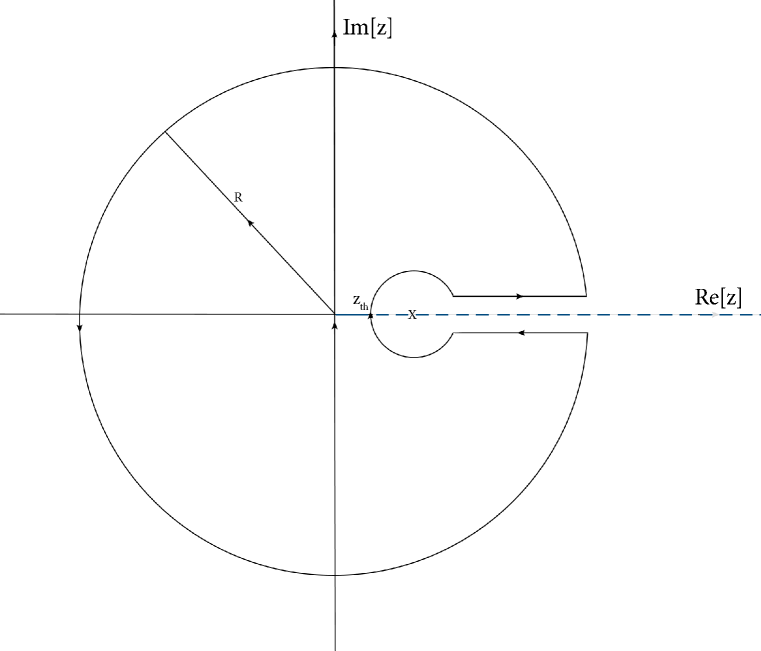
Figure 1: Integration contour used for correlator. X indicates a pole and the broken line indicates a branch cut in the complex plane along the positive real axis corresponding to the resonances

We will also introduce a kernel $\Delta(z)$ which is an arbitrary complete(the zeroth and first order terms are included) quadratic polynomial of $z$. We introduce $\Delta(z)$ to reduce the systematic uncertainties which are associated to the resonances, by constraining $\Delta(z)=0$ at the two resonance peaks. This fixes for us the coefficients of the kernel uniquely.

$$\psi_{5}\left({z_{0}}\right)\Delta\left({z_{0}}\right)$$

$$=\frac{1}{{2\pi i}}\mathop{\oint\mkern-0.8mu}\limits_{C}{\frac{{\psi_{5}\left(z\right)\Delta\left(z\right)}}{{z-z_{0}}}dz}$$

$$=\mathop{\lim}\limits_{\varepsilon\to 0}\frac{1}{{2\pi i}}\int\limits_{z_{th}}^{R}{\frac{{\psi_{5}\left({z+i\varepsilon}\right)\Delta\left({z+i\varepsilon}\right)}}{{z-z_{0}}}dz}+\frac{1}{{2\pi i}}\mathop{\oint\mkern-0.8mu}\limits_{C\left(R\right)}{\frac{{\psi_{5}\left(z\right)\Delta\left(z\right)}}{{z-z_{0}}}dz}+\mathop{\lim}\limits_{\varepsilon\to 0}\frac{1}{{2\pi i}}\int\limits_{R}^{z_{th}}{\frac{{\psi_{5}\left({z-i\varepsilon}\right)\Delta\left({z-i\varepsilon}\right)}}{{z-z_{0}}}dz}$$

$$=\frac{1}{{2\pi i}}\mathop{\oint\mkern-0.8mu}\limits_{C\left(R\right)}{\frac{{\psi_{5}\left(z\right)\Delta\left(z\right)}}{{z-z_{0}}}dz}+\mathop{\lim}\limits_{\varepsilon\to 0}\frac{1}{{2\pi i}}\int\limits_{z_{th}}^{R}{\frac{{\psi_{5}\left({z+i\varepsilon}\right)\Delta\left({z+i\varepsilon}\right)}}{{z-z_{0}}}dz}-\mathop{\lim}\limits_{\varepsilon\to 0}\frac{1}{{2\pi i}}\int\limits_{z_{th}}^{R}{\frac{{\psi_{5}\left({z-i\varepsilon}\right)\Delta\left({z-i\varepsilon}\right)}}{{z-z_{0}}}dz}$$

$$=\frac{1}{{2\pi i}}\mathop{\oint\mkern-0.8mu}\limits_{C\left(R\right)}{\frac{{\psi_{5}\left(z\right)\Delta\left(z\right)}}{{z-z_{0}}}dz}+\mathop{\lim}\limits_{\varepsilon\to 0}\frac{1}{{2\pi i}}\int\limits_{z_{th}}^{R}{\frac{{\psi_{5}\left({z+i\varepsilon}\right)\Delta\left({z+i\varepsilon}\right)-\psi_{5}\left({z-i\varepsilon}\right)\Delta\left({z-i\varepsilon}\right)}}{{z-z_{0}}}dz}$$ (3.2)

The residue from the pole is included in the hadronic spectral function. Since $\Delta(z)$ is a single valued analytic function, in the limit

$$\mathop{\lim}\limits_{\varepsilon\to 0}\Delta\left({z+i\varepsilon}\right)=\mathop{\lim}\limits_{\varepsilon\to 0}\Delta\left({z-i\varepsilon}\right)=\Delta\left(z\right)$$

${\psi_{5}\left({z+i\varepsilon}\right)}$ and ${\psi_{5}\left({z-i\varepsilon}\right)}$ are the functions evaluated in the two different branches or Riemann sheets of the function and we have that

$$\mathop{\lim}\limits_{\varepsilon\to 0}\psi_{5}\left({z+i\varepsilon}\right)\neq\mathop{\lim}\limits_{\varepsilon\to 0}\psi_{5}\left({z-i\varepsilon}\right)$$

we can now write the (3.2) as

$$\psi_{5}\left({z_{0}}\right)\Delta\left({z_{0}}\right)=\frac{1}{{2\pi i}}\mathop{\oint\mkern-0.8mu}\limits_{C\left(R\right)}{\frac{{\psi_{5}\left(z\right)\Delta\left(z\right)}}{{z-z_{0}}}dz}+\frac{1}{{2\pi i}}\int\limits_{z_{th}}^{R}{\frac{{\Delta\left(z\right)}}{{z-z_{0}}}\mathop{\lim}\limits_{\varepsilon\to 0}\left[{\psi_{5}\left({z+i\varepsilon}\right)-\psi_{5}\left({z-i\varepsilon}\right)}\right]dz}$$ (3.3)

let us now consider an analytic function $f(z+i\varepsilon)$, we can Laurent expand this function around $z$ as

$$f\left({z+i\varepsilon}\right)=\sum\limits_{n=0}^{\infty}{\frac{{f^{\left(n\right)}\left({i\varepsilon}\right)}}{{n!}}z^{n}}$$ (3.4)

were $f^{\left(n\right)}\left({i\varepsilon}\right)$ is the n^th derivative of the function $f(z)$ evaluated at the point $z=i\varepsilon$. We can do the same for the function $f(z-i\varepsilon)$ which is

$$f\left({z-i\varepsilon}\right)=\sum\limits_{n=0}^{\infty}{\frac{{f^{\left(n\right)}\left({-i\varepsilon}\right)}}{{n!}}z^{n}}$$ (3.5)

We can now evaluate the difference of these functions

$$f\left({z+i\varepsilon}\right)-f\left({z-i\varepsilon}\right) = \sum\limits_{n=0}^{\infty}{\frac{{f^{\left(n\right)}\left({i\varepsilon}\right)}}{{n!}}z^{n}}-\sum\limits_{n=0}^{\infty}{\frac{{f^{\left(n\right)}\left({-i\varepsilon}\right)}}{{n!}}z^{n}}$$

$$= \sum\limits_{n=0}^{\infty}{\frac{{z^{n}}}{{n!}}}\left[{f^{\left(n\right)}\left({i\varepsilon}\right)-f^{\left(n\right)}\left({-i\varepsilon}\right)}\right]$$

$$= \sum\limits_{n=0}^{\infty}{\frac{{z^{n}}}{{n!}}}\frac{{d^{n}}}{{dz^{n}}}\left[{\left.{f\left(z\right)}\right|_{z=i\varepsilon}-\left.{f\left(z\right)}\right|_{z=-i\varepsilon}}\right]$$

$$= \sum\limits_{n=0}^{\infty}{\frac{{z^{n}}}{{n!}}\frac{{d^{n}}}{{dz^{n}}}\left.{\left[{f\left(z\right)-f\left({\bar{z}}\right)}\right]}\right|_{z=i\varepsilon}}$$

$$= \sum\limits_{n=0}^{\infty}{\frac{{z^{n}}}{{n!}}\frac{{d^{n}}}{{dz^{n}}}\left.{\left[{f\left(z\right)-\overline{f\left(z\right)}}\right]}\right|_{z=i\varepsilon}}$$

$$= \sum\limits_{n=0}^{\infty}{\frac{{z^{n}}}{{n!}}\frac{{d^{n}}}{{dz^{n}}}\left.{2i\operatorname{Im}\left[{f\left(z\right)}\right]}\right|_{z=i\varepsilon}}$$

$$= 2i\operatorname{Im}\left[{\sum\limits_{n=0}^{\infty}{\frac{{z^{n}}}{{n!}}\left.{\frac{{d^{n}}}{{dz^{n}}}f\left(z\right)}\right|_{z=i\varepsilon}}}\right]$$

$$= 2i\operatorname{Im}\left[{\sum\limits_{n=0}^{\infty}{\frac{{z^{n}}}{{n!}}f^{\left(n\right)}\left({i\varepsilon}\right)}}\right]$$

$$= 2i\operatorname{Im}\left[{f\left({z+i\varepsilon}\right)}\right]$$ (3.7)

We have used the Schwartz Reflection Principle [13, 14, 15] in (3) to analytically continue the correlator onto the other side of the branch cut. We now take the limit $\varepsilon\Rightarrow 0$ to obtain

$$\mathop{\lim}\limits_{\varepsilon\to 0}\left[{f\left({z+i\varepsilon}\right)-f\left({z-i\varepsilon}\right)}\right]=\mathop{\lim}\limits_{\varepsilon\to 0}2i\operatorname{Im}\left[{f\left({z+i\varepsilon}\right)}\right]=2i\operatorname{Im}\left[{f\left(z\right)}\right]$$ (3.8)

Now analogously we can do the same for the $\psi_{5}(z)$ to get

$$\mathop{\lim}\limits_{\varepsilon\to 0}\left[{\psi_{5}\left({z+i\varepsilon}\right)-\psi_{5}\left({z-i\varepsilon}\right)}\right]=2i\operatorname{Im}\left[{\psi_{5}\left(z\right)}\right]$$ (3.9)

and substituting (3.9) into (3.3) we obtain

$$\psi_{5}\left({z_{0}}\right)\Delta\left({z_{0}}\right)=\frac{1}{{2\pi i}}\mathop{\oint\mkern-0.8mu}\limits_{C\left(R\right)}{\frac{{\psi_{5}\left(z\right)\Delta\left(z\right)}}{{z-z_{0}}}dz}+\frac{1}{\pi}\int\limits_{z_{th}}^{R}{\frac{{\Delta\left(z\right)}}{{z-z_{0}}}\operatorname{Im}\left[{\psi_{5}\left(z\right)}\right]dz}$$

and in the low energy limit we get

$$\psi_{5}\left(0\right)\Delta\left(0\right)=\frac{1}{{2\pi i}}\mathop{\oint\mkern-0.8mu}\limits_{C\left(R\right)}{\frac{{\Delta\left(z\right)}}{z}\psi_{5}\left(z\right)dz}+\frac{1}{\pi}\int\limits_{z_{th}}^{R}{\frac{{\Delta\left(z\right)}}{z}\operatorname{Im}\left[{\psi_{5}\left(z\right)}\right]dz}$$ (3.10)

Equation (3.10) is referred to as the Finite Energy Sum Rule. The size of the radius of the circle used in the contour integration in (3.10) hints to us which correlating function will be used, if we choose the radius to be large enough then we can use the Perturbative QCD (pQCD) correlator for high energies for $\psi_{5}(z)$ in the contour integral on the circle [16, 17]. For the second term in (3.10) we shall use the Hadronic spectral function.

$$\psi_{5}\left(0\right)\Delta\left(0\right)=\frac{1}{{2\pi i}}\mathop{\oint\mkern-0.8mu}\limits_{C\left(R\right)}{\frac{{\Delta\left(z\right)}}{z}\left.{\psi_{5}\left(z\right)}\right|_{PQCD}dz}+\frac{1}{\pi}\int\limits_{z_{th}}^{R}{\frac{{\Delta\left(z\right)}}{z}\left.{\operatorname{Im}\left[{\psi_{5}\left(z\right)}\right]}\right|_{HAD}dz}$$ (3.11)

For the case of the pion, the hadronic spectral function is the sum of the pion pole term and the resonance terms i.e.

$$\frac{1}{\pi}\left.{\operatorname{Im}\left[{\psi_{5}\left(z\right)}\right]}\right|_{HAD}=2f_{\pi}^{2}M_{\pi}^{4}\delta\left({z-M_{\pi}^{2}}\right)+\frac{1}{\pi}\left.{\operatorname{Im}\left[{\psi_{5}\left(z\right)}\right]}\right|_{RES}$$ (3.12)

substituting (3.12) into the sum rule (3.11) to get

$$\psi_{5}\left(0\right)\Delta\left(0\right)=2f_{\pi}^{2}M_{\pi}^{2}\Delta\left({M_{\pi}^{2}}\right)+\frac{1}{\pi}\int\limits_{z_{th}}^{R}{\frac{1}{z}\Delta\left(z\right)\left.{\operatorname{Im}\left[{\psi_{5}\left(z\right)}\right]}\right|_{RES}dz}+\frac{1}{{2\pi i}}\mathop{\oint\mkern-0.8mu}\limits_{C\left(R\right)}{\frac{1}{z}\Delta\left(z\right)\left.{\psi_{5}\left(z\right)}\right|_{PQCD}dz}$$ (3.13)

For convenience we define two new functions to simplify the work

$$\left.{\delta_{5}\left(R\right)}\right|_{RES} \equiv \frac{1}{\pi}\int\limits_{z_{th}}^{R}{\frac{1}{z}\Delta\left(z\right)\left.{\operatorname{Im}\left[{\psi_{5}\left(z\right)}\right]}\right|_{RES}dz}$$ (3.14)

$$\left.{\delta_{5}\left(R\right)}\right|_{PQCD} \equiv \frac{1}{{2\pi i}}\mathop{\oint\mkern-0.8mu}\limits_{C\left(R\right)}{\frac{1}{z}\Delta\left(z\right)\left.{\psi_{5}\left(z\right)}\right|_{PQCD}dz}$$ (3.15)

the FESR which we will use in the subsequent analysis is then

$$\psi_{5}\left(0\right)\Delta\left(0\right)=2f_{\pi}^{2}M_{\pi}^{2}\Delta\left({M_{\pi}^{2}}\right)+\left.{\delta_{5}\left(R\right)}\right|_{RES}+\left.{\delta_{5}\left(R\right)}\right|_{PQCD}$$ (3.16)

4 Integration in the Complex Plane

We will use three methods to evaluate the $\left.{\delta_{5}\left(R\right)}\right|_{PQCD}$ of (3.15). We will use the method of Fixed Order Perturbation Theory (FOPT) and the method of Fixed Renormalization Scale/Frozen Order Perturbation Theory (FSPT).

The corresponding Perturbative QCD expression for (3.15) can be improved with the help of the Renormalization Group (RG) improvement. In the course of calculating (3.15) we will also need to perform the contour integration over the circle. We now have a choice of which order the integral and the renormalization group improvement will be performed.

4.1 Fixed Order Perturbation Theory

Fixed Order Perturbation Theory [18, 19, 20, 21] refers to first evaluating the contour integral and then performing the renormalization group improvement. The integrals are performed in the complex energy squared plane (z-plane) on a contour which is a circle with fixed energy (constant radius). Since the strong coupling $\alpha_{s}\left(z\right)$ and the masses of the quarks $m_{q}\left(z\right)$ depend only on the magnitude of the complex variable $z$ i.e. depend only on $R$ which is the squared energy in the complex plane, these quantities can be taken out of the contour integral. Only after the integrals are done, we then implement the renormalization group improvement by setting the renormalization scale equal to the radius of the circle i.e. $\mu^{2}=R$, so that all the logarithmic terms in the form $\ln(R/\mu^{2})$ vanish.

The Perturbative QCD correlator given in [19, 22, 23, 24, 25, 26] is

$$\left.{\psi_{5}\left({q^{2}}\right)}\right|_{PQCD}=m_{q}^{2}\left({\left|q\right|^{2}}\right)\left[{-q^{2}\Pi_{0}\left({q^{2}}\right)+m_{q}\left({\left|q\right|^{2}}\right)\Pi_{2}\left({q^{2}}\right)+\frac{{C_{u}}}{{-q^{2}}}\left.{\left\langle{m_{q}\bar{u}u}\right\rangle}\right|_{\mu_{0}}+\sum\limits_{j=1}^{3}{\frac{{C_{j}}}{{-q^{2}}}\left\langle{\hat{O}_{j}}\right\rangle}+\ldots}\right]$$ (4.1.1)

were $\mu_{0}$ is the scale at which the condensate is measured.

$$\Pi_{0}\left({q^{2}}\right) = \frac{1}{{16\pi^{2}}}\left[{-12+6\ln\left({\frac{{-q^{2}}}{{\mu^{2}}}}\right)+\left({\frac{{\alpha_{s}\left({\left|q\right|^{2}}\right)}}{\pi}}\right)\left({24\zeta\left(3\right)-\frac{{131}}{2}+34\ln\left({\frac{{-q^{2}}}{{\mu^{2}}}}\right)-6\ln^{2}\left({\frac{{-q^{2}}}{{\mu^{2}}}}\right)}\right)}\right]$$ (4.1.2)

$$+ \frac{1}{{16\pi^{2}}}\left({\frac{{\alpha_{s}\left({\left|q\right|^{2}}\right)}}{\pi}}\right)^{2}\left[{{\text{A}_{3}}\ln\left({\frac{{-q^{2}}}{{\mu^{2}}}}\right)+{\text{B}_{3}}\ln^{2}\left({\frac{{-q^{2}}}{{\mu^{2}}}}\right)+{\text{C}_{3}}\ln^{3}\left({\frac{{-q^{2}}}{{\mu^{2}}}}\right)}\right]$$

$$+ \frac{1}{{16\pi^{2}}}\left({\frac{{\alpha_{s}\left({\left|q\right|^{2}}\right)}}{\pi}}\right)^{3}\left[{A\ln\left({\frac{{-q^{2}}}{{\mu^{2}}}}\right)+B\ln^{2}\left({\frac{{-q^{2}}}{{\mu^{2}}}}\right)+C\ln^{3}\left({\frac{{-q^{2}}}{{\mu^{2}}}}\right)+D\ln^{4}\left({\frac{{-q^{2}}}{{\mu^{2}}}}\right)}\right]$$

$$+ \frac{1}{{16\pi^{2}}}\left({\frac{{\alpha_{s}\left({\left|q\right|^{2}}\right)}}{\pi}}\right)^{4}\sum\limits_{i=1}^{5}{H_{i}L^{i}}$$

with $H_{i}$ are a set of real numbers and $L^{i}=\rm{ln^{i}}(-q^{2}/\mu^{2})$ and

$$\Pi_{2}\left({q^{2}}\right)=\frac{1}{{16\pi^{2}}}\left\{{-12+12\ln\left({\frac{{-q^{2}}}{{\mu^{2}}}}\right)+\frac{{\alpha_{s}\left({\left|{q^{2}}\right|}\right)}}{\pi}\left[{-1000+64\ln\left({\frac{{-q^{2}}}{{\mu^{2}}}}\right)-24\left[{\ln\left({\frac{{-q^{2}}}{{\mu^{2}}}}\right)}\right]^{2}+48\zeta\left(3\right)}\right]}\right\}$$ (4.1.3)

substituting (4.1.2) and (4.1.3) into (4.1.1) and using $\Delta\left(z\right)=1-a_{0}z-a_{1}z^{2}$ as the integration kernel in (3.15) we obtain

$$\left.{\delta_{5}\left(R\right)}\right|_{PQCD}=\left.{\delta_{5}\left(R\right)}\right|_{\Pi_{0}}+\left.{\delta_{5}\left(R\right)}\right|_{\Pi_{2}}+\left.{\delta_{5}\left(R\right)}\right|_{C_{u}}+\left.{\delta_{5}\left(R\right)}\right|_{C_{j}}$$ (4.1.4)

with

$$\left.{\delta_{5}\left(R\right)}\right|_{\Pi_{0}}=\left.{\delta_{5}}\right|_{1{\text{loop}}}+\left.{\delta_{5}}\right|_{{\text{2loop}}}+\left.{\delta_{5}}\right|_{{\text{3loop}}}+\left.{\delta_{5}}\right|_{{\text{4loop}}}+\left.{\delta_{5}}\right|_{{\text{5loop}}}$$ (4.1.5)

See explicit forms of these functions which have been calculated in the Appendix B.

With the definitions given below we can calculate numerically the behavior of $\left.{\delta_{5}\left(R\right)}\right|_{PQCD}$ as a function of the energy $R$.

The coefficients of the QCD Beta function [25] series for $n$ quark types:

$$\beta_{0} = 0.25\left({11-\frac{2}{3}n}\right)$$

$$\beta_{1} = \frac{1}{{16}}\left({102.0-\frac{{38}}{3}n}\right)$$

$$\beta_{2} = \frac{1}{{64}}\left({\frac{{2857.0}}{2}-\frac{{5033}}{{18}}n+\frac{{325}}{{54}}n^{2}}\right)$$

$$\beta_{3} = \frac{1}{{256.0}}\left({\frac{{149753}}{{6.0}}+3564\zeta(3)-\left({\frac{{1078361}}{{162.0}}+\frac{{6508}}{{27}}\zeta(3)}\right)n+\left({\frac{{50065}}{{162.0}}+\frac{{6472}}{{81}}\zeta(3)}\right)n^{2}+\frac{{1093}}{{729.0}}n^{3}}\right)$$

$\Lambda\equiv\Lambda_{\rm{QCD}}$ for the definitions found in [19, 26]:

$$L[z,\Lambda] = \ln\left[{\frac{z}{{\Lambda^{2}}}}\right]$$

$$a1[z,\Lambda] = -\frac{{\beta_{1}}}{{\beta_{0}^{2}}}\ln[L[z,\Lambda]]$$

$$a2[z,\Lambda] = \frac{1}{{\beta_{0}^{2}}}\left({\frac{{\beta_{1}^{2}}}{{\beta_{0}^{2}}}\left({\ln[L[z,\Lambda]]^{2}-\ln[L[z,\Lambda]]-1}\right)+\frac{{\beta_{2}}}{{\beta_{0}}}}\right)$$

$$a3[z,\Lambda] = \frac{1}{{\beta_{0}^{3}}}\left({\frac{{\beta_{1}^{3}}}{{\beta_{0}^{3}}}\left({-\ln[L[z,\Lambda]]^{3}+2.5\ln[L[z,\Lambda]]^{2}+2\ln[L[z,\Lambda]]-0.5}\right)-3\frac{{\beta_{1}\beta_{2}}}{{\beta_{0}^{2}}}\ln[L[z,\Lambda]]+0.5\frac{{\beta_{3}}}{{\beta_{0}}}}\right)$$

$$\alpha[z,\Lambda] = \frac{\pi}{{\beta_{0}L[z,\Lambda]}}\left({1+\frac{{a1[z,\Lambda]}}{{L[z,\Lambda]}}+\frac{{a2[z,\Lambda]}}{{L[z,\Lambda]^{2}}}+\frac{{a3[z,\Lambda]}}{{L[z,\Lambda]^{3}}}}\right)$$ (4.1.6)

The coefficients of the QCD Gamma function series for quark masses:

$$\gamma_{0} = 1$$

$$\gamma_{1} = \frac{1}{{16}}\left({\frac{{202}}{3}-\frac{{20}}{9}n}\right)$$

$$\gamma_{2} = \frac{1}{{64}}\left[{1249.0-\left({\frac{{2216}}{{27.0}}+\frac{{160}}{3}\zeta\left(3\right)}\right)n-\frac{{140}}{{81.0}}n^{2}}\right]$$

$$\gamma_{3} = \frac{1}{{256}}\left[{\left({\frac{{4603055}}{{162.0}}+\frac{{135680}}{{27}}\zeta\left(3\right)-8800\zeta\left(5\right)}\right)+\left({-\frac{{91723}}{{27}}-\frac{{34192}}{9}\zeta\left(3\right)+880\zeta\left(4\right)+\frac{{18400}}{9}\zeta\left(5\right)}\right)n}\right]$$

$$+ \frac{1}{{256}}\left[{\left({\frac{{5242}}{{243}}+\frac{{800}}{9}\zeta\left(3\right)-\frac{{160}}{3}\zeta\left(3\right)}\right)n^{2}+\left({-\frac{{332}}{{243}}+\frac{{64}}{{27}}\zeta\left(3\right)}\right)n^{3}}\right]$$

$$d1[z,\Lambda] = -\frac{{\gamma_{0}\beta_{1}}}{{\beta_{0}^{3}}}{\text{ln}}[L[z,\Lambda]]$$

$$d2[z,\Lambda] = \frac{{\gamma_{0}}}{{\beta_{0}^{3}}}\left({\frac{\beta_{1}^{2}}{{\beta_{0}^{2}}}\left({{\text{ln}}[L[z,\Lambda]]^{2}-{\text{ln}}[L[z,\Lambda]]-1}\right)+\frac{\beta_{2}}{{\beta_{0}}}}\right)+0.5\frac{{\gamma_{0}}}{{\beta_{0}}}\left({\frac{{\gamma_{0}}}{{\beta_{0}}}-1}\right)\frac{{{\beta_{1}}^{2}}}{{\beta_{0}^{4}}}{\text{ln}}[L[z,\Lambda]]^{2}$$

$$d3[z,\Lambda] = \frac{{\gamma_{0}}}{{\beta_{0}^{4}}}\left({\frac{{{\beta_{1}}^{3}}}{{\beta_{0}^{3}}}\left({-{\text{ln}}[L[z,\Lambda]]^{3}+2.5{\text{ln}}[L[z,\Lambda]]^{2}+2{\text{ln}}[L[z,\Lambda]]-0.5}\right)-3\frac{{\beta_{1}\beta_{2}}}{{\beta_{0}^{2}}}{\text{ln}}[L[z,\Lambda]]+0.5\frac{{\beta_{3}}}{{\beta_{0}}}}\right)$$

$$+ 0.5\frac{{\gamma_{0}}}{{\beta_{0}}}\left({\frac{{\gamma_{0}}}{{\beta_{0}}}-1}\right)\left({-2\frac{{\beta_{1}}}{{\beta_{0}^{4}}}}\right)\left({\frac{{\beta_{1}^{2}}}{{\beta_{0}^{2}}}\left({{\text{ln}}[L[z,\Lambda]]^{2}-{\text{ln}}[L[z,\Lambda]]-1}\right)+\frac{{\beta_{2}}}{{\beta_{0}}}}\right){\text{ln}}[L[z,\Lambda]]$$

$$- \frac{1}{6}\frac{{\gamma_{0}}}{{\beta_{0}}}\left({\frac{{\gamma_{0}}}{{\beta_{0}}}-1}\right)\left({\frac{{\gamma_{0}}}{{\beta_{0}}}-2}\right)\frac{{\beta_{1}^{3}}}{{\beta_{0}^{6}}}{\text{ln}}[L[z,\Lambda]]^{3}$$

$$c1 = \frac{{\gamma_{1}}}{{\beta_{0}}}-\frac{{\gamma_{0}\beta_{1}}}{{\beta_{0}^{2}}}$$

$$c2 = 0.5\left({\frac{{\gamma_{2}}}{{\beta_{0}}}-\frac{{\gamma_{1}\beta_{1}}}{{\beta_{0}^{2}}}+\frac{{\gamma_{0}}}{{\beta_{0}^{2}}}\left({\frac{{\beta_{1}^{2}}}{{\beta_{0}}}-\beta_{2}}\right)}\right)$$

$$c3 = \frac{1}{3}\left({\frac{{\gamma_{0}}}{{\beta_{0}^{2}}}\left({\frac{{\beta_{1}\beta_{2}}}{{\beta_{0}}}-\frac{{\beta_{1}}}{{\beta_{0}}}\left({\frac{{\beta_{1}^{2}}}{{\beta_{0}}}-\beta_{2}}\right)-\beta_{3}}\right)+\frac{{\gamma_{1}}}{{\beta_{0}^{2}}}\left({\frac{{\beta_{1}^{2}}}{{\beta_{0}}}-\beta_{2}}\right)-\frac{{\beta_{1}\gamma_{2}}}{{\beta_{0}^{2}}}+\frac{{\gamma_{3}}}{{\beta_{0}}}}\right)$$

For convenience we have split the right-hand-side of the quark mass function into a product of the invariant quark mass $\widehat{m}_{\Lambda}$ and the functional dependence on the energy $z$ and the $\Lambda_{\rm{QCD}}$ scale in the $U\left({z,\Lambda}\right)$

$$U\left({z,\Lambda}\right)= \frac{1}{{\left({\frac{1}{2}L\left[{z,\Lambda}\right]}\right)^{\frac{{\gamma_{0}}}{{\beta_{0}}}}}}\Biggl{\{}1+\left({\frac{{c1}}{{\beta_{0}}}+d1\left[{z,\Lambda}\right]}\right)\frac{1}{{L[z,\Lambda]}}+$$

$$+\left[{\left({c1\frac{{a1\left[{z,\Lambda}\right]}}{{\beta_{0}}}+\frac{{0.5c1^{2}+c2}}{{\beta_{0}^{2}}}}\right)+d2\left[{z,\Lambda}\right]+c1\frac{{d1\left[{z,\Lambda}\right]}}{{\beta_{0}}}}\right]\frac{1}{{L\left[{z,\Lambda}\right]^{2}}}$$

$$+ \left[{c1\frac{{a2\left[{z,\Lambda}\right]}}{{\beta_{0}}}+\frac{{\left({c2+0.5c1^{2}}\right)}}{{\beta_{0}^{2}}}\left({d1\left[{z,\Lambda}\right]-2\frac{{\beta_{1}}}{{\beta_{0}^{2}}}\ln\left[{L\left[{z,\Lambda}\right]}\right]}\right)+\frac{{c3+c1c2+\frac{1}{6}c1^{3}}}{{\beta_{0}^{3}}}}\right]\frac{1}{{L\left[{z,\Lambda}\right]^{3}}}$$

$$+ \left[{c1\frac{{d1\left[{z,\Lambda}\right]a1\left[{z,\Lambda}\right]}}{{\beta_{0}}}+c1\frac{{d2\left[{z,\Lambda}\right]}}{{\beta_{0}}}+d3\left[{z,\Lambda}\right]}\right]\frac{1}{{L\left[{z,\Lambda}\right]^{3}}}\Biggr{\}}$$ (4.1.7)

were

$$m\left({z,\Lambda}\right)=\widehat{m}_{\Lambda}U\left({z,\Lambda}\right)$$ (4.1.8)

4.2 Fixed Renormalization Scale Perturbation Theory

The method of Fixed Renormalization Scale Perturbation Theory [27, 28, 29] is very similar to the method of Fixed Order Perturbation Theory. In this case we generalize the integration kernel from a simply second order polynomial to a $n^{th}$ order polynomial and instead of choosing the renormalization scale to be radius of the circle in the complex energy plane we will instead choose a fixed scale which will be varied over a large interval of $\mu^{2}=2-50$ GeV². The method is implemented by using the Legendre polynomials [30] and making use of their orthogonality property. We first generalize the kernel to

$$\tilde{\Delta}_{n}\left(z\right)\equiv\frac{{P_{n}\left[{x\left(z\right)}\right]}}{{P_{n}\left[{x\left({M_{\pi}^{2}}\right)}\right]}}=\sum\limits_{j=0}^{n}{a_{j}z^{j}}$$ (4.2.1)

were $P_{n}$ is the Legendre polynomial which can be generated by the Rodriguez Formula

$$P_{n}\left(x\right)=\frac{1}{{2^{n}n!}}\left({\frac{d}{{dx}}}\right)^{n}\left({x^{2}-1}\right)^{n}$$ (4.2.2)

We use the orthogonality of the polynomials i.e.

$$\int\limits_{-1}^{1}{P_{n}\left(x\right)P_{m}\left(x\right)dx}=0$$

for $n\neq m$ by rescaling the domain of integration as

$$x\left(z\right)\equiv\frac{{2z-\left({z_{0}-z_{th}}\right)}}{{z_{th}-z_{0}}}$$

with $z\in\left[{z_{th};z_{0}}\right]$ yields the following constraints on (4.2.1)

$$\tilde{\Delta}_{n}\left({M_{\pi}^{2}}\right) = 1$$ (4.2.3)

$$\int\limits_{z_{th}}^{z_{0}}{z^{k}\tilde{\Delta}_{n}\left(z\right)dz} = 0{\text{ }}k\in\mathbb{N},k<n$$ (4.2.4)

Imposing the orthogonality condition (4.2.4) forces the generalized polynomial $\tilde{\Delta}_{n}\left(z\right)$ to minimize the contributions of the continuum in the range $z\in\left[{z_{th};z_{0}}\right]$.

We then substitute (4.2.1) into (3.15) and (3.14) and choose allow $\mu^{2}$ to vary in the range $2-50$ GeV². In our case we found the best(largest stable domain) results for $\mu^{2}=4$ GeV². We varied the value of $\mu^{2}$ in the range $2-50$ GeV² to obtain an uncertainty in the value of the $\delta_{\pi}$

5 The Resonance Contribution $\left.{\delta_{5}\left(R\right)}\right|_{RES}$

To evaluate the resonance term (3.14) we require information about the hadronic spectral function beyond the pion pole. At the current time this information is not available from experiment and we only have information about the mass and width of the first two excited states of the pion i.e. the $\Pi(1300)$ [31] and the $\Pi(1800)$ excitations. To proceed further we shall have to model the hadronic spectral function by using threshold constraints from Chiral Perturbation Theory ($\chi$-PT) which are imposed on a linear combination of Breit-Wigner profiles to describe the two excitations of the pion. Alas by introducing this model we will also introduce systematic uncertainties and solutions obtained thereafter are dependent on the model used. However, we can reduce these systematic uncertainties by introducing analytic integration kernels that are forced to be zero at the resonance points. This will reduce the effect of the systematic uncertainties in the neighborhood of the resonances. We have introduced the quadratic polynomial $\Delta(z)$ earlier precisely because of this!

We shall start by modeling the hadronic spectral function as

$$\frac{1}{\pi}\left.{\operatorname{Im}\left[{\psi_{5}\left(z\right)}\right]}\right|_{RES}=\frac{1}{\pi}\left.{\operatorname{Im}\left[{\psi_{5}\left(z\right)}\right]}\right|_{3\pi}BW\left(z\right)$$ (5.1)

were

$$\frac{1}{\pi}\left.{\operatorname{Im}\left[{\psi_{5}\left(z\right)}\right]}\right|_{3\pi}=\frac{1}{{3\cdot 2^{8}\pi^{4}}}\frac{{M_{\pi}^{4}}}{{f_{\pi}^{2}}}z\Theta\left(z\right)$$ (5.2)

is the constraint from $\chi$-PT [32]. The Breit-Wigner profile BW(z) will be in the form

$$BW\left(z\right)=\frac{{BW_{1}\left(z\right)+\kappa BW_{2}\left(z\right)}}{{1+\kappa}}$$ (5.3)

the $\kappa$ is just a weighting parameter which controls the relative weight of the resonances with $\kappa\in\mathbb{R}^{+}$. $\kappa=0.5$ was chosen for the computational work since the width of the $\Pi(1300)$ is twice as broad as the width of the $\Pi(1812)$ resonance and thus the $\Pi(1812)$ resonance would only contribute half as much as the $\Pi(1300)$ resonance. The $BW_{1}\left(z\right)$ and $BW_{2}\left(z\right)$ are isolated Breit-Wigner resonances. We normalize the Breit-Wigner profile at zero to be $BW(0)=1$, this implies that $BW_{1}(0)=1$ and $BW_{2}(0)=1$. This sets the form of the Breit-Wigner resonances we will have to use

$$BW_{k}\left(z\right)=\frac{{M_{k}^{2}\left({M_{k}^{2}+\Gamma_{k}^{2}}\right)}}{{\left({z-M_{k}^{2}}\right)^{2}+M_{k}^{2}\Gamma_{k}^{2}}}$$ (5.4)

we can now proceed with the calculation, substituting (5.2) and (5.3) into (5.1) we obtain

$$\frac{1}{\pi}\left.{\operatorname{Im}\left[{\psi_{5}\left(z\right)}\right]}\right|_{RES}=\frac{1}{{3\cdot 2^{8}\pi^{4}}}\frac{{M_{\pi}^{4}}}{{f_{\pi}^{2}}}\frac{1}{{1+\kappa}}z\Theta\left(z\right)\left[{BW_{1}\left(z\right)+\kappa BW_{2}\left(z\right)}\right]$$ (5.5)

for convenience we define a new parameter $\lambda$ which is just a collection of all the constants

$$\lambda\equiv\frac{1}{{3\cdot 2^{8}\pi^{4}}}\frac{{M_{\pi}^{4}}}{{f_{\pi}^{2}}}\frac{1}{{1+\kappa}}$$

and

$$\frac{1}{\pi}\left.{\operatorname{Im}\left[{\psi_{5}\left(z\right)}\right]}\right|_{RES}=\lambda z\Theta\left(z\right)\left[{BW_{1}\left(z\right)+\kappa BW_{2}\left(z\right)}\right]$$ (5.6)

we can now calculate the resonance contribution in this model by substituting (5.6) into (3.14) to get

$$\left.{\delta_{5}\left(R\right)}\right|_{RES} = \int\limits_{z_{th}}^{R}{\frac{1}{z}\Delta\left(z\right)\lambda z\Theta\left(z\right)\left[{BW_{1}\left(z\right)+\kappa BW_{2}\left(z\right)}\right]dz}$$ (5.7)

$$= \lambda\int\limits_{9M_{\pi}^{2}}^{R}{\frac{1}{z}\Delta\left(z\right)z\Theta\left(z\right)BW_{1}\left(z\right)dz}+\lambda\kappa\int\limits_{9M_{\pi}^{2}}^{R}{\frac{1}{z}\Delta\left(z\right)z\Theta\left(z\right)BW_{2}\left(z\right)dz}$$

$$= \lambda\left[{G_{1}\left(R\right)-G_{1}\left({9M_{\pi}^{2}}\right)}\right]+\lambda\kappa\left[{G_{2}\left(R\right)-G_{2}\left({9M_{\pi}^{2}}\right)}\right]$$

were the function $G_{k}\left(x\right)$ is

$$G_{k}\left(z\right)=M_{k}^{2}\left({M_{k}^{2}+\Gamma_{k}^{2}}\right)\Biggl{\{}\frac{1}{{M_{k}\Gamma_{k}}} \left[{1-a_{0}M_{k}^{2}-a_{1}\left({M_{k}^{4}-M_{k}^{2}\Gamma_{k}^{2}}\right)}\right]\arctan\left({\frac{{z-M_{k}^{2}}}{{M_{k}\Gamma_{k}}}}\right)+$$

$$-\left({\frac{1}{2}a_{0}+a_{1}M_{k}^{2}}\right)\ln\left[{\left({z-M_{k}^{2}}\right)^{2}+M_{k}^{2}\Gamma_{k}^{2}}\right]-a_{1}\left({z-M_{k}^{2}}\right)\Biggr{\}}$$

which is derived in Appendix G. The inclusion of the analytic integration kernel $\Delta(z)$ attempts to suppress the uncertainties from the resonance regions which is poorly understood. Even with this suppression we cannot eliminate entirely these uncertainties. To get a handle on how good the suppression is we make a Taylor expansion of the $\delta_{5}$ or equivalently the $G_{k}(z)$ around the resonance peak. For convenience we shall choose $k=1$ and keeping only the first order terms in the expansion we obtain to leading order

$$\delta_{5}\left(R\right)\approx\lambda M_{1}^{2}\left({M_{1}^{2}+\Gamma_{1}^{2}}\right)\frac{{M_{1}^{2}-M_{2}^{2}}}{{2M_{1}^{2}M_{2}^{2}}}\left\{{\left({\frac{{R-M_{1}^{2}}}{{M_{1}\Gamma_{1}}}}\right)+\ln\left({M_{1}\Gamma_{1}}\right)^{2}}\right\}$$ (5.9)

The coefficient of the braces is the gradient of this line and sets the size on the contribution from the resonances. The magnitude of this coefficient is

$$\lambda M_{1}^{2}\left({M_{1}^{2}+\Gamma_{1}^{2}}\right)\frac{{M_{1}^{2}-M_{2}^{2}}}{{2M_{1}^{2}M_{2}^{2}}}=1.2\times 10^{-7}$$

We see that not only in the immediate neighborhood ($R\approx M_{1}^{2}$) is the suppression effective but due to the tiny coefficient, the contribution from the resonances is effectively eliminated!

6 Results

We consider two cases,

• $SU(2)\otimes SU(2)$ for the Pions

• $SU(3)\otimes SU(3)$ case for the Kaons

of which the FOPT results will be of main interest.We use the particle data from the Particle Data Group [33, 34] for the $SU(2)\otimes SU(2)$ Pion case

• $m_{\pi}=139.642400\pm 0.00035$ MeV

• $f_{\pi}=92.21\pm 0.14$ MeV

• $m_{\pi}^{*}=1300\pm 100$ MeV

• $\Gamma_{\pi}^{*}=400\pm 200$ MeV

• $m_{\pi}^{**}=1812\pm 14$ MeV

• $\Gamma_{\pi}^{**}=207\pm 13$ MeV

• $\overline{m}_{u}(2\rm{GeV})=2.9\pm 0.2$ MeV

• $\overline{m}_{d}(2\rm{GeV})=5.3\pm 0.4$ MeV

• $\hat{m}_{u}(2\rm{GeV})=3.8-3.9$ MeV

• $\hat{m}_{d}(2\rm{GeV})=6.4-7.2$ MeV

$SU(3)\otimes SU(3)$ Kaon[30, 34] case

• $m_{K}=493.677\pm 0.005$ MeV

• $m_{K}^{*}=1460$ MeV

• $\Gamma_{K}^{*}=250$ MeV

• $m_{K}^{**}=1830$ MeV

• $\Gamma_{K}^{**}=250$ MeV

• $\overline{m}_{u}(2\rm{GeV})=2.9\pm 0.2$ MeV

• $\hat{m}_{u}(2\rm{GeV})=3.8-3.9$ MeV

• $\hat{m}_{s}(2\rm{GeV})=130-150$ MeV

We note here that for the plots presented below we will be searching for the so-called stable region. This is the domain on the plot where the function varies the slowest. This domain then defines the stability region. Once we have identified the stability region we read of the average value of the function over this domain. We shall use either $\Lambda_{\rm{QCD}}=0.365$ GeV or $\Lambda_{\rm{QCD}}=0.397$ GeV. It has become standard practice to make predictions about hadronic parameters at these scales.

6.1 Frozen Order Results

6.1.1 $SU(2)\otimes SU(2)$

Figure 2: Results for $\psi_{5}(0)$(GeV⁴) [30] as a function of the energy $s$ in FSPT with $\mu^{2}=4$GeV². a, b and c correspond to polynomial orders 4, 5 and 6 respectively.

From the Fixed Scale Perturbation Theory we see that the stability is over a small interval instead of the whole integration range. From the stable intervals we extract a value of $\delta_{\pi}=0.056\pm 0.011$

6.2 FOPT Results

6.2.1 $SU(2)\otimes SU(2)$

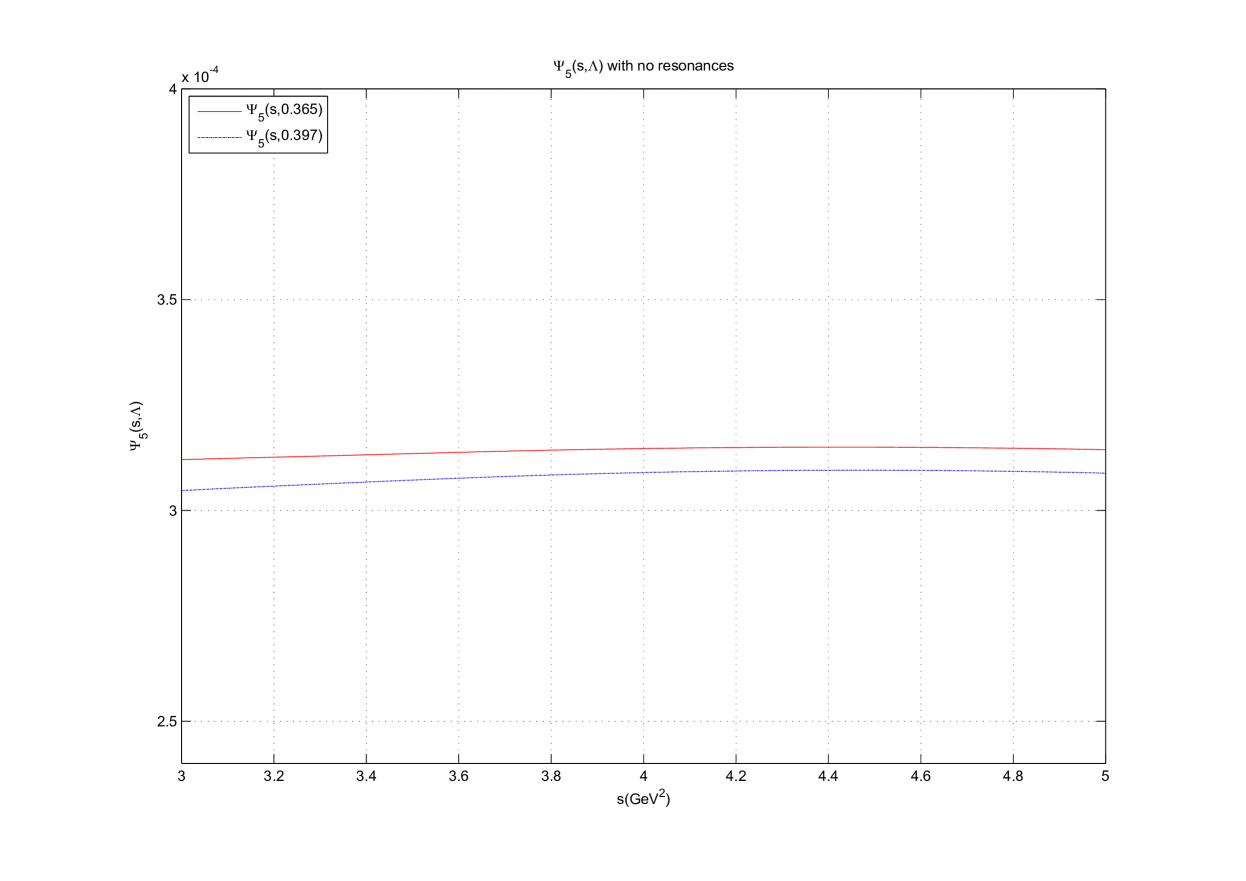
Figure 3: Results for $\psi_{5}(0)$(GeV⁴) as a function of the energy $s$ in FOPT. We have neglected the two resonances. Starting from the top we have $\psi_{5}(s,0.365)$ and $\psi_{5}(s,0.397)$ respectively

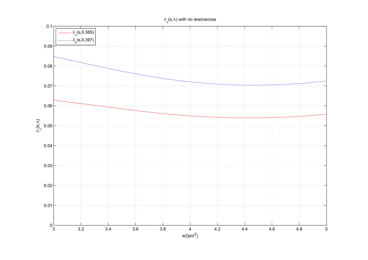
Figure 4: Results for $\delta_{\pi}$ as a function of the energy $s$ in FOPT. We have neglected the two resonances. Starting from the top we have $\delta_{\pi}(s,0.397)$ and $\delta_{\pi}(s,0.365)$ respectively

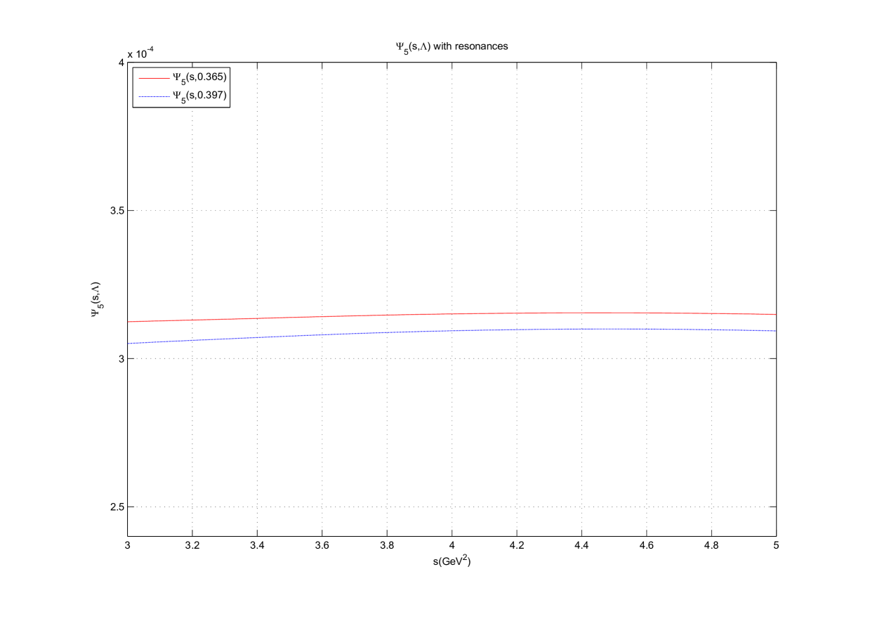
Figure 5: Results for $\psi_{5}(0)$(GeV⁴) as a function of the energy $s$ in FOPT. We have included the two resonances with the weighting factor $\kappa=0.5$. Starting from the top we have $\psi_{5}(s,0.365)$ and $\psi_{5}(s,0.397)$ respectively

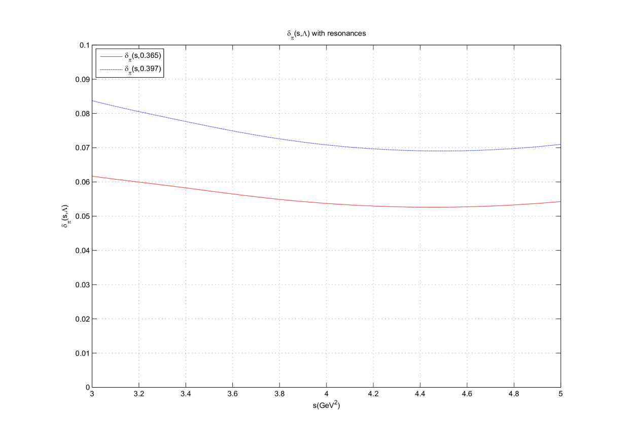
Figure 6: Results for $\delta_{\pi}$ as a function of the energy $s$ in FOPT. We have included the two resonances with the weighting factor $\kappa=0.5$. Starting from the top we have $\delta_{\pi}(s,0.397)$ and $\delta_{\pi}(s,0.365)$ respectively

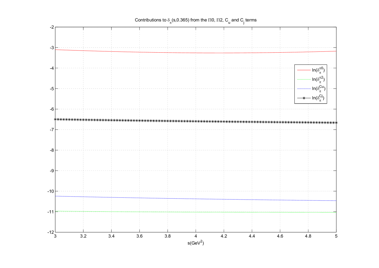
Figure 7: Plot of the various contributors to $\delta_{\pi}$ for $\Lambda_{QCD}=0.365$ GeV. Starting from the top we have $\ln(\delta_{\pi}^{\pi 0})$, $\ln(\delta_{\pi}^{C_{j}})$, $\ln(\delta_{\pi}^{C_{u}})$ and $\ln(\delta_{\pi}^{\pi 2})$ respectively

The various contributions are defined as

$$\psi_{5} = 2f_{\pi}^{2}M_{\pi}^{2}\Delta\left({M_{\pi}^{2}}\right)+\delta_{5PQCD}+\delta_{5RES}$$

$$\delta_{\pi} = 1-\frac{{\psi_{5}}}{{2f_{\pi}^{2}M_{\pi}^{2}}}=1-\frac{{2f_{\pi}^{2}M_{\pi}^{2}\Delta\left({M_{\pi}^{2}}\right)+\delta_{5PQCD}+\delta_{5RES}}}{{2f_{\pi}^{2}M_{\pi}^{2}}}$$ (6.1)

$$= \underbrace{1-\frac{{2f_{\pi}^{2}M_{\pi}^{2}\Delta\left({M_{\pi}^{2}}\right)+\delta_{5RES}}}{{2f_{\pi}^{2}M_{\pi}^{2}}}}_{=\delta_{\pi}^{0}}-\underbrace{\frac{{\left.{\delta_{5}}\right|_{\Pi 0}}}{{2f_{\pi}^{2}M_{\pi}^{2}}}}_{=\delta_{\pi}^{\Pi 0}}-\underbrace{\frac{{\left.{\delta_{5}}\right|_{\Pi 2}}}{{2f_{\pi}^{2}M_{\pi}^{2}}}}_{=\delta_{\pi}^{\Pi 2}}-\underbrace{\frac{{\left.{\delta_{5}}\right|_{Cu}}}{{2f_{\pi}^{2}M_{\pi}^{2}}}}_{=\delta_{\pi}^{Cu}}-\underbrace{\frac{{\left.{\delta_{5}}\right|_{Cj}}}{{2f_{\pi}^{2}M_{\pi}^{2}}}}_{=\delta_{\pi}^{Cj}}$$

$$= \delta_{\pi}^{0}-\delta_{\pi}^{\Pi 0}-\delta_{\pi}^{\Pi 2}-\delta_{\pi}^{Cu}-\delta_{\pi}^{Cj}$$

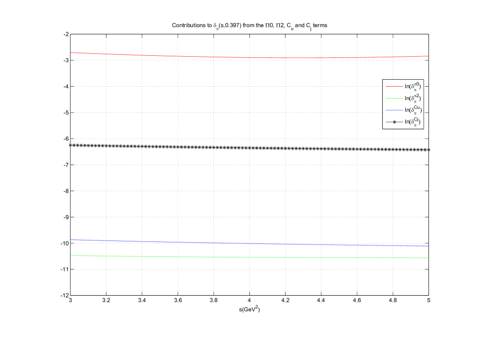
Figure 8: Plot of the various contributors to $\delta_{\pi}$ for $\Lambda_{QCD}=0.397$ GeV. Starting from the top we have $\ln(\delta_{\pi}^{\pi 0})$, $\ln(\delta_{\pi}^{C_{j}})$, $\ln(\delta_{\pi}^{C_{u}})$ and $\ln(\delta_{\pi}^{\pi 2})$ respectively

In the case of FOPT the results show good stability, looking at figures 3 - 5 in the range $3\leq s\leq 5$ $\times 10^{-4}\rm{GeV}^{2}$ there is very little change in $\psi_{5}(s)$ and $\delta_{\pi}(s)$. With the inclusion of the resonances the functions still display good stability. From the data used to generate the above plots, the result are tabulated below

		Pion data
	No Resonances		With Resonances
$\Lambda_{QCD}$(GeV)	$\psi_{5}(0)(\rm{GeV}^{4})\times 10^{-4}$	$\delta_{\pi}$	$\psi_{5}(0)(\rm{GeV}^{4})\times 10^{-4}$	$\delta_{\pi}$
0.365	3.12-3.14	0.059-0.062	3.12-3.16	0.052-0.054
0.397	3.04-3.09	0.072-0.073	3.04-3.09	0.068-0.071

Table 1: Tabulated values extracted from the plots 3 - 5 which are used to estimate $\delta_{\pi}$.

from values listed in table 1, we estimate the value of $\delta_{\pi}=0.064\pm 0.008$.

6.2.2 $SU(3)\otimes SU(3)$

Figure 9: Results for $\psi_{5}(0)$(GeV⁴) as a function of the energy $s$ in FOPT. We have neglected the two resonances. Starting from the top we have $\psi_{5}(s,0.365)$ and $\psi_{5}(s,0.397)$ respectively

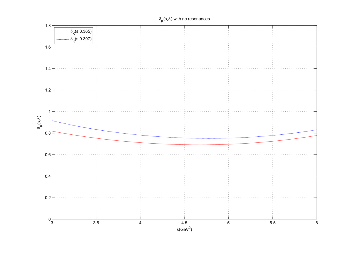
Figure 10: Results for $\delta_{\pi}$ as a function of the energy $s$ in FOPT. We have neglected the two resonances. Starting from the top we have $\delta_{K}(s,0.397)$ and $\delta_{K}(s,0.365)$ respectively

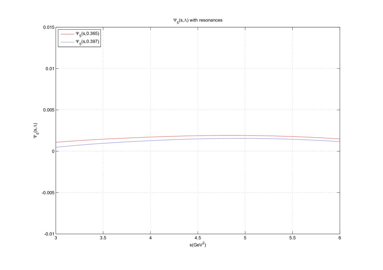
Figure 11: Results for $\psi_{5}(0)$(GeV⁴) as a function of the energy $s$ in FOPT. We have included the two resonances with the weighting factor $\kappa=0.5$. Starting from the top we have $\psi_{5}(s,0.365)$ and $\psi_{5}(s,0.397)$ respectively

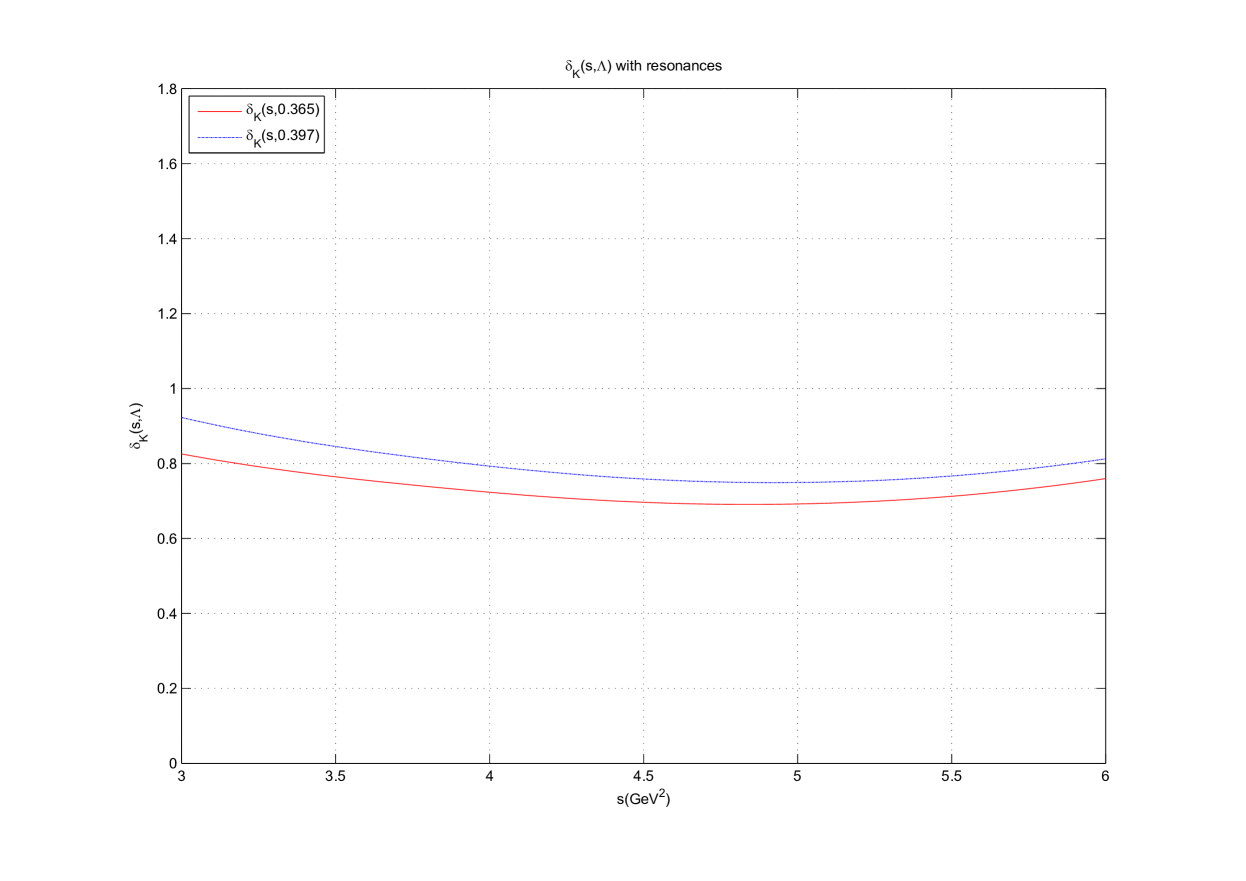
Figure 12: Results for $\delta_{\pi}$ as a function of the energy $s$ in FOPT. We have included the two resonances with the weighting factor $\kappa=0.5$. Starting from the top we have $\delta_{K}(s,0.397)$ and $\delta_{K}(s,0.365)$ respectively

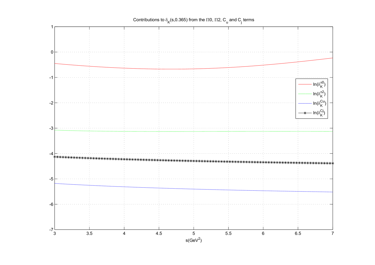
Figure 13: Plot of the various contributors to $\delta_{K}$ for $\Lambda_{QCD}=0.365$ GeV. Starting from the top we have $\ln(\delta_{K}^{\pi 0})$, $\ln(\delta_{K}^{\pi 2})$, $\ln(\delta_{K}^{C_{j}})$ and $\ln(\delta_{K}^{C_{u}})$ respectively

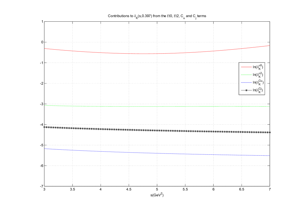
Figure 14: Plot of the various contributors to $\delta_{K}$ for $\Lambda_{QCD}=0.397$ GeV. Starting from the top we have $\ln(\delta_{K}^{\pi 0})$, $\ln(\delta_{K}^{\pi 2})$, $\ln(\delta_{K}^{C_{j}})$ and $\ln(\delta_{K}^{C_{u}})$ respectively

Looking at figures 9 - 12 in the range $4\leq s\leq 5$ $\times 10^{-4}\rm{GeV}^{2}$ there is very little change in $\psi_{5}(s)$ and $\delta_{K}(s)$. With the inclusion of the resonances the functions still display good stability. From the data used to generate the above plots, the result are tabulated below:

Kaon data
	No Resonances		With Resonances
$\Lambda_{QCD}(\rm{GeV})$	$\psi_{5}(0)(\rm{GeV}^{4})$	$\delta_{K}$	$\psi_{5}(0)(\rm{GeV}^{4})$	$\delta_{K}$
0.365	0.0017-0.0019	0.6929-0.6963	0.0018-0.0019	0.6921-0.6959
0.397	0.0013-0.0015	0.7535-0.7542	0.0014-0.0015	0.7493-0.7578

Table 2: Tabulated values extracted from the plots 9 - 12 which are used to estimate $\delta_{K}$.

From values listed in table 2, we estimate the value of $\delta_{K}=0.64\pm 0.24$.

6.3 Discussion of Results

We have estimated the values of the $\delta_{\pi}$ and $\delta_{K}$ as (taking averages and adding the errors in quadrature)

$$\delta_{\pi} = 0.060\pm 0.014$$ (6.1)

$$\delta_{K} = 0.64\pm 0.24$$ (6.2)

The estimated value of $\delta_{\pi}$ is larger than the value estimated in [35] which is based on perturbative QCD up to next-to-leading order. We can use the value for $\delta_{\pi}$ to find the quark condensate by using the current quark mass of $0.5\left({m_{u}+m_{d}}\right)=4.1\pm 0.2$ MeV and substituting into (3.1) to get

$$\left\langle{0|\bar{q}q|0}\right\rangle = -\frac{{f_{\pi}^{2}M_{\pi}^{2}\left({1-\delta_{\pi}}\right)}}{{2\cdot 0.5\left({m_{u}+m_{d}}\right)}}$$ (6.3)

$$= -\left({266\pm 5{\text{ MeV}}}\right)^{3}$$

Comparing to the value calculated in [5] were

$$\left\langle{0|\bar{q}q|0}\right\rangle=-\left({275\pm 15{\text{ MeV}}}\right)^{3}$$

We see that the two values are in agreement within experimental uncertainty. $\delta_{\pi}$ is also related to the low energy constants of chiral perturbation theory by (6.4)

$$\delta_{\pi}=4\frac{{M_{\pi}^{2}}}{{f_{\pi}^{2}}}\left({2L_{8}^{r}-H_{2}^{r}}\right)$$ (6.4)

Using (6.4) and $L_{8}^{r}=\left({0.88\pm 0.24}\right)\times 10^{-3}$ [5] we obtain

$$H_{2}^{r} = 2L_{8}^{r}-\frac{{f_{\pi}^{2}}}{{4M_{\pi}^{2}}}\delta_{\pi}$$ (6.5)

$$= -\left({4.9\pm 1.8}\right)\times 10^{-3}$$

which is in agreement with the value quoted in [5]. Alternative comparisons come from Lattice QCD [36] which predicts a value, using $L_{8}^{r}=\left({0.58\pm 0.09}\right)\times 10^{-3}$ of

$$H_{2}^{r}=-\left({5.5\pm 2.0}\right)\times 10^{-3}$$ (6.6)

Using $L_{8}^{r}=\left({0.62\pm 0.20}\right)\times 10^{-3}$ [37] we calculate a value of $H_{2}^{r}=-\left({5.4\pm 1.2}\right)\times 10^{-3}$, which is in agreement with (6.5). The unphysical constant $H_{2}^{r}$ enters the next-to-leading order definition of the quark condensate and leads to some ambiguity in the definition of the condensate.

7 Conclusion

In this project we have made a direct estimate of $\delta_{\pi}$ and $\delta_{K}$ which measures how much the $SU(2)\otimes SU(2)$ and $SU(3)\otimes SU(3)$ symmetry groups are broken with the inclusion of chiral corrections to their respective correlators. We have made use of the methods of Fixed Order and Fixed Renormalization Scale Perturbation theory to calculate the symmetry breaking parameters $\delta_{\pi}$ and $\delta_{K}$. We also attempted to use the method of Contour Improved Perturbation theory, but this analysis leads to $\delta_{5}\left(z\right)$ being dependent on both $\psi_{5}\left(z\right)$ and $\psi^{{}^{\prime}}_{5}\left(z\right)$ which are not physical quantities as they depend on the renormalization and the regularization schemes used.

We have also performed our analysis using an integration kernel which is a complete second order polynomial which was constrained, with an appropriate choice of its coefficients, to vanish at the known two resonance points in the hadronic region. This leads to drastic reduction of systematic uncertainties that have plagued previous calculations of this nature. For $\delta_{\pi}$ and $\delta_{K}$ we predict values of

$$\delta_{\pi} = 0.060\pm 0.014$$

$$\delta_{K} = 0.64\pm 0.24$$

and as a result of our new values for $\delta_{\pi}$ and $\delta_{K}$ we calculated the light quark condensate to be

$$\left\langle{0|\bar{q}q|0}\right\rangle=-\left({266\pm 5{\text{ MeV}}}\right)^{3}$$

The chiral perturbation theory low energy constant

$$H_{2}^{r}=-\left({4.9\pm 1.8}\right)\times 10^{-3}$$

We have compared these predicted values of the symmetry breaking parameters, the quark condensate and the low energy constant to those found in the literature and the agreement is to within one standard deviation of the mean.

Appendix A Miscellaneous Material for the Gell-Mann-Oakes-Renner Relation

A.1 A Step Towards Covariance

The Heaviside/Step function is represented piecewise as the following function

$$\Theta\left(t\right)=\left\{{\begin{array}[]{*{20}c}1&{,t\geq 0}\\ 0&{,t\leq 0}\\ \end{array}}\right.$$ (A.1.3)

were $t\in\mathbb{R}$. In the complex plane the Heaviside function is represented more compactly as a contour integral with the contour $C=C^{\prime}\cup\mathbb{R}$ where $C^{\prime}$ is a positively oriented semicircle and $\mathbb{R}$ is the real axis from $+\infty$ to $-\infty$

$$\Theta\left(t\right) = \frac{1}{{2\pi i}}\mathop{\oint\mkern-0.8mu}\limits_{C}{\frac{{e^{-izt}}}{{z+i\varepsilon}}dz}$$ (A.1.4)

$$= \frac{1}{{2\pi i}}\int\limits_{\infty}^{-\infty}{\frac{{e^{-izt}}}{{z+i\varepsilon}}dz}+\frac{1}{{2\pi i}}\int\limits_{C^{\prime}}{\frac{{e^{-izt}}}{{z+i\varepsilon}}dz}$$

$$= -\frac{1}{{2\pi i}}\int\limits_{-\infty}^{\infty}{\frac{{e^{-izt}}}{{z+i\varepsilon}}dz}+\underline{\frac{1}{{2\pi i}}\int\limits_{C^{\prime}}{\frac{{e^{-izt}}}{{z+i\varepsilon}}dz}}$$

$$= -\frac{1}{{2\pi i}}\int\limits_{-\infty}^{\infty}{\frac{{e^{-izt}}}{{z+i\varepsilon}}dz}$$ (A.1.5)

were $t\in\mathbb{R}$ and $z\in\mathbb{C}$ and we have used Cauchy’s Theorem on the analytic function $e^{-izt}$ with a closed contour which is a semi-circle in the lower half plane sent to infinity. The $i\varepsilon$ is added to the denominator to prevent the denominator ever going to zero and the limit is taken at the end of $i\varepsilon\to 0$. This is not a non-rigorous procedure and we can perform the integral without the $i\varepsilon$, but in this case we would have to resort to the method of the Principle Values to extract the integral. Both methods lead to the same solution. The Principle Value is though, aesthetically more pleasing a method, quite difficult to use if there are repeated zeros. The second term which is underlined in (A.1.4) does not contribute to the integral due to Jordan’s Lemma[13]

Consider now

$$e^{-iE\left({x_{0}-y_{0}}\right)}\Theta\left({x_{0}-y_{0}}\right) = -\frac{1}{{2\pi i}}\int\limits_{-\infty}^{\infty}{\frac{{e^{-iz\left({x_{0}-y_{0}}\right)}e^{-iE\left({x_{0}-y_{0}}\right)}}}{{z+i\varepsilon}}dz}$$ (A.1.6)

$$= -\frac{1}{{2\pi i}}\int\limits_{-\infty}^{\infty}{\frac{{e^{-i\left({x_{0}-y_{0}}\right)\left({z+E}\right)}}}{{z+i\varepsilon}}dz}$$

if we make the following change of variables $q_{0}=z+E$ we get

$$e^{-iE\left({x_{0}-y_{0}}\right)}\Theta\left({x_{0}-y_{0}}\right)=\frac{1}{{2\pi i}}\int\limits_{-\infty}^{\infty}{\frac{{e^{-i\left({x_{0}-y_{0}}\right)q_{0}}}}{{E-q_{0}-i\varepsilon}}dq_{0}}$$ (A.1.7)

we perform the same procedure on the remaining term of (2.1.15) we obtain

$$e^{-iE\left({y_{0}-x_{0}}\right)}\Theta\left({y_{0}-x_{0}}\right)=\frac{1}{{2\pi i}}\int\limits_{-\infty}^{\infty}{\frac{{e^{-i\left({y_{0}-x_{0}}\right)q_{0}}}}{{E-q_{0}-i\varepsilon}}dq_{0}}$$ (A.1.8)

making a change of variables for (A.1.8) with $q_{0}\to-q_{o}$ which leads to

$$e^{-iE\left({y_{0}-x_{0}}\right)}\Theta\left({y_{0}-x_{0}}\right)=\frac{1}{{2\pi i}}\int\limits_{-\infty}^{\infty}{\frac{{e^{-i\left({x_{0}-y_{0}}\right)q_{0}}}}{{E+q_{0}-i\varepsilon}}dq_{0}}$$ (A.1.9)

$X$ can now be evaluated by combining (A.1.7) and (A.1.9)

$$X = \frac{1}{{2\pi i}}\int\limits_{-\infty}^{\infty}{\frac{{e^{-i\left({x_{0}-y_{0}}\right)q_{0}}}}{{E-q_{0}-i\varepsilon}}dq_{0}}+\frac{1}{{2\pi i}}\int\limits_{-\infty}^{\infty}{\frac{{e^{-i\left({x_{0}-y_{0}}\right)q_{0}}}}{{E+q_{0}-i\varepsilon}}dq_{0}}$$ (A.1.10)

$$= \frac{1}{{2\pi i}}\int\limits_{-\infty}^{\infty}{\frac{{e^{-i\left({x_{0}-y_{0}}\right)q_{0}}}}{{E-q_{0}-i\varepsilon}}+\frac{{e^{-i\left({x_{0}-y_{0}}\right)q_{0}}}}{{E+q_{0}-i\varepsilon}}dq_{0}}$$

$$= \frac{1}{{2\pi i}}\int\limits_{-\infty}^{\infty}{e^{-i\left({x_{0}-y_{0}}\right)q_{0}}\left[{\frac{1}{{E-q_{0}-i\varepsilon}}+\frac{1}{{E+q_{0}-i\varepsilon}}}\right]dq_{0}}$$

$$= \frac{{2E}}{{2\pi i}}\int\limits_{-\infty}^{\infty}{\frac{{e^{-i\left({x_{0}-y_{0}}\right)q_{0}}}}{{E^{2}-q_{0}^{2}-i\varepsilon^{\prime}}}dq_{0}}$$

we note that the denominator

$$E^{2}-q_{0}^{2}-i\varepsilon^{\prime}=m_{\pi}^{2}+\underline{q}^{2}-q_{0}^{2}-i\varepsilon^{\prime}=m_{\pi}^{2}-\left({-\underline{q}^{2}+q_{0}^{2}}\right)-i\varepsilon^{\prime}=m_{\pi}^{2}-q_{\mu}q^{\mu}-i\varepsilon^{\prime}=m_{\pi}^{2}-q^{2}-i\varepsilon^{\prime}$$

leading to

$$X=\frac{{2E}}{{2\pi i}}\int\limits_{-\infty}^{\infty}{\frac{{e^{-i\left({x_{0}-y_{0}}\right)q_{0}}}}{{m_{\pi}^{2}-q^{2}-i\varepsilon^{\prime}}}dq_{0}}$$ (A.1.11)

A.2 Time Ordered Products

$$T\left[{A_{\mu}\left(x\right)A_{\nu}^{\dagger}\left(0\right)}\right]=\left[{A_{\mu}\left(x\right);A_{\nu}^{\dagger}\left(0\right)}\right]\Theta\left({x_{0}}\right)+A_{\nu}^{\dagger}\left(0\right)A_{\mu}\left(x\right)$$ (A.2.1)

we prove this as follows by starting with the right-hand-side(RHS)

$$\rm{RHS} = \left[{A_{\mu}\left(x\right);A_{\nu}^{\dagger}\left(0\right)}\right]\Theta\left({x_{0}}\right)+A_{\nu}^{\dagger}\left(0\right)A_{\mu}\left(x\right)$$ (A.2.2)

$$= A_{\mu}\left(x\right)A_{\nu}^{\dagger}\left(0\right)\Theta\left({x_{0}}\right)-A_{\nu}^{\dagger}\left(0\right)A_{\mu}\left(x\right)\Theta\left({x_{0}}\right)+A_{\nu}^{\dagger}\left(0\right)A_{\mu}\left(x\right)$$

$$= A_{\mu}\left(x\right)A_{\nu}^{\dagger}\left(0\right)\Theta\left({x_{0}}\right)-A_{\nu}^{\dagger}\left(0\right)A_{\mu}\left(x\right)\left[{\Theta\left({x_{0}}\right)-1}\right]$$

but noting that

$$\Theta\left({x_{0}}\right)-1=-\Theta\left({-x_{0}}\right)$$

and substituting back into (A.2.2) which leads to

$$\rm{RHS} = A_{\mu}\left(x\right)A_{\nu}^{\dagger}\left(0\right)\Theta\left({x_{0}}\right)+A_{\nu}^{\dagger}\left(0\right)A_{\mu}\left(x\right)\Theta\left({-x_{0}}\right)$$

$$= T\left[{A_{\mu}\left(x\right)A_{\nu}^{\dagger}\left(0\right)}\right]$$

$$= \rm{LHS}$$

A.3 Preparatory Work I

We will now do some preparatory work on (2.2.9) before proceeding. In the Heisenberg representation operators can be propagated through spacetime via a product of unitary transformations. In our case

$${\partial^{\mu}}{A_{\mu}}\left(x\right) = {e^{ip\cdot x}}{\partial^{\mu}}{A_{\mu}}\left(0\right){e^{-ip\cdot x}}$$ (A.3.1)

$$A_{\nu}^{\dagger}\left(0\right) = {e^{ip\cdot x}}A_{\nu}^{\dagger}\left({-x}\right){e^{-ip\cdot x}}$$ (A.3.2)

here we have taken the operators ${\partial^{\mu}}{A_{\mu}}\left(0\right)$ and $A_{\nu}^{\dagger}\left({-x}\right)$ and propagated them from the spacetime points $0$ and $-x$ to the spacetime points $x$ and $0$ respectively. Substituting (A.3.1) and (A.3.2) into the time-order product (2.2.9)

$$T\left[{{\partial^{\mu}}{A_{\mu}}\left(x\right)A_{\nu}^{\dagger}\left(0\right)}\right]= {e^{ip\cdot x}}{\partial^{\mu}}{A_{\mu}}\left(0\right){e^{-ip\cdot x}}{e^{ip\cdot x}}A_{\nu}^{\dagger}\left({-x}\right){e^{-ip\cdot x}}\Theta\left({{x_{0}}}\right)+$$

$$+{e^{ip\cdot x}}A_{\nu}^{\dagger}\left({-x}\right){e^{-ip\cdot x}}{e^{ip\cdot x}}{\partial^{\mu}}{A_{\mu}}\left(0\right){e^{-ip\cdot x}}\Theta\left({-{x_{0}}}\right)$$

$$={e^{ip\cdot x}}\left[{{\partial^{\mu}}{A_{\mu}}\left(0\right)A_{\nu}^{\dagger}\left({-x}\right)\Theta\left({{x_{0}}}\right)+A_{\nu}^{\dagger}\left({-x}\right){\partial^{\mu}}{A_{\mu}}\left(0\right)\Theta\left({-{x_{0}}}\right)}\right]{e^{-ip\cdot x}}$$ (A.3.3)

substituting (A.3.3) into (2.2.9) we obtain

$$\Pi_{{}_{\nu}}^{5}\equiv-\int{{e^{iq\cdot x}}{e^{ip\cdot x}}\left\langle{0\left|{\left[{{\partial^{\mu}}{A_{\mu}}\left(0\right)A_{\nu}^{\dagger}\left({-x}\right)\Theta\left({{x_{0}}}\right)+A_{\nu}^{\dagger}\left({-x}\right){\partial^{\mu}}{A_{\mu}}\left(0\right)\Theta\left({-{x_{0}}}\right)}\right]}\right|0}\right\rangle{e^{-ip\cdot x}}{d^{4}}x}$$ (A.3.4)

we now make a change of variables with $x\mapsto x=-y$ and $d^{4}x=-d^{4}y$ and then

$$\Pi_{{}_{\nu}}^{5} \equiv \int{{e^{-iq\cdot y}}{e^{-ip\cdot y}}\left\langle{0\left|{\left[{{\partial^{\mu}}{A_{\mu}}\left(0\right)A_{\nu}^{\dagger}\left(y\right)\Theta\left({-{y_{0}}}\right)+A_{\nu}^{\dagger}\left(y\right){\partial^{\mu}}{A_{\mu}}\left(0\right)\Theta\left({{y_{0}}}\right)}\right]}\right|0}\right\rangle{e^{ip\cdot y}}{d^{4}}y}$$ (A.3.5)

$$= \int{{e^{-iq\cdot y}}\left\langle{0\left|{T\left[{A_{\nu}^{\dagger}\left(y\right){\partial^{\mu}}{A_{\mu}}\left(0\right)}\right]}\right|0}\right\rangle{d^{4}}y}$$

and now just renaming $y\mapsto y=x$ we obtain

$$\Pi_{{}_{\nu}}^{5}=\int{{e^{-iq\cdot x}}\left\langle{0\left|{T\left[{A_{\nu}^{\dagger}\left(x\right){\partial^{\mu}}{A_{\mu}}\left(0\right)}\right]}\right|0}\right\rangle{d^{4}}x}$$ (A.3.6)

A.4 Preparatory Work II

We first express the time-ordered product as

$$T\left[{\partial^{\nu}A_{\nu}^{\dagger}\left(x\right)\partial^{\mu}A_{\mu}\left(0\right)}\right]=\partial^{\nu}A_{\nu}^{\dagger}\left(x\right)\partial^{\mu}A_{\mu}\left(0\right)\Theta\left({x_{0}}\right)+\partial^{\mu}A_{\mu}\left(0\right)\partial^{\nu}A_{\nu}^{\dagger}\left(x\right)\Theta\left({-x_{0}}\right)$$ (A.4.1)

and as previously stated operators expressed in the Heisenberg representation can be propagated through spacetime via a product of unitary transformations and in this case

$$\partial^{\nu}A_{\nu}^{\dagger}\left(x\right) = e^{ip\cdot x}\partial^{\nu}A_{\nu}^{\dagger}\left(0\right)e^{-ip\cdot x}$$ (A.4.2)

$$\partial^{\mu}A_{\mu}\left(0\right) = e^{ip\cdot x}\partial^{\mu}A_{\mu}\left({-x}\right)e^{-ip\cdot x}$$ (A.4.3)

now substituting (A.4.2) and (A.4.3) into the time-ordered product (A.4.1) we obtain

$$T\left[{\partial^{\nu}A_{\nu}^{\dagger}\left(x\right)\partial^{\mu}A_{\mu}\left(0\right)}\right]=e^{ip\cdot x}\left[{\partial^{\nu}A_{\nu}^{\dagger}\left(0\right)\partial^{\mu}A_{\mu}\left({-x}\right)\Theta\left({x_{0}}\right)+\partial^{\mu}A_{\mu}\left({-x}\right)\partial^{\nu}A_{\nu}^{\dagger}\left(0\right)\Theta\left({-x_{0}}\right)}\right]e^{-ip\cdot x}$$ (A.4.4)

we are now ready to cast the second term of (2.2.20)

$$\begin{gathered}-i\int{e^{-iq\cdot x}\left\langle{0\left|{T\left[{\partial^{\nu}A_{\nu}^{\dagger}\left(x\right)\partial^{\mu}A_{\mu}\left(0\right)}\right]}\right|0}\right\rangle d^{4}x}\hfill\\ =-i\int{e^{-iq\cdot x}e^{ip\cdot x}\left\langle{0\left|{\left[{\partial^{\nu}A_{\nu}^{\dagger}\left(0\right)\partial^{\mu}A_{\mu}\left({-x}\right)\Theta\left({x_{0}}\right)+\partial^{\mu}A_{\mu}\left({-x}\right)\partial^{\nu}A_{\nu}^{\dagger}\left(0\right)\Theta\left({-x_{0}}\right)}\right]}\right|0}\right\rangle e^{-ip\cdot x}d^{4}x}\hfill\\ \end{gathered}$$

making the change of variables $x\mapsto x=-y$ so $d^{4}x=-d^{4}y$ leads to

$$\begin{gathered}-i\int{e^{-iq\cdot x}\left\langle{0\left|{T\left[{\partial^{\nu}A_{\nu}^{\dagger}\left(x\right)\partial^{\mu}A_{\mu}\left(0\right)}\right]}\right|0}\right\rangle d^{4}x}\hfill\\ =i\int{e^{iq\cdot y}e^{-ip\cdot y}\left\langle{0\left|{\left[{\partial^{\nu}A_{\nu}^{\dagger}\left(0\right)\partial^{\mu}A_{\mu}\left(y\right)\Theta\left({-y_{0}}\right)+\partial^{\mu}A_{\mu}\left(y\right)\partial^{\nu}A_{\nu}^{\dagger}\left(0\right)\Theta\left({y_{0}}\right)}\right]}\right|0}\right\rangle e^{ip\cdot y}d^{4}y}\hfill\\ \end{gathered}$$

but we now have a new time-ordered product with

$$\partial^{\nu}A_{\nu}^{\dagger}\left(0\right)\partial^{\mu}A_{\mu}\left(y\right)\Theta\left({-y_{0}}\right)+\partial^{\mu}A_{\mu}\left(y\right)\partial^{\nu}A_{\nu}^{\dagger}\left(0\right)\Theta\left({y_{0}}\right)=T\left[{\partial^{\mu}A_{\mu}\left(y\right)\partial^{\nu}A_{\nu}^{\dagger}\left(0\right)}\right]$$ (A.4.5)

and

$$-i\int{e^{-iq\cdot x}\left\langle{0\left|{T\left[{\partial^{\nu}A_{\nu}^{\dagger}\left(x\right)\partial^{\mu}A_{\mu}\left(0\right)}\right]}\right|0}\right\rangle d^{4}x}=i\int{e^{iq\cdot y}\left\langle{0\left|{T\left[{\partial^{\mu}A_{\mu}\left(y\right)\partial^{\nu}A_{\nu}^{\dagger}\left(0\right)}\right]}\right|0}\right\rangle d^{4}y}$$ (A.4.6)

we now make a final change of variables of $y\mapsto y=x$ and substituting into (A.4.6)and arrive at

$$-i\int{e^{-iq\cdot x}\left\langle{0\left|{T\left[{\partial^{\nu}A_{\nu}^{\dagger}\left(x\right)\partial^{\mu}A_{\mu}\left(0\right)}\right]}\right|0}\right\rangle d^{4}x}=i\int{e^{iq\cdot x}\left\langle{0\left|{T\left[{\partial^{\mu}A_{\mu}\left(x\right)\partial^{\nu}A_{\nu}^{\dagger}\left(0\right)}\right]}\right|0}\right\rangle d^{4}x}$$ (A.4.7)

A.5 Operator Identity

We give a quick proof of (2.3.20) starting from the right-hand-side

$$\rm{RHS} = A^{\dagger}\left\{{B;C^{\dagger}}\right\}D-C^{\dagger}\left\{{D;A^{\dagger}}\right\}B-\left\{{A^{\dagger};C^{\dagger}}\right\}BD+C^{\dagger}A^{\dagger}\left\{{B;D}\right\}$$

$$= A^{\dagger}\left({BC^{\dagger}+C^{\dagger}B}\right)D-C^{\dagger}\left({DA^{\dagger}+A^{\dagger}D}\right)B-\left({A^{\dagger}C^{\dagger}+C^{\dagger}A^{\dagger}}\right)BD+C^{\dagger}A^{\dagger}\left({BD+DB}\right)$$

$$= A^{\dagger}BC^{\dagger}D+A^{\dagger}C^{\dagger}BD-C^{\dagger}DA^{\dagger}B-C^{\dagger}A^{\dagger}DB-A^{\dagger}C^{\dagger}BD-C^{\dagger}A^{\dagger}BD+C^{\dagger}A^{\dagger}BD+C^{\dagger}A^{\dagger}DB$$

$$= A^{\dagger}BC^{\dagger}D-C^{\dagger}DA^{\dagger}B$$

$$= \left[{A^{\dagger}B;C^{\dagger}D}\right]$$

$$= \rm{LHS}$$

Appendix B Perturbative QCD Calculations

In this section we will explicitly derive $\left.{\delta_{5}\left(R\right)}\right|_{PQCD}$ from a clean slate. The pseudoscalar correlator(B.1) and the kernel(B.2) are shown below

$$\left.{\psi_{5}\left({q^{2}}\right)}\right|_{PQCD}=m_{q}^{2}\left({\left|q\right|^{2}}\right)\left[{-q^{2}\Pi_{0}\left({q^{2}}\right)+m_{q}\left({\left|q\right|^{2}}\right)\Pi_{2}\left({q^{2}}\right)+\frac{{C_{u}}}{{-q^{2}}}\left.{\left\langle{m_{s}\bar{u}u}\right\rangle}\right|_{\mu_{0}}+\sum\limits_{j=1}^{3}{\frac{{C_{j}}}{{-q^{2}}}\left\langle{\hat{O}_{j}}\right\rangle}+\ldots}\right]$$ (B.1)

$$\Delta\left({{q^{2}}}\right)=1-{a_{0}}{q^{2}}-{a_{1}}{q^{4}}$$ (B.2)

were $\Pi_{0}\left({q^{2}}\right)$ is used depending on which loop order we want. The remaining terms in the correlator are the correction terms and are usually small relative to the terms in $\Pi_{0}\left({q^{2}}\right)$. We attempt to calculate $\delta_{5}(q^{2})$ which is

$${\delta_{5}}\left({{q^{2}}}\right)=\frac{1}{{2\pi i}}\oint\limits{\frac{1}{{{q^{2}}}}\Delta\left({{q^{2}}}\right){\psi_{5}}\left({{q^{2}}}\right)d{q^{2}}}$$ (B.3)

Since $q^{2}$ is a complex variable, we shall for convenience rename $q^{2}\rightarrow z$, articles published on the method of the QCD Sum Rules tend to use $s$ but we shall use the letter $z$ as it is traditionally a complex variable.

B.1 $\Pi_{0}(z)$ Calculations

B.1.1 One Loop Calculation

For the one loop

$$\Pi_{0}\left({q^{2}}\right) = \frac{1}{{16\pi^{2}}}\left[{-12+6\ln\left({\frac{{-q^{2}}}{{\mu^{2}}}}\right)+O\left({\alpha_{s}}\right)}\right]$$ (B.1.1)

$$\psi_{5}\left({q^{2}}\right)=-\frac{{m_{q}^{2}\left({\left|q\right|^{2}}\right)}}{{16\pi^{2}}}q^{2}\left[{-12+6\ln\left({\frac{{-q^{2}}}{{\mu^{2}}}}\right)}\right]$$ (B.1.2)

Along the contour the radius is a constant, thus $|q|^{2}=|z|=R$, so we can take the $m_{q}^{2}(|q|^{2})$ term out of the integral. We now have to integrate the following

$$\left.{\delta_{5}}\right|_{1\text{loop}} = \frac{{m_{q}^{2}\left(R\right)}}{{16\pi^{2}}}\frac{1}{{2\pi i}}\oint\limits_{C(R)}{\left({1-a_{0}z-a_{1}z^{2}}\right)\left({-z}\right)\left[{-12+6\ln\left({\frac{{-z}}{{\mu^{2}}}}\right)}\right]\frac{1}{z}dz}$$ (B.1.3)

$$= \frac{{m_{q}^{2}\left(R\right)}}{{16\pi^{2}}}\frac{1}{{2\pi i}}\oint\limits_{C(R)}{\left({1-a_{0}z-a_{1}z^{2}}\right)\left[{12-6\ln\left({\frac{{-z}}{{\mu^{2}}}}\right)}\right]dz}$$ (B.1.4)

making the change of variables $z=\mu^{2}w$ and $dz=\mu^{2}dw$

$$\left.{\delta_{5}}\right|_{1\text{loop}} = \frac{{m_{q}^{2}\left(R\right)}}{{16\pi^{2}}}\mu^{2}\frac{1}{{2\pi i}}\oint\limits_{C(r)}{\left({1-a_{0}\mu^{2}w-a_{1}\mu^{4}w^{2}}\right)\left[{12-6\ln\left({-w}\right)}\right]dw}$$ (B.1.5)

$$= \frac{{m_{q}^{2}\left(R\right)}}{{16\pi^{2}}}\left({-6\mu^{2}}\right)\frac{1}{{2\pi i}}\oint\limits_{C(r)}{\left({1-a_{0}\mu^{2}w-a_{1}\mu^{4}w^{2}}\right)\ln\left({-w}\right)dw}$$ (B.1.6)

Using the integrals generated by using (F.1) we can integrate the above to

$$\left.{\delta_{5}}\right|_{1\text{loop}}=\frac{{m_{q}^{2}\left(R\right)}}{{16\pi^{2}}}\left({-6\mu^{2}}\right)\left[{r-a_{0}\mu^{2}\frac{1}{2}r^{2}-a_{1}\mu^{4}\frac{1}{3}r^{3}}\right]$$ (B.1.7)

since the change of variables were $z=\mu^{2}w$ $\Rightarrow$ $|z|=\mu^{2}|w|$ thus $R=\mu^{2}r$, substituting back,then setting $\mu^{2}=R$ and simplifying we obtain

$$\left.{\delta_{5}}\right|_{1\text{loop}}=-\frac{{m_{q}^{2}\left(R\right)}}{{16\pi^{2}}}\left[{6R-3a_{0}R^{2}-2a_{1}R^{3}}\right]$$ (B.1.8)

B.1.2 Two Loop Calculation

For the two loop

$$\Pi_{0}\left({q^{2}}\right)=\frac{1}{{16\pi^{2}}}\left[{\ldots+\left({\frac{{\alpha_{s}}}{\pi}}\right)\left({24\zeta\left(3\right)-\frac{{131}}{2}+34\ln\left({\frac{{-q^{2}}}{{\mu^{2}}}}\right)-6\ln^{2}\left({\frac{{-q^{2}}}{{\mu^{2}}}}\right)}\right)+O\left({\alpha_{s}^{2}}\right)}\right]$$ (B.1.1)

now substituting (B.1.1) into (B.1) we arrive at

$$\left.{\delta_{5}}\right|_{2\text{loop}}=-\frac{{m_{q}^{2}\left(R\right)}}{{16\pi^{2}}}\left[{\frac{{\alpha_{s}}}{\pi}}\right]\frac{1}{{2\pi i}}\oint\limits_{C(R)}{\left({1-a_{0}z-a_{1}z^{2}}\right)\left[{\left({24\zeta\left(3\right)-\frac{{131}}{2}}\right)+34\ln\left({\frac{{-z}}{{\mu^{2}}}}\right)-6\ln^{2}\left({\frac{{-z}}{{\mu^{2}}}}\right)}\right]dz}$$ (B.1.2)

using the same change of variables as shown in the one-loop calculations and simplify we obtain

$$\left.{\delta_{5}}\right|_{2\text{loop}}=-\frac{{m_{q}^{2}\left(R\right)}}{{16\pi^{2}}}\left[{\frac{{\alpha_{s}}}{\pi}}\right]\Biggl{\{} 34\mu^{2}\frac{1}{{2\pi i}}\oint\limits_{C(r)}{\left({1-a_{0}\mu^{2}w-a_{1}\mu^{4}w^{2}}\right)\ln\left({-w}\right)dw}+$$

$$-\frac{6\mu^{2}}{{2\pi i}}\oint\limits_{C(r)}{\left({1-a_{0}\mu^{2}w-a_{1}\mu^{4}w^{2}}\right)\ln^{2}\left({-w}\right)dw}\Biggr{\}}$$ (B.1.3)

Using the integrals generated by using (F.1) we can integrate the above to

$$\left.{\delta_{5}}\right|_{2\text{loop}}=-\frac{{m_{q}^{2}\left(R\right)}}{{16\pi^{2}}}\left[{\frac{{\alpha_{s}}}{\pi}}\right] \Biggl{\{}34\mu^{2}\left[{r-a_{0}\mu^{2}\frac{{r^{2}}}{2}-a_{1}\mu^{4}\frac{{r^{3}}}{3}}\right]+$$

$$-6\mu^{2}\left[{2r\left({\ln r-1}\right)-a_{0}\mu^{2}r^{2}\left({\ln r-\frac{1}{2}}\right)-a_{1}\mu^{4}\frac{{r^{3}}}{9}\left({6\ln r-2}\right)}\right]\Biggr{\}}$$ (B.1.4)

since the change of variables were $z=\mu^{2}w$ $\Rightarrow$ $|z|=\mu^{2}|w|$ thus $R=\mu^{2}r$, substituting back,then setting $\mu^{2}=R$ and simplifying we obtain

$$\left.{\delta_{5}}\right|_{2\text{loop}}=-\frac{{m_{q}^{2}\left(R\right)}}{{16\pi^{2}}}\left[{\frac{{\alpha_{s}}}{\pi}}\right]\left[{46R-20a_{0}R^{2}-\frac{{38}}{3}a_{1}R^{3}}\right]$$ (B.1.5)

B.1.3 Three Loop Calculation

For the three loop

$$\Pi_{0}\left({q^{2}}\right)=\frac{1}{{16\pi^{2}}}\left[{\ldots+\left({\frac{{\alpha_{s}}}{\pi}}\right)^{2}\left({{\rm A_{3}}\ln\left({\frac{{-q^{2}}}{{\mu^{2}}}}\right)+{\rm B_{3}}\ln^{2}\left({\frac{{-q^{2}}}{{\mu^{2}}}}\right)+{\rm C_{3}}\ln^{3}\left({\frac{{-q^{2}}}{{\mu^{2}}}}\right)}\right)+O\left({\alpha_{s}^{3}}\right)}\right]$$ (B.1.1)

were

$${\rm A_{3}} = 4n_{f}\zeta\left(3\right)-\frac{{65}}{4}n_{f}-117\zeta\left(3\right)+\frac{{10801}}{{24}}+34$$ (B.1.2)

$${\rm B_{3}} = \frac{{11}}{3}n_{f}-106$$ (B.1.3)

$${\rm C_{3}} = \frac{{19}}{2}-\frac{1}{3}n_{f}$$ (B.1.4)

now substituting (B.1.1) into (B.1) and making the change of variables we arrive at

$$\left.{\delta_{5}}\right|_{3\text{loop}}\left[{-\frac{{m_{q}^{2}\left(R\right)}}{{16\pi^{2}}}\left[{\frac{{\alpha_{s}}}{\pi}}\right]^{2}}\right]^{-1}\!\!\!\!\!\!= \frac{{\text{A}_{3}}}{{2\pi i}}\oint\limits_{C(r)}{\left({1-a_{0}\mu^{2}w-a_{1}\mu^{4}w^{2}}\right)\ln\left({-w}\right)dw}+$$

$$+\frac{{\text{B}_{3}}}{{2\pi i}}\oint\limits_{C(r)}{\left({1-a_{0}\mu^{2}w-a_{1}\mu^{4}w^{2}}\right)\ln^{2}\left({-w}\right)dw}$$

$$+\frac{{\text{C}_{3}}}{{2\pi i}}\oint\limits_{C(r)}{\left({1-a_{0}\mu^{2}w-a_{1}\mu^{4}w^{2}}\right)\ln^{3}\left({-w}\right)dw}$$ (B.1.5)

Using the integrals generated by using (F.1) we can integrate the above to

$$\left.{\delta_{5}}\right|_{3\text{loop}}\left[{-\frac{{m_{q}^{2}\left(R\right)}}{{16\pi^{2}}}\left[{\frac{{\alpha_{s}}}{\pi}}\right]^{2}}\right]^{-1}$$

$$= {\text{A}_{3}}\left[{r-a_{0}\mu^{2}\frac{{r^{2}}}{2}-a_{1}\mu^{4}\frac{{r^{3}}}{3}}\right]+{\text{B}_{3}}\left[{2r\left({\ln r-1}\right)-a_{0}\mu^{2}r^{2}\left({\ln r-\frac{1}{2}}\right)-a_{1}\mu^{4}\frac{{r^{3}}}{9}\left({6\ln r-2}\right)}\right]$$

$$+ {\text{C}_{3}}\left[{r\left({3\ln^{2}r-6\ln r+6-\pi^{2}}\right)-a_{0}\mu^{2}r^{2}\left({\frac{3}{2}\ln^{2}r-\frac{3}{2}\ln r+\frac{3}{4}-\frac{{\pi^{2}}}{2}}\right)-a_{1}\mu^{4}r^{3}\left({\ln^{3}r-2\ln r+\frac{2}{9}-\frac{{\pi^{2}}}{3}}\right)}\right]$$

since the change of variables were $z=\mu^{2}w$ $\Rightarrow$ $|z|=\mu^{2}|w|$ thus $R=\mu^{2}r$, substituting back,then setting $\mu^{2}=R$ and simplifying we obtain

$$\left.{\delta_{5}}\right|_{3\text{loop}}\left[{-\frac{{m_{q}^{2}\left(R\right)}}{{16\pi^{2}}}\left[{\frac{{\alpha_{s}}}{\pi}}\right]^{2}}\right]^{-1}=\left[{A_{3}-2B_{3}+C_{3}\left({6-\pi^{2}}\right)}\right]R+\frac{{a_{0}}}{2}\left[{B_{3}-A_{3}-2C_{3}\left({\frac{3}{4}-\frac{{\pi^{2}}}{2}}\right)}\right]R^{2}+$$

$$+\frac{{a_{1}}}{3}\left[{\frac{{2B_{3}}}{3}-A_{3}-C_{3}\left({\frac{{2-3\pi^{2}}}{3}}\right)}\right]R^{3}$$ (B.1.7)

using the A₃, B₃ and C₃ defined above in (B.1.2),(B.1.3),(B.1.4) we find the coefficients of $R$,$R^{2}$ and $R^{3}$ are

$$A_{3}-2B_{3}+C_{3}\left({6-\pi^{2}}\right) =\left({4n_{f}-117}\right)\zeta\left(3\right)+\frac{{15889-566n_{f}}}{{24}}+\left({2n_{f}-57}\right)\left({\frac{{\pi^{2}}}{6}-1}\right)$$ (B.1.8)

$$\frac{{a_{0}}}{2}\left[{B_{3}-A_{3}-2C_{3}\left({\frac{3}{4}-\frac{{\pi^{2}}}{2}}\right)}\right] =\frac{{a_{0}}}{2}\left[{\left({117-4n_{f}}\right)\zeta\left(3\right)+\frac{{478n_{f}-13345}}{{24}}+\left({57-2n_{f}}\right)\left({\frac{{\pi^{2}}}{6}-\frac{1}{4}}\right)}\right]$$ (B.1.9)

$$\frac{{a_{1}}}{3}\left[{\frac{{2B_{3}}}{3}-A_{3}-C_{3}\left({\frac{{2-3\pi^{2}}}{3}}\right)}\right] =\frac{{a_{1}}}{3}\left[{\left({117-4n_{f}}\right)\zeta\left(3\right)+\frac{{1346n_{f}-37491}}{{72}}+\left({57-2n_{f}}\right)\left({\frac{{\pi^{2}}}{6}-\frac{1}{9}}\right)}\right]$$ (B.1.10)

B.1.4 Four Loop Calculation

For the three loop

$$\Pi\left({q^{2}}\right)=\frac{1}{{16\pi^{2}}}\left[{\ldots+\left({\frac{{\alpha_{s}}}{\pi}}\right)^{3}\left({A\ln\left({\frac{{-q^{2}}}{{\mu^{2}}}}\right)+B\ln^{2}\left({\frac{{-q^{2}}}{{\mu^{2}}}}\right)+C\ln^{3}\left({\frac{{-q^{2}}}{{\mu^{2}}}}\right)+D\ln^{4}\left({\frac{{-q^{2}}}{{\mu^{2}}}}\right)}\right)+O\left({\alpha_{{}_{s}}^{4}}\right)}\right]$$ (B.1.1)

were

$$A = A_{1}$$ (B.1.2)

$$B = -6\left[{\frac{{4781}}{{18}}-\frac{{475}}{8}\zeta\left(3\right)}\right]$$ (B.1.3)

$$C = 229$$ (B.1.4)

$$D = -\frac{{221}}{{16}}$$ (B.1.5)

now substituting (B.1.1) into (B.1) and making the change of variables we arrive at

$$\left.\delta\right|_{4\text{loop}}\left[{-\mu^{2}\frac{{m_{q}^{2}\left(R\right)}}{{16\pi^{2}}}\left[{\frac{{\alpha_{s}}}{\pi}}\right]^{3}}\right]^{-1}$$

$$= \frac{A}{{2\pi i}}\oint\limits_{C(r)}{\left({1-a_{0}\mu^{2}w-a_{1}\mu^{4}w^{2}}\right)\ln\left({-w}\right)dw}+\frac{B}{{2\pi i}}\oint\limits_{C(r)}{\left({1-a_{0}\mu^{2}w-a_{1}\mu^{4}w^{2}}\right)\ln^{2}\left({-w}\right)dw}$$

$$+ \frac{C}{{2\pi i}}\oint\limits_{C(r)}{\left({1-a_{0}\mu^{2}w-a_{1}\mu^{4}w^{2}}\right)\ln^{3}\left({-w}\right)dw}+\frac{D}{{2\pi i}}\oint\limits_{C(r)}{\left({1-a_{0}\mu^{2}w-a_{1}\mu^{4}w^{2}}\right)\ln^{4}\left({-w}\right)dw}$$

Using the integrals generated by using (F.1) we can integrate the above to

$$\left.\delta\right|_{4\text{loop}}\left[{-\mu^{2}\frac{{m_{q}^{2}\left(R\right)}}{{16\pi^{2}}}\left[{\frac{{\alpha_{s}}}{\pi}}\right]^{3}}\right]^{-1}$$

$$= A\left[{r-a_{0}\mu^{2}\frac{{r^{2}}}{2}-a_{1}\mu^{4}\frac{{r^{3}}}{3}}\right]+B\left[{2r\left({\ln r-1}\right)-a_{0}\mu^{2}r^{2}\left({\ln r-\frac{1}{2}}\right)-a_{1}\mu^{4}\frac{{r^{3}}}{9}\left({6\ln r-2}\right)}\right]$$

$$+ C\left[{r\left({3\ln^{2}r-6\ln r+6-\pi^{2}}\right)-a_{0}\mu^{2}r^{2}\left({\frac{3}{2}\left({\ln^{2}r-\ln r}\right)+\frac{3}{4}-\frac{{\pi^{2}}}{2}}\right)-a_{1}\mu^{4}r^{3}\left({\ln^{3}r-2\ln r+\frac{2}{9}-\frac{{\pi^{2}}}{3}}\right)}\right]$$

$$+ D\left[{r\left({4\ln^{3}r-12\ln^{2}r+4\left({6-\pi^{2}}\right)\ln r+4\pi^{2}-24}\right)-a_{0}\mu^{2}r^{2}\left({2\ln^{3}r-3\ln^{2}r+\left({3-2\pi^{2}}\right)\ln r+\pi^{2}-\frac{3}{2}}\right)}\right]$$

$$+ D\left[{-a_{1}\mu^{4}r^{3}\left({\frac{4}{3}\left({\ln^{3}r-\ln^{2}r+\left({\frac{2}{3}-\pi^{2}}\right)\ln r}\right)+\frac{4}{{3^{2}}}\left({\pi^{2}-\frac{2}{3}}\right)}\right)}\right]$$ (B.1.6)

since the change of variables were $z=\mu^{2}w$ $\Rightarrow$ $|z|=\mu^{2}|w|$ thus $R=\mu^{2}r$, substituting back,then setting $\mu^{2}=R$ and simplifying we obtain

$$\left.\delta\right|_{4\text{loop}}\left[{\frac{{-m_{q}^{2}\left(R\right)}}{{16\pi^{2}}}\left[{\frac{{\alpha_{s}}}{\pi}}\right]^{3}}\right]^{-1}$$

$$= \left[{A-2B+\left({6-\pi^{2}}\right)C+4\left({\pi^{2}-6}\right)D}\right]R+\frac{{a_{0}}}{2}\left[{-A+B-2\left({\frac{3}{4}-\frac{{\pi^{2}}}{2}}\right)C-2\left({\pi^{2}-\frac{3}{2}}\right)D}\right]R^{2}$$

$$+ \frac{{a_{1}}}{3}\left[{-A-\frac{2}{3}B-\left({\frac{2}{3}-\pi^{2}}\right)C-\frac{4}{3}\left({\pi^{2}-\frac{2}{3}}\right)D}\right]R^{3}$$ (B.1.7)

using the A, B, C and D defined above in (B.1.2-B.1.5) we find the coefficients of $R$,$R^{2}$ and $R^{3}$ are

$$A-2B+\left({6-\pi^{2}}\right)C+4\left({\pi^{2}-6}\right)D = {\rm A}_{\rm 1}+12\left[{\frac{{4781}}{{18}}-\frac{{475}}{8}\zeta\left(3\right)}\right]-\frac{{3411}}{2}\left({\frac{{\pi^{2}}}{6}-1}\right)$$ (B.1.8)

$$-A+B-2\left({\frac{3}{4}-\frac{{\pi^{2}}}{2}}\right)C-2\left({\pi^{2}-\frac{3}{2}}\right)D = -{\rm A}_{\rm 1}-6\left[{\frac{{4781}}{{18}}-\frac{{475}}{8}\zeta\left(3\right)}\right]+\frac{{6159}}{4}\left({\frac{{\pi^{2}}}{6}-\frac{1}{4}}\right)$$ (B.1.9)

$$-A-\frac{2}{3}B-\left({\frac{2}{3}-\pi^{2}}\right)C-\frac{4}{3}\left({\pi^{2}-\frac{2}{3}}\right)D = -{\rm A}_{\rm 1}+4\left[{\frac{{4781}}{{18}}-\frac{{475}}{8}\zeta\left(3\right)}\right]+\frac{{2969}}{2}\left({\frac{{\pi^{2}}}{6}-\frac{1}{4}}\right)$$ (B.1.10)

B.1.5 Five Loop Calculation

For the three loop

$$\Pi_{\rm 0}\left({q^{2}}\right)=\frac{1}{{16\pi^{2}}}\left[{\ldots+\left({\frac{{\alpha_{s}}}{\pi}}\right)^{4}\sum\limits_{i=1}^{5}{H_{i}L^{i}}+O\left({\alpha_{s}^{5}}\right)}\right]$$ (B.1.1)

where

$$L^{i}=\ln^{i}\left({\frac{{-q^{2}}}{{\mu^{2}}}}\right)$$

and

$$H_{i}\in\mathbb{R}$$

now substituting (B.1.1) into (B.1) and making the change of variables we arrive at

$$\left.{\delta_{5}}\right|_{5\text{loop}}\left[{-\mu^{2}\frac{{m_{q}^{2}\left(R\right)}}{{16\pi^{2}}}\left[{\frac{{\alpha_{s}}}{\pi}}\right]^{4}}\right]^{-1}$$

$$= \frac{{H_{1}}}{{2\pi i}}\oint\limits_{C(r)}{\left({1-a_{0}\mu^{2}w-a_{1}\mu^{4}w^{2}}\right)\ln\left({-w}\right)dw}+\frac{{H_{2}}}{{2\pi i}}\oint\limits_{C(r)}{\left({1-a_{0}\mu^{2}w-a_{1}\mu^{4}w^{2}}\right)\ln^{2}\left({-w}\right)dw}$$

$$+ \frac{{H_{3}}}{{2\pi i}}\oint\limits_{C(r)}{\left({1-a_{0}\mu^{2}w-a_{1}\mu^{4}w^{2}}\right)\ln^{3}\left({-w}\right)dw}+\frac{{H_{4}}}{{2\pi i}}\oint\limits_{C(r)}{\left({1-a_{0}\mu^{2}w-a_{1}\mu^{4}w^{2}}\right)\ln^{4}\left({-w}\right)dw}$$

$$+ \frac{{H_{5}}}{{2\pi i}}\oint\limits_{C(r)}{\left({1-a_{0}\mu^{2}w-a_{1}\mu^{4}w^{2}}\right)\ln^{5}\left({-w}\right)dw}$$ (B.1.2)

Using the integrals generated by using (F.1) we can integrate the above to

$$\left.{\left[{-\frac{{m_{q}^{2}\mu^{2}}}{{16\pi^{2}}}\left[{\frac{{\alpha_{s}}}{\pi}}\right]^{4}}\right]^{-1}\delta_{5}}\right|_{5\text{loop}}$$

$$= H_{1}\left({r-\frac{{a_{0}\mu^{2}}}{2}r^{2}-\frac{{a_{1}\mu^{4}}}{4}r^{3}}\right)+H_{2}\left({2r\left({\ln r-1}\right)-a_{0}\mu^{2}r^{2}\left({\ln r-\frac{1}{2}}\right)-\frac{{a_{1}\mu^{4}}}{9}r^{3}\left({6\ln r-2}\right)}\right)+$$

$$+ H_{3}\left({r\left({3\ln^{2}r-6\ln r+6-\pi^{2}}\right)-a_{0}\mu^{2}r^{2}\left({\frac{3}{2}\ln^{2}r-\frac{3}{2}\ln r+\frac{3}{4}-\frac{{\pi^{2}}}{2}}\right)}\right)+$$

$$- a_{1}\mu^{4}r^{3}H_{3}\left({\ln^{3}r-2\ln r+\frac{2}{9}-\frac{{\pi^{2}}}{3}}\right)+$$

$$+ rH_{4}\left({4\ln^{3}r-12\ln^{2}r+4\ln r\left({6-\pi^{2}}\right)+4\left({\pi^{2}-6}\right)}\right)$$

$$- a_{0}\mu^{2}r^{2}H_{4}\left({2\ln^{3}r-3\ln^{2}r+\ln r\left({3-2\pi^{2}}\right)+\pi^{2}-\frac{3}{2}}\right)+$$

$$- a_{1}\mu^{4}r^{3}H_{4}\left({\frac{4}{3}\left({\ln^{3}r-\ln^{2}r+\ln r\left({\frac{2}{3}-\pi^{2}}\right)}\right)+\frac{4}{9}\left({\pi^{2}-\frac{2}{3}}\right)}\right)+$$

$$+ rH_{5}\left({5\ln^{4}r-20\ln^{3}r+10\left({\ln r-2}\right)\left({6-\pi^{2}}\right)\ln r+\pi^{4}-20\pi^{2}+120}\right)+$$

$$- a_{0}\mu^{2}r^{2}H_{5}\left({\frac{5}{2}\ln^{4}r-5\ln^{3}r+5\left({\ln r-1}\right)\left({\frac{3}{2}-\pi^{2}}\right)\ln r+\frac{{\pi^{4}}}{2}-\frac{5}{2}\pi^{2}+\frac{{15}}{4}}\right)+$$

$$- a_{1}\mu^{4}r^{3}H_{5}\left({\frac{5}{3}\ln^{4}r-\frac{{20}}{9}\ln^{3}r+\frac{{10}}{9}\left({\ln r-\frac{2}{3}}\right)\left({\frac{6}{9}-\pi^{2}}\right)\ln r+\frac{{\pi^{4}}}{3}-\frac{{20}}{{27}}\pi^{2}+\frac{{40}}{{81}}}\right)$$ (B.1.3)

since the change of variables were $z=\mu^{2}w$ $\Rightarrow$ $|z|=\mu^{2}|w|$ thus $R=\mu^{2}r$, substituting back,then setting $\mu^{2}=R$ and simplifying we obtain

$$\left.{\delta_{5}}\right|_{5\text{loop}}=-\frac{{m_{q}^{2}}}{{16\pi^{2}}}\left[{\frac{{\alpha_{s}}}{\pi}}\right]^{4}\left[{\alpha R+\beta R^{2}+\gamma R^{3}}\right]$$ (B.1.4)

where

$$\alpha = H_{1}-2H_{2}+\left({4H_{4}-H_{3}}\right)\left({\pi^{2}-6}\right)+\left({\pi^{4}-20\pi^{2}+120}\right)H_{5}$$ (B.1.5)

$$\beta = -H_{1}+H_{2}+\left({H_{3}-2H_{4}}\right)\left({\pi^{2}-\frac{3}{2}}\right)-\left({\pi^{4}-5\pi^{2}+\frac{{15}}{2}}\right)H_{5}$$ (B.1.6)

$$\gamma = -H_{1}+\frac{2}{3}H_{2}+\left({H_{3}-\frac{4}{3}H_{4}}\right)\left({\pi^{2}-\frac{2}{3}}\right)-\left({\pi^{4}-\frac{{20}}{9}\pi^{2}+\frac{{40}}{{27}}}\right)H_{5}$$ (B.1.7)

B.2 $\Pi_{2}(z)$ Calculations

$$\Pi_{2}\left(z\right)=\frac{1}{{16\pi^{2}}}\left\{{-12+12\ln\left({\frac{{-z}}{{\mu^{2}}}}\right)+{\frac{\alpha_{s}\left({\left|z\right|}\right)}{\pi}}\left[{-1000+64\ln\left({\frac{{-z}}{{\mu^{2}}}}\right)-24\left[{\ln\left({\frac{{-z}}{{\mu^{2}}}}\right)}\right]^{2}+48\zeta\left(3\right)}\right]}\right\}$$ (B.2.1)

Now substituting (B.2.1) into the correlator (B.1) and focusing on this term in the correlator we get

$$\psi_{5}\left(z\right)=m_{q}^{4}\left({\left|z\right|}\right)\Pi_{2}\left(z\right)$$ (B.2.2)

we can now calculate the $\delta_{5}$ by using (B.3). We will break the calculation up into to manageable pieces so

$$\delta_{5} =\frac{1}{{2\pi i}}\oint\limits_{C\left(R\right)}{\frac{1}{z}\left({1-a_{0}z-a_{1}z^{2}}\right)\frac{{m_{q}^{4}\left({\left|z\right|}\right)}}{{16\pi^{2}}}\left({-12+12\ln\left({\frac{{-z}}{{\mu^{2}}}}\right)}\right)dz}$$

$$=\frac{1}{{2\pi i}}\oint\limits_{C\left(R\right)}{\frac{1}{z}\left({1-a_{0}z-a_{1}z^{2}}\right)\frac{{-12m_{q}^{4}\left({\left|z\right|}\right)}}{{16\pi^{2}}}dz}+\frac{1}{{2\pi i}}\oint\limits_{C\left(R\right)}{\frac{1}{z}\left({1-a_{0}z-a_{1}z^{2}}\right)\frac{{m_{q}^{4}\left({\left|z\right|^{2}}\right)}}{{16\pi^{2}}}12\ln\left({\frac{{-z}}{{\mu^{2}}}}\right)dz}$$ (B.2.3)

$$=\frac{{-12m_{q}^{4}\left(R\right)}}{{16\pi^{2}}}\frac{1}{{2\pi i}}\oint\limits_{C\left(R\right)}{\frac{1}{z}\left({1-a_{0}z-a_{1}z^{2}}\right)dz}+\underline{\frac{{12m_{q}^{4}\left(R\right)}}{{16\pi^{2}}}\frac{1}{{2\pi i}}\oint\limits_{C\left(R\right)}{\frac{1}{z}\left({1-a_{0}z-a_{1}z^{2}}\right)\ln\left({\frac{{-z}}{{\mu^{2}}}}\right)dz}}$$ (B.2.4)

in (B.2.3) we are integrating on a circle of radius $R$ so the only change is in the angle on the loop. Since the mass only depends on the magnitude of the complex variable, we can take the mass term out of the integral since $|z|=R$. Making a change of variables with $z=\mu^{2}w$ $\Rightarrow$ $dz=\mu^{2}dw$ on the underlined term in (B.2.4) we obtain

$$\delta_{5}= \frac{{-12m_{q}^{4}\left(R\right)}}{{16\pi^{2}}}\frac{1}{{2\pi i}}\oint\limits_{C\left(R\right)}{\left({\frac{1}{z}-a_{0}-a_{1}z}\right)dz}+$$

$$+\frac{{12m_{q}^{4}\left(R\right)}}{{16\pi^{2}}}\frac{1}{{2\pi i}}\oint\limits_{C\left(r\right)}{\left({\frac{1}{w}\ln\left({-w}\right)-a_{0}\mu^{2}\ln\left({-w}\right)-a_{1}\mu^{4}w\ln\left({-w}\right)}\right)dw}$$ (B.2.5)

were $C(r)$ is a new contour of integration. Now using the integrals generated by (F.1) we can integrate (B.2.5) to

$$\delta_{5} = \frac{{-12m_{q}^{4}\left(R\right)}}{{16\pi^{2}}}+\frac{{12m_{q}^{4}\left(R\right)}}{{16\pi^{2}}}\left[{\ln r-a_{0}\mu^{2}r-\frac{1}{2}a_{1}\mu^{4}r^{2}}\right]$$ (B.2.6)

$$= -\frac{{12m_{q}^{4}\left(R\right)}}{{16\pi^{2}}}\left[{1-\ln r+a_{0}\mu^{2}r+\frac{1}{2}a_{1}\mu^{4}r^{2}}\right]$$

since $|z|=\mu^{2}|w|$ $\Rightarrow$ $R=\mu^{2}r$ now substituting for $r$ into (B.2.6) we obtain

$$\delta_{5}=-\frac{{12m_{q}^{4}\left(R\right)}}{{16\pi^{2}}}\left[{1-\ln\left({\frac{R}{{\mu^{2}}}}\right)+a_{0}\mu^{2}\left({\frac{R}{{\mu^{2}}}}\right)+\frac{1}{2}a_{1}\mu^{4}\left({\frac{R}{{\mu^{2}}}}\right)^{2}}\right]$$ (B.2.7)

now taking the limit as $\mu^{2}\to R$ we obtain

$$\delta_{5}=-\frac{{12m_{q}^{4}\left(R\right)}}{{16\pi^{2}}}\left[{1+a_{0}R+\frac{1}{2}a_{1}R^{2}}\right]$$ (B.2.8)

We now turn to the second term of (B.2.1)

$$\Pi_{2}\left(z\right)=\frac{1}{{16\pi^{2}}}\left\{{\cdots+\frac{{\alpha_{s}\left({\left|z\right|}\right)}}{\pi}\left[{-1000+64\ln\left({\frac{{-z}}{{\mu^{2}}}}\right)-24\left[{\ln\left({\frac{{-z}}{{\mu^{2}}}}\right)}\right]^{2}+48\zeta\left(3\right)}\right]}\right\}$$ (B.2.9)

now substituting (B.2.9) into the correlator and then into (B.3) we obtain

$$\delta_{5} =\frac{1}{{2\pi i}}\oint\limits_{C\left(R\right)}{\frac{1}{z}\left({1-a_{0}z-a_{1}z^{2}}\right)\frac{{m_{q}^{4}\left({\left|z\right|}\right)}}{{16\pi^{2}}}\frac{{\alpha_{s}\left({\left|z\right|}\right)}}{\pi}\left[{\left({48\zeta\left(3\right)-1000}\right)+64\ln\left({\frac{{-z}}{{\mu^{2}}}}\right)-24\left[{\ln\left({\frac{{-z}}{{\mu^{2}}}}\right)}\right]^{2}}\right]dz}$$

$$=\frac{{m_{q}^{4}\left(R\right)}}{{16\pi^{2}}}\frac{{\alpha_{s}\left(R\right)}}{\pi}\left[{48\zeta\left(3\right)-1000}\right]\frac{1}{{2\pi i}}\oint\limits_{C\left(R\right)}{\frac{1}{z}\left({1-a_{0}z-a_{1}z^{2}}\right)dz}+$$

$$+\underline{64\frac{{m_{q}^{4}\left(R\right)}}{{16\pi^{2}}}\frac{{\alpha_{s}\left(R\right)}}{\pi}\frac{1}{{2\pi i}}\oint\limits_{C\left(R\right)}{\frac{1}{z}\left({1-a_{0}z-a_{1}z^{2}}\right)\ln\left({\frac{{-z}}{{\mu^{2}}}}\right)dz}}$$

$$-\underline{24\frac{{m_{q}^{4}\left(R\right)}}{{16\pi^{2}}}\frac{{\alpha_{s}\left(R\right)}}{\pi}\frac{1}{{2\pi i}}\oint\limits_{C\left(R\right)}{\frac{1}{z}\left({1-a_{0}z-a_{1}z^{2}}\right)\left[{\ln\left({\frac{{-z}}{{\mu^{2}}}}\right)}\right]^{2}dz}}$$ (B.2.10)

making a change of variables of $z=\mu^{2}w$ for the underlined terms of (B.2.10) and using the integrals of (F.1) we obtain

$$\delta_{5} = \frac{{m_{q}^{4}\left(R\right)}}{{16\pi^{2}}}\frac{{\alpha_{s}\left(R\right)}}{\pi}\left[{48\zeta\left(3\right)-1000}\right]+64\frac{{m_{q}^{4}\left(R\right)}}{{16\pi^{2}}}\frac{{\alpha_{s}\left(R\right)}}{\pi}\left[{\ln r-a_{0}\mu^{2}r-\frac{1}{2}a_{1}\mu^{4}r^{2}}\right]$$ (B.2.11)

$$- 24\frac{{m_{q}^{4}\left(R\right)}}{{16\pi^{2}}}\frac{{\alpha_{s}\left(R\right)}}{\pi}\left[{\ln^{2}r-\frac{{\pi^{2}}}{3}-2a_{0}\mu^{2}r\left({\ln r-1}\right)-a_{1}\mu^{4}r^{2}\left({\ln r-\frac{1}{2}}\right)}\right]$$

substituting $R=\mu^{2}r$ into (B.2.11) for $r$

$$\delta_{5} =\frac{{m_{q}^{4}\left(R\right)}}{{16\pi^{2}}}\frac{{\alpha_{s}\left(R\right)}}{\pi}\left[{48\zeta\left(3\right)-1000}\right]+64\frac{{m_{q}^{4}\left(R\right)}}{{16\pi^{2}}}\frac{{\alpha_{s}\left(R\right)}}{\pi}\left[{\ln\left({\frac{R}{{\mu^{2}}}}\right)-a_{0}\mu^{2}\frac{R}{{\mu^{2}}}-\frac{1}{2}a_{1}\mu^{4}\left({\frac{R}{{\mu^{2}}}}\right)^{2}}\right]$$

$$-24\frac{{m_{q}^{4}\left(R\right)}}{{16\pi^{2}}}\frac{{\alpha_{s}\left(R\right)}}{\pi}\left[{\ln^{2}\left({\frac{R}{{\mu^{2}}}}\right)-\frac{{\pi^{2}}}{3}-2a_{0}\mu^{2}\frac{R}{{\mu^{2}}}\left({\ln\left({\frac{R}{{\mu^{2}}}}\right)-1}\right)-a_{1}\mu^{4}\left({\frac{R}{{\mu^{2}}}}\right)^{2}\left({\ln\left({\frac{R}{{\mu^{2}}}}\right)-\frac{1}{2}}\right)}\right]$$ (B.2.12)

we now set $\mu^{2}=R$ to get

$$\delta_{5}= \frac{{m_{q}^{4}\left(R\right)}}{{16\pi^{2}}}\frac{{\alpha_{s}\left(R\right)}}{\pi}\left[{48\zeta\left(3\right)-1000}\right]+64\frac{{m_{q}^{4}\left(R\right)}}{{16\pi^{2}}}\frac{{\alpha_{s}\left(R\right)}}{\pi}\left[{-a_{0}R-\frac{1}{2}a_{1}R^{2}}\right]+$$

$$- 24\frac{{m_{q}^{4}\left(R\right)}}{{16\pi^{2}}}\frac{{\alpha_{s}\left(R\right)}}{\pi}\left[{-\frac{{\pi^{2}}}{3}+2a_{0}R+\frac{1}{2}a_{1}R^{2}}\right]$$

$$= \frac{{m_{q}^{4}\left(R\right)}}{{16\pi^{2}}}\frac{{\alpha_{s}\left(R\right)}}{\pi}\left\{{\left[{48\zeta\left(3\right)-1000+8\pi^{2}}\right]-112a_{0}R-44a_{1}R^{2}}\right\}$$

now adding the two contributions up we get the total contribution from the $\Pi_{2}(z)$ term to the symmetry breaking measure $\delta_{5}$

$$\left.{\delta_{5}}\right|_{\Pi_{2}}=-\frac{{12m_{q}^{4}\left(R\right)}}{{16\pi^{2}}}\left[{1+a_{0}R+\frac{1}{2}a_{1}R^{2}}\right]+\frac{{m_{s}^{4}\left(R\right)}}{{16\pi^{2}}}\frac{{\alpha_{s}\left(R\right)}}{\pi}\left\{{\left[{48\zeta\left(3\right)-1000+8\pi^{2}}\right]-112a_{0}R-44a_{1}R^{2}}\right\}$$ (B.2.13)

B.3 C_u Calculation

$$\psi_{5}\left(z\right) = m_{q}^{2}\left({\left|z\right|}\right)\left\{{\cdots+\frac{{C_{u}}}{{-z}}m_{q}\left({\left|z\right|}\right)\left\langle{\bar{u}u}\right\rangle_{\mu_{0}}+\cdots}\right\}$$ (B.3.1)

$$= m_{q}^{3}\left({\left|z\right|}\right)\frac{{C_{u}}}{{-z}}\left\langle{\bar{u}u}\right\rangle_{\mu_{0}}$$

were $\left\langle{\bar{u}u}\right\rangle_{\mu_{0}}$ is actually $\left\langle{0|\bar{u}u|0}\right\rangle_{\mu_{0}}$ which is the quark vacuum expectation value dependent on the renormalization scale $\mu_{0}$ and $C_{u}$ is

$$C_{u}=1+\left\{{\frac{{14}}{3}-2\ln\left({\frac{{-z}}{{\mu^{2}}}}\right)}\right\}\frac{{\alpha_{s}\left({\left|z\right|}\right)}}{\pi}$$

substituting $C_{u}$ into (B.3.1)

$$\psi_{5}\left(z\right)=-m_{q}^{3}\left({\left|z\right|}\right)\left\langle{\bar{u}u}\right\rangle_{\mu_{0}}\frac{1}{z}-m_{q}^{3}\left({\left|z\right|}\right)\left\langle{\bar{u}u}\right\rangle_{\mu_{0}}\frac{{\alpha_{s}\left({\left|z\right|}\right)}}{\pi}\frac{1}{z}\left\{{\frac{{14}}{3}-2\ln\left({\frac{{-z}}{{\mu^{2}}}}\right)}\right\}$$ (B.3.2)

we now proceed in calculating $\delta_{5}$ using (B.3) to get

$$\delta_{5}= \frac{1}{{2\pi i}}\oint\limits_{C\left(R\right)}{\frac{1}{z}\left({1-a_{0}z-a_{1}z^{2}}\right)\left[{-m_{q}^{3}\left({\left|z\right|}\right)\left\langle{\bar{u}u}\right\rangle_{\mu_{0}}\frac{1}{z}-m_{q}^{3}\left({\left|z\right|}\right)\left\langle{\bar{u}u}\right\rangle_{\mu_{0}}\frac{{\alpha_{s}\left({\left|z\right|}\right)}}{\pi}\frac{1}{z}\left\{{\frac{{14}}{3}-2\ln\left({\frac{{-z}}{{\mu^{2}}}}\right)}\right\}}\right]dz}$$

$$= -m_{q}^{3}\left(R\right)\left\langle{\bar{u}u}\right\rangle_{\mu_{0}}\frac{1}{{2\pi i}}\oint\limits_{C\left(R\right)}{\left({\frac{1}{{z^{2}}}-a_{0}\frac{1}{z}-a_{1}}\right)dz}+$$

$$- m_{q}^{3}\left(R\right)\left\langle{\bar{u}u}\right\rangle_{\mu_{0}}\frac{{\alpha_{s}\left(R\right)}}{\pi}\underline{\frac{1}{{2\pi i}}\oint\limits_{C\left(R\right)}{\frac{1}{{z^{2}}}\left({1-a_{0}z-a_{1}z^{2}}\right)\left[{\frac{{14}}{3}-2\ln\left({\frac{{-z}}{{\mu^{2}}}}\right)}\right]dz}}$$

for the underlined term in (LABEL:cu3) changing variables to $z=\mu^{2}w$ $\Rightarrow$ $dz=\mu^{2}dw$

$$\delta_{5} = -m_{q}^{3}\left(R\right)\left\langle{\bar{u}u}\right\rangle_{\mu_{0}}\frac{1}{{2\pi i}}\oint\limits_{C\left(R\right)}{\left({\frac{1}{{z^{2}}}-a_{0}\frac{1}{z}-a_{1}}\right)dz}$$ (B.3.4)

$$- m_{q}^{3}\left(R\right)\left\langle{\bar{u}u}\right\rangle_{\mu_{0}}\frac{{\alpha_{s}\left(R\right)}}{\pi}\frac{1}{{2\pi i}}\oint\limits_{C\left(r\right)}{\frac{1}{{\mu^{4}w^{2}}}\left({1-a_{0}\mu^{2}w-a_{1}\mu^{4}w^{2}}\right)\left[{\frac{{14}}{3}-2\ln\left({-w}\right)}\right]\mu^{2}dw}$$

we can now integrate (B.3.4) with the integrals generated by (F.1) and using $R=\mu^{2}r$ for $r$ we obtain

$$\delta_{5}=m_{q}^{3}\left(R\right)\left\langle{\bar{u}u}\right\rangle_{\mu_{0}}a_{0}+\frac{{14}}{3}m_{s}^{3}\left(R\right)\frac{{\alpha_{s}\left(R\right)}}{\pi}\left\langle{\bar{u}u}\right\rangle_{\mu_{0}}a_{0}+2m_{q}^{3}\left(R\right)\frac{{\alpha_{s}\left(R\right)}}{\pi}\left\langle{\bar{u}u}\right\rangle_{\mu_{0}}\left[{-\frac{1}{R}-a_{0}\ln\left({\frac{R}{{\mu^{2}}}}\right)-a_{1}R}\right]$$ (B.3.5)

we set $\mu^{2}=R$ to get

$$\left.{\delta_{5}}\right|_{C_{u}} = m_{q}^{3}\left(R\right)\left\langle{\bar{u}u}\right\rangle_{\mu_{0}}a_{0}+\frac{{14}}{3}m_{q}^{3}\left(R\right)\frac{{\alpha_{s}\left(R\right)}}{\pi}\left\langle{\bar{u}u}\right\rangle_{\mu_{0}}a_{0}+2m_{q}^{3}\left(R\right)\frac{{\alpha_{s}\left(R\right)}}{\pi}\left\langle{\bar{u}u}\right\rangle_{\mu_{0}}\left[{-\frac{1}{R}-a_{1}R}\right]$$ (B.3.6)

$$= m_{q}^{3}\left(R\right)\left\langle{\bar{u}u}\right\rangle_{\mu_{0}}\left[{a_{0}+\left({\frac{{14}}{3}a_{0}-\frac{2}{R}-2a_{1}R}\right)\frac{{\alpha_{s}\left(R\right)}}{\pi}}\right]$$

B.4 C_j Calculations

$$\psi_{5}\left(z\right)=m_{s}^{2}\left({\left|z\right|}\right)\left\{{\cdots+\sum\limits_{j=1}^{3}{\frac{{C_{j}}}{{-z}}\left\langle{\widehat{O}_{j}}\right\rangle}+\cdots}\right\}$$ (B.4.1)

were the coefficients $C_{j}$ and the operators $\widehat{O}_{j}$ are given by

$$C_{1} = \frac{1}{8}$$

$$\widehat{O}_{1} = \frac{{\alpha_{s}}}{\pi}G_{\mu\nu}G^{\mu\nu}$$

$$C_{2} = \frac{1}{2}\left\{{1+\left[{\frac{{11}}{3}-2\ln\left({\frac{{-z}}{{\mu^{2}}}}\right)}\right]\frac{{\alpha_{s}\left({\left|z\right|}\right)}}{\pi}}\right\}$$

$$\widehat{O}_{2} = m_{q}\bar{q}q$$

$$C_{3} = \frac{3}{{16\pi^{2}}}$$

$$\widehat{O}_{3} = m_{q}^{4}$$

substituting (B.4.1) into (B.3) we obtain

$$\delta_{5}=\frac{1}{{2\pi i}}\oint\limits_{C\left(R\right)}{\frac{1}{z}\left({1-a_{0}z-a_{1}z^{2}}\right)m_{q}^{2}\left({\left|z\right|}\right)\sum\limits_{j=1}^{3}{\frac{{C_{j}}}{{-z}}\left\langle{\widehat{O}_{j}}\right\rangle}dz}$$ (B.4.2)

now for $j=1$

$$\left.{\delta_{5}}\right|_{C_{1}} = \frac{1}{{2\pi i}}\oint\limits_{C\left(R\right)}{-\frac{1}{8}m_{q}^{2}\left({\left|z\right|}\right)\left\langle{\frac{{\alpha_{s}}}{\pi}G_{\mu\nu}G^{\mu\nu}}\right\rangle\frac{1}{{z^{2}}}\left({1-a_{0}z-a_{1}z^{2}}\right)dz}$$ (B.4.3)

$$= -\frac{1}{8}m_{q}^{2}\left(R\right)\left\langle{\frac{{\alpha_{s}}}{\pi}G_{\mu\nu}G^{\mu\nu}}\right\rangle\frac{1}{{2\pi i}}\oint\limits_{C\left(R\right)}{\frac{1}{{z^{2}}}\left({1-a_{0}z-a_{1}z^{2}}\right)dz}$$

$$= \frac{1}{8}m_{q}^{2}\left(R\right)\left\langle{\frac{{\alpha_{s}}}{\pi}G_{\mu\nu}G^{\mu\nu}}\right\rangle a_{0}$$

now for $j=2$

$$\left.{\delta_{5}}\right|_{C_{2}} = \frac{1}{{2\pi i}}\oint\limits_{C\left(R\right)}{-m_{q}^{2}\left({\left|z\right|}\right)\left\langle{m_{q}\bar{q}q}\right\rangle\frac{1}{{z^{2}}}\left({1-a_{0}z-a_{1}z^{2}}\right)\left\{{\frac{1}{2}\left[{1+\frac{{11}}{3}\frac{{\alpha_{s}\left({\left|z\right|}\right)}}{\pi}}\right]-\ln\left({\frac{{-z}}{{\mu^{2}}}}\right)\frac{{\alpha_{s}\left({\left|z\right|}\right)}}{\pi}}\right\}dz}$$ (B.4.4)

$$= -\frac{1}{2}m_{q}^{2}\left(R\right)\left\langle{m_{q}\bar{q}q}\right\rangle\left[{1+\frac{{11}}{3}\frac{{\alpha_{s}\left(R\right)}}{\pi}}\right]\frac{1}{{2\pi i}}\oint\limits_{C\left(R\right)}{\frac{1}{{z^{2}}}\left({1-a_{0}z-a_{1}z^{2}}\right)dz}$$

$$+ m_{q}^{2}\left(R\right)\left\langle{m_{q}\bar{q}q}\right\rangle\frac{{\alpha_{s}\left(R\right)}}{\pi}\underline{\frac{1}{{2\pi i}}\oint\limits_{C\left(R\right)}{\frac{1}{{z^{2}}}\left({1-a_{0}z-a_{1}z^{2}}\right)\ln\left({\frac{{-z}}{{\mu^{2}}}}\right)dz}}$$

we make a change of variables for the underlined term in (B.4.4) to $z=\mu^{2}w$ $\Rightarrow$ $dz=\mu^{2}dw$

$$\left.{\delta_{5}}\right|_{C_{2}} =-\frac{1}{2}m_{q}^{2}\left(R\right)\left\langle{m_{q}\bar{q}q}\right\rangle\left[{1+\frac{{11}}{3}\frac{{\alpha_{s}\left(R\right)}}{\pi}}\right]\left({-a_{0}}\right)+$$

$$+m_{q}^{2}\left(R\right)\left\langle{m_{q}\bar{q}q}\right\rangle\frac{{\alpha_{s}\left(R\right)}}{\pi}\frac{1}{{2\pi i}}\oint\limits_{C\left(r\right)}{\frac{1}{{\mu^{4}w^{2}}}\left({1-a_{0}\mu^{2}w-a_{1}\mu^{4}w^{2}}\right)\ln\left({-w}\right)\mu^{2}dw}$$

we can now integrate (LABEL:cj4) by using (F.1) and the using $R=\mu^{2}r$ for $r$ to get

$$\left.{\delta_{5}}\right|_{C_{2}}=\frac{1}{2}m_{q}^{2}\left(R\right)\left\langle{m_{q}\bar{q}q}\right\rangle\left[{1+\frac{{11}}{3}\frac{{\alpha_{s}\left(R\right)}}{\pi}}\right]a_{0}+m_{q}^{2}\left(R\right)\left\langle{m_{q}\bar{q}q}\right\rangle\frac{{\alpha_{s}\left(R\right)}}{\pi}\left[{-\frac{1}{R}-a_{0}\ln\left({\frac{R}{{\mu^{2}}}}\right)-a_{1}R}\right]$$ (B.4.6)

and now setting $\mu^{2}=R$ we obtain

$$\left.{\delta_{5}}\right|_{C_{2}}=m_{q}^{2}\left(R\right)\left\langle{m_{q}\bar{q}q}\right\rangle\left[{\frac{1}{2}a_{0}+\left({\frac{{11}}{6}a_{0}-\frac{1}{R}-a_{1}R}\right)\frac{{\alpha_{s}\left(R\right)}}{\pi}}\right]$$ (B.4.7)

now for $j=3$

$$\left.{\delta_{5}}\right|_{C_{3}} = \frac{1}{{2\pi i}}\oint\limits_{C\left(R\right)}{-m_{q}^{2}\left({\left|z\right|}\right)\left\langle{m_{q}^{4}}\right\rangle\frac{3}{{16\pi^{2}}}\frac{1}{{z^{2}}}\left({1-a_{0}z-a_{1}z^{2}}\right)dz}$$ (B.4.8)

$$= -m_{q}^{2}\left(R\right)\left\langle{m_{q}^{4}}\right\rangle\frac{3}{{16\pi^{2}}}\frac{1}{{2\pi i}}\oint\limits_{C\left(R\right)}{\frac{1}{{z^{2}}}\left({1-a_{0}z-a_{1}z^{2}}\right)dz}$$

$$= \frac{3}{{16\pi^{2}}}m_{q}^{2}\left(R\right)\left\langle{m_{q}^{4}}\right\rangle a_{0}$$

we can now add up the individual $\delta_{j}$’s to get the whole contribution

$$\left.{\delta_{5}}\right|_{Cj}= \left.{\delta_{5}}\right|_{C_{1}}+\left.{\delta_{5}}\right|_{C_{2}}+\left.{\delta_{5}}\right|_{C_{3}}$$

$$= \frac{1}{8}a_{0}\left\langle{\frac{{\alpha_{s}}}{\pi}G_{\mu\nu}G^{\mu\nu}}\right\rangle m_{q}^{2}\left(R\right)+\left\langle{m_{q}\bar{q}q}\right\rangle\left[{\frac{1}{2}a_{0}+\left({\frac{{11}}{6}a_{0}-\frac{1}{R}-a_{1}R}\right)\frac{{\alpha_{s}\left(R\right)}}{\pi}}\right]m_{s}^{2}\left(R\right)+\frac{3}{{16\pi^{2}}}a_{0}\left\langle{m_{q}^{4}}\right\rangle m_{q}^{2}\left(R\right)$$

Appendix C Renormalization Group Equations for the coupling and mass

The evolution of the strong coupling is governed by the Renormalization Group Equation [38][39]:

$$z\frac{{da_{s}\left({-z}\right)}}{{dz}}=\beta\left({a_{s}}\right)=-\sum\limits_{n=0}{\beta_{n}a_{s}^{n+2}\left({-z}\right)}$$ (C.1)

were $\beta\left({a_{s}}\right)$ is the QCD beta function which is in turn expand as a power series in $a_{s}(-z)$. The $\beta_{n}$’s are the coefficients of the expansion and these coefficients depend on the number of quarks. The $a_{s}(z)$ is defined as

$$a_{s}\left(z\right)\equiv\frac{{\alpha_{s}\left(z\right)}}{\pi}$$

we make a change of variables to remove the negative sign on the inside of $a_{s}(-z)$ with $z\mapsto z=-y$ $\Rightarrow$ $dz=-dy$ and

$$y\frac{{da_{s}\left(y\right)}}{{dy}}=-\sum\limits_{n=0}{\beta_{n}a_{s}^{n+2}\left(y\right)}$$ (C.2)

In the complex plane differential equation (C.2) behaves in a simpler manner, to go to the complex plane we make a change of variables with $y\mapsto y=y_{0}e^{ix}$ $\Rightarrow$ $dy=y_{0}ie^{ix}dx$ , here $x$ is $x\in\left({-\pi;\pi}\right)$ .With this change of variables (C.2) becomes

$$\frac{{da_{s}\left(x\right)}}{{dx}}=-i\sum\limits_{n=0}{\beta_{n}a_{s}^{n+2}\left(x\right)}$$ (C.3)

The differential equation can be solved numerically via the use of the Modified Euler method with an initial condition set by $a_{s}\left(0\right)=a_{s}\left({-z_{0}}\right)$.

The mass is also governed by a Renormalization Group Equation:

$$\frac{z}{{m\left({-z}\right)}}\frac{{dm\left({-z}\right)}}{{dz}}=\gamma\left({a_{s}}\right)=-\sum\limits_{n=0}{\gamma_{n}a_{s}^{n+1}\left({-z}\right)}$$ (C.4)

we can remove the negative sign again by using the above change of variables for $z$, (C.4) changes to

$$\frac{y}{{m\left(y\right)}}\frac{{dm\left(y\right)}}{{dy}}=-\sum\limits_{n=0}{\gamma_{n}a_{s}^{n+1}\left(y\right)}$$

and again changing variables for $y$ as shown above we finally obtain the form of the differential equation in the complex plane

$$\frac{1}{{m\left(x\right)}}\frac{{dm\left(x\right)}}{{dx}}=-i\sum\limits_{n=0}{\gamma_{n}a_{s}^{n+1}\left(x\right)}$$ (C.5)

Surprisingly (C.5) is a separable differential equation and we can integrate the left hand side

$$\int\limits_{m\left(0\right)}^{m\left(x\right)}{\frac{{dm\left(x\right)}}{{m\left(x\right)}}}=-i\int\limits_{0}^{x}{\sum\limits_{n=0}{\gamma_{n}a_{s}^{n+1}\left({x^{\prime}}\right)}dx^{\prime}}$$ (C.6)

which leads to

$$m\left(x\right)=m\left(0\right)\exp\left[{-i\int\limits_{0}^{x}{\sum\limits_{n=0}{\gamma_{n}a_{s}^{n+1}\left({x^{\prime}}\right)}dx^{\prime}}}\right]$$ (C.7)

were $m\left(0\right)\equiv m\left({z_{0}}\right)$

Appendix D A comment about the CIPT

Using the method of Contour Improved Perturbation Theory we find that $\delta_{5}$ is

$${\left.{{\delta_{5}}\left({{z_{0}}}\right)}\right|_{PQCD}}={\psi_{5}}\left({{z_{0}}}\right)+{z_{0}}\psi_{5}^{{}^{\prime}}\left({{z_{0}}}\right)-\frac{1}{{16{\pi^{2}}}}\frac{{{{\tilde{m}}^{2}}\left({{z_{0}}}\right)}}{{2\pi}}\sum\limits_{j=0}^{4}{{K_{j}}\left[{-i{z_{0}}I_{j}^{\left(1\right)}+\sum\limits_{n=1}^{3}{{b_{n}}{{\left({-{z_{0}}}\right)}^{n}}I_{j;n}^{\left(2\right)}}-F\left({{z_{0}}}\right)I_{j}^{\left(3\right)}}\right]}$$ (D.1)

Looking at D.1 we see that there is a dependence on the $\psi_{5}\left(z_{0}\right)$ and $\psi_{5}^{{}^{\prime}}\left(z_{0}\right)$ which are functions that are dependent on the renormalization and the regularization schemes! The $b_{n}$’s are some real coefficients and the $F(z_{0})$ is some real function. The $K_{j}$’s are given in [34]. This makes the $\delta_{5}$ an unphysical quantity! There are other problems too with this method about the reality of $\delta_{5}$ which is discussed below. Looking at the RGE for the strong coupling

$$\frac{d}{{dx}}a_{s}\left(x\right)=-i\sum\limits_{n=0}{\beta_{n}a_{s}^{n+2}\left(x\right)}$$ (D.2)

with $a_{s}\left(x\right)$ a solution to the above differential equation. Since this is an equality we can take the complex conjugate on both sides of (D.2) and the equality will still hold true i.e.

$$\overline{\frac{d}{{dx}}a_{s}\left(x\right)} = \overline{-i\sum\limits_{n=0}{\beta_{n}a_{s}^{n+2}\left(x\right)}}$$

$$\frac{d}{{dx}}\overline{a}_{s}\left(x\right) = i\sum\limits_{n=0}{\beta_{n}\overline{a}_{s}^{n+2}\left(x\right)}$$ (D.3)

and making the change of variables $x\mapsto x=-v$ $\Rightarrow$ $dx=-dv$

$$\frac{d}{{dv}}\overline{a}_{s}\left({-v}\right)=-i\sum\limits_{n=0}{\beta_{n}\overline{a}_{s}^{n+2}\left({-v}\right)}$$ (D.4)

and now changing back to $x$’s with $v\mapsto v=x$ $\Rightarrow$ $dv=dx$ we get

$$\frac{d}{{dx}}\overline{a}_{s}\left({-x}\right)=-i\sum\limits_{n=0}{\beta_{n}\overline{a}_{s}^{n+2}\left({-x}\right)}$$ (D.5)

Now we see that we have recovered the original differential equation (D.2) in (D.5) by the process of complex conjugation and changing variables. This yields for us a property that the coupling must satisfy i.e.

$$a_{s}\left(x\right)=\overline{a}_{s}\left({-x}\right)$$ (D.6)

Applying the complex conjugate on both sides of (D.6) leads to a more useful form of this property

$$a_{s}\left({-x}\right)=\overline{a}_{s}\left(x\right)$$ (D.7)

D.7 is the defining condition for the Kramers-Kronig Relation [13]. From the Kramers-Kronig relation we know that the real part of the function must be even and the imaginary part must be odd. We solved numerically the RGE for the coupling using as initial conditions the values of $\alpha_{s}(z,\Lambda)$ from (4.1.6), a specific initial case was chosen as shown in figure 15

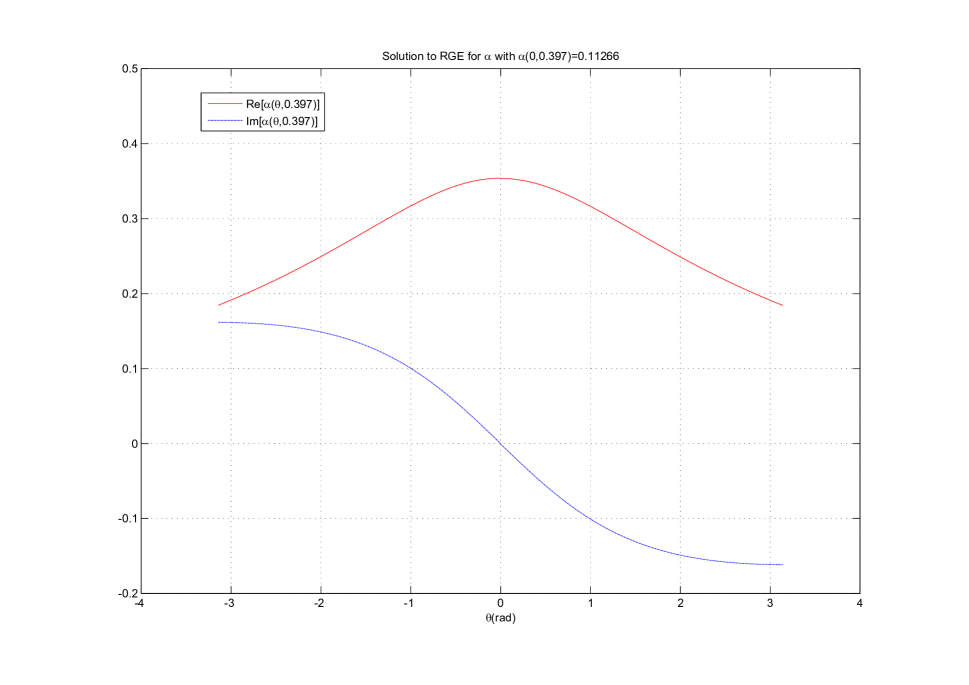
Figure 15: Numerical solution to the RGE for $\alpha_{s}(0,0.397)=0.11266$, with the top curve the real part and the bottom the imaginary part of $\alpha_{s}$

The above numerical solution matches that given in [40, 41]. From figure 15 we can see that the property given by (D.7) is valid. Now using (D.7) we can prove some interesting results about the integrals

$$f_{1} = \frac{{z_{0}\widetilde{m}^{2}\left({z_{0}}\right)}}{{2\pi i}}\int\limits_{-\pi}^{\pi}{\left({\pi+x}\right)a_{s}^{j}\left(x\right)\exp\left[{ix-2i\sum\limits_{l=0}^{3}{\gamma_{l}\int\limits_{0}^{x}{a_{s}^{l+1}\left({x^{\prime}}\right)}dx^{\prime}}}\right]dx}$$ (D.8)

$$f_{2} = \frac{{\left({-z_{0}}\right)^{n}\widetilde{m}^{2}\left({z_{0}}\right)}}{{2\pi}}\int\limits_{-\pi}^{\pi}{a_{s}^{j}\left(x\right)\exp\left[{inx-2i\sum\limits_{l=0}^{3}{\gamma_{l}\int\limits_{0}^{x}{a_{s}^{l+1}\left({x^{\prime}}\right)}dx^{\prime}}}\right]dx}\hfill$$ (D.9)

$$f_{3} = \frac{{\widetilde{m}^{2}\left({z_{0}}\right)}}{{2\pi}}\int\limits_{-\pi}^{\pi}{a_{s}^{j}\left(x\right)\exp\left[{-2i\sum\limits_{l=0}^{3}{\gamma_{l}\int\limits_{0}^{x}{a_{s}^{l+1}\left({x^{\prime}}\right)}dx^{\prime}}}\right]dx}$$ (D.10)

Consider the third integral

$$I_{j}^{\left(3\right)} = \int\limits_{-\pi}^{\pi}{a_{s}^{j}\left(x\right)\exp\left[{-2i\sum\limits_{l=0}^{3}{\gamma_{l}\int\limits_{0}^{x}{a_{s}^{l+1}\left(y\right)}dy}}\right]dx}$$ (D.11)

$$= \underline{\int\limits_{-\pi}^{0}{a_{s}^{j}\left(x\right)\exp\left[{-2i\sum\limits_{l=0}^{3}{\gamma_{l}\int\limits_{0}^{x}{a_{s}^{l+1}\left(y\right)}dy}}\right]dx}}+\int\limits_{0}^{\pi}{a_{s}^{j}\left(x\right)\exp\left[{-2i\sum\limits_{l=0}^{3}{\gamma_{l}\int\limits_{0}^{x}{a_{s}^{l+1}\left(y\right)}dy}}\right]dx}$$

for the underlined term we make a change of variables $x\mapsto x=-v$ $\Rightarrow$ $dx=-dv$ and we obtain

$$I_{j}^{\left(3\right)}=\int\limits_{0}^{\pi}{a_{s}^{j}\left({-v}\right)\exp\left[{-2i\sum\limits_{l=0}^{3}{\gamma_{l}\underline{\int\limits_{0}^{-v}{a_{s}^{l+1}\left(y\right)}dy}}}\right]dv}+\int\limits_{0}^{\pi}{a_{s}^{j}\left(x\right)\exp\left[{-2i\sum\limits_{l=0}^{3}{\gamma_{l}\int\limits_{0}^{x}{a_{s}^{l+1}\left(y\right)}dy}}\right]dx}$$ (D.12)

we make another change of variables with $y\mapsto y=-u$ $\Rightarrow$ $dy=-du$ and renaming $v$ as $x$ which leads to

$$I_{j}^{\left(3\right)} = \int\limits_{0}^{\pi}{a_{s}^{j}\left({-x}\right)\exp\left[{2i\sum\limits_{l=0}^{3}{\gamma_{l}\int\limits_{0}^{x}{a_{s}^{l+1}\left({-u}\right)}du}}\right]dx}+\int\limits_{0}^{\pi}{a_{s}^{j}\left(x\right)\exp\left[{-2i\sum\limits_{l=0}^{3}{\gamma_{l}\int\limits_{0}^{x}{a_{s}^{l+1}\left(y\right)}dy}}\right]dx}$$ (D.13)

$$= \int\limits_{0}^{\pi}{\overline{a}_{s}^{j}\left(x\right)\exp\left[{2i\sum\limits_{l=0}^{3}{\gamma_{l}\int\limits_{0}^{x}{\overline{a}_{s}^{l+1}\left(u\right)}du}}\right]dx}+\int\limits_{0}^{\pi}{a_{s}^{j}\left(x\right)\exp\left[{-2i\sum\limits_{l=0}^{3}{\gamma_{l}\int\limits_{0}^{x}{a_{s}^{l+1}\left(y\right)}dy}}\right]dx}$$

$$= \overline{\int\limits_{0}^{\pi}{a_{s}^{j}\left(x\right)\exp\left[{-2i\sum\limits_{l=0}^{3}{\gamma_{l}\int\limits_{0}^{x}{a_{s}^{l+1}\left(u\right)}du}}\right]dx}}+\int\limits_{0}^{\pi}{a_{s}^{j}\left(x\right)\exp\left[{-2i\sum\limits_{l=0}^{3}{\gamma_{l}\int\limits_{0}^{x}{a_{s}^{l+1}\left(y\right)}dy}}\right]dx}$$ (D.14)

$$= 2\operatorname{Re}\left\{{\int\limits_{0}^{\pi}{a_{s}^{j}\left(x\right)\exp\left[{-2i\sum\limits_{l=0}^{3}{\gamma_{l}\int\limits_{0}^{x}{a_{s}^{l+1}\left(y\right)}dy}}\right]dx}}\right\}$$ (D.15)

In (D.13) we have used the property of (D.7) and in (D.14) we taken out complex conjugate from the individual terms and conjugated the whole integral.

$${I_{j}^{\left(3\right)}=2\operatorname{Re}\left\{{\int\limits_{0}^{\pi}{a_{s}^{j}\left(x\right)\exp\left[{-2i\sum\limits_{l=0}^{3}{\gamma_{l}\int\limits_{0}^{x}{a_{s}^{l+1}\left(y\right)}dy}}\right]dx}}\right\}}$$ (D.16)

So the integral (D.16) is a purely real number.

We now consider the second integral

$$I_{j;n}^{\left(2\right)} = \int\limits_{-\pi}^{\pi}{a_{s}^{j}\left(x\right)\exp\left[{inx-2i\sum\limits_{l=0}^{3}{\gamma_{l}\int\limits_{0}^{x}{a_{s}^{l+1}\left(y\right)}dy}}\right]dx}$$ (D.17)

$$= \underline{\int\limits_{-\pi}^{0}{a_{s}^{j}\left(x\right)\exp\left[{inx-2i\sum\limits_{l=0}^{3}{\gamma_{l}\int\limits_{0}^{x}{a_{s}^{l+1}\left(y\right)}dy}}\right]dx}}+\int\limits_{0}^{\pi}{a_{s}^{j}\left(x\right)\exp\left[{inx-2i\sum\limits_{l=0}^{3}{\gamma_{l}\int\limits_{0}^{x}{a_{s}^{l+1}\left(y\right)}dy}}\right]dx}$$

we make a change of variables $x\mapsto x=-v$ $\Rightarrow$ $dx=-dv$ and we obtain

$$I_{j;n}^{\left(2\right)}=\int\limits_{0}^{\pi}{a_{s}^{j}\left({-v}\right)\exp\left[{-inv-2i\sum\limits_{l=0}^{3}{\gamma_{l}\underline{\int\limits_{0}^{-v}{a_{s}^{l+1}\left(y\right)}dy}}}\right]dv}+\int\limits_{0}^{\pi}{a_{s}^{j}\left(x\right)\exp\left[{inx-2i\sum\limits_{l=0}^{3}{\gamma_{l}\int\limits_{0}^{x}{a_{s}^{l+1}\left(y\right)}dy}}\right]dx}$$ (D.18)

we make another change of variables with $y\mapsto y=-u$ $\Rightarrow$ $dy=-du$ and renaming $v$ as $x$ which leads to

$$I_{j;n}^{\left(2\right)} =\int\limits_{0}^{\pi}{a_{s}^{j}\left({-x}\right)\exp\left[{-inx+2i\sum\limits_{l=0}^{3}{\gamma_{l}\int\limits_{0}^{x}{a_{s}^{l+1}\left({-u}\right)}du}}\right]dx}+\int\limits_{0}^{\pi}{a_{s}^{j}\left(x\right)\exp\left[{inx-2i\sum\limits_{l=0}^{3}{\gamma_{l}\int\limits_{0}^{x}{a_{s}^{l+1}\left(y\right)}dy}}\right]dx}$$

$$=\int\limits_{0}^{\pi}{\overline{a}_{s}^{j}\left(x\right)\exp\left[{-inx+2i\sum\limits_{l=0}^{3}{\gamma_{l}\int\limits_{0}^{x}{\overline{a}_{s}^{l+1}\left(u\right)}du}}\right]dx}+\int\limits_{0}^{\pi}{a_{s}^{j}\left(x\right)\exp\left[{inx-2i\sum\limits_{l=0}^{3}{\gamma_{l}\int\limits_{0}^{x}{a_{s}^{l+1}\left(y\right)}dy}}\right]dx}$$ (D.19)

$$=\overline{\int\limits_{0}^{\pi}{a_{s}^{j}\left(x\right)\exp\left[{inx-2i\sum\limits_{l=0}^{3}{\gamma_{l}\int\limits_{0}^{x}{a_{s}^{l+1}\left(u\right)}du}}\right]dx}}+\int\limits_{0}^{\pi}{a_{s}^{j}\left(x\right)\exp\left[{inx-2i\sum\limits_{l=0}^{3}{\gamma_{l}\int\limits_{0}^{x}{a_{s}^{l+1}\left(y\right)}dy}}\right]dx}$$ (D.20)

$$=2\operatorname{Re}\left\{{\int\limits_{0}^{\pi}{a_{s}^{j}\left(x\right)\exp\left[{inx-2i\sum\limits_{l=0}^{3}{\gamma_{l}\int\limits_{0}^{x}{a_{s}^{l+1}\left(y\right)}dy}}\right]dx}}\right\}$$ (D.21)

In (D.19) we have used the property of (D.7) and in (D.20) we have taken out the complex conjugate from the individual terms and conjugated the whole integral.

$${I_{j;n}^{\left(2\right)}=2\operatorname{Re}\left\{{\int\limits_{0}^{\pi}{a_{s}^{j}\left(x\right)\exp\left[{inx-2i\sum\limits_{l=0}^{3}{\gamma_{l}\int\limits_{0}^{x}{a_{s}^{l+1}\left(y\right)}dy}}\right]dx}}\right\}}$$ (D.22)

The integral (D.22) is again also a purely real number.

Now we finally consider the first integral. This is a problematic integral as it leads to a counter-intuitive conclusion.

$$I_{j}^{\left(1\right)} =\int\limits_{-\pi}^{\pi}{\left({\pi+x}\right)a_{s}^{j}\left(x\right)\exp\left[{ix-2i\sum\limits_{l=0}^{3}{\gamma_{l}\int\limits_{0}^{x}{a_{s}^{l+1}\left(y\right)}dy}}\right]dx}$$

$$=\underline{\int\limits_{-\pi}^{0}{\left({\pi+x}\right)a_{s}^{j}\left(x\right)\exp\left[{ix-2i\sum\limits_{l=0}^{3}{\gamma_{l}\int\limits_{0}^{x}{a_{s}^{l+1}\left(y\right)}dy}}\right]dx}}+$$

$$+\int\limits_{0}^{\pi}{\left({\pi+x}\right)a_{s}^{j}\left(x\right)\exp\left[{ix-2i\sum\limits_{l=0}^{3}{\gamma_{l}\int\limits_{0}^{x}{a_{s}^{l+1}\left(y\right)}dy}}\right]dx}$$ (D.23)

we make a change of variables $x\mapsto x=-v$ $\Rightarrow$ $dx=-dv$ and we obtain

$$I_{j}^{\left(1\right)}= \int\limits_{0}^{\pi}{\left({\pi-v}\right)a_{s}^{j}\left({-v}\right)\exp\left[{-iv-2i\sum\limits_{l=0}^{3}{\gamma_{l}\underline{\int\limits_{0}^{-v}{a_{s}^{l+1}\left(y\right)}dy}}}\right]dv}+$$

$$+\int\limits_{0}^{\pi}{\left({\pi+x}\right)a_{s}^{j}\left(x\right)\exp\left[{ix-2i\sum\limits_{l=0}^{3}{\gamma_{l}\int\limits_{0}^{x}{a_{s}^{l+1}\left(y\right)}dy}}\right]dx}$$ (D.24)

we make another change of variables with $y\mapsto y=-u$ $\Rightarrow$ $dy=-du$ and renaming $v$ as $x$ which leads to

$$I_{j}^{\left(1\right)}= \int\limits_{0}^{\pi}{\left({\pi-x}\right)a_{s}^{j}\left({-x}\right)\exp\left[{-ix+2i\sum\limits_{l=0}^{3}{\gamma_{l}\int\limits_{0}^{x}{a_{s}^{l+1}\left({-u}\right)}du}}\right]dx}+$$

$$+\int\limits_{0}^{\pi}{\left({\pi+x}\right)a_{s}^{j}\left(x\right)\exp\left[{ix-2i\sum\limits_{l=0}^{3}{\gamma_{l}\int\limits_{0}^{x}{a_{s}^{l+1}\left(y\right)}dy}}\right]dx}$$

$$= \int\limits_{0}^{\pi}{\left({\pi-x}\right)\overline{a}_{s}^{j}\left(x\right)\exp\left[{-ix+2i\sum\limits_{l=0}^{3}{\gamma_{l}\int\limits_{0}^{x}{\overline{a}_{s}^{l+1}\left(u\right)}du}}\right]dx}+$$

$$+\int\limits_{0}^{\pi}{\left({\pi+x}\right)a_{s}^{j}\left(x\right)\exp\left[{ix-2i\sum\limits_{l=0}^{3}{\gamma_{l}\int\limits_{0}^{x}{a_{s}^{l+1}\left(y\right)}dy}}\right]dx}$$ (D.25)

$$= \int\limits_{0}^{\pi}{\left({\pi-x}\right)\overline{a_{s}^{j}\left(x\right)\exp\left[{ix-2i\sum\limits_{l=0}^{3}{\gamma_{l}\int\limits_{0}^{x}{a_{s}^{l+1}\left(u\right)}du}}\right]}dx}+$$

$$+\int\limits_{0}^{\pi}{\left({\pi+x}\right)a_{s}^{j}\left(x\right)\exp\left[{ix-2i\sum\limits_{l=0}^{3}{\gamma_{l}\int\limits_{0}^{x}{a_{s}^{l+1}\left(y\right)}dy}}\right]dx}$$ (D.26)

$$= \pi\left[{\overline{\int\limits_{0}^{\pi}{a_{s}^{j}\left(x\right)\exp\left[{ix-2i\sum\limits_{l=0}^{3}{\gamma_{l}\int\limits_{0}^{x}{a_{s}^{l+1}\left(u\right)}du}}\right]dx}}+\int\limits_{0}^{\pi}{a_{s}^{j}\left(x\right)\exp\left[{ix-2i\sum\limits_{l=0}^{3}{\gamma_{l}\int\limits_{0}^{x}{a_{s}^{l+1}\left(u\right)}du}}\right]dx}}\right]$$

$$+\left[{\int\limits_{0}^{\pi}{xa_{s}^{j}\left(x\right)\exp\left[{ix-2i\sum\limits_{l=0}^{3}{\gamma_{l}\int\limits_{0}^{x}{a_{s}^{l+1}\left(y\right)}dy}}\right]dx}-\overline{\int\limits_{0}^{\pi}{xa_{s}^{j}\left(x\right)\exp\left[{ix-2i\sum\limits_{l=0}^{3}{\gamma_{l}\int\limits_{0}^{x}{a_{s}^{l+1}\left(y\right)}dy}}\right]dx}}}\right]$$ (D.27)

$$= 2\pi\operatorname{Re}\left\{{\int\limits_{0}^{\pi}{a_{s}^{j}\left(x\right)\exp\left[{ix-2i\sum\limits_{l=0}^{3}{\gamma_{l}\int\limits_{0}^{x}{a_{s}^{l+1}\left(u\right)}du}}\right]dx}}\right\}+$$

$$+2i\operatorname{Im}\left\{{\int\limits_{0}^{\pi}{xa_{s}^{j}\left(x\right)\exp\left[{ix-2i\sum\limits_{l=0}^{3}{\gamma_{l}\int\limits_{0}^{x}{a_{s}^{l+1}\left(y\right)}dy}}\right]dx}}\right\}$$

$$= \pi I_{j;1}^{\left(2\right)}+2i\operatorname{Im}\left\{{\int\limits_{0}^{\pi}{xa_{s}^{j}\left(x\right)\exp\left[{ix-2i\sum\limits_{l=0}^{3}{\gamma_{l}\int\limits_{0}^{x}{a_{s}^{l+1}\left(y\right)}dy}}\right]dx}}\right\}$$ (D.29)

In (D.25) we have used the property of (D.7) and in (D.26) we have taken out the complex conjugate from the individual terms and conjugated the whole integral. In (D.27) we have gathered the integrals and their complex conjugates and in (D.29), we noted that the first term of (LABEL:link0) is just the case of (D.22) with $n=1$.

$${I_{j}^{\left(1\right)}=\pi I_{j;1}^{\left(2\right)}+2i\operatorname{Im}\left\{{\int\limits_{0}^{\pi}{xa_{s}^{j}\left(x\right)\exp\left[{ix-2i\sum\limits_{l=0}^{3}{\gamma_{l}\int\limits_{0}^{x}{a_{s}^{l+1}\left(y\right)}dy}}\right]dx}}\right\}}$$ (D.30)

The integral (D.30) is a part real and part imaginary number! This is problematic as the integral (D.8) has an additional factor of $1/i$ on the outside of the integral. From the result of (D.30) we can conclude that the result of the calculation for $\delta_{5}$ will have an imaginary component to it. This is bad as the quantity we are trying to calculate is a purely real number!

Appendix E Coefficient fixing of $\Delta(z)$

The purpose of introducing a kernel (B.2) in the calculation of the $\delta_{5}(R)$ was to minimise the effect of the resonance terms. This is done by insisting that $\Delta(M^{2}_{1})=0$ and $\Delta(M^{2}_{2})=0$ where $M^{2}_{1}$ and $M^{2}_{2}$ are the squared masses of the resonances of the Kaon particle

$$\Delta\left({{\rm M}_{1}^{2}}\right)=1-a_{0}{\rm M}_{1}^{2}-a_{1}{\rm M}_{1}^{4}=0$$ (E.1)

$$\Delta\left({{\rm M}_{2}^{2}}\right)=1-a_{0}{\rm M}_{2}^{2}-a_{1}{\rm M}_{2}^{4}=0$$ (E.2)

solving the above equations simultaneously leads to

$$a_{0} = \frac{{{\rm M}_{\rm 1}^{\rm 2}+{\rm M}_{\rm 2}^{\rm 2}}}{{{\rm M}_{\rm 1}^{\rm 2}{\rm M}_{\rm 2}^{\rm 2}}}$$ (E.3)

$$a_{1} = -\frac{1}{{{\rm M}_{\rm 1}^{\rm 2}{\rm M}_{\rm 2}^{\rm 2}}}$$ (E.4)

The masses are excited states of the Kaon [33] which are $M_{1}=1.40$ GeV and $M_{2}=1.94$ GeV. This leads to

$$a_{0} = 0.7759/\rm{GeV^{2}}$$

$$a_{1} = -0.1355/\rm{GeV^{4}}$$

For the Pion the excited states have masses which are $M_{1}=1.30$ GeV and $M_{2}=1.81$ GeV. This leads to

$$a_{0} = 0.8949/\rm{GeV^{2}}$$

$$a_{1} = -0.1794/\rm{GeV^{4}}$$

Appendix F Perturbative QCD Integrals

General integrals of the form ${\rm I}_{{\rm nk}}$ are required to do the calculations with

$${\rm I}_{{\rm nk}}=\frac{1}{{2\pi i}}\oint\limits_{C^{\prime}(r)}{z^{n}\left[{\ln\left({-z}\right)}\right]^{k}dz}$$

where $C^{\prime}(r)$ is the contour chosen to be a circle of radius $r$ parameterized from $-\pi$ to $\pi$ and $n,k$ $\in\mathbb{N}$.

For $n\geq 0$ and $k\geq 0$

$$\sigma_{jn}=\left\{{\begin{array}[]{*{20}lcr}{\left({-1}\right)^{j+1}{\rm;n}\in{\rm 2\mathbb{N}}}\\ {\left({-1}\right)^{j}{\hskip 9.95863pt\rm;n}\in{\rm 2\mathbb{N}+1}}\\ \end{array}}\right.$$

$$\beta_{knj}=\frac{{k!\left({n+1}\right)^{k-j}}}{{\left({k-j}\right)!}}$$

$$a=\rm ln\emph{r}$$

$${\rm I}_{{\rm nk}}=\frac{{\left({-r}\right)^{n+1}}}{{2\pi i\left({n+1}\right)^{k+1}}}\sum\limits_{j=0}^{k}{\beta_{knj}\sigma_{jn}\left[{\left({a+i\pi}\right)^{k-j}-\left({a-i\pi}\right)^{k-j}}\right]}$$ (F.1)

Using (F.1) we computed the following integrals

$${\rm I}_{01} = r$$ (F.2)

$${\rm I}_{11} = \frac{1}{2}r^{2}$$ (F.3)

$${\rm I}_{21} = \frac{1}{3}r^{3}$$ (F.4)

$${\rm I}_{02} = 2r\left[{\ln r-1}\right]$$ (F.5)

$${\rm I}_{12} = r^{2}\left[{\ln r-\frac{1}{2}}\right]$$ (F.6)

$${\rm I}_{22} = \frac{2}{9}r^{3}\left[{3\ln r-1}\right]$$ (F.7)

$${\rm I}_{03} = r\left[{3\left({\ln^{2}r-2\ln r}\right)+6-\pi^{2}}\right]$$ (F.8)

$${\rm I}_{13} = r^{2}\left[{\frac{3}{2}\left({\ln^{2}r-\ln r}\right)+\frac{3}{4}-\frac{1}{2}\pi^{2}}\right]$$ (F.9)

$${\rm I}_{23} = r^{3}\left[{\left({\ln^{3}r-2\ln r}\right)+\frac{2}{9}-\frac{1}{3}\pi^{2}}\right]$$ (F.10)

$${\rm I}_{{\rm 04}} = r\left[{4\ln^{3}r-12\ln^{2}r+4\left({6-\pi^{2}}\right)\ln r+4\left({\pi^{2}-6}\right)}\right]$$ (F.11)

$${\rm I}_{{\rm 14}} = r^{2}\left[{2\ln^{3}r-3\ln^{2}r+\left({3-2\pi^{2}}\right)\ln r+\pi^{2}-\frac{3}{2}}\right]$$ (F.12)

$${\rm I}_{{\rm 24}} = r^{3}\left[{\frac{4}{3}\left({\ln^{3}r-\ln^{2}r+\left({\frac{2}{3}-\pi^{2}}\right)\ln r}\right)+\frac{4}{3}\left({\pi^{2}-\frac{2}{3}}\right)}\right]$$ (F.13)

$${\rm I}_{{\rm 05}} = r\left[{5\ln^{4}r-20\ln^{3}r+10\left({\ln r-2}\right)\left({6-\pi^{2}}\right)\ln r+\pi^{4}-20\pi^{2}+120}\right]$$ (F.14)

$${\rm I}_{{\rm 15}} = r^{2}\left[{\frac{5}{2}\ln^{4}r-5\ln^{3}r+5\left({\ln r-1}\right)\left({\frac{3}{2}-\pi^{2}}\right)\ln r+\frac{{\pi^{4}}}{2}-\frac{5}{2}\pi^{2}+\frac{{15}}{4}}\right]$$ (F.15)

$${\rm I}_{{\rm 25}} = r^{3}\left[{\frac{5}{3}\ln^{4}r-\frac{{20}}{9}\ln^{3}r+\frac{{10}}{3}\left({\ln r-\frac{2}{3}}\right)\left({\frac{6}{9}-\pi^{2}}\right)\ln r+\frac{{\pi^{4}}}{3}-\frac{{20}}{{27}}\pi^{2}+\frac{{40}}{{81}}}\right]$$ (F.16)

Appendix G The Resonance Integrals

To compute the resonance contribution, $\left.{\delta_{5}\left(R\right)}\right|_{RES}$, to the FESR we need to compute integrals of the form

$$\int\limits_{9M_{\pi}^{2}}^{R}{\frac{1}{z}\Delta\left(z\right)z\Theta\left(z\right)BW_{k}\left(z\right)dz}$$ (G.1)

with the Breit-Wigner profile

$$BW_{k}\left(z\right)=\frac{{M_{k}^{2}\left({M_{k}^{2}+\Gamma_{k}^{2}}\right)}}{{\left({z-M_{k}^{2}}\right)^{2}+M_{k}^{2}\Gamma_{k}^{2}}}$$ (G.2)

defining for convenience the following

$$\begin{gathered}\alpha^{2}\equiv M_{k}^{2}\left({M_{k}^{2}+\Gamma_{k}^{2}}\right)\hfill\\ \beta^{2}\equiv M_{k}^{2}\hfill\\ \gamma^{2}\equiv M_{k}^{2}\Gamma_{k}^{2}\hfill\\ \end{gathered}$$

Now substituting (G.2) into (G.1)

$$\int{\Delta\left(z\right)\frac{{\alpha^{2}}}{{\left({z-\beta^{2}}\right)^{2}+\gamma^{2}}}dz}=\alpha^{2}\left\{{\int{\frac{1}{{\left({z-\beta^{2}}\right)^{2}+\gamma^{2}}}dz}-a_{0}\int{\frac{z}{{\left({z-\beta^{2}}\right)^{2}+\gamma^{2}}}dz}-a_{1}\int{\frac{{z^{2}}}{{\left({z-\beta^{2}}\right)^{2}+\gamma^{2}}}dz}}\right\}$$ (G.3)

the first integral can be easily integrated as

$$\int{\frac{1}{{\left({z-\beta^{2}}\right)^{2}+\gamma^{2}}}dz} = \frac{1}{{\gamma^{2}}}\int{\frac{1}{{\left({\frac{{z-\beta^{2}}}{\gamma}}\right)^{2}+1}}dz}$$ (G.4)

$$= \frac{1}{\gamma}\arctan\left({\frac{{z-\beta^{2}}}{\gamma}}\right)$$

the second and third integrals require some work

$$\int{\frac{z}{{\left({z-\beta^{2}}\right)^{2}+\gamma^{2}}}dz} = \int{\frac{{z-\beta^{2}+\beta^{2}}}{{\left({z-\beta^{2}}\right)^{2}+\gamma^{2}}}dz}$$ (G.5)

$$= \int{\frac{{z-\beta^{2}}}{{\left({z-\beta^{2}}\right)^{2}+\gamma^{2}}}dz}+\int{\frac{{\beta^{2}}}{{\left({z-\beta^{2}}\right)^{2}+\gamma^{2}}}dz}$$

$$= \frac{1}{2}\ln\left[{\left({z-\beta^{2}}\right)^{2}+\gamma^{2}}\right]+\frac{{\beta^{2}}}{\gamma}\arctan\left({\frac{{z-\beta^{2}}}{\gamma}}\right)$$

For the third integral we make use of a substitution $u=z-\beta^{2}$ $\Rightarrow$ $dz=du$ so

$$\int{\frac{{z^{2}}}{{\left({z-\beta^{2}}\right)^{2}+\gamma^{2}}}dz} = \int{\frac{{u^{2}+2u\beta^{2}+\beta^{4}}}{{u^{2}+\gamma^{2}}}du}$$ (G.6)

$$= \int{\frac{{u^{2}}}{{u^{2}+\gamma^{2}}}du}+2\beta^{2}\int{\frac{u}{{u^{2}+\gamma^{2}}}du}+\beta^{4}\int{\frac{1}{{u^{2}+\gamma^{2}}}du}$$

$$= \int{\frac{{u^{2}+\gamma^{2}-\gamma^{2}}}{{u^{2}+\gamma^{2}}}du}+2\beta^{2}\int{\frac{u}{{u^{2}+\gamma^{2}}}du}+\beta^{4}\int{\frac{1}{{u^{2}+\gamma^{2}}}du}$$

$$= u+\left({\beta^{4}-\gamma^{2}}\right)\int{\frac{1}{{u^{2}+\gamma^{2}}}du}+2\beta^{2}\int{\frac{u}{{u^{2}+\gamma^{2}}}du}$$

$$= u+\left({\frac{{\beta^{4}-\gamma^{2}}}{{\gamma^{2}}}}\right)\int{\frac{1}{{\left({\frac{u}{\gamma}}\right)^{2}+1}}du}+2\beta^{2}\int{\frac{u}{{u^{2}+\gamma^{2}}}du}$$

$$= u+\left({\frac{{\beta^{4}-\gamma^{2}}}{\gamma}}\right)\arctan\left({\frac{u}{\gamma}}\right)+\beta^{2}\ln\left({u^{2}+\gamma^{2}}\right)$$

$$= z-\beta^{2}+\left({\frac{{\beta^{4}-\gamma^{2}}}{\gamma}}\right)\arctan\left({\frac{{z-\beta^{2}}}{\gamma}}\right)+\beta^{2}\ln\left[{\left({z-\beta^{2}}\right)^{2}+\gamma^{2}}\right]$$

now substituting the integrals (G.4 - G.6) into the right-hand side of (G.3)

$$\alpha^{2}\left\{{\int{\frac{1}{{\left({z-\beta^{2}}\right)^{2}+\gamma^{2}}}dz}-a_{0}\int{\frac{z}{{\left({z-\beta^{2}}\right)^{2}+\gamma^{2}}}dz}-a_{1}\int{\frac{{z^{2}}}{{\left({z-\beta^{2}}\right)^{2}+\gamma^{2}}}dz}}\right\}$$

$$= \alpha^{2}\left\{{\frac{1}{\gamma}\left[{1-a_{0}\beta^{2}-a_{1}\left({\beta^{4}-\gamma^{2}}\right)}\right]\arctan\left({\frac{{z-\beta^{2}}}{\gamma}}\right)-\left({\frac{1}{2}a_{0}+a_{1}\beta^{2}}\right)\ln\left[{\left({z-\beta^{2}}\right)^{2}+\gamma^{2}}\right]-a_{1}\left({z-\beta^{2}}\right)}\right\}$$ (G.7)

getting rid of the $\alpha,\beta$ and $\gamma$ by substituting in their definitions into (G.7) and now defining a new function $G_{k}\left(z\right)$ as the right-hand side of (G.7) we get

$$\!\!\!\!G_{k}\left(z\right)=M_{k}^{2}\left({M_{k}^{2}+\Gamma_{k}^{2}}\right) \Biggl{\{}\frac{1}{{M_{k}\Gamma_{k}}}\left[{1-a_{0}M_{k}^{2}-a_{1}\left({M_{k}^{4}-M_{k}^{2}\Gamma_{k}^{2}}\right)}\right]\arctan\left({\frac{{z-M_{k}^{2}}}{{M_{k}\Gamma_{k}}}}\right)+$$

$$-\left({\frac{1}{2}a_{0}+a_{1}M_{k}^{2}}\right)\ln\left[{\left({z-M_{k}^{2}}\right)^{2}+M_{k}^{2}\Gamma_{k}^{2}}\right]-a_{1}\left({z-M_{k}^{2}}\right)\Biggr{\}}$$

we have ignored the constant of integration in (LABEL:resintfinal) since (G.1) is a definite integral and when we evaluate using (LABEL:resintfinal), what ever constant that was there would subtract to zero.

Finally leading to

$$\int\limits_{9M_{\pi}^{2}}^{R}{\frac{1}{z}\Delta\left(z\right)z\Theta\left(z\right)BW_{k}\left(z\right)dz}=G_{k}\left(R\right)-G_{k}\left({9M_{\pi}^{2}}\right)$$ (G.9)

Appendix H Exact solution of the RGE for $\alpha_{s}$ up to fifth order

A problem that has been on the authors mind is that of an exact solution to the Renormalization Group Equation(RGE) . Finding exact solutions has turned into a slight obsession! So on a lighter note we attempt to produce an exact solution to the RGE for the strong coupling $\alpha_{s}$

The evolution of $\alpha_{s}$ is governed by the differential equation

$$\frac{{d{\rm a}_{\rm s}(x)}}{{dx}}=-i\sum\limits_{n=0}^{3}{\beta_{n}{\rm a}_{\rm s}^{{\rm n+2}}(x)}$$ (H.1)

which is expanded into

$$\frac{{d{a_{s}}(x)}}{dx}=-i\left[\beta_{0}a_{s}^{2}+\beta_{1}a_{s}^{3}+\beta_{2}a_{s}^{4}+\beta_{3}a_{s}^{5}\right]$$ (H.2)

factoring out $\beta_{3}a_{s}^{2}$ we obtain

$$\frac{{d{a_{s}}(x)}}{dx}=-i\beta_{3}a_{s}^{2}\left[a_{s}^{3}+\frac{\beta_{2}}{\beta_{3}}a_{s}^{2}+\frac{\beta_{1}}{\beta_{3}}a_{s}+\frac{\beta_{0}}{\beta_{3}}\right]$$ (H.3)

for convenience we rename $a_{s}\rightarrow z$ and let

$$\begin{array}[]{l}a=\frac{\beta_{2}}{\beta_{3}}\\ \\ b=\frac{\beta_{1}}{\beta_{3}}\\ \\ c=\frac{\beta_{0}}{\beta_{3}}\\ \end{array}$$ (H.9)

we then obtain

$$\frac{{dz(x)}}{{dx}}=-i\beta_{3}z^{2}\left[{z^{3}+az^{2}+bz+c}\right]$$ (H.10)

So this is the differential equation that must be solved to find the evolution of the strong coupling $z$ we note at this point that there is a cubic polynomial on the right-hand side of the above equation

$$p\left(z\right)=z^{3}+az^{2}+bz+c$$ (H.11)

for

$$\mathop{\lim}\limits_{z\to+\infty}p\left(z\right)\to+\infty$$ (H.12)

$$\mathop{\lim}\limits_{z\to-\infty}p\left(z\right)\to-\infty$$ (H.13)

now by the Intermediate Value Theorem/Bolzano’s Theorem [42] we are guaranteed of the existence of at least one root of $p(z)$. Let $z=\alpha$ be this root so $p(\alpha)=0$, then we can proceed with long division on $p(z)$ and write $p(z)$ as a product of lower order polynomials i.e.

$$p\left(z\right)=\left({z-\alpha}\right)\left[{z^{2}+ez+f}\right]$$

with

$$\begin{array}[]{l}e=a+\alpha\\ f=b+\alpha a+\alpha^{2}\\ \end{array}$$

So getting back to the problem of the solution to the differential equation we can now write (H.10) as

$$\frac{{dz(x)}}{{dx}}=-i\beta_{3}z^{2}\left({z-\alpha}\right)\left[{z^{2}+ez+f}\right]$$

This is a separable differential equation so

$$\int{-i\beta_{3}\textit{ }dx}=\int{\frac{{dz}}{{z^{2}\left({z-\alpha}\right)\left[{z^{2}+ez+f}\right]}}}$$ (H.14)

The left hand side is trivially integrated but the right-hand side requires some work, we note that the integrand can be expressed as

$$\frac{1}{{z^{2}\left({z-\alpha}\right)\left[{z^{2}+ez+f}\right]}}=\frac{{Az+D}}{{z^{2}}}+\frac{B}{{\left({z-\alpha}\right)}}+\frac{{Cz+E}}{{\left[{z^{2}+ez+f}\right]}}$$

with a suitable choice of the coefficients $A,B,C,D,E$ we shall expand more about how they are chosen, by simplifying the above expression and using a common denominator we have:

$$\frac{1}{{z^{2}\left({z-\alpha}\right)\left[{z^{2}+ez+f}\right]}}$$

$$= \frac{{(A+B+C)z^{4}+\left[{(e-\alpha)A+eB-\alpha C+D+E}\right]z^{3}+\left[{(f-e\alpha)A+fB+(e-\alpha)D-\alpha E}\right]z^{2}}}{{z^{2}\left({z-\alpha}\right)\left[{z^{2}+ez+f}\right]}}$$

$$+ \frac{{\left[{-\alpha fA+(f-e\alpha)D}\right]z-\alpha fD}}{{z^{2}\left({z-\alpha}\right)\left[{z^{2}+ez+f}\right]}}$$ (H.15)

since the numerator of left-hand side of (H.15) is a polynomial of order zero the numerator of the right-hand side also has to be a polynomial of order zero so we have to have

$$A+B+C = 0$$ (H.16)

$$(e-\alpha)A+eB-\alpha C+D+E = 0$$

$$(f-e\alpha)A+fB+(e-\alpha)D-\alpha E = 0$$

$$-\alpha fA+(f-e\alpha)D = 0$$

$$-\alpha fD = 1$$

we now have a system of five equations with five unknowns which can be solved uniquely to give

$$A = -\frac{{f-e\alpha}}{{\alpha^{2}f^{2}}}$$ (H.17)

$$B = \frac{1}{{\alpha^{2}\left({\alpha^{2}+e\alpha+f}\right)}}$$ (H.18)

$$C = \frac{{f-e^{2}-e\alpha}}{{f^{2}\left({\alpha^{2}+e\alpha+f}\right)}}$$ (H.19)

$$D = -\frac{1}{{\alpha f}}$$ (H.20)

$$E = \frac{{\left({f-e^{2}}\right)\alpha+\left({2f-e^{2}}\right)e}}{{f^{2}\left({\alpha^{2}+e\alpha+f}\right)}}$$ (H.21)

so the integral

$$\int{\frac{{dz}}{{z^{2}\left({z-\alpha}\right)\left[{z^{2}+ez+f}\right]}}}$$

can be expressed as

$$\int{\left[{\frac{{Az+D}}{{z^{2}}}+\frac{B}{{\left({z-\alpha}\right)}}+\frac{{Cz+E}}{{\left[{z^{2}+ez+f}\right]}}}\right]dz}$$

and then simplifying a bit

$$\int{\left[{\frac{A}{z}+\frac{D}{{z^{2}}}+\frac{B}{{\left({z-\alpha}\right)}}+\frac{C}{2}\frac{{2z+e-e}}{{\left[{z^{2}+ez+f}\right]}}+\frac{E}{{\left[{z^{2}+ez+f}\right]}}}\right]dz}$$

then separating the fourth term and combining with the fifth

$$\int{\left[{\frac{A}{z}+\frac{D}{{z^{2}}}+\frac{B}{{\left({z-\alpha}\right)}}+\frac{C}{2}\frac{{2z+e}}{{\left[{z^{2}+ez+f}\right]}}+\left[{E-\frac{1}{2}eC}\right]\frac{1}{{\left[{z^{2}+ez+f}\right]}}}\right]dz}$$

now completing the square on the denominator of the last term we obtain

$$\int{\left[{\frac{A}{z}+\frac{D}{{z^{2}}}+\frac{B}{{\left({z-\alpha}\right)}}+\frac{C}{2}\frac{{2z+e}}{{\left[{z^{2}+ez+f}\right]}}+\left[{E-\frac{1}{2}eC}\right]\frac{1}{{\left[{\left({z+\frac{1}{2}e}\right)^{2}+\frac{{4f-e^{2}}}{4}}\right]}}}\right]dz}$$

if

$${\frac{{4f-e^{2}}}{4}}>0$$

then

$$\int{\left[{\frac{A}{z}+\frac{D}{{z^{2}}}+\frac{B}{{\left({z-\alpha}\right)}}+\frac{C}{2}\frac{{2z+e}}{{\left[{z^{2}+ez+f}\right]}}+\left[{E-\frac{1}{2}eC}\right]\frac{4}{{4f-e^{2}}}\frac{1}{{\left[{\frac{4}{{4f-e^{2}}}\left({z+\frac{1}{2}e}\right)^{2}+1}\right]}}}\right]dz}$$ (H.22)

we can now integrate (H.22) exactly to give

$$A\ln z-\frac{D}{z}+B\ln\left({z-\alpha}\right)+\frac{1}{2}C\ln\left({z^{2}+ez+f}\right)+\frac{{2\left({E-\frac{1}{2}eC}\right)}}{{\sqrt{4f-e^{2}}}}\arctan\left[{\frac{{2\left({z+\frac{1}{2}e}\right)}}{{\sqrt{4f-e^{2}}}}}\right]+G$$

where G is the constant of integration, we can tidy the above equation by combining the logarithmic terms together to give

$$\ln\left[{z^{A}\left({z-\alpha}\right)^{B}\left({z^{2}+ez+f}\right)^{C/2}}\right]-\frac{D}{z}+\frac{{2\left({E-\frac{1}{2}eC}\right)}}{{\sqrt{4f-e^{2}}}}\arctan\left[{\frac{{2\left({z+\frac{1}{2}e}\right)}}{{\sqrt{4f-e^{2}}}}}\right]+G$$ (H.23)

now (H.23) is the right-hand side of (H.14) which gives

$$-i\beta_{3}x=\ln\left[{z^{A}\left({z-\alpha}\right)^{B}\left({z^{2}+ez+f}\right)^{{C/2}}}\right]-\frac{D}{z}+\frac{{2\left({E-\frac{1}{2}eC}\right)}}{{\sqrt{4f-e^{2}}}}\arctan\left[{\frac{{2\left({z+\frac{1}{2}e}\right)}}{{\sqrt{4f-e^{2}}}}}\right]+G$$ (H.24)

and now changing back to the original notation

$$-i\beta_{3}x=\ln\left[a_{s}^{A}\left(a_{s}-\alpha\right)^{B}\left({a_{s}^{2}+ea_{s}+f}\right)^{C/2}\right]-\frac{D}{{a_{s}}}+\frac{{2\left({E-\frac{1}{2}eC}\right)}}{{\sqrt{4f-e^{2}}}}\arctan\left[{\frac{{2\left({a_{s}+\frac{1}{2}e}\right)}}{{\sqrt{4f-e^{2}}}}}\right]+G$$ (H.25)

Now equation (H.1) was obtained from the following change of variables $y=y_{0}e^{ix}$ now reverting back to the original notation for $a_{s}(y)$ we obtain

$$-\beta_{3}\ln\left(\frac{y}{y_{0}}\right)=\ln\left[a_{s}^{A}\left(a_{s}-\alpha\right)^{B}\left({a_{s}^{2}+ea_{s}+f}\right)^{C/2}\right]-\frac{D}{{a_{s}}}+\frac{{2\left({E-\frac{1}{2}eC}\right)}}{{\sqrt{4f-e^{2}}}}\arctan\left[{\frac{{2\left({a_{s}+\frac{1}{2}e}\right)}}{{\sqrt{4f-e^{2}}}}}\right]+G$$ (H.26)

This is an exact solution to the RGE for $a_{s}(y)$ up to fifth order $a_{s}(y)$!

We have tried with very little success to invert (H.26) to get $a_{s}(y)$ but we have had no success. To check intuitively if this gives the right behavior we expect that for large $y$ which corresponds to large energies, the coupling will tend to zero so

$$\mathop{\lim}\limits_{y\to\infty}{\rm LHS} =\mathop{\lim}\limits_{y\to\infty}\left[{-\beta_{3}\ln\left(\frac{y}{y_{0}}\right)}\right]\to-\infty$$

$$\mathop{\lim}\limits_{a_{s}\to 0^{+}}{\rm RHS} =\mathop{\lim}\limits_{a_{s}\to 0^{+}}\Biggl{[}A\ln a_{s}-\frac{D}{{a_{s}}}+B\ln\left({a_{s}-\alpha}\right)+\frac{1}{2}C\ln\left({a_{s}^{2}+ea_{s}+f}\right)+$$

$$+\frac{{2\left({E-\frac{1}{2}eC}\right)}}{{\sqrt{4f-e^{2}}}}\arctan\left[{\frac{{2\left({a_{s}+\frac{1}{2}e}\right)}}{{\sqrt{4f-e^{2}}}}}\right]+G\Biggr{]}$$

$$=\mathop{\lim}\limits_{a_{s}\to 0^{+}}\left[{A\ln a_{s}-\frac{D}{{a_{s}}}}\right]\to-\infty$$

so the limits of left and right-hand side agrees and behaves according to our intuition for the high energies/small coupling. On the other hand we expect that for small energies the coupling tends to large values,

$$\mathop{\lim}\limits_{y\to y_{0}^{+}}{\rm LHS} =\mathop{\lim}\limits_{y\to y_{0}^{+}}\left[{-\beta_{3}\ln\left(\frac{y}{y_{0}}\right)}\right]\to 0$$

$$\mathop{\lim}\limits_{a_{s}\to\infty}{\rm RHS} =\mathop{\lim}\limits_{a_{s}\to\infty}\left[{\ln\left[{a_{s}}^{A}\left({a_{s}-\alpha}\right)^{B}\left({a_{s}^{2}+ea_{s}+f}\right)^{C/2}\right]-\frac{D}{{a_{s}}}+\frac{{2\left({E-\frac{1}{2}eC}\right)}}{{\sqrt{4f-e^{2}}}}\arctan\left[{\frac{{2\left({a_{s}+\frac{1}{2}e}\right)}}{{\sqrt{4f-e^{2}}}}}\right]+G}\right]$$

$$=\mathop{\lim}\limits_{a_{s}\to\infty}\ln\left[a_{s}^{A}\left({a_{s}-\alpha}\right)^{B}\left({a_{s}^{2}+ea_{s}+f}\right)^{C/2}\right]$$

$$=\mathop{\lim}\limits_{a_{s}\to\infty}\ln\left[a_{s}^{A}a_{s}^{B}\left({1-\frac{\alpha}{{a_{s}}}}\right)^{B}a_{s}^{C}\left({1+\frac{e}{{a_{s}}}+\frac{f}{{a_{s}^{2}}}}\right)^{C/2}\right]$$

$$=\mathop{\lim}\limits_{a_{s}\to\infty}\ln\left[a_{s}^{A+B+C}\left({1-\frac{\alpha}{{a_{s}}}}\right)^{B}\left({1+\frac{e}{{a_{s}}}+\frac{f}{{a_{s}^{2}}}}\right)^{{C/2}}\right]$$

but from (H.16): $A+B+C=0$ we see that

$$\mathop{\lim}\limits_{a_{s}\to\infty}{\rm RHS} = \mathop{\lim}\limits_{a_{s}\to\infty}\ln\left[\left({1-\frac{\alpha}{{a_{s}}}}\right)^{B}\left({1+\frac{e}{a_{s}}+\frac{f}{a_{s}^{2}}}\right)^{C/2}\right]$$

$$\mathop{\lim}\limits_{a_{s}\to\infty}{\rm RHS} = \mathop{\lim}\limits_{a_{s}\to\infty}\ln\left[\left({1-0}\right)^{B}\left({1+0+0}\right)^{C/2}\right]\to 0$$

so the limits of left and right-hand side agrees and behaves according to our intuition for the small energies/high coupling! We have to be careful when taking the limit of the LHS as $y\rightarrow 0^{+}$ as the LHS tends to $+\infty$. This is just the result of the truncation of the series expansion of the QCD $\beta(a_{s})$ function and if we had managed to include all the terms, this divergence would not show up!

This (H.25) is the general class of solutions, to fix $G$ we need $y,a_{s}(y)$ at a particular point.

This exact solution rests upon the fact that we can find the root $\alpha$ such that $p(\alpha)=0$, but how is this done? The method to find the root of the cubic was developed by the mathematician Cardano to provide an exact solution to the roots of a cubic function.

References

- [1] David H Politzer. Reliable perturbative results for strong interactions? Physical Review Letters, 30(26):1346, 1973.
- [2] David J Gross and Frank Wilczek. Ultraviolet behavior of non-abelian gauge theories. Physical Review Letters, 30(26):1343, 1973.
- [3] Mikhail A Shifman, Arkady I Vainshtein, and Valentin I Zakharov. QCD and resonance physics. theoretical foundations. Nuclear Physics B, 147(5):385–447, 1979.
- [4] Mikhail A Shifman, AI Vainshtein, and Valentin I Zakharov. QCD and resonance physics. applications. Nuclear Physics B, 147(5):448–518, 1979.
- [5] Matthias Jamin. Flavour-symmetry breaking of the quark condensate and chiral corrections to the Gell-Mann–Oakes–Renner relation. Physics Letters B, 538(1-2):71–76, 2002.
- [6] CA Dominguez, A Ramlakan, and K Schilcher. Ratio of strange to non-strange quark condensates in QCD. Physics Letters B, 511(1):59–65, 2001.
- [7] William I Weisberger. Renormalization of the weak axial-vector coupling constant. Physical Review Letters, 14(25):1047, 1965.
- [8] Stephen L Adler. Consistency conditions on the strong interactions implied by a partially conserved axial-vector current. Physical Review, 137(4B):B1022, 1965.
- [9] Stephen L Adler. Sum rules for the axial-vector coupling-constant renormalization in decay. Physical Review, 140(3B):B736, 1965.
- [10] Ian D Lawrie. A unified grand tour of theoretical physics. Taylor & Francis, 2012.
- [11] Lewis H Ryder. Quantum field theory. Cambridge university press, 1996.
- [12] Pietro Colangelo and Alexander Khodjamirian. QCD sum rules, a modern perspective. In At The Frontier of Particle Physics: Handbook of QCD (in 3 Volumes), pages 1495–1576. World Scientific, 2001.
- [13] Elias M Stein and Rami Shakarchi. Real analysis, Princeton Lectures in Analysis III, 2005.
- [14] George B Arfken, Hans J Weber, and Frank E Harris. Mathematical methods for physicists: a comprehensive guide. Academic press, 2011.
- [15] Louis Legendre Pennisi, Louis I Gordon, and Sim Lasher. Elements of complex variables. 1963.
- [16] Fernando Bodí-Esteban, J Bordes, and J Penarrocha. B and b s decay constants from moments of finite energy sum rules in QCD. The European Physical Journal C-Particles and Fields, 38:277–281, 2004.
- [17] J Penarrocha and K Schilcher. QCD duality and the mass of the charm quark. Physics Letters B, 515(3-4):291–296, 2001.
- [18] Martin Beneke and Matthias Jamin. and the hadronic width: fixed-order, contour-improved and higher-order perturbation theory. Journal of High Energy Physics, 2008(09):044, 2008.
- [19] Cesareo A Dominguez, Nasrallah F Nasrallah, and Karl Schilcher. Strange quark condensate from QCD sum rules to five loops. Journal of High Energy Physics, 2008(02):072, 2008.
- [20] Cesareo A Dominguez, Nasrallah F Nasrallah, Raoul Röntsch, and Karl Schilcher. Strange quark mass from finite energy QCD sum rules to five loops. Journal of High Energy Physics, 2008(05):020, 2008.
- [21] CA Dominguez, NF Nasrallah, RH Röntsch, and K Schilcher. Up-and down-quark masses from finite-energy QCD sum rules to five loops. Physical Review D, 79(1):014009, 2009.
- [22] KG Chetyrkin, AL Kataev, and FV Tkachov. Higher-order corrections to ( hadrons) in quantum chromodynamics. Physics Letters B, 85(2-3):277–279, 1979.
- [23] Michael Dine and Jonathan Sapirstein. Higher-order quantum chromodynamic corrections in annihilation. Physical Review Letters, 43(10):668, 1979.
- [24] William Celmaster and Richard J Gonsalves. Analytic calculation of higher-order quantum-chromodynamic corrections in annihilation. Physical Review Letters, 44(9):560, 1980.
- [25] Timo van Ritbergen, Jozef Antoon M Vermaseren, and Sergey A Larin. The four-loop beta-function in quantum chromodynamics. arXiv preprint hep-ph/9701390, 1997.
- [26] KG Chetyrkin, CA Dominguez, D Pirjol, and K Schilcher. Mass singularities in light quark correlators: The strange quark case. Physical Review D, 51(9):5090, 1995.
- [27] José Bordes, José Peñarrocha, and Karl Schilcher. B and bs decay constants from QCD duality at three loops. Journal of High Energy Physics, 2004(12):064, 2005.
- [28] J Bordes, J Penarrocha, and K Schilcher. Bottom quark mass and QCD duality. Physics Letters B, 562(1-2):81–86, 2003.
- [29] Sven Menke. On the determination of alpha_s from hadronic tau decays with contour-improved, fixed order and renormalon-chain perturbation theory. arXiv preprint arXiv:0904.1796, 2009.
- [30] José Bordes, CA Dominguez, P Moodley, J Penarrocha, and K Schilcher. Chiral corrections to the SU(2)SU(2) gell-mann-oakes-renner relation. Journal of High Energy Physics, 2010(5):1–16, 2010.
- [31] Thomas G Steele, JC Breckenridge, M Benmerrouche, V Elias, and AH Fariborz. QCD laplace sum rules and the resonance. arXiv preprint hep-ph/9706473, 1997.
- [32] Heinz Pagels and A Zepeda. Where are the corrections to the Goldberger-Treiman relation? Physical Review D, 5(12):3262, 1972.
- [33] K Nakamura, C Amsler, Particle Data Group, et al. Particle physics booklet. Journal of Physics G: Nuclear and Particle Physics, 37(7A):075021, 2010.
- [34] Cesareo A Dominguez, Nasrallah F Nasrallah, Raoul Röntsch, and Karl Schilcher. Strange quark mass from finite energy QCD sum rules to five loops. Journal of High Energy Physics, 2008(05):020, 2008.
- [35] CA Dominguez and E De Rafael. Light quark masses in QCD from local duality. Annals of Physics, 174(2):372–400, 1987.
- [36] A. Bazavov et al. MILC results for light pseudoscalars. PoS, CD09:007, 2009.
- [37] G Amorosa. QCD isospin breaking in meson masses, decay constants and quark mass ratios. Nucl. Phys. B, 174(2):372–400, 602,87 (2001).
- [38] Pedro Pascual and Rolf Tarrach. QCD: Renormalization for the Practitioner. Springer, 1984.
- [39] Ian Johnston Rhind Aitchison and Anthony JG Hey. Gauge theories in particle physics, Volume II: QCD and the Electroweak Theory. CRC Press, 2003.
- [40] Michel Davier, Andreas Höcker, and Zhiqing Zhang. The physics of hadronic tau decays. Reviews of modern physics, 78(4):1043, 2006.
- [41] M Davier, S Descotes-Genon, Andreas Höcker, B Malaescu, and Z Zhang. The determination of from decays revisited. The European Physical Journal C, 56:305–322, 2008.
- [42] Howard Anton, Irl C Bivens, and Stephen Davis. Calculus: early transcendentals. John Wiley & Sons, 2010.