The Flying Sidekick Traveling Salesman Problem with Multiple Drops: A Simple and Effective Heuristic Approach

Abstract

We study the Flying Sidekick Traveling Salesman Problem with Multiple Drops (FSTSP-MD), a multi-modal last-mile delivery model where a single truck and a single drone cooperatively deliver customer packages. In the FSTSP-MD, the drone can be launched from the truck to deliver multiple packages before it returns to the truck for a new delivery operation. The FSTSP-MD aims to find the synchronized truck and drone delivery routes that minimize the completion time of the delivery process. We develop a simple and effective heuristic approach based on an order-first, split-second scheme. This heuristic combines standard local search and diversification techniques with a novel shortest-path problem that finds FSTSP-MD solutions in polynomial time. We show that our heuristic consistently outperforms state-of-the-art heuristics developed for the FSTSP-MD and the FSTSP (i.e., the single-drop case) through extensive numerical experiments. We also show that the FSTSP-MD substantially reduces completion times compared to a traditional truck-only delivery system. Several managerial insights are described regarding the effects of drone capacity, drone speed, drone flight endurance, and customer distribution.

[table]capposition=top capbtabboxtable[][0.5]

1 Introduction

The global last-mile delivery market is expected to grow to over 200 billion U.S. dollars by 2027, marking a significant increase from 108 billion U.S. dollars in 2020 [Statista, 2023]. This growth is primarily driven by the increased e-commerce demand [Samet, 2023]. At the same time, customer expectations for fast delivery are becoming increasingly demanding. For instance, Supply Chain Dive [2023] finds that nearly half of online consumers abandon their shopping carts if delivery times are too long or unspecified.

Meeting highly demanding consumer expectations for speedy delivery requires significant changes in technology and processes [Supply Chain Dive, 2023]. Consequently, leading logistics service providers (e.g., Amazon and UPS) are investing in new technologies, such as drones, to streamline and expedite their last-mile delivery processes [Vasani, 2023, Chen, 2023]. Cornell et al. [2023] find that drone deliveries have increased by more than 80% between 2021 and 2022 (equivalent to about 875,000 deliveries worldwide), with an estimated 500,000 commercial deliveries in the first half of 2023.

Cooperative delivery systems between conventional ground vehicles (such as classical trucks) and aerial cargo drones have gained increasing attention recently [Moshref-Javadi & Winkenbach, 2021]. The concept involves using trucks as mobile stations for one or multiple drones (see, e.g., Etherington [2017]). The trucks deliver packages independently and, whenever possible and cost-effective, load the drones with packages for autonomous delivery to customers, and then meet the drones again after delivery and before the drone flight endurance is exceeded [Roberti & Ruthmair, 2021].

In the academic literature, the combination of trucks and drones for last-mile logistics has been predominantly investigated under the assumption that drones can only make a single delivery per sortie [Moshref-Javadi & Winkenbach, 2021, Dukkanci et al., 2023]. However, with recent breakthroughs in drone technology, this limitation is evolving. Drones can now make multiple deliveries in a single sortie, as long as they adhere to battery and payload constraints [Poikonen & Golden, 2020]. An example is the Wingcopter 198 manufactured by Wingcopter [2023], which can make up to three separate deliveries to multiple locations during a single sortie.

This paper studies the Flying Sidekick Traveling Salesman Problem with Multiple Drops (FSTSP-MD), a last-mile delivery model where a single truck and drone cooperatively deliver customer packages. In this model, which we describe in further detail in Section 2, the drone can be launched from the truck to deliver multiple packages before it returns to the truck for a new delivery operation. The objective is to determine the truck and drone delivery assignments and their corresponding routes that minimize the completion time of the delivery process, defined as the time when the last vehicle returns to the depot.

We develop a simple and effective heuristic approach for the FSTSP-MD based on an order-first, split-second scheme [Prins et al., 2014]. This heuristic, which we refer to as the Multi-Drop Shortest Path Problem–Based Heuristic (MD-SPP-H), combines standard local search and diversification techniques with a novel shortest-path problem that finds FSTSP-MD solutions (for a given order of customers) in polynomial time. Unlike state-of-the-art heuristics developed for the FSTSP-MD, MD-SPP-H allows users to define the maximum number of drops the drone can perform in a single delivery operation (or sortie), a practical constraint for existing commercial cargo drones such as the Wingcopter 198 [Alamalhodaei, 2021]. Notably, the MD-SPP-H provides the flexibility to be used for other combinations of vehicles, such as a truck paired with a motorcycle or a cargo bike. For instances of up to 250 customers, we show that MD-SPP-H consistently outperforms state-of-the-art heuristics developed for the Flying Sidekick Traveling Salesman Problem (FSTSP) (where the drone can only deliver a single package per sortie) and the FSTSP-MD. Investigations on the effects of drone capacity, drone speed, drone flight endurance, and customer distribution are also presented.

The remainder of the paper is structured as follows. We formally define the FSTSP-MD in Section 2. In Section 3, we review the extant literature and present our main contributions. Section 4 describes the MD-SPP-H. Section 5 presents extensive computational results to show the performance of MD-SPP-H compared to state-of-the-art heuristics. In Section 6, we examine how the performance of cooperative truck-and-drone delivery systems depends on input parameters and use cases. Section 7 discusses implications for practice and policymakers. Finally, we report our conclusions and describe future work directions in Section 8.

2 Problem Definition

In the FSTSP-MD, a single truck and a single drone cooperatively deliver customer packages. It is assumed that the truck has an unlimited capacity, and can readily accommodate the drone and all packages, with no restriction on its travel distance. In contrast, the duration of a single drone flight is battery-constrained. In practice, this means that the battery is limited but can be swapped in a negligible time whenever the drone returns to the truck. This assumption is supported by several related studies, as noted in Luo et al. [2021], Gonzalez-R et al. [2020], and Poikonen & Golden [2020]. Further, in contrast to the FSTSP, the drone can carry and deliver multiple packages in the same sortie. We assume each customer has a unit demand (i.e., customers order one package) and can be served by either the truck or the drone. Consequently, the maximum number of customer visits the drone can undertake in a single sortie is restricted by the battery and the drone’s package capacity. The cooperative truck-and-drone delivery system starts from and finishes at the depot. The vehicles may depart and return to the depot together (meaning the truck carries the drone) or independently. The objective of the FSTSP-MD is to determine the truck and drone delivery assignments and their corresponding routes that minimize the completion time of the delivery process (i.e., the time when the last vehicle returns to the depot).

To orchestrate the operations between the truck and the drone, we set the following rules. The drone can either be transported by the truck or dispatched to serve customers. In a drone delivery operation, the drone retrieves packages from the truck, delivers them to the customers, and then returns to the truck. Notably, both the launch and rendezvous points are confined to the depot or customer locations, and we consider that these points must be different (i.e., the truck is not allowed to stop and wait for the drone at the same location). We also consider that any previously visited customer location cannot be visited again, even for launch or recovery processes. Regarding the rendezvous locations, if the truck arrives first, it has to wait for the drone to be recovered; conversely, if the drone arrives first, it has to wait for the truck to recover it. The drone can only land atop the truck, so in the latter case, the drone wait time has to be accounted for when determining feasible drone delivery operations.

Figure 1 shows an illustrative example of a feasible FSTSP-MD solution for an instance of eight customers. The truck leaves the depot to serve Customer 2, and the drone is dispatched to Customer 1. The vehicles meet at Customer 3 (the first to arrive must wait for the other). The drone is carried by the truck from Customer 3 to Customer 4. Then, the drone is launched from the truck to serve Customers 5, 6, and 7 while the truck travels to serve Customer 8. The vehicles meet again at Customer 8 and travel together to the depot. Each drone operation must satisfy the maximum flight endurance and payload capacity constraints of the drone.

Figure 1: Illustrative example of a feasible FSTSP-MD solution.

3 Literature Review

To the best of our knowledge, Murray & Chu [2015] were the first to propose the combination of trucks and drones for last-mile logistics. The authors introduce the FSTSP, where a single truck is supported by a single drone restricted to perform a single delivery in each sortie. Subsequently, Agatz et al. [2018] study the Traveling Salesman Problem with Drone (TSP-D), an extension of the FSTSP where the truck is allowed to wait at the launch location or revisit a customer location to retrieve the drone. Agatz et al. [2018] propose two order-first, split-second heuristic approaches based on local search and dynamic programming.

Since the introduction of the FSTSP and the TSP-D, several extensions have been proposed in the literature. As highlighted in several recent surveys such as Macrina et al. [2020] and Moshref-Javadi & Winkenbach [2021], the most prominent extensions consist of considering multiple trucks and drones [Wang & Sheu, 2019, Kitjacharoenchai et al., 2019, Jiang et al., 2024, Yin et al., 2023], drone delivery stations [Chauhan et al., 2019, Zhu et al., 2022], and drones capable of delivering multiple orders per sortie [Gonzalez-R et al., 2020, Liu et al., 2021, Windras Mara et al., 2022]. Other studies have also considered the use of drones to resupply trucks with newly available orders while en route (see, e.g., Dayarian et al. [2020], Pina-Pardo et al. [2021], and Pina-Pardo et al. [2024]).

Based on our problem setting (see Section 2), the closely related works in the literature are Gonzalez-R et al. [2020], Liu et al. [2021], and Windras Mara et al. [2022]. The interested reader can refer to Leon-Blanco et al. [2022], Luo et al. [2021], and Poikonen & Golden [2020] for works considering one truck and multiple multi-drop drones, and to Gu et al. [2022], Luo et al. [2022], Yin et al. [2023], and Meng et al. [2024] for studies considering multiple trucks and multiple multi-drop drones.

To the best of our knowledge, Gonzalez-R et al. [2020] developed the first Mixed-Integer Linear Programming (MILP) formulation for the FSTSP-MD. In contrast to our problem definition (see Section 2), the authors assume that the drone has an unlimited payload capacity, so the maximum number of deliveries per sortie is only restricted by its battery. Since the MILP formulation is not able to solve any of the tested instances to optimality, Gonzalez-R et al. [2020] also propose an Iterated Greedy Heuristic (IGH) approach, using a simulated annealing scheme to escape local optima.

Subsequently, Liu et al. [2021] propose a route-based MILP formulation that considers an energy consumption function for the drone battery based on the distance traveled and the weight of the packages carried by the drone (i.e., the drone is not constrained by the actual number of separate packages it can deliver per sortie, but by the total energy it consumes per sortie). Since the proposed MILP formulation cannot solve instances of more than five customers, the authors also propose a heuristic approach combining simulated annealing and tabu search. Liu et al. [2021] solved instances of up to 100 customers.

More recently, Windras Mara et al. [2022] propose a MILP formulation and an Adaptive Large Neighborhood Search (ALNS) heuristic. Similar to Gonzalez-R et al. [2020], the maximum number of deliveries per drone sortie is only limited by the drone flight endurance (i.e., the drone is uncapacitated). Their computational results show that the MILP formulation can solve instances of up to eight customers. Further, the authors show that their ALNS heuristic outperforms the IGH of Gonzalez-R et al. [2020].

Research gaps and contributions

Our literature review reveals that most works assume that drones can only make a single delivery per sortie [Moshref-Javadi & Winkenbach, 2021], even though existing commercial drones can make multiple deliveries during a single sortie [Alamalhodaei, 2021, Sakharkar, 2021]. Further, studies addressing the FSTSP-MD [Gonzalez-R et al., 2020, Liu et al., 2021, Windras Mara et al., 2022] consider that drones are limited by endurance only, and have an unlimited payload capacity (in terms of the number of separate packages the drone can deliver per sortie), which is inconsistent with current drone technology. Finally, due to the inherent complexity of the FSTSP-MD, existing exact approaches fail to address instances with more than a few customers, making them impractical for real-world last-mile logistics applications (e.g., UPS visits roughly 120 customers per route; see Holland et al. [2017]). Consequently, we make the following contributions to the extant literature.

First, we develop MD-SPP-H, a simple and effective order-first, split-second heuristic for the FSTSP-MD. MD-SPP-H combines standard local search techniques with a novel split algorithm that finds FSTSP-MD solutions (for a given order of customers) in polynomial time. MD-SPP-H allows users to define the maximum number of drops the drone can perform in a single sortie, in line with existing commercial cargo drones such as the Wingcopter 198 [Alamalhodaei, 2021].

Second, through extensive computational experiments over well-established instances of up to 250 customers, we show that MD-SPP-H consistently outperforms state-of-the-art heuristics developed for the FSTSP-MD and the FSTSP (i.e., the single-drop scenario). Additionally, compared to the solutions obtained by the exact approach of Vásquez et al. [2021] over small FSTSP instances with up to 20 customers, MD-SPP-H solves most instances to optimality, and with a minor average optimality gap of 0.15%.

Lastly, we provide several managerial insights regarding the effects of drone capacity, drone speed, flight endurance, and customer distribution. Notably, we show that combining a truck with a multi-drop drone reduces the total time needed to serve all customers by up to 70% compared to the truck-only scenario. We also observe diminishing marginal returns of increasing the number of maximum possible drops per drone sortie, and the incremental benefits depend on the remaining drone operational characteristics and the distribution of the service locations.

4 The Multi-Drop Shortest Path Problem–Based Heuristic

Because of the impracticality of using exact approaches to address realistically-sized instances [see, e.g., Windras Mara et al., 2022, Gonzalez-R et al., 2020], we develop a simple and effective heuristic approach based on an order-first, split-second scheme (see Prins et al. [2014] for a comprehensive review on order-first, split-second heuristics for routing problems). This heuristic, which we refer to as the Multi-Drop Shortest Path Problem–Based Heuristic (MD-SPP-H), combines standard local search and diversification techniques with a novel split procedure that finds feasible FSTSP-MD solutions in polynomial time.

In the following, we refer to a TSP tour as a sequence that visits all customers only once and starts and ends at the depot with no intermediate visits to the depot. A feasible solution to the FSTSP-MD is referred to as a FSTSP-MD solution. Finally, we refer to a benchmark solution as the best FSTSP-MD solution found during the current improvement phase of MD-SPP-H.

In the remainder of this section, we begin by presenting a high-level description of the MD-SPP-H. We then describe our split algorithm, referred to as the Multi-Drop Shortest Path Problem (MD-SPP) in the following. Finally, we describe the generation of the initial solution and how MD-SPP-H explores the solution space.

4.1 High-level Heuristic Description

A flowchart of MD-SPP-H is presented in Figure 2. We begin by generating an initial TSP tour and its corresponding FSTSP-MD solution, which are designated as the TSP tour and benchmark solution for the first iteration, respectively. In the improvement phase, a set of neighborhood operators is applied to the current TSP tour to generate a composite neighborhood. Through each neighborhood operator, we create a neighbor TSP tour and then solve the MD-SPP to generate a new FSTSP-MD solution. Next, we update the benchmark solution if the new FSTSP-MD solution is better. After exploring the entire composite neighborhood of the current TSP tour, we update the best-so-far (BSF) solution with the benchmark solution if the latter is better. Further, if the benchmark solution was not updated during the improvement phase, we apply perturbation to generate the TSP tour and benchmark solution for the next iteration. We repeat this iterative process until certain termination criteria (e.g., a maximum number of consecutive iterations without improvement or a certain time limit) are attained. MD-SPP-H ends by returning the BSF solution.

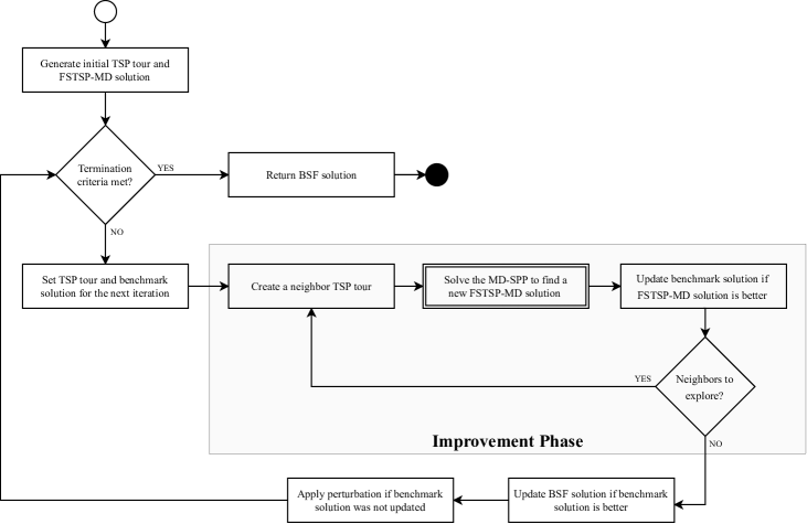
Figure 2: High-level description of the MD-SPP-H.

4.2 The Multi-Drop Shortest Path Problem (Split Algorithm)

The core component of MD-SPP-H is the MD-SPP, which maps a TSP tour into a feasible FSTSP-MD solution in polynomial time. To thoroughly explain the MD-SPP, we start by motivating its conceptualization. We then formally define the MD-SPP and analyze its computational complexity. Throughout this section, we denote $N^{\prime}=N\cup\{0\}$ as the set of nodes, where $0$ is the depot and $N=\{1,...,n\}$ is the set of customers.

The conceptualization of the MD-SPP was inspired by the work of Kundu et al. [2021], who developed a split algorithm for the FSTSP (i.e., the single-drop scenario) that finds an optimal FSTSP solution for a given TSP tour in $\mathcal{O}(n^{3})$ time. Generally speaking, this split algorithm works as follows: first, it generates a weighted directed acyclic graph by enumerating all forward-moving arc times and then finds the shortest path in the generated graph (see A for further details).

Extending the shortest path approach presented in Kundu et al. [2021] for the FSTSP-MD requires enumerating all forward-moving arc times for multiple drops. For a given TSP tour, performing this complete enumeration requires $\mathcal{O}(2^{n})$ time (see Proposition 2 of A), rendering it impractical to solve realistically-sized FSTSP-MD instances. Therefore, to formulate a polynomial-time split algorithm that can be efficiently nested in a local search scheme, we introduce an eligibility criterion to enumerate only a subset of forward-moving arc times, albeit at the expense of “missing” some solutions that are examined when performing a complete enumeration. However, as we will discuss later, it can be argued that efficient local search and perturbation techniques can still visit those solutions that are intentionally omitted.

Our eligibility criterion can be interpreted as imposing an additional constraint on the problem of finding an optimal FSTSP-MD solution for a given TSP route. Specifically, we enforce that the drone can only visit customers immediately following each potential launch node (the rest of the possible drone operations are considered ineligible). More formally, we introduce the concept of partition node, which is defined below.

Definition 1.

(Partition node) Let $\sigma=(0,1,...,n,n+1)$ be a TSP tour whose nodes have been re-indexed based on their positions (where $0$ and $n+1$ denote the depot). Given a subsequence $\sigma^{\prime}_{ij}=(i,i+1,...,j-1,j)$ of $\sigma$, node $k\in N$ (with $i\leq k<j$) is called a partition node if the drone can be launched at node $i\in N^{\prime}$, perform the route $(i+1,i+2,...,k-1,k)$, and be recovered at node $j\in N^{\prime}$, while the truck performs the route $(i,k+1,...,j-1,j)$. When $k=i$, the drone is carried by the truck throughout the entire subsequence.

Illustrative example

Consider an instance of eight customers, as the one shown in Figure 1. Further, consider the TSP tour $\sigma=(0,1,...,8,0)$ and the subsequence $\sigma^{\prime}_{48}=(4,5,6,7,8)$, where Node 4 is the launch node and Node 8 is the recovery node. The enumeration of all potential truck and drone routes (between Node 4 and Node 8) is listed in Table 1. Assuming a sufficiently large drone flight endurance and payload capacity, our MD-SPP only examines those alternatives for which a partition node exists. However, note that the omitted alternatives are examined for neighboring TSP tours of $\sigma$ listed in the last column of Table 1 (these neighboring TSP tours can be readily generated by applying our local search operators over $\sigma$; see Section 4.3).

Table 1: Illustrative example of the effects of using partition nodes for a subsequence $(4,5,6,7,8)$.

Drone route	Truck route	Partition node	Examined?	If not, in which TSP tour is it examined?
Carried by the truck	$(4,5,6,7,8)$	4
$(4,5,8)$	$(4,6,7,8)$	5
$(4,6,8)$	$(4,5,7,8)$	–	–	$(0,1,2,3,4,6,5,7,8,0)$
$(4,7,8)$	$(4,5,6,8)$	–	–	$(0,1,2,3,4,7,5,6,8,0)$
$(4,5,6,8)$	$(4,7,8)$	6
$(4,5,7,8)$	$(4,6,8)$	–	–	$(0,1,2,3,4,5,7,6,8,0)$
$(4,6,7,8)$	$(4,5,8)$	–	–	$(0,1,2,3,4,6,7,5,8,0)$
$(4,5,6,7,8)$	$(4,8)$	7

Now, we formally define the MD-SPP in Problem 1. Using the illustrative example of Section 2, if the underlying TSP tour is $\sigma=(0,1,...,8,0)$, the collection of tuples defined in Problem 1 is given by $P=\{((0,1,2,3),1),((3,4),3),((4,5,6,7,8),7),((8,0),8)\}$, which represents the feasible FSTSP-MD solution shown in Figure 1.

Problem 1.

(The Multi-Drop Shortest Path Problem) Let $\sigma=(0,1,...,n,n+1)$ be a TSP tour whose nodes have been re-indexed based on their positions. The MD-SPP aims to find a collection of tuples $P=\{(\sigma^{\prime}_{i_{0},i_{1}},k_{0}),(\sigma^{\prime}_{i_{1},i_{2}},k_{1}),...,(\sigma^{\prime}_{i_{j},i_{j+1}},k_{j}),...,(\sigma^{\prime}_{i_{\ell},i_{\ell+1}},k_{\ell})\}$ such that (i) $k_{j}$ is a partition node of subsequence $\sigma^{\prime}_{i_{j},i_{j+1}}$, for all $j\in\{0,...,\ell\}$, (ii) the subsequences of $P$ form the TSP tour, and (iii) the completion time is minimized.

Based on the notation listed in Table 2, Algorithm 1 presents a $\mathcal{O}(n^{3})$–time procedure to find the optimal value of Problem 1 (i.e., the completion time at node $n+1$). Broadly speaking, for a given TSP tour $\sigma$ (with nodes re-indexed based on their positions), Algorithm 1 solves the MD-SPP by sequentially computing arc times $c_{i,j}$ for each subsequence $\sigma^{\prime}_{ij}=(i,...,j)$ through Equations (1) and Equation (2):

$$c_{i,j}^{k} =\begin{cases}\displaystyle\sum_{m=i}^{j-1}t_{m,m+1},&\text{if }k=i,\\ \max\left\{\displaystyle\sum_{m=i}^{k-1}d_{m,m+1}+d_{k,j}\>,\>t_{i,j}\right\},&\text{if }k>i,\>j=k+1,\\ \max\left\{\displaystyle\sum_{m=i}^{k-1}d_{m,m+1}+d_{k,j}\>,\>t_{i,k+1}+\sum_{m=k+1}^{j-1}t_{m,m+1}\right\},&\text{otherwise},\end{cases}$$ (1)

$$c_{i,j} =\min\{c_{i,j}^{k}:i\leq k<j,k\leq i+D,c_{i,j}^{k}\leq E\},$$ (2)

where $c_{i,j}^{k}$ represents the arc time if node $k$, with $i\leq k<j$, partitions subsequence $\sigma^{\prime}_{ij}$.

Table 2: Notation used in Algorithm 1.

Symbol	Description
$T_{i}$	Completion time at node $i$, with $i\in\{0,...,n+1\}$.
$t_{i,j}$	Truck travel time from node $i$ to $j$.
$d_{i,j}$	Drone travel time from node $i$ to $j$.
$c_{i,j}^{k}$	Coordinated time taken by the truck and drone to travel from node $i$ to $j$, with partition node $k$.
$D$	Maximum number of drops the drone can perform between launch and recovery.
$E$	Maximum drone flight endurance (in time units).
$a_{i}$, $\alpha_{\text{D}}$, $\alpha_{\text{T}}$	Auxiliary variables to calculate arc times iteratively.
$[i,j]$	Set of integers between $i$ and $j$ (both included), i.e., $[i,j]=\{i,...,j\}$.

Input : TSP tour $\sigma=(0,1,...,n,n+1)$ with nodes re-indexed based on their positions.

Output : Completion time, i.e., $T_{n+1}$.

1 $T_{0}\leftarrow 0$ and $T_{i}\leftarrow\infty,\forall i\in[1,n+1]$

2 for $i\in[0,n]$ do

3       $a_{i}\leftarrow 0$

4       if $T_{i}+t_{i,i+1}$ < $T_{i+1}$ then

5             $T_{i+1}\leftarrow T_{i}+t_{i,i+1}$ $\triangleright$ Relaxation step

6            

7      for $k\in[i+1,\min\{i+D,n\}]$ do

8             $a_{i}\leftarrow a_{i}+d_{k-1,k}$

9             for $j\in[k+1,n+1]$ do

10                   $\alpha_{\text{D}}\leftarrow a_{i}+d_{k,j}$

11                   if $j=k+1$ then

12                         $\alpha_{\text{T}}\leftarrow t_{i,j}$

13                        

14                  else

15                         $\alpha_{\text{T}}\leftarrow\alpha_{\text{T}}+t_{j-1,j}$

16                        

17                  $c_{i,j}^{k}\leftarrow\max\{\alpha_{\text{T}},\alpha_{\text{D}}\}$

18                   if $T_{i}+c_{i,j}^{k}<T_{j}$ and $c_{i,j}^{k}\leq E$ then

19                         $T_{j}\leftarrow T_{i}+c_{i,j}^{k}$ $\triangleright$ Relaxation step

20                  

21            

22      

Algorithm 1 Algorithm to solve Problem 1.

Proposition 1.

For a given TSP tour, Algorithm 1 solves Problem 1 in $\mathcal{O}(n^{3})$ time.

Proof.

See proof in A. ∎

4.3 Exploration of the TSP Solution Space

This section describes how MD-SPP-H explores the TSP solution space. We start by describing the procedures for generating the initial solution and the neighborhoods. We then present the perturbation mechanisms that allow MD-SPP-H to escape local optima and explore unexplored regions of the solution space.

Generation of the initial solution

To create the initial TSP tour, we use the Concorde solver of Applegate et al. [2006] (using the QSopt callable library) to obtain an optimal TSP tour. The initial FSTSP-MD solution is then generated by solving the MD-SPP. This FSTSP-MD solution is designated as the BSF solution and the benchmark solution for the first iteration of MD-SPP-H.

Neighborhood generation

In the improvement phase, we use a composite neighborhood obtained by sequentially applying simple local search operators over the current TSP tour. Specifically, similar to Agatz et al. [2018], we first apply a one-point (1-p) operator (also known as relocate operator; see Savelsbergh [1992]), where a customer is relocated to another position within the current TSP tour; then a two-point (2-p) operator, where two customers are swapped; and finally, the 2-opt operator, where two arcs are removed and replaced with two new ones. Note that the entire exploration of each of these neighborhoods requires $\mathcal{O}(n^{2})$ time. While exploring these neighborhoods, the benchmark solution is updated whenever a new FSTSP-MD solution with a better objective value is found.

After exploring the entire composite neighborhood of the current TSP tour, we update the BSF solution with the benchmark solution if the latter is better. Further, we maintain the benchmark solution for the next iteration if it was updated during the improvement phase (in this case, the TSP tour of the benchmark solution is also set as the TSP tour for the next iteration). Otherwise, we set the benchmark solution and the TSP tour for the next iteration according to the perturbation phase.

Perturbation phase

A critical component in designing an effective heuristic approach involves incorporating diversification (or perturbation) mechanisms to guide the search into previously unexplored regions within the solution space. As previously mentioned, we enter the perturbation phase if the benchmark solution is not updated during the improvement phase.

First, we perform a small perturbation to the current TSP tour by randomly selecting two subsequences from the tour, reversing their orders, and reintegrating them into their original positions (two sequential 2-opt moves). Then, whenever $\eta$ iterations have been conducted without improvement, we perform another diversification mechanism. Here, we first restart the search from the TSP tour of the BSF solution. We then perform the aforementioned reversal of two subsequences followed by randomly relocating the customers of the TSP tour with probability $p$ (which could be considered as applying a mutation operator). After modifying the current TSP tour, we solve the MD-SPP and the corresponding FSTSP-MD solution is set as the benchmark solution for the next iteration.

5 Heuristic Performance

This section presents extensive computational experiments to show the performance of MD-SPP-H. MD-SPP-H was implemented in Java 8 on a scientific HPC cluster. The computational nodes have Intel Xeon CPU E3-1284L v4 processors, each featuring four cores (1.19 GHz nominal, 3.8 GHz peak). The nodes operated on an x86_64 architecture. Based on preliminary experiments, we set $\eta=10$ and $p=0.1$ in the perturbation phase of MD-SPP-H (see Section 4.3). Further, as termination criteria, we stop MD-SPP-H after 200 consecutive iterations without improvement or after a given time limit (described later), whichever comes first. For the interested reader, we provide all problem instances used and detailed results in our GitHub repository at link blinded for peer review.

We focus on realistically sized instances with 50 or more customers (see, e.g., Holland et al. [2017]). Due to the inherent complexity of these instances, comparing MD-SPP-H with exact solution approaches is not possible (see Section 3). Instead, we conduct a pairwise comparative analysis against other state-of-the-art heuristics developed for the FSTSP-MD and the FSTSP (i.e., the single-drop scenario). Despite MD-SPP-H being tailored for multiple drops per drone sortie, we also evaluate its performance on the FSTSP for a comprehensive understanding.

For benchmark purposes, we consider the following solution approaches representative of the current academic state-of-the-art: (i) the IGH of Gonzalez-R et al. [2020] for the FSTSP-MD; (ii) the ALNS of Windras Mara et al. [2022] for the FSTSP-MD; (iii) the Exact Partitioning – All (three local searches) (EP-All) heuristic of Agatz et al. [2018] for the FSTSP; and (iv) the Shortest Path Problem – All (three local searches) (SPP-All) heuristic of Kundu et al. [2021] for the FSTSP.

To enable a fair and consistent comparison, we adhere to the maximum run times allowed and the number of independent runs specified in each benchmark study. We compute two main metrics for our comparison (detailed results for each instance can be found in our aforementioned GitHub repository). First, the relative percentage difference between the best objective values found by each heuristic ($\Delta_{\text{best}}$) is given by

$$\Delta_{\text{best}}=\frac{z^{\text{bench}}_{\text{best}}-z^{\text{MD-SPP-H}}_{\text{best}}}{z^{\text{bench}}_{\text{best}}}\times 100,$$

where $z^{\text{bench}}_{\text{best}}$ and $z^{\text{MD-SPP-H}}_{\text{best}}$ are the best values reached by the benchmark and MD-SPP-H heuristics (across all runs), respectively. Second, the relative percentage difference between the average objective values found by each heuristic ($\Delta_{\text{avg}}$) is given by

$$\Delta_{\text{avg}}=\frac{z^{\text{bench}}_{\text{avg}}-z^{\text{MD-SPP-H}}_{\text{avg}}}{z^{\text{bench}}_{\text{avg}}}\times 100,$$

where $z^{\text{bench}}_{\text{avg}}$ and $z^{\text{MD-SPP-H}}_{\text{avg}}$ are the average values reached by the benchmark and MD-SPP-H heuristics (across all runs), respectively.

Note that EP-All and SPP-All are deterministic; therefore, these heuristics are executed only once. However, we ran MD-SPP-H ten independent times to ensure the robustness of our results. We adjust our aforementioned metrics accordingly and compare both our best and average results to the single solution value reached by the respective method. Finally, in B, we also include an additional comparison with the integer L-shaped method of Vásquez et al. [2021] over small FSTSP instances with up to 20 customers.

5.1 Comparison with state-of-the-art solution approaches for the FSTSP-MD

This section begins by comparing the performance of MD-SPP-H with the seminal IGH of Gonzalez-R et al. [2020]. We then extend our analysis to compare MD-SPP-H with the recent ALNS heuristic proposed by Windras Mara et al. [2022].

Comparison with the IGH of Gonzalez-R et al. [2020]

To test their heuristic, Gonzalez-R et al. [2020] use the popular problem instances originally introduced by Agatz et al. [2018]. We select instances from the dataset with 50 up to 250 customer locations. The spatial distribution of these locations follows three distinct patterns: uniform, single-centered, and double-centered. The benchmark set contains 10 instances for each node count and distribution pattern. Travel times for both the truck and drone are based on Euclidean distances. Service time, as well as launch and recovery duration, are not considered. Lastly, all customers can be either served by the truck or the drone (i.e., all customers are drone-eligible).

As described in Section 3, Gonzalez-R et al. [2020] assume the drone can perform as many drops as its flight endurance allows (i.e., no constraints limit the total number of separate packages the drone can deliver per sortie). In our MD-SPP-H, this assumption can be readily incorporated by removing the maximum number of drone drops constraint in Algorithm 1 (or, equivalently, by setting $D=n$). The maximum flight endurance is assumed proportional to the average drone travel time between the nodes, represented as $E=\frac{2}{n\cdot(n+1)}\sum_{(i,j)\in A}d_{i,j}$ (where $A$ denotes the set of arcs between the nodes). To ensure a precise comparison, we use the same maximum flight endurance values as Gonzalez-R et al. [2020].

Finally, Gonzalez-R et al. [2020] impose a maximum time limit of 600 seconds for IGH, which we also use as a termination criterion for MD-SPP-H. Table 4 in B summarizes the experiment setting. We also refer the reader to our GitHub repository for details on the actual run times required by MD-SPP-H and IGH.

Before presenting the comparison between both heuristics, it is worth mentioning that IGH assumes that the truck-and-drone delivery system starts at the depot but ends at the last customer listed in Agatz et al. [2018]’s instances. Consequentially, IGH does not consider the time for the vehicles to return to the depot after serving the last customer listed. In contrast, MD-SPP-H aims to minimize the completion time of the delivery process (i.e., the time when the last vehicle returns to the depot), consistent with most drone logistics studies (see, e.g., Chung et al. [2020]). Therefore, the comparison presented below considers that MD-SPP-H finishes at the depot while IGH at the last customer listed in Agatz et al. [2018]’s instances. However, it could be argued that the time to return to the depot may be negligible for instances with more than 50 customers.

Figure 3 presents the results for instances with uniformly distributed locations, considering three different drone speed ratios (i.e., the ratio of the drone speed to the truck speed). Results show that MD-SPP-H outperforms IGH in terms of solution quality. Overall, MD-SPP-H improves the best solution values found ($\Delta_{\text{best}}$) by 25.3%, 12.5%, and 8.0% (average over all instances) for drone speed ratios of 1, 2, and 3, respectively, while improving the average solution value ($\Delta_{\text{avg}}$) by 27.4%, 12.5%, and 7.3%. The most significant relative enhancements occur when the drone operates at slower speeds (i.e. when its speed is the same as that of the truck). Based on the quality measures reported in Gonzalez-R et al. [2020], we observe that IGH seems to lead to more consistent results as drone speed increases, regardless of customer distribution. Lastly, we refer the reader to our GitHub repository for detailed results on single- and double-center instances. Results show that MD-SPP-H outperforms IGH regardless of the customer distribution. However, we observe that the percentage improvements for the non-uniform distributions are slightly smaller. For a drone speed ratio of 1 and averaged over all instances, we observe values for $\Delta_{\text{best}}$ of 17% and 21.3% for single- and double-center distribution, respectively.

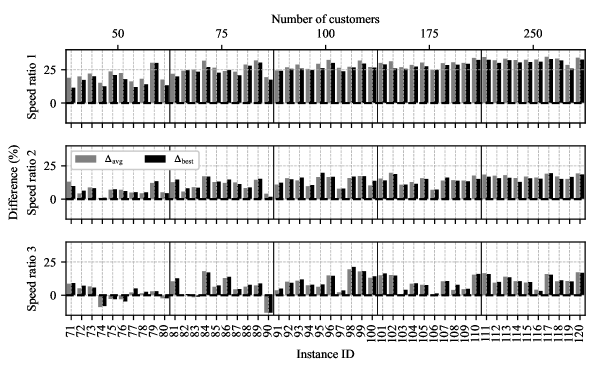
Figure 3: Relative percentage differences between MD-SPP-H and IGH (based on the solution published by Gonzalez-R et al. [2020]), considering 50, 75, 100, 175, and 250 uniformly distributed customers.

Comparison with the ALNS of Windras Mara et al. [2022]

We now compare the performance between MD-SPP-H and ALNS using one of the three datasets used by Windras Mara et al. [2022] made available to us. This dataset, initially introduced by Ha et al. [2018] for the single-drop scenario, comprises 60 benchmark instances with 50 and 100 customers. Instances named B1-B10, C1-C10, and D1-D10 contain 50 uniformly distributed customers across service areas spanning 100, 500, and 1,000 km², respectively. Additionally, instances labeled E1-B10, F1-C10, and G1-D10 consist of 100 uniformly distributed customers across the same area dimensions. Readers can refer to Ha et al. [2018] for a more detailed description of these instances. It is important to notice that, for all instances, 20% of the customers chosen randomly are designated as ineligible for drone delivery (i.e., these customers must be served by the truck). We adjusted MD-SPP-H to accommodate this additional constraint (by restricting that all customers between node $i$ and node $k$ in Algorithm 1 must be drone-eligible). Further, truck distances are calculated based on the Manhattan metric, while drone distances are determined using the Euclidean metric. Windras Mara et al. [2022] set both the truck and the drone speed to 40 km/h. The drone flight endurance is set to 24 minutes, and the time required for the truck to launch and retrieve the drone is 30 and 40 seconds, respectively. During the launch and retrieval phases, the drone is assumed to be in a non-flight mode, eliminating the need to factor this time into flight endurance consumption. Moreover, since Windras Mara et al. [2022] assume that the drone load capacity is unlimited, we set $D=n$ in Algorithm 1. Finally, to ensure a fair comparison and align with the computation times reported by Windras Mara et al. [2022], we use maximum run times of 60 and 90 seconds for instances with 50 and 100 customers, respectively. We further adopt the same number of independent runs (i.e., 10 runs). For a summary of our experiment settings, please refer to Table 4 in B.

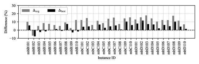
Figure 4: Relative percentage differences between MD-SPP-H and ALNS, considering 50 customers and the B, C, D service area sizes of Ha et al. [2018].

Figure 4 and 5 report the results for instances with 50 and 100 customers, respectively. Overall, MD-SPP-H improves the best solution found by ALNS by $\Delta_{\text{best}}=3.5\%$ for instances with 50 customers and by $\Delta_{\text{best}}=8.0\%$ for instances with 100 customers. The improvements are even more pronounced for the average solution values, with average improvements of $\Delta_{\text{avg}}=10.3\%$ and $\Delta_{\text{avg}}=15.7\%$ for instances with 50 and 100 customers, respectively. This behavior is because MD-SPP-H produces more consistent results than ALNS in terms of standard deviation values across the ten independent runs (see our aforementioned GitHub repository for further details). For example, ALNS reports standard deviations of 13.3 and 22.0 (time units) for instances of 50 and 100 customers, respectively, while MD-SPP-H exhibits much lower standard deviations of 2.2 and 2.6 (time units). Finally, our results show a tendency for greater improvements in instances with larger service areas, particularly in instances D and G (i.e., 1,000 km²).

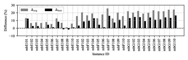
Figure 5: Relative percentage differences between MD-SPP-H and ALNS, considering 100 customers and the E, F, G service area sizes of Ha et al. [2018].

5.2 Comparison with state-of-the-art solution approaches for the FSTSP

To further analyze the performance of MD-SPP-H, we perform an additional benchmark with three solution approaches tailored for the FSTSP (i.e., the single-drop scenario): the established EP-All heuristic of Agatz et al. [2018], the SPP-All heuristic of Kundu et al. [2021], and the integer L-shaped method of Vásquez et al. [2021]. All comparisons are based on the uniform instances of Agatz et al. [2018] (extended by Vásquez et al. [2021] for problem sizes of $n\in\{11,...,20\}$ customers). For the comparison with EP-All and SPP-All, we use the results that are available on Kundu et al. [2020], while the best-known values provided by Vásquez et al. [2021] are used to compare MD-SPP-H with their integer L-shaped method. In all benchmarks, the drone’s speed is assumed to be double that of the truck, and the drone’s maximum flight endurance is considered unlimited. We summarize the experiment setting in Table 4 in B.

Comparison with EP-All and SPP-All

Our comparative analysis with the heuristics developed by Agatz et al. [2018] and Kundu et al. [2021] is depicted in Figures 6 and 7, respectively. First, Figure 6 clearly demonstrates that MD-SPP-H significantly improves solution quality compared to EP-All, with similar or reduced run times. The reduction in runtime is noticeable for large instances with 175 and 250 customers. In terms of solution quality, MD-SPP-H improves the best-found solution value by $\Delta_{\text{best}}=4.9\%$ (average over the 50 instances). The percentage improvements are particularly high for instances with 75 and 100 customers. The average solution value reached by MD-SPP-H improves the solution found by EP-All by $\Delta_{\text{avg}}=3.3\%$ (average over the 50 instances). Therefore, MD-SPP-H outperforms EP-All in terms of both solution quality and computational efficiency.

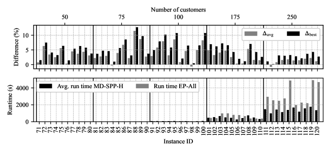
Figure 6: Benchmark of MD-SPP-H with solution published by Agatz et al. [2018]: uniform distribution and at least 50 customers.

Second, we compare our results with the SPP-All heuristic of Kundu et al. [2021]. The notable advancement in their study, compared to Agatz et al. [2018], is the significant reduction in computation time while maintaining or slightly improving solution quality. For instance, SPP-All requires an average run time of 43.4 seconds for instances with 250 customers. Regarding solution quality, Kundu et al. [2021] report achieving an overall mean improvement of 0.77% over EP-All (in contrast, MD-SPP-H improves the overall solution quality by $\Delta_{\text{best}}=4.9\%$ and $\Delta_{\text{avg}}=3.3\%$).

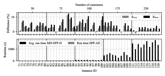
Figure 7: Benchmark of MD-SPP-H with solution published by Kundu et al. [2021]: uniform distribution and at least 50 customers.

Figure 7 shows that MD-SPP-H improves the best solution found for almost all instances. Specifically, MD-SPP-H improves the best solution values found by $\Delta_{\text{best}}=4.3\%$ (average over all instances with uniform customer distribution), with a notable peak improvement of $\Delta_{\text{best}}=5.8\%$ (average over the 10 instances) for instances with 100 customers. Further, $\Delta_{\text{best}}$ is negative in only two out of 50 instances (i.e., SPP-All outperforms MD-SPP-H). Across all instances, the average solution value reached by MD-SPP-H improves the best-known solution found by SPP-All by $\Delta_{\text{avg}}=2.7\%$, and we obtain slightly worse results for only seven out of 50 instances.

Regarding run times, MD-SPP-H requires an average of 5 seconds for instances with 50 customers, while an average of 71 seconds for instances with 100 customers. For instances with 250 customers, the average run time of MD-SPP-H is around 23 minutes. While these run times significantly exceed those achieved by the SPP-All heuristic of Kundu et al. [2021] (as depicted in Figure 7), they remain reasonable when considering the FSTSP-MD’s inherent complexity. The reader can refer to Figure 11 in B for additional information on the relative percentage difference (over time) between the best-so-far solution and the best overall solution found by MD-SPP-H. For example, for instances with 250 customers, the solutions found by MD-SPP-H after 10 minutes are within 4% of the best overall solutions. For real-world applications, this implies that last-mile logistics managers could execute MD-SPP-H for just a couple of minutes and get high-quality solutions.

Comparison with the integer L-shaped method of Vásquez et al. [2021]

Finally, we compare MD-SPP-H with the integer L-shaped method developed by Vásquez et al. [2021]. (Recall that a meaningful comparison for the FSTSP-MD is not possible as existing exact approaches can only address instances of up to eight customers; see Section 3.) This exact method finds optimal solutions for FSTSP instances with up to 20 customers. Table 5 in B reports the comparison using the best-known values provided by Vásquez et al. [2021]. Overall, MD-SPP-H solves to optimality 73 out of the 88 instances that the integer L-shaped method solves to optimality. Further, the average run time of MD-SPP-H is less than half a second. Finally, for instances with more than 17 customers, MD-SPP-H improves the best solutions found by the integer L-shaped method by 1.4%.

In summary, although designed for the multi-drop scenario, MD-SPP-H marks a substantial step forward in improving solution quality for the FSTSP while maintaining practical run times.

6 Impact of Individual Parameters and Their Interaction on Time Savings and Delivery System Performance

In Section 5, we showed the superior performance of MD-SPP-H compared to state-of-the-art solution approaches for both the FSTSP-MD and the FSTSP. In this section, we leverage our proposed solution approach to improve our understanding of collaborative truck-and-drone delivery systems for last-mile logistics. We aim to advance the understanding of the benefits and drawbacks of cooperative truck-and-drone delivery systems. Throughout this section, we use the parameter values of $\eta=10$ and $p=0.1$ (used in the perturbation phase of MD-SPP-H) and the computational setting described in Section 5.

6.1 Design of Numerical Experiments

For the analyses presented in this section, we rely on the well-established FSTSP instances from Agatz et al. [2018]. We replicate the conditions in their study by adhering to the following assumptions. For all scenarios, both the truck and the drone travel the Euclidean distance between the nodes, and the truck travels at a unit speed. Customer service times and drone launching and recovery times are negligible [see also, e.g., Gonzalez-R et al., 2020].

Baseline Scenario

We establish a baseline scenario following the one chosen by Agatz et al. [2018] for the single-drop case. We select instances with 100 uniformly distributed customers within the service area. The drone travels at twice the speed of the truck, and we consider an unlimited drone flight endurance. In line with current multi-drop drones, such as the A2Z Drone Delivery [Sakharkar, 2021], we set the baseline maximum number of drone drops to $D=2$.

Scenarios of Analysis

Building on this baseline, we analyze the effects of varying the following input parameters: the maximum number of drone drops, the drone speed ratio (compared to the truck speed), the drone’s maximum flight endurance, and the number and geographical distribution of the customers. In total, our experiment design gives rise to 9,000 scenarios, i.e., unique parameter combinations. For each scenario, we include ten instances (i.e., we solve a total of 90,000 instances). A summary of our experiment design is presented in Table 3. In the following, we explain our parameter choices.

1) Number of drone drops

We systematically vary the number of drone drops within $D\in\{1,2,4,6,10\}$ to capture potential practical limitations of drone payload capacity, whether due to weight or equipment constraints. Note that we also include the case of a single-drop drone to facilitate a direct comparison of our findings with previous studies.

2) Drone speed ratio

Starting with a baseline drone speed ratio (i.e., the ratio of the drone speed to the truck speed) of 2, we decrease and increase the ratio to 1 and 3, respectively. These drone speed ratios are used in several prior studies [see, e.g., Gonzalez-R et al., 2020, Roberti & Ruthmair, 2021, Schermer et al., 2019b].

3) Drone flight endurance

Through preliminary experiment runs, we identified 100 time units as an effectively unlimited drone flight endurance level (when all remaining parameters take their baseline values). Starting with 100 time units as the upper limit, we decrease the drone flight endurance in steps of 25 time units, exploring values down to 25 time units. These values are chosen to cover a wide range of restriction levels. A comparison between actual flight duration and maximum flight endurance across all scenarios with uniform customer distribution, as shown in Figure 10, reveals that our chosen range extends from unrestricted to notably restricted drone flight endurance.

4) Number and 5) distribution of the customers

As provided in the full dataset by Agatz et al. [2018], the number of customers within the service area varies between 50 and 250 customers. Further, in addition to the uniform customer distribution, we also consider instances with single-center and double-center customer distributions. Note that instances with uniform customer distributions are limited to a service area of $100\times 100$ distance square units, resembling highly dense urban settings. In contrast, instances with single-center and double-center customer distributions cover approximately $300\times 300$ and $500\times 300$ distance square units, respectively. These configurations may resemble less dense service areas where customers are concentrated around one or two central locations.

Table 3: Summary of parameter choices for numerical experiments on problem instances from Agatz et al. [2018]

Type	Parameter	Value
General	Total number of instances	150
	Customer distribution	Uniform∗, single-center, double-center
	Number of customers	$\{50,75,100^{*},175,250\}$
Vehicle	Drone eligibility	100%
	Truck distance	Euclidean [unit]
	Drone distance	Euclidean [unit]
	Truck speed	1
	Drone speed ratio	$\{1,2^{*},3\}$
	Flight endurance	$\{25,50,75,100^{*}\}$
	Number of drops	$\{1,2^{*},4,6,10\}$
	Launch/retrieval time	0/0
CPU	Run-time limit	10 min (for $n\leq 100$), 30 min (for $n\geq 175$)
	Runs	5
Note. * denotes values used in the baseline scenario.

For each scenario, we evaluate the performance of the cooperative truck-and-drone system compared to the truck-only system. By default, we calculate the percentage of completion time savings as

$$\Delta=\frac{z^{\text{TSP}}-z^{\text{MD-SPP-H}}}{z^{\text{TSP}}}\times 100,$$

where $z^{\text{TSP}}$ is the completion time of the truck-only delivery system obtained by the Concorde solver [Applegate et al., 2006] and $z^{\text{MD-SPP-H}}$ is the completion time of the truck-and-drone delivery system obtained by MD-SPP-H. If not indicated otherwise, we report the average time saving over the ten instances for each scenario.

6.2 Direct Effects

For our baseline parameter setting (see Section 6.1), the truck-and-drone system yields average completion time savings of 41.6% compared to the truck-only system (see Figure 8(a) for two drops). In the following, we first discuss the direct effects of the three drone operational parameters on the delivery system’s performance. Second, we investigate how each of the service area’s characteristics, i.e., the number and distribution of customers, affect the time savings.

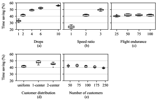
Figure 8: Percentage of time savings for ten problem instances, obtained by varying a single parameter from our baseline scenario.

Altering the number of drone drops

Figure 8(a) confirms that the truck-and-drone delivery system can significantly reduce the total duration of the delivery process compared to the truck-only system. The percentage of time savings increases as the drone makes more drops, starting from 33% savings for a single-drop drone up to 56% for a drone capable of up to ten drops. However, our results show that this relationship is not linear, but is characterized by rapidly diminishing marginal returns as the number of drops increases.

Altering the drone speed ratio

Not surprisingly, the relative speed of the drone compared to the truck emerges as a critical factor influencing the achievable time savings over the truck-only scenario. For the baseline drone speed ratio of 2, Figure 8(b) shows attainable completion time savings of 41.6%. This value decreases to savings of 24.1% for a speed ratio of 1, and increases to 49.6% for a speed ratio of 3. Again, we observe diminishing marginal returns as the speed ratio increases. This is likely due to the need for coordination between truck and drone movements. In other words, if we only increase the drone’s speed while keeping the other system parameters fixed, the drone will have to wait for the truck more frequently and for longer periods, limiting the potential for system-level completion time savings. Note that this finding is consistent with conclusions that Agatz et al. [2018] obtained for the single-drop case.

Altering the drone flight endurance

Intuitively, a sufficiently high drone flight endurance allows the system to reap the full potential of time savings offered by combining trucks and drones for last-mile logistics. Conversely, the potential time savings are diminished if the drone’s ability to move independently is limited due to limited flight endurance. For instance, Figure 8(c) shows a reduction in time savings by 1.5% as the flight endurance level drops to 25 time units. For endurance levels of 50 and higher, this parameter does not impact the time savings, i.e., the savings plateau. This implies that, while meeting a certain flight endurance threshold is essential to leveraging the full efficiency gains, further improvement beyond this saturation point yields no additional benefits. While this effect is almost negligible in our baseline scenario, it is more pronounced for other parameter combinations. We refer to our discussion in Section 6.3.

Non-uniform customer distributions

Figure 8(d) shows that the truck-and-drone delivery system achieves substantial savings over different customer distributions. The average time savings increase from 41.6% (reached over uniform instances) to 47.7% and 45.1% for single- and double-center instances, respectively. This implies that drones are more advantageous when serving distribution areas where customers are concentrated around a few central locations, with only a small number of customers located in outlying regions. As Agatz et al. [2018] highlights for single-drop drones, a plausible explanation is that the drone supports the truck by serving customers furthest from the center of the cluster(s) efficiently.

Altering the number of customers

As we vary the number of customers between 50 and 250, the relative time savings vary between 39.2% and 42.8% (see Figure 8(e)). However, our results do not reveal a clear and unambiguous relationship between the number of customers and the obtainable time savings (similar results were obtained for the single- and double-center customer distributions). For our baseline scenario, relative time savings remain relatively stable despite significant changes in the number of customers. This implies that customer density plays a minor role in the benefits achieved by the truck-and-drone system (an observation that, of course, highly relies on the chosen baseline parameters). Therefore, we conduct an additional investigation in Section 6.3 to examine this effect in more detail.

6.3 Parameter Interactions

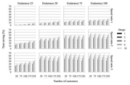
Figure 20: Average percentage time savings over ten problem instances from a truck-and-drone system compared to the truck-only alternative for varying parameter settings and single-center customer distribution.

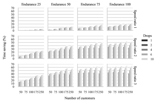
Figure 23: Average percentage time savings over ten problem instances from a truck-and-drone system compared to the truck-only alternative for varying parameter settings and double-center customer distribution.

Having examined how every single parameter impacts the dynamics of the delivery system and the resulting relative time savings, we further investigate how these effects interact. We split this section into two parts. We first discuss the delivery system’s inherent dynamics, i.e., how the three operational drone parameters interact to impact the savings. We then discuss how the operational environment of the collaborative delivery system impacts its inherent dynamics (and consequentially the time savings in a specific use case). To this end, we discuss the dominant patterns emerging from our full factorial experiment data. The results for uniform customer distributions are summarized in Figure 9. Results for single- and double-center customer distributions are presented in Figures 20 and 23 in Online Appendix C, respectively.

Figure 9: Average percentage time savings over ten problem instances from a truck-and-drone system compared to the truck-only alternative for varying parameter settings and uniform customer distribution.

6.3.1 System-Inherent Dynamics

In the following, we explore how different levels of one drone operational parameter affect the impact of changes in another parameter on time savings. We stick to the baseline operational environment of 100 uniformly distributed customers.

Interaction of key drivers of time savings: drone drops and speed ratio

Figure 9 shows that the drone speed ratio significantly moderates the benefits of increasing the number of possible drone drops. For a drone speed ratio of 3 (2, 1), and a baseline endurance of 100 time units, the achievable time savings increase from around 39.8% (33.0%, 18.1%) for a single-drop drone to around 65.0% (56.0%, 36.6%) for a ten-drop drone. This corresponds to an absolute effect of 25.2 (23.0, 18.5) percentage points and a relative increase by approximately 63.3% (69.7%, 102.2%). In other words, the higher the drone speed ratio, the larger the absolute gain but the smaller the relative gain from enabling the drone to make more drops per sortie. This is an intuitive result since a faster drone has a larger time-saving potential to begin with, even in the single-drop case, than a drone that travels at the same speed as the truck.

Flight endurance as a prerequisite for multiple drops

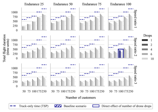
Figure 19: Comparison of average observed total drone flight duration (i.e., sum over all drone flights) over ten instances and truck-only delivery system completion time for instances with uniform customer distribution

A sufficient flight endurance limit is a prerequisite to realizing the efficiency gains of a collaborative delivery system with a multi-drop drone. The benefits of increasing the number of possible drone drops are diminished if the drone’s flight endurance becomes too restrictive. We observe a truncation effect for low flight endurance levels: while we still see measurable benefits from moving from a low number of drops per drone sortie to a slightly higher number, the savings plateau, and no further improvements are obtained beyond a certain number of drops per sortie (see Figure 9 for an endurance level of 25 time units and speed ratio of 2). This effect is more pronounced and sets in at higher levels of flight endurance as the drone speed ratio decreases (see Figure 9 for an endurance level of 50 comparing speed ratios 1 and 2). This is expected because a very restrictive flight endurance keeps the drone from exploiting the ability to make many drops per sortie unless these drops are closely co-located. Further, our analysis reveals a somewhat surprising and valuable insight: the sum of all drone flying times is inversely related to the number of drops that a drone can make per flight (cf., Figure 19 in Online Appendix C). Although the maximum duration of a single drone flight increases with a higher number of drops, we note that the aggregate duration of all drone flights combined decreases as the maximum number of possible drops increases. Allowing the drone to serve multiple customers in one sortie reduces the number of back-and-forth trips performed by the drone between the truck and the customers it serves. As a result, the collaborative system completes its deliveries faster, and the drone uses less total battery power.

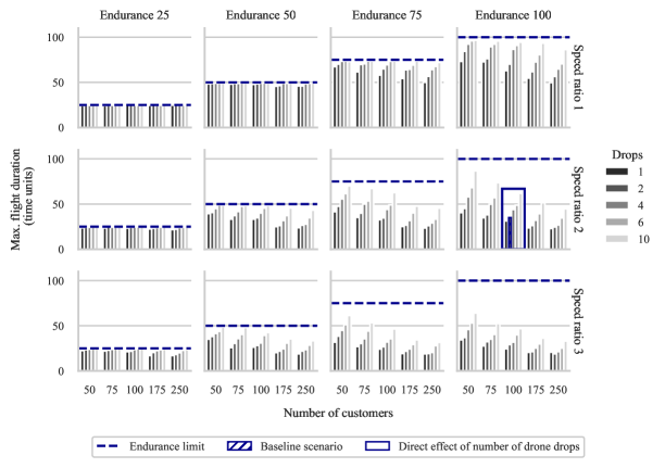
Figure 10: Comparison of average observed maximum drone flight duration over ten instances and imposed drone flight endurance limit for instances with uniform customer distribution.

Compensating effect of drone speed and flight endurance level

Assuming independence of drone speed and flight endurance, the two parameters can compensate for each other if one is overly restrictive. Specifically, a higher drone speed can compensate for a very restrictive flight endurance limit (see Figure 10 for an endurance level of 50 time units and increasing speed ratios). Conversely, boosting flight endurance levels can mitigate the drawbacks of a slower drone (see Figure 10 for a speed ratio of 1 and increasing endurance levels). However, drone flight endurance only indirectly affects time savings; see our discussion on the saturation point in Section 6.2.

6.3.2 Impact of the Operational Environment

The operational environment (i.e., customer density and distribution) significantly affects the distances that the truck and the drone need to travel. For instance, the lower the customer density, the greater the distance between customers, requiring longer drone flight distances. Similarly, transitioning from a uniform to a non-uniform customer distribution increases drone flight distances, as the drone is typically used to predominantly serve remote customers (see Section 6.2). While the potential savings in these scenarios might be particularly high, they can challenge the drone’s flight endurance.

Serving areas with low customer density

For most parameter combinations depicted in Figure 9, the time savings from the truck-and-drone system are independent of the number of customers and, therefore, the customer density. Only for low endurance levels and speed ratios, the achievable time savings quickly diminish as the number of customers decreases, up to the point where virtually no time savings can be obtained (see the top left panel of Figure 9). This suggests that the benefits of adding a multi-drop drone are largely independent of the average distance between customers in the service area as long as the drone’s flight endurance is sufficient and the drone is comparably fast. However, without these requirements, the drone is not able to effectively contribute to reducing delivery completion times in service areas with a low customer density.

Serving areas with non-uniform customer distribution

We first consider scenarios in which the drone is effectively not restricted in flight endurance. In these cases, our results reveal that the impact of increasing the number of drone drops on time savings is consistent across varying customer distributions, that is, we identify the same general pattern of marginal diminishing returns (i.e., similar incremental time savings as the number of drone drops increases). However, the absolute level of time savings is higher in non-uniform compared to uniform customer distribution (cf., Figure 9 and Figures 20, and 23 in Online Appendix C for a flight endurance level of 100 time units and a speed ratio of 3). Interestingly, moving from unrestricted drone movements to more restrictive levels of flight endurance and lower speed ratios, we find that a non-uniform customer distribution might act as a catalyst for the performance effects of changes to these drone operational parameters. As non-uniform distributions demand longer distances per drone flight, the same level of drone flight endurance and speed have a stronger limiting effect in non-uniform than in uniform scenarios, which in turn impacts the potential time savings in these settings.

7 Implications for Practice

The findings from our study of the impact of different parameters on time savings and system performance lead to several implications and recommendations for practitioners and policymakers. First, our work shows that the application of collaborative truck-and-drone delivery systems can significantly reduce total delivery times. Second, our results show that the achievable relative truck distance savings closely mirror the relative time savings, i.e., both metrics take on similar values. As a result, trucks would travel fewer miles and spend less time on the road, reducing emissions and congestion. While the potential savings are considerable, their extent is primarily determined by the characteristics of the service area and available drone technology, underscoring the need for case-dependent evaluations.

Specifically, our analysis indicates that the attainable time savings strongly depend on the speed ratio between the truck and the drone and the maximum number of drops. For both parameters, we observe diminishing marginal returns. We find that single-drop drones or drones capable of making a few drops – which are already available on the market [Sakharkar, 2021, Wingcopter, 2023] – that travel at a moderate speed (e.g., twice the speed of a traditional delivery truck) can lead to significant time savings. For a uniform customer distribution and sufficient flight endurance levels, the time savings from adding a drone that travels at twice the speed of the truck range between 33.1% for a single-drop drone and 48.7% for a drone capable of up to four drops. However, considering the increased technological and operational complexity and costs associated with systems designed for numerous drops (i.e., five or more), a thorough economic assessment based on the specific use case is warranted before adopting and deploying such systems.

Considering the trade-off between investing in increasing either drone speed or the number of possible drops, we find that both input parameters alter the dynamics of the truck-and-drone delivery system in distinct ways, and the incremental improvements will depend on the remaining operational parameters of the drone and the characteristics of the service area. For instance, we find for our baseline scenario that increasing the number of drone drops from two to four yields the same efficiency gains as increasing the drone-to-truck speed ratio from 2:1 to 3:1 (cf. Figure 8(a) and (b)). Therefore, when adopting drone delivery operations, balancing the investment in drone speed against the practical benefits of multiple drops is crucial, focusing on the most cost-effective combination for the specific use case.

Finally, our study can help last-mile delivery companies decide for which operational environments (characterized by the density and spatial distribution of customers) they should consider investing in a truck-and-drone delivery system, and policymakers decide for which environments they should provide the policy framework. We find that the operational environment can act as a stress test for the collaborative system, highlighting the importance of carefully assessing the suitability of the drone’s flight endurance and speed to reach optimal performance for different use cases. For example, we show that potential time savings can be particularly high when serving non-uniformly distributed customers or service areas with low demand density, but enhanced drone capabilities (speed and endurance) are needed to reap the full benefits of the collaborative system.

8 Conclusion

In this paper, we investigate the benefits of combining conventional ground delivery vehicles and aerial cargo drones for last-mile logistics. This approach leverages the numerous advantages of using drones, including their low per-vehicle capital expenditure costs, reduced carbon footprint, and travel directness and speed. Specifically, we explore the value of supporting ground delivery vehicles with drones capable of making multiple package deliveries per sortie.

We study the Flying Sidekick Traveling Salesman Problem with Multiple Drops (FSTSP-MD), a multi-modal last-mile delivery model where a single truck is supported by a single multi-drop drone during the delivery process. In this model, the drone can be launched from the truck en route to make autonomous package deliveries to multiple customers before returning to the truck. The FSTSP-MD aims to determine the synchronized truck and drone delivery routes that minimize the completion time of the delivery process.

We propose the Multi-Drop Shortest Path Problem–Based Heuristic (MD-SPP-H) to solve realistically-sized FSTSP-MD instances. MD-SPP-H is a simple and highly effective order-first, split-second heuristic that combines standard local search and diversification techniques with a novel shortest-path problem that finds FSTSP-MD solutions (for a given order of customers) in polynomial time.

Using well-established instances with between 50 and 250 customers, we show that MD-SPP-H outperforms state-of-the-art heuristics developed for the FSTSP-MD and the FSTSP. Further, compared to the exact solution approach developed by Vásquez et al. [2021] for the FSTSP, we show that MD-SPP-H solves most instances (with up to 20 customers) to optimality in less than half a second, with only a minor average optimality gap of 0.15%. Several managerial insights and policy implications are also presented regarding using drones to boost the efficiency of traditional, ground-based delivery vehicles.

There are several potential avenues for future research. For instance, MD-SPP-H could be extended to allow the truck to launch and recover the drone at locations other than customer nodes (see, e.g., Schermer et al. [2019a]). Further, the FSTSP-MD assumes a constant drone flight speed and a drone battery consumption independent of carrying weight. Thus, future research could enrich our MD-SPP formulation to account for more realistic drone parameters (see, e.g., Jeong et al. [2019] and Raj & Murray [2020]). Finally, a natural extension is to consider multiple trucks equipped with multiple drones.

BOFV

benchmark objective function value

IGH

Iterated Greedy Heuristic

MD-SPP

Multi-Drop Shortest Path Problem

MD-SPP-H

Multi-Drop Shortest Path Problem–Based Heuristic

FSTSP

Flying Sidekick Traveling Salesman Problem

FSTSP-MD

Flying Sidekick Traveling Salesman Problem with Multiple Drops

SPP

Shortest Path Problem

TSP

Traveling Salesman Problem

TSP-D

Traveling Salesman Problem with Drone

MILP

Mixed-Integer Linear Programming

ALNS

Adaptive Large Neighborhood Search

EP-All

Exact Partitioning – All (three local searches)

SPP-All

Shortest Path Problem – All (three local searches)

Appendix A Proof of Propositions

Complexity of split algorithms

To find an optimal FSTSP solution for a given TSP tour, the split algorithm of Kundu et al. [2021] solves the shortest path problem in a weighted directed acyclic graph. Specifically, given the TSP tour $\sigma=(0,1,...,n,n+1)$ (whose nodes have been re-indexed based on their positions), the authors build the graph $\mathcal{G}=(\mathcal{N},\mathcal{A})$, where $\mathcal{N}=\{0,1,...,n,n+1\}$ and $\mathcal{A}=\{(i,j):i\in\mathcal{N}\backslash\{n+1\},j\in\{i+1,...,n+1\}\}$. Each arc $(i,j)\in\mathcal{A}$ is called a forward-moving arc. To solve the shortest path problem, the authors enumerate all forward-moving arc times associated with each $(i,j)\in\mathcal{A}$. Notably, each $(i,j)\in\mathcal{A}$ has associated a maximum of $j-i$ forward-moving arc times, defined by the maximum number of single-drop drone operations between nodes $i$ and $j$ (including the one where the drone is carried by the truck). As Kundu et al. [2021] prove, the complete enumeration of all forward-moving arc times can be done in $\mathcal{O}(n^{3})$ time for the FSTSP. The interested reader can refer to Kundu et al. [2021] for further details.

For the FSTSP-MD, Proposition 2 states that, without the introduction of partition nodes, solving the shortest path problem by enumerating all forward-moving arc times requires $\mathcal{O}(2^{n})$ time.

Proposition 2.

For a given TSP tour, solving the shortest path problem by enumerating all forward-moving arcs requires $\mathcal{O}(2^{n})$ time.

Proof.

Consider the TSP tour $\sigma=(0,1,...,n,n+1)$, whose nodes have been re-indexed based on their positions. Assume that the maximum drone flight endurance constraint is removed. Now consider a subsequence $\sigma^{\prime}_{ij}=(i,i+1,...,j-1,j)$ of the TSP tour $\sigma$, where $i$ is the launch node and $j$ is the recovery node. The total number of operations where the drone performs exactly $m$ deliveries is given by ${j-i-1\choose m}$. Therefore, when we relax the constraint for the maximum number of drone drops, the maximum number of possible drone operations (including the one where the drone is carried by the truck throughout the entire subsequence) is given by $\sum_{m=0}^{j-i-1}{j-i-1\choose m}$ = $2^{j-i-1}$ (representing the total number of forward-moving arc times between nodes $i$ and $j$).

Now, since the TSP tour $\sigma$ has $n+2$ nodes, there is a maximum of $\sum_{i=0}^{n}\sum_{j=i+1}^{n+1}2^{j-i-1}=2^{n+2}-n-3$ possible forward-moving arc times (i.e., coordinated truck-and-drone routes) for the given TSP tour $\sigma$. Therefore, a split algorithm without the introduction of partition nodes requires $\mathcal{O}(2^{n})$ time. ∎

Proof of Proposition 1

Let us introduce Definition 2 and Lemmas 1 and 2 before proving Proposition 1.

Definition 2.

(Optimal partition node) Let $\sigma=(0,1,...,n,n+1)$ be a TSP tour whose nodes have been re-indexed based on their positions. Given a subsequence $\sigma^{\prime}_{ij}=(i,i+1,...,j-1,j)$ of $\sigma$, we refer to node $k^{*}\in N$ as an optimal partition node if $k^{*}\in\operatorname*{arg\,min}_{k}\{c_{i,j}^{k}:i\leq k<j,k\leq i+D,c_{i,j}^{k}\leq E\}$. Therefore, $c_{i,j}=c_{i,j}^{k^{*}}$.

Lemma 1.

(Upper bound) Assume that Algorithm 1 is applied to the TSP solution $\sigma=(0,1,...,n,n+1)$. At any time of the run, for each $j\in\{0,...,n+1\}$, we always have $T_{j}\geq\delta(0,j)$, where $\delta(0,j)$ represents the total time of the true shortest path from node $0$ to node $j$. If we ever find $T_{j}=\delta(0,j)$, the value of $T_{j}$ never changes in subsequent iterations.

Proof.

We proceed by induction on the number of relaxation steps $r$.

Base case. In the initialization step (i.e., when $r=0$), we have that $T_{0}=0$ and $T_{j}=\infty$, for all $j\in\{1,...,n+1\}$ (see Step 1 in Algorithm 1). Now, since $\delta(0,0)=0$, we have that $T_{0}=\delta(0,0)$. Further, if node $j\in\{1,...,n+1\}$ is reachable from node $0$, then $\delta(0,j)$ will have a certain value; therefore, $T_{j}\geq\delta(0,j)$.

Induction step. Given $j\in\{1,...,n+1\}$, assume that $T_{j}\geq\delta(0,j)$ after $r-1$ relaxation steps. Let us now consider the $r^{\text{th}}$ relaxation step on the arc $(i,j)$, where $0\leq i<j$. In this relaxation step, $T_{j}$ is updated to $T_{j}=T_{i}+c_{i,j}$, where $c_{i,j}$ represents the coordinated truck-and-drone time over the subsequence $(i,...,j)$ with the optimal partition. Since we already assume that the Lemma holds for the $r-1$ relaxation step, we have that $T_{i}\geq\delta(0,i)$. Therefore, $T_{j}=T_{i}+c_{i,j}\geq\delta(0,i)+c_{i,j}$. Further, since any shortest path satisfies triangular inequality, we have that $\delta(0,i)+c_{i,j}\geq\delta(0,j)$. Consequently, $T_{j}\geq\delta(0,i)+c_{i,j}\geq\delta(0,j)$.

Note that, when we reach $T_{j}=\delta(0,j)$, we cannot reduce the value any further, as we just showed $T_{j}\geq\delta(0,j)$. Consequently, in subsequent relaxations, the value of $T_{j}$ remains unchanged. ∎

Lemma 2.

(Sequential relaxations) Assume that Algorithm 1 was solved for the TSP solution $\sigma=(0,1,...,n,n+1)$. Given a node $r\in\{1,...,n+1\}$, let $P_{r}=\{(\sigma^{\prime}_{i_{0},i_{1}},k_{0}),...,(\sigma^{\prime}_{i_{m-1},i_{m}},k_{m-1})\}$ be the collection of $m$ tuples representing the shortest path from node $0$ to node $r$ (where node $i_{m}=r$). The sequential relaxation steps of the subsequences of $P_{r}$ produce $T_{i_{m}}=\delta(0,i_{m})$, that is, $T_{r}=\delta(0,r)$.

Proof.

We proceed by induction on the $m^{\text{th}}$ tuple of $P_{r}$, showing that after the sequential relaxations of the $m$ subsequences $\sigma^{\prime}_{i_{0},i_{1}},...,\sigma^{\prime}_{i_{m-1},i_{m}}$, we have that $T_{i_{m}}=\delta(0,i_{m})$.

Base case. If $m=1$, then $P_{r}$ = $(\sigma^{\prime}_{i_{0},i_{1}},k_{0})$, with $\sigma^{\prime}_{i_{0},i_{1}}=(0,...,r)$. We know that $T_{i_{m}}\geq\delta(0,i_{m})$ from Lemma 1. We also know that, by definition, node $k_{0}$ is an optimal partition node for subsequence $\sigma^{\prime}_{i_{0},i_{1}}$. Since we have only one tuple representing the shortest path, then $T_{i_{m}}$ = $\delta(0,i_{m})$ after the relaxation step.

Induction step. Assume that the first $m-1$ subsequences $\sigma^{\prime}_{i_{0},i_{1}},...,\sigma^{\prime}_{i_{m-2},i_{m-1}}$ have been relaxed sequentially based on the given order. From Lemma 1, we have that $T_{i_{m-1}}$ = $\delta(0,i_{m-1})$ at the end of the $m-1$ relaxations. The subsequence $\sigma^{\prime}_{i_{m-1},i_{m}}$ is only relaxed after the relaxation of the previous subsequence $\sigma^{\prime}_{i_{m-2},i_{m-1}}$. The definition of optimal partition node ensures that the relaxation of the subsequence $\sigma^{\prime}_{i_{m-1},i_{m}}$ is optimal, and by Lemma 1, at the time of this call, we have that $T_{i_{m}}\geq\delta(0,i_{m})$.

Since $P_{r}$ is the shortest path containing the subsequence $\sigma^{\prime}_{i_{m-1},i_{m}}$, we also have that $\delta(0,i_{m})$ = $\delta(0,i_{m-1})$ + $\delta(i_{m-1},i_{m})$. Therefore, $T_{i_{m}}=\delta(0,i_{m-1})$ + $\delta(i_{m-1},i_{m})$ = $\delta(0,i_{m})$. The value of $T_{i_{m}}$ will remain unchanged in subsequent relaxation steps due to Lemma 1. ∎

We now prove Proposition 1, i.e., Algorithm 1 solves Problem 1 in $\mathcal{O}(n^{3})$ time for a given TSP tour.

Proof.

Let $\sigma=(0,1,...,n,n+1)$ be a TSP tour whose nodes have been re-indexed based on their positions. For each subsequence $\sigma^{\prime}_{ij}=(i,i+1,...,j-1,j)$ of $\sigma$, we have a maximum of $j-i$ potential drone operations defined by the number of possible partition nodes (including the operation where the drone is carried by the truck throughout the entire subsequence). Thus, the maximum number of drone operations is $\sum_{i=0}^{n}\sum_{j=i+1}^{n+1}j-i=\frac{(n+1)(n+2)(n+3)}{6}$. Consequentially, Algorithm 1 has a $\mathcal{O}(n^{3})$ complexity.

Now, since the TSP tour $\sigma=(0,1,...,n,n+1)$ is topologically sorted, we process it in order of their subsequences. By Lemma 2, the collection of tuples $P$ obtained by Algorithm 1 represents the shortest path for $\sigma$, and Lemma 1 ensures that $T_{n+1}=\delta(0,n+1)$. ∎

Corollary 1.

For a given TSP tour $\sigma$, the shortest path has at most $n+1$ tuples, i.e., $|P|\leq n+1$. When $|P|=n+1$, the collection of tuples corresponds to the TSP tour itself (i.e., the truck makes all the deliveries, with the drone being idle).

Appendix B Supplementary Results of Section 5

Table 4 summarizes the experiment setting used to compare MD-SPP-H with the benchmark solution approaches developed for the FSTSP-MD and FSTSP.

Table 4: Summary of experiment setting used to compare MD-SPP-H benchmark solutions approaches.

Type	Parameter		FSTSP-MD			FSTSP
			IGH	ALNS
General	Total number of instances		150	60		150
	Customer distribution		Uniform, single-and double-center	Uniform (B-G)		Uniform, single- and double-center
	Number of customers		$\{50,75,100,175,250\}$	$\{50,100\}$		$\{10,11,...,20,50,75,100,175,250\}$
Vehicles	Drone eligibility		100%	80%		100%
	Truck distance		Euclidean [unit]	Manhattan [km]		Euclidean [unit]
	Drone distance		Euclidean [unit]	Euclidean [km]		Euclidean [unit]
	Truck speed		1	40 km/h		1
	Drone speed ratio		$\{1,2,3\}$	40 km/h		2
	Flight endurance		$E=\frac{2}{n\cdot(n+1)}\sum_{(i,j)\in A}d_{i,j}$	24 min		$\infty$
	Number of drops		$\infty$	$\infty$		1
	Launch/retrieval time		0/0	30s/40s		0/0
CPU	Run-time limit		600s	60s ($n=50$), 90s ($n=100$)		–
	Runs		10	10		10 (for MD-SPP-H)

MD-SPP-H convergence results

Given a FSTSP-MD instance, we compute the following metric to understand the convergence of MD-SPP-H over time:

$$\text{Difference }(\%)=\frac{z^{\text{MD-SPP-H}}_{\text{t}}-z^{\text{MD-SPP-H}}_{\text{best}}}{z^{\text{MD-SPP-H}}_{\text{best}}}\times 100,$$

where $z^{\text{MD-SPP-H}}_{\text{best}}$ is the value of the best solution found by MD-SPP-H and $z^{\text{MD-SPP-H}}_{\text{t}}$ is the value of the best-so-far solution at time step $t$. Figure 11 reports the percentage difference between the best solution found so far and the best overall solution found by MD-SPP-H (each line denotes one instance and the values are those achieved in the best of the ten runs). For instances with 100 customers, results show that the solutions found by MD-SPP-H after one minute are within 2% of the best overall solutions. Further, for 250-customer instances, the solutions found after 10 minutes are within 4% of the best overall solutions.

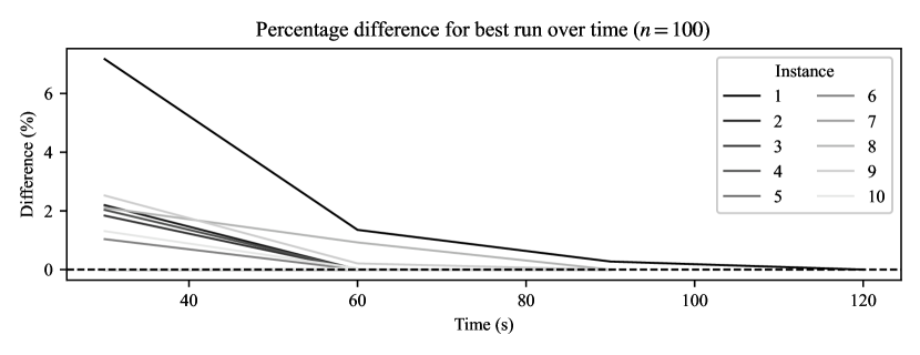
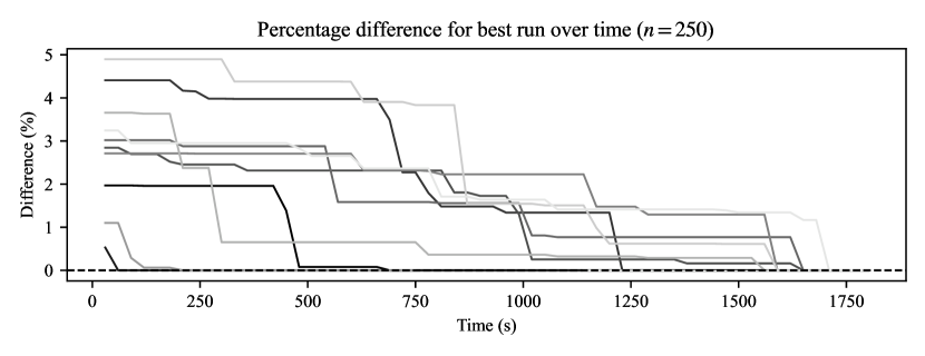
Figure 11: Average percentage difference over time for instances with $n=100$ and $n=250$ customers (tracking solutions after 30 seconds)

Comparison with the integer L-shaped method of Vásquez et al. [2021]

Table 5 shows the comparison with the integer L-shaped method of Vásquez et al. [2021]. The authors provided us with their result data using a maximum run time of one hour. For the integer L-shaped method, Column “# Optimal” reports the number of instances solved to optimality. For the MD-SPP-H, we report the results achieved by MD-SPP-H for the best of the ten runs. Column “# Optimal” reports the number of instances where MD-SPP-H finds the same optimal value as the integer L-shaped method; and Column “# Worse” (resp., # Better) details the number of solutions where MD-SPP-H achieves a worse (resp., better) solution than the integer L-shaped method. Further, considering those instances where the integer L-shaped method does not prove optimality, Column “# Equal” shows the number of solutions for which the integer L-shaped method and MD-SPP-H find the same value. Column “Opt. gap (%)” is the average optimality gap reached by MD-SPP-H over all instances solved to optimality by the integer L-shaped method; Column “Diff (%)” shows the average percentage difference between the best-known value achieved by the integer L-shaped method (i.e., the upper bound given by the solver) and the value of MD-SPP-H over those instances not solved to optimality by the integer L-shaped method (a negative value indicates that MD-SPP-H outperforms the integer L-shaped method); and Column “Run time (s)” details the average run time (over 10 instances) needed by MD-SPP-H.

For instances with up to 17 customers, for which the integer L-shaped method finds the optimal solution for all instances, Table 5 shows that the MD-SPP-H reaches the optimal solution for most of the instances in a very short run time of less than 0.2 seconds. The optimality gap over those instances is below or equal to 0.4%. For instances with 18 and up to 20 customers, MD-SPP-H performs worse only for 3 out of 30 instances. For most instances, MD-SPP-H reaches the same solution value as the integer L-shaped method or even improves the solution. On average, MD-SPP-H improves the solution quality by 1.4% for instances that are not solved to optimality by the integer L-shaped method; see Column Diff (%).

Table 5: Comparison between MD-SPP-H and the integer L-shaped method of Vásquez et al. [2021].

Customers	Instances		L-shaped		MD-SPP-H
			# Optimal		# Optimal	# Worse	# Better	# Equal	Opt. gap (%)	Diff (%)	Run time (s)
10	10		10		8	2	0	0	0.10	-	0.04
11	10		10		7	3	0	0	0.40	-	0.05
12	10		10		7	3	0	0	0.23	-	0.06
13	10		10		9	1	0	0	0.33	-	0.09
14	10		10		9	1	0	0	0.05	-	0.10
15	10		10		8	2	0	0	0.18	-	0.12
16	10		10		9	1	0	0	0.12	-	0.15
17	10		10		10	0	0	0	0.00	-	0.18
18	10		6		4	2	2	2	0.25	-1.61	0.28
19	10		1		1	1	6	2	0.00	-1.08	0.37
20	10		1		1	0	8	1	0.00	-1.51	0.43
All	110		88		73	16	16	5	0.15	-1.40	0.17

Appendix Online Appendix A Comparison with solution approaches for the FSTSP-MD

Run times of MD-SPP and IGH

Figure 12 shows the actual run times needed by MD-SPP-H and IGH. Overall, results show that both MD-SPP-H and IGH require less than 600 seconds for instances up to 75 customers. This is because Gonzalez-R et al. [2020] also consider as termination criterion a maximum number of 50 consecutive iterations without improvement. Although there is a slight increase in reported run times for scenarios with smaller speed ratios, we consistently report nearly identical run times for instances with higher speed ratios.

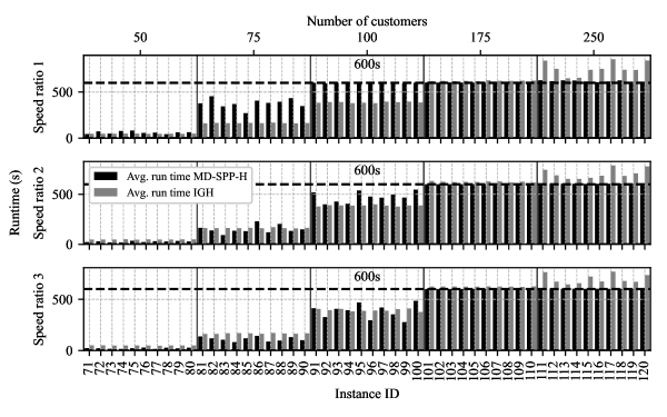
Figure 12: Average run times of MD-SPP-H and IGH (based on results published by Gonzalez-R et al. [2020]), considering $50,75,100,175$ and $250$ uniformly distributed customers.

Comparison with IGH over single- and double-center instances

Figures 13 and 14 report the relative percentage differences achieved by MD-SPP-H over the IGH heuristic of Gonzalez-R et al. [2020], considering the single- and double-center customer distributions and at least 50 customers. We observe similar, yet slightly reduced improvements for the two non-uniform distributions compared to the uniform distribution.

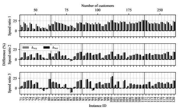
Figure 13: Percentage difference between MD-SPP and IGH (based on solutions published by Gonzalez-R et al. [2020]), considering $50,75,100,175$ and $250$ with a single-center customer distribution.

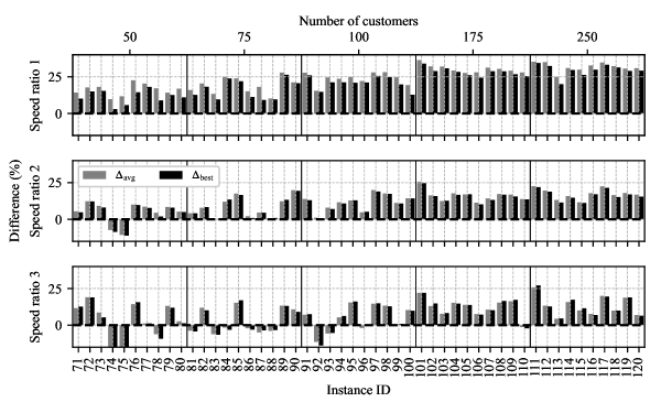
Figure 14: Percentage difference between MD-SPP and IGH (based on solutions published by Gonzalez-R et al. [2020]), considering $50,75,100,175$ and $250$ with a double-center customer distribution.

Appendix Online Appendix B Comparison with solution approaches for the FSTSP

Comparison with EP-All over single- and double-center instances

Figures 15 and 16 report the relative percentage differences achieved by MD-SPP-H over the EP-All heuristic of Agatz et al. [2018], considering the single- and double-center customer distributions and at least 50 customers. Averaged over all 50 instances with single-center customer distribution, MD-SPP-H improves the best-found solution value by $\Delta_{\text{best}}$ = 3.9%. The average solution value reached by MD-SPP-H improves the solution found by EP-All by $\Delta_{\text{avg}}$= 2.2% (average over the 50 instances). In the double-center cases, we report average improvements of the best-found solution value and average solution value reached by MD-SPP-H of $\Delta_{\text{best}}$ = 3.6% and $\Delta_{\text{avg}}$= 2.1%, respectively. These improvements are modestly lower than those noted for uniform customer distributions.

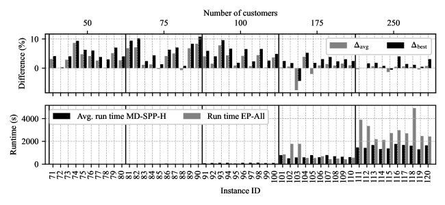
Figure 15: Benchmark of MD-SPP-H with solution published by Agatz et al. [2018]: single-center distribution and at least 50 customers.

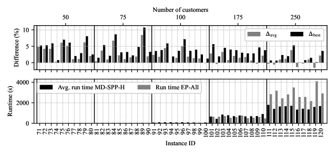
Figure 16: Benchmark of MD-SPP-H with solution published by Agatz et al. [2018]: double-center distribution and at least 50 customers.

Comparison with SPP-All over single- and double-center instances

Figures 17 and 18 report the relative percentage differences achieved by MD-SPP-H over the SPP-All heuristic of Kundu et al. [2021], considering the single- and double-center customer distributions and at least 50 customers. On average, over the 50 instances with single-center customer distribution, we report improvements of $\Delta_{\text{best}}$ = 2.7% and $\Delta_{\text{avg}}$= 0.9% for the best-found and average solution value, respectively. The corresponding values for the double-center instances are $\Delta_{\text{best}}$ = 3.1% and $\Delta_{\text{avg}}$= 1.5%.

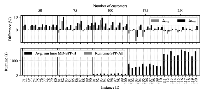
Figure 17: Benchmark of MD-SPP-H with solution published by Kundu et al. [2021]: single-center distribution and at least 50 customers.

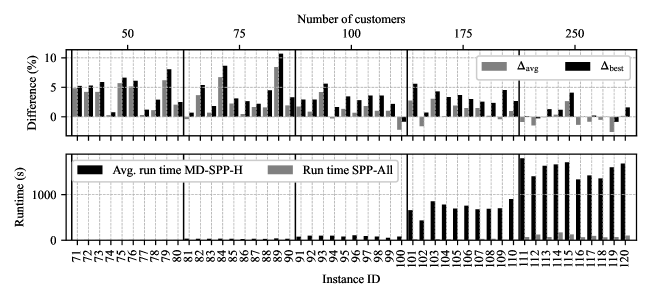
Figure 18: Benchmark of MD-SPP-H with solution published by Kundu et al. [2021]: double-center distribution and at least 50 customers.

Appendix Online Appendix C Impact of Individual Parameters and Their Interaction on Time Savings and Delivery System Performance

In the following, we present the supplementary results of the full factorial experiment we conducted to gain managerial insights into the collaborative truck-and-drone delivery system. The results are sorted based on the customer distribution: uniform, single- and double-center. If not included in the main manuscript, we present plots summarizing the observed percentage time savings, the maximum drone flight duration of a single flight, and the total drone flight duration. We average the results over ten instances for each scenario.

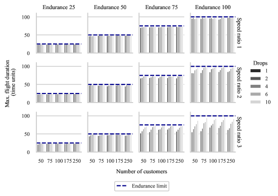
Figure 21: Comparison of average observed maximum drone flight duration over ten instances and imposed drone flight endurance limit for instances with single-center customer distribution

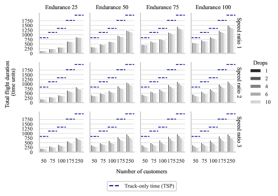
Figure 22: Comparison of average observed total drone flight duration (i.e., sum over all drone flights) over ten instances and truck-only delivery system completion time for instances with single-center customer distribution

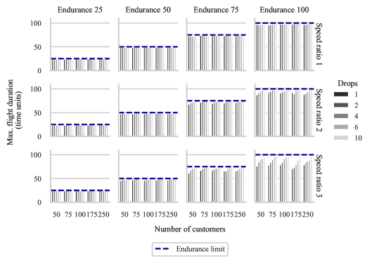
Figure 24: Comparison of average observed maximum drone flight duration over ten instances and imposed drone flight endurance limit for instances with double-center customer distribution

References

- Agatz et al. [2018] Agatz, N., Bouman, P., & Schmidt, M. (2018). Optimization approaches for the traveling salesman problem with drone. Transportation Science, 52, 739–1034. doi:10.1287/trsc.2017.0791.
- Alamalhodaei [2021] Alamalhodaei, A. (2021). Wingcopter debuts a triple-drop drone to create ‘logistical highways in the sky’. URL: https://techcrunch.com/2021/04/27/wingcopter-debuts-a-triple-drop-drone-to-create-logistical-highways-in-the-sky/.
- Applegate et al. [2006] Applegate, D. L., Bixby, R. E., Chvatál, V., & Cook, W. J. (2006). The traveling salesman problem: A computational study. Princeton, US: Princeton University Press.
- Chauhan et al. [2019] Chauhan, D., Unnikrishnan, A., & Figliozzi, M. (2019). Maximum coverage capacitated facility location problem with range constrained drones. Transportation Research Part C: Emerging Technologies, 99, 1–18.
- Chen [2023] Chen, C. (2023). Amazon reveals first photos of the new Prime Air delivery drone. URL: https://www.aboutamazon.com/news/transportation/amazon-prime-air-drone-delivery-mk30-photos.
- Chung et al. [2020] Chung, S. H., Sah, B., & Lee, J. (2020). Optimization for drone and drone-truck combined operations: A review of the state of the art and future directions. Computers and Operations Research, 123, 105004.
- Cornell et al. [2023] Cornell, A., Mahan, S., & Riedel, R. (2023). Commercial drone deliveries are demonstrating continued momentum in 2023. URL: https://www.mckinsey.com/industries/aerospace-and-defense/our-insights/future-air-mobility-blog/commercial-drone-deliveries-are-demonstrating-continued-momentum-in-2023.
- Dayarian et al. [2020] Dayarian, I., Savelsbergh, M., & Clarke, J.-P. (2020). Same-day delivery with drone resupply. Transportation Science, 54, 229–249.
- Dukkanci et al. [2023] Dukkanci, O., Campbell, J. F., & Kara, B. Y. (2023). Facility location decisions for drone delivery: A literature review. European Journal of Operational Research, In Press. doi:10.1016/j.ejor.2023.10.036.
- Etherington [2017] Etherington, D. (2017). Mercedes-Benz kicks off drone delivery pilot in Zurich. URL: https://techcrunch.com/2017/09/28/mercedes-benz-kicks-off-drone-delivery-pilot-in-zurich/.
- Gonzalez-R et al. [2020] Gonzalez-R, P. L., Canca, D., Andrade-Pineda, J. L., Calle, M., & Leon-Blanco, J. M. (2020). Truck-drone team logistics: A heuristic approach to multi-drop route planning. Transportation Research Part C: Emerging Technologies, 114, 657–680. doi:10.1016/j.trc.2020.02.030.
- Gu et al. [2022] Gu, R., Poon, M., Luo, Z., Liu, Y., & Liu, Z. (2022). A hierarchical solution evaluation method and a hybrid algorithm for the vehicle routing problem with drones and multiple visits. Transportation Research Part C: Emerging Technologies, 141. doi:10.1016/j.trc.2022.103733.
- Ha et al. [2018] Ha, Q. M., Deville, Y., Pham, Q. D., & Hà, M. H. (2018). On the min-cost traveling salesman problem with drone. Transportation Research Part C: Emerging Technologies, 86, 597–621. doi:10.1016/j.trc.2017.11.015.
- Holland et al. [2017] Holland, C., Levis, J., Nuggehalli, R., Santilli, B., & Winters, J. (2017). UPS optimizes delivery routes. Interfaces, 47, 8–23. doi:10.1287/INTE.2016.0875.
- Jeong et al. [2019] Jeong, H. Y., Song, B. D., & Lee, S. (2019). Truck-drone hybrid delivery routing: Payload-energy dependency and No-Fly zones. International Journal of Production Economics, 214, 220–233. doi:10.1016/j.ijpe.2019.01.010.
- Jiang et al. [2024] Jiang, J., Dai, Y., Yang, F., & Ma, Z. (2024). A multi-visit flexible-docking vehicle routing problem with drones for simultaneous pickup and delivery services. European Journal of Operational Research, 312, 125–137. doi:10.1016/j.ejor.2023.06.021.
- Kitjacharoenchai et al. [2019] Kitjacharoenchai, P., Ventresca, M., Moshref-Javadi, M., Lee, S., Tanchoco, J. M., & Brunese, P. A. (2019). Multiple traveling salesman problem with drones: Mathematical model and heuristic approach. Computers and Industrial Engineering, 129, 14–30. doi:10.1016/j.cie.2019.01.020.
- Kundu et al. [2021] Kundu, A., Escobar, R. G., & Matis, T. I. (2021). An efficient routing heuristic for a drone-assisted delivery problem. IMA Journal of Management Mathematics, 33, 583–601. doi:10.1093/imaman/dpab039.
- Kundu et al. [2020] Kundu, A., Gatica, R., & Matis, T. I. (2020). Results for the Implementation of EP-All and SPP-All heuristic. doi:10.5281/zenodo.4007382.
- Leon-Blanco et al. [2022] Leon-Blanco, J. M., Gonzalez-R, P. L., Andrade-Pineda, J. L., Canca, D., & Calle, M. (2022). A multi-agent approach to the truck multi-drone routing problem. Expert Systems with Applications, 195, 116604. doi:10.1016/j.eswa.2022.116604.
- Liu et al. [2021] Liu, Y., Liu, Z., Shi, J., Wu, G., & Pedrycz, W. (2021). Two-echelon routing problem for parcel delivery by cooperated truck and drone. IEEE Transactions on Systems, Man, and Cybernetics: Systems, 51, 7450–7465. doi:10.1109/TSMC.2020.2968839.
- Luo et al. [2022] Luo, Z., Gu, R., Poon, M., Liu, Z., & Lim, A. (2022). A last-mile drone-assisted one-to-one pickup and delivery problem with multi-visit drone trips. Computers and Operations Research, 148, 106015. doi:10.1016/j.cor.2022.106015.
- Luo et al. [2021] Luo, Z., Poon, M., Zhang, Z., Liu, Z., & Lim, A. (2021). The multi-visit traveling salesman problem with multi-drones. Transportation Research Part C: Emerging Technologies, 128, 103172. doi:10.1016/j.trc.2021.103172.
- Macrina et al. [2020] Macrina, G., Pugliese, L. D. P., Guerriero, F., & Laporte, G. (2020). Drone-aided routing: A literature review. Transportation Research Part C: Emerging Technologies, 120, 102762.
- Meng et al. [2024] Meng, S., Chen, Y., & Li, D. (2024). The multi-visit drone-assisted pickup and delivery problem with time windows. European Journal of Operational Research, 314, 685–702. doi:10.1016/j.ejor.2023.10.021.
- Moshref-Javadi & Winkenbach [2021] Moshref-Javadi, M., & Winkenbach, M. (2021). Applications and research avenues for drone-based models in logistics: A classification and review. Expert Systems with Applications, 177, 114854.
- Murray & Chu [2015] Murray, C. C., & Chu, A. G. (2015). The flying sidekick traveling salesman problem: Optimization of drone-assisted parcel delivery. Transportation Research Part C: Emerging Technologies, 54, 86–109. doi:10.1016/j.trc.2015.03.005.
- Pina-Pardo et al. [2021] Pina-Pardo, J. C., Silva, D. F., & Smith, A. E. (2021). The Traveling Salesman Problem with Release Dates and Drone Resupply. Computers and Operations Research, 129, 105170.
- Pina-Pardo et al. [2024] Pina-Pardo, J. C., Silva, D. F., Smith, A. E., & Gatica, R. A. (2024). Fleet resupply by drones for last-mile delivery. European Journal of Operational Research16, 316, 168–182. doi:10.1016/j.ejor.2024.01.045.
- Poikonen & Golden [2020] Poikonen, S., & Golden, B. (2020). Multi-visit drone routing problem. Computers and Operations Research, 113, 104802. doi:10.1016/j.cor.2019.104802.
- Prins et al. [2014] Prins, C., Lacomme, P., & Prodhon, C. (2014). Order-first split-second methods for vehicle routing problems: A review. Transportation Research Part C: Emerging Technologies, 40, 179–200. doi:10.1016/j.trc.2014.01.011.
- Raj & Murray [2020] Raj, R., & Murray, C. (2020). The multiple flying sidekicks traveling salesman problem with variable drone speeds. Transportation Research Part C: Emerging Technologies, 120, 102813. doi:10.1016/j.trc.2020.102813.
- Roberti & Ruthmair [2021] Roberti, R., & Ruthmair, M. (2021). Exact methods for the traveling salesman problem with drone. Transportation Science, 55, 315–335. doi:10.1287/TRSC.2020.1017.
- Sakharkar [2021] Sakharkar, A. (2021). A2Z Drone Delivery unveils a multi-drop dual-payload delivery drone. URL: https://www.inceptivemind.com/a2z-drone-delivery-rdsx-multi-drop-dual-payload-delivery-drone/20842/.
- Samet [2023] Samet, A. (2023). Ecommerce growth worldwide will pick up before tapering off. URL: https://www.insiderintelligence.com/content/ecommerce-growth-worldwide-will-pick-up-before-tapering-off.
- Savelsbergh [1992] Savelsbergh, M. W. P. (1992). The vehicle routing problem with time windows: Minimizing route duration. ORSA Journal on Computing, 4, 146–154.
- Schermer et al. [2019a] Schermer, D., Moeini, M., & Wendt, O. (2019a). A hybrid VNS/Tabu search algorithm for solving the vehicle routing problem with drones and en route operations. Computers and Operations Research, 109, 134–158. doi:10.1016/j.cor.2019.04.021.
- Schermer et al. [2019b] Schermer, D., Moeini, M., & Wendt, O. (2019b). A matheuristic for the vehicle routing problem with drones and its variants. Transportation Research Part C: Emerging Technologies, 106, 166–204.
- Statista [2023] Statista (2023). Global last mile delivery market size 2020-2027. URL: https://www.statista.com/statistics/1286612/last-mile-delivery-market-size-worldwide/.
- Supply Chain Dive [2023] Supply Chain Dive (2023). Consumers want ultrafast delivery — and they want it today. URL: https://www.supplychaindive.com/spons/consumers-want-ultrafast-delivery-and-they-want-it-today/646011/.
- Vasani [2023] Vasani, S. (2023). FAA clears UPS delivery drones for longer-range flights. URL: https://www.theverge.com/2023/9/6/23861764/faa-ups-delivery-drones-amazon-prime-air.
- Vásquez et al. [2021] Vásquez, S. A., Angulo, G., & Klapp, M. A. (2021). An exact solution method for the TSP with Drone based on decomposition. Computers and Operations Research, 127, 105127. doi:10.1016/j.cor.2020.105127.
- Wang & Sheu [2019] Wang, Z., & Sheu, J. B. (2019). Vehicle routing problem with drones. Transportation Research Part B: Methodological, 122, 350–364. doi:10.1016/j.trb.2019.03.005.
- Windras Mara et al. [2022] Windras Mara, S. T., Rifai, A. P., & Sopha, B. M. (2022). An adaptive large neighborhood search heuristic for the flying sidekick traveling salesman problem with multiple drops. Expert Systems with Applications, 205, 117647. doi:10.1016/j.eswa.2022.117647.
- Wingcopter [2023] Wingcopter (2023). Wingcopter 198. URL: https://wingcopter.com/wingcopter-198.
- Yin et al. [2023] Yin, Y., Li, D., Wang, D., Ignatius, J., Cheng, T. C., & Wang, S. (2023). A branch-and-price-and-cut algorithm for the truck-based drone delivery routing problem with time windows. European Journal of Operational Research, 309, 1125–1144. doi:10.1016/j.ejor.2023.02.030.
- Zhu et al. [2022] Zhu, T., Boyles, S. D., & Unnikrishnan, A. (2022). Two-stage robust facility location problem with drones. Transportation Research Part C: Emerging Technologies, 137, 103563. doi:10.1016/J.TRC.2022.103563.