Discretize first, filter next: learning divergence-consistent closure models for large-eddy simulation

Abstract

We propose a new neural network based large eddy simulation framework for the incompressible Navier-Stokes equations based on the paradigm “discretize first, filter and close next”. This leads to full model-data consistency and allows for employing neural closure models in the same environment as where they have been trained. Since the LES discretization error is included in the learning process, the closure models can learn to account for the discretization.

Furthermore, we introduce a new divergence-consistent discrete filter defined through face-averaging. The new filter preserves the discrete divergence-free constraint by construction, unlike general discrete filters such as volume-averaging filters. We show that using a divergence-consistent LES formulation coupled with a convolutional neural closure model produces stable and accurate results for both a-priori and a-posteriori training, while a general (divergence-inconsistent) LES model requires a-posteriori training or other stability-enforcing measures.

[cwi] organization=Scientific Computing Group, Centrum Wiskunde & Informatica, addressline=Science Park 123, city=Amsterdam, postcode=1098 XG, country=The Netherlands [eindhoven] organization=Centre for Analysis, Scientific Computing and Applications, Eindhoven University of Technology, addressline=PO Box 513, city=Eindhoven, postcode=5600 MB, country=The Netherlands

1 Introduction

The incompressible Navier-Stokes equations form a model for the movement of fluids. They can be solved numerically on a grid using discretization techniques such as finite differences [28], finite volumes, or pseudo-spectral methods [50, 55]. The important dimensionless parameter in the incompressible Navier-Stokes equations is the Reynolds number $\mathrm{Re}=\frac{UL}{\nu}$, where $L$ is a characteristic length scale, $U$ is a characteristic velocity, and $\nu$ the kinematic viscosity. For high Reynolds numbers, the flow becomes turbulent. Resolving all the scales of motion of turbulent flows requires highly refined computational grids. This is computationally expensive [54, 57, 56, 72].

Large eddy simulation (LES) aims to resolve only the large scale features of the flow, as opposed to direct numerical simulation (DNS), where all the scales are resolved [54, 8]. The large scales of the flow, here denoted $\bar{u}$, are extracted from the full solution $u$ using a spatial filter. The equations for the large scales are then obtained by filtering the Navier-Stokes equations. The large scale equations (filtered DNS equations) are not closed, as they still contain terms depending on the small scales. It is common to group the contributions of the unresolved scales into a single commutator error term, that we denote $c(u,\bar{u})$. Large eddy simulation requires modeling this term as a function of the large scales only. The common approach is to introduce a closure model $m(\bar{u},\theta)\approx c(u,\bar{u})$ to remove the small scale dependency [54, 57, 8], where $\theta$ are problem-specific model parameters. The closure model accounts for the effect of the sub-filter scales on the resolved scales. Traditional closure models account for the energy lost to the sub-filter eddies. A simple approach to account for this energy transfer is to add an additional diffusive term to the LES equations. These closure models are known as eddy viscosity models. This includes the well known standard Smagorinsky model [66, 37, 38].

The filter can be either be known explicitly or implicitly. In the latter case, the (coarse) discretization itself is acting as a filter. Note that the distinction explicit versus implicit is not always clear, as an explicitly defined filter can still be linked to the discretization. Sometimes the filter is only considered to be explicit when the filter width is fully independent from the LES discretization size [6]. The type of filtering employed results in a distinction between explicit and implicit LES. Explicit LES [43, 20, 21] refers to a technique where the filter is explicitly used inside the convection term of the LES equations (as opposed to applying the filter in the exact filtered DNS evolution equations, where the filter is applied by definition). The LES solution (that we denote by $\bar{v}$) already represents a filtered quantity, namely the filtered DNS solution $\bar{u}$. Applying the filter again inside the LES equations can thus be seen as computing a quantity that is filtered twice. The main advantage is stability [7] and to prevent the growth of high-wavenumber components [43, 20]. Note that this technique requires explicit access to the underlying filter. Implicit LES is used to describe the procedure where the DNS equations are used in their original form, and the closure model is added as a correction (regardless of whether the filter is known explicitly or not). Here, the filter itself is not required to evaluate the LES equations, but knowledge of certain filter properties such as the filter width is used to choose the closure model. In the standard Smagorinsky model for example, the filter width is used as a model parameter. If the exact filter is not known, this parameter is typically chosen to be proportional to the grid spacing.

Recently, machine learning has been used to learn closure models, focusing mostly on implicit LES [4, 5, 6, 19, 29, 36, 35, 41, 47, 65, 63, 64]. The idea is to represent the closure model $m(\bar{u},\theta)$ by an artificial neural network (ANN). ANNs are in principle a good candidate as they are universal function approximators [3, 13]. However, using ANNs as closure models typically suffers from stability issues, which have been attributed to a so-called model-data inconsistency: the environment in which the neural network is trained is not the same in which it is being used [6]. Several approaches like backscatter clipping, a-posteriori training and projection onto an eddy-viscosity basis have been used to enforce stability [52, 41, 4] – for an overview, see [60]. Our view is that one of the problems that lies at the root of the model-data inconsistency is a discrepancy between the LES equations (obtained by first filtering the continuous Navier-Stokes equations, then discretizing) and the training data (obtained by discretizing the Navier-Stokes equations, and then applying a discrete filter).

Figure 1: Proposed route (in green) to a discrete LES model, based on“discretize first, then filter” instead of “filter first, then discretize” (in red).

Our key insight is that the LES equations can also be obtained by “discretizing first” instead of “filtering first”: following the green instead of the red route in figure 1. In other words, by discretizing the PDE first, and then applying a discrete filter, the model-data inconsistency issue can be avoided and one can generate exact training data for the discrete LES equations. Training data obtained by filtering discrete DNS solutions is fully consistent with the environment where the discrete closure model is used. The resulting LES equations do not have a coarse grid discretization error, but an underlying fine grid discretization error and a commutator error from the discrete filter, which can be learned using a neural network. In our recent work [1], we showed the benefits of the “discretize first” approach on a 1D convection equation. With the discretize-first approach we obtain stable results without the need for the stabilizing techniques mentioned above (backscatter clipping, a-posteriori training, projection onto an eddy-viscosity basis).

In the current paper, the goal is to extend the “discretize first” approach to the full 3D incompressible Navier-Stokes equations. One major challenge that appears in incompressible Navier-Stokes is the presence of the divergence-free constraint. We show that discrete filters are in general not divergence-consistent (meaning that divergence-free DNS solutions do not stay divergence-free upon filtering) and we propose a novel divergence-consistent discrete filter. Overall, the main result is that our divergence-consistent neural closure models lead to stable simulations.

In addition, we remark that divergence-consistent filtering is an important step towards LES closure models that satisfy an energy inequality. Such models were developed by us in [70] for one-dimensional equations with quadratic nonlinearity (Burgers, Korteweg - de Vries). When extending this approach to 3D LES, the derivation of the energy inequality hinges on having a divergence-free constraint on the filtered solution field.

Our article is structured as follows. In section 2, we present the discrete DNS equations that serve as the ground truth in our problem, based on a second order accurate finite volume discretization on a staggered grid. In section 3, we introduce discrete filtering. Unclosed equations for the large scales are obtained. We show that the filtered velocity is not automatically divergence-free. We then present a novel divergence preserving discrete filter on the staggered grid. In section 4, we present our discrete closure modeling framework, resulting in two discrete LES formulations. We discuss the validity of the LES models in terms of divergence-consistency. A discussion follows on the choice of closure model and how we can learn the closure model parameters. In section 5, we present the results of numerical experiments on a decaying turbulence test case. Section 6 ends with concluding remarks.

2 Direct numerical simulation of all scales

In this section, we present the continuous Navier-Stokes equations and define a discretization aimed at resolving all the scales of motion. The resulting discrete equations will serve as the ground truth for learning an equation for the large scales.

2.1 The Navier-Stokes equations

The incompressible Navier-Stokes equations describe conservation of mass and conservation of momentum, which can be written as a divergence-free constraint and an evolution equation:

$$\nabla\cdot u =0,$$ (1)

$$\frac{\partial u}{\partial t}+\nabla\cdot(uu^{\mathsf{T}}) =-\nabla p+\nu\nabla^{2}u+f,$$ (2)

where $\Omega\subset\mathbb{R}^{d}$ is the domain, $d\in\{2,3\}$ is the spatial dimension, $u=(u^{1},\dots,u^{d})$ is the velocity field, $p$ is the pressure, $\nu$ is the kinematic viscosity, and $f=(f^{1},\dots,f^{d})$ is the body force per unit of volume. The velocity, pressure, and body force are functions of the spatial coordinate $x=(x^{1},\dots,x^{d})$ and time $t$. For the remainder of this work, we assume that $\Omega$ is a rectangular domain with periodic boundaries, and that $f$ is constant in time.

2.2 Spatial discretization

For the discretization scheme, we use a staggered Cartesian grid as proposed by Harlow and Welch [28]. Staggered grids have excellent conservation properties [39, 53], and in particular their exact discrete divergence-free constraint is important for this work. Details about the discretization can be found in A.

Figure 2: Finite volume discretization on a staggered grid. The pressure is defined in the volume center, and the velocity components on the volume faces.

We partition the domain $\Omega$ into $N$ finite volumes. Let $u(t)\in\mathbb{R}^{dN}$ and $p(t)\in\mathbb{R}^{N}$ be vectors containing the unknown velocity and pressure components in their canonical positions as shown in figure 2. They are not to be confused with their space-continuous counterparts $u(x,t)$ and $p(x,t)$, which will no longer be referred to in what follows. The discrete and continuous versions of $u$ and $p$ have the same physical dimensions.

Equations (1) and (2) are discretized as

$$Du =0,$$ (3)

$$\frac{\mathrm{d}u}{\mathrm{d}t} =F(u)-Gp,$$ (4)

where $D\in\mathbb{R}^{N\times dN}$ is the divergence operator, $G=-\Omega_{u}^{-1}D^{\mathsf{T}}\Omega_{p}\in\mathbb{R}^{dN\times N}$ is the gradient operator, $\Omega_{u}\in\mathbb{R}^{dN\times dN}$ and $\Omega_{p}\in\mathbb{R}^{N\times N}$ are element-wise scaling operators containing the velocity and pressure volume sizes, and $F(u)\in\mathbb{R}^{dN}$ contains the convective, diffusive, and body force terms.

2.3 Pressure projection

The two vector equations (3) and (4) form an index-2 differential-algebraic equation system [26, 27], consisting of a divergence-free constraint and an evolution equation. Given $u$, the pressure can be obtained by solving the discrete Poisson equation $0=DF(u)-DGp$, which is obtained by differentiating the divergence-free constraint in time. This can also be written

$$Lp=\Omega_{p}DF(u),$$ (5)

where the Laplace matrix $L=\Omega_{p}DG=-\Omega_{p}D\Omega_{u}^{-1}D^{\mathsf{T}}\Omega_{p}$ is symmetric and negative semi-definite. We denote by $L^{\dagger}$ the solver to the scaled pressure Poisson equation (5). Since no boundary value for the pressure is prescribed, $L$ is rank-$1$ deficient and the pressure is only determined up to a constant. We set this constant to zero by choosing

$$L^{\dagger}=\begin{pmatrix}I&0\end{pmatrix}\begin{pmatrix}L&e\\ e^{\mathsf{T}}&0\end{pmatrix}^{-1}\begin{pmatrix}I\\ 0\end{pmatrix},$$ (6)

where $e=(1,\dots,1)\in\mathbb{R}^{N}$ is a vector of ones and the additional degree of freedom enforces the constraint of an average pressure of zero (i.e. $e^{\mathsf{T}}L^{\dagger}=0$) [42]. In this case we still have $LL^{\dagger}=I$, even though $L^{\dagger}L\neq I$.

We now introduce the projection operator $P$, which plays an important role in the development of our new closure model strategy in section 3: $P=I-GL^{\dagger}\Omega_{p}D$. It is used to make velocity fields divergence-free [15], since $DP=D-\Omega_{p}^{-1}LL^{\dagger}\Omega_{p}D=0$. It naturally follows that $P$ is a projector, since $P^{2}=P-GL^{\dagger}\Omega_{p}DP=P$.

Having defined $P$, it is (at least formally) possible to eliminate the pressure from equations (3)-(4) into a single “pressure-free” evolution equation for the velocity [59], given by

$$\frac{\mathrm{d}u}{\mathrm{d}t}=PF(u).$$ (7)

This way, an initially divergence-free velocity field $u$ stays divergence-free regardless of what forcing term $F$ is applied. We note that equation (7) alone does not enforce the divergence-free constraint, as it also requires the initial conditions to be divergence-free.

$L^{\dagger}$ and $P$ are non-local operators that are not explicitly assembled, but their action on vector fields is computed on demand using an appropriate linear solver. Formulation (7) is used as a starting point for developing a new filtering technique in section 3.

2.4 Time discretization

We use a standard fourth order accurate Runge-Kutta method (RK4) for the incompressible Navier-Stokes equations [59]. While explicit methods may require smaller time steps (depending on the problem-specific trade-off of stability versus accuracy), they are easier to differentiate with automatic differentiation tools.

Given the solution $u_{n}$ at a time $t_{n}$, the next solution at a time $t_{n+1}$ is given by

$$u_{n+1}=u_{n}+\Delta t_{n}\sum_{i=1}^{s}b_{i}k_{i},$$ (8)

where

$$k_{i}=PF\left(u_{n}+\Delta t_{n}\sum_{j=1}^{i-1}a_{ij}k_{j}\right),$$ (9)

$\Delta t_{n}=t_{n+1}-t_{n}$, $s$ is the number of stages, $a\in\mathbb{R}^{s\times s}$, and $b\in\mathbb{R}^{s}$. In practice, each of the RK steps (9) are performed by first computing a tentative (non-divergence-free) velocity field, subsequently solving a pressure Poisson equation, and then correcting the velocity field to be divergence-free. As the method is explicit, this is equivalent to (9) and does not introduce a splitting error [59]. For RK4, we set $s=4$, $b_{1}=1/6$, $b_{2}=1/3$, $b_{3}=1/3$, $b_{4}=1/6$, $a_{21}=1/2$, $a_{32}=1/2$, $a_{43}=1$, and the other coefficients $a_{ij}=0$.

3 Discrete filtering and divergence-consistency

The DNS discretization presented in the previous section is in general too expensive to simulate for problems of practical interest, and it is only used to generate reference data for a limited number of test cases. In this section, we present discrete filtering from the fine DNS grid to a coarse grid in order to alleviate the computational burden. This means we filter the discretized equations, in contrast to many existing approaches, which filter the continuous Navier-Stokes equations, and then apply a discretization. The advantages of “discretizing first” were already mentioned in section 1. However, one disadvantage of “discretizing first” is that the filtered velocity field is in general not divergence free. We present a new face-averaging filter that preserves the divergence-free constraint for the filtered velocity.

3.1 Filtering from fine to coarse grids

We consider two computational grids: a fine grid of size $N\in\mathbb{N}^{d}$ and a coarse grid of size $\bar{N}\in\mathbb{N}^{d}$, with $\bar{N}_{\alpha}\leq N_{\alpha}$ for all $\alpha\in\{1,\dots,d\}$. The operators $D$, $F$, $G$, $P$, etc., are defined on the fine grid. On the coarse grid, similar operators are denoted $\bar{D}$, $\bar{F}$, $\bar{G}$, $\bar{P}$, etc.

Consider a flow problem. We assume that the flow is fully resolved on the fine grid, meaning that the grid spacing is at least twice as small as the smallest significant spatial structure of the flow. The resulting fully resolved solution $u\in\mathbb{R}^{dN}$ is referred to as the DNS solution. In addition, we assume that the flow is not fully resolved on the coarse grid, meaning that the coarse grid spacing is larger than the smallest significant spatial structure of the flow. The aim is to solve for the large scale features of $u$ on the coarse grid. For this purpose, we construct a discrete spatial filter $\Phi\in\mathbb{R}^{d\bar{N}\times dN}$. The resulting filtered DNS velocity field is given by

$$\bar{u}=\Phi u\in\mathbb{R}^{d\bar{N}},$$ (10)

and is a coarse-grid quantity. We stress that $\bar{u}$ is by definition a consequence of the DNS. It is not obtained by solving the Navier-Stokes equations on the coarse grid. That is instead the goal in the next sections.

Since $\Phi$ is a coarse-graining filter, it does not generally commute with discrete differential operators. In particular, the divergence-free constraint is preserved for continuous convolutional filters, but this is not automatically the case for discrete filters. We consider this property in detail, and investigate its impact on the resulting large scale equations.

3.2 Equation for large scales

When directly filtering the differential-algebraic system (3)-(4), multiple challenges arise. These are detailed in C and summarized here:

• The filter $\Phi$ works on inputs defined in the velocity points, and is targeted at filtering the momentum equation. It is not directly clear how to filter the divergence-free constraint (which is defined in the pressure points), and whether a second filter needs to be defined for the pressure points.

• The momentum equation includes a pressure term. While its gradient can be filtered with $\Phi$, it is not clear what a filtered pressure $\bar{p}$ should be, or how it should appear in the filtered momentum equation.

To circumvent these issues, we propose to differentiate the discrete divergence constraint first (to remove the pressure), and then apply the filter to the pressure-free DNS equation (7). This results in the sequence “discretize – differentiate constraint – filter”, as shown by solid green arrows in figure 3. The advantage over the route defined by dashed green arrows, “discretize – filter”, is that we do not need to consider the pressure or the divergence-free constraint, and a single filter for the velocity field is sufficient. The “implied” filtered pressure will be discussed in section 4.1. The resulting equation for the filtered DNS-velocity $\bar{u}$ is $\frac{\mathrm{d}\bar{u}}{\mathrm{d}t}=\Phi PF(u)$, which is rewritten as

$$\frac{\mathrm{d}\bar{u}}{\mathrm{d}t}=\bar{P}\bar{F}(\bar{u})+c(u,\bar{u}),$$ (11)

with the unclosed commutator error defined by

$$c(u,\bar{u})=\Phi PF(u)-\bar{P}\bar{F}(\bar{u}).$$ (12)

A crucial point is that when filtering from a fine grid to a coarse grid, one generally does not get a divergence-free filtered velocity field ($\bar{D}\bar{u}\neq 0$), as discrete filtering and discrete differentiation do not generally commute.

Figure 3: Alternative view of figure 1 to highlight the effect of differentiating the constraint. The red arrows show the traditional route of filtering first and then discretizing. The solid green arrows show our proposed route of discretizing first, then differentiating the constraint, then filtering, and finally reintroducing a pressure term (if the filter is divergence-consistent). This is done to circumvent the pressure problems of the dashed green route (discretizing first, then filtering).

3.3 New divergence-consistent discrete filter

Our novel approach is to design the filter and coarse grid such that the divergence-free constraint is preserved. This is achieved by merging fine DNS volumes to form coarse LES volumes, such that the faces of DNS and LES volumes overlap (as shown in figure 4). The extracted large scale velocities $\bar{u}=\Phi u$ are then obtained by averaging the DNS velocities that are found on the LES volume faces. We denote this face-averaging discrete filter by $\Phi^{\text{FA}}$. This approach to filtering also naturally generalizes to unstructured grids, as long as the coarse volume faces overlap with the fine ones. An example is shown to the right in figure 4 for triangular volumes.

Figure 4: Four coarse volumes (blue) and their fine grid sub-grid volumes (red) in 2D. For each of the coarse volume faces, the discrete filter $\Phi^{\text{FA}}$ combines the DNS velocities $u$ into one LES velocity $\bar{u}$ using averaging. The interior sub-grid velocities are not present in $\bar{u}$. The coarse grid pressure $\bar{p}$ is defined in the coarse volume centers, but is not obtained by filtering $p$. Instead, it is computed from $\bar{u}$. Left: Structured grid, used in this work. Right: Unstructured grid.

The face-averaging filter $\Phi^{\text{FA}}$ is different to more traditional volume-averaging filters such as the volume-averaging top-hat filter [57] (that we denote $\Phi^{\text{VA}}$). The face-averaging filter can be thought of as a top-hat filter acting on the dimensions orthogonal to the velocity components only, while the volume-averaging filter is averaging over all dimensions. In this work, we define the two discrete filters $\Phi^{\text{FA}}$ and $\Phi^{\text{VA}}$ with uniform weights and with filter width equal to the coarse grid spacing $\bar{\Delta}$. Since both filters are top-hat like, the filter width is defined as the diameter of the averaging domain in the infinity norm. Note that due to the normalization, all discrete velocity components $\bar{u}^{\alpha}_{J}$ and $u^{\alpha}_{I}$ share the same dimension as the continuous velocity $u^{\alpha}(x,t)$ (not velocity times area or velocity times volume).

The two discrete filter supports are compared in figure 5. One advantage of the face-averaging filter is that it does not require modifications at non-periodic boundaries, while the volume-averaging filter does (for example by using a volume of half the size and twice as large weights to avoid averaging outside solid walls). But the main advantage lies in the preservation of the divergence-free constraint, as we now show.

Figure 5: DNS velocity components $u$ contributing to a single filtered DNS component $\bar{u}$ for two filters. Both filters have a filter width equal to the grid size. Both $u(t)$ and $\bar{u}(t)$ share the same dimension as the continuous velocity $u(x,t)$. Left: Volume-averaging filter $\Phi^{\text{VA}}$. Right: Face-averaging filter $\Phi^{\text{FA}}$.

When $\bar{u}$ is obtained through face-averaging, the difference of fluxes entering and leaving an LES volume is equal to a telescoping sum of all sub-grid flux differences, which in turn is zero due to the fine grid divergence-free constraint. The proof is shown in B. Note that this property no longer holds if the weights are non-uniform or if the width is different from the coarse grid spacing. Our novel face-averaging filter thus preserves by construction the divergence-free constraint for the filtered DNS velocity:

$$\text{For}\ \Phi^{\text{FA}}:\ \boxed{\forall u,\ Du=0\implies\bar{D}\bar{u}=0.}$$ (13)

This property is the primary motivation for our filter choice (it can also be thought of as a discrete equivalent of the divergence theorem $\nabla\cdot u=0\implies\int_{\partial\mathcal{O}}u\cdot n\,\mathrm{d}\Gamma=0$ for all $\mathcal{O}$). It can be used to show that the face-averaging filter has the property

$$\bar{D}\Phi P=0$$ (14)

since, for all $u$, if $w=Pu$, then $Dw=0$ by definition of $P$, and thus $\bar{D}\Phi Pu=\bar{D}\Phi w=\bar{D}\bar{w}=0$ from (13). In other words, divergence-free fine grid velocity fields stay divergence-free upon filtering. For a general volume-averaging filter, we would not be able to guarantee that all the sub-grid fluxes cancel out, and we would not get a divergence-free constraint for $\bar{u}$. This constraint is often enforced anyways, possibly introducing unforeseen errors, as pointed out by Sirignano et al. [65]. With the face-averaging filter, we do not need to worry about such errors.

With our face-averaging filter choice, the momentum commutator error is divergence-free, since

$$\bar{D}c=\bar{D}\left(\frac{\mathrm{d}\bar{u}}{\mathrm{d}t}-\bar{P}\bar{F}(\bar{u})\right)=\frac{\mathrm{d}(\bar{D}\bar{u})}{\mathrm{d}t}-(\bar{D}\bar{P})\bar{F}(\bar{u})=0$$ (15)

since $\bar{D}\bar{u}=0$ and $\bar{D}\bar{P}=0$ on the coarse grid just like $DP=0$ on the fine grid. As a result, $c=\bar{P}c$, and the right hand side of the large scale equation is divergence-free. This allows us to rewrite equation (11) as

$$\boxed{\frac{\mathrm{d}\bar{u}}{\mathrm{d}t}=\bar{P}\left(\bar{F}(\bar{u})+c(u,\bar{u})\right).}$$ (16)

The fact that the projection operator $\bar{P}$ now also acts on the commutator error will play an important role in learning a new LES closure model in section 4.

Since $Du(0)=0$ and thus $\bar{D}\bar{u}(0)=0$ (for the face-averaging filter), we can rewrite the filtered equation into an equivalent constrained form, similar to the unfiltered equations (3)-(4):

$$\bar{D}\bar{u} =0,$$ (17)

$$\frac{\mathrm{d}\bar{u}}{\mathrm{d}t} =\bar{F}(\bar{u})+c(u,\bar{u})-\bar{G}\bar{p},$$ (18)

where $\bar{p}$ is the “implied” pressure defined in the coarse volume centers. It is obtained by solving the pressure Poisson equation with the additional sub-grid forcing term $c$ in the right hand side:

$$\bar{L}\bar{p}=\bar{\Omega}_{p}\bar{D}\left(\bar{F}(\bar{u})+c(u,\bar{u})\right).$$ (19)

Note that the coarse pressure $\bar{p}$ is not obtained defining a pressure filter, but arises from enforcing the coarse grid divergence-free constraint. In other words, by filtering the pressure-free momentum equation (7) with a divergence-consistent filter, we discover what the (implicitly defined) filtered pressure is.

3.4 Other divergence-consistent filters

We comment here on other approaches for constructing divergence-consistent discrete filters.

3.4.1 Discrete differential filters

Continuous filters can be built using differential operators, for example Germano’s filter $\bar{u}(x,t)=(1-\bar{\Delta}^{2}/24\nabla^{2})^{-1}u$ [23, 12]. Differential filters can also be extended to the discrete case. Trias and Verstappen propose using polynomials of the discrete diffusion operator (which we will denote $D_{2}$) as a filter [68]:

$$\Phi=I+\sum_{i=1}^{m}\gamma_{i}D_{2}^{i}.$$ (20)

where $m$ is the polynomial degree and $\gamma_{i}$ are filter coefficients. This ensures that the filter has useful properties. However, divergence freeness is only respected approximately, the convective operator may need to be modified to preserve skew-symmetry, and there is no coarsening ($\bar{N}=N$).

3.4.2 Spectral cut-off filters

Spectral cut-off filters are divergence-consistent, but only so with respect to the spectral divergence operator $\hat{u}_{k}\mapsto 2\pi\mathrm{i}k^{\mathsf{T}}\hat{u}_{k}$ (which acts element-wise in spectral space). For pseudo-spectral discretizations, spectral cut-off filters are therefore natural choices. On our staggered grid however, a spectral cut-off filter would not automatically be such that $\bar{D}\bar{u}=0$.

3.4.3 Projected filters

By including the projection operator into the filter definition, any filter can be made divergence-consistent [68]. For example, the volume averaging filter $\Phi^{\text{VA}}$ can be replaced with $\tilde{\Phi}^{\text{VA}}=\bar{P}\Phi^{\text{VA}}$, which is a divergence-consistent filter. However, this makes the filter non-local. The projection step is also more expensive, which could be a problem when the filter is used to generate many filtered DNS training data samples for a neural closure model.

4 Learning a closure model for the large scale equation

In this section, we present our new closure model formulation: a discrete LES model based on the divergence-consistent filter introduced in the previous section.

4.1 Discrete large eddy simulation

Our “discretize-differentiate-filter” framework has led to equation (11), which describes the exact evolution of the large scale components $\bar{u}$ for a general filter, but still contains the unclosed term $c(u,\bar{u})$ from equation (12). Solving this equation would require access to the underlying DNS solution $u$. We therefore replace $c$ with a parameterized closure model $m(\bar{u},\theta)\approx c(u,\bar{u})$, which depends on $\bar{u}$ only [54, 57, 8]. This produces a new approximate large scale velocity field $\bar{v}\approx\bar{u}$. It is defined as the solution to the discrete LES model

$$\mathcal{M}_{\text{DIF}}:\quad\boxed{\frac{\mathrm{d}\bar{v}}{\mathrm{d}t}=\bar{P}\bar{F}(\bar{v})+m(\bar{v},\theta)}.$$ (21)

Given the discretize-differentiate-filter framework, this constitutes a general LES model formulation, which does not assume yet that the filter is divergence-consistent. We therefore give it the label DIF (divergence-inconsistent formulation).

Since our face-averaging filter is divergence-consistent, we propose an alternative LES model, by replacing $c$ with $m$ in equation (16) instead of in equation (11). The result is a new divergence-consistent LES model:

$$\frac{\mathrm{d}\bar{v}}{\mathrm{d}t}=\bar{P}\left(\bar{F}(\bar{v})+m(\bar{v},\theta)\right).$$ (22)

This equation is in “pressure-free” form, which was obtained by differentiating the constraint. By reversing the process, i.e. integrating the constraint in time, the model can now be written back into a constrained form in which the pressure reappears:

$$\mathcal{M}_{\text{DCF}}:\quad\boxed{\begin{aligned} \bar{D}\bar{v}&=0,\\ \frac{\mathrm{d}\bar{v}}{\mathrm{d}t}&=\bar{F}(\bar{v})+m(\bar{v},\theta)-\bar{G}\bar{q}.\end{aligned}}$$ (23)

This is our proposed divergence-consistent formulation that will be denoted by “DCF”. The derivation of (23) from (22) hinges on the fact that $\bar{D}\bar{v}(0)=\bar{D}\bar{u}(0)=0$. The pressure field $\bar{q}\approx\bar{p}$ is the filtered pressure field ensuring that the LES solution $\bar{v}$ stays divergence-free. We stress that in our approach no pressure filter needs to be defined explicitly. With a divergence-consistent formulation the filtered pressure can be seen as a Lagrange multiplier.

We note that the system (23) seems to have the same form as the LES equations that are common in literature, being obtained by the classic route “filter first, then discretize” (see red route in figure 3). One might argue that the divergence-consistent face-averaging filter is just a way to make sure that the operations of differentiation and filtering commute. However, as we mentioned in section 1, there is an important difference: in contrast to the classic approach, in our approach we have precisely defined what the filter is, and the training data ($\bar{u}$) is fully discretization-consistent with our learning target ($\bar{v}$). This is a key ingredient in obtaining model-data consistency and hence stable closure models [18, 35].

4.2 Divergence-consistency and LES

We now compare in more detail the properties of the two models, the “divergence-inconsistent” formulation $\mathcal{M}_{\text{DIF}}$ and the “divergence-consistent” formulation $\mathcal{M}_{\text{DCF}}$, see table 1.

$\mathcal{M}_{\text{DIF}}$ is valid for a general (non-divergence-consistent) filter and leads to a non-divergence free $\bar{v}$. In case a divergence-consistent filter is used, the model $\mathcal{M}_{\text{DIF}}$ is still different from $\mathcal{M}_{\text{DCF}}$, unless $\bar{P}m=m$. This is because one can have an exact commutator error $c$ with the property $\bar{P}c=c$ (meaning $\bar{D}c=0$) but still learn an approximate commutator error $m$ such that $\bar{P}m\neq m$ (meaning $\bar{D}m\neq 0$).

If the $\mathcal{M}_{\text{DCF}}$ model is used with a volume-averaging filter, inconsistencies appear. For example, while the filtered DNS data is not divergence-free, the DCF model would enforce the LES solution to be (incorrectly) divergence-free.

Model	Filter	$\bar{D}\bar{u}=0$	$\bar{D}\bar{v}=0$
$\mathcal{M}_{\text{DIF}}$	VA	False	False
$\mathcal{M}_{\text{DIF}}$	FA	True	True if $\bar{D}m=0$
$\mathcal{M}_{\text{DCF}}$	VA	False	True
$\mathcal{M}_{\text{DCF}}$	FA	True	True

Table 1: Divergence compatibility chart for LES models (rows) and filter properties (columns). The last row shows our preferred combination.

So far, we have only discussed the two LES formulations in terms of their divergence properties, leaving out other properties that could also be important. In section (5), we compare the four combinations from table 1 for a turbulent flow test case, and discuss whether they are good choices or not.

4.3 Choosing the objective function

To learn the model parameters $\theta$, we exploit having access to exact filtered DNS data samples $\bar{u}$ and exact commutator errors $c(u,\bar{u})$ obtained through (explicitly) filtered DNS solutions. A straightforward and commonly used approach [32, 45, 4] is then to minimize a loss function of a-priori type, that only depends on the DNS-solution $u$. We use the commutator error loss

$$L^{\text{prior}}(\mathcal{B},\theta)=\frac{1}{\#\mathcal{B}}\sum_{u\in\mathcal{B}}\frac{\|m(\bar{u},\theta)-c(u,\bar{u})\|^{2}}{\|c(u,\bar{u})\|^{2}}$$ (24)

where $\mathcal{B}$ is a batch of $\#\mathcal{B}$ DNS snapshots. Note that (24) does not involve $\bar{v}$, so the effect of the closure model on the LES solution is not taken into account. We therefore call this a-priori training [60]. This approach makes training fast, since only gradients of the neural network itself are required for gradient descent.

Alternatively, one can minimize an a-posteriori loss function, that also depends on the LES solution $\bar{v}$. We use the trajectory loss

$$L^{\text{post}}(u_{0},\theta)=\frac{1}{n_{\text{unroll}}}\sum_{i=1}^{n_{\text{unroll}}}\frac{\|\bar{v}_{i}-\bar{u}_{i}\|^{2}}{\|\bar{u}_{i}\|^{2}},$$ (25)

where $\bar{u}_{i}=\Phi u_{i}$ is obtained by filtering the DNS solution, $u_{i+1}=\operatorname{RK}_{\Delta t}(u_{i})$ is obtained using one RK4 time step from section 2.4, $u_{0}$ are random initial conditions, and the LES solution $v_{i+1}=\operatorname{RK}_{\Delta t,\mathcal{M},m,\theta}(v_{i})$ is computed using the same time stepping scheme as $u_{i+1}$ but with LES formulation $\mathcal{M}$, closure $m$, and parameters $\theta$, starting from the exact initial conditions $\bar{v}_{0}=\bar{u}_{0}$.

The parameter $n_{\text{unroll}}$ determines how many time steps we unroll. If we choose $n_{\text{unroll}}=1$, $L^{\text{post}}$ will be very similar to $L^{\text{prior}}$. If we choose a large $n_{\text{unroll}}$, we predict long trajectories, and the loss may be more sensitive to small changes in $\theta$ (“exploding” gradients). List et al. and Melchers et al. argue that the number of unrolled time steps should depend on the characteristic time scale (Lyapunov time scale) of the problem [41, 48]. For chaotic systems (including turbulent flows), $L^{\text{post}}$ is expected to grow fast in time, and the number of unrolled time steps should be small. List et al. found good results with $n_{\text{unroll}}\in[30,60]$ for the incompressible Navier-Stokes equations in 2D [41]. For the chaotic Kuramoto-Sivashinsky equation in 1D, Melchers et al. found $n_{\text{unroll}}=30$ to give optimal long term results, with $n_{\text{unroll}}=120$ performing poorly [48].

The a-priori loss function is easy to evaluate and easy to differentiate with respect to $\theta$, as it does not involve solving the LES ODE given by the model $\mathcal{M}\in\{\mathcal{M}_{\text{DIF}},\mathcal{M}_{\text{DCF}}\}$. However, minimizing $L^{\text{prior}}$ does not take into account the effect of the prediction error on the LES solution error. The a-posteriori loss does take into account this effect, but has a longer computational chain involving the solution of the LES ODE [69, 44, 41, 40, 34]. This is illustrated in figure 6.

Figure 6: Computational chain of loss functions. Solid lines are affected by changes in $\theta$. Dotted lines are not affected by $\theta$, and can be precomputed before training. Left: A-priori loss function (24). The mean squared error $L$ is computed between the closure model $m$ and the commutator error $c$. Right: A-posteriori loss function (25) (here shown for five unrolled time steps). DNS initial conditions are sampled from the distribution $\mathcal{U}_{0}$, and filtered ($\Phi$) to produce LES initial conditions. After every time step, the LES solution is compared to the corresponding filtered DNS solution using the mean squared error $L$. The parameters $\theta$ are used in each LES RK time step, but not in the DNS time steps.

4.4 Choosing the model architecture

Traditionally, closure models are formulated in a continuous setting and they replace the unclosed term $\nabla\cdot(\overline{uu}-\bar{u}\bar{u})$ by either structural or functional models [57]. In recent machine learning approaches, discrete data are inherently used for training the closure model, and the loss function can take into account both structural and functional elements [25]. In this work we use the common approach of using a convolutional neural network for the closure model $m$ [41] (see section 4.4.2), and compare it to a traditional eddy-viscosity model (see section 4.4.1).

4.4.1 Eddy viscosity models

Eddy viscosity models are functional models that consist of adding an additional diffusive term

$$m(\bar{u},\theta)=\nabla\cdot(2\nu_{t}\bar{S})$$ (26)

to the continuously filtered Navier-Stokes equations, where $\bar{S}=\frac{1}{2}\left(\nabla\bar{u}+\nabla\bar{u}^{\mathsf{T}}\right)$ is the large scale strain rate tensor and $\nu_{t}$ is a turbulent viscosity (parameterized by $\theta$). This term models transfer of energy from large to unresolved scales. Note that $\bar{u}(x,t)$ and $m(\bar{u}(\cdot,t),\theta)(x)$ are here continuous quantities that subsequently need to be discretized to $\bar{u}(t)$ and $m(\bar{u}(t),\theta)$.

The Smagorinsky model [66, 38] predicts a local viscosity of the form

$$\nu_{t}=\theta^{2}\bar{\Delta}^{2}\sqrt{2\operatorname{tr}(\bar{S}\bar{S})},$$ (27)

where $\bar{\Delta}$ is the filter width and $\theta\in[0,1]$ is the only model parameter (the Smagorinsky coefficient). In our experiments, this parameter is be fitted to filtered DNS data, similar to [61, 25]. The model is discretized on the coarse grid, and $\bar{\Delta}$ is taken to be the LES grid size.

4.4.2 Convolutional neural networks (CNNs)

Convolutional neural networks (CNNs) are commonly used in closure models when dealing with structured data [4, 61, 25, 41], and since we are dealing with a structured Cartesian grid, this will be employed here as well. A convolutional node $\operatorname{conv}:(u^{n})_{n=1}^{N_{\text{chan}}}\mapsto v$ in a CNN transforms $N_{\text{chan}}$ discrete input channel functions into one discrete output function in the following non-linear way:

$$v_{I}=\sigma\left(b+\sum_{\begin{subarray}{c}J\in\{-r,\dots,r\}^{d}\\ n\in\{1,\dots,N_{\text{chan}}\}\end{subarray}}K^{n}_{J}u^{n}_{I+J}\right),$$ (28)

where $\sigma$ is a non-linear activation function, $b\in\mathbb{R}$ is a bias, $K\in\mathbb{R}^{(2r+1)^{d}\times N_{\text{chan}}}$ is the kernel, and $r$ is the kernel radius.

In a convolutional node it is typically assumed that all the input channels are fields defined in the same grid points. Our closure model, on the other hand, is defined on a staggered grid, with inputs and outputs in the velocity points, whose locations differ in the different Cartesian directions, see figure 2. Our CNN closure model is therefore defined as follows:

$$m_{\text{CNN}}=\operatorname{decollocate}\circ\begin{pmatrix}\operatorname{conv}\\ \vdots\\ \operatorname{conv}\end{pmatrix}\circ\dots\circ\begin{pmatrix}\operatorname{conv}\\ \vdots\\ \operatorname{conv}\end{pmatrix}\circ\operatorname{collocate}$$ (29)

where the full vector of degrees of freedom $\bar{u}$ contains $d$ sub-vectors $\bar{u}^{\alpha}$ used as input channels to the CNN. The degrees of freedom in these sub-vectors belong to their own canonical velocity points. We therefore introduce a so-called collocation function as an initialization layer to the CNN in order to produce quantities that are all defined in the pressure points. The subsequent inner layers map from pressure points to pressure points using kernels of odd diameters. Since the closure term is required in the velocity points, a “decollocation” function is introduced in the last layer to map back from pressure points to velocity points. Here, we use a linear interpolation for both collocation and decollocation functions. It is also possible to use “divergence of a stress tensor” as a decollocation function in order to mimic the structure of the continuous commutator error. However, our commutator error also includes discretization effects, where this form may not be relevant. It would also require more (de)collocation functions to produce the off-diagonal elements of the tensors (which should be the volume corners in 2D and volume edges in 3D).

5 Numerical experiment: turbulence in a periodic box

We consider a unit square domain $\Omega=[0,1]^{d}$ with periodic boundaries. The DNS initial conditions are sampled from a random velocity field defined through its prescribed energy spectrum $\hat{E}_{k}$. Similar to [49, 58, 46], we create an initial energy profile by multiplying a growing polynomial with a decaying exponential as

$$\hat{E}_{k}=\frac{8\pi}{3\kappa_{p}^{5}}\kappa^{4}\mathrm{e}^{-2\pi\left(\frac{\kappa}{\kappa_{p}}\right)^{2}},$$ (30)

where $k\in\mathbb{Z}^{d}$ is the wavenumber, $\kappa=\|k\|$, and $\kappa_{p}$ is the peak wavenumber. The profile should grow for $\kappa<\kappa_{p}$, and the decay should take over for $\kappa>\kappa_{p}$. For more details about the initialization procedure, see D.2.

We perform all simulations in our open source package IncompressibleNavierStokes.jl, implemented in the Julia programming language [11]. We use the KernelAbstractions.jl [16] framework for implementing back-end agnostic differential operators, Lux.jl [51] for neural networks components, Zygote.jl [30] for reverse mode automatic differentiation, and Makie.jl [17] for visualization. All array operations for DNS, LES, and training are performed on a CUDA-compatible GPU, using CUDA.jl [10, 9].

5.1 Filtered DNS (2D and 3D)

Before showing results of our new divergence-consistent LES models, we perform a-priori tests to investigate some characteristics of the DNS and filtered DNS solutions. Note that “a-priori” here is used in relation to the analysis of the results (namely before the LES model is employed), while “a-priori” in section 4.3 was related to the training procedure.

We generate two DNS trajectories $u(t)$ (one in 2D, one in 3D), starting from the initial conditions defined above. The 2D simulation is performed with resolution $N=(4096,4096)$, and the 3D simulation with $N=(512,512,512)$. In 2D, we set $\kappa_{p}=20$, $\mathrm{Re}=10^{4}$, and $\Delta t=5\times 10^{-5}$. In 3D, we set $\kappa_{p}=5$, $\mathrm{Re}=2000$, and $\Delta t=10^{-4}$. Both simulations are run until $t_{\text{end}}=0.1$. All array operations are performed on the GPU with double precision floating point numbers (to show divergence freeness), which works fine for this study even though GPUs are not optimized for double precision.

For the filter, we consider the face-averaging filter $\Phi^{\text{FA}}$ and the volume-averaging filter $\Phi^{\text{VA}}$. For the 2D setup, we use $\bar{N}=(\bar{n},\bar{n})$ with $\bar{n}\in\{64,128,256\}$. For the 3D setup, we use $\bar{N}=(\bar{n},\bar{n},\bar{n})$ with $\bar{n}\in\{32,64,128\}$.

5.1.1 Energy spectra

Figure 7 shows the kinetic energy spectra at the final time for the 2D and 3D simulations. The initial velocity field is smooth (containing only low wavenumbers), while the final DNS fields also contain higher wavenumbers. The theoretical slopes of the inertial regions of $k^{-3}$ in 2D and $k^{-5/3}$ in 3D [54] are also shown (see section D.1). The inertial region is clearly visible in 2D, but less so in 3D since the DNS-resolution is smaller. The effect of diffusion is visible for $\kappa>128$ in the 2D plot and for $\kappa>32$ in the 3D plot, with an attenuation of the kinetic energy. The filtered DNS spectra are also shown. A grid of size $(n,\dots,n)$ can only fully resolve wavenumbers in the range $0\leq\kappa\leq n/2-1$, which is visible in the sudden stops of the filtered spectra at $(\bar{n}/2-1)/a$ (where $a$ is the dyadic width). The face-averaging filter and the volume-averaging filter have very similar energy profiles. Note that the filtered energy is slightly dampened even before the filter cut-off wavelengths. Since both $\Phi^{\text{FA}}$ and $\Phi^{\text{VA}}$ are top-hat like, their transfer functions do not perform sharp cut-offs in spectral space, but affect all wavenumbers [54, 8]. The face-averaging filter is damping slightly less than the volume-averaging filter. This is because it averages over one less dimension than the volume-averaging filter, leaving the dimension normal to the face intact. This is more visible in the 3D plot, where the filter cut-off region is more magnified. Still, the coarse-graining of the discrete filters creates a spectral cut-off effect that hides the damping of the top-hat transfer functions. This is because the filter width is very close to the coarse-graining spectral cut-off filter width.

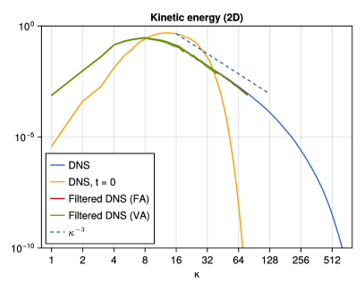
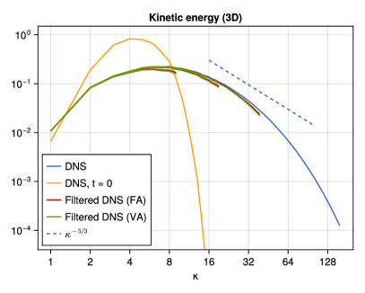
Figure 7: Kinetic energy spectra of DNS and filtered DNS at final time. The spectrum $\hat{E}_{\kappa}$ is obtained by adding the components $\hat{E}_{k}$ contained in the dyadic bins $[\kappa/a,\kappa a]$ with $a=1.6$. The filters are both applied for $3$ different filter sizes $\bar{n}$, visible in the three sudden stops at the cut-off wavenumbers $\bar{n}/2$. Left: 2D simulation, with theoretical scaling $k^{-3}$. Right: 3D simulation, with theoretical scaling $k^{-5/3}$.

5.1.2 Filtered fields

Figure 8 shows the discrete curl $\nabla\times\varphi$ of various 2D fields $\varphi\in\{u(0),u,\bar{u},PF(u),\bar{P}\bar{F}(\bar{u}),c\}$ for the face-averaging filter with $\bar{N}=128^{2}$. We plot the curl since $\varphi$ is a vector field. Each pixel corresponds to a pressure volume, in which the curl is interpolated for visualization. The filtered field $\bar{u}$ in the top-right corner is clearly unable to represent all the sub-grid fluctuations seen in the DNS field $u$, but the large eddies of $u$ are still recognizable in $\bar{u}$. We stress again that the aim of our neural closure models is to reproduce $\bar{u}$, without having knowledge of the DNS field $u$. This will be shown in section 5.2.

Note in particular that the coarse grid right hand side $\bar{P}\bar{F}(\bar{u})$ contains small oscillations which make the discrete curl look grainy. These are due to the under-resolved central-difference discretization on the coarse grid, and are subsequently also present in the discrete commutator error $c$. The closure model $m$ thus has to predict the oscillations in $c$ in order to correct for those in $\bar{P}\bar{F}(\bar{u})$, using information from the smooth field $\bar{u}$ only. If $c$ was defined by filtering first and then discretizing, as is commonly done in LES, these oscillations would not be part of $c$ and other means of stabilization would be needed to correct for the oscillations in $\bar{P}\bar{F}(\bar{u})$, such as explicit LES [43, 20, 7] (where the filter is applied to the non-linear convective term in the LES right hand side). This problem has also been addressed in literature; for example, Geurts et al. [24] and Beck and Kurz [6] argue that all commutator errors should be modeled, and Stoffer et al. [67] show that instabilities in the high wavenumbers can occur if the discretization is not included in the commutator error.

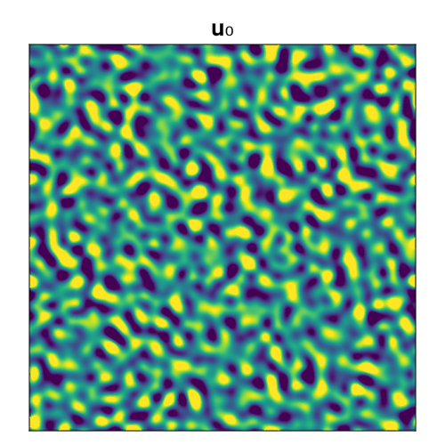
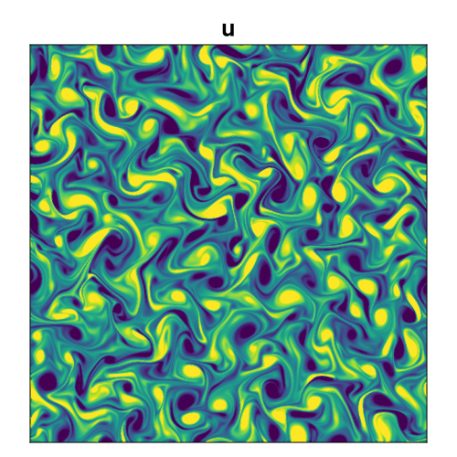
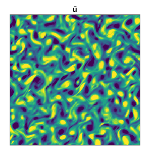
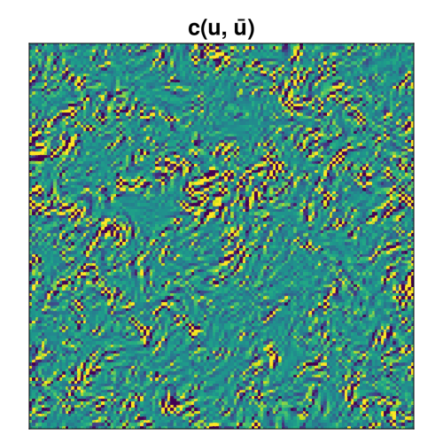
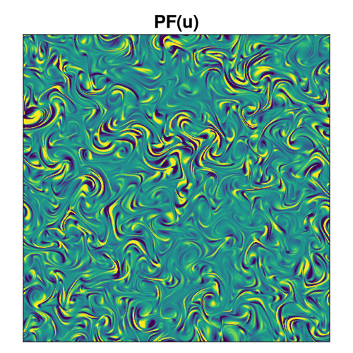
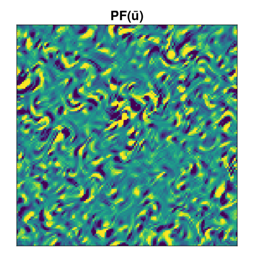
Figure 8: A-priori results: Discrete curl $-\delta_{2}\varphi^{1}+\delta_{1}\varphi^{2}$ of various 2D fields $\varphi\in\{u(0),u,\bar{u},PF(u),\bar{P}\bar{F}(\bar{u}),c(u,\bar{u})\}$. The filter is face-averaging, $\bar{N}=128^{2}$.

Figure 9 shows the vortex cores of the 3D simulation at initial and final time. The vortex cores are visualized as isocontours of $\lambda_{2}$-criterion [31]. It is defined as negative regions of $\lambda_{2}(S^{2}+T^{2})$, where $\lambda_{2}$ denotes the second largest eigenvalue in absolute value of the $3\times 3$-tensor, and $S=\frac{1}{2}(\nabla u+\nabla u^{\mathsf{T}})$ and $T=\frac{1}{2}(\nabla u-\nabla u^{\mathsf{T}})$ are the symmetric and anti-symmetric parts of the velocity gradient tensor. With the prescribed initial low wavenumber energy spectrum, only large DNS vortex structures are present at the initial time. They are clearly visible in the left plot. As energy gets transferred to higher wavenumbers, smaller turbulent vortex structures are formed (middle plot). The same DNS field still contains larger vortex structures, which become visible after filtering (right plot).

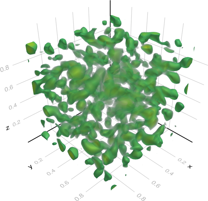
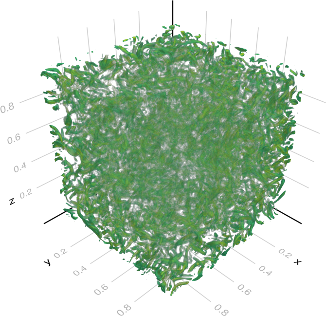
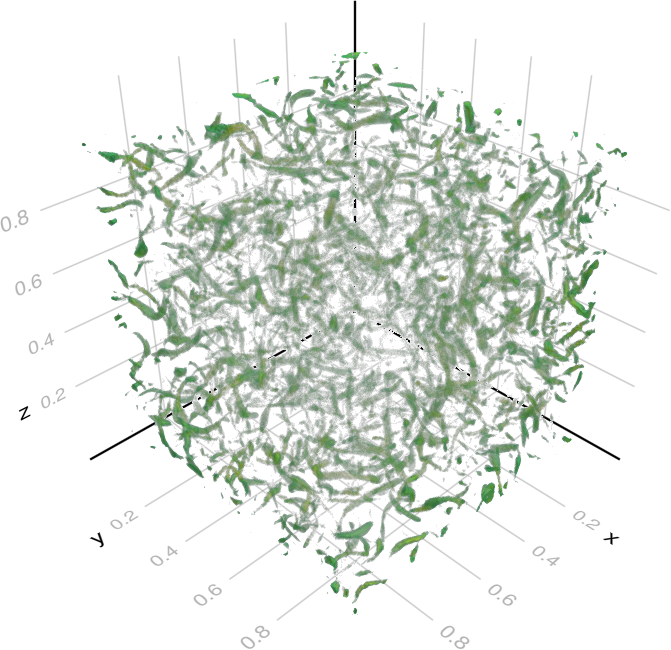
Figure 9: Vortex cores visualized as $10$ isocontours of negative regions of $\lambda_{2}(S^{2}+T^{2})$, where $\lambda_{2}$ denotes the second largest eigenvalue, and $S=\frac{1}{2}(\nabla u+\nabla u^{\mathsf{T}})$ and $T=\frac{1}{2}(\nabla u-\nabla u^{\mathsf{T}})$ are the symmetric and anti-symmetric parts of the velocity gradient. Left: DNS, initial time. Middle: DNS, final time. Right: Filtered DNS (face-averaging, $\bar{N}=128^{3}$), final time.

5.1.3 Divergence, commutator errors, and kinetic energy

Table 2 shows the magnitude of various quantities derived from the two DNS trajectories. All quantities $q(u(t))$ are averaged over time with a frequency of $s=20$ time steps as follows:

$$\langle q\rangle_{s}=\frac{1}{n_{t}/s+1}\sum_{i=0}^{n_{t}/s}q(u(t_{si})).$$ (31)

The considered quantities $q(u)$ are: Normalized divergence $\frac{\|\bar{D}\bar{u}\|}{\|\bar{u}\|}$, magnitude of non-divergence-free part of filtered velocity field $\frac{\|\bar{u}-\bar{P}\bar{u}\|}{\|\bar{u}\|}$, magnitude of non-divergence-free part of commutator error $\frac{\|c-\bar{P}c\|}{\|c\|}$, magnitude of commutator error in the total filtered right hand side $\frac{\|c\|}{\|\bar{P}\bar{F}+\bar{c}\|}$, and resolved kinetic energy $\frac{\|\bar{u}\|^{2}_{\bar{\Omega}}}{\|u\|^{2}_{\Omega}}$. The norms are defined as $\|u\|=\sqrt{\sum_{\alpha=1}^{d}\|u^{\alpha}\|^{2}}$ for vector fields such as $u$ and $\|u^{\alpha}\|=\sqrt{\sum_{I}|u^{\alpha}_{I}|^{2}}$ for scalar fields such as $u^{\alpha}$. Additionally, the norm $\|\cdot\|_{\Omega}$ is weighted by the volume sizes.

$N$	Filter	$\bar{N}$	$\frac{\|\bar{D}\bar{u}\|}{\|\bar{u}\|}$	$\frac{\|\bar{u}-\bar{P}\bar{u}\|}{\|\bar{u}\|}$	$\frac{\|c-\bar{P}c\|}{\|c\|}$	$\frac{\|c\|}{\|\bar{P}\bar{F}+c\|}$	$\frac{\|\bar{u}\|^{2}_{\bar{\Omega}}}{\|u\|^{2}_{\Omega}}$
$4096^{2}$	FA	$\phantom{0}64^{2}$	$2.2\times 10^{-14}$	$2.1\times 10^{-16}$	$1.0\times 10^{-13}$	$0.58$	$0.91$
	FA	$128^{2}$	$3.2\times 10^{-14}$	$1.7\times 10^{-16}$	$1.7\times 10^{-13}$	$0.30$	$0.98$
	FA	$256^{2}$	$5.0\times 10^{-14}$	$1.5\times 10^{-16}$	$3.9\times 10^{-13}$	$0.13$	$0.99$
	VA	$\phantom{0}64^{2}$	$2.0\phantom{0}$	$0.017\phantom{0}$	$0.090$	$0.57$	$0.88$
	VA	$128^{2}$	$1.1\phantom{0}$	$0.0055$	$0.078$	$0.30$	$0.97$
	VA	$256^{2}$	$0.54$	$0.0017$	$0.086$	$0.13$	$0.99$
$512^{3}$	FA	$\phantom{0}32^{3}$	$2.0\times 10^{-14}$	$2.6\times 10^{-16}$	$1.9\times 10^{-14}$	$0.54$	$0.86$
	FA	$\phantom{0}64^{3}$	$2.0\times 10^{-14}$	$1.4\times 10^{-16}$	$4.4\times 10^{-14}$	$0.36$	$0.95$
	FA	$128^{3}$	$2.1\times 10^{-14}$	$7.9\times 10^{-17}$	$1.3\times 10^{-13}$	$0.20$	$0.99$
	VA	$\phantom{0}32^{3}$	$1.4\phantom{0}$	$0.020\phantom{0}$	$0.11$	$0.52$	$0.83$
	VA	$\phantom{0}64^{3}$	$1.2\phantom{0}$	$0.0093$	$0.14$	$0.35$	$0.94$
	VA	$128^{3}$	$0.88$	$0.0039$	$0.23$	$0.20$	$0.98$

Table 2: Magnitude of various quantities derived from two DNS trajectories $u(t)$ (one in 2D, one in 3D). All quantities are averaged over time.

It is clear that both $\bar{u}$ and $c$ are divergence-free for the face-averaging filter, in both 2D and 3D. For the volume-averaging filter on the other hand, $\bar{u}$ and $\bar{c}$ are not divergence-free. At $\bar{N}=64^{2}$, the orthogonal projected part $\bar{u}-\bar{P}\bar{u}$ comprises about $1.7\%$ of $\bar{u}$. This is more visible for the commutator error, for which the orthogonal part is $9\%$ of the total commutator error. When the grid is refined to $\bar{N}=256^{2}$ however, the non-divergence-free parts of $\bar{u}$ and $c$ shrink to $0.17\%$ and $8.6\%$ since the flow is more resolved. For $\bar{N}=32^{3}$, the non-divergence free parts of $\bar{u}$ and $c$ are $2.3\%$ and $11\%$ respectively. While the one of $\bar{u}$ shrinks to $0.39\%$ for $\bar{N}=128^{3}$, the one of $c$ increases to $23\%$ since $c$ itself becomes smaller. Note that the volume-averaging filter width was chosen to be equal to the grid spacing, but these divergence errors would be larger if we increased the filter width.

For both 2D and 3D, and both filters types, the commutator error becomes smaller when the grid is refined, which is expected since more scales are resolved. The commutator error magnitude does not seem to depend much on whether we use face-averaging or volume-averaging, since they both have the same characteristic filter width. For $\bar{N}=64^{2}$ and $\bar{N}=32^{3}$, more than half of the total right hand side is due to the commutator error, even though $91\%$ and $86\%$ of the kinetic energy is resolved by $\bar{u}$. For these resolutions, it is very important to have a good closure model. For $\bar{N}=256^{2}$, the filtered DNS right hand side is much closer to the corresponding coarse unfiltered DNS right hand side, with $c$ comprising $13\%$ of the total right hand side $\bar{P}\bar{F}+c$. A closure model is still clearly needed, even though $99\%$ of the energy being resolved by $\bar{u}$. Bae et al. [2] also found the discretization part of the commutator errors to be quite significant, in particular near walls (which we do not consider in this study).

In summary, the DNS and filtered DNS results confirm the theoretical analysis in section 3.3. The volume-averaging filter lacks divergence-consistency of the solution and the closure term. The magnitude of the closure term is similar for both filters. The benefits of divergence-consistency will be demonstrated in the a-posteriori analysis in the subsequent section.

5.2 LES (2D)

Next, we turn to the results for the key challenge set out in this paper: testing our neural closure models in an LES setting, with divergence-consistent filters, aiming to approximate the trajectory $\bar{u}(t)$ given $\bar{u}(0)$. We now only consider the 2D problem to reduce the computational time, since the same network is trained repeatedly in multiple configurations. The DNS resolution is set to $N=(4096,4096)$. The Reynolds number is $\mathrm{Re}=10^{4}$. The initial peak wavenumber is $\kappa_{p}=20$. We use single precision floating point numbers for all computations, including DNS trajectory generation, to reduce memory usage and increase speed. Details about the datasets are found in D.3.

For the closure model $m$, we consider three options:

1. No closure model, $m_{0}=0$. This is the baseline model.

2. Smagorinsky closure model, $m_{\text{S}}$.

3. Convolutional neural closure model, $m_{\text{CNN}}$. The architecture is shown in D.4.

See D.5 for details about the training.

5.2.1 A-priori errors

Figure 10 shows the average relative a-priori errors $\frac{1}{n_{\text{u}}}\sum_{u}\frac{\|m-c\|}{\|c\|}$ for the testing dataset and the three CNN parameters $\theta^{\text{prior}}$, $\theta^{\text{post}}_{\text{DIF}}$, and $\theta^{\text{post}}_{\text{DCF}}$. For the no-closure model $m_{0}$, the a-priori error is always $\|0-c\|/\|c\|=1$. For both FA and VA and for all grid sizes, the a-priori trained parameters $\theta^{\text{prior}}$ perform the best. This is expected, since the a-priori loss function used to obtain $\theta^{\text{prior}}$ is similar to the a-priori error.

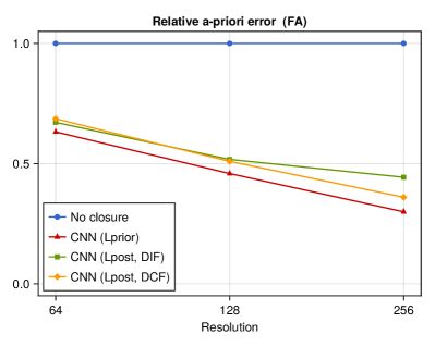
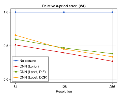
Figure 10: A-priori errors $\frac{1}{n_{\text{u}}}\sum_{u}\frac{\|m-c\|}{\|c\|}$ for the testing dataset. Left: Face-averaging filter. Right: Volume-averaging filter.

5.2.2 A-posteriori errors

The relative a-posteriori error $\frac{1}{n_{t}}\sum_{i=1}^{n_{t}}\|\bar{v}_{i}-\bar{u}_{i}\|/\|\bar{u}_{i}\|$ is computed for the trajectory in the testing dataset. A CNN parameter set $\theta$ is only used for testing on the same coarse grid and same filter type that it was trained for. Figure 11 shows the average error over time.

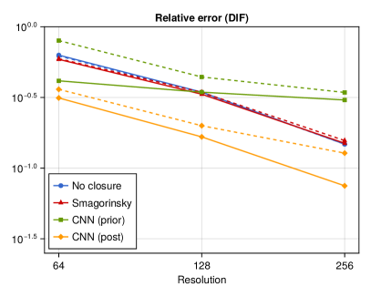
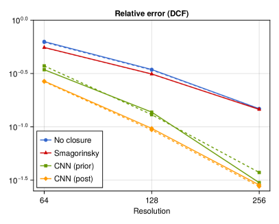
Figure 11: A-posteriori errors $\frac{1}{n_{t}}\sum_{i=1}^{n_{t}}\|\bar{v}_{i}-\bar{u}_{i}\|/\|\bar{u}_{i}\|$ for the testing dataset. The CNN is trained separately for each resolution and each filter type with $L^{\text{prior}}$ (green squares) and $L^{\text{prior}}$-then-$L^{\text{post}}$ (yellow diamonds). Solid lines: Face-averaging ($\Phi^{\text{FA}}$). Dashed lines: Volume-averaging ($\Phi^{\text{VA}}$). Left: General model $\mathcal{M}_{\text{DIF}}$. Right: Divergence-consistent model $\mathcal{M}_{\text{DCF}}$.

For $\mathcal{M}_{\text{DCF}}$ (right), the no-closure and the Smagorinsky closure have similar errors, with $m_{\text{S}}$ performing slightly better for low LES-resolutions. The CNN is clearly outperforming the other two closures. The errors for the face-average and volume-average filters are indistinguishable, except for $\theta^{\text{prior}}$ at $\bar{n}=256$. The accuracy of the CNN increases when using the parameters obtained from a-posteriori training. Note that this training is done starting from the best performing a-priori trained parameters.

For $\mathcal{M}_{\text{DIF}}$ (left), the no-closure and the Smagorinsky closure have similar profiles as for $\mathcal{M}_{\text{DCF}}$. For the no-closure, the two LES formulations are actually identical. For FA at $\bar{n}=256$, and at all resolutions for VA, $m_{\text{CNN}}(\cdot,\theta^{\text{prior}})$ is showing signs of instability and is performing worse than $m_{0}$. The a-posteriori training does however seem to have corrected for these errors. The closure $m_{\text{CNN}}(\cdot,\theta^{\text{post}}_{\text{DIF}})$ is performing better than $m_{0}$ and $m_{\text{S}}$. In addition, FA produces visibly lower errors than VA for both training procedures.

5.2.3 Stability

To further investigate the stability, we compute the evolution of the total kinetic energy as a function of time. This is shown in figure 12. In terms of total energy, the no-closure solution is dissipating more energy than the reference solution. The Smagorinsky closure is even more dissipative, which is well known for the standard Smagorinsky model. For $\mathcal{M}_{\text{DCF}}$, the CNN has a similar profile as the reference. For $\mathcal{M}_{\text{DIF}}$, the high CNN errors from figure 11 are confirmed by the rapid growth of the total kinetic energy. Similar growth in energy of unconstrained neural closure models after a period of seemingly good overlap with the reference energy has been observed by Beck and Kurz [4, 35], although in a different configuration. Training with $L^{\text{post}}$ improves the stability, and the energy stays close to the reference for a longer period. This was not sufficient to stabilize $\mathcal{M}_{\text{DIF}}$, however, and the energy eventually starts increasing.

The growth in kinetic energy and resulting lack of stability for the divergence-inconsistent model can be explained by the energy-conservation properties of our spatial discretization. The convective terms are discretized with a second order central scheme (in so-called divergence form), which can be shown to be equivalent to a skew-symmetric, energy-conserving form provided that the velocity field is divergence-free [71]. If the velocity field is not divergence-free, there is no guarantee that the convective terms are energy-conserving, which can lead to growth in kinetic energy and loss of stability.

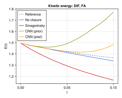
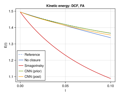
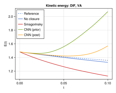
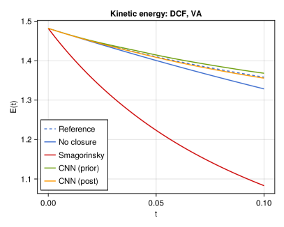
Figure 12: Total kinetic energy evolution for $\bar{n}=128$. Left: Unprojected closure model $\mathcal{M}_{\text{DIF}}$. Right: Constrained model $\mathcal{M}_{\text{DCF}}$. Top: Face-averaging filter. Bottom: Volume-averaging filter.

5.2.4 Energy spectra

The energy spectra at the final time are shown in figure 13. The no-closure model spectrum is generally close to the reference spectrum, but contains too much energy in the high wavenumbers. This is likely due to the oscillations discussed in the previous sections. The Smagorinsky closure is correcting for this (as intended), but is also dissipating too much energy overall. For $\mathcal{M}_{\text{DCF}}$, the a-posteriori trained CNN spectrum is visually very close to the reference spectrum. For $\mathcal{M}_{\text{DIF}}$, all the closure models produce too much energy in the high wave numbers. This is also the case for the Smagorinsky model, although it is even more so for the CNN. Training with $L^{\text{post}}$ seems to improve this somewhat.

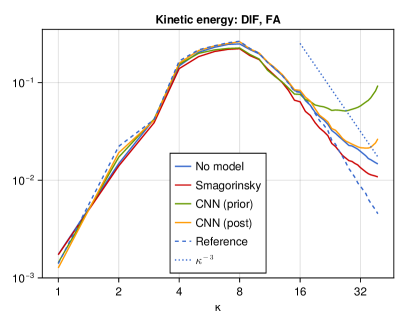
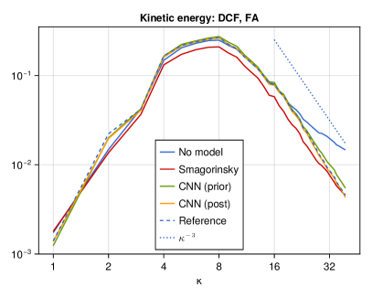
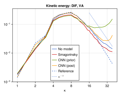
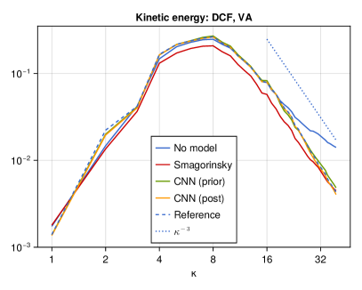
Figure 13: Energy spectra at final time for $\bar{n}=128$. Left: General model $\mathcal{M}_{\text{DIF}}$. Right: Divergence-consistent model $\mathcal{M}_{\text{DCF}}$. Top: Face-averaging filter. Bottom: Volume-averaging filter.

5.2.5 LES solution fields

The curl of the LES solutions (LES vorticity) at the final time is shown in figure 14. The reference solution $\bar{u}$ has a smooth vorticity field for all resolutions, since the low-pass filtering operation removes high wavenumber components. The no-closure model solution, on the other hand, shows sharp oscillations. Only the initial conditions are smooth, since $\bar{v}(0)=\bar{u}(0)$. As the solution evolves in time, the central difference scheme used in the right hand side $\bar{P}\bar{F}$ is too coarse for the given Reynolds numbers, and produces well known oscillations [62]. For the highest resolution $\bar{n}=256$, these oscillations go away, and $\bar{v}$ starts visually resembling $\bar{u}$.

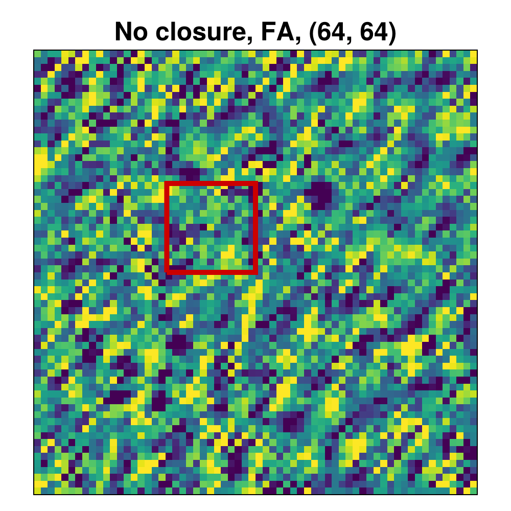
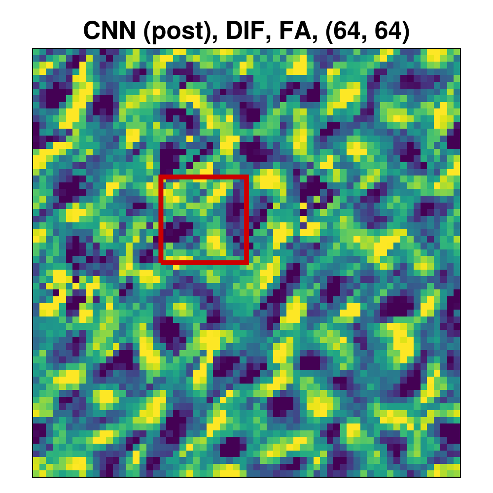
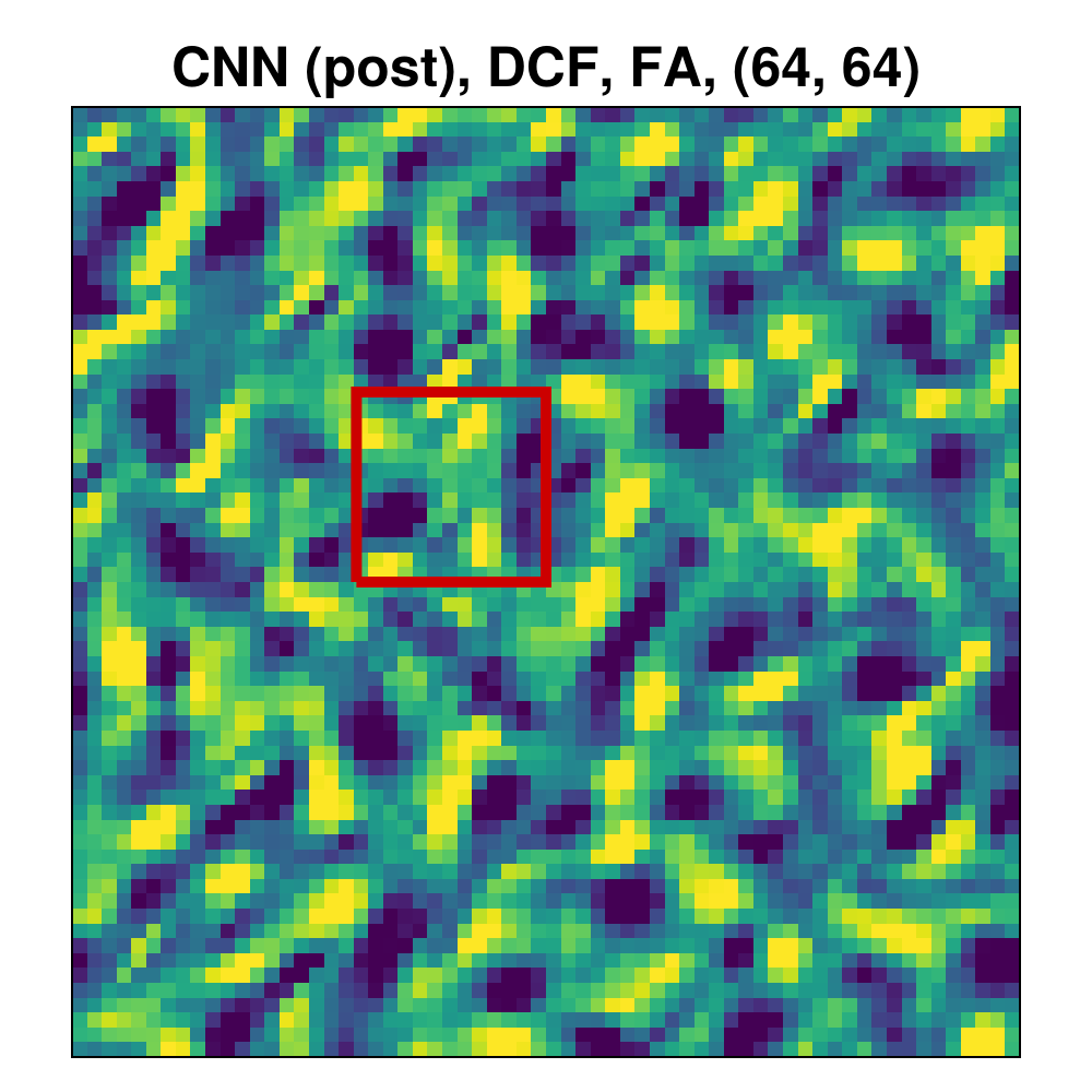
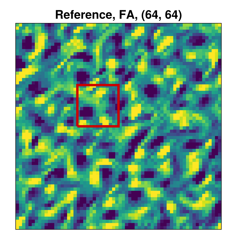
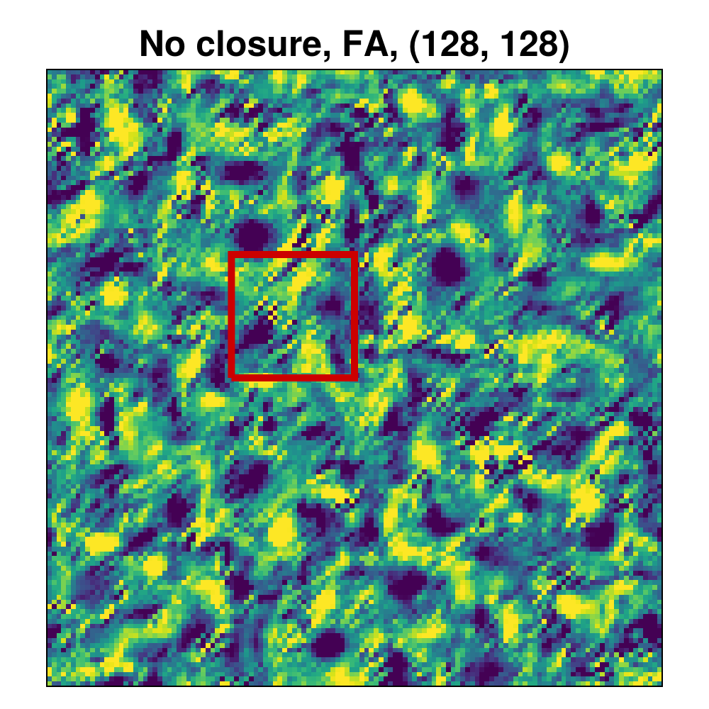
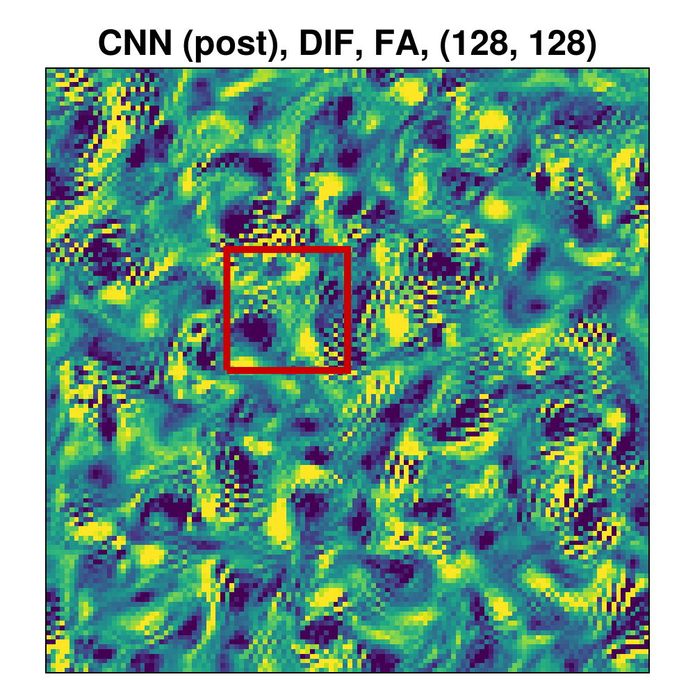
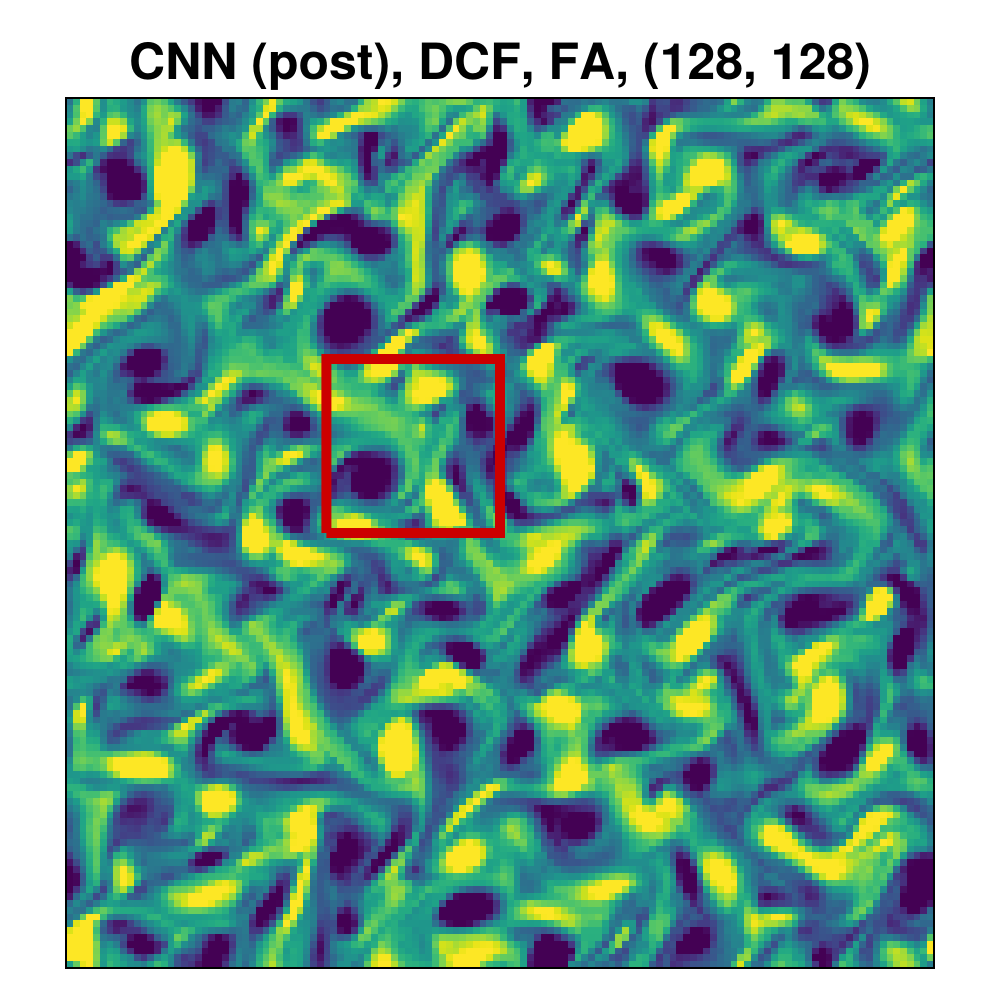
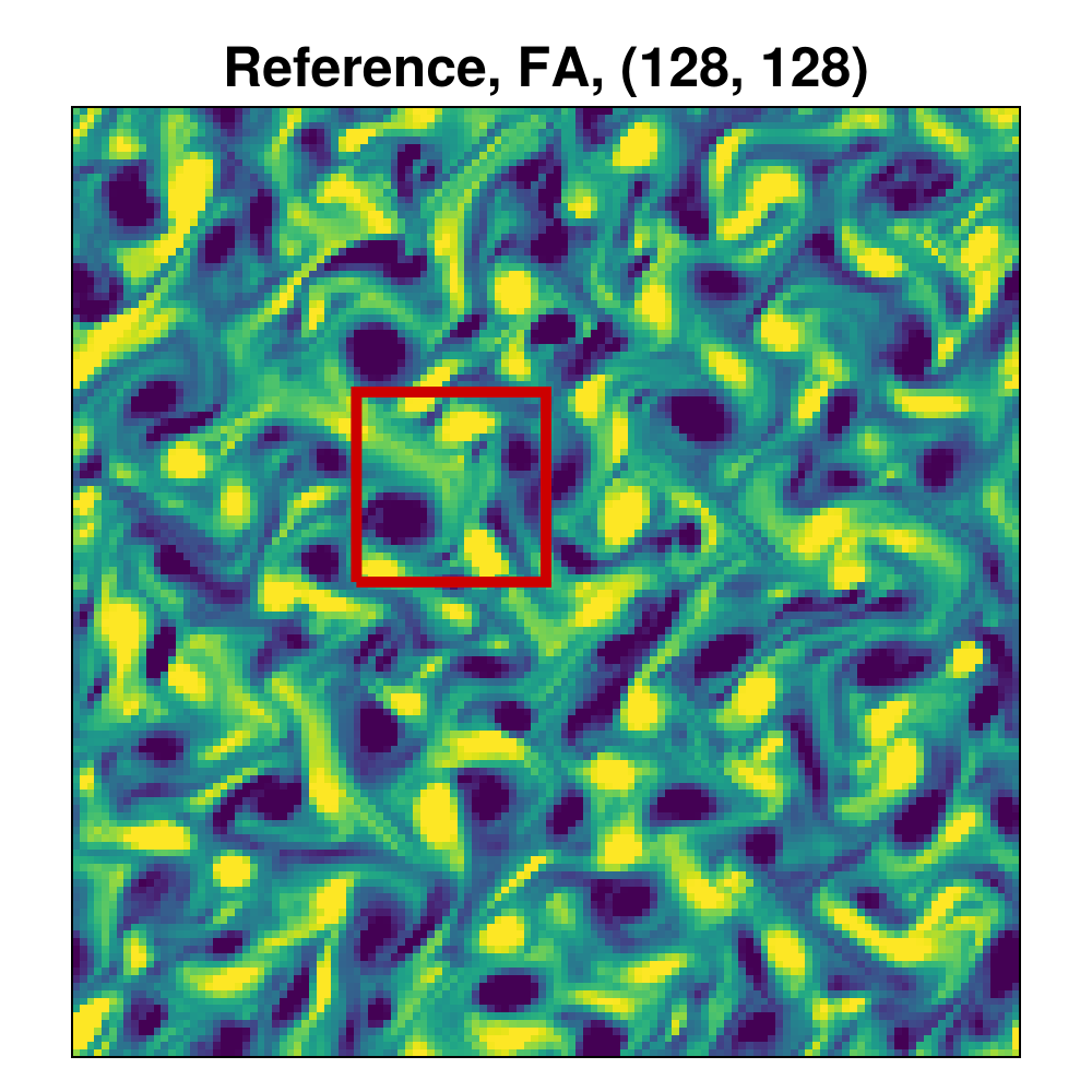
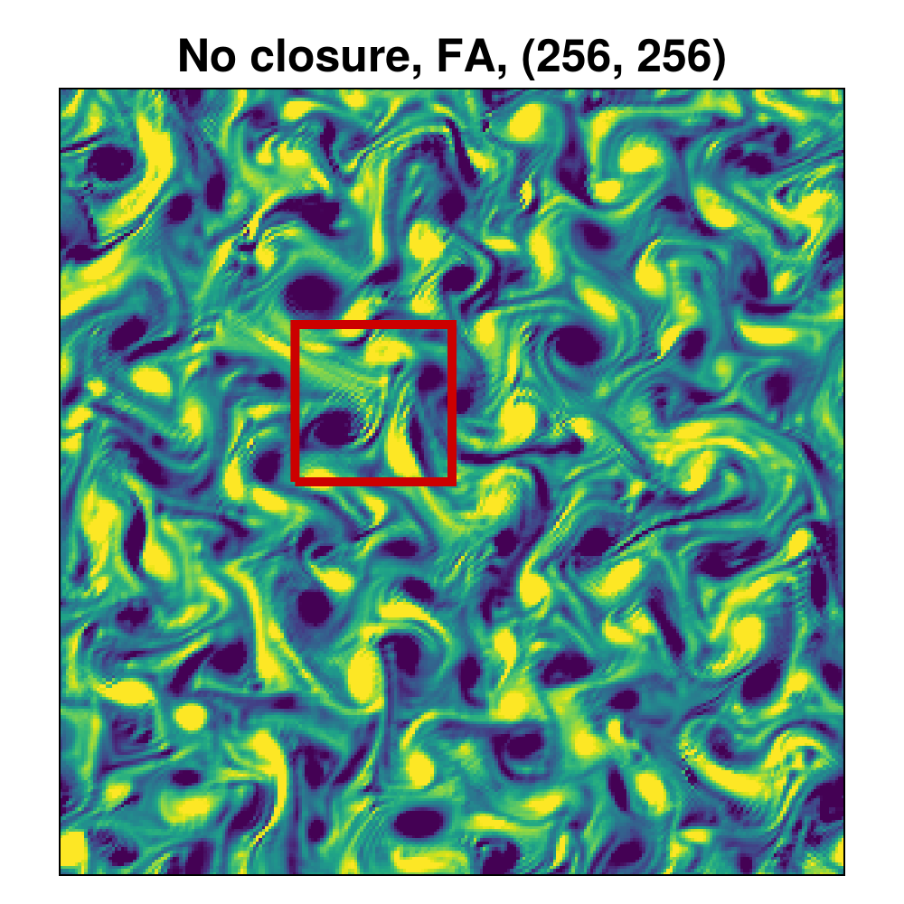
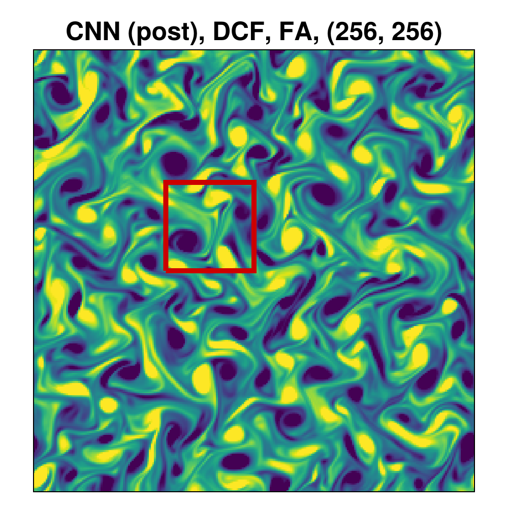
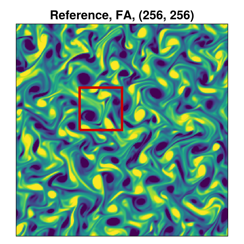
Figure 14: Vorticity of filtered DNS solution $\bar{u}$ (right) and LES solutions $\bar{v}$ computed using no closure (first column), $\mathcal{M}_{\text{DIF}}$ (second column), and $\mathcal{M}_{\text{DCF}}$ (third column) at final time for testing trajectory for $\bar{n}=64$ (top), $\bar{n}=128$ (middle), and $\bar{n}=256$ (bottom).

Adding an $\mathcal{M}_{\text{DCF}}$ constrained CNN closure term trained using $L^{\text{post}}_{\text{DCF}}$ seems to correct for the oscillations of the no-closure model, and we recover the smooth fields with recognizable features from the reference solution (compare $\bar{u}$ and $\bar{v}$ inside the red square). We are effectively doing large eddy simulation, as large eddies are visually found in the right positions after simulation. However, if we remove the projection and use the $\mathcal{M}_{\text{DIF}}$ CNN closure model, the solution becomes unstable, even after accounting for this by training with $L^{\text{post}}_{\text{DIF}}$. This confirms the observations from figure 11.

We stress again that the CNN closure model is accounting for the total commutator error resulting from the discrete filtering procedure. This commutator error includes the coarse grid discretization error, and also the oscillations produced by the central difference scheme.

5.2.6 Divergence

Figure 15 shows the evolution of the average divergence $\sqrt{\frac{1}{\bar{N}}\sum_{I}(\bar{D}\bar{v})_{I}^{2}}$ for the two LES models $\mathcal{M}_{\text{DIF}}$ and $\mathcal{M}_{\text{DCF}}$.

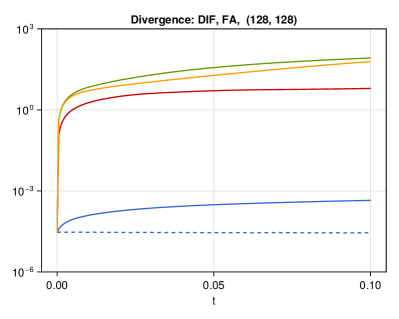
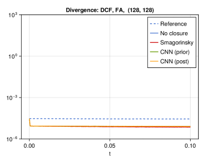
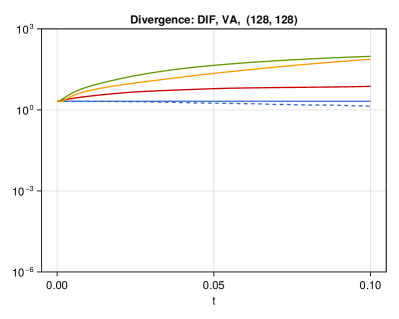
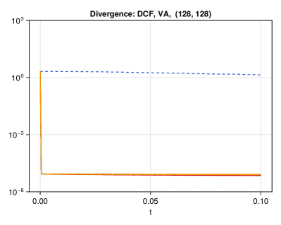
Figure 15: Divergence evolution for $\bar{n}=128$. Top: Face-averaging filter. Bottom: Volume-averaging filter. Left: Unprojected LES model $\mathcal{M}_{\text{DIF}}$. Right: Constrained LES model $\mathcal{M}_{\text{DCF}}$.

For the face-averaging filter, the filtered DNS divergence (reference) is of the order of $10^{-5}$ due to the single precision arithmetic. For $\mathcal{M}_{\text{DIF}}$, all closure models produce a divergence increasing in time. This is likely due to the instability observed in the previous figures. For $\mathcal{M}_{\text{DCF}}$, all closure models produce divergences at the same order of magnitude as the reference, since the solution is projected at every time step.

For the volume-averaging filter, the filtered DNS divergence (reference) is of the order of $1$, since $\Phi^{\text{VA}}$ does not preserve the divergence constraint. For $\mathcal{M}_{\text{DIF}}$, all closure models produce an increasing divergence, just like for $\Phi^{\text{FA}}$. For $\mathcal{M}_{\text{DCF}}$, all closure models produce divergence free solutions, even though the reference solution is actually not divergence-free.

5.2.7 Computational cost

The computational time for generating filtered DNS data and training the neural networks is shown in table 3. Only one DNS is necessary for all filter combinations. The two models $\mathcal{M}_{\text{DIF}}$ and $\mathcal{M}_{\text{DCF}}$ bot produce similar timings, as exactly the same number of operations are performed (but in a different order). The similar times for $L^{\text{post}}$ at $\bar{n}=64$ and $\bar{n}=128$ are likely due to the fact that the same number of time steps are unrolled for all LES resolutions, resulting in an equal number of GPU kernel calls. Since $64^{2}$ and $128^{2}$ are both relatively small, the kernels for the differential operators (convection, Poisson solves, etc.) do not show any improvement for the lower resolution. This does not seem to be the case for the $L^{\text{prior}}$ training however, where most of the kernel calls are to the highly optimized convolutional operators in CUDNN [14].

$\bar{u}$	Filter	$\bar{n}$	$L^{\text{prior}}$	$L^{\text{post}}_{\text{DIF}}$	$L^{\text{post}}_{\text{DCF}}$
$1501.1$	FA	$\phantom{0}64$	$\phantom{0}125.0$	$1281.9$	$1281.7$
	FA	$128$	$\phantom{0}283.7$	$1256.8$	$1256.3$
	FA	$256$	$1026.0$	$1774.3$	$1760.6$
	VA	$\phantom{0}64$	$\phantom{0}\phantom{0}95.3$	$1281.2$	$1281.9$
	VA	$128$	$\phantom{0}282.2$	$1255.2$	$1256.9$
	VA	$256$	$1026.2$	$1774.4$	$1760.3$

Table 3: Computational time (in seconds) for DNS and filtering of training, validation, and testing data ($\bar{u}$), a-priori training for 10000 iterations ($L^{\text{prior}}$), and a-posteriori training for 2000 iterations ($L^{\text{post}}$).

The benefit of a-posteriori training is clear in situations where the a-priori trained model is unstable (in our case: $\mathcal{M}_{\text{DIF}}$), but for a-priori trained models that are stable and accurate (such as $\mathcal{M}_{\text{DCF}}$), one could ask whether the additional cost of a-posteriori training is worth it. We think the additional accuracy is useful, since the learned weights can be reused without having to retrain the model, as long as the same configuration is used (grid size, Reynolds number etc.).

6 Conclusion

The use of neural networks for LES closure models is a promising approach. Neural networks are discrete by nature, and thus require consistent discrete training data. To achieve model-data consistency, we propose the paradigm “discretize, differentiate constraint, filter, and close” (in that particular order). This ensures full model-data consistency and circumvents pressure problems. We do not need to define a pressure filter, only a velocity filter is needed. Our framework allows for training the neural closure model using a-priori loss functions, where the model is trained to predict the target commutator error directly, or using a-posteriori loss functions, where the model is trained to approximate the target filtered DNS-solution trajectory.

To ensure that the filtered DNS velocity stays divergence-free, we introduced a novel divergence-consistent discrete filter using face-averaging. This allows for using a divergence-constrained LES model similar to those commonly used in LES, but with the important difference that the training data obtained through discrete DNS is fully consistent with the LES environment. This resulted in our new divergence-consistent LES model, which was found to be stable with both a-priori and a-posteriori training. A-posteriori training is more expensive than a-priori training, but still has the advantage of increased accuracy.

Our divergence-consistent filter stands out from commonly used (volume-averaging) discrete filters, for which the filtered DNS solution is generally not divergence-free. We showed that the resulting LES model can produce instabilities. A-posteriori trained models were found to improve the stability over a-priori trained models, but this was not sufficient to fully stabilize the model in our experiment. With our face-averaging filter, such instability issues did not occur.

Another important property of our approach is that the (coarse grid) discretization error is included in the training data and learned by the neural network. Turbulence simulations with DNS and LES rely on non-dissipative discretization methods, such as the second order central difference discretization we used in this work, but they produce oscillations and instabilities on coarse grids. This could limit their use in LES, where using coarse grids is one of the main goals. Various smoothing methods, such as explicit LES or (overly) diffusive closure models are commonly used to address this issue. We let the closure model learn to account for the oscillations. The fact that the coarse grid discretization effects (and thus the oscillations) are included in the training data allows the neural network to recognize and correct for these oscillations, even when training with a-priori loss functions.

We realize that the choice of a divergence-consistent face-averaging filter imposes some constraints on the filter choice. The weights have to be uniform (top-hat filter like) to ensure that all the sub-filter velocities cancel out, and the extension to other filters like Gaussians is an open problem. In addition, we took the filter width to be equal to the grid spacing. The face-average filter naturally extends to unstructured grids, as shown in figure 2. However, this requires that the DNS grid perfectly overlaps with the faces of the LES grid. This can be achieved by designing the DNS and LES grids at the same time. Lastly, our proposed filter is only divergence-consistent with respect to the second-order central difference divergence operator on a staggered grid. We intend to explore the use of filters that are divergence-consistent with respect to higher-order discretization methods (such as the discontinuous Galerkin element method) and non-staggered grids.

Future work will include the use of non-uniform grids with solid walls boundary conditions. This modification will require a change in the neural network architecture, but not in the face-averaging filtering procedure itself. The CNN architecture assumes that the grid is uniform, but weighting the kernel stencil with non-uniform volume sizes could be a way to design a discretization-informed neural network. We intend to exploit the fact that discrete DNS boundary conditions naturally extend to the LES model for the face-average filter. We also intend to incorporate other constraints into the LES model, such as conservation of quantities of interest, in particular kinetic energy conservation, as studied in [70].

Software and reproducibility statement

The Julia scripts and source code used to generate all the results are available at
https://github.com/agdestein/IncompressibleNavierStokes.jl.
It is released under the MIT license. Most simulations were run on an Nvidia RTX 4090 GPU. The 3D simulation from section 5.1 was run on an Nvidia A100 GPU (with 40 gigabytes of memory), as the double precision floating point numbers required additional memory.

To produce the results of this article, pseudo-random numbers were used for

• data generation (DNS initial conditions for training, validation, and testing data);

• neural network parameter initialization;

• batch selection during stochastic gradient descent.

The scripts include the seeding numbers used to initialize the pseudo-random number generators. Given a seeded pseudo-random generator, the code is deterministic and the results are reproducible.

CRediT author statement

Syver Døving Agdestein: Conceptualization, Methodology, Software, Validation, Visualization, Writing – Original Draft

Benjamin Sanderse: Formal analysis, Funding acquisition, Project administration, Supervision, Writing – Review & Editing

Declaration of Generative AI and AI-assisted technologies in the writing process

During the preparation of this work the authors used GitHub Copilot in order to propose wordings and mathematical typesetting. After using this tool/service, the authors reviewed and edited the content as needed and take full responsibility for the content of the publication.

Declaration of competing interest

The authors declare that they have no known competing financial interests or personal relationships that could have appeared to influence the work reported in this paper.

Appendix A Finite volume discretization

In this work, the integral form of the Navier-Stokes equations is considered, which is used as starting point to develop a spatial discretization:

$$\frac{1}{|\mathcal{O}|}\int_{\partial\mathcal{O}}u\cdot n\,\mathrm{d}\Gamma =0,$$ (32)

$$\frac{\mathrm{d}}{\mathrm{d}t}\frac{1}{|\mathcal{O}|}\int_{\mathcal{O}}u\,\mathrm{d}\Omega =\frac{1}{|\mathcal{O}|}\int_{\partial\mathcal{O}}\left(-uu^{\mathsf{T}}-pI+\nu\nabla u\right)\cdot n\,\mathrm{d}\Gamma+\frac{1}{|\mathcal{O}|}\int_{\mathcal{O}}f\mathrm{d}\Omega,$$ (33)

where $\mathcal{O}\subset\Omega$ is an arbitrary control volume with boundary $\partial\mathcal{O}$, normal $n$, surface element $\mathrm{d}\Gamma$, and volume size $|\mathcal{O}|$. We have divided by the control volume sizes in the integral form, so that system (32)-(33) has the same dimensions as the system (1)-(2).

A.1 Staggered grid configuration

In this section we describe a finite volume discretization of equations (32)-(33). Before doing so, we introduce our notation, which is such that the mathematical description of the discretization closely matches the software implementation.

The $d$ spatial dimensions are indexed by $\alpha\in\{1,\dots,d\}$. The $\alpha$-th unit vector is denoted $2h_{\alpha}=(2h_{\alpha\beta})_{\beta=1}^{d}$, where the (half) Kronecker symbol $h_{\alpha\beta}$ is $1/2$ if $\alpha=\beta$ and $0$ otherwise. The Cartesian index $I=(I_{1},\dots,I_{d})$ is used to avoid repeating terms and equations $d$ times, where $I_{\alpha}$ is a scalar index (typically one of $i$, $j$, and $k$ in common notation). This notation is dimension-agnostic, since we can write $u_{I}$ instead of $u_{ij}$ in 2D or $u_{ijk}$ in 3D. In our Julia implementation of the solver we use the same Cartesian notation (u[I] instead of u[i, j] or u[i, j, k]).

For the discretization scheme, we use a staggered Cartesian grid as proposed by Harlow and Welch [28]. Staggered grids have excellent conservation properties [39, 53], and in particular their exact divergence-freeness is important for this work. Consider a rectangular domain $\Omega=\prod_{\alpha=1}^{d}[a_{\alpha},b_{\alpha}]$, where $a_{\alpha}<b_{\alpha}$ are the domain boundaries and $\prod$ is a Cartesian product. Let $\Omega=\bigcup_{I\in\mathcal{I}}\Omega_{I}$ be a partitioning of $\Omega$, where $\mathcal{I}=\prod_{\alpha=1}^{d}\{\frac{1}{2},2-\frac{1}{2},\dots,N_{\alpha}-\frac{1}{2}\}$ are volume center indices, $N=(N_{1},\dots,N_{d})\in\mathbb{N}^{d}$ are the number of volumes in each dimension, $\Omega_{I}=\prod_{\alpha=1}^{d}\Delta^{\alpha}_{I_{\alpha}}$ is a finite volume, $\Gamma^{\alpha}_{I}=\Omega_{I-h_{\alpha}}\cap\Omega_{I+h_{\alpha}}=\prod_{\beta\neq\alpha}\Delta^{\beta}_{I_{\beta}}$ is a volume face, $\Delta^{\alpha}_{i}=\left[x^{\alpha}_{i-\frac{1}{2}},x^{\alpha}_{i+\frac{1}{2}}\right]$ is a volume edge, $x^{\alpha}_{0},\dots,x^{\alpha}_{N_{\alpha}}$ are volume boundary coordinates, and $x^{\alpha}_{i}=\frac{1}{2}\left(x^{\alpha}_{i-\frac{1}{2}}+x^{\alpha}_{i+\frac{1}{2}}\right)$ for $i\in\{1/2,\dots,N_{\alpha}-1/2\}$ are volume center coordinates. We also define the operator $\delta_{\alpha}$ which maps a discrete scalar field $\varphi=(\varphi_{I})_{I}$ to

$$(\delta_{\alpha}\varphi)_{I}=\frac{\varphi_{I+h_{\alpha}}-\varphi_{I-h_{\alpha}}}{|\Delta^{\alpha}_{I_{\alpha}}|}.$$ (34)

It can be interpreted as a discrete equivalent of the continuous operator $\frac{\partial}{\partial x^{\alpha}}$. All the above definitions are extended to be valid in volume centers $I\in\mathcal{I}$, volume faces $I\in\mathcal{I}+h_{\alpha}$, or volume corners $I\in\mathcal{I}+\sum_{\alpha=1}^{d}h_{\alpha}$. The discretization is illustrated in figure 16.

Figure 16: Finite volume discretization on a staggered grid. Note that the grid can be non-uniform, as long as each volume in a given column has the same width and each volume in a given row has the same height. Here, $I$ and $J$ are two arbitrary Cartesian indices, with $I\in\mathcal{I}$ in a volume center and $J\in\mathcal{I}+h_{1}+h_{2}$ in a volume corner for illustrative purposes.

A.2 Equations for unknowns

We now define the unknown degrees of freedom. The average pressure in $\Omega_{I}$, $I\in\mathcal{I}$ is approximated by the quantity $p_{I}(t)$. The average $\alpha$-velocity on the face $\Gamma^{\alpha}_{I}$, $I\in\mathcal{I}+h_{\alpha}$ is approximated by the quantity $u^{\alpha}_{I}(t)$. Note how the pressure $p$ and the $d$ velocity fields $u^{\alpha}$ are each defined in their own canonical positions $x_{I}$ and $x_{I+h_{\alpha}}$ for $I\in\mathcal{I}$. This is illustrated for a given volume $I$ in figure 16. In the following, we derive equations for these unknowns.

Using the pressure control volume $\mathcal{O}=\Omega_{I}$ with $I\in\mathcal{I}$ in the integral constraint (32) and approximating the face integrals with the mid-point quadrature rule $\int_{\Gamma_{I}}u\,\mathrm{d}\Gamma\approx|\Gamma_{I}|u_{I}$ results in the discrete divergence-free constraint

$$\sum_{\alpha=1}^{d}(\delta_{\alpha}u^{\alpha})_{I}=0.$$ (35)

Note how dividing by the volume size results in a discrete equation resembling the continuous one (since $|\Omega_{I}|=|\Gamma^{\alpha}_{I}||\Delta^{\alpha}_{I_{\alpha}}|$).

Similarly, choosing an $\alpha$-velocity control volume $\mathcal{O}=\Omega_{I}$ with $I\in\mathcal{I}+h_{\alpha}$ in equation (33), approximating the volume- and face integrals using the mid-point quadrature rule, and replacing remaining spatial derivatives in the diffusive term with a finite difference approximation gives the discrete momentum equations

$$\frac{\mathrm{d}}{\mathrm{d}t}u^{\alpha}_{I}=-\sum_{\beta=1}^{d}(\delta_{\beta}(u^{\alpha}u^{\beta}))_{I}+\nu\sum_{\beta=1}^{d}(\delta_{\beta}\delta_{\beta}u^{\alpha})_{I}+f^{\alpha}(x_{I})-(\delta_{\alpha}p)_{I}.$$ (36)

where we made the assumption that $f$ is constant in time for simplicity. The outer discrete derivative in $(\delta_{\beta}\delta_{\beta}u^{\alpha})_{I}$ is required at the position $I$, which means that the inner derivative is evaluated as $(\delta_{\beta}u^{\alpha})_{I+h_{\beta}}$ and $(\delta_{\beta}u^{\alpha})_{I-h_{\beta}}$, thus requiring $u^{\alpha}_{I-2h_{\beta}}$, $u^{\alpha}_{I}$, and $u^{\alpha}_{I+2h_{\beta}}$, which are all in their canonical positions. The two velocity components in the convective term $u^{\alpha}u^{\beta}$ are required at the positions $I-h_{\beta}$ and $I+h_{\beta}$, which are outside the canonical positions. Their value at the required position is obtained using averaging with weights $1/2$ for the $\alpha$-component and with linear interpolation for the $\beta$-component. This preserves the skew-symmetry of the convection operator, such that energy is conserved (in the convective term) [71].

Appendix B Divergence-free filter

In this appendix we give the proof that the face-averaging filter is divergence-free. The proof is a natural consequence of the continuous divergence-theorem.

B.1 Simple example

Consider a uniform 2D-grid with $3\times 3$ fine volumes in each coarse volume. The divergence-free constraint for a volume $\Omega_{i,j}$ of the fine grid reads:

$$(Du)_{i,j}=(\delta_{1}u^{1})_{i,j}+(\delta_{2}u^{2})_{i,j}=0,$$ (37)

where

$$(\delta_{1}u^{1})_{i,j}=\frac{u^{1}_{i+\frac{1}{2},j}-u^{1}_{i-\frac{1}{2},j}}{\Delta^{1}}\quad\text{and}\quad(\delta_{2}u^{2})_{i,j}=\frac{u^{2}_{i,j+\frac{1}{2}}-u^{2}_{i,j-\frac{1}{2}}}{\Delta^{2}}.$$ (38)

Let $(a,b)$ and $(i,j)$ be coarse-grid and fine-grid indices such that $\Omega_{i,j}$ is in the center of $\bar{\Omega}_{a,b}$. The four face-averaged velocities at the boundary of $\bar{\Omega}_{a,b}$ are

$$\begin{split}\bar{u}^{1}_{a+\frac{1}{2},b}&=\tfrac{1}{3}u^{1}_{i+\frac{3}{2},j-1}+\tfrac{1}{3}u^{1}_{i+\frac{3}{2},j}+\tfrac{1}{3}u^{1}_{i+\frac{3}{2},j+1}\\ \bar{u}^{1}_{a-\frac{1}{2},b}&=\tfrac{1}{3}u^{1}_{i-\frac{3}{2},j-1}+\tfrac{1}{3}u^{1}_{i-\frac{3}{2},j}+\tfrac{1}{3}u^{1}_{i-\frac{3}{2},j+1}\\ \bar{u}^{2}_{a,b+\frac{1}{2}}&=\tfrac{1}{3}u^{2}_{i-1,j+\frac{3}{2}}+\tfrac{1}{3}u^{2}_{i,j+\frac{3}{2}}+\tfrac{1}{3}u^{2}_{i+1,j+\frac{3}{2}}\\ \bar{u}^{2}_{a,b-\frac{1}{2}}&=\tfrac{1}{3}u^{2}_{i-1,j-\frac{3}{2}}+\tfrac{1}{3}u^{2}_{i,j-\frac{3}{2}}+\tfrac{1}{3}u^{2}_{i+1,j-\frac{3}{2}}.\end{split}$$ (39)

The coarse-grid divergence reads

$$(\bar{D}\bar{u})_{a,b}=(\bar{\delta}_{1}\bar{u}^{1})_{a,b}+(\bar{\delta}_{2}\bar{u}^{2})_{a,b}.$$ (40)

For the first term, we get

$$\begin{split}(\bar{\delta}_{1}\bar{u}^{1})_{a,b}&=\frac{\bar{u}^{1}_{a+\frac{1}{2},b}-\bar{u}^{1}_{a-\frac{1}{2},b}}{\bar{\Delta}^{1}}\\ &=\tfrac{1}{3}\frac{u^{1}_{i+\frac{3}{2},j-1}-u^{1}_{i-\frac{3}{2},j-1}}{3\Delta^{1}}+\tfrac{1}{3}\frac{u^{1}_{i+\frac{3}{2},j}-u^{1}_{i-\frac{3}{2},j}}{3\Delta^{1}}+\tfrac{1}{3}\frac{u^{1}_{i+\frac{3}{2},j+1}-u^{1}_{i-\frac{3}{2},j+1}}{3\Delta^{1}}\\ &=\frac{1}{9\Delta^{1}}\left(u^{1}_{i+\frac{3}{2},j-1}-(u^{1}_{i+\frac{1}{2},j-1}-u^{1}_{i+\frac{1}{2},j-1})-(u^{1}_{i-\frac{1}{2},j-1}-u^{1}_{i-\frac{1}{2},j-1})-u^{1}_{i-\frac{3}{2},j-1}\right)\\ &+\frac{1}{9\Delta^{1}}\left(u^{1}_{i+\frac{3}{2},j}-(u^{1}_{i+\frac{1}{2},j}-u^{1}_{i+\frac{1}{2},j})-(u^{1}_{i-\frac{1}{2},j}-u^{1}_{i-\frac{1}{2},j})-u^{1}_{i-\frac{3}{2},j}\right)\\ &+\frac{1}{9\Delta^{1}}\left(u^{1}_{i+\frac{3}{2},j+1}-(u^{1}_{i+\frac{1}{2},j+1}-u^{1}_{i+\frac{1}{2},j+1})-(u^{1}_{i-\frac{1}{2},j+1}-u^{1}_{i-\frac{1}{2},j+1})-u^{1}_{i-\frac{3}{2},j+1}\right)\\ &=\frac{1}{9}\Big{(}(\delta_{1}u^{1})_{i+1,j-1}+(\delta_{1}u^{1})_{i,j-1}+(\delta_{1}u^{1})_{i-1,j-1}\\ &+(\delta_{1}u^{1})_{i+1,j}+(\delta_{1}u^{1})_{i,j}+(\delta_{1}u^{1})_{i-1,j}\\ &+(\delta_{1}u^{1})_{i+1,j+1}+(\delta_{1}u^{1})_{i,j+1}+(\delta_{1}u^{1})_{i-1,j+1}\Big{)}.\end{split}$$ (41)

With a similar derivation for $\bar{\delta}_{2}\bar{u}^{2}$, we get the following expression for the coarse grid divergence:

$$\begin{split}(\bar{D}\bar{u})_{a,b}&=\frac{1}{9}\Big{(}(Du)_{i-1,j-1}+(Du)_{i,j-1}+(Du)_{i+1,j-1}\\ &+(Du)_{i-1,j}+(Du)_{i,j}+(Du)_{i+1,j}\\ &+(Du)_{i-1,j+1}+(Du)_{i,j+1}+(Du)_{i+1,j+1}\Big{)}\\ &=0.\end{split}$$ (42)

The filtered velocity field is indeed divergence-free.

It is also interesting to point out that $\bar{D}\bar{u}$ can be seen as a volume average of $Du$, i.e. $\bar{D}\bar{u}=\Psi Du$, or $\bar{D}\Phi=\Psi D$, for a certain pressure filter $\Psi$ built with uniform $3\times 3$-stencils of weights $1/9$. In other words: the face-averaging velocity filter goes hand in hand with a volume-averaging pressure filter.

B.2 Proof for the general case

A similar proof can be shown for a general non-uniform grid in 2D or 3D. Consider a coarse grid index $J$. The fine grid volumes $\Omega_{I}$ contained inside $\bar{\Omega}_{J}$ are indexed by $I\in\mathcal{K}_{J}=\{I\ |\ \Omega_{I}\subset\bar{\Omega}_{J}\}$. The face-averaging filter is defined by

$$\bar{u}^{\alpha}_{J}=\sum_{I\in\mathcal{F}^{\alpha}_{J}}\rho^{\alpha}_{J,I}u^{\alpha}_{I},$$ (43)

where $\mathcal{F}^{\alpha}_{J}=\{I\ |\ \Gamma^{\alpha}_{I}\in\bar{\Gamma}^{\alpha}_{J}\}$ contains the face-indices and $\rho^{\alpha}_{J,I}$ are weights to be determined. We assume that $\rho^{\alpha}_{J,I}$ is independent of $I_{\alpha}$ and $J_{\alpha}$. The fine grid divergence is given by

$$(Du)_{I}=\sum_{\alpha=1}^{d}(\delta_{\alpha}u^{\alpha})_{I}=\sum_{\alpha=1}^{d}\frac{u^{\alpha}_{I+h_{\alpha}}-u^{\alpha}_{I-h_{\alpha}}}{|\Delta^{\alpha}_{I_{\alpha}}|}=0.$$ (44)

The coarse grid divergence is given by

$$\begin{split}(\bar{D}\bar{u})_{J}&=\sum_{\alpha=1}^{d}(\bar{\delta}_{\alpha}\bar{u}^{\alpha})_{J}\\ &=\sum_{\alpha=1}^{d}\frac{\bar{u}^{\alpha}_{J+h_{\alpha}}-\bar{u}^{\alpha}_{J-h_{\alpha}}}{|\bar{\Delta}^{\alpha}_{J_{\alpha}}|}\\ &=\sum_{\alpha=1}^{d}\frac{1}{|\bar{\Delta}^{\alpha}_{J_{\alpha}}|}\left(\sum_{I\in\mathcal{F}^{\alpha}_{J+h_{\alpha}}}\rho^{\alpha}_{J,I}u^{\alpha}_{I}-\sum_{I\in\mathcal{F}^{\alpha}_{J-h_{\alpha}}}\rho^{\alpha}_{J,I}u^{\alpha}_{I}\right)\quad\text{by definition of $\bar{u}^{\alpha}_{J}$}\\ &=\sum_{\alpha=1}^{d}\frac{1}{|\bar{\Delta}^{\alpha}_{J_{\alpha}}|}\sum_{I\in\mathcal{K}_{J}}\left(\rho^{\alpha}_{J,I+h_{\alpha}}u^{\alpha}_{J,I+h_{\alpha}}-\rho^{\alpha}_{J,I-h_{\alpha}}u^{\alpha}_{J,I-h_{\alpha}}\right)\quad\text{telescoping sum over $I_{\alpha}$}\\ &=\sum_{\alpha=1}^{d}\frac{1}{|\bar{\Delta}^{\alpha}_{J_{\alpha}}|}\sum_{I\in\mathcal{K}_{J}}\rho^{\alpha}_{J,I}\left(u^{\alpha}_{I+h_{\alpha}}-u^{\alpha}_{I-h_{\alpha}}\right)\quad\text{since $\rho^{\alpha}_{J,I}$ is independent of $I_{\alpha}$}\\ &=\sum_{I\in\mathcal{K}_{J}}\frac{|\Omega_{I}|}{|\bar{\Omega}_{J}|}\sum_{\alpha=1}^{d}\frac{|\bar{\Gamma}^{\alpha}_{J}|}{|\Gamma^{\alpha}_{I}|}\rho^{\alpha}_{J,I}\frac{u^{\alpha}_{I+h_{\alpha}}-u^{\alpha}_{I-h_{\alpha}}}{|\Delta^{\alpha}_{I_{\alpha}}|}\quad\text{rewrite terms with}\ |\Omega_{I}|=|\Gamma^{\alpha}_{I}||\Delta^{\alpha}_{I}|\ \forall\alpha\\ &=\sum_{I\in\mathcal{K}_{J}}\frac{|\Omega_{I}|}{|\bar{\Omega}_{J}|}(Du)_{I}\quad\text{if we choose}\ \rho^{\alpha}_{J,I}=|\Gamma^{\alpha}_{I}|/|\bar{\Gamma}^{\alpha}_{J}|\\ &=0.\end{split}$$ (45)

The chosen $\rho^{\alpha}_{J,I}$ is indeed independent of $I_{\alpha}$ and $J_{\alpha}$. We also get the property $\sum_{I\in\mathcal{F}^{\alpha}_{J}}\rho^{\alpha}_{J,I}=1$, so constant fine grid velocities are preserved upon filtering. In other words, choosing $\bar{u}^{\alpha}_{J}$ as a weighted average of the DNS-velocities passing through the coarse volume face $\bar{\Gamma}^{\alpha}_{J}$ gives a divergence-free $\bar{u}$. Note that the divergence constraint only holds for the face-size weights chosen above. Using arbitrary weights such as Gaussian weights would not work.

We also observe that for the general case, just like for the simple case in B.1, we can write $\bar{D}\Phi=\Psi D$ for a certain pressure filter $\Psi$. It is defined by

$$(\Psi p)_{J}=\sum_{I\in\mathcal{K}_{J}}\frac{|\Omega_{I}|}{|\bar{\Omega}_{J}|}p_{I}$$ (46)

for all fields $p$ defined in the pressure points. If we consider the $3\times 3$ compression from B.1, with $J=(a,b)$, we effectively get $\mathcal{K}_{a,b}=\{i-1,i,i+1\}\times\{j-1,j,j+1\}$ and $|\Omega_{I}|/|\bar{\Omega}_{J}|=1/9$ for all $I\in\mathcal{K}_{J}$.

Appendix C Discretize-then-filter (without differentiating the constraint)

In this appendix we show a problem that arises when discretely filtering the differential-algebraic system (3)-(4), instead of filtering the “pressure-free” equation (7). Since the discrete DNS system (3)-(4) includes a divergence term and pressure term, we need to define a pressure-filter $\Psi$ (in addition to the velocity filter $\Phi$), such that $\bar{p}=\Psi p$. This results in the following set of equations:

$$\Psi Du =0,$$ (47)

$$\frac{\mathrm{d}\bar{u}}{\mathrm{d}t} =\Phi F(u)-\Phi Gp.$$ (48)

These can be rewritten as follows:

$$\bar{D}\bar{u} =c_{D}(u,\bar{u}),$$ (49)

$$\frac{\mathrm{d}\bar{u}}{\mathrm{d}t} =\bar{F}(\bar{u})+\tilde{c}(u,\bar{u})-\bar{G}\bar{p}+c_{P}(p,\bar{p}).$$ (50)

Here $c_{D}(u,\bar{u}):=(\bar{D}\Phi-\Psi D)u$ represents the commutator error between the discrete divergence operator and filtering, $\tilde{c}(u,\bar{u}):=(\Phi F(u)-\bar{F}(\bar{u}))$ represents the commutator error arising from filtering $F(u)$ (note that it is different from the one used in equation (12)), and the commutator error for the pressure $c_{P}(p,\bar{p})=(\bar{G}\Psi-\Phi G)p$. In case of a face-averaging filter, one has $c_{D}=0$, which is the constraint that needs to be enforced by the filtered pressure, when moving to the LES equations. However, in the above formulation an additional commutator error for the pressure appears, which is unwanted and it is unclear how it should be modelled. In the discretize-differentiate-filter approach, this issue with the pressure is circumvented.

Appendix D Experiment details

D.1 Energy spectra

For our discretization, we define the energy at a wavenumber $k$ as $\hat{E}_{k}=\frac{1}{2}\|\hat{u}_{k}\|^{2}$, where $\hat{u}^{\alpha}=\operatorname{DFT}(u^{\alpha})$ is the discrete Fourier transform of $u$. Since $k\in\mathbb{Z}^{d}$, it is not immediately clear how to compute a discrete equivalent of the scalar energy spectrum as a function of $\|k\|$. We proceed as follows. The energy at a scalar level $\kappa>0$ is defined as the sum over all energy components of the dyadic bin $\mathcal{K}_{\kappa}=\{k\ |\ \kappa/a\leq\|k\|\leq\kappa a\}$ as

$$\hat{E}_{\kappa}=\sum_{k\in\mathcal{K}_{\kappa}}\hat{E}_{k}.$$ (51)

The parameter $a>1$ determines the width of the interval. Lumley argues to use the golden ratio $a=(1+\sqrt{5})/2\approx 1.6$ [22]. Note that there is no averaging factor in front of the sum (51), even though the number of wavenumbers in the set increases with $\kappa$.

For homogeneous decaying isotropic turbulence, the spectrum should behave as follows. In the inertial region, for large Reynolds numbers, the theoretical decay of $\hat{E}$ should be $\hat{E}_{\kappa}=\mathcal{O}(\kappa^{-3})$ in 2D and $\mathcal{O}(\kappa^{-5/3})$ in 3D [54]. For the lowest wavenumbers, we should have $\hat{E}_{\kappa}=\mathcal{O}(\kappa^{4})$ or $\hat{E}_{\kappa}=\mathcal{O}(\kappa^{2})$.

It is also common to use a linear bin such as $\mathcal{K}_{\kappa}=\{k\,|\,\kappa-\frac{1}{2}\leq\|k\|<\kappa+\frac{1}{2}\}$ [49, 58, 46]. However, this leads to a different power law scaling in the inertial range than the well known $\kappa^{-3}$ and $\kappa^{-5/3}$.

D.2 Initial conditions

To generate initial conditions in a periodic box, we consider a prescribed energy spectrum $\hat{E}_{k}$. We want to create an initial velocity field $u$ with the following properties:

• The Fourier transform of $u$, noted $\hat{u}$, should be such that $\frac{1}{2}\|\hat{u}_{k}\|^{2}=\hat{E}_{k}$ for all $k$.

• $u$ should be divergence-free with respect to our discretization: $Du=0$.

• $u$ should be parameterized by controllable random numbers, such that a wide variety of initial conditions can be generated.

These properties are achieved by sampling a velocity field in spectral space, projecting (making it divergence-free), transforming to physical space, and projecting again. In detail, let $a_{k}=\sqrt{2\hat{E}_{k}}\mathrm{e}^{2\pi\mathrm{i}\tau_{k}}$, where $\tau_{k}=\sum_{\alpha=1}^{d}\xi_{k}^{\alpha}$ is phase shift, $\xi_{k}^{\alpha}\sim\mathcal{U}[0,1]$ is a random uniform number if $k_{\beta}\geq 0$ for all $\beta$. If $k_{\beta}<0$ for any $\beta$, we add the symmetry constraint $\xi_{k}^{\alpha}=\operatorname{sign}(k_{\alpha})\xi_{|k|}^{\alpha}$ where $|k|=(|k_{\beta}|)_{\beta=1}^{d}$. Then $\|\hat{u}_{k}\|=|a_{k}|$, and $a_{k}$ has a random phase shift. We then multiply the scalar $a_{k}$ with a random unit vector $e_{k}$ projected onto the divergence-free spectral grid as follows: $\hat{u}^{\alpha}_{k}=a_{k}\hat{P}_{k}e^{\alpha}_{k}/\|\hat{P}_{k}e^{\alpha}_{k}\|$, where $\hat{P}_{k}=I-\frac{kk^{\mathsf{T}}}{k^{\mathsf{T}}k}\in\mathbb{C}^{d\times d}$ is a projector for each $k$ ensuring that $2\pi\mathrm{i}k^{\mathsf{T}}\hat{u}_{k}=0$ for all $k$ (which is the equivalent of $\nabla\cdot u=0$ in spectral space) [54]. The normalization with respect to $\|\hat{P}_{k}e^{\alpha}_{k}\|$ ensures that no energy is lost in the projection step. In 2D, we choose a random vector on the unit circle $e_{k}=(\cos(\theta_{k}),\sin(\theta_{k}))$ with $\theta_{k}\sim\mathcal{U}[0,2\pi]$. In 3D, we choose a random vector on the unit sphere $e_{k}=(\sin(\theta_{k})\cos(\phi_{k}),\sin(\theta_{k})\sin(\phi_{k}),\cos(\theta_{k}))$ with $\theta_{k}\sim\mathcal{U}[0,\pi]$ and $\phi_{k}\sim\mathcal{U}[0,2\pi]$. Finally, we obtain the velocity field $u$ by taking the inverse discrete Fourier transform, and also projecting it again since divergence-freeness on the “spectral grid” and on the staggered grid are slightly different. This gives the random initial field

$$u=P\operatorname{DFT}^{-1}(\hat{u}).$$ (52)

Note that the second projection may result in a slight loss of energy, but since $u$ is already divergence-free on the spectral grid, the loss should be non-significant.

D.3 Data generation

We create three filtered datasets. Their parameters are shown in table 4. For every random initial flow field $u(0)$, we let the DNS run for a burn-in time $t_{\text{burn}}=0.05$ to initialize the flow beyond the artificial initial spectrum (30). We then start saving $\bar{u}$ and $c$ every time step until $t_{\text{end}}$.

Dataset	Trajectories	$\left\{\bar{n}\right\}$	Time steps	Trajectory length
Train	$5$	$\{64,128,256\}$	$1000$	$0.5$
Valid	$1$	$\{64,128,256\}$	$500$	$0.5$
Test	$1$	$\{64,128,256\}$	$400$	$0.1$

Table 4: Parameters for the LES study. The LES resolution is $\bar{N}=(\bar{n},\bar{n})$.

D.4 CNN architecture

The CNN architecture is shown in table 5. We use periodic padding. For the last convolutional layer, we use no activation and no bias, in order not to limit the expressiveness of $m$. For the inner layers, we use bias and the $\tanh$ activation function.

Layer	Radius	Channels	Activation	Bias	Parameters
Interpolateu→p
$\operatorname{Conv}$	$2$	$\phantom{0}2\to 24$	$\tanh$	Yes	$\phantom{0}1224$
$\operatorname{Conv}$	$2$	$24\to 24$	$\tanh$	Yes	$14424$
$\operatorname{Conv}$	$2$	$24\to 24$	$\tanh$	Yes	$14424$
$\operatorname{Conv}$	$2$	$24\to 24$	$\tanh$	Yes	$14424$
$\operatorname{Conv}$	$2$	$24\to\phantom{0}2$	$x\mapsto x$	No	$\phantom{0}1200$
Interpolatep→u
					$45696$

Table 5: CNN architecture, with $\epsilon=1/100$. The total radius is $8$, which means that the component $m(\bar{u},\theta)_{I}$ depends on the components $\bar{u}_{I+J}$ for $J\in[-8,8]^{2}$. In comparison, the diffusion operator has a radius of $1$.

The choice of channel sizes is chosen solely to have sufficient expressive capacity in the closure model. The kernel radius on the other hand, is chosen to be small ($r=2$, diameter $5$) to ensure that the closure model uses local information. In addition, the resulting small stencils that are learned can be possibly be interpreted as discrete differential operators of finite difference type, separated by simple non-linearities. In this way, the CNN can be thought of as a generalized Taylor series expansion of the commutator error in terms of the filtered velocity field, similar to certain continuous filter expansions [57]. We do not investigate this further in this study, but it could be a direction for future research.

The same CNN architecture $m$ is used for all grids and filters. We choose a simple architecture since the goal of the study is not to get the most accurate closure model, but rather to compare different filters, LES formulations, and loss functions for the same closure architecture. For the LES formulation, we only consider the two models $\mathcal{M}_{\text{DIF}}$ and $\mathcal{M}_{\text{DCF}}$.

D.5 Training

Both the Smagorinsky model and the CNN are parameterized and require training. Since the Smagorinsky parameter is a scalar, we perform a grid search to find the optimal parameter for each of the filter types and projection orders. The relative a-posteriori error for the training set is evaluated and averaged over the three training grids. We choose the value of $\theta\in\{0,1/100,2/100,\dots,50/100\}$ that gives the lowest training error. The resulting Smagorinsky constants are $\theta^{\text{FA}}_{\text{DCF}}=0.14$, $\theta^{\text{VA}}_{\text{DCF}}=0.14$, $\theta^{\text{FA}}_{\text{DIF}}=0.11$, $\theta^{\text{VA}}_{\text{DIF}}=0.11$.

For the CNN, the initial model parameters $\theta_{0}$ are sampled from a uniform distribution. They are improved by minimizing the stochastic loss function using the ADAM optimizer [33]. The gradients are obtained using reverse mode automatic differentiation.

We start by training using the a-priori loss function (24). We learn one set of parameters $\theta^{\text{prior}}$ for each of the training grids and filter types. Each time, the model is trained for $10^{4}$ iterations using the Adam optimizer [33] with learning rate $10^{-3}$ (and default weight decay and momentum parameters). At each iteration the loss is evaluated at a batch of $50$ $(\bar{u},c)$ snapshot pairs. Every $20$ iterations the a-priori error is evaluated on the validation dataset. The parameters giving the lowest validation error are retained after training.

Since the a-priori loss $L^{\text{prior}}$ does not take into account the effect of the LES model we use, we continue training the CNN using the a-posteriori loss function $L^{\text{post}}_{\mathcal{M}}$. This time, the LES model $\mathcal{M}\in\{\mathcal{M}_{\text{DIF}},\mathcal{M}_{\text{DCF}}\}$ is part of the loss function definition. We use $n_{\text{unroll}}=20$, and train for 1000 iterations. The best parameters from the a-priori training ($\theta^{\text{prior}}$) are used as initial parameters for the a-posteriori training. The Adam optimizer is reinitialized without the history terms from the a-priori training session. The parameters $\theta^{\text{post}}_{\mathcal{M}}$ giving the lowest a-posteriori error on the validation dataset during training are retained after training.

References

- [1] S. D. Agdestein and B. Sanderse. Discretize first, filter next – a new closure model approach. In 8th European Congress on Computational Methods in Applied Sciences and Engineering. CIMNE, 2022.
- [2] H. Jane Bae and Adrian Lozano-Duran. Numerical and modeling error assessment of large-eddy simulation using direct-numerical-simulation-aided large-eddy simulation. arXiv:2208.02354, 2022.
- [3] A.R. Barron. Universal approximation bounds for superpositions of a sigmoidal function. IEEE Transactions on Information Theory, 39(3):930–945, May 1993.
- [4] Andrea Beck, David Flad, and Claus-Dieter Munz. Deep neural networks for data-driven les closure models. Journal of Computational Physics, 398:108910, 2019.
- [5] Andrea Beck and Marius Kurz. A perspective on machine learning methods in turbulence modeling. GAMM-Mitteilungen, 44(1):e202100002, 2021.
- [6] Andrea Beck and Marius Kurz. Toward discretization-consistent closure schemes for large eddy simulation using reinforcement learning. Physics of Fluids, 35(12):125122, 12 2023.
- [7] Mark Benjamin and Gianluca Iaccarino. Neural network–based closure models for large–eddy simulations with explicit filtering. Available at SSRN: https://ssrn.com/abstract=4462714, 2023.
- [8] Luigi C. Berselli, Traian Iliescu, and William J. Layton. Mathematics of Large Eddy Simulation of Turbulent Flows. Springer-Verlag, 2006.
- [9] Tim Besard, Valentin Churavy, Alan Edelman, and Bjorn De Sutter. Rapid software prototyping for heterogeneous and distributed platforms. Advances in Engineering Software, 132:29–46, 2019.
- [10] Tim Besard, Christophe Foket, and Bjorn De Sutter. Effective extensible programming: Unleashing Julia on GPUs. IEEE Transactions on Parallel and Distributed Systems, 2018.
- [11] Jeff Bezanson, Alan Edelman, Stefan Karpinski, and Viral B. Shah. Julia: A fresh approach to numerical computing. SIAM Review, 59(1):65–98, Sep 2017.
- [12] A. Báez Vidal, O. Lehmkuhl, F.X. Trias, and C.D. Pérez-Segarra. On the properties of discrete spatial filters for CFD. Journal of Computational Physics, 326:474–498, 2016.
- [13] Tianping Chen and Hong Chen. Universal approximation to nonlinear operators by neural networks with arbitrary activation functions and its application to dynamical systems. IEEE Transactions on Neural Networks, 6(4):911–917, 1995.
- [14] Sharan Chetlur, Cliff Woolley, Philippe Vandermersch, Jonathan Cohen, John Tran, Bryan Catanzaro, and Evan Shelhamer. cudnn: Efficient primitives for deep learning. arXiv:1410.0759, 2014.
- [15] Alexandre Joel Chorin. Numerical solution of the Navier-Stokes equations. Mathematics of computation, 22(104):745–762, 1968.
- [16] Valentin Churavy, Dilum Aluthge, Anton Smirnov, Julian Samaroo, James Schloss, Lucas C Wilcox, Simon Byrne, Tim Besard, Maciej Waruszewski, Ali Ramadhan, Meredith, Simeon Schaub, Navid C. Constantinou, Jake Bolewski, Max Ng, William Moses, Carsten Bauer, Ben Arthur, Charles Kawczynski, Chris Hill, Christopher Rackauckas, Gunnar Farnebäck, Hendrik Ranocha, James Cook, Jinguo Liu, Michel Schanen, and Oliver Schulz. JuliaGPU/KernelAbstractions.jl: v0.9.10. Zenodo, Oct 2023.
- [17] Simon Danisch and Julius Krumbiegel. Makie.jl: Flexible high-performance data visualization for Julia. Journal of Open Source Software, 6(65):3349, 2021.
- [18] Karthik Duraisamy. Perspectives on machine learning-augmented reynolds-averaged and large eddy simulation models of turbulence. Physical Review Fluids, 6(5), May 2021.
- [19] Karthik Duraisamy, Gianluca Iaccarino, and Heng Xiao. Turbulence modeling in the age of data. Annual Review of Fluid Mechanics, 51(1):357–377, January 2019.
- [20] Timothy Gallagher, Ayaboe Edoh, and Venke Sankaran. Residual and solution filtering for explicitly-filtered large-eddy simulations. In AIAA Scitech 2019 Forum. American Institute of Aeronautics and Astronautics, Jan 2019.
- [21] Timothy P. Gallagher and Vaidyanathan Sankaran. Affordable explicitly filtered large-eddy simulation for reacting flows. AIAA Journal, 57(2):809–823, Feb 2019.
- [22] Thomas B Gatski, M Yousuff Hussaini, and John L Lumley. Simulation and modeling of turbulent flows. Oxford University Press, 1996.
- [23] M. Germano. Differential filters for the large eddy numerical simulation of turbulent flows. The Physics of Fluids, 29(6):1755–1757, 06 1986.
- [24] Bernard J Geurts and Darryl D Holm. Commutator errors in large-eddy simulation. Journal of Physics A: Mathematical and General, 39(9):2213–2229, February 2006.
- [25] Yifei Guan, Adam Subel, Ashesh Chattopadhyay, and Pedram Hassanzadeh. Learning physics-constrained subgrid-scale closures in the small-data regime for stable and accurate LES. Physica D: Nonlinear Phenomena, 443, 2023.
- [26] E Hairer, G Wanner, and O Solving. Solving ordinary differential equations II: Stiff and Differential-Algebraic Problems. Springer, 1991.
- [27] Ernst Hairer, Christian Lubich, and Michel Roche. The numerical solution of differential-algebraic systems by Runge-Kutta methods, volume 1409. Springer, 2006.
- [28] Francis H. Harlow and J. Eddie Welch. Numerical calculation of time‐dependent viscous incompressible flow of fluid with free surface. The Physics of Fluids, 8(12):2182–2189, 1965.
- [29] Philipp Holl, Vladlen Koltun, Kiwon Um, and Nils Thuerey. Phiflow: A differentiable PDE solving framework for deep learning via physical simulations. In NeurIPS workshop, volume 2, 2020.
- [30] Michael Innes. Don’t unroll adjoint: Differentiating SSA-form programs. CoRR, abs/1810.07951, 2018.
- [31] Jinhee Jeong and Fazle Hussain. On the identification of a vortex. Journal of Fluid Mechanics, 285:69–94, 1995.
- [32] Ryan N King, Peter E Hamlington, and Werner JA Dahm. Autonomic closure for turbulence simulations. Physical Review E, 93(3):031301, 2016.
- [33] Diederik P. Kingma and Jimmy Ba. Adam: A method for stochastic optimization. arXiv:1412.6980v9, 2017.
- [34] Georg Kohl, Li-Wei Chen, and Nils Thuerey. Turbulent flow simulation using autoregressive conditional diffusion models. arXiv: 2309.01745, Sep 2023.
- [35] M. Kurz and A. Beck. Investigating model-data inconsistency in data-informed turbulence closure terms. In 14th WCCM-ECCOMAS Congress. CIMNE, 2021.
- [36] Marius Kurz and Andrea Beck. A machine learning framework for LES closure terms. arxiv:2010.03030v1, Oct 2020. Electronic transactions on numerical analysis ETNA 56 (2022) 117-137.
- [37] D. K. Lilly. On the numerical simulation of buoyant convection. Tellus, 14(2):148–172, 1962.
- [38] D. K. Lilly. The representation of small-scale turbulence in numerical simulation experiments. Proc. IBM Sci. Comput. Symp. on Environmental Science, pages 195–210, 1967.
- [39] Douglas K Lilly. On the computational stability of numerical solutions of time-dependent non-linear geophysical fluid dynamics problems. Monthly Weather Review, 93(1):11–25, 1965.
- [40] Bjoern List, Li-Wei Chen, Kartik Bali, and Nils Thuerey. How temporal unrolling supports neural physics simulators. arXiv:2402.12971, 2024.
- [41] Björn List, Li-Wei Chen, and Nils Thuerey. Learned turbulence modelling with differentiable fluid solvers: physics-based loss functions and optimisation horizons. Journal of Fluid Mechanics, 949:A25, 2022.
- [42] David G. Luenberger. The conjugate residual method for constrained minimization problems. SIAM Journal on Numerical Analysis, 7(3):390–398, Sep 1970.
- [43] T.S. Lund. The use of explicit filters in large eddy simulation. Computers & Mathematics with Applications, 46(4):603–616, 2003. Turbulence Modelling and Simulation.
- [44] Jonathan F. MacArt, Justin Sirignano, and Jonathan B. Freund. Embedded training of neural-network subgrid-scale turbulence models. Phys. Rev. Fluids, 6:050502, May 2021.
- [45] Romit Maulik and Omer San. A neural network approach for the blind deconvolution of turbulent flows. Journal of Fluid Mechanics, 831:151–181, 2017.
- [46] Romit Maulik and Omer San. A stable and scale-aware dynamic modeling framework for subgrid-scale parameterizations of two-dimensional turbulence. Computers & Fluids, 158:11–38, 2017. Large-eddy and direct numerical simulations of oceanic and atmospheric flows.
- [47] Romit Maulik, Omer San, Adil Rasheed, and Prakash Vedula. Sub-grid modelling for two-dimensional turbulence using neural networks. arXiv:1808.02983v1, Aug 2018.
- [48] Hugo Melchers, Daan Crommelin, Barry Koren, Vlado Menkovski, and Benjamin Sanderse. Comparison of neural closure models for discretised PDEs. Computers & Mathematics with Applications, 143:94–107, 2023.
- [49] Paolo Orlandi. Fluid flow phenomena: a numerical toolkit, volume 55. Springer Science & Business Media, 2000.
- [50] Steven A. Orszag and G. S. Patterson. Numerical simulation of three-dimensional homogeneous isotropic turbulence. Phys. Rev. Lett., 28:76–79, Jan 1972.
- [51] Avik Pal. Lux: Explicit Parameterization of Deep Neural Networks in Julia, April 2023.
- [52] Jonghwan Park and Haecheon Choi. Toward neural-network-based large eddy simulation: application to turbulent channel flow. Journal of Fluid Mechanics, 914, March 2021.
- [53] J Blair Perot. Discrete conservation properties of unstructured mesh schemes. Annual review of fluid mechanics, 43:299–318, 2011.
- [54] Stephen B Pope. Turbulent Flows. Cambridge University Press, Cambridge, England, Aug 2000.
- [55] R. S. Rogallo. Numerical experiments in homogeneous turbulence. NASA-TM-81315, 1981.
- [56] R S Rogallo and P Moin. Numerical simulation of turbulent flows. Annual Review of Fluid Mechanics, 16(1):99–137, 1984.
- [57] Pierre Sagaut. Large eddy simulation for incompressible flows: an introduction. Springer Science & Business Media, 2005.
- [58] Omer San and Anne E. Staples. High-order methods for decaying two-dimensional homogeneous isotropic turbulence. Computers & Fluids, 63:105–127, Jun 2012.
- [59] B. Sanderse. Energy-conserving Runge–Kutta methods for the incompressible Navier–Stokes equations. Journal of Computational Physics, 233:100–131, 2013.
- [60] Benjamin Sanderse, Panos Stinis, Romit Maulik, and Shady E. Ahmed. Scientific machine learning for closure models in multiscale problems: A review, March 2024.
- [61] Varun Shankar, Vedant Puri, Ramesh Balakrishnan, Romit Maulik, and Venkatasubramanian Viswanathan. Differentiable physics-enabled closure modeling for Burgers’ turbulence. arXiv:2209.11614v1, (arXiv:2209.11614), September 2022.
- [62] Wei Shyy. A study of finite difference approximations to steady-state, convection-dominated flow problems. Journal of Computational Physics, 57(3):415–438, February 1985.
- [63] Justin Sirignano, Jonathan MacArt, and Konstantinos Spiliopoulos. PDE-constrained models with neural network terms: Optimization and global convergence. arXiv:2105.08633v6, May 2021.
- [64] Justin Sirignano and Jonathan F. MacArt. Dynamic deep learning LES closures: Online optimization with embedded DNS. arXiv:2303.02338v1, Mar 2023.
- [65] Justin Sirignano, Jonathan F. MacArt, and Jonathan B. Freund. DPM: A deep learning PDE augmentation method with application to large-eddy simulation. Journal of Computational Physics, 423:109811, 2020.
- [66] J. Smagorinsky. General circulation experiments with the primitive equations: I. the basic experiment. Monthly Weather Review, 91(3):99 – 164, 1963.
- [67] Robin Stoffer, Caspar M. van Leeuwen, Damian Podareanu, Valeriu Codreanu, Menno A. Veerman, Martin Janssens, Oscar K. Hartogensis, and Chiel C. van Heerwaarden. Development of a large-eddy simulation subgrid model based on artificial neural networks: a case study of turbulent channel flow. Geoscientific Model Development, 14(6):3769–3788, June 2021.
- [68] F.X. Trias and R.W.C.P. Verstappen. On the construction of discrete filters for symmetry-preserving regularization models. Computers & Fluids, 40(1):139–148, 2011.
- [69] Kiwon Um, Robert Brand, Yun (Raymond) Fei, Philipp Holl, and Nils Thuerey. Solver-in-the-loop: Learning from differentiable physics to interact with iterative PDE-solvers. In H. Larochelle, M. Ranzato, R. Hadsell, M.F. Balcan, and H. Lin, editors, Advances in Neural Information Processing Systems, volume 33, pages 6111–6122. Curran Associates, Inc., 2020.
- [70] Toby van Gastelen, Wouter Edeling, and Benjamin Sanderse. Energy-Conserving Neural Network for Turbulence Closure Modeling, February 2023.
- [71] R. W. C. P. Verstappen and A. E. P. Veldman. Symmetry-preserving discretization of turbulent flow. J. Comput. Phys., 187(1):343–368, May 2003.
- [72] R.W.C.P. Verstappen and A.E.P. Veldman. Direct numerical simulation of turbulence at lower costs. Journal of Engineering Mathematics, 32(2/3):143–159, 1997.