(eccv) Package eccv Warning: Package ‘hyperref’ is loaded with option ‘pagebackref’, which is *not* recommended for camera-ready version
https://sinhasaptarshi.github.io/escounts
Every Shot Counts: Using Exemplars for Repetition Counting in Videos
Abstract
Video repetition counting infers the number of repetitions of recurring actions or motion within a video. We propose an exemplar-based approach that discovers visual correspondence of video exemplars across repetitions within target videos. Our proposed Every Shot Counts (ESCounts) model is an attention-based encoder-decoder that encodes videos of varying lengths alongside exemplars from the same and different videos. In training, ESCounts regresses locations of high correspondence to the exemplars within the video. In tandem, our method learns a latent that encodes representations of general repetitive motions, which we use for exemplar-free, zero-shot inference. Extensive experiments over commonly used datasets (RepCount, Countix, and UCFRep) showcase ESCounts obtaining state-of-the-art performance across all three datasets. On RepCount, ESCounts increases the off-by-one from to and decreases the mean absolute error from to . Detailed ablations further demonstrate the effectiveness of our method.
Keywords:
Video Repetition Counting Video Exemplar Cross-Attention Transformer Video Understanding1 Introduction
Recent years have come with tremendous progress in video understanding. Large Visual Language Models (VLMs) have been adopted for many vision tasks including video summarisation [44, 32, 60], localisation [45, 57], and question answering (VQA) [1, 21, 39, 64]. Despite their great success, recent analysis [24] shows that VLMs can still fail to correctly count objects or actions. Robust counting can be challenging due to appearance diversity, limited training data, and most critically semantic ambiguity – identifying ‘what’ exactly to count.
Evidence in developmental psychology and cognitive neuroscience [50, 53, 54] shows that infants fail to differentiate the number of hidden objects when they are not shown and counted to them first, suggesting an upper limit of individual objects that can be represented in working memory. However, infants that were first exposed to an instance of the object could better approximate the carnality. This shows that counting is a visual exercise of matching to given exemplars, and is developed in humans prior to understanding their semantics.
Object-counting in images has recently exploited exemplars to improve performance [38, 10]. In training, models attend to one or more exemplars of ‘what’ object(s) to count alongside learnt embeddings for exemplar-free counting. During inference, only the learnt embeddings are used, in a zero-shot manner, without knowledge of exemplars. As videos are of variable length and repetitions vary in duration, these approaches are not directly applicable to counting in videos.
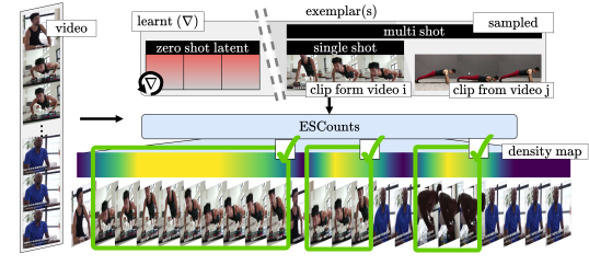
Taking inspiration from image-based approaches, we address Video Repetition Counting (VRC) using exemplars, for the first time. We differ from prior works that formulate VRC as classifying a preset number of repetitions [6, 16, 67], or consecutively detecting relevant parts of the repetition [15, 20, 30], such as the start/end. Instead, we argue that learning correspondences to reference exemplar(s) can provide a strong prior for discovering repetitions in videos. We propose Every-Shot Counts (ESCounts), a transformer-based encoder-decoder that encodes videos of varying lengths alongside exemplars and learns representations of general repeating motions, as shown in Figure 1. Similar to prior works [20, 30], we use the density map to regress the temporal location of each repetition. During training, we learn an exemplar latent representation, which we use for inference where no exemplars are available.
In summary, our contributions are as follows: (i) We introduce exemplar-based counting for VRC (ii) We propose an attention-based encoder-decoder that learns to correspond exemplars to a query video of varying length, and predict repetitions. (iii) We use a learnt latent for general motions in repetitions enabling our approach to predict the number of repetitions during inference without exemplars, (iv) We evaluate our approach on the three datasets commonly used for repetition counting in videos: RepNet [20], Countix [16], and UCFRep [65]. Our approach achieves a new state-of-the-art in every benchmark, even on Countix where the start-end times of repetitions are not annotated.
2 Related Works
We first review methods for the long-established task of object counting in images. We then review VRC methods for videos.
2.1 Object Counting in Images
Methods can be divided into class-specific and class-agnostic object counting.
Class-Specific Counting. These methods learn to count objects of singular classes or sets of categories e.g. people [56, 29], cars [19], wildlife [4]. A large portion of object-counting approaches [19, 56, 12, 40, 47] have relied on detecting target objects and counting their instances. Traditional methods have used hand-crafted feature descriptors to detect human heads [56] or head-shoulders [29] for crowd-counting. Other methods have used blobs [26], individual points [34], and object masks [13] for detecting and counting instances. Though object detection can be a preliminary step before counting, detection methods rely strongly on the performance of the object detector which can be less effective in densely crowded images [12]. A different set of methods has instead relied on regression, to either regress to the target count [12, 61] or estimate a density map [27, 41, 66].
Class-Agnostic Counting. Class-specific counting approaches are impractical for general setting, as prior knowledge of the object category is not available. Recent works [10, 3, 31, 48] have used one (or a few) exemplars as references to estimate a density map for unknown target classes. Exemplars for object counting were first introduced by Lu et al. [38]. Building on the property of image self-similarity, [38] proposed a convolutional matching network and cast counting as an image-matching problem, where exemplar patches from the same image are used to match against other patches within the image. Following up, Liu et al. [10] proposed a transformer-based feature interaction module. They used an encoder for the query image and a convolution-based encoder for the exemplar. The interaction module cross-attended information between the exemplar and image and used a convolutional decoder to regress the density map. Recent approaches have also fused text and visual embeddings [3], used contrastive learning across modalities [24], and generated exemplar prototypes using stable diffusion [62]. Inspired by these methods, we propose a fully-attention-based encoder-decoder that extends exemplar-based counting to VRC. Our approach is invariant to video lengths and can use both learnt or encoded exemplars.
2.2 Video Repetition Counting (VRC)
Compared to image-based counting, video repetition counting has been less explored. Early approaches have compressed motion into a one-dimensional signal and recovered the repetition structure from the signal’s period [2, 25, 37, 42]. The periodicity can then be counted by Fourier analysis [5, 7, 14, 43, 2, 25], peak detection [52], or wavelet analysis [46]. However, these methods are limited to uniformly periodic repetitions. For non-periodic repetitions, localisation frameworks [11, 36, 49, 33] have been adapted. Zhang et al. [65] proposed a context-aware scale-insensitive framework to count repetitions of varying scales and duration. Their method exhaustively searched for pairs of consecutive repetitions followed by a prediction refinement module. Recent methods [15, 16, 20] have also extended image self-similarity to the temporal dimension with temporal self-similarity matrices (TSM). TSM is constructed using pair-wise similarity of embeddings over temporal locations. RepNet [16] used a transformer-based period predictor. To count repetitions with varying speeds, Trans-RAC [20] modified TSM to use multi-scale sequence embeddings. For counting under poor lighting conditions, [67] used audio in tandem with video within a multi-modal framework. They selectively aggregated information from the two modalities using a reliability estimation module. Li et al. [30] also used multi-modal inputs with optical flow as an additional signal supporting RGB for detecting periodicity. Yao et al. [63] proposed a lightweight pose-based transformer model that used action-specific salient poses as anchors and matched them across the video. However, the requirement of salient pose labels for each action limits its generalisability to unseen repetitions.
The above methods do not utilise the correspondences discovered by exemplar repetitions. Thus, do not relate variations in the action’s performance, alongside other visual variations such as viewpoint and camera motion. To handle such cases, we propose using action exemplars as references for VRC. Exemplars have previously been used in videos for action recognition tasks [17, 23, 59, 58]. [58] used silhouette/pose exemplars for classifying action sequences into predefined action categories using a Bayes classifier. [59] converted training videos to visual vocabulary and used the most discriminative visual words as exemplars for detecting actions. These methods are limited to a predefined set of classes and will be ineffective for class-agnostic tasks such as repetition counting. To our knowledge, we are the first to use exemplars for repetition counting in videos.
3 Every Shot Counts (ESCounts) Model
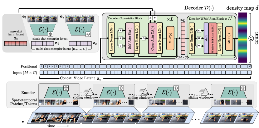
In this section, we introduce our ESCounts model (overviewed in Figure 2). We formally define encoding variable length videos alongside our model’s output, in Section 3.1. We then introduce the attention-based decoder that corresponds the input video to exemplars in Section 3.2. Predictions over temporally shifted inputs are combined for a final prediction, detailed in Section 3.3.
3.1 Input Encoding and Output Prediction
We denote the full video as of varying length and a fixed spatial resolution. Segment containing a single instance of the repeating action we wish to count, is selected as an exemplar. Exemplars are defined based on provided start, end labels of every repetition in the video111For datasets where the start/end times are not available, pseudo-labels are used instead by uniformly dividing the video given the ground truth count.. During training, we select one or more exemplar shots . Each training sample is thus a combination of the query video and a set of exemplars .
We tokenise and encode the video from its original size into spatiotemporal latents . Encoder is applied over a fixed-size sliding window, to account for the video’s variable length. The encoded video is represented by of spatiotemporal resolution with channels. We note that is not a fixed number, as it depends on the video’s length . We add sinusoidal positional encoding to account for the relative order of these spatiotemporal latents while accommodating the variable video length.
During training, we select exemplars from either the same video or another video containing the same action label; e.g. given a video containing push-up actions, we can sample exemplars from other videos showcasing the same action within the training set. We define a probability of sampling the exemplar from a different video; i.e. implies exemplars are only sampled from the same video, whereas for exemplars are always sampled from another video222We ablate in our experiments.. In training, exemplars are sampled randomly from the labelled repetitions of the video. We use to encode latent representations from each exemplar . We use the same encoder for encoding and to allow correspondence.
We construct the ground truth density map from the labelled repetitions in the video as a 1-dimensional vector. To match the downsampled temporal resolution of our input video , we also temporally downsample the ground-truth labels. The density map takes low values () at temporal locations without repetitions in the video, and high within repetitions. We use a normal distribution centred around each repetition with , where and are the start and end times of each repetition .
| (1) |
Note that the sum of the density map matches the ground truth count, i.e. where is the ground truth count for the video.
3.2 Latent Exemplar Correspondence
Given both the encoded video and exemplars latents, we use an attention-based decoder to attend to every repetition in the video that matches the encoded exemplar. Decoder takes the encoded video as input and predicts the location of every repetition in the video. The decoder outputs a 1-dimensional predicted density map of length corresponding to the occurrences of the repeating action given the exemplars.
Cross-attention Blocks. We explore the similarity between representations of exemplars and the query video to predict the corresponding locations of repetitions that match the exemplar. Thus, inspired by [10], we use cross-attention to relate exemplar and video latents. We define cross-attention blocks. Each block initially self-attends the video latents with multi-head self-attention. We note that for the first layer, . Then we relate exemplar and video information by cross-attending video and exemplar latents. The block’s initial self-attention operation is formulated as:
| (2) |
where is layer normalisation.
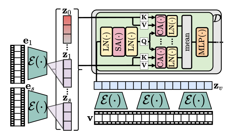
Repetitions can vary by viewing angles, performance, or duration. We thus wish to enable the inclusion of a varying number of exemplars for counting a repeating action, as shown in Figure 3. Given a selected number of exemplar shots , we apply CA in parallel with used as a shared query and each of the exemplars used as keys and values enabling the fusion of repetition-relevant information. As the latents of the video are used as queries , spatiotemporal resolution is maintained. Outputs are then averaged:
| (3) |
where is the set of exemplars selected and is the latent for the exemplar.
We also want to learn representations for repeating motions to estimate repetitions without explicitly providing exemplars. We thus define a learnable latent to cross-attend . At each training iteration, we select exemplars from and perform CA with or . At inference, we use .
We use a multi-layer perceptron MLP on the exemplar-fused latents .
| (4) |
The cross-attention blocks’ output is defined as .
Window Self-attention Blocks. We explore the spatio-temporal inductive bias within the self-attention blocks. Each latent thus attends locally, to its spatio-temporal neighbouring tokens, over window self-attention [35] layers. We denote :
| (5) |
where WSA is window self-attention. Note that following [35] windows are shifted at each layer to account for connections across different windows.
The output of the window self-attention blocks is of size . In turn, encodes repetition-relevant features over space and time. Thus, we use to predict density map for the occurrences of the target repeating action over time. We use a fully connected layer to project the latent to a 1-channel vector, i.e. MLP: . We then pool the spatial resolution resulting to predicted density map .
Training Objective. Given ground-truth and the predicted density maps, we train to regress the Mean Square Error between and , and following [67], the Mean Absolute Error between ground truth counts and the predicted counts obtained by linearly summing the density map
| (6) |
At inference, we use the predicted count .
3.3 Time-Shift Augmentations
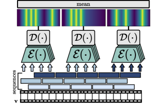
The predicted density map results from encoding a video with , over non-overlapping sliding windows. However, as each window is of fixed temporal resolution, repetitions may span over multiple windows. Thus, we include time-shifting augmentations in which the start time of the encoded video is adjusted to allow for different spatiotemporal tokens. We train with augmentations of the start time whilst at inference, we use an ensemble of time-shift augmentations for a more robust estimation. We use multiple overlapping sequences as shown in Figure 4 and combine the predicted density maps over shifted start/end positions. We obtain the final predicted density map by temporally aligning and averaging the predictions.
| (7) |
where is the shifting for each .
4 Experiments
We overview the used datasets, implementation details, and evaluation metrics in Sec. 4.1. We include quantitative and qualitative comparisons to state-of-the-art methods in Sec. 4.2. We ablate over different ESCounts settings in Sec. 4.3. We demonstrate ESCounts’ ability to utilise exemplars at inference, in Sec. 4.4.
4.1 Experimental Setup
Datasets. We evaluate our method on a diverse set of VRC datasets.
RepCount [20] contains videos of workout activities of varying repetition durations and appearances. Annotations include count labels alongside start and end timestamps per repetition. We use the publicly available Part-A of the dataset with , , and videos for train, val, and test respectively. We tune the hyperparameters on the val set and report our results on the test set.
Countix [16] is a subset of Kinetics [9] containing videos of repetitive actions and their associated counts. It is the largest VRC dataset with , , and videos for train, val, and test respectively. Count annotations are provided per video, without individual repetition start-end times. We use pseudo-repetition annotations by dividing the videos into uniform segments based on the ground truth count, as Countix does not have many pauses or interruptions between counts. We use the pseudo-labels for estimating the density maps, without additional annotations, to compare directly to other methods.
UCFRep [65] is a subset of UCF-101 [51] consisting of 420 videos for train and 106 videos for val from 23 categories. Following [65, 30], we report our results on the val split as no test set is available. Like RepCount, it includes annotations of start and end timestamps for each repetition.
Implementation Details. Unless specified otherwise, we use VideoMAE-VIT-B [55] as our encoder with weights pre-trained on Kinetics-400 [9]. We sample frames from variable-length videos every 4 frames using a sliding window of frames. At each window, our encoder’s input is of size, and the output is , resulting in spatiotemporal tokens. We use channels333when encoders have a different output, we add a fully connected layer to map to . The input to the decoder is of variable length , where is the total number of frames in the video at raw framerate. Exemplars are sampled uniformly with frames between the start and end of a repetition.
The encoder is frozen with only the decoder and the zero-shot latent being trained. We use and . We ablate and in the supplementary material. We train our model on a single Tesla V100 for 300 epochs with a batch size of 1, to deal with variable-length videos, and accumulate gradients over 8 batches. We use an initial learning rate of and decay it every epochs by , and a weight decay of . For each training instance, we randomly set the number of exemplars and sample exemplars. We set the chance of sampling exemplars from a different video to .
At inference, we only use the learnt latent to predict repetition counts. We aggregate predictions over sequences.
Evaluation Metrics. Following previous repetition counting works [20, 16, 67], we use Mean Absolute Error (MAE) and Off-By-One accuracy (OBO) as evaluation metrics, calculated as Eqs. 8 and 9 respectively. Inspired by image counting methods [10, 3], we introduce Root-Mean-Square-Error (RMSE) in Eq. 10 for VRC providing a more robust metric for diverse counts compared to MAE’s bias towards small counts. With continuous improvements in repetition counting methods, we also report the off-by-zero accuracy (OBZ) in Eq. 11 as a tighter metric than the corresponding OBO for precise counts.
| (8) |
| (9) |
| (10) |
| (11) |
where , are the ground-truth and predicted counts for -th video in test set . is the indicator function.
4.2 Comparison with State-of-the-art
In Tab. 2, we compare our method, ESCounts, to prior methods on the three datasets. We also provide results on the same backbone as the best-performing method on each dataset, for fair and direct comparison to previous works.
| Method | Encoder | RMSE | MAE | OBZ | OBO |
| Levy & Wolf [28] | RX3D101 | - | 0.286 | - | 0.680 |
| RepNet [16] | R2D50 | - | 0.998 | - | 0.009 |
| Context (F) [65] | RX3D101 | 5.761∗ | 0.653∗ | 0.143∗ | 0.372∗ |
| TransRAC [20] | VSwinT | - | 0.640 | - | 0.324 |
| MFL[30] | RX3D101 | - | 0.388 | - | 0.510 |
| ESCounts | RX3D101 | 2.004 | 0.247 | 0.343 | 0.731 |
| ESCounts | VMAE | 0.216 | 0.381 | 0.704 | |
| Context [65] | RX3D101 | 2.165∗ | 0.147 | ∗ | 0.790 |
| Sight & Sound [67] | R(2+1)D18 | - | - |
Tab. 2 - RepCount. We demonstrate that our ESCounts model outperforms recent methods [20, 30] with the same Swin Tiny (VSwinT) [35] encoder, by in MAE and in OBO. Our approach also improves upon [30] which uses optical flow and video in tandem, by margins of in MAE and in OBO. The largest improvements are observed with VideoMAE (VMAE) surpassing [20] on the introduced OBZ by and reducing RMSE by .
Tab. 2 - Countix. Compared to the state-of-the-art [16, 67] our ESCounts consistently outperforms other models with the same R(2+1)D18 encoder. Our video-only model surpasses the audio-visual model in [67] by OBO. Further improvements on the RMSE, MAE, and OBZ are observed with VMAE.
Tab. 2 - UCFRep. Across approaches with frozen encoders ESCounts improve the top-performing [30] by OBO and MAE. Our method does not outperform [67, 65] that fine-tune their encoders on the training set of UCFRep which is advantageous given the dataset’s size as also noted in [30]. We showcase this with Context (F) trained from the publicly available code of [65] with a frozen encoder and result in a significant drop in performance with +0.51 MAE and -0.42 OBO. Despite this, we achieve strong results.
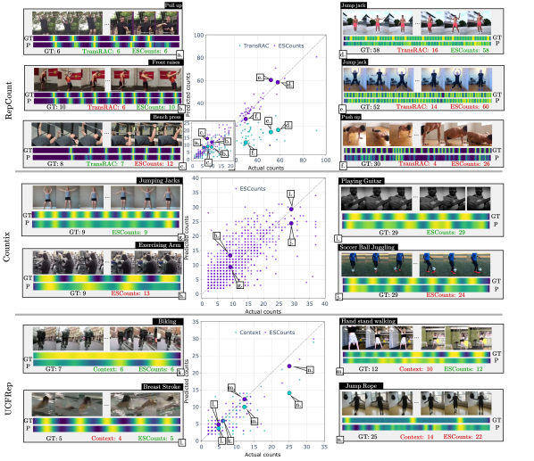
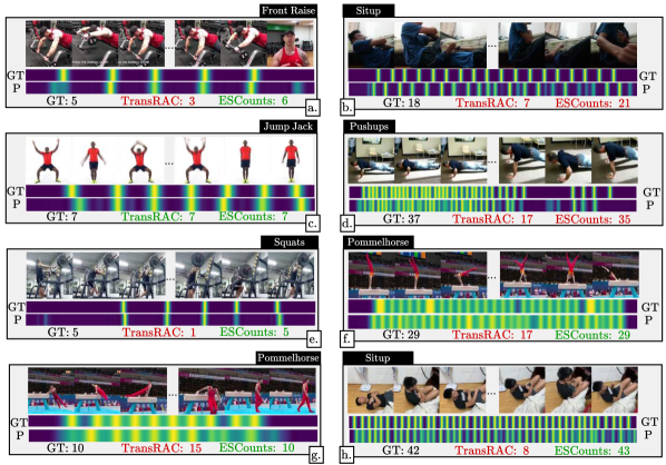
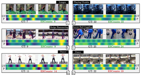
Qualitative Results. In Fig. 5 we visualise predicted to ground truth counts. For RepCount and UCFRep, we select [20] and [65] as respective baselines and use their publicly available checkpoints444[30] was not used as a baseline as the code is not public. The publicly available checkpoints on Countix obtained lower results than originally reported.. ESCounts accurately predicts the number of repetitions for a wide range of counts, with most predictions being close to the diagonal. Though predictions from both the baseline and ESCounts are close to the ground truth in low counts, they significantly diverge in high counts. We additionally visualise specific examples with sample frames from these videos. ESCounts is robust to the magnitude of counts, with accurate predictions over low count (a,b,g,k,l) and high count (d,i,m) examples. In cases of over- and under-predictions; e.g. (c,e,f,h,j,n) ESCounts predictions remain closer to actual counts. As shown by the density maps, ESCounts can also localise the repetitions. For Countix, because the model was trained on pseudo labels, even though ESCounts can predict accurate counts, it struggles to localise the repetitions at times. We further investigate the localisation capabilities in the supplementary.
Cross-dataset Generalisation. Following prior works [20, 30], we also test the generalisation capabilities of our method. We use our model trained on RepCount and evaluate it on the test sets of UCFRep and Countix. As shown in Tab. 2, our method achieves the best results surpassing [30] by in MAE and in OBO in UCFRep. We also explore cross-dataset generalisation for Countix, and select [20] as a baseline with the public checkpoint. We outperform [20] by significant margins across metrics, showcasing the strong ability of ESCounts to generalise across datasets.
4.3 Ablation Studies
In this section, we conduct ablation studies on RepCount [20] using VMAE as the encoder. We study the impact of exemplars by replacing cross- with self-attention and vary the number of exemplars used during training. We evaluate the sensitivity of our method to the exemplar sampling probability . We ablate in density map estimation and analyse the impact of time-shift augmentations and our loss function’s components.
| RMSE | MAE | OBZ | OBO | |
| SA-only | 5.654 | 0.273 | 0.147 | 0.470 |
| ESCounts |
| RMSE | MAE | OBZ | OBO | |
| 4.962 | 0.240 | 0.223 | 0.519 | |
| 4.633 | 0.228 | 0.236 | 0.546 | |
| 4.601 | 0.226 | 0.239 | 0.550 | |
| Diff | same | ||||
|---|---|---|---|---|---|
| video | class | RMSE | MAE | OBZ | OBO |
| ✗ | - | 4.701 | 0.224 | 0.226 | 0.521 |
| ✔ | ✗ | 5.553 | 0.270 | 0.165 | 0.464 |
| ✔ | ✔ |
| RMSE | MAE | OBZ | OBO | |
| 4.919 | 0.240 | 0.205 | 0.545 | |
| 4.654 | 0.221 | 0.236 | 0.550 | |
| 4.561 | 0.218 | 0.240 | 0.558 | |
| 4.735 | 0.230 | 0.223 | 0.553 | |
| 5.012 | 0.245 | 0.218 | 0.532 |
| RMSE | MAE | OBZ | OBO | |
| Variable | 6.152 | 0.301 | 0.165 | 0.457 |
| 0 | 5.145 | 0.241 | 0.206 | 0.510 |
| 0.25 | 4.871 | 0.226 | 0.228 | 0.542 |
| 0.50 | ||||
| 0.75 | 4.683 | 0.218 | 0.240 | 0.556 |
| 1.00 | 4.732 | 0.223 | 0.238 | 0.552 |
| RMSE | MAE | OBZ | OBO | |
| 1 | 4.592 | 0.221 | 0.235 | 0.552 |
| 2 | 4.493 | 0.217 | 0.242 | 0.556 |
| 3 | 4.471 | 0.213 | 0.243 | 0.561 |
| 4 |
| Obj | RMSE | MAE | OBZ | OBO |
|---|---|---|---|---|
| MSE | 5.109 | 0.273 | 0.215 | 0.532 |
| MAE |
Do exemplars help in training? We study the impact of using exemplars for training by directly replacing the cross-attention decoder blocks with self-attention. As seen in Tab. 3, using self-attention (SA-only) performs significantly worse than our proposed ESCounts. Cross-attending exemplars decrease the RMSE/MAE by and whilst improving OBZ and OBO by and , thus emphasising the benefits of exemplar-based VRC.
How many exemplars to sample? Since we use a varying number of exemplars whilst training, we also experiment by varying from in Tab. 3. In we train only with the learnt zero-shot latent. Training with provides the best zero-shot scores in inference. We believe training with a larger and more diverse set of exemplars helps the model to learn a general zero-shot token that can capture general information about repetitions. Due to memory constraints, we could not train with more than 2 exemplars.
How to sample exemplars? We analyse the impact of sampling exemplars from other videos, from the same or a different action class. As expected, Tab. 3 shows that keeping the same action category for both exemplars and query video performs the best, as ensuring the same action semantics between exemplars and query video helps to learn their correspondence. In this table, we used sampling probability .
We vary the sampling probability from other videos of the same underlying action in Tab. 3. For exemplars are sampled exclusively from the query video, whilst for exemplars are sampled solely from other videos of the same class. The best performance was observed with , showcasing sampling from the same video to be critical for learning.
#
What’s the impact of time-shift augmentations? As predictions are aggregated over density maps by time-shifting the video input. As shown in Tab. 3, having shifted start/end positions provides the best results. However, results are strong even without test-time augmentations in .
What should be the density map variance? Density maps are constructed as vectors with normal distributions over repetition starts/ends timestamps. Reducing increases the sharpness, resulting in a single delta function for . We ablate over different in Tab. 3. Denser and successive repetitions can benefit from sharper peaks of small and sparser repetitions of larger durations can benefit from large . We also ablate using variable that changes with the duration of repetition segments. Having provides the best results with a balance between sharpness and covering the duration of repetitions.
How helpful is the MAE for the objective? We analyse ESCounts’ performance with and without the MAE loss from [67] in Tab. 3. The combined objective helps performance for diverse counts across all metrics.
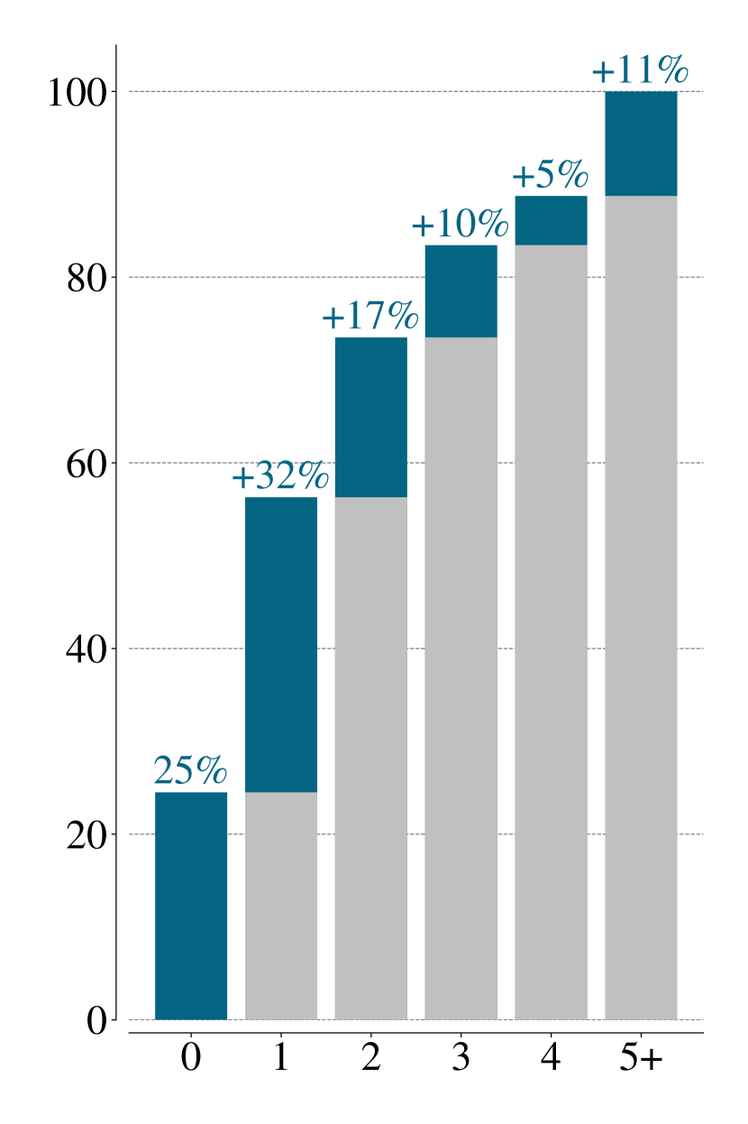
How close are predictions to the ground truth?. We further relax the off-by metrics to Off-By-N in Figure 6(a) to visualise the proximity of predictions to the ground truth. Overall, 84% of predictions are within of the actual count.
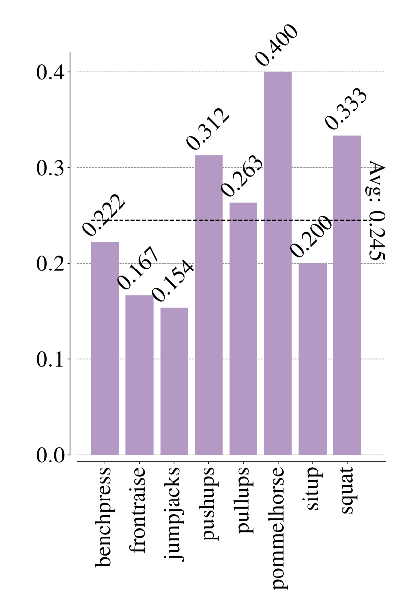
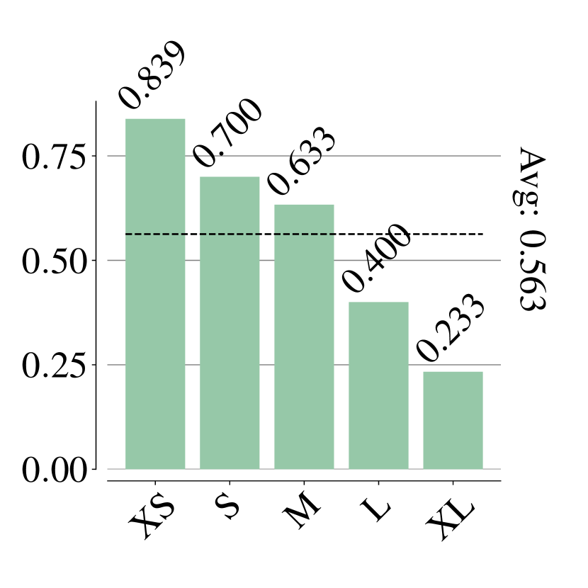
What is the performance per action category?. In Figure 6(b), we plot the OBZ per action class. ESCounts performs fairly uniformly across all classes with the best performing categories being pommelhourse and squat.
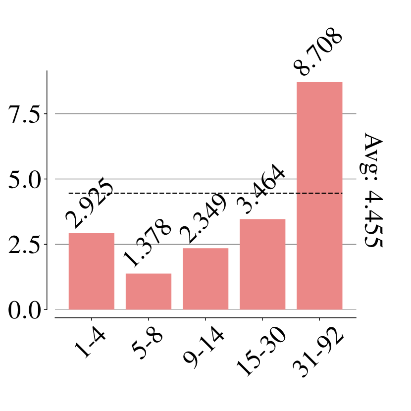
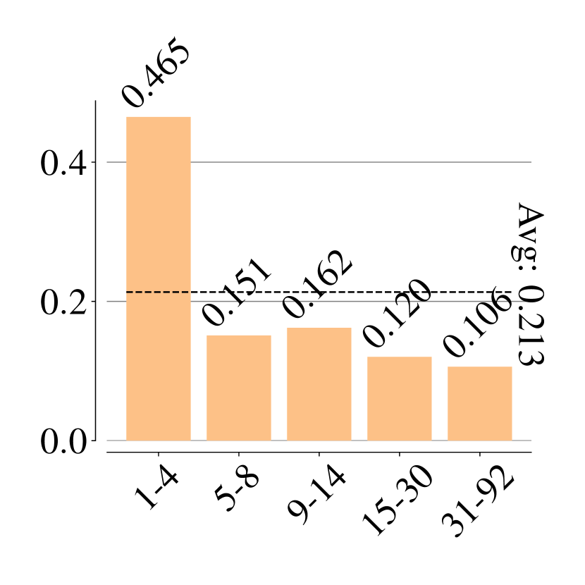
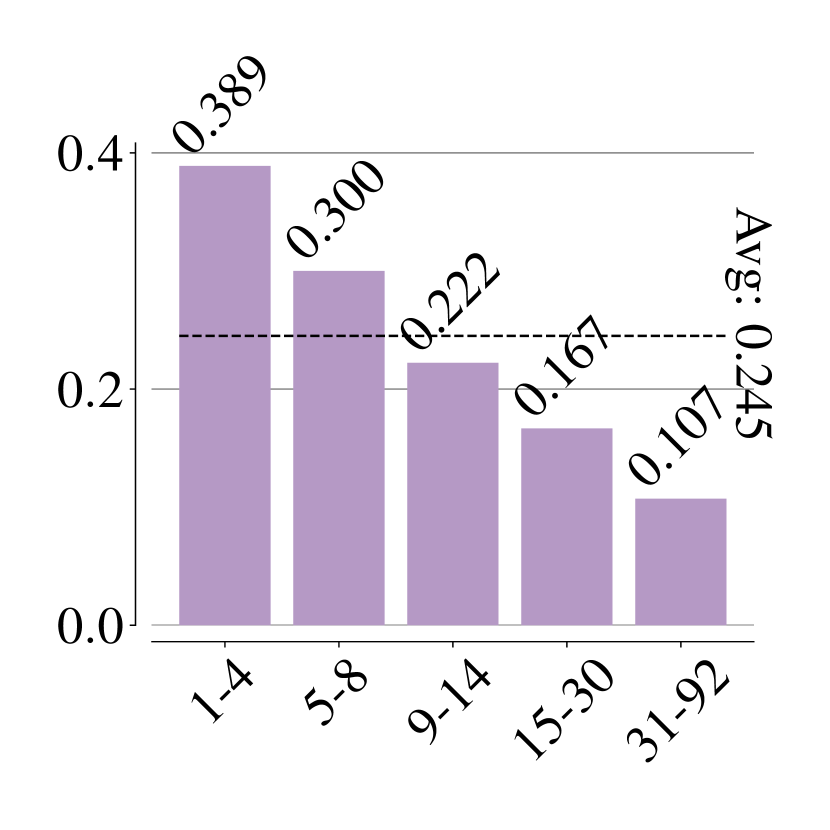
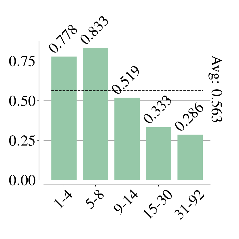
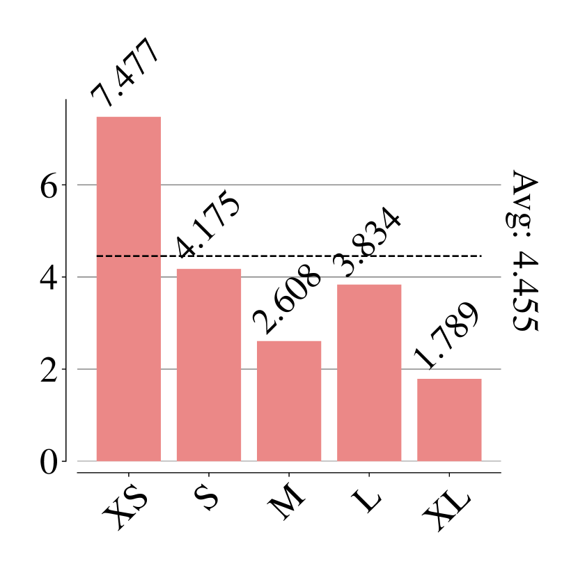
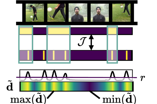
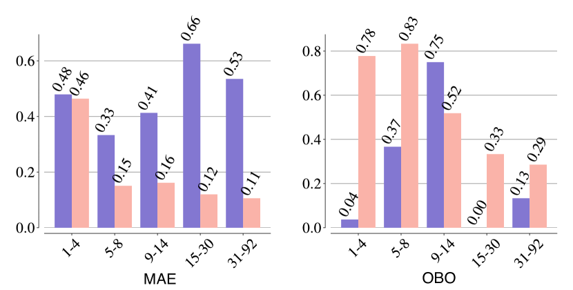
How does performance differ across counts, repetition lengths, and video durations? Up to this point, we have focused on the performance across all videos regardless of individual attributes. We now consider the sensitivity of ESCounts across equally sized groups based on the number of repetitions, average repetition length, and video duration.
We report all metrics over groups of counts in Figs. 6(c), 6(d), 6(e) and 6(f). As expected, our method performs best in groups of smaller counts with higher counts being more challenging to predict precisely.
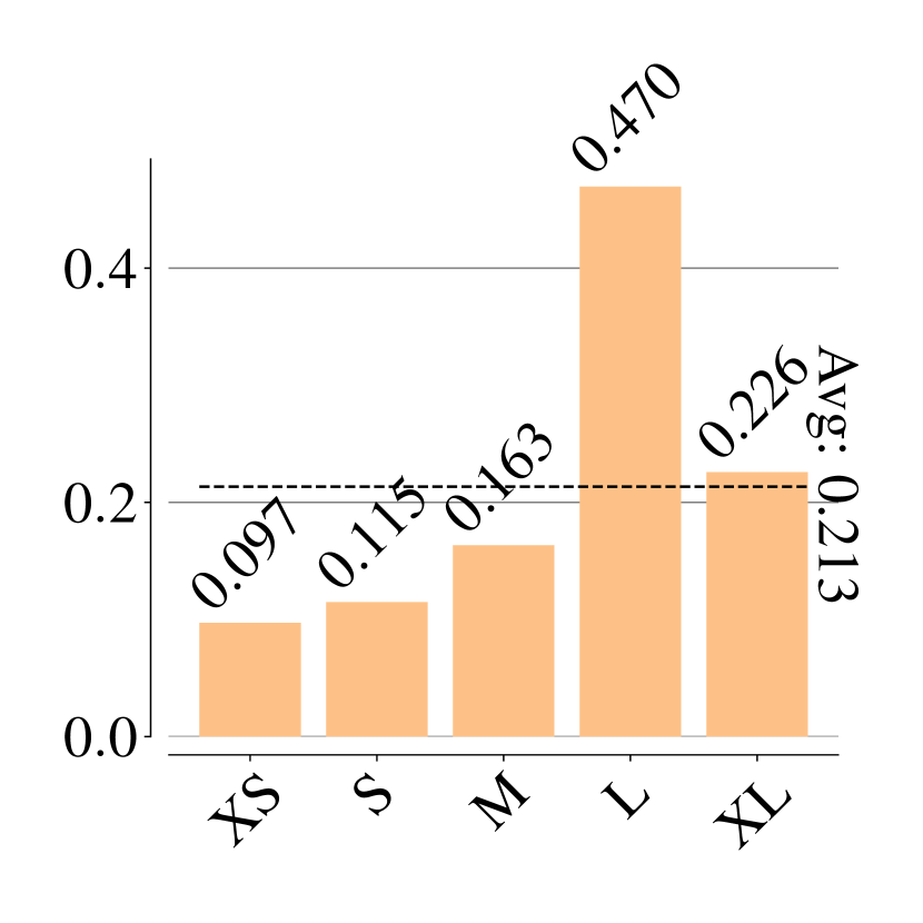
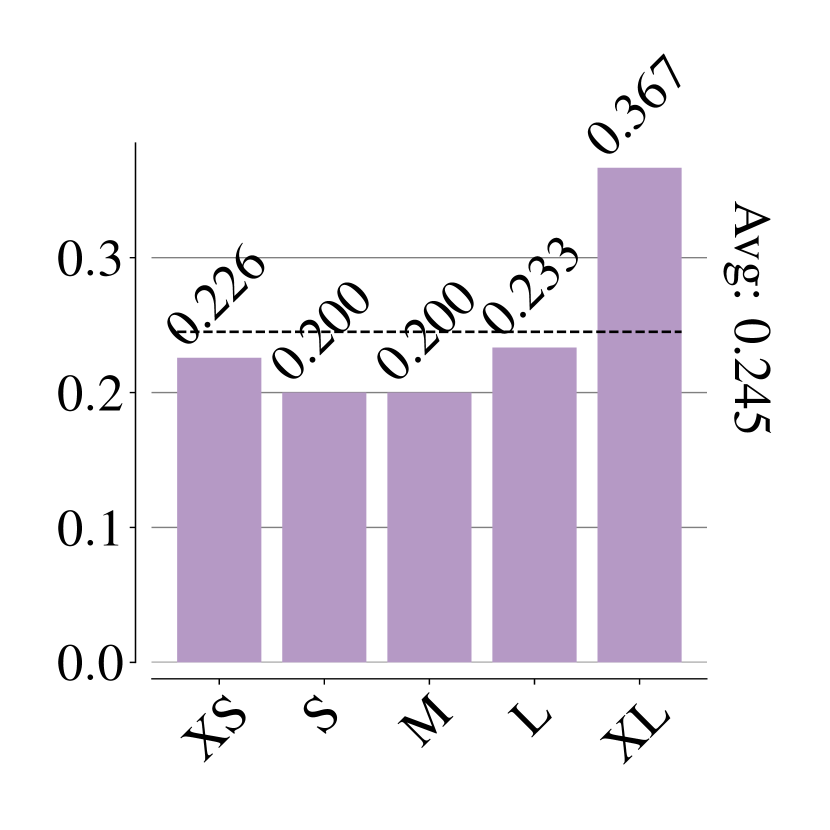
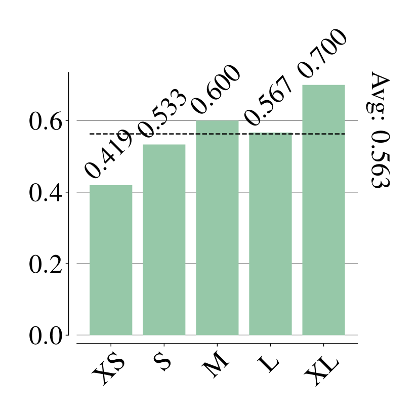
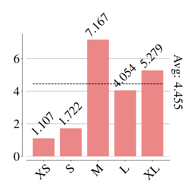
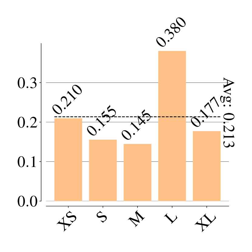
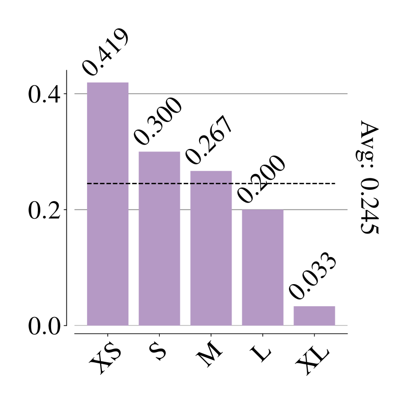
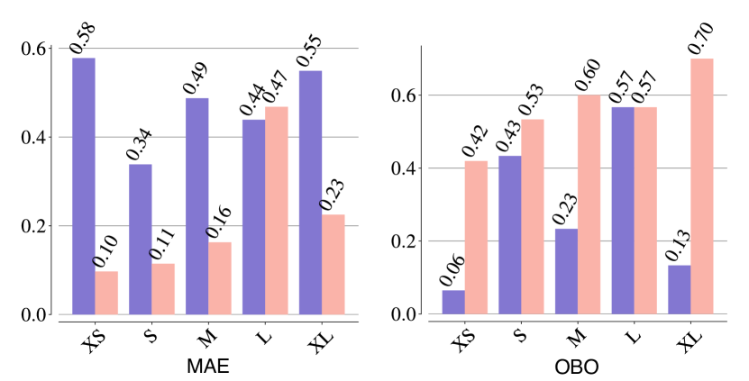
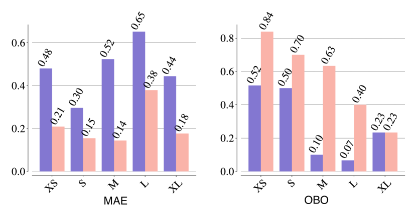
In Figs. 6(g), 6(h), 6(i) and 6(j) we report VRC metrics with results grouped by average video repetition duration. These are grouped, into equal sized bins, to XS=(0-0.96)s, S=(0.96-1.53)s, M=(1.53-2.29)s, L=(2.29-3.09)s, XL=(>3.09)s. Predicting density maps is more challenging for short repetitions. However, ESCounts can still correctly predict counts across repetition lengths as shown by Figures 6(i) and 6(j). We also group videos by duration into XS=(8.0-11.0)s, S=(11.0, 26.0)s, M=(26.0, 33.9)s, L=(33.9-45.9)s and XL=(45.9-68.0)s. From Figures 6(k), 6(l), 6(m) and 6(n), counting repetitions from longer videos is more challenging.
| RepCount | UCFRep | |||||||||
| Shots | Same video | RMSE | MAE | OBZ | OBO | RMSE | MAE | OBZ | OBO | |
| 0 | N/A | 4.455 | 0.213 | 0.245 | 0.563 | 1.972 | 0.216 | 0.381 | 0.704 | |
| 1 | ✗ | 4.432 | 0.207 | 0.251 | 0.563 | 1.912 | 0.211 | 0.388 | 0.712 | |
| ✔ | 4.369 | 0.210 | 0.247 | 0.589 | 1.890 | 0.203 | 0.400 | 0.714 | ||
| 2 | ✗ | 4.384 | 0.251 | 0.572 | 1.885 | 0.208 | 0.391 | 0.720 | ||
| ✔ | 4.360 | 0.209 | 0.247 | 0.592 | 1.857 | 0.199 | 0.419 | 0.718 | ||
| 3 | ✗ | 4.381 | 0.207 | 0.579 | 1.878 | 0.207 | 0.399 | |||
| ✔ | 0.250 | 0.723 | ||||||||
4.4 Inference with More Shots
up to this point, only the learnt zero-shot latent was used for inference.
Prior works in object counting [10, 38] have reported results using exemplars (i.e. object crops) in inference. While this is not comparable to other works in VRC, we can assess our method’s ability to utilise exemplars during inference in Tab. 4. Video exemplars steadily improve performance as the number of exemplars increases. As our model cross-attends exemplars in parallel, we can train with exemplars, and use exemplars during inference. We show comparable results when sampling exemplars from the test video vs exemplars from the training set videos showcasing the same action category. Combined with a classifier, one can envisage an approach that classifies the action then sources exemplars from the training set to assist counting during inference.
5 Conclusion
We have proposed to utilise exemplars for video repetition counting. We introduce Every Shot Counts (ESCounts), an attention-based encoder-decoder that learns to correspond exemplar repetitions across a full video. We define a learnable zero-shot latent that learns representations of generic repetitions, to use during inference. Extensive evaluation on RepCount, Countix, and UCFRep demonstrates the merits of ESCounts achieving state-of-the-art results on the traditional MAE and OBO metrics and the newly introduced RMSE and OBZ. Further analysis showed that the exemplars do not need to be from the same video as long as they belong to the same action class. The diversity of these exemplars is an aspect for future exploration.
Acknowledgements
This work uses publicly available datasets and annotations to produce all results and ablations. Research is supported by EPSRC UMPIRE (EP/T004991/1). S. Sinha is supported by EPSRC DTP (Doctoral Training Program) studentship.
References
- [1] Alayrac, J.B., Donahue, J., Luc, P., Miech, A., Barr, I., Hasson, Y., Lenc, K., Mensch, A., Millican, K., Reynolds, M., et al.: Flamingo: a Visual Language Model for Few-Shot Learning. Advances in Neural Information Processing Systems (NeurIPS) pp. 23716–23736 (2022)
- [2] Albu, A.B., Bergevin, R., Quirion, S.: Generic Temporal Segmentation of Cyclic Human Motion. Pattern Recognition 41(1), 6–21 (2008)
- [3] Amini-Naieni, N., Amini-Naieni, K., Han, T., Zisserman, A.: Open-world Text-specified Object Counting. In: British Machine Vision Conference (BMVC) (2023)
- [4] Arteta, C., Lempitsky, V., Zisserman, A.: Counting in the Wild. In: European Conference on Computer Vision (ECCV). pp. 483–498 (2016)
- [5] Azy, O., Ahuja, N.: Segmentation of Periodically Moving Objects. In: International Conference on Pattern Recognition (ICPR). pp. 1–4 (2008)
- [6] Bacharidis, K., Argyros, A.: Repetition-aware Image Sequence Sampling for Recognizing Repetitive Human Actions. In: International Conference on Computer Vision Workshops (ICCVw). pp. 1878–1887 (2023)
- [7] Briassouli, A., Ahuja, N.: Extraction and Analysis of Multiple Periodic Motions in Video Sequences. IEEE Transactions on Pattern Analysis and Machine Intelligence (TPAMI) 29(7), 1244–1261 (2007)
- [8] Caba Heilbron, F., Escorcia, V., Ghanem, B., Carlos Niebles, J.: ActivityNet: A Large-Scale Video Benchmark for Human Activity Understanding. In: Conference on Computer Vision and Pattern Recognition (CVPR). pp. 961–970 (2015)
- [9] Carreira, J., Zisserman, A.: Quo Vadis, Action Recognition? A New Model and the Kinetics Dataset. In: Conference on Computer Vision and Pattern Recognition (CVPR). pp. 6299–6308 (2017)
- [10] Chang, L., Yujie, Z., Andrew, Z., Weidi, X.: CounTR: Transformer-based Generalised Visual Counting. In: British Machine Vision Conference (BMVC) (2022)
- [11] Chao, Y.W., Vijayanarasimhan, S., Seybold, B., Ross, D.A., Deng, J., Sukthankar, R.: Rethinking the Faster R-CNN Architecture for Temporal Action Localization. In: Conference on Computer Vision and Pattern Recognition (CVPR). pp. 1130–1139 (2018)
- [12] Chattopadhyay, P., Vedantam, R., Selvaraju, R.R., Batra, D., Parikh, D.: Counting Everyday Objects in Everyday Scenes. In: Conference on Computer Vision and Pattern Recognition (CVPR). pp. 1135–1144 (2017)
- [13] Cholakkal, H., Sun, G., Khan, F.S., Shao, L.: Object Counting and Instance Segmentation with Image-level Supervision. In: Conference on Computer Vision and Pattern Recognition (CVPR). pp. 12397–12405 (2019)
- [14] Cutler, R., Davis, L.S.: Robust Real-Time Periodic Motion Detection, Analysis, and Applications. IEEE Transactions on Pattern Analysis and Machine Intelligence (TPAMI) 22(8), 781–796 (2000)
- [15] Destro, M., Gygli, M.: CycleCL: Self-supervised Learning for Periodic Videos. In: Winter Conference on Applications of Computer Vision (WACV). pp. 2861–2870 (2024)
- [16] Dwibedi, D., Aytar, Y., Tompson, J., Sermanet, P., Zisserman, A.: Counting Out Time: Class Agnostic Video Repetition Counting in the Wild. In: Conference on Computer Vision and Pattern Recognition (CVPR). pp. 10387–10396 (2020)
- [17] Gaidon, A., Harchaoui, Z., Schmid, C.: Temporal Localization of Actions with Actoms. IEEE Transactions on Pattern Analysis and Machine Intelligence (TPAMI) 35(11), 2782–2795 (2013)
- [18] Gu, C., Sun, C., Ross, D.A., Vondrick, C., Pantofaru, C., Li, Y., Vijayanarasimhan, S., Toderici, G., Ricco, S., Sukthankar, R., et al.: AVA: A Video Dataset of Spatio-Temporally Localized Atomic Visual Actions. In: Conference on Computer Vision and Pattern Recognition (CVPR). pp. 6047–6056 (2018)
- [19] Hsieh, M.R., Lin, Y.L., Hsu, W.H.: Drone-based Object Counting by Spatially Regularized Regional Proposal Network. In: International Conference on Computer Vision (ICCV). pp. 4145–4153 (2017)
- [20] Hu, H., Dong, S., Zhao, Y., Lian, D., Li, Z., Gao, S.: TransRAC: Encoding Multi-scale Temporal Correlation with Transformers for Repetitive Action Counting. In: Conference on Computer Vision and Pattern Recognition (CVPR). pp. 19013–19022 (2022)
- [21] Huang, J., Li, Y., Feng, J., Wu, X., Sun, X., Ji, R.: Clover: Towards A Unified Video-Language Alignment and Fusion Model. In: Conference on Computer Vision and Pattern Recognition (CVPR). pp. 14856–14866 (2023)
- [22] Idrees, H., Zamir, A.R., Jiang, Y.G., Gorban, A., Laptev, I., Sukthankar, R., Shah, M.: The thumos challenge on action recognition for videos “in the wild". Computer Vision and Image Understanding 155, 1–23 (2017)
- [23] Jain, M., Ghodrati, A., Snoek, C.G.: ActionBytes: Learning From Trimmed Videos to Localize Actions. In: Conference on Computer Vision and Pattern Recognition (CVPR). pp. 1171–1180 (2020)
- [24] Jiang, R., Liu, L., Chen, C.: CLIP-Count: Towards Text-Guided Zero-Shot Object Counting. In: ACM International Conference on Multimedia. p. 4535–4545 (2023)
- [25] Laptev, I., Belongie, S.J., Pérez, P., Wills, J.: Periodic Motion Detection and Segmentation via Approximate Sequence Alignment. In: International Conference on Computer Vision (ICCV). pp. 816–823 (2005)
- [26] Laradji, I.H., Rostamzadeh, N., Pinheiro, P.O., Vazquez, D., Schmidt, M.: Where are the Blobs: Counting by Localization with Point Supervision. In: European Conference on Computer Vision (ECCV). pp. 547–562 (2018)
- [27] Lempitsky, V., Zisserman, A.: Learning to Count Objects in Images. Advances in Neural Information Processing Systems (NeurIPS) (2010)
- [28] Levy, O., Wolf, L.: Live Repetition Counting. In: International Conference on Computer Vision (ICCV). pp. 3020–3028 (2015)
- [29] Li, M., Zhang, Z., Huang, K., Tan, T.: Estimating the Number of People in Crowded Scenes by MID Based Foreground Segmentation and Head-shoulder Detection. In: International Conference on Pattern Recognition (ICPR). pp. 1–4 (2008)
- [30] Li, X., Xu, H.: Repetitive Action Counting With Motion Feature Learning. In: Winter Conference on Applications of Computer Vision (WACV). pp. 6499–6508 (2024)
- [31] Lin, H., Hong, X., Wang, Y.: Object Counting: You Only Need to Look at One. arXiv preprint arXiv:2112.05993 (2021)
- [32] Lin, K.Q., Zhang, P., Chen, J., Pramanick, S., Gao, D., Wang, A.J., Yan, R., Shou, M.Z.: UniVTG: Towards Unified Video-Language Temporal Grounding. In: International Conference on Computer Vision (ICCV). pp. 2794–2804 (2023)
- [33] Lin, T., Zhao, X., Su, H., Wang, C., Yang, M.: BSN: Boundary Sensitive Network for Temporal Action Proposal Generation. In: European conference on computer vision (ECCV). pp. 3–19 (2018)
- [34] Liu, C., Weng, X., Mu, Y.: Recurrent Attentive Zooming for Joint Crowd Counting and Precise Localization. In: Conference on Computer Vision and Pattern Recognition (CVPR). pp. 1217–1226 (2019)
- [35] Liu, Z., Ning, J., Cao, Y., Wei, Y., Zhang, Z., Lin, S., Hu, H.: Video Swin Transformer. In: Conference on Computer Vision and Pattern Recognition (CVPR). pp. 3202–3211 (2022)
- [36] Long, F., Yao, T., Qiu, Z., Tian, X., Luo, J., Mei, T.: Gaussian Temporal Awareness Networks for Action Localization. In: Conference on Computer Vision and Pattern Recognition (CVPR). pp. 344–353 (2019)
- [37] Lu, C., Ferrier, N.J.: Repetitive Motion Analysis: Segmentation and Event Classification. IEEE Transactions on Pattern Analysis and Machine Intelligence (TPAMI) 26(2), 258–263 (2004)
- [38] Lu, E., Xie, W., Zisserman, A.: Class-agnostic Counting. In: Asian Conference on Computer Vision (ACCV). pp. 669–684 (2019)
- [39] Mangalam, K., Akshulakov, R., Malik, J.: EgoSchema: A Diagnostic Benchmark for Very Long-form Video Language Understanding. Advances in Neural Information Processing Systems (NeurIPS) (2023)
- [40] Noroozi, M., Pirsiavash, H., Favaro, P.: Representation Learning by Learning to Count. In: International Conference on Computer Vision (ICCV). pp. 5898–5906 (2017)
- [41] Oñoro-Rubio, D., López-Sastre, R.J.: Towards perspective-free object counting with deep learning. In: European Conference on Computer Vision (ECCV). pp. 615–629 (2016)
- [42] Panagiotakis, C., Karvounas, G., Argyros, A.: Unsupervised Detection of Periodic Segments in Videos. In: International Conference on Image Processing (ICIP). pp. 923–927 (2018)
- [43] Pogalin, E., Smeulders, A.W., Thean, A.H.: Visual Quasi-Periodicity. In: Conference on Computer Vision and Pattern Recognition (CVPR). pp. 1–8 (2008)
- [44] Pramanick, S., Song, Y., Nag, S., Lin, K.Q., Shah, H., Shou, M.Z., Chellappa, R., Zhang, P.: EgoVLPv2: Egocentric Video-Language Pre-training with Fusion in the Backbone. In: International Conference on Computer Vision (ICCV). pp. 5285–5297 (2023)
- [45] Ramakrishnan, S.K., Al-Halah, Z., Grauman, K.: NaQ: Leveraging Narrations as Queries to Supervise Episodic Memory Supplementary Materials. In: Conference on Computer Vision and Pattern Recognition (CVPR). pp. 6694–6703 (2023)
- [46] Runia, T.F., Snoek, C.G., Smeulders, A.W.: Real-World Repetition Estimation by Div, Grad and Curl. In: Conference on Computer Vision and Pattern Recognition (CVPR). pp. 9009–9017 (2018)
- [47] Seguí, S., Pujol, O., Vitria, J.: Learning to Count with Deep Object Features. In: Conference on Computer Vision and Pattern Recognition Workshops (CVPRw). pp. 90–96 (2015)
- [48] Shi, M., Lu, H., Feng, C., Liu, C., Cao, Z.: Represent, Compare, and Learn: A Similarity-Aware Framework for Class-Agnostic Counting. In: Conference on Computer Vision and Pattern Recognition (CVPR). pp. 9529–9538 (2022)
- [49] Shou, Z., Wang, D., Chang, S.F.: Temporal Action Localization in Untrimmed Videos via Multi-stage CNNs. In: Conference on Computer Vision and Pattern Recognition (CVPR). pp. 1049–1058 (2016)
- [50] Slaughter, V., Itakura, S., Kutsuki, A., Siegal, M.: Learning to Count Begins in Infancy: Evidence from 18 Month Olds’ Visual Preferences. Proceedings of the Royal Society B: Biological Sciences 278(1720), 2979–2984 (2011)
- [51] Soomro, K., Zamir, A.R., Shah, M.: UCF101: A Dataset of 101 Human Actions Classes From Videos in The Wild. arXiv preprint arXiv:1212.0402 (2012)
- [52] Thangali, A., Sclaroff, S.: Periodic motion detection and estimation via space-time sampling. In: Workshop on Applications of Computer Vision (WACV). pp. 176–182 (2005)
- [53] Wang, J., Feigenson, L.: Infants Recognize Counting as Numerically Relevant. Developmental science 22(6), e12805 (2019)
- [54] Wang, J., Feigenson, L.: What Aspects of Counting Help Infants Attend to Numerosity? Infancy 28(2), 218–239 (2023)
- [55] Wang, L., Huang, B., Zhao, Z., Tong, Z., He, Y., Wang, Y., Wang, Y., Qiao, Y.: VideoMAE V2: Scaling Video Masked Autoencoders with Dual Masking. In: Conference on Computer Vision and Pattern Recognition (CVPR). pp. 14549–14560 (2023)
- [56] Wang, L., Yung, N.H.: Crowd Counting and Segmentation in Visual Surveillance. In: International Conference on Image Processing (ICIP). pp. 2573–2576. IEEE (2009)
- [57] Wang, Y., Li, K., Li, Y., He, Y., Huang, B., Zhao, Z., Zhang, H., Xu, J., Liu, Y., Wang, Z., et al.: InternVideo: General Video Foundation Models via Generative and Discriminative Learning. arXiv preprint arXiv:2212.03191 (2022)
- [58] Weinland, D., Boyer, E.: Action Recognition using Exemplar-based Embedding. In: Conference on Computer Vision and Pattern Recognition (CVPR). pp. 1–7 (2008)
- [59] Willems, G., Becker, J.H., Tuytelaars, T., Van Gool, L.: Exemplar-based Action Recognition in Video. In: British Machine Vision Conference (BMVC). pp. 3–7 (2009)
- [60] Wu, G., Lin, J., Silva, C.T.: IntentVizor: Towards Generic Query Guided Interactive Video Summarization. In: Conference on Computer Vision and Pattern Recognition (CVPR). pp. 10503–10512 (2022)
- [61] Xiong, H., Lu, H., Liu, C., Liu, L., Cao, Z., Shen, C.: From Open Set to Closed Set: Counting Objects by Spatial Divide-and-Conquer. In: International Conference on Computer Vision (ICCV). pp. 8362–8371 (2019)
- [62] Xu, J., Le, H., Samaras, D.: Zero-Shot Object Counting with Language-Vision Models. arXiv preprint arXiv:2309.13097 (2023)
- [63] Yao, Z., Cheng, X., Zou, Y.: PoseRAC: Pose Saliency Transformer for Repetitive Action Counting. arXiv preprint arXiv:2303.08450 (2023)
- [64] Ye, Q., Xu, G., Yan, M., Xu, H., Qian, Q., Zhang, J., Huang, F.: HiTeA: Hierarchical Temporal-Aware Video-Language Pre-training Supplementary Material. In: International Conference on Computer Vision (ICCV). pp. 15405–15416 (2023)
- [65] Zhang, H., Xu, X., Han, G., He, S.: Context-Aware and Scale-Insensitive Temporal Repetition Counting. In: Conference on Computer Vision and Pattern Recognition (CVPR). pp. 670–678 (2020)
- [66] Zhang, Y., Zhou, D., Chen, S., Gao, S., Ma, Y.: Single-Image Crowd Counting via Multi-Column Convolutional Neural Network. In: Conference on Computer Vision and Pattern Recognition (CVPR). pp. 589–597 (2016)
- [67] Zhang, Y., Shao, L., Snoek, C.G.: Repetitive Activity Counting by Sight and Sound. In: Conference on Computer Vision and Pattern Recognition (CVPR). pp. 14070–14079 (2021)
Appendix
Code is made available anonymously from: https://github.com/sinhasaptarshi/EScounts. We provide the full code, checkpoint as well as a demo with a couple of videos to try our inference.
In this supplementary, we explain the attached qualitative video in Sec. 6. We then provide additional ablations on the architecture’s choices (e.g. depth of transformer and window size) in Sec. 7. Additionally, we evaluate the ability of ESCounts to locate each repetition within the video in Sec. 8. Finally, we analyse our improvement over baseline by studying groups of videos based on their length, number of repetitions, and counts in Sec. 9.
6 Qualitative Video and Extended Figure
We attach a compilation video (1380.mp4) showcasing our method’s abilities in Video Repetition Counting (VRC). For a diverse set of 11 videos from all 3 datasets, we show the video alongside synchronised ground truth and ESCounts predicted density maps. For each example, we note which test set it is from.
7 Further Ablations
We extend the ablation studies in Sec. 4.3 by reporting results over different and . Additionally, we analyse the impact of windowed-self attention on the performance of ESCounts.
| RMSE | MAE | OBZ | OBO | |
| 1 | 4.843 | 0.229 | 0.223 | 0.545 |
| 2 | 0.245 | |||
| 3 | 4.575 | 0.219 | 0.560 | |
| 4 | 4.783 | 0.225 | 0.235 | 0.548 |
| RMSE | MAE | OBZ | OBO | |
| 1 | 4.932 | 0.247 | 0.212 | 0.525 |
| 2 | 4.634 | 0.218 | 0.238 | 0.550 |
| 3 | ||||
| 4 | 4.532 | 0.225 | 0.230 | 0.552 |
| RMSE | MAE | OBZ | OBO | |
| 5.212 | 0.261 | 0.185 | 0.521 | |
| 4.871 | 0.247 | 0.201 | 0.537 | |
| 4.753 | 0.225 | 0.232 | 0.520 | |
| full | 5.011 | 0.227 | 0.221 | 0.533 |
Impact of . We ablate the value of i.e. the number of layers in the cross-attention block. Increasing increases the number of operations that discover correspondences between the video and the selected exemplars. As seen in Tab. 7, while low causes a drop in performance, high can also be detrimental probably due to overfitting. gives the best results for the majority of the metrics.
Next keeping fixed, we vary in Tab. 7. is the number of windowed self-attention layers in the self-attention block. gives the best results on all the metrics. Similarly, increasing or decreasing drops performance gradually.
Self-attention vs Windowed Self-attention. Motivated by [35], we use windowed self-attention for the self-attention block in ESCounts. Given spatio-temporal tokens , windowed self-attention computes multi-headed attention for each token within the immediate neighbourhood using 3D shifted windows of size , where , and . Here we ablate for various values in Tab. 7. Note that , and is using standard self-attention over all the embeddings, where each token is attended with every token and is denoted by full. As shown, the best performance is obtained with window size , demonstrating the importance of attending to tokens in immediate spatio-temporal neighbourhoods only. We found that the results are most sensitive to the value of . Performance steadily drops as the value of changes.
Sampling Rate for Encoding. As stated in the implementation details, we construct our input by sampling every four frames from the video. We ablate the impact of the sampling rate in Tab. 8. From the results, we observe that denser sampling is key for robust video repetition counting. Reducing the sampling rate steadily decreases performance.
|
RMSE | MAE | OBZ | OBO | ||
|---|---|---|---|---|---|---|
| 4 | 4.455 | 0.213 | 0.245 | 0.563 | ||
| 8 | 5.112 | 0.268 | 0.221 | 0.521 | ||
| 16 | 5.911 | 0.296 | 0.185 | 0.482 | ||
| 32 | 6.562 | 0.346 | 0.156 | 0.444 |
| Method | OBO |
|
|
|
||||||||||
|---|---|---|---|---|---|---|---|---|---|---|---|---|---|---|
| Context[65] | 0.790 | 47.6∗ | 1.171∗ | 1.818∗ | ||||||||||
| ESCounts | 0.731 | 21.1 (-26.5) | 0.138 (-1.033) | 0.141 (-1.677) |
Model Size and Speed For UCFRep [65], [65, 67] achieve better performance than ESCounts. However, this performance is achieved by having more trainable parameters, as [65, 67] finetune the encoders on the target dataset. We use the provided codebase from [65] and benchmark the average number of iterations per second for a full forward and backward pass over the entire training set alongside inference-only average times on the test set. We use the same experiment set-up described in Sec. 4.1 and report speeds in Table 9. Training ESCounts is 8 times faster. Interestingly, even during inference ESCounts is 12 times faster than Context [65] which uses iterative processing. Note that [67] could not be used for this analysis as their code for training with UCFRep is not publicly available.
| Method | values for relative threshold | |||||||||||
| 0.1 | 0.2 | 0.3 | 0.4 | 0.5 | 0.6 | 0.7 | 0.8 | 0.9 | Avg | |||
| Baseline [20] | 38.59 | 37.46 | 35.02 | 32.55 | 30.40 | 26.97 | 22.66 | 17.22 | 12.17 | 28.12 | ||
| ESCounts | 38.83 | 38.64 | 38.07 | 37.44 | 35.82 | 33.43 | 30.76 | 27.52 | 20.85 | 33.48 | ||
8 Repetition Localisation
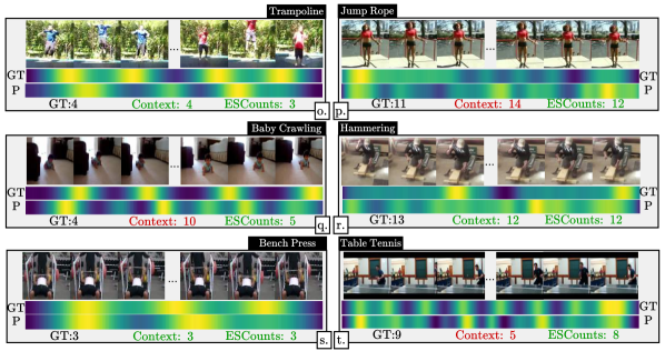
VRC metrics only relate predicted to correct counts, regardless of whether the repetitions have been correctly identified. We thus investigate whether the peaks of the predicted density map align with the annotated start-end times of repetitions in the ground truth. Following action localisation methods [8, 18, 22], we adopt and adjust the Jaccard index for repetition localisation. Using the predicted density map we define different thresholds for salient regions of repetitions. As the values of peaks vary across videos, we apply thresholds relative to the maximum and minimum values, . We find all local maxima in and only keep those above threshold . We consider a repetition to be correctly located (TP) if at least one peak occurs within the start-end time of that repetition. Peaks that occur within the same repetition are counted as one. In contrast, peaks that do not overlap with repetitions are false positives (FP) and repetitions that do not overlap with any peak are false negatives (FN). We then calculate the Jaccard index as TP divided by all the correspondences (TP + FP + FN) as customary.

In Table 10 we report the Jaccard index over different thresholds alongside the Mean Average Precision (mAP) on RepCount. We select TransRAC [20] as a baseline due to their publicly available checkpoint. Across thresholds, ESCounts outperforms [20] with the most notable improvements observed over higher threshold values demonstrating that ESCounts predict density maps with higher contrast between higher and lower salient regions. For 0.9, 0.8, and 0.7 thresholds ESCounts demonstrates an +8.68%, +10.30%, and +8.10% improvement over [20].
9 Comparison with TransRAC over Groups
As in Sec. 4.3, we divide the videos into groups based on their counts, average repetition duration, and lengths. We compare ESCounts’ performance against TransRAC in each of these groups. As evident from Fig. 10, ESCounts performs significantly better than TransRAC on high counts. From Fig. 10, ESCounts performs strongly over varying repetition duration, whilst TransRAC struggles on videos with XS and XL repetitions. Fig. 10 shows that even though both TransRAC and ESCounts performance drops on longer videos, ESCounts perform significantly better on them.